Neutrino effective potential and damping in a fermion and scalar background in the resonance region

Abstract

We consider the propagation of a neutrino or an antineutrino in a medium composed of fermions ($f$) and scalars ($\phi$) interacting via a Yukawa-type coupling of the form $\bar{f}\nu\phi$, for neutrino energies at which the processes like $\nu+\phi\leftrightarrow f$ or $\nu+\bar{f}\leftrightarrow\bar{\phi}$, and the corresponding ones for the antineutrino, are kinematically accessible. The relevant energy values are around $|m^{2}_{\phi}-m^{2}_{f}|/2m_{\phi}$ or $|m^{2}_{\phi}-m^{2}_{f}|/2m_{f}$, where $m_{\phi}$ and $m_{f}$ are the masses of $\phi$ and $f$, respectively. We refer to either one of these regions as a resonance energy range. Near these points, the one-loop formula for the neutrino self-energy has a singularity. From a technical point of view, that feature is indicative that the self-energy acquires an imaginary part, which is associated with damping effects and cannot be neglected, while the integral formula for the real part must be evaluated using the principal value of the integral. We carry out the calculations explicitly for some cases that allow us to give analytic results. Writing the dispersion relation in the form $\omega=\kappa+V_{\text{eff}}-i\gamma/2$, we give the explicit formulas for $V_{\text{eff}}$ and $\gamma$ for the cases considered. When the neutrino energy is either much larger or much smaller than the resonance energy, $V_{\text{eff}}$ reduces to the effective potential that has been already determined in the literature in the high or low momentum regime, respectively. The virtue of the formula we give for $V_{\text{eff}}$ is that it is valid also in the resonance energy range, which is outside the two limits mentioned. As a guide to possible applications we give the relevant formulas for $V_{\text{eff}}$ and $\gamma$, and consider the solution to the oscillation equations including the damping term, in a simple two-generation case.

1 Introduction and Summary

As is well known, the properties of neutrinos that propagate through a medium differ from those in the vacuum. In particular, the energy-momentum for massless neutrinos $\omega=\kappa$, where $\omega$ is the energy and $\kappa$ the magnitude of the momentum vector, is not valid in the medium[1, 2]. The modifications of the neutrino dispersion relation can be represented in terms of an index of refraction, or more suitable for our purposes, in terms of an effective potential ($V_{\text{eff}}$) and a damping ($\gamma$), by writing it in the generic form

$$\omega=\kappa+V_{\text{eff}}-i\gamma/2\,.$$ (1.1)

It is now well established that an efficient method to determine the dispersion relation, is to compute $V_{\text{eff}}$ and $\gamma$ from the calculation of the neutrino thermal self-energy[3, 4, 5, 6] in the framework of thermal field theory[7].

In several models and extensions of the standard electro-weak theory the neutrinos interact with scalar particles ($\phi$) and fermions ($f$) via a coupling of the form $\bar{f}_{R}\nu_{L}\phi$ or just with neutrinos $\bar{\nu}^{c}_{R}\nu_{L}\phi$. Couplings of the latter form have been explored recently in various contexts[8, 9, 10, 11, 12, 13, 14, 15, 16]. Such couplings produce additional contributions beyond the standard ones to the neutrino effective potential when the neutrino propagates in a neutrino background, as it occurs in the environment of a supernova, where the effect leads to the collective neutrino oscillations and related phenomena(see for example Refs. [17] and [18] and the works cited therein), or in the hot plasma of the Early-Universe before the neutrinos decouple[19, 20]. Couplings of the form $\bar{f}_{R}\nu_{L}\phi$ produce additional contributions to the neutrino effective potential when the neutrino propagates in a background of $\phi$ and $f$ particles and their possible effects have been considered in the context of Dark Matter-neutrino interactions[21, 22, 23, 24, 25, 26, 27, 28, 29]. More recently it has been pointed out that observable effects of such scalar interactions, although precluded in terrestrial experiments, are still possible in future solar and supernovae neutrino data, and in cosmological observations such as cosmic microwave background and big bang nucleosynthesis data[30].

Motivated by these developments, we carried out in previous work a systematic calculation of the neutrino effective potential in such models[31]. We considered various cases, depending on the magnitude of $\kappa$ relative to other parameters such as the masses of the particles and the temperature of the background. In the limit of small $\kappa$, the effective potential becomes independent of $\kappa$ and has a form that is reminiscent of the Wolfenstein potential[1]. In the opposite limit (relatively large $\kappa$), the effective potential has a term proportional to $1/\kappa$ that mimics a contribution to the neutrino mass[32].

The main point that is relevant to the present work, is that in the intermediate $\kappa$ region, to be defined precisely below, neither limiting case is a valid approximation to the effective potential. From a physical point of view, there is a region of neutrino energies at which the processes like $\nu+\phi\leftrightarrow f$ or $\nu+\bar{f}\leftrightarrow\bar{\phi}$, and the corresponding ones for the antineutrino, become kinematically accessible. The relevant energy values are around $|m^{2}_{\phi}-m^{2}_{f}|/2m_{\phi}$ or $|m^{2}_{\phi}-m^{2}_{f}|/2m_{f}$, to which we refer as a resonance energy range. In those ranges, the one-loop integral formula for the neutrino self-energy has a singularity, as has been emphasized recently in Ref. [33].

From a technical point of view, the singularity is indicative of two things. Firstly, at those points the self-energy acquires an imaginary part that cannot be neglected. The imaginary part of the self-energy is associated with damping effects, and determines the damping term $\gamma$ in the dispersion relation. A systematic calculation of the damping terms was carried out in Ref. [34].

Secondly, and what is our main observation here, the effective potential, which is determined from the real (dispersive) part of the self-energy, must be evaluated using the principal value of the integral formula for the self-energy. The principal value prescription allows us to give a well-defined meaning to (the real part of) the integral for values of $\kappa$ around the singularities. Our purpose in this work is to carry out the calculation of the effective potential in the resonance regions using the strategy just explained. Writing the dispersion relation in the form given in Eq. (1.1), we give the explicit formulas for $V_{\text{eff}}$ and $\gamma$ for some cases that allow us to give analytic results, and indications for carrying out extensions and generalizations to other cases of interest. When the neutrino energy is either much larger or much smaller than the resonance energy, $V_{\text{eff}}$ reduces to the effective potential that has been already determined in the literature in the high or low momentum regime, respectively. The virtue of the formula we give for $V_{\text{eff}}$ is that it is valid also in the resonance energy range, which is outside the two limits mentioned. As a guide to possible applications to neutrino oscillations in the case that the neutrino energy is in the resonance region, we give the relevant formulas for the $V_{\text{eff}}$ and $\gamma$ terms that enter in the oscillation equations in a simple two-generation case, and consider their solution including the damping term.

In Section 2 we summarize our notation and conventions, and the context in which we carry out the calculations. In Section 3 we calculate the effective potential, paying special attention to the contribution from the resonance terms, which are expressed as an integral over the background particle momentum distribution functions. We consider in detail the evaluation of the relevant integral for the case that the resonance term is the fermion background contribution, and for concreteness we give the explicit formulas for the case of a non-relativistic and degenerate Fermi gas. Such formulas can be particularly useful for considering the implications and/or setting limits on the neutrino interactions with light particle dark matter backgrounds from their effect on the phenomenology in reactor, solar, atmospheric, and accelerator experiments. In Section 4 we consider the damping term. We discuss some generalizations and possible extensions of the results in Section 5.1, and the two-generation example case mentioned above in Section 5.2.

2 Preliminaries

In this section we review the context of the present work and state the problem on which we focus.

2.1 Context

For definiteness we consider only one neutrino flavor coupling to the fermion and scalar, which we denote simply by $\nu$, and write

$$L^{(f\nu\phi)}=\lambda\bar{f}_{R}\nu_{L}\phi+h.c\,.$$ (2.1)

We denote by $k^{\mu}$ the momentum four-vector of the propagating neutrino and by $u^{\mu}$ the velocity four-vector of the background medium. In the background medium’s own rest frame, $u^{\mu}$ takes the form

$$u^{\mu}=(1,\vec{0})\,,$$ (2.2)

and in this frame we write

$$k^{\mu}=(\omega,\vec{\kappa})\,.$$ (2.3)

Since we are considering only one background medium, we can take it to be at rest and therefore we adopt Eqs. (2.2) and (2.3) throughout. For completeness, we briefly review and borrow from Refs. [31] and [34] the formulas that we will use to determine the dispersion relations from the self-energy calculation. We remind that the calculations are based on the application of the real-time Thermal Field Theory methods.

The neutrino dispersion relation is determined by the solution of the equation

$$(k\hbox to0.0pt{\hss/}-\Sigma_{\text{eff}})\psi_{L}(k)=0\,,$$ (2.4)

where $\Sigma_{\text{eff}}$ is the neutrino thermal self-energy. $\Sigma_{\text{eff}}$ can be decomposed into its dispersive ($\Sigma_{r}$) and absorptive ($\Sigma_{i}$) parts,

$$\Sigma_{\text{eff}}=\Sigma_{r}+i\Sigma_{i}\,.$$ (2.5)

$\Sigma_{r}$ is given by the real (dispersive) part of the 11 element of the neutrino thermal self-energy matrix, while $\Sigma_{i}$ is determined from the 12 element.

The chirality of the neutrino interactions implies that $\Sigma_{\text{eff}}$ has the form

$$\Sigma_{\text{eff}}=V\hbox to0.0pt{\hss/}L\,,$$ (2.6)

where $L=\frac{1}{2}(1-\gamma_{5})$. Corresponding to the decomposition of $\Sigma_{\text{eff}}$ in Eq. (2.5),

$$V^{\mu}=V^{\mu}_{r}+iV^{\mu}_{i}\,,$$ (2.7)

where $V^{\mu}_{r}$ and $V^{\mu}_{i}$ are real. $V_{r}$ and $V_{i}$ are functions of $\omega$ and $\vec{\kappa}$, but to simplify the notation we omit writing the arguments unless it is necessary to indicate them.

Equation (2.4) has two solutions. Denoting them by $\omega^{(\lambda)}$ ($\lambda=\pm$), they are determined by the equation

$$\omega^{(\lambda)}=V^{0}(\omega^{(\lambda)},\vec{\kappa})+\lambda[(\vec{\kappa}-\vec{V}(\omega^{(\lambda)},\vec{\kappa}))\cdot(\vec{\kappa}-\vec{V}(\omega^{(\lambda)},\vec{\kappa}))]^{1/2}\,,$$ (2.8)

or to lowest order,

$$\omega^{(\lambda)}=V^{0}(\omega^{(\lambda)},\vec{\kappa})+\lambda(\kappa-\hat{\kappa}\cdot\vec{V}(\omega^{(\lambda)},\vec{\kappa}))\,.$$ (2.9)

The neutrino ($\omega^{(\nu)}$) and antineutrino ($\omega^{(\bar{\nu})}$)dispersion relations are identified as

$$\omega^{(\nu)}(\vec{\kappa}) = \omega^{(+)}(\vec{\kappa})\,,$$

$$\omega^{(\bar{\nu})}(\vec{\kappa}) = \left(-\omega^{(-)}(-\vec{\kappa})\right)^{\ast}\,.$$ (2.10)

Decomposing $\omega^{(\nu)}$ and $\omega^{(\bar{\nu})}$ in terms of their real and imaginary parts in the form ($x=\nu,\bar{\nu}$),

$$\omega^{(x)}=\omega^{(x)}_{r}-\frac{i}{2}\gamma^{(x)}\,,$$ (2.11)

and assuming that it is a valid approximation to set

$$\gamma^{(x)}_{i} \ll |\omega^{(x)}_{r}|\,,$$

$$\omega^{(x)}_{r} \simeq \kappa\,,$$ (2.12)

Eq. (2.9) gives, for the real part

$$\omega^{(\nu)}_{r} = \kappa+V^{(\nu)}_{\text{eff}}(\vec{\kappa})\,,$$

$$\omega^{(\bar{\nu})}_{r} = \kappa+V^{(\bar{\nu})}_{\text{eff}}(\vec{\kappa})\,,$$ (2.13)

while for the imaginary part

$$-\frac{1}{2}\gamma^{(\nu)} = \frac{n\cdot V_{i}(\kappa,\vec{\kappa})}{1-n\cdot\left.\frac{\partial V_{r}(\omega,\vec{\kappa})}{\partial\omega}\right|_{\omega=\kappa}}\,,$$

$$-\frac{1}{2}\gamma^{(\bar{\nu})} = \frac{n\cdot V_{i}(-\kappa,-\vec{\kappa})}{1-n\cdot\left.\frac{\partial V_{r}(\omega,-\vec{\kappa})}{\partial\omega}\right|_{\omega=-\kappa}}\,,$$ (2.14)

where

$$V^{(\nu)}_{\text{eff}}(\vec{\kappa}) = n\cdot V_{r}(\kappa,\vec{\kappa})\,,$$

$$V^{(\bar{\nu})}_{\text{eff}}(\vec{\kappa}) = -n\cdot V_{r}(-\kappa,-\vec{\kappa})\,,$$ (2.15)

with

$$n^{\mu}=(1,\hat{\kappa})\,.$$ (2.16)

In those cases in which the correction due to the $n\cdot\partial V_{r}(\omega,\vec{\kappa})/\partial\omega$ in the denominator can be neglected, the formulas in Eq. (2.1) simplify to

$$-\frac{\gamma^{(\nu)}(\vec{\kappa})}{2} = n\cdot V_{i}(\kappa,\vec{\kappa})\,,$$

$$-\frac{\gamma^{(\bar{\nu})}(\vec{\kappa})}{2} = n\cdot V_{i}(-\kappa,-\vec{\kappa})\,,$$ (2.17)

which are the ones we will use here, borrowing from the work in Ref. [34].

2.2 Statement of the problem

To state the problem in concrete terms and set the stage for the work that follows, we recall (see, e.g, Ref. [31]) the following expression for the background-dependent part of the 11 element of the thermal self-energy matrix in the $f$ and $\phi$ background,

$$\Sigma_{11}(k)=\Sigma^{(f)}_{11}(k)+\Sigma^{(\phi)}_{11}(k)\,,$$ (2.18)

where

$$\Sigma^{(f)}_{11} = -|\lambda|^{2}\int\frac{d^{4}p}{(2\pi)^{3}}\frac{p\hbox to0.0pt{\hss/}L}{(p-k)^{2}-m^{2}_{\phi}+i\epsilon}\delta(p^{2}-m^{2}_{f})\eta_{f}(p)\,,$$ (2.19)

$$\Sigma^{(\phi)}_{11} = |\lambda|^{2}\int\frac{d^{4}p}{(2\pi)^{3}}\frac{(p\hbox to0.0pt{\hss/}+k\hbox to0.0pt{\hss/})L}{(p+k)^{2}-m^{2}_{f}+i\epsilon}\delta(p^{2}-m^{2}_{\phi})\eta_{\phi}(p)\,.$$ (2.20)

Using the label $x$ to stand for either $f$ or $\phi$, the functions $\eta_{x}(p)$ are given by

$$\eta_{x}(p)=\theta(p^{0})f_{x}(p^{0})+\theta(-p^{0})f_{\bar{x}}(-p^{0})\,,$$ (2.21)

where $f_{x,\bar{x}}(p^{0})$ are the equilibrium momentum distribution functions of the background particles and antiparticles,

$$f_{f,\bar{f}}(p^{0}) = \frac{1}{e^{\beta p^{0}\mp\alpha_{f}}+1}\,,$$

$$f_{\phi,\bar{\phi}}(p^{0}) = \frac{1}{e^{\beta p^{0}\mp\alpha_{\phi}}-1}\,,$$ (2.22)

where $\beta=1/T$ and $\alpha_{x}=\beta\mu_{x}$, with $T$ being the temperature and $\mu_{x}$ the chemical potentials.

To be precise, we mention that in Eq. (2.18) we are neglecting the term that involves the product of the two thermal parts of the propagators, which does not contribute to the real part of $\Sigma_{11}$. Thus, going back to Eq. (2.5), the dispersive part $\Sigma_{r}$ is given by

$$\Sigma_{r}=\Sigma^{(f)}_{r}+\Sigma^{(\phi)}_{r}\,,$$ (2.23)

where

$$\Sigma^{(f)}_{r} = -|\lambda|^{2}\int\frac{d^{4}p}{(2\pi)^{3}}\frac{p\hbox to0.0pt{\hss/}L}{(p-k)^{2}-m^{2}_{\phi}}\delta(p^{2}-m^{2}_{f})\eta_{f}(p)\,,$$ (2.24)

$$\Sigma^{(\phi)}_{r} = |\lambda|^{2}\int\frac{d^{4}p}{(2\pi)^{3}}\frac{(p\hbox to0.0pt{\hss/}+k\hbox to0.0pt{\hss/})L}{(p+k)^{2}-m^{2}_{f}}\delta(p^{2}-m^{2}_{\phi})\eta_{\phi}(p)\,.$$ (2.25)

In Eqs. (2.24) and (2.25), and the integrals that follow, the integrations are to be interpreted in the sense of their principal value.

Carrying out the integral over $p^{0}$, we obtain

$$n\cdot V_{r}(\omega,\vec{\kappa}) = v_{f}(\omega,\vec{\kappa})+v_{\bar{f}}(\omega,\vec{\kappa})+v_{\phi}(\omega,\vec{\kappa})+v_{\bar{\phi}}(\omega,\vec{\kappa})\,,$$ (2.26)

where

$$v_{f}(\omega,\vec{\kappa}) =-|\lambda|^{2}\int\frac{d^{3}p}{(2\pi)^{3}2E_{f}}(n\cdot p)\frac{f_{f}(\vec{p})}{D_{f}(k,p)}\,,$$ (2.27a)

$$v_{\bar{f}}(\omega,\vec{\kappa}) =|\lambda|^{2}\int\frac{d^{3}p}{(2\pi)^{3}2E_{f}}(n\cdot p)\frac{f_{\bar{f}}(\vec{p})}{D_{f}(k,-p)}\,,$$ (2.27b)

$$v_{\phi}(\omega,\vec{\kappa}) =|\lambda|^{2}\int\frac{d^{3}p}{(2\pi)^{3}2E_{\phi}}\frac{(n\cdot p+(\omega-\kappa))f_{\phi}(\vec{p})}{D_{\phi}(k,p)}\,,$$ (2.27c)

$$v_{\bar{\phi}}(\omega,\vec{\kappa}) =|\lambda|^{2}\int\frac{d^{3}p}{(2\pi)^{3}2E_{\phi}}\frac{(-n\cdot p+(\omega-\kappa))f_{\bar{\phi}}(\vec{p})}{D_{\phi}(k,-p)}\,,$$ (2.27d)

with

$$E_{x}=\sqrt{{\vec{p}\,}^{2}+m^{2}_{x}}\,,\qquad(x=f,\phi)\,,$$ (2.28)

$$D_{f}(k,p) = (p-k)^{2}-m^{2}_{\phi}=k^{2}-2p\cdot k+m^{2}_{f}-m^{2}_{\phi}\,,$$

$$D_{\phi}(k,p) = (p+k)^{2}-m^{2}_{f}=k^{2}+2p\cdot k+m^{2}_{\phi}-m^{2}_{f}\,,$$ (2.29)

and

$$n\cdot p=E_{x}(1-\hat{\kappa}\cdot\vec{v}_{x})\,.$$ (2.30)

In Eq. (2.30) $\vec{v}_{x}$ stands for the velocity of the background particle.

To bring out the issue that we want to address, consider for example the contribution from the $\bar{f}$ background, and suppose that the conditions are such that it can be treated in the non-relativistic limit. Then approximating

$$p^{\mu}\rightarrow(m_{f},\vec{0})\,,$$ (2.31)

in the integrand, $v_{\bar{f}}(\kappa,\vec{\kappa})$ is inversely proportional to

$$\left.D_{f}(k,-p)\right|_{\omega=\kappa}\simeq 2m_{f}\omega-(m^{2}_{\phi}-m^{2}_{f})\,.$$ (2.32)

Identifying the effective potential by Eq. (2.1), in the low momentum (heavy background) limit this gives a momentum-independent contribution to the effective potential reminiscent of the standard Wolfenstein term. In the opposite limit, the high momentum (or light background) limit this gives a term proportional to $1/\kappa$ that mimics a contribution to the neutrino mass[32]. But in the intermediate region the expression is not valid and actually undefined at

$$\omega\sim\frac{m^{2}_{\phi}-m^{2}_{f}}{2m_{f}}\,.$$ (2.33)

If $m_{\phi}>m_{f}$, physically this feature reflects the fact that in that regime the process $\nu+\bar{f}\rightarrow\bar{\phi}$ is kinematically accessible. In some cases the singularity appears for $\omega$ negative, which corresponds to the antineutrino dispersion relation. This is the case, in the example above, if $m_{f}>m_{\phi}$, and in that case the singularity corresponds to the process $\bar{f}\rightarrow\bar{\nu}+\bar{\phi}$. Similar considerations apply to the $v_{f}$ and the $\phi$ background terms. An exhaustive list of the various possibilities is summarized in Table 1.

	$v_{f}$	$v_{\bar{f}}$	$v_{\phi}$	$v_{\bar{\phi}}$
$m_{\phi}>m_{f}$	$-\Omega_{f}$	$\Omega_{f}$	$-\Omega_{\phi}$	$\Omega_{\phi}$
	$\bar{\nu}+f\rightarrow\phi$	$\nu+\bar{f}\rightarrow\bar{\phi}$	$\phi\rightarrow\bar{\nu}+f$	$\bar{\phi}\rightarrow\nu+\bar{f}$
$m_{f}>m_{\phi}$	$\Omega_{f}$	$-\Omega_{f}$	$\Omega_{\phi}$	$-\Omega_{\phi}$
	$f\rightarrow\nu+\phi$	$\bar{f}\rightarrow\bar{\nu}+\bar{\phi}$	$\nu+\phi\rightarrow f$	$\bar{\nu}+\bar{\phi}\rightarrow\bar{f}$

Table 1: List of possible resonance conditions in each background contribution and the associated physical processes. The parameters $\Omega_{x}$ are defined as $\Omega_{x}=|m^{2}_{\phi}-m^{2}_{f}|/2m_{x}$ (for $x=f,\phi)$, and they give the value of $\omega$ for which the indicated $v$ term, given in Eq. (2.27), is undefined, in the sense discussed in the text.

The bottom line is that near the resonance ranges indicated in the Table 1, the integrals in Eq. (2.27) must be handled following the principal value prescription, and approximations such as those we have indicated in Eqs. (2.31) and (2.32), which are commonly employed, are not valid in the cases we are considering.

Moreover, in those energy ranges, the corresponding damping term is not negligible. This can be seen from the calculation of the imaginary part of the self-energy, or equivalently $V^{\mu}_{i}$, in Ref. [34]. We will borrow the results of those calculations here without further ado. But regarding $V_{r}$, our proposal is to go back to Eq. (2.27) and evaluate those terms in a systematic way that is valid through the entire neutrino energy range.

3 Neutrino effective potential in the $\Omega_{f}$ region

For definiteness, we consider first the neutrino case in detail. To be clear and precise, in what follows we assume

$$m_{\phi}>m_{f}\,,$$ (3.1)

throughout. The opposite case can be treated in a similar way by making appropriate changes.

According to Table 1, the $v_{\bar{f}}$ and $v_{\bar{\phi}}$ terms have a resonance for $\omega=\Omega_{f}$ and $\omega=\Omega_{\phi}$, respectively, which we write in the form

$$\Omega_{f} = \frac{\Delta^{2}_{\phi f}}{2m_{f}}\,,$$

$$\Omega_{\phi} = \frac{\Delta^{2}_{\phi f}}{2m_{\phi}}\,,$$ (3.2)

where

$$\Delta^{2}_{\phi f}=m^{2}_{\phi}-m^{2}_{f}\,.$$ (3.3)

We assume that $m_{f}$ and $m_{\phi}$ are significantly different, such that $\Omega_{f,\phi}$ are sufficiently far apart and the two resonance regions do not overlap. For the purpose of evaluating the integrals this assumption is not strictly necessary, but the physical picture is conceptually clearer if we adopt it. Under this assumption we can consider each region separately. Thus we consider first the region

$$\omega\sim\kappa\sim\Omega_{f}\,,$$ (3.4)

which is the resonance region of $v_{\bar{f}}(\omega,\vec{\kappa})$.

From Eqs. (2.1) and (2.26) we then have

$$V^{(\nu)}_{\text{eff}}(\vec{\kappa})=U+r\,,$$ (3.5)

where

$$U\equiv v_{\bar{f}}(\kappa,\vec{\kappa})\,,$$ (3.6)

and

$$r=v_{f}(\kappa,\vec{\kappa})+v_{\phi}(\kappa,\vec{\kappa})+v_{\bar{\phi}}(\kappa,\vec{\kappa})\,.$$ (3.7)

As already mentioned, the evaluation of $r$ is straightforward. For example, let us consider the case that the $f$ background can be treated in the non-relativistic limit. In this case $v_{f}(\omega,\vec{\kappa})$ reduces to

$$v_{f}(\omega,\vec{\kappa})=\frac{\frac{1}{8}|\lambda|^{2}n_{f}}{m_{f}(\omega+\Omega_{f})}\,.$$ (3.8)

Since we are considering the case $m_{\phi}>m_{f}$, the $\phi$ and $\bar{\phi}$ backgrounds must be considered in the non-relativistic limit as well. Thus in this case,

$$v_{\phi}(\omega,\vec{\kappa}) =\frac{\frac{1}{4}|\lambda|^{2}n_{\phi}}{m_{\phi}(\omega+\Omega_{\phi})}\,,$$ (3.9a)

$$v_{\bar{\phi}}(\omega,\vec{\kappa}) =\frac{\frac{1}{4}|\lambda|^{2}n_{\bar{\phi}}}{m_{\phi}(\omega-\Omega_{\phi})}\,.$$ (3.9b)

Since we are considering $m_{\phi}>m_{f}$ and assuming that these masses are such that the resonance regions $\omega\sim\Omega_{f}$ and $\omega\sim\Omega_{\phi}$ are well separated, for the case of neutrino propagation near $\omega\sim\Omega_{f}$ we can put $\omega\gg\Omega_{\phi}$ in Eq. (3.9). Thus,

$$v_{\phi}(\omega,\vec{\kappa}) \simeq \frac{\frac{1}{4}|\lambda|^{2}n_{\phi}}{m_{\phi}\omega}\,,$$

$$v_{\bar{\phi}}(\omega,\vec{\kappa}) \simeq \frac{\frac{1}{4}|\lambda|^{2}n_{\bar{\phi}}}{m_{\phi}\omega}\,,$$ (3.10)

and therefore

$$r=|\lambda|^{2}\left[\frac{n_{f}}{8m_{f}(\kappa+\Omega_{f})}+\frac{(n_{\phi}+n_{\bar{\phi}})}{4m_{\phi}\kappa}\right]\,.$$ (3.11)

For later reference, it is useful to record that for $\omega$ and $\kappa$ away from the resonance region, $v_{\bar{f}}$ is given by a formula analogous to those quoted above for the other potential terms,

$$v_{\bar{f}}(\omega,\vec{\kappa})=\frac{\frac{1}{8}|\lambda|^{2}n_{\bar{f}}}{m_{f}(\omega-\Omega_{f})}=\frac{\frac{1}{8}|\lambda|^{2}n_{\bar{f}}}{m_{f}}\left\{\begin{array}[]{cc}\frac{1}{\omega}&(\omega\gg\Omega_{f})\\ -\frac{1}{\Omega_{f}}&(\omega\ll\Omega_{f})\,.\end{array}\right.$$ (3.12)

Regarding the damping terms defined in Eqs. (2.11) and (2.1) we can borrow literally the results given in Ref. [34].

3.1 Solution

Away from the kinematic points where $D_{f}(k,-p)$ does not vanish, the procedure of taking the principal value is not necessary. But if the kinematics is such that the integration covers the point at which $D_{f}(k,-p)=0$, the principal value operation defines the integral around that point.

We assume the $\bar{f}$ gas can be treated in the non-relativistic (NR) limit. Therefore we take

$$p^{\mu}=(m_{f},\vec{p})\,.$$ (3.13)

Then doing the angular integral, remembering the principal value prescription, we get

$$v_{\bar{f}}(\omega,\vec{\kappa})=\frac{|\lambda|^{2}}{8\pi^{2}}\int dp\;p^{2}\frac{f_{\bar{f}}(p)}{2p\kappa}\log\left|\frac{k^{2}+2m_{f}\omega+2p\kappa-\Delta^{2}_{\phi f}}{k^{2}+2m_{f}\omega-2p\kappa-\Delta^{2}_{\phi f}}\right|\,,$$ (3.14)

Further, we put

$$k^{2}=(\omega+\kappa)(\omega-\kappa)\rightarrow 2\kappa(\omega-\kappa)\,,$$ (3.15)

so that

$$k^{2}+2m_{f}\omega\pm 2p\kappa-\Delta^{2}_{\phi f}=2\kappa\left[\left(1+\frac{m_{f}}{\kappa}\right)(\omega-\kappa)\pm p+\frac{m_{f}}{\kappa}(\kappa-\Omega_{f})\right]\,,$$ (3.16)

and therefore

$$v_{\bar{f}}(\omega,\vec{\kappa})=\frac{|\lambda|^{2}}{16\pi^{2}\kappa}\int dp\;pf_{\bar{f}}(p)\log\left|\frac{\omega-\kappa+b+ap}{\omega-\kappa+b-ap}\right|\,,$$ (3.17)

with

$$a = \frac{1}{1+\frac{m_{f}}{\kappa}}\,,$$

$$b = \frac{\kappa-\Omega_{f}}{1+\frac{\kappa}{m_{f}}}\,.$$ (3.18)

Our next job is to evaluate the integral

$$I(\omega,\kappa)=\int dp\;pf_{\bar{f}}(p)\log\left|\frac{\omega-\kappa+b+ap}{\omega-\kappa+b-ap}\right|\,,$$ (3.19)

which is of the form encountered in the original calculation by Weldon[3] and similar calculations of the fermion self-energy in various physical contexts[35].

3.2 Evaluation of $v_{\bar{f}}$ for a Fermi gas

For definiteness, we consider the case in which the $\bar{f}$ background can be treated in the completely degenerate limit. We then write

$$v_{\bar{f}}(\omega,\vec{\kappa})=\frac{|\lambda|^{2}}{16\pi^{2}\kappa}I_{F}(\omega,\kappa)\,,$$ (3.20)

where

$$I_{F}(\omega,\kappa)=\int^{p_{F}}_{0}dp\;p\log\left|\frac{p+A}{p-A}\right|\,,$$ (3.21)

with

$$A=\frac{\omega-\kappa+b}{a}=\omega-\kappa+\frac{m_{f}}{\kappa}(\omega-\Omega_{f})\,.$$ (3.22)

A straightforward evaluation of the integral in Eq. (3.21) leads to

$$I_{F}(\omega,\kappa)=\frac{1}{2}(p^{2}_{F}-A^{2})\log\left|\frac{p_{F}+A}{p_{F}-A}\right|+Ap_{F}\,.$$ (3.23)

We can now use this to find the expression for the effective potential (in a NR Fermi gas) which, we repeat, is valid for the entire range of the neutrino momentum. $v_{\bar{f}}(\omega,\vec{\kappa})$ is given by Eq. (3.20), with $A$ defined in Eq. (3.22).

3.3 Formula for $v_{\bar{f}}(\kappa,\vec{\kappa})$

First of all, as a check, let us consider the limit of small $p_{F}$. Expanding the $\log$ function up to terms of order $p^{3}_{F}$, it follows that

$$I_{F}=\frac{2p^{3}_{F}}{3A}\,.$$ (3.24)

From Eq. (3.20), this gives

$$v_{\bar{f}}(\omega,\vec{\kappa})\simeq\frac{\frac{1}{8}|\lambda|^{2}n_{\bar{f}}}{m_{f}(\omega-\Omega_{f})}\,,$$ (3.25)

where we have used $p^{3}_{F}=3\pi^{2}n_{\bar{f}}$, and from Eq. (3.22), $A\sim\frac{m_{f}}{\kappa}(\omega-\Omega_{f})$ for $\omega\sim\kappa$. It is reassuring to see that the formula for $v_{\bar{f}}(\omega,\vec{\kappa})$ in Eq. (3.25) coincides with Eq. (3.12), which is obtained by taking $p^{\mu}\rightarrow(m_{f},\vec{0})$ from the beginning in the integrand. However, as we have emphasized, this limiting form is not valid for values of $\kappa$ near the resonance point.

In the general case, going back to Eq. (3.23),

$$\frac{I_{F}(\kappa,\kappa)}{p^{2}_{F}}=\frac{1}{2}(1-\eta^{2})\log\left|\frac{1+\eta}{1-\eta}\right|+\eta\,,$$ (3.26)

where

$$\eta=\frac{m_{f}}{p_{F}}\frac{\xi-1}{\xi}\,,$$ (3.27)

with

$$\xi=\frac{\kappa}{\Omega_{f}}\,.$$ (3.28)

Using Eq. (3.26) in Eq. (3.20),

$$U(\kappa)=v_{\bar{f}}(\kappa,\vec{\kappa})=U_{0}\frac{1}{\xi}\left[\frac{1}{2}(1-\eta^{2})\log\left|\frac{1+\eta}{1-\eta}\right|+\eta\right]\,,$$ (3.29)

where

$$U_{0}=\frac{|\lambda|^{2}p^{2}_{F}}{16\pi^{2}\Omega_{f}}\,.$$ (3.30)

The formula in Eq. (3.29) is our main result. For reference, a plot of $U(\kappa)$ is shown in Fig. 1.

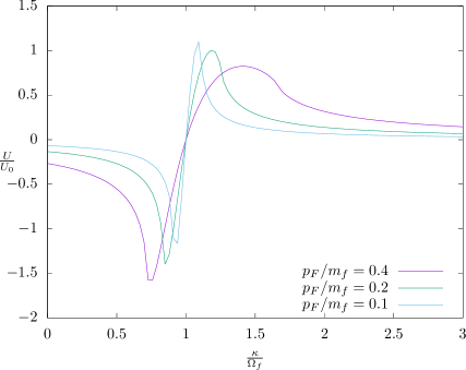
Figure 1: Plot of $U(\kappa)$, for $\kappa\sim\Omega_{f}$, with some example values of $p_{F}/m_{f}$.

We note the following. Away from the resonance region, $\eta$ has the limiting values

$$\eta=\frac{m_{f}}{p_{F}}\left\{\begin{array}[]{ll}-\frac{1}{\xi}&\mbox{(low $\kappa$)}\\ 1&\mbox{(high $\kappa$)}\,.\end{array}\right.$$ (3.31)

Therefore, either in the high ($\kappa\gg\Omega_{f}$) or low ($\kappa\ll\Omega_{f}$) momentum limit, $\eta$ is large and we can approximate $I_{F}(\kappa,\vec{\kappa})$ by its limiting value for large $\eta$, which gives

$$\frac{I_{F}(\kappa,\vec{\kappa})}{p^{2}_{F}}\simeq\frac{2}{3\eta}=\frac{2p_{F}}{3m_{f}}\left(\frac{\xi}{\xi-1}\right)\,.$$ (3.32)

Then from Eq. (3.20), this reproduces, again, Eq. (3.25). Thus, in these asymptotic limits, namely high or low momentum as specified above, the expression for $v_{\bar{f}}(\kappa,\vec{\kappa})$ given in Eq. (3.29) coincides with the results that are obtained by approximating from the beginning the integrals for $v_{\bar{f}}$ under the same conditions, namely, away from the resonance and for the non-relativistic limit. However, as we can see from Eq. (3.27), $|\eta|<1$ for values of $\kappa$ such that $|\xi-1|<p_{F}/m_{f}$, so that in this range the asymptotic form of $I_{F}$ given in Eq. (3.32) is not valid.

The virtue of Eq. (3.29) is that it is valid also in the resonance region, interpolating between the asymptotic expressions corresponding to high or low $\kappa$ mentioned above, and they allow us to consider the propagation in the resonance region, including the range $|\kappa/\Omega_{f}-1|<p_{F}/m_{f}$ mentioned. On the other hand, the imaginary part of the dispersion relation is important in that region, as we have remarked, and it must be included in the treatment of the propagation equation. As a guide to possible applications we consider that next.

4 Damping term

The damping term $\gamma^{(\nu)}$ in Eq. (2.11) is not negligible in the resonance region. As indicated in Eq. (2.1), it is determined from the absorptive part $V^{\mu}_{i}$ of the effective potential which in turn is determined from the $\Sigma_{12}$ element of the thermal self-energy matrix. That calculation was carried out in detail in Ref. [34]. As shown in that reference, the resulting formula for $\gamma^{(\nu)}$ is related to the transition probabilities for the various processes in which the neutrino may be annihilated or created, such as $\nu+\bar{f}\leftrightarrow\bar{\phi}$ and $\nu+\phi\leftrightarrow f$, in the forward and reverse directions. The formulas involve the phase space integrals weighted by the appropriate momentum distribution functions. Here we just need to borrow the results of those calculations. Quoting the results that are summarized in Eq. (3.38) of Ref. [34],

$$\frac{\gamma^{(\nu)}(\kappa)}{2}=\frac{|\lambda|^{2}}{32\pi\kappa^{2}\beta}\left\{\begin{array}[]{ll}\Delta^{2}_{f\phi}\left[\log\left(1+e^{-\beta E^{(I)}_{min}+\alpha_{f}}\right)-\log\left(1-e^{-\beta\Omega^{(I)}_{min}+\alpha_{\phi}}\right)\right]&(m_{f}>m_{\phi})\\[12.0pt] \Delta^{2}_{\phi f}\left[\log\left(1+e^{-\beta E^{(II)}_{min}-\alpha_{f}}\right)-\log\left(1-e^{-\beta\Omega^{(II)}_{min}-\alpha_{\phi}}\right)\right]&(m_{\phi}>m_{f})\,.\end{array}\right.$$ (4.1)

The corresponding formulas for $\frac{\gamma^{(\bar{\nu})}(\kappa)}{2}$ are obtained by making the substitutions

$$\alpha_{f,\phi}\rightarrow-\alpha_{f,\phi}\,.$$ (4.2)

To be consistent with Eq. (3.1), we focus on the second formula in Eq. (4.1). In that formula,

$$\Omega^{(II)}_{min} = \frac{\Delta^{2}_{\phi f}}{4\kappa}+\frac{\kappa m^{2}_{\phi}}{\Delta^{2}_{\phi f}}\,,$$

$$E^{(II)}_{min} = \frac{\Delta^{2}_{\phi f}}{4\kappa}+\frac{\kappa m^{2}_{f}}{\Delta^{2}_{\phi f}}\,,$$ (4.3)

with $\Delta^{2}_{\phi f}$ defined in Eq. (3.3). The term involving $\alpha_{f}$ corresponds to the contribution from the $\bar{f}$ gas in the background, while the term with $\alpha_{\phi}$ corresponds to the $\bar{\phi}$ gas, which are associated with the processes $\nu+\bar{f}\leftrightarrow\bar{\phi}$ and $\nu+\phi\leftrightarrow f$, respectively.

To complement our calculation of the effective potential in the previous section, here we want to calculate the $\bar{f}$ background contribution to the damping in the case that it can be considered as a completely degenerate fermion gas. In order to bring out the physical picture in a clearer way, let us consider first the case that both the $\bar{\phi}$ and $\bar{f}$ gases can be treated in the classical and non-relativistic limit.

4.1 Damping in the classical and non-relativistic (NR) limit

In that case

$$\frac{\gamma^{(\nu)}(\kappa)}{2} = \frac{|\lambda|^{2}}{32\pi\kappa^{2}\beta}\Delta^{2}_{\phi f}\left[e^{-\beta E^{(II)}_{min}-\alpha_{f}}+e^{-\beta\Omega^{(II)}_{min}-\alpha_{\phi}}\right]\,,$$ (4.4)

where in the non-relativistic limit (as we have assumed in Section 3.1), the chemical potentials are

$$e^{-\alpha_{f}} = \frac{1}{2}n_{\bar{f}}\left(\frac{2\pi\beta}{m_{f}}\right)^{\frac{3}{2}}e^{\beta m_{f}}\,,$$

$$e^{-\alpha_{\phi}} = n_{\bar{\phi}}\left(\frac{2\pi\beta}{m_{\phi}}\right)^{\frac{3}{2}}e^{\beta m_{\phi}}\,.$$ (4.5)

Therefore,

$$\frac{\gamma^{(\nu)}(\kappa)}{2}=\frac{\Omega^{2}_{f}}{\kappa^{2}}\frac{\gamma^{(0)}_{\bar{f}}}{2}e^{-\Lambda_{f}}+\frac{\Omega^{2}_{\phi}}{\kappa^{2}}\frac{\gamma^{(0)}_{\bar{\phi}}}{2}e^{-\Lambda_{\phi}}\,,$$ (4.6)

where

$$\frac{\gamma^{(0)}_{\bar{f}}}{2} = \frac{|\lambda|^{2}}{16}\sqrt{\frac{2\pi T}{m_{f}}}\frac{n_{\bar{f}}}{T\Omega_{f}}\,,$$

$$\frac{\gamma^{(0)}_{\bar{\phi}}}{2} = \frac{|\lambda|^{2}}{8}\sqrt{\frac{2\pi T}{m_{\phi}}}\frac{n_{\bar{\phi}}}{T\Omega_{\phi}}\,,$$

$$\Lambda_{f} = \frac{m_{f}}{2T}\frac{\left(\frac{\kappa}{\Omega_{f}}-1\right)^{2}}{\left(\frac{\kappa}{\Omega_{f}}\right)}\,,$$

$$\Lambda_{\phi} = \frac{m_{\phi}}{2T}\frac{\left(\frac{\kappa}{\Omega_{\phi}}-1\right)^{2}}{\left(\frac{\kappa}{\Omega_{\phi}}\right)}\,.$$ (4.7)

with $\Omega_{f,\phi}$ defined in Eq. (3).

The picture that emerges is consistent with our previous discussions regarding the resonances and complements it in a practical way. Outside of either resonance range the damping is exponentially small and can be neglected in the formula for the dispersion relation. Therefore, if we are considering a neutrino propagating in the $\Omega_{f}$ resonance region, we can discard the $\bar{\phi}$ contribution to the damping term, assuming, as we do, that $m_{f}$ and $m_{\phi}$ are sufficiently different that the resonances at $\Omega_{f}$ and $\Omega_{\phi}$ do not overlap.

For illustrative purposes we show a plot of $\gamma^{(\nu)}(\kappa)$ in Fig. 2 in the $\kappa\sim\Omega_{f}$ resonance region, obtained as follows. As already stated, we assume that $m_{f}$ and $m_{\phi}$ are sufficiently different that the resonances at $\Omega_{f}$ and $\Omega_{\phi}$ do not overlap; e.g., the $\kappa=\Omega_{\phi}$ point falls outside the range shown in the plot. Under this condition, in the $\Omega_{f}$ resonance region we can neglect the $\bar{\phi}$ contribution in Eq. (4.6) and consider simply

$$\frac{\gamma^{(\nu)}}{\gamma^{(0)}_{\bar{f}}}=\frac{1}{\xi^{2}}e^{-\frac{m_{f}}{2T}\frac{(\xi-1)^{2}}{\xi}}\,,$$ (4.8)

with $\xi$ defined in Eq. (3.28). Equation (4.8) is plotted in Fig. 2.

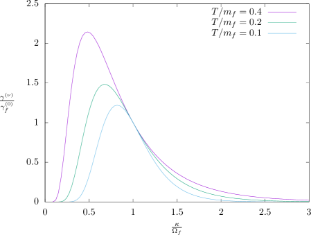
Figure 2: Plot of the damping term for $\kappa\sim\Omega_{f}$, given by Eq. (4.8), for some example values of $T/m_{f}$.

4.2 Damping in the degenerate limit

Armed with the results of the previous section, we thus ignore the $\bar{\phi}$ contribution to the damping, and as a complement to the formula for the effective potential in Eq. (3.29) here we calculate the $\bar{f}$ background contribution to $\gamma^{(\nu)}$, that is

$$\frac{\gamma^{(\nu)}(\kappa)}{2}=\frac{|\lambda|^{2}\Delta^{2}_{\phi f}}{32\pi\kappa^{2}\beta}\log\left(1+e^{-\beta E^{(II)}_{min}-\alpha_{f}}\right)\,,$$ (4.9)

in the limit of a completely degenerate fermion gas. This formula, and the results discussed below, hold in all the kinematic regime of the fermion gas, so they can be used in the NR case, or in any other case as well.

Setting

$$\alpha_{f}=-\beta E_{F}\,,$$ (4.10)

where $E_{F}$ is the Fermi energy, and taking the degenerate limit ($\beta\rightarrow\infty$),

$$\frac{\gamma^{(\nu)}(\kappa)}{2}=\frac{|\lambda|^{2}\Delta^{2}_{\phi f}}{32\pi\kappa^{2}}\left(E_{F}-E^{(II)}_{min}\right)\theta\left(E_{F}-E^{(II)}_{min}\right)\,.$$ (4.11)

The step function in Eq. (4.11) implies that $\gamma^{(\nu)}(\kappa)$ is non-zero if $\kappa$ lies in the range such that

$$\frac{1}{2}(E_{F}-p_{F})\leq\frac{\kappa m^{2}_{f}}{\Delta^{2}_{\phi f}}\leq\frac{1}{2}(E_{F}+p_{F})\,,$$ (4.12)

or it is zero otherwise. Equation (4.11) can be written in the form

$$\gamma^{(\nu)}=\gamma^{(0)}_{f}\frac{1}{\xi^{2}}\left[\frac{E_{F}}{m_{f}}-\frac{1}{2}\left(\xi+\frac{1}{\xi}\right)\right]\,,$$ (4.21)

for $\xi$, defined in Eq. (3.28), in the range

$$\frac{1}{m_{f}}(E_{f}-p_{F})\leq\xi\leq\frac{1}{m_{f}}(E_{F}+p_{F})\,,$$ (4.22)

and

$$\frac{\gamma^{(0)}_{f}}{2}=\frac{|\lambda|^{2}m^{2}_{f}}{16\pi\Omega_{f}}\,.$$ (4.23)

As already stated, the result given in Eq. (4.21) holds in all the kinematic regime of the fermion gas.

Eq. (4.21) is ploted in Fig. 3. The damping becomes smaller as $p_{F}$ decreases. From Fig. 1 we see that, at the same time, the width of the resonance peaks in the effective potential become narrower. These features indicate that the resonance effects are more important for relatively large values of $p_{F}$ (high density) and less important as $p_{F}$ decreases (lower density). A similar effect occurs with the damping in the classical case, which reduces as the temperature decreases, as shown in Fig. 2.

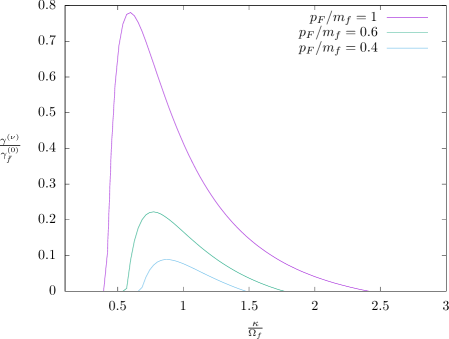
Figure 3: Plot of the damping term in the case of a degenerate $\bar{f}$ background, given by Eq. (4.21), for some example values of $p_{F}/m_{f}$.

5 Discussion

Here we discuss some generalizations and extensions of our work. On one hand, the case of antineutrinos, as well as the other resonance region, around $\omega\sim\Omega_{\phi}$ in the notation of Table 1, can be treated in analogous form. In order to point out possible differences in details and/or implementation we consider them briefly here.

On the other hand, since we have restricted ourselves to the case of one neutrino flavor propagating and interacting in the $f$ and $\phi$ background, as a guide and example to possible applications and generalizations, here we will consider the application to the oscillation equations including the damping term, in a simple two-generation case.

5.1 Anti-neutrino propagation near $\Omega_{f}$

Again we assume that $m_{\phi}>m_{f}$, and we consider the propagation at energies $\omega^{(\bar{\nu})}\sim\Omega_{f}$. This is the resonance region of the term $v_{f}$, which is the term that must be singled out for special consideration. From Eqs. (2.1) and (2.26) we have in the present case

$$V^{(\bar{\nu})}_{\text{eff}}(\vec{\kappa})=\bar{U}+\bar{r}\,,$$ (5.1)

where

$$\bar{U}=-v_{f}(-\kappa,-\vec{\kappa})\,,$$ (5.2)

and

$$\bar{r}=-v_{\bar{f}}(-\kappa,-\vec{\kappa})-v_{\phi}(-\kappa,-\vec{\kappa})-v_{\bar{\phi}}(-\kappa,-\vec{\kappa})\,.$$ (5.3)

For $v_{\phi}$ and $v_{\bar{\phi}}$, we can simply borrow the formulas given in Eqs. (3.9a) and (3), while for $v_{\bar{f}}(\omega,\vec{\kappa})$ the corresponding formula in this case is Eq. (3.12). Thus, mimicking the steps leading to Eq. (3.11), we obtain

$$\bar{r}=|\lambda|^{2}\left[\frac{n_{\bar{f}}}{8m_{f}(\kappa+\Omega_{f})}+\frac{(n_{\phi}+n_{\bar{\phi}})}{4m_{\phi}\kappa}\right]\,.$$ (5.4)

Regarding $v_{f}$, we go back to Eq. (2.27a). Carrying out the angular integral, remembering the principal value prescription,

$$v_{f}(\omega,\vec{\kappa})=-\frac{|\lambda|^{2}}{8\pi^{2}}\int dp\;p^{2}\frac{f_{f}(p)}{2p\kappa}\log\left|\frac{k^{2}-2m_{f}\omega+2p\kappa-\Delta^{2}_{\phi f}}{k^{2}-2m_{f}\omega-2p\kappa-\Delta^{2}_{\phi f}}\right|\,.$$ (5.5)

As we can see, $-v_{f}(-\omega,-\vec{\kappa})$ is given by the same expression given in Eq. (3.14) for $v_{\bar{f}}(\omega,\vec{\kappa})$, with the substitution $f_{\bar{f}}\rightarrow f_{f}$ in the integrand. Thus, for example, in the case that $f$ gas can be treated in the NR and degenerate limit, the net result of this is that the final formula for $\bar{U}$ is the same as the formula for $U$ given in Eq. (3.29), but of course with $p_{F}$ given in terms of the $f$ number density, $p^{3}_{F}=3\pi^{2}n_{f}$.

The damping can be treated similarly to the case of neutrinos in Section 4, but in the present case the relevant number densities are $n_{f}$ and $n_{\phi}$. Explicitly, remembering Eq. (4.2), in the classical and NR limit the damping is

$$\frac{\gamma^{(\bar{\nu})}(\kappa)}{2}=\frac{\Omega^{2}_{f}}{\kappa^{2}}\frac{\gamma^{(0)}_{f}}{2}e^{-\Lambda_{f}}+\frac{\Omega^{2}_{\phi}}{\kappa^{2}}\frac{\gamma^{(0)}_{\phi}}{2}e^{-\Lambda_{\phi}}\,,$$ (5.6)

where

$$\frac{\gamma^{(0)}_{f}}{2} = \frac{|\lambda|^{2}}{16}\sqrt{\frac{2\pi T}{m_{f}}}\frac{n_{f}}{T\Omega_{f}}\,,$$

$$\frac{\gamma^{(0)}_{\phi}}{2} = \frac{|\lambda|^{2}}{8}\sqrt{\frac{2\pi T}{m_{\phi}}}\frac{n_{\phi}}{T\Omega_{\phi}}\,,$$ (5.7)

with $\Lambda_{f,\phi}$ given by Eq. (4.1). For a degenerate $f$ gas, the formula for $\gamma^{(\bar{\nu})}$ is the same as Eq. (4.21), but with the reinterpretation of $p_{F}$ as the Fermi momentum associated with the $f$ gas number density $n_{f}$, as we have stated above. The sketches of the damping and the effective potential in this case are therefore similar to those shown in Figs. 1, 2 and 3 with the corresponding identification of the parameters involved.

In the case of a neutrino or antineutrino propagating near the $\Omega_{\phi}$ energy region, the same method can be applied to calculate the effective potential. In this case the term that must be singled out for special treatment is $v_{\bar{\phi}}$ (or $v_{\phi}$ for antineutrinos). The relevant integrals are of the same form given in Eq. (3.19), but they involve the $\bar{\phi}$ or $\phi$ distribution functions. In the classical limit of the distribution functions, the task involves the computation of the generic integrals

$$\int dx\,e^{-x^{n}}x\log\left|\frac{x+A}{x-A}\right|\,,$$ (5.8)

with $n=1,2$ in the ultra-relativistic and non-relativistic limits, respectively. Integrals of this form appear in similar calculations in other contexts as already mentioned[35]. We do not pursue this case any further here.

5.2 Two-generation example

We consider a two-generation case, assuming that only the first generation (e.g., electron neutrino) couples to $f$ and $\phi$. Working at the level of the evolution of the flavor spinor, the equation, including the damping term, is

$$i\partial_{t}\phi=\left(H_{r}-\frac{i}{2}\Gamma\right)\phi\,.$$ (5.9)

Up to a term proportional to identity matrix, the Hamiltonian is

$$H_{r}=\frac{1}{2}\frac{\Delta m^{2}_{21}}{2\kappa}\left(\begin{array}[]{cc}-\cos 2\theta&\sin 2\theta\\ \sin 2\theta&\cos 2\theta\end{array}\right)+\frac{1}{2}\left(\begin{array}[]{cc}V^{(\nu)}_{\text{eff}}&0\\ 0&-V^{(\nu)}_{\text{eff}}\end{array}\right)\,,$$ (5.10)

where $\Delta m^{2}_{21}=m^{2}_{2}-m^{2}_{1}$, while

$$\Gamma=\left(\begin{array}[]{cc}\gamma^{(\nu)}&0\\ 0&0\end{array}\right)\equiv\gamma^{(\nu)}I_{e}\,,$$ (5.11)

with

$$I_{e}\equiv\left(\begin{array}[]{cc}1&0\\ 0&0\end{array}\right)\,.$$ (5.12)

$V^{(\nu)}_{\text{eff}}$ and $\gamma^{(\nu)}$ are understood to be the effective potential and damping term that we have obtained.

Following the usual steps, $H_{r}$ can be written in the standard form

$$H_{r}=\frac{h}{2}\left(\begin{array}[]{cc}-\cos 2\theta_{m}&\sin 2\theta_{m}\\ \sin 2\theta_{m}&\cos 2\theta_{m}\end{array}\right)\,,$$ (5.13)

where

$$h=\frac{\Delta^{2}_{m}}{2\kappa}\,,$$ (5.14)

and

$$\cos 2\theta_{m} = \frac{1}{\Delta^{2}_{m}}\left(\Delta m^{2}_{21}\cos 2\theta-2\kappa V^{(\nu)}_{\text{eff}}\right)\,,$$

$$\sin 2\theta_{m} = \frac{\Delta m^{2}_{21}\sin 2\theta}{\Delta^{2}_{m}}\,,$$ (5.15)

with

$$\Delta^{2}_{m}\equiv\sqrt{(\Delta m^{2}_{21}\sin 2\theta)^{2}+\left(\Delta m^{2}_{21}\cos 2\theta-2\kappa V^{(\nu)}_{\text{eff}}\right)^{2}}\,.$$ (5.16)

Writing the solution in the form

$$\phi(t)=G\phi(0)\,,$$ (5.17)

in the absence of the damping term

$$G=\sum_{s=\pm}u_{s}u^{\dagger}_{s}e^{-i\lambda_{s}t}\,,$$ (5.18)

where $\lambda_{s}=sh$ are the eigenvalues of $H_{r}$, and $u_{s}$ the corresponding eigenspinors

$$u_{+} = \left(\begin{array}[]{c}\sin\theta_{m}\\ \cos\theta_{m}\end{array}\right)\,,$$ (5.21)

$$u_{-} = \left(\begin{array}[]{c}\cos\theta_{m}\\ -\sin\theta_{m}\end{array}\right)\,.$$ (5.24)

In the spirit of a perturbative treatment of the damping term, we construct the solution by taking the eigenvectors of $H$ to be the same as the eigenvectors of $H_{r}$, but with the eigenvalues modified by the first order corrections; i.e.,

$$\lambda_{s}=sh-\frac{i}{2}u^{\dagger}_{s}\Gamma u_{s}\,.$$ (5.25)

By explicitly calculation,

$$\lambda_{s}=\left\{\begin{array}[]{cc}h-\frac{i}{2}\gamma_{s}&(s=+)\\ -h-\frac{i}{2}\gamma_{c}&(s=-)\,,\end{array}\right.$$ (5.26)

where we have defined

$$\gamma_{s} = \gamma^{(\nu)}\sin^{2}\theta_{m}\,,$$

$$\gamma_{c} = \gamma^{(\nu)}\cos^{2}\theta_{m}\,.$$ (5.27)

We then obtain the following explicit expression for the evolution matrix

$$G=u_{+}u^{\dagger}_{+}e^{-iht}e^{-\frac{1}{2}\gamma_{s}t}+u_{-}u^{\dagger}_{-}e^{iht}e^{-\frac{1}{2}\gamma_{c}t}\,.$$ (5.28)

So, for example, for

$$\phi(0)=\left(\begin{array}[]{c}1\\ 0\end{array}\right)\,,$$ (5.29)

we have the persistence and transition amplitudes,

$$\phi_{1}(t) = \sin^{2}\theta_{m}e^{-iht}e^{-\frac{1}{2}\gamma_{s}t}+\cos^{2}\theta_{m}e^{iht}e^{-\frac{1}{2}\gamma_{c}t}\,,$$

$$\phi_{2}(t) = \sin\theta_{m}\cos\theta_{m}\left(e^{-iht}e^{-\frac{1}{2}\gamma_{s}t}-e^{iht}e^{-\frac{1}{2}\gamma_{c}t}\right)\,,$$ (5.30)

and the corresponding oscillation probabilities can be written in the form

$$P_{1}\equiv|\phi_{1}|^{2} = \frac{1}{2}\left(e^{-\gamma_{c}t}+e^{-\gamma_{s}t}\right)+\frac{1}{2}\cos 2\theta_{m}\left(e^{-\gamma_{c}t}-e^{-\gamma_{s}t}\right)$$

$$\mbox{}-\frac{1}{2}\sin^{2}2\theta_{m}\left[\frac{1}{2}\left(e^{-\gamma_{c}t}+e^{-\gamma_{s}t}\right)-e^{-\frac{1}{2}\gamma^{(\nu)}t}\cos 2ht\right]\,,$$

$$P_{2}\equiv|\phi_{2}|^{2} = \frac{1}{2}\sin^{2}2\theta_{m}\left[\frac{1}{2}\left(e^{-\gamma_{c}t}+e^{-\gamma_{s}t}\right)-e^{-\frac{1}{2}\gamma^{(\nu)}t}\cos 2ht\right]\,.$$ (5.31)

The importance of the damping terms depends on the interplay between $h$, defined in Eq. (5.14), and $\gamma^{(\nu)}$. To be more specific, we can consider, for example, the propagation of neutrinos near the $\Omega_{f}$ region, with $V^{(\nu)}_{\text{eff}}$ given by Eq. (3.5) (with $r$ and $U$ given by Eqs. (3.11) and (3.29), respectively) and $\gamma^{(\nu)}$ by Eq. (4.8). For small values of $\gamma^{(\nu)}$, many oscillation length cycles are required for the damping effects to be observable. A distinctive feature of Eq. (5.2) is the energy dependence of the damping and the oscillation terms, based on the formulas for $\gamma^{(\nu)}$ and $V^{(\nu)}_{\text{eff}}$ that we have given. For example, if we consider a pure $\bar{f}$ background (no $f$ and no $\phi,\bar{\phi}$ backgrounds) then $V^{(\nu)}_{\text{eff}}$ is given only by $U$ [Eqs. (3.5) and (3.29)], which becomes zero for neutrino energies very close to the resonance point $\Omega_{f}$. In that regime $h$ reduces to its vacuum value $\Delta m^{2}_{21}/2\kappa$ while the damping term reaches its largest value.

6 Conclusions and outlook

In this work we have been concerned with the propagation of a neutrino in a background of fermions ($f$) and scalars ($\phi$), interacting via a Yukawa-type interaction. Our particular goal was to obtain the dispersion relation in the case that the neutrino energy lies in the range in which the absorption and production processes become kinematically accessible, such as $\nu+\bar{f}\rightarrow\bar{\phi}$ or the crossed counterparts, and the corresponding ones for the antineutrino. The relevant energy values are around $|m^{2}_{\phi}-m^{2}_{f}|/2m_{f}$ or $|m^{2}_{\phi}-m^{2}_{f}|/2m_{\phi}$, to which we refer as a resonance energy range. The distinguishing aspect of these energy ranges is that the one-loop formula for the neutrino self-energy has a singularity, which is the indication that the self-energy acquires an imaginary part that cannot be ignored. Technically, the imaginary part is associated with the damping effects, while the integral formula for the real part must be evaluated using the principal value of the integral.

Writing the dispersion relation in the form $\omega=\kappa+V_{\text{eff}}-i\gamma/2$, we gave the explicit formulas for the effective potential ($V_{\text{eff}}$) and damping ($\gamma$) for some cases that allowed us to give analytic results. In particular we considered in detail the evaluation of those quantities for a neutrino propagating with the energy near ($m^{2}_{\phi}-m^{2}_{f})/2m_{f}$ (corresponding, for $m_{\phi}>m_{f}$, to the processes $\nu+\bar{f}\rightarrow\bar{\phi}$ becoming kinematically accessible), in the case that the $\bar{f}$ background can be treated as a non-relativistic degenerate Fermi gas. We also considered the analogous case for an antineutrino.

The formulas obtained have the property that, when the neutrino energy is either much larger or much smaller than the resonance energy, $V^{(\nu)}_{\text{eff}}$ reduces to the effective potential that has been already determined in the literature in the high or low momentum regime, respectively. The virtue of the formula we give for $V^{(\nu)}_{\text{eff}}$ is that it is valid also in the resonance energy range, which is outside the two limits mentioned. We outlined how the same strategy can be applied to consider the case of a neutrino propagating with an energy in the other resonance region $|m^{2}_{\phi}-m^{2}_{f}|/2m_{\phi}$, in which case the terms in the effective potential that require special consideration are those corresponding to the contribution from the scalar backgrounds. For example, for $m_{f}>m_{\phi}$, the resonance shows up in the $v_{\phi}$ contribution, which corresponds to the processes $\nu+\phi\rightarrow f$ becoming kinematically accessible.

For definiteness we restricted ourselves to the calculation of the dispersion relation in the case that only one neutrino flavor interacts with the $f$ and $\phi$ background particles. As a guide and example to possible applications and generalizations, we gave the relevant formulas for the $V_{\text{eff}}$ and $\gamma$ matrices, and considered the solution to the oscillation equations including the damping term, in a simple two-generation case.

The same strategy we have used to determine the effective potential for a neutrino propagating in an $f$ background in the energy range to produce a $\phi$ particle, can be applied to the case of a neutrino propagating in an electron background with an energy in the Glashow resonance region[36]. Several technical aspects of the calculations are of course different, but the idea of determining the effective potential for such energy range by the method we have followed can be applied to that case as well.

The work of S. S. is partially supported by DGAPA-UNAM (Mexico) PAPIIT project No. IN103522.

References

• [1] L. Wolfenstein, Neutrino oscillations in matter, Phys.Rev. D17, 2369 (1978).
• [2] P. Langacker, J. P. Leveille, and J. Sheiman, On the detection of cosmological neutrinos by coherent scattering, Phys. Rev. D 27, 1228 (1983).
• [3] H. Arthur Weldon, Effective fermion masses of order $gT$ in high-temperature gauge theories with exact chiral invariance, Phys. Rev. D 26, 2789 (1982)
• [4] D. Notzold and G. Raffelt, Neutrino dispersion at finite temperature and density, Nucl. Phys. B307, 924 (1988).
• [5] P. B. Pal and T. N. Pham, Field-theoretic derivation of Wolfenstein’s matter oscillation formula, Phys. Rev. D 40, 259 (1989).
• [6] José F. Nieves, Neutrinos in a medium, Phys. Rev. D40, 866 (1989)
• [7] See for example, N. P. Landsman and C. G. van Weert, Real and Imaginary Time Field Theory at Finite Temperature and Density, Phys. Rept.  145, 141 (1987); J. I. Kapusta, Finite Temperature Field Theory, (Cambridge University Press,Cambridge, 1989); A. K. Das, Finite Temperature Field Theory, (World Scientific Singapore, 1997); M. L. Bellac, Thermal Field Theory, (Cambridge University Press, Cambridge, 2011).
• [8] Jeffrey M. Berryman, André de Gouvea, Kevin J. Kelly and Yue Zhang, Lepton-Number-Charged Scalars and Neutrino Beamstrahlung , Phys. Rev. D 97, 075030 (2018), [arXiv:1802.00009]
• [9] Y. Farzan, M. Lindner, W. Rodejohann and X. J. Xu, Probing neutrino coupling to a light scalar with coherent neutrino scattering, JHEP 1805, 066 (2018) [arXiv:1802.05171]
• [10] G. J. Stephenson, Jr. and J. T. Goldman, Observable consequences of a scalar boson coupled only to neutrinos, report No: LA-UR-93-3348 [arXiv:hep-ph/9309308]
• [11] C. Boehm, A. Olivares-Del Campo, S. Palomares-Ruiz and S. Pascoli, Phenomenology of a Neutrino-DM Coupling: The Scalar Case, NuPhys2016 [arXiv:1705.03692]
• [12] L. Heurtier and Y. Zhang, Supernova Constraints on Massive (Pseudo)Scalar Coupling to Neutrinos, JCAP 1702, no. 02, 042 (2017) [arXiv:1609.05882]
• [13] R. F. Sawyer, Bulk viscosity of a gas of neutrinos and coupled scalar particles, in the era of recombination, Phys. Rev. D 74, 043527 (2006) [arXiv:astro-ph/0601525].
• [14] P. S. Pasquini and O. L. G. Peres, Bounds on Neutrino-Scalar Yukawa Coupling, Phys. Rev. D 93, no. 5, 053007 (2016); Erratum: [Phys. Rev. D 93, no. 7, 079902 (2016)] [arXiv:1511.01811]
• [15] Shao-Feng Ge, Manfred Lindner and Werner Rodejohann, Atmospheric Trident Production for Probing New Physics, Phys. Lett. B 772, 164 (2017); [arXiv:1702.02617]
• [16] Vedran Brdar, Joachim Kopp, Jia Liu, Pascal Prass and Xiao-Ping Wang, Fuzzy dark matter and nonstandard neutrino interactions, Phys. Rev. D 97, 043001 (2018) [arxiv: 1705.09455].
• [17] See for example, H. Duan, G. M. Fuller and Y. Z. Qian, Collective Neutrino Oscillations, Ann. Rev. Nucl. Part. Sci.  60, 569 (2010) [arXiv:1001.2799 [hep-ph]], and references therein
• [18] S. Chakraborty, R. Hansen, I. Izaguirre and G. Raffelt, Collective neutrino flavor conversion: Recent developments, Nucl. Phys. B 908, 366 (2016) [arXiv:1602.02766].
• [19] Y. Y. Y. Wong, Analytical treatment of neutrino asymmetry equilibration from flavor oscillations in the early universe, Phys. Rev. D 66, 025015 (2002) [arXiv:hep-ph/0203180].
• [20] G. Mangano, G. Miele, S. Pastor, T. Pinto, O. Pisanti and P. D. Serpico, Effects of non-standard neutrino-electron interactions on relic neutrino decoupling, Nucl. Phys. B 756, 100 (2006) [arXiv:hep-ph/0607267].
• [21] G. Mangano, A. Melchiorri, P. Serra, A. Cooray and M. Kamionkowski, Cosmological bounds on dark matter-neutrino interactions, Phys. Rev. D 74, 043517 (2006) [arXiv:astro-ph/0606190].
• [22] T. Binder, L. Covi, A. Kamada, H. Murayama, T. Takahashi and N. Yoshida, Matter Power Spectrum in Hidden Neutrino Interacting Dark Matter Models: A Closer Look at the Collision Term, JCAP 1611, 043 (2016) [arXiv:1602.07624].
• [23] R. Primulando and P. Uttayarat, Dark Matter-Neutrino Interaction in Light of Collider and Neutrino Telescope Data, JHEP 1806, 026 (2018) [arXiv:1710.08567].
• [24] A. Olivares-Del Campo, C. Bœhm, S. Palomares-Ruiz and S. Pascoli, Dark matter-neutrino interactions through the lens of their cosmological implications, Phys. Rev. D 97, 075039 (2018) [arXiv:1711.05283].
• [25] T. Brune and H. Päs, Massive Majorons and constraints on the Majoron-neutrino coupling, Phys. Rev. D 99, 096005 (2019) [arXiv:1808.08158].
• [26] T. Franarin, M. Fairbairn and J. H. Davis, JUNO Sensitivity to Resonant Absorption of Galactic Supernova Neutrinos by Dark Matter, [arXiv:1806.05015].
• [27] P. S. Bhupal Dev et al., Neutrino Non-Standard Interactions: A Status Report, SciPost Phys. Proc. 2, 001 (2019) [arXiv:1907.00991]
• [28] S. Pandey, S. Karmakar and S. Rakshit, Interactions of Astrophysical Neutrinos with Dark Matter: A model building perspective, JHEP 1901, 095 (2019) [Erratum: JHEP 11, 215 (2021)] [arXiv:1810.04203]
• [29] S. Karmakar, S. Pandey and S. Rakshit, Are We Looking at Neutrino Absorption Spectra at IceCube?, [arXiv:1810.04192]
• [30] K. S. Babu, Garv Chauhan, P. S. Bhupal Dev, Neutrino Non-Standard Interactions via Light Scalars in the Earth, Sun, Supernovae and the Early Universe, Phys. Rev. D 101, 095029 (2020) [arXiv:1912.13488].
• [31] J. F. Nieves and S. Sahu, Neutrino effective potential in a fermion and scalar background, Phys. Rev. D 98, 063003 (2018) [arXiv:1808.01629].
• [32] Shao-Feng Ge and Stephen J. Parke, Scalar Non-Standard Interactions in Neutrino Oscillation, Phys. Rev. Lett. 122, 211801 (2019) [arXiv: 1812.08376]
• [33] A. Y. Smirnov and V. B. Valera Resonance refraction and neutrino oscillations, JHEP 09 (2021) 177 [arXiv:2106.13829]
• [34] J. F. Nieves and S. Sahu, Neutrino damping in a fermion and scalar background, Phys. Rev. D 99, 095013 (2019) [arXiv:1812.05672]
• [35] See for example, C. Quimbay and S. Vargas-Castrillon, Fermionic Dispersion Relations in the Standard Model at Finite Temperature, Nucl. Phys. B451, 265 (1995) [arXiv:hep-ph/9504410]; M. Laine, Thermal right-handed neutrino production rate in the relativistic regime, JHEP 1308, 138 (2013) [arXiv:1307.4909]; J. Ghiglieri and M. Laine, Neutrino dynamics below the electroweak crossover, JCAP 1607, 015 (2016) [arXiv:1605.07720].
• [36] IceCube collaboration, Detection of a particle shower at the Glashow resonance with IceCube, Nature 591, 220 (2021).