The Difference between the Longitudinal and Transverse Gluon Propagators as an Indicator of the Postconfinement Domain.

Abstract

We study numerically the dependence of the difference between the longitudinal and transverse gluon propagators, $\Delta=D_{L}-D_{T}$, on the momentum and temperature at $T\gtrsim T_{c}$ both in SU(2) and SU(3) gluodynamics. It is found that the integral of $\Delta$ with respect to the 3-momentum is sensitive only to infrared dynamics and shows a substantial correlation with the Polyakov loop. At $T=T_{p}\sim 1.2T_{c}$ it changes sign giving some evidence that $T_{p}$ can serve as a boundary of the postconfinement domain.

I Introduction

In the last decades great attention has been given to the theoretical and experimental studies of strong-interacting matter at high temperatures. It was found that at $T\sim 145\div 163$ MeV quark-gluon matter undergoes a crossover transition to chirally symmetric deconfinement phase Bazavov et al. (2012, 2014). However, our understanding of the nature of these transitions is far from being complete. Our study focuses on the deconfinement transition.

One of conventional tools for investigating the deconfinement transition is to consider OCD-like theories, which are simpler than the QCD but also have such transition. One of such theories is the heavy-quark limit of QCD, in which the fermion degrees of freedom can be ignored and one arrives at gluodynamics, which is described by SU(3) pure gauge theory. In this limit, the crossover transition turns into the first-order phase transition and the Polyakov loop provides an order parameter of this transition. However, the renormalized Polyakov loop jumps from zero to only $\sim$0.4 at $T=T_{c}$ and then increases with temperature over the range $T_{c}<T<4T_{c}$ Kaczmarek et al. (2002); Dumitru et al. (2004). In some earlier works, this interval of temperatures was referred to as the postconfinement domain and strongly interacting matter in this temperature range — as semi-QGP Dumitru et al. (2011); Hidaka et al. (2015). At these temperatures the quark-gluon matter demonstrates special properties. In particular, the pressure of the semi-QGP differs substantially from the ideal-gas value. Yet another evidence for the validity of the ”postconfinement domain” concept is the prediction Asakawa and Hatsuda (2004) that heavy quarkonia survive up to $T=1.6T_{c}$.

Another QCD-like theory worth exploring is the SU(2) pure gauge theory, though the deconfinement phase transition in SU(2) gluodynamics is of the second order.

The objects which are considered to be deconfined in gluodynamics are the gluons, that is, quanta of the gauge field. For this reason, studies of the correlation functions of the gluon fields are of primary importance on a way to understanding of both the mechanism of confinement and the transition to deconfinement.

We study the behavior of the Landau-gauge gluon propagators at $T\gtrsim T_{c}$ in the SU(2) and SU(3) gluodynamics with a particular emphasis on the dependence of the difference between the longitudinal and transverse propagators on the momentum and the temperature. We find an exponential decrease of this difference in a sufficiently wide range of momenta. This finding indicates that the dominating contribution to the integral

$$\Xi=\int d\vec{p}(D_{L}(\vec{p},0)-D_{T}(\vec{p},0))$$

comes from the infrared domain. We study the temperature dependence of $\Xi$ and find that it behaves differently in different Polyakov-loop sectors (center sectors) and, in the sector with a positive value of the real part of the Polyakov loop it changes sign at the temperature $T=T_{p}\sim 1.2T_{c}$. We discuss the relation of this temperature to the boundary of the postconfinement domain.

II Definitions and simulation details

We study SU(2) and SU(3) lattice gauge theories with the standard Wilson action in the Landau gauge. Definitions of the chromo-electric-magnetic asymmetry and the propagators can be found e.g. in Chernodub and Ilgenfritz (2008); Bornyakov et al. (2016); Bornyakov and Mitrjushkin (2011); Aouane et al. (2012).

Link variable $U_{x\mu}$ is related to the Yang-Mills vector potential $A_{\mu}^{b}(\vec{x},x_{4})$ as follows. One determines a Hermitian traceless matrix

$$z={1\over 2\imath}\left(U_{x\mu}-U_{x\mu}^{\dagger}-{1\over N_{c}}\,\operatorname{T\!r}\big{(}U_{x\mu}-U_{x\mu}^{\dagger}\big{)}\right)$$ (1)

which is connected with the dimensionless vector potentials ($a$ is the lattice spacing)

$$u^{b}_{\mu}(x)=\;-\;{ga\over 2}A_{\mu}^{b}(x)\;,$$ (2)

by the formulas

$$z_{ij}=u^{b}_{\mu}(x)\Gamma^{b}_{ij},\qquad u^{b}_{\mu}(x)=2\,\mathrm{T\!r}\Big{(}\Gamma^{b}z\Big{)}=2\Gamma^{b}_{ij}z_{ji}\,,$$ (3)

where $\Gamma^{a}$ are Hermitian generators of $SU(N_{c})$ normalized so that

$$\langle\Gamma^{a}\Gamma^{b}\rangle\equiv\mathrm{T\!r}(\Gamma^{a}\Gamma^{b})=\Gamma^{a}_{ij}\Gamma^{b}_{ji}={1\over 2}\delta^{ab}$$ (4)

In the fundamental representation,

$$\Gamma^{a}=\left[\begin{array}[]{lcl}\displaystyle{\sigma^{a}\over 2}&\mbox{~{}~{}for}&SU(2)\\[8.53581pt] \displaystyle{\lambda^{a}\over 2}&\mbox{~{}~{}for}&SU(3)\end{array}\right.$$

Transformation of the link variables $U_{x\mu}\in SU(3)$ under gauge transformations $g_{x}\in SU(3)$ has the form

$$U_{x\mu}\stackrel{{\scriptstyle g}}{{\mapsto}}U_{x\mu}^{g}=g_{x}^{\dagger}U_{x\mu}g_{x+\mu}\;.$$

The lattice Landau gauge condition is given by

$$(\partial{\mathbf{A}})_{x}=\sum_{\mu=1}^{4}\left({\mathbf{A}}_{x\mu}-{\mathbf{A}}_{x-\hat{\mu};\mu}\right)=0\,.$$ (5)

It represents a stationarity condition for the gauge-fixing functional

$$F_{U}(g)=\frac{1}{4V}\sum_{x,\mu}~{}\frac{1}{3}~{}\operatorname{\mathfrak{Re}}\operatorname{T\!r}~{}U^{g}_{x\mu}\;,$$ (6)

with respect to gauge transformations $g_{x}~{}$.

Our calculations are performed on asymmetric lattices $N_{t}\times N_{s}^{3}$, where $N_{t}$ is the number of sites in the temporal direction. In our study, $N_{t}=8$, $N_{s}=24$ in the case of SU(3) and $N_{t}=8$, $N_{s}$ varies so that $L=N_{s}a\approx 3$ fm in the case of SU(2). The physical momenta $p$ are given by $\hat{p}_{i}=\big{(}2/a\big{)}\sin{(\pi k_{i}/N_{s})},~{}~{}\hat{p}_{4}=(2/a)\sin{(\pi k_{4}/N_{t})},~{}~{}k_{i}\in(-N_{s}/2,N_{s}/2],k_{4}\in(-N_{t}/2,N_{t}/2]$. We consider only soft modes $p_{4}=0$.

The temperature $T$ is given by $~{}T=1/aN_{t}~{}$ where $a$ is the lattice spacing determined by the coupling constant. We use the parameter

$$\tau={T-T_{c}\over T_{c}}$$ (7)

at temperatures close to $T_{c}$.

In the SU(3) case, we rely on the scale fixing procedure proposed in Necco and Sommer (2002) and use the value of the Sommer parameter $r_{0}=0.5$ fm as in Bornyakov and Mitrjushkin (2011). Making use of $\beta_{c}=6.06$ and $\displaystyle{T_{c}\over\sqrt{\sigma}}=0.63$ Boyd et al. (1996) gives $T_{c}=294$ MeV and $\sqrt{\sigma}=0.47$ GeV.

In the SU(2) case we find the relation between lattice spacing $a$ and lattice coupling $\beta$ from a fit to the lattice data Fingberg et al. (1993) for $a\sqrt{\sigma}$ for some set values of $\beta$, where $\sigma=(440$ MeV$)^{2}$ is the string tension.

We provide information on lattice spacings, temperatures and other parameters used in this work in Tables 1 (SU(2)) and 2 (SU(3)).

$\beta$	$a$ fm	$a^{-1}$, GeV	$T$, MeV	$\tau$
2.478	0.0921	2.143	267.9	-0.099
2.508	0.0836	2.359	294.9	-0.0077
2.510	0.0831	2.374	296.8	-0.0013
2.513	0.0823	2.397	299.7	0.0083
2.515	0.0818	2.412	301.6	0.0148
2.521	0.0802	2.459	307.4	0.0345
2.527	0.0787	2.507	313.4	0.0545
2.542	0.0750	2.631	328.8	0.106
2.547	0.0738	2.672	334.0	0.123
2.552	0.0727	2.715	339.4	0.141
2.557	0.0714	2.762	345.3	0.160
2.562	0.0704	2.802	350.3	0.178
2.567	0.0693	2.847	355.9	0.198
2.572	0.0682	2.894	361.7	0.217
2.586	0.0652	3.025	378.2	0.272
2.600	0.0624	3.157	394.6	0.329
2.637	0.0556	3.551	443.9	0.494
2.701	0.0455	4.341	542.6	0.825
2.779	0.0357	5.524	690.6	1.325

Table 1: Parameters associated with lattices under study

$\beta$	$a$ fm	$a^{-1}$, GeV	$p_{min}$, MeV	$\tau$	$N_{\tau}$
6.000	0.093	2.118	554.5	-0.096	8
6.044	0.086	2.283	597.7	-0.026	8
6.075	0.082	2.402	628.8	0.025	8
6.122	0.076	2.588	677.5	0.104	8
5.994	0.098	2.096	470.1	0.192	6

Table 2: Parameters associated with lattices under study

In the SU(2) case we generate $\sim$1000 independent Monte Carlo gauge-field configurations for each temperature under consideration so that at $\tau<0.015$ both Polyakov-loop sectors are taken into consideration, at higher temperatures we study only the sector with ${\cal P}>0$.

We vary lattice sizes at $T=1.015T_{c}$ and at $T=1.5T_{c}$ in order to estimate finite-volume effects; in other cases lattice size is $\approx 3$ fm.

In the SU(3) case, we generate ensembles of $200$ configurations for each of the sectors:

$$(I)\qquad-\;{\pi\over 3}< \arg{\cal P} <{\pi\over 3}$$ (8)

$$(II)\qquad\quad{\pi\over 3}< \arg{\cal P} <\pi$$

$$(III)\qquad-\;{\pi}< \arg{\cal P} <-\;{\pi\over 3}\;$$

in order to consider all three Polyakov-loop sectors in detail (${\cal P}$ is the Polyakov loop). Consecutive configurations (considered as independent) were separated by $200\div 400$ sweeps, each sweep consisting of one local heatbath update followed by $N_{s}/2$ microcanonical updates.

Following Refs. Bornyakov and Mitrjushkin (2011); Aouane et al. (2012) we use the gauge-fixing algorithm that combines $Z(3)$ flips for space directions with the simulated annealing (SA) algorithm followed by overrelaxation.

Here we do not consider details of the approach to the continuum limit and renormalization considering that the lattices with $N_{t}=8$ (corresponding to spacing $a\simeq 0.08$ fm at $T\sim T_{c}$) are sufficiently fine.

We also consider the chromoelectric-chromomagnetic asymmetry Chernodub and Ilgenfritz (2008); Bornyakov et al. (2016) as an indicator of the relative strength of chromoelectric and chromomagnetic interactions and compare it with the Integrated Difference of Propagators (IDP) $\Xi(T)$ introduced in this work (see eq. (14) below). In terms of lattice variables, the asymmetry has the form

$${\cal A}={6a^{2}N_{t}^{2}\over\beta}\sum_{b=1}^{8}\left(\Big{\langle}A_{x,4}^{b}A_{x,4}^{b}\Big{\rangle}-{1\over 3}\sum_{i=1}^{3}\Big{\langle}A_{x,i}^{b}A_{x,i}^{b}\Big{\rangle}\right),$$ (9)

It can also be expressed in terms of the gluon propagators:

$${\cal A}={16N_{t}\over\beta a^{2}N_{s}^{3}}\Big{[}3(D_{L}(0)-D_{T}(0))$$

$$+ \sum_{p\neq 0}\left({3|\vec{p}|^{2}\,-\,p_{4}^{2}\over p^{2}}D_{L}(p)-2D_{T}(p)\right)\Big{]}$$

where $D_{L}(D_{T})$ is the longitudinal (transversal) gluon propagator. Thus the asymmetry ${\cal A}$, which is nothing but the vacuum expectation value of the respective composite operator, is multiplicatively renormalizable and its renormalization factor coincides with that of the propagator.

III Momentum dependence of $D_{L}-D_{T}$

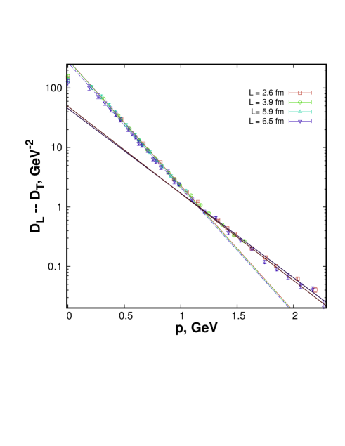
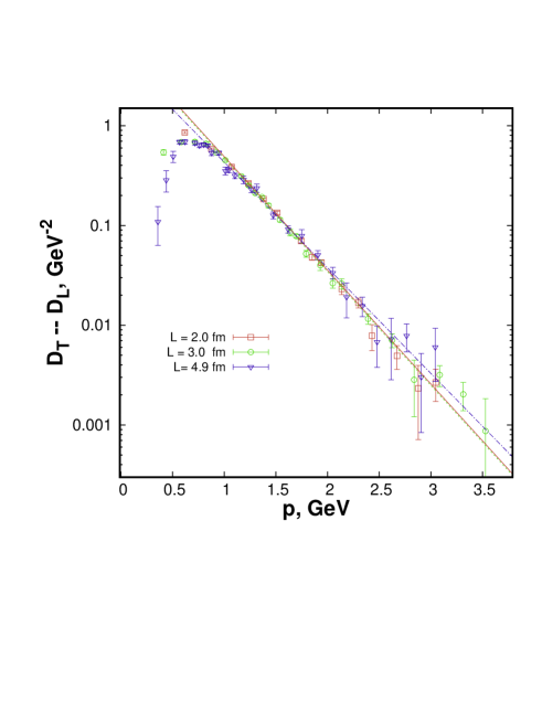
Figure 1: Dependence of $\Delta$ on $|\vec{p}|$ in the SU(2) theory at $T=1.014T_{c}$ (left panel) and $T=1.5T_{c}$ (right panel). Lines are the results of the fit by eq. (11). In the left panel we show the results of fitting by eq. (11) over two ranges: $0.2<|\vec{p}|<1.2$ GeV and $1.3<|\vec{p}|<2.2$ GeV.

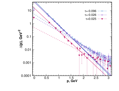
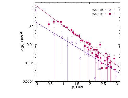
Figure 2: Dependence of $\Delta$ on $|\vec{p}|$ in the SU(3) theory: $T<T_{p}$ (left panel), $T>T_{p}$ (right panel). Lines are the results of the fit by formula (11).

Recently it was found Bornyakov et al. (2020); Bornyakov et al. (2021a) that the momentum dependence of the difference between the longitudinal and transverse propagators $\Delta(p)=D_{L}(p)-D_{T}(p)$ in dense quark matter can well be fitted by the function

$$\Delta(\vec{p})\simeq c\exp\Big{(}-\nu|\vec{p}|\Big{)}$$ (11)

over a sufficiently wide range of momenta. Here we study this fit in more details and find temperature dependence of the fit parameters $c$ and $\nu$ in SU(2) and SU(3) gluodynamics.

In Refs. Bornyakov et al. (2020); Bornyakov et al. (2021a) it was shown that the Gribov-Stingl fit function

$$D(p)=Z\;{M_{1}^{2}+p^{2}\over p^{4}+M_{2}^{2}\,p^{2}+M_{3}^{4}}\;.$$ (12)

works well for the longitudinal propagator, however, a poor quality of this fit in the case of the transverse propagator was found. Additionally it was found that the Gribov-Stingl fit for the transverse propagator is unstable with respect to an exclusion of the zero momentum. Thus, expression (11) should be helpful for finding an adequate fit function for the transverse gluon propagator.

It is reasonable to determine the parameters $M_{i}^{2}$ and $Z$ from the fit (12) to $D_{L}(p)$, the parameters $c$ and $\nu$ from the fit (11) to $\Delta(p)$ and consider the sum of the functions (12) and (11) with these parameters as an approximation to $D_{T}(p)$.

Typical dependence of $\Delta$ on $|\vec{p}|$ in the SU(2) theory is shown in Fig. 1 both at $T<T_{p}$ (left panel) and at $T>T_{p}$ (right panel). The results are presented for different lattice sizes to demonstrate that finite-volume effects in the domain of fitting are negligibly small. In the left panel it is seen that the dependence of $\Delta$ on the momentum abruptly changes at $p=p_{c}\sim 1.2$ GeV. However, $\Delta(\vec{p})$ can be fitted by eq. (11) both at $p<p_{c}$ and at $p>p_{c}$ with different sets of parameters $c$ and $\nu$ for different fitting ranges.

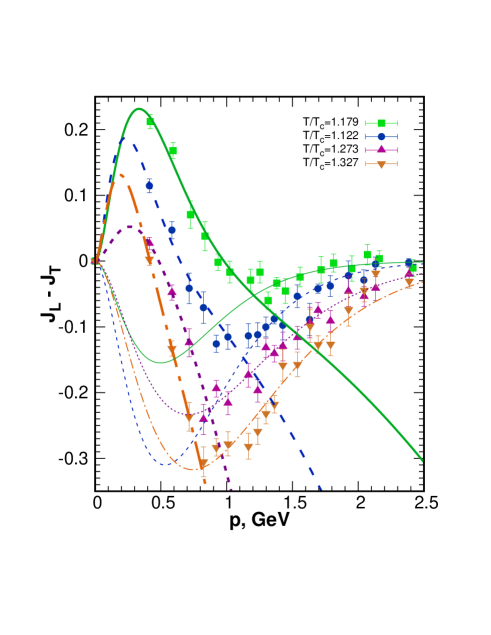
Figure 3: The behavior of the difference between the longitudinal and transverse gluon dressing functions in the vicinity of $T_{p}$ in the SU(2) theory. Bold lines are the results of the fit by formula (13) at $p<p_{c}$, thin lines — by formula (11) at $p>p_{c}$.

$\tau$	$ln|c|$	$\nu$	$p$-value
-0.099	5.220(15)	4.486(21)	0.03
-0.008	5.488(18)	4.640(25)	0.89
-0.001	5.573(19)	4.730(27)	0.64
0.002	5.626(20)	4.780(25)	0.33
0.005	5.585(27)	4.783(36)	0.68
0.008	5.727(21)	4.850(27)	0.98
0.014	5.693(24)	4.892(32)	1.00
0.025	5.818(29)	5.058(40)	1.00
0.034	5.741(33)	4.982(44)	1.00
0.054	6.177(51)	5.318(71)	0.71
0.106	3.052(65)	4.440(81)	0.66

Table 3: Parameters $c$ and $\nu$ from the fit formula (11) for $T<T_{p}$ (SU(2) theory).

$T/T_{c}$	$ln|c|$	$\nu$	$p$-value
1.217	0.33(23)	2.45(20)	0.68
1.273	1.05(15)	2.63(13)	0.38
1.327	1.35(13)	2.60(11)	0.24
1.494	1.94(5)	2.68(4)	0.82
1.826	1.78(4)	2.23(4)	0.16
2.324	1.58(5)	1.87(3)	0.21

Table 4: Parameters $c$ and $\nu$ from the fit formula (11) for $T>T_{p}$ (SU(2) theory).

$\tau$	$c$ (GeV${}^{-}2$)	$\nu$ (GeV${}^{-}1$)	$p$-value
-0.096	61.9(5.0)	4.33(9)	0.02
-0.026	48.7(8.6)	4.18(17)	0.01
0.025	17.3(2.7)	4.15(13)	0.80
0.104	-16.5(2.2)	4.10(12)	0.79

Table 5: Parameters $c$ and $\nu$ from the fit formula (11) in the SU(3) theory.

Similar results for the SU(3) theory are presented in Fig 2.

In the case of SU(2) theory, the behavior of $\Delta(\vec{p})$ at $T\sim T_{p}$ is shown in Fig. 3. To make it visible in the plot, we use the difference $J_{L}-J_{T}$ between the dressing functions $J_{L,T}(p)=p^{2}D_{L,T}(p)$ instead of $\Delta(\vec{p})$.

To describe the behavior of $\Delta(\vec{p})$ at $T\sim T_{p}$, we employ fit formula

$$\Delta(\vec{p})\simeq c\exp\Big{(}-\nu|\vec{p}|\Big{)}-b$$ (13)

at $p<p_{c}$ and (11) at $p>p_{c}$.

The parameters $c$ and $\nu$ obtained by fitting the formula (11) to the data are given in Tables 3 and 4 for SU(2) theory and in Table 5 for SU(3) theory.

In the case of SU(2) the results for $T>T_{p}$ and $T<T_{p}$ are shown separately because at $T<T_{p}$ we use the range of fitting $p<p_{c}$, whereas $p_{c}$ decreases at $T>T_{c}$ and we consider the range of fitting at $p>p_{c}$ as the main relevant. The range of fitting employed for these tables is $0.3$ GeV$<|\vec{p}|<1.1$ GeV at $T<T_{p}$ and $1.0$ GeV$<|\vec{p}|<3\div 4$ GeV at $T>T_{p}$. The results at the temperatures close of $T_{p}$ are not presented in these tables because the behavior of $\Delta(\vec{p})$ changes and the domain of validity of the fit formula (11) associated with an appropriate range of fitting also changes as is discussed in connection with Fig 3.

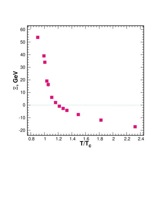
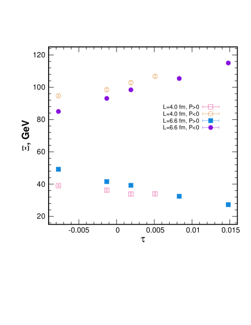
Figure 4: Left panel: temperature dependence of $\Xi$ in the SU(2) theory over the entire temperature range under consideration (for the sector ${\cal P}>0$). Right panel: temperature dependence of $\Xi$ at $T\approx T_{c}$ of $\Xi$ in different Polyakov-loop sectors and on a lattices of different size.

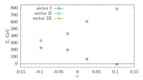
Figure 5: Temperature dependence of $\Xi$ in different center sectors for SU(3) theory at $T\sim T_{c}$.

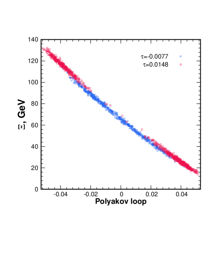
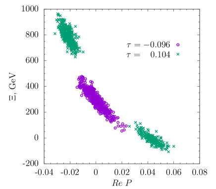
Figure 6: Correlations between $\Xi$ and the Polyakov loop: SU(2) theory (upper panel) and SU(3) theory (lower panel).

IV Integrated difference of the propagators

Since the difference between the propagators $\Delta(p)$ decreases rapidly with the momentum, it is reasonable to perform its integration with respect to the momentum in order to obtain a quantity sensitive to infrared dynamics of gauge fields. It should be emphasized that the asymmetry ${\cal A}$ can hardly be an indicator of infrared dynamics because it receives contributions from all momenta. Moreover, at $p_{4}=0$ the contribution of high momenta dominates over the contribution of low momenta. The ultraviolet convergence of ${\cal A}$ stems from cancellation of the high-$|\vec{p}|$ contributions at low $p_{4}$ and the contributions of high $p_{4}$.

In situations when the concept of potential is relevant and the interaction potential can be characterized by the Fourier transform of the propagator, the depth of the potential well is associated with the integral of the propagator over all momenta. Therefore, the integral of $\Delta(\vec{p},0)$ with respect to the 3-momentum characterizes the difference between the potentials of chromoelectric and chromomagnetic interactions.

Thus we define the Integrated Difference between the longitudinal and transverse Propagators (IDP) as follows

$$\Xi=\int d\vec{p}\big{(}D_{L}(\vec{p},0)-D_{T}(\vec{p},0)\big{)}\;.$$ (14)

It describes an overall contribution of infrared gluon dynamics to the difference between chromoelectric and chromomagnetic interactions. The IDP $\Xi$ is readily rearranged to the form

$$\Xi={(2\pi)^{3}T\over V(N_{c}^{2}-1)}\int d\vec{x}\int_{0}^{1/T}dx_{4}\int_{0}^{1/T}dy_{4}$$ (15)

$$\sum_{b=0}^{N_{c}}\Big{\langle}A_{4}^{b}(\vec{x},x_{4})A_{4}^{b}(\vec{x},y_{4})-{1\over 2}\sum_{i=1}^{3}A_{i}^{b}(\vec{x},x_{4})A_{i}^{b}(\vec{x},y_{4})\Big{\rangle}\;,$$

it can also be expressed in terms of lattice variables as follows:

$$\Xi={16\pi^{3}\beta T\over N_{s}^{3}N_{c}(N_{c}^{2}-1)}\;\sum_{\vec{x}}\!\sum_{x_{4},y_{4}}\!\sum_{b=1}^{3}$$ (16)

$$\left(\big{\langle}u_{4}^{b}(\vec{x},x_{4})u_{4}^{b}(\vec{x},y_{4})\big{\rangle}-{1\over 2}\sum_{i=1}^{3}\;\big{\langle}u_{i}^{b}(\vec{x},x_{4})u_{i}^{b}(\vec{x},y_{4})\big{\rangle}\right)$$

$x=(\vec{x},x_{4})\in\Lambda$ — $N_{s}^{3}\times N_{t}$ lattice.

In the free theory $\Delta=0$ and, therefore, $\Xi=0$. This contrasts with the asymmetry ${\cal A}$ (9), which in the free theory on a lattice can be recast to the form

$${\cal A}={2N_{c}(N_{c}^{2}-1)N_{t}\over 3\beta a^{2}N_{s}^{3}}\sum_{\hat{p}}{|\hat{\vec{p}}|^{2}-3\hat{p}_{4}^{2}\over 3(\hat{p}^{2})^{2}}$$ (17)

As is seen from this formula, the contribution of the $p_{4}=0$ mode to the asymmetry diverges when $a\to 0$ at high $\hat{p}_{i}$ and only the contributions of high-$p_{4}$ modes makes the asymmetry finite $\displaystyle{\cal A}\sim\;-\;{1\over 12}$ when $a\to 0$ Chernodub and Ilgenfritz (2008). For this reason, the IDP is better suited to characterize strength of interactions than the asymmetry, especially in the infrared domain. Yet another important difference between the IDP and the asymmetry is that $\Xi(T)$ goes through zero at some temperature, whereas ${\cal A}$ does not Bornyakov et al. (2016).

Temperature dependence of $\Xi$ in SU(2) theory in the center sector characterized by the positive values of the Polyakov loop is shown on the left panel of Fig. 4. It is clear that it goes through zero at $T\approx 1.2T_{c}$. At this temperature the longitudinal propagator associated with chromoelectric interactions becomes smaller than the transverse propagator associated with chromomagnetic interactions. This is not true for zero-momentum values of these propagators: $D_{L}(0)>D_{T}(0)$ even at substantially greater temperatures, however, the leading contribution to $\Xi$ comes from momenta $|\vec{p}|>200\div 400$ MeV, where $D_{T}>D_{L}$ at $T>T_{p}\approx 1.2T_{c}$. It should also be mentioned that $D_{T}(0)$ is plagued by the finite-volume and Gribov-copy effects and this fact hinders the determination of the temperature where $D_{L}(0)=D_{T}(0)$. Fortunately, the determination of such point is not very important since we have a useful quantity $\Xi$ reflecting the interplay between chromoelectric and chromomagnetic forces. At $T<T_{p}$ chromoelectric forces dominate: they are far-distant and sufficiently strong, which characterizes the postconfinement domain. However, with an increase of the chromoelectric mass they become screened at short distances so that chromomagnetic forces become dominating and we arrive at deconfined gluon matter. Thus $T_{p}$ should be considered as a natural boundary of the postconfinement domain. However, the question remains about gauge dependence of $T_{p}$.

It should be emphasized that $\Xi$ depends significantly on the center sector, its temperature dependence in different center sectors is shown in the right panel of Fig. 4.

A similar pattern takes place in the case of SU(3), it is shown in Fig. 5. In this case we obtain $T_{p}\approx 1.1T_{c}$. This value of the boundary of the postconfinement domain is substantially lower than that in Dumitru et al. (2011); Hidaka et al. (2015).

We also observe a significant correlation between $\Xi$ and ${\cal P}$, which is shown by the scatter plot in Fig. 6. Recently it was argued Bornyakov et al. (2021b) that such correlations imply similarity of critical behavior of the correlated quantities in the infinite-volume limit. Therefore, we expect that $\Xi(T)\sim\tau^{\beta}$ as $\tau\to 0_{+}$ in the case of SU(2) and $\Xi(T)$ has a discontinuity at $T=T_{c}$.

V Conclusions

We have studied the momentum and temperature dependence of the difference between the longitudinal and transverse propagators $\Delta(\vec{p},p_{4}=0;T)$.

Our findings can be summarized as follows:

• In a sufficiently wide range of infrared momenta $\Delta(\vec{p})$ can well be fitted by the function (11) and the parameter $c$ changes its sign at $T\simeq 1.2T_{c}$ in the SU(2) theory and at $T\simeq 1.1T_{c}$ in the SU(3) theory.

• In the center sector with a positive real part of the Polyakov-loop, the integrated difference of propagators $\Xi$ goes through zero at $T\simeq 1.2T_{c}$ in the SU(2) theory and at $T\simeq 1.1T_{c}$ in the SU(3) theory.

• The temperature $T_{p}$ at which $\Xi$ goes through zero can be considered as the boundary of the postconfinement domain, where chromoelectric interactions still dominate.

• A significant correlation between $\Xi$ and $\mathrm{Re}{\cal P}$ is observed indicating that these quantities have similar critical behavior.