Agent-Temporal Attention for Reward Redistribution in
Episodic Multi-Agent Reinforcement Learning

Abstract.

This paper considers multi-agent reinforcement learning (MARL) tasks where agents receive a shared global reward at the end of an episode. The delayed nature of this reward affects the ability of the agents to assess the quality of their actions at intermediate time-steps. This paper focuses on developing methods to learn a temporal redistribution of the episodic reward to obtain a dense reward signal. Solving such MARL problems requires addressing two challenges: identifying (1) relative importance of states along the length of an episode (along time), and (2) relative importance of individual agents’ states at any single time-step (among agents). In this paper, we introduce Agent-Temporal Attention for Reward Redistribution in Episodic Multi-Agent Reinforcement Learning (AREL) to address these two challenges. AREL uses attention mechanisms to characterize the influence of actions on state transitions along trajectories (temporal attention), and how each agent is affected by other agents at each time-step (agent attention). The redistributed rewards predicted by AREL are dense, and can be integrated with any given MARL algorithm. We evaluate AREL on challenging tasks from the Particle World environment and the StarCraft Multi-Agent Challenge. AREL results in higher rewards in Particle World, and improved win rates in StarCraft compared to three state-of-the-art reward redistribution methods. Our code is available at https://github.com/baicenxiao/AREL.

1. Introduction

Cooperative multi-agent reinforcement learning (MARL) involves multiple autonomous agents that learn to collaborate to complete tasks in a shared environment by maximizing a global reward (Busoniu et al., 2008). Examples of systems where MARL has been used include autonomous vehicle coordination Sallab et al. (2017), and video games (Samvelyan et al., 2019; Tampuu et al., 2017).

One approach to enable better coordination is to use a single centralized controller that can access observations of all agents Jiang and Lu (2018). In this setting, algorithms designed for single-agent RL can be used for the multi-agent case. However, this may not be feasible when trained agents are deployed independently or when communication costs between agents and the controller is prohibitive. In such a situation, agents will need to be able to learn decentralized policies.

The centralized training with decentralized execution (CTDE) paradigm, introduced in Lowe et al. (2017); Rashid et al. (2018), enables agents to learn decentralized policies efficiently. Agents using CTDE can communicate with each other during training, but are required to make decisions independently at test-time. The absence of a centralized controller will require each agent to assess how its own actions can contribute to a shared global reward. This is called the multi-agent credit assignment problem, and has been the focus of recent work in MARL, such as COMA Foerster et al. (2018), QMIX Rashid et al. (2018) and QTRAN Son et al. (2019). Solving the multi-agent credit assignment problem alone, however, is not adequate to efficiently learn agent policies when the (global) reward signal is delayed until the end of an episode.

In reinforcement learning, agents seek to solve a sequential decision problem guided by reward signals at intermediate time-steps. This is called the temporal credit assignment problem Sutton and Barto (2018). In many applications, rewards may be delayed. For example, in molecular design Olivecrona et al. (2017), Go Silver et al. (2016), and computer games such as Skiing Bellemare et al. (2013), a summarized score is revealed only at the end of an episode. The episodic reward implies absence of feedback on quality of actions at intermediate time steps, making it difficult to learn good policies. The long-term temporal credit assignment problem has been studied in single-agent RL by performing return decomposition via contribution analysis Arjona-Medina et al. (2019) and using sequence modeling Liu et al. (2019). These methods do not directly scale well to MARL since size of the joint observation space grows exponentially with number of agents Lowe et al. (2017).

Besides scalability, addressing temporal credit assignment in MARL with episodic rewards presents two challenges. It is critical to identify the relative importance of: i) each agent’s state at any single time-step (agent dimension); ii) states along the length of an episode (temporal dimension). We introduce Agent-Temporal Attention for Reward Redistribution in Episodic Multi-Agent Reinforcement Learning (AREL) to address these challenges.

AREL uses attention mechanisms Vaswani et al. (2017) to carry out multi-agent temporal credit assignment by concatenating: i) a temporal attention module to characterize the influence of actions on state transitions along trajectories, and; ii) an agent attention module, to determine how any single agent is affected by other agents at each time-step. The attention modules enable learning a redistribution of the episodic reward along the length of the episode, resulting in a dense reward signal. To overcome the challenge of scalability, instead of working with the concatenation of (joint) agents’ observations, AREL analyzes observations of each agent using a temporal attention module that is shared among agents. The outcome of the temporal attention module is passed to an agent attention module that characterizes the relative contribution of each agent to the shared global reward. The output of the agent attention module is then used to learn the redistributed rewards.

When rewards are delayed or episodic, it is important to identify ‘critical’ states that contribute to the reward. The authors of Gangwani et al. (2020) recently demonstrated that rewards delayed by a long time-interval make it difficult for temporal-difference (TD) learning methods to carry out temporal credit assignment effectively. AREL overcomes this shortcoming by using attention mechanisms to effectively learn a redistribution of an episodic reward. This is accomplished by identifying critical states through capturing long-term dependencies between states and the episodic reward.

Agents that have identical action and observation spaces are said to be homogeneous. Consider a task where two homogeneous agents need to collaborate to open a door by locating two buttons and pressing them simultaneously. In this example, while locations of the two buttons (states) are important, the identities of the agent at each button are not. This property is termed permutation invariance, and can be utilized to make the credit assignment process sample efficient Gangwani et al. (2020); Liu et al. (2019). Thus, a redistributed reward must identify whether an agent is in a ‘good’ state, and should also be invariant to the identity of the agent in that state. AREL enforces this property by designing the credit assignment network with permutation-invariant operations among homogeneous agents, and can be integrated with MARL algorithms to learn agent policies.

We evaluate AREL on three tasks from the Particle World environment Lowe et al. (2017), and three combat scenarios in the StarCraft Multi-Agent Challenge Samvelyan et al. (2019). In each case, agents receive a summarized reward only at the end of an episode. We compare AREL with three state-of-the-art reward redistribution techniques, and observe that AREL results in accelerated learning of policies and higher rewards in Particle World, and improved win rates in StarCraft.

2. Related Work

Several techniques have been proposed to address temporal credit assignment when prior knowledge of the problem domain is available. Potential-based reward shaping is one such method that provided theoretical guarantees in single Ng et al. (1999) and multi-agent Devlin and Kudenko (2011); Lu et al. (2011) RL, and was shown to accelerate learning of policies in Devlin et al. (2011). Credit assignment was also studied by incorporating human feedback through imitation learning Kelly et al. (2019); Ross et al. (2011) and demonstrations Brown et al. (2019); Huang et al. (2020).

When prior knowledge of the problem domain is not available, recent work has studied temporal credit assignment in single-agent RL with delayed rewards. An approach named RUDDER Arjona-Medina et al. (2019) used contribution analysis to decompose episodic rewards by computing the difference between predicted returns at successive time-steps. Parallelly, the authors of Liu et al. (2019) proposed using natural language processing models for carrying out temporal credit assignment for episodic rewards. The scalability of the above methods to MARL, though, can be a challenge due to the exponential growth in the size of the joint observation space Lowe et al. (2017).

In the multi-agent setting, recent work has studied performing multi-agent credit assignment at each time-step. Difference rewards were used to assess the contribution of an agent to a global reward in Agogino and Tumer (2006); Devlin et al. (2014); Foerster et al. (2018) by computing a counterfactual term that marginalized out actions of that agent while keeping actions of other agents fixed. Value decomposition networks, proposed in Sunehag et al. (2018), decomposed a centralized value into a sum of agent values to assess each one’s contributions. A monotonicity assumption on value functions was imposed in QMIX Rashid et al. (2018) to assign credit to individual agents. A generalized approach to decompose a joint value into individual agent values was presented in QTRAN Son et al. (2019). The Shapley Q-value was used in Wang et al. (2020) to distribute a global reward to identify each agent’s contribution. The authors of Yang et al. (2020) decomposed global Q-values along trajectory paths, while Zhou et al. (2020) used an entropy-regularized method to encourage exploration to aid multi-agent credit assignment. The above techniques did not address long-term temporal credit assignment and hence will not be adequate for learning policies efficiently when rewards are delayed.

Attention mechanisms have been used for multi-agent credit assignment in recent work. The authors of Mao et al. (2019) used an attention mechanism with a CTDE-based algorithm to enable each agent effectively model policies of other agents (from its own perspective). Hierarchical graph attention networks proposed in Ryu et al. (2020) modeled hierarchical relationships among agents and used two attention networks to effectively represent individual and group level interactions. The authors of Jiang et al. (2019); Liu et al. (2020a) combined attention networks with graph-based representations to indicate the presence and importance of interactions between any two agents. The above approaches used attention mechanisms primarily to identify relationships between agents at a specific time-step. They did not consider long-term temporal dependencies, and therefore may not be sufficient to learn policies effectively when rewards are delayed.

A method for temporal redistribution of episodic rewards in single and multi-agent RL was recently presented in Gangwani et al. (2020). A ‘surrogate objective’ was used to uniformly redistribute an episodic reward along a trajectory. However, this work did not use information from sample trajectories to characterize the relative contributions of agents at intermediate time-steps along an episode.

Our approach differs from the above-mentioned related work in that it uses attention mechanisms for multi-agent temporal credit assignment. AREL overcomes the challenge of scalability by analyzing observations of each agent using temporal and agent attention modules, which respectively characterize the effect of actions on state transitions along a trajectory and how each agent is influenced by other agents at each time-step. Together, these modules will enable an effective redistribution of an episodic reward. AREL does not require human intervention to guide agent behaviors, and can be integrated with MARL algorithms to learn decentralized agent policies in environments with episodic rewards.

3. Background

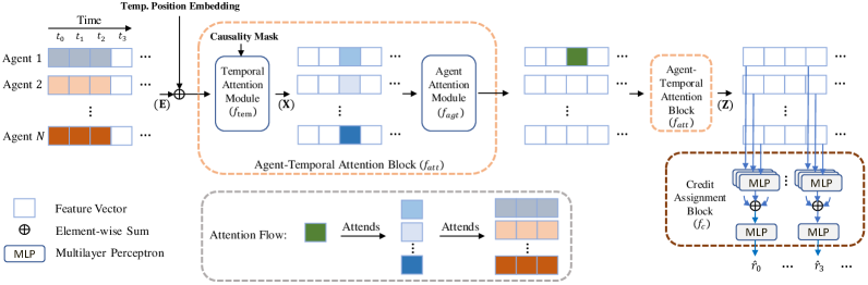
Figure 1. Schematic of AREL. The agent-temporal attention block concatenates temporal and agent attention modules, and summarizes input feature (e.g. observation) vectors. This is accomplished by establishing relationships between (attending to) information along time and among agents. The attention flow indicates that an output feature vector of the agent-temporal attention block for an agent at a time $t$ (green square) can attend to input features from all other agents before and including time $t$. Multiple agent-temporal attention blocks can be concatenated to each other to improve expressivity. The output of the last such block is fed to the credit assignment block, which applies shared multi-layer perceptrons to each attention feature. The output is the redistributed reward, which is integrated with MARL algorithms (e.g. MADDPG, QMIX) to learn agent policies.

A fully cooperative multi-agent task can be specified as a decentralized partially observable Markov decision process (Dec-POMDP) Oliehoek et al. (2016). A Dec-POMDP is a tuple $G=(S,A,P,r,Z,O,n,\gamma)$, where $s\in S$ describes the environment state. Each agent $i\in\{1,2,\dots,n\}$ receives an observation $o^{i}\in O^{i}$ according to an observation function $Z(s,i):S\times\mathbb{N}\rightarrow O$. At each time step, agent $i$ chooses action $a^{i}\in A^{i}$ according to its policy $\pi^{i}:O^{i}\times A^{i}\rightarrow[0,1]$. $A^{1}\times\dots\times A^{n}:=A$ forms the joint action space, and the environment transitions to the next state according to the function $P:S\times A^{1}\times\dots\times A^{n}\rightarrow S$. All agents share a global reward $r:S\times A\rightarrow\mathbb{R}$. The goal of the agents is to determine their individual policies to maximize the return, $J:=\mathbb{E}_{s\sim P,a^{1}\sim\pi^{1},\dots,a^{n}\sim\pi^{n}}[\sum_{t=0}^{T}\gamma^{t}r_{t}(s,a^{1},\dots,a^{n})]$, where $\gamma$ is a discount factor, and $T$ is the length of the horizon. Let $a_{t}:=(a^{1}_{t},\dots,a^{n}_{t})$ and $R_{t}:=\sum_{l=0}^{T-t}\gamma^{l}r_{t+1}$. A trajectory of length $T$ is an alternating sequence of observations and actions, $\tau:=(o_{0},a_{0},o_{1},a_{1},\dots,o_{T})$.

In a typical MARL task, agents receive reward $r(s,a)$ immediately following execution of action $a$ at state $s$. The expected return can then be determined by accumulating rewards at each time step. In episodic RL, a reward is revealed only at the end of an episode at time $T$, and agents do not receive a reward at intermediate time-steps. As a consequence, the expected return for all $t<T$ will be the same (when $\gamma=1)$. Therefore, the quality of information available for learning policies will be poor at all intermediate time steps. Moreover, delayed rewards have been shown to introduce a large bias Arjona-Medina et al. (2019) or variance Ng et al. (1999) in the performance of RL algorithms.

The CTDE paradigm Foerster et al. (2018); Lowe et al. (2017) can be adopted to learn decentralized policies effectively when dimensions of state and action spaces are large. During training, an agent can make use of information about other agents’ states and actions to aid its own learning. At test-time, decentralized policies are executed. This paradigm has been used to successfully complete tasks in complex MARL environments Gupta et al. (2017); Iqbal and Sha (2019); Rashid et al. (2018).

4. Approach

This paper considers MARL tasks where agents share the same global reward, which is received only at the end of an episode. The objective is to redistribute this episodic reward for effective multi-agent temporal credit assignment. To accomplish this goal, it is critical to identify the relative importance of: i) individual agents’ observations at each time-step, and; ii) observations along the length of a trajectory. We introduce AREL to address the above challenges. AREL uses an agent-temporal attention block to infer relationships among states at different times, and among agents. A schematic is shown in Fig. 1, and we describe its key components and overall workflow in the remainder of this section.

4.1. Agent-Temporal Attention

In order to redistribute an episodic reward in a meaningful way, we need to be able to extract useful information from trajectories. Each trajectory contains a sequence of observations involving all agents. At each time-step of an episode of length $T$, a feature of dimension $D$ corresponds to the embedding of a single observation. When there are $N$ agents, a trajectory is denoted by $\mathbf{E}\in\mathbb{R}^{T\times N\times D}$. The objective is to learn a mapping $f_{arel}(\mathbf{E}):\mathbb{R}^{T\times N\times D}\rightarrow\mathbb{R}^{T}$ to assign credit to the agents at each time-step. The information in a trajectory $\mathbf{E}$ comprises two parts: (1) temporal information between (embeddings of) observations at different time steps: this provides insight into the influence of actions on transitions between states; (2) structural information: this provides insight into how any single agent is affected by other agents.

These two parts are coupled, and hence studied together. The process of learning these relationships is termed attention. We propose an agent-temporal attention structure, inspired by the Transformer Vaswani et al. (2017). This structure selectively pays attention to different types of information- either from individual agents, or at different time-steps along a trajectory. This is accomplished by associating a weight to an observation based on its relative importance to other observations along the trajectory. The agent-temporal attention structure is formed by concatenating one agent attention module with one temporal attention module. The temporal attention modules determine how entries of $\mathbf{E}$ at different time-steps are related (along the ‘first’ dimension of $\mathbf{E}$). The agent attention module determines how agents influence one another (along the ‘second’ dimension of $\mathbf{E}$).

4.1.1. Temporal-Attention Module

The input is a trajectory $\mathbf{E}\in\mathbb{R}^{T\times N\times D}$. To calculate the temporal attention feature, we obtain the transpose of $\mathbf{E}$ as $\bar{\mathbf{E}}\in\mathbb{R}^{N\times T\times D}$. Adopting notation from Vaswani et al. (2017), each row $\mathbf{e}_{i}\in\mathbb{R}^{T\times D}$ of $\bar{\mathbf{E}}$ is transformed to a query $Q^{tem}_{i}:=\mathbf{e}_{i}W^{tem}_{q}$, key $K^{tem}_{i}:=\mathbf{e}_{i}W^{tem}_{k}$, and value $V^{tem}_{i}:=\mathbf{e}_{i}W^{tem}_{v}$. $W^{tem}_{q},W^{tem}_{k},W^{tem}_{v}\in\mathbb{R}^{D\times D}$ are learnable parameters, and $i\in\{0,\dots,N-1\}$. The $t^{th}$ row $x_{i,t}$ of the temporal attention feature $\mathbf{x}_{i}\in\mathbb{R}^{T\times D}$ is a weighted sum $x_{i,t}:=\alpha_{i,t}^{T}V^{tem}_{i}$. The attention weight vector $\alpha_{i,t}\in\mathbb{R}^{T\times 1}$ is a normalization (softmax) of the inner-product between the $t^{th}$ row of $Q^{tem}_{i}$, $q^{tem}_{i,t}$, and the key matrix $K^{tem}_{i}$:

$$\alpha_{i,t}^{T}=\text{softmax}(\frac{q^{tem}_{i,t}{K^{tem}_{i}}^{T}}{\sqrt{D}}\odot m^{T}_{t}),$$ (1)

where $\odot$ is an element-wise product, and $m_{t}$ is a mask with its first $t$ entries equal to $1$, and remaining entries $0$. The mask preserves causality by ensuring that at any time $t$, information beyond $t$ will not be used to assign credit. A temporal positional embedding Devlin et al. (2018) maintains information about relative positions of states in an episode. Position embeddings are learnable vectors associated to each temporal position of a trajectory. The sum of position and trajectory embeddings forms the input to the temporal attention module. The output of this module is $\mathbf{X}\in\mathbb{R}^{N\times T\times D}$, got by stacking $\mathbf{x}_{i},i\in{0,\dots,N-1}$. The temporal attention process can be described by a function $f_{tem}(\mathbf{E})\rightarrow\mathbf{X}$.

The output of the temporal attention module results in an assessment of each agent’s observation at any single time-step relative to observations at other time-steps of an episode. To obtain further insight into how an agent’s observation is related to other agents’ observations, an agent-attention module is concatenated to the temporal-attention module.

4.1.2. Agent-Attention Module

The agent-attention module uses the transpose of $\mathbf{X}$, denoted $\bar{\mathbf{X}}\in\mathbb{R}^{T\times N\times D}$. Each row of $\bar{\mathbf{X}}$, $\mathbf{x}_{t}\in\mathbb{R}^{N\times D}$ is transformed to a query $Q^{agt}_{t}=\mathbf{x}_{t}W^{agt}_{q}$, key $K^{agt}_{t}=\mathbf{x}_{t}W^{agt}_{k}$, and value $V^{agt}_{t}=\mathbf{x}_{t}W^{agt}_{v}$. Here, $W^{agt}_{q},W^{agt}_{k},W^{agt}_{v}\in\mathbb{R}^{D\times D}$ are learnable parameters. The $i^{th}$ row $z_{t,i}$ of the agent attention feature $\mathbf{z}_{t}\in\mathbb{R}^{N\times D}$ is a weighted sum, $z_{t,i}=\beta_{t,i}^{T}V^{agt}_{t}$. Maintaining causality is not necessary when computing the agent attention weight vector $\beta_{t,i}\in\mathbb{R}^{N\times 1}$. These weights are determined similar to the temporal attention weight vector in Eqn. (1), except without a masking operation. Therefore,

$$\beta_{t,i}^{T}=\text{softmax}(\frac{q^{agt}_{t,i}{K^{agt}_{t}}^{T}}{\sqrt{D}}).$$ (2)

The agent attention procedure can be described by a function $f_{agt}(\mathbf{X})\rightarrow\mathbf{Z}$, where $\mathbf{Z}\in\mathbb{R}^{T\times N\times D}$.

4.1.3. Concatenating Attention Modules

The output of the temporal attention module is an entity $\mathbf{X}$ that attends to information at time-steps along the length of an episode for each agent. Passing $\mathbf{X}$ through the agent attention module results in an output $\mathbf{Z}$ that is attended to by embeddings at all time-steps and from all agents. The data-flow of this process can be written as a composition of functions: $f_{att}:=f_{agt}\circ f_{tem}$. The temporal and agent attention modules can be repeatedly composed to improve expressivity. The position embedding is required only at the first temporal attention module when more than one is used.

4.2. Credit Assignment

The output of the attention modules is used to assign credit at each time-step along the length of the episode. Let $f_{arel}:=f_{c}\circ(f_{att}\circ\dots\circ f_{att})$, where $f_{c}:\mathbb{R}^{T\times N\times D}\rightarrow\mathbb{R}^{T}$. In order to carry out temporal credit assignment effectively, we leverage a property of permutation invariance.

4.2.1. Permutation Invariance

Agents sharing the same action and observation spaces are termed homogeneous. When homogeneous agents $ag1$ and $ag2$ cooperate to achieve a goal, the reward when $ag1$ observes $ob1$ and $ag2$ observes $ob2$ should be the same as the case when $ag1$ observes $ob2$ and $ag2$ observes $ob1$. This property is called permutation invariance, and has been shown to improve the sample-efficiency of multi-agent credit assignment as the number of agents increase Liu et al. (2020b); Gangwani et al. (2020). When this property is satisfied, the output of the function $f_{arel}$ should be invariant to the order of the agents’ observations. Formally, if the set of all permutations along the agent dimension (second dimension of $\mathbf{E}$) is denoted $\mathcal{H}$, then $f_{arel}(h_{1}(\mathbf{E}))=f_{arel}(h_{2}(\mathbf{E}))$ must be true for all $h_{1},h_{2}\in\mathcal{H}$.

The function $f_{att}$ is permutation invariant along the agent dimension by design. A sufficient condition for $f_{arel}$ to be permutation invariant is that the function $f_{c}$ be permutation invariant. To ensure this, we apply a multi-layer perceptron (MLP), add the MLP outputs element-wise, and pass it through another MLP. When functions $g_{1}$ and $g_{2}$ associated to the MLPs are continuous and shared among agents, the evaluation at time $t$ is the predicted reward $\hat{r}_{t}:=g_{2}\big{(}\sum_{i=0}^{N-1}g_{1}(z_{t,i})\big{)}$. It was shown in Zaheer et al. (2017) that any permutation invariant function can be represented by the above equation.

Remark 4.1.

AREL can be adapted to the heterogeneous case when cooperative agents are divided into homogeneous groups. Similar to a position embedding, we can apply an agent-group embedding such that agents within a group share an agent-group embedding. This will maintain permutation invariance of observations within a group, while enabling identification of agents from different groups. AREL will also work in the case when the multi-agent system is fully heterogeneous. This is equivalent to a scenario when there is only one agent in each homogeneous group. Therefore, AREL can handle agent types ranging from fully homogeneous to fully heterogeneous.

4.2.2. Credit Assignment Learning

Given a reward $R_{T}$ at the end of an episode of length $T$, the goal is to learn a temporal decomposition of $R_{T}$ to assess contributions of agents at each time-step along the trajectory. Specifically, we want to learn $\{\hat{r}_{t}\}_{t=0}^{T}$ satisfying $\sum_{t=0}^{T}\hat{r}_{t}=R_{T}$. Since $f_{arel}^{\theta}(\mathbf{E})$ is a vector in $\mathbb{R}^{T}$, its $t^{th}$ entry is denoted $f_{arel}^{\theta}(\mathbf{E}_{t})$ ($=\hat{r}_{t}$). The sequence $\{\hat{r}_{t}\}_{t=0}^{T}$ is learned by minimizing a regression loss, $l_{r}(\theta):=\mathbb{E}_{\mathbf{E,R_{T}}}\big{[}\frac{1}{T}\big{(}\sum_{t}(f_{arel}^{\theta}(\mathbf{E}_{t}))-R_{T}\big{)}^{2}\big{]}$, where $\theta$ are neural network parameters.

The redistributed rewards will be provided as an input to a MARL algorithm. We want to discourage $\{\hat{r}_{t}\}_{t=0}^{T}$ from being sparse, since sparse rewards may impede learning policies Devlin and Kudenko (2011). We observe that more than one combination of $\{\hat{r}_{t}\}_{t=0}^{T}$ can minimize $l_{r}(\theta)$. We add a regularization loss $l_{reg}(\theta)$ to select among solutions that minimize $l_{r}(\theta)$. Specifically, we aim to choose a solution that also minimizes the variance $l_{v}(\theta)$ of the redistributed rewards, and set $l_{reg}(\theta)=l_{v}(\theta)$ (we examine other choices of $l_{reg}(\theta)$ in the Appendix). Using $l_{v}(\theta)$ as a regularization term in the loss function leads to learning less sparsely redistributed rewards. With $\omega\in\mathbb{R}_{\geq 0}$ denoting a hyperparameter, the combined loss function used to learn $f_{arel}^{\theta}$ is:

$$loss_{total}(\theta)=l_{r}(\theta)+\omega l_{v}(\theta),$$ (3)

where $l_{v}(\theta):=\mathbb{E}_{\mathbf{E}}\big{[}\frac{1}{T}\sum_{t}(f_{arel}^{\theta}(\mathbf{E}_{t})-\bar{f}^{\theta}(\mathbf{E}))^{2}\big{]}$, and $\bar{f}^{\theta}(\mathbf{E}):=$
$\big{(}\sum_{t}f_{arel}^{\theta}(\mathbf{E}_{t})\big{)}/T$. The form of $loss_{total}(\theta)$ in Eqn. (3) incorporates the possibility that not all intermediate states will contribute equally to $R_{T}$, and additionally results in learning less sparsely redistributed rewards. Note that $\arg\min_{\theta}[loss_{total}(\theta)]$ will not typically yield $l_{r}(\theta)=l_{v}(\theta)=0$ (which corresponds to a uniform redistribution of rewards). Since some states may be common to different episodes, the redistributed reward $\hat{r}_{t}$ at each time-step cannot be arbitrarily chosen. For e.g., consider $N$ different episodes $\{E_{i}\}_{i=1}^{N}$, each of length $L$, with distinct cumulative episodic rewards $R_{i}$. If an intermediate state $s$ is common to episodes $E_{j}$ and $E_{k}$, under a uniform redistribution, distinct rewards $R_{j}/L$ and $R_{k}/L$ will be assigned to $s$, which is not possible. Thus, $l_{r}(\theta)=0$ and $l_{v}(\theta)=0$ will not both be true, implying that a uniform redistribution may not be viable.

4.3. Algorithm

Algorithm 1 AREL

0:  Number of agents $N$. Reward weight $\alpha\in[0,1]$. Initialize parameters $\theta,\phi$ for credit assignment and RL (policy/ critic) modules respectively. Experience buffer for storing trajectories $B_{e}\leftarrow\emptyset$. Prediction function update frequency $M$.

1:  for Episode $k=0,\dots$ do

2:     Reset episode return $R_{T}\leftarrow 0$; Reset trajectory for current episode $\tau\leftarrow\emptyset$

3:     for step $t=0,\dots,T-1$ do

4:        Sample action $a^{i}_{t}\sim\pi^{i}_{\phi}(o^{i}_{t})$, for $i=0,\dots,N-1$

5:        Take action $a_{t}$; Observe $o_{t+1}=(o^{0}_{t+1},\dots,o^{N-1}_{t+1})$

6:        Store transition $\tau\leftarrow\tau\cup\{(o_{t},a_{t},o_{t+1})\}$

7:     end for

8:     Update episode reward $R_{T}$; Store trajectory $B_{e}\leftarrow B_{e}\cup{(\tau,R_{T})}$

9:     Sample a batch of trajectories $B_{\tau}\sim B_{e}$

10:     Predict reward $\hat{r}_{t}$ using $f^{\theta}_{arel}(\tau)$ for each $\tau\in B_{\tau}$

11:     Update $\phi$ using $\{(o_{t},a_{t},o_{o_{t+1}})\}\in\tau$ and weighted reward $\alpha\hat{r}_{t}+(1-\alpha)\mathbf{1}_{t=T}R_{T}$

12:     if $k$ mod $M$ is 0 then

13:        for each gradient update do

14:           Sample a batch from $B_{e}$, and compute estimate of total loss, $\hat{loss}_{total}(\theta)$

15:           $\theta\leftarrow\theta-\nabla_{\theta}\hat{loss}_{total}(\theta)$

16:        end for

17:     end if

18:  end for

AREL is summarized in Algorithm 1. Parameters $\phi$ of RL modules and $\theta$ of the credit assignment function are randomly initialized. Observations and actions of agents are collected in each episode (Lines 2-6). Trajectories and episodic rewards are stored in an experience buffer $B_{e}$ (Line 8). The reward $\hat{r}_{t}$ at each time step for every trajectory in a batch $B_{\tau}$ (sampled from $B_{e}$) is predicted (Lines 9-10). The predicted $\hat{r}_{t}$ changes as $\theta$ is updated, but the episode reward $R_{T}$ remains the same. A weighted sum $\alpha\hat{r}_{t}+(1-\alpha)\mathbf{1}_{t=T}R_{T}$ ($\mathbf{1}_{t=T}$ is an indicator function) is used to update $\phi$ in a stable manner by using a MARL algorithm (Line 11). The credit assignment function $f_{arel}^{\theta}$ is updated when $M$ new trajectories are available (Lines 12-17).

4.4. Analysis

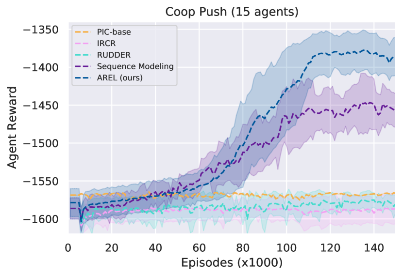
(a) Cooperative Push

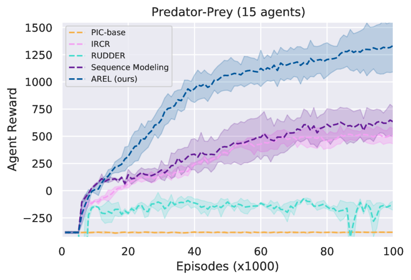
(b) Predator and Prey

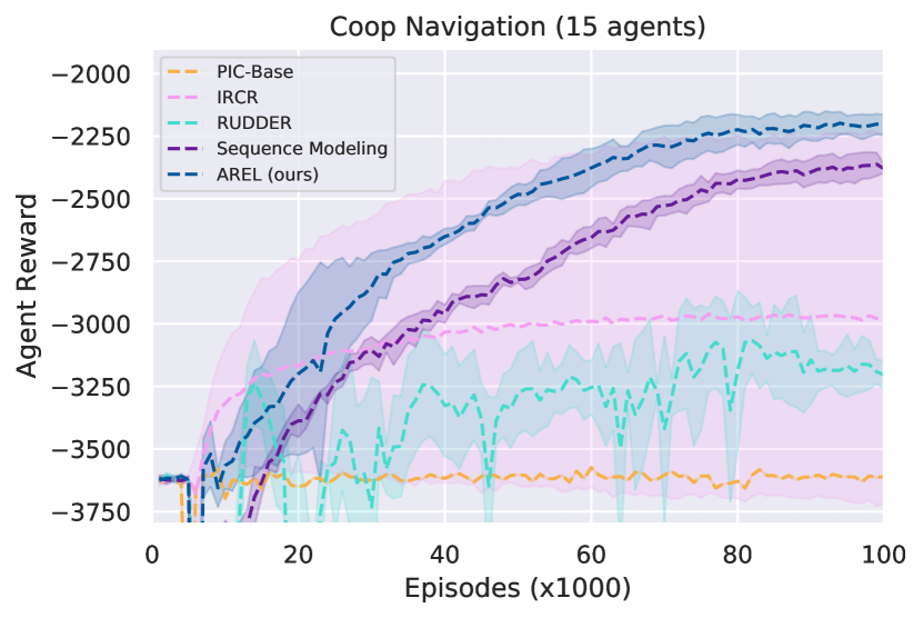
(c) Cooperative Navigation

Figure 2. Average agent rewards and standard deviation for tasks in Particle World with episodic rewards and $N=15$. AREL (dark blue) results in the highest average rewards in all tasks.

In order to establish a connection between redistributed rewards from Line 10 of Algorithm 1 and the episodic reward, we define return equivalence of decentralized partially observable sequence-Markov decision processes (Dec-POSDP). This generalizes the notion of return equivalence introduced in Arjona-Medina et al. (2019) in the fully observable setting for the single agent case. A Dec-POSDP is a decision process with Markov transition probabilities but has a reward distribution that need not be Markov. We present a result that establishes that return equivalent Dec-POSDPs will have the same optimal policies.

Definition 4.2.

Dec-POSDPs $\leavevmode\nobreak\ \tilde{\mathcal{P}}$ and $\mathcal{P}$ are return-equivalent if they differ only in their reward functions but have the same return for any trajectory $\tau$.

Theorem 4.3.

Given an initial state $s_{0}$, return-equivalent Dec-POSDPs will have the same optimal policies.

According to Definition 4.2, any two return equivalent Dec-POSDPs will have the same expected return for any trajectory $\tau$. That is, $\tilde{R}_{0}(\tau)=R_{0}(\tau),\forall\tau$. This is used to prove Theorem 4.3.

Proof.

Consider two return-equivalent Dec-POSDPs $\tilde{\mathcal{P}}$ and $\mathcal{P}$. Since $\tilde{\mathcal{P}}$ and $\mathcal{P}$ have the same transition probability and observation functions, the probabilities that a trajectory $\tau$ is realized will be the same if both Dec-POSDPs are provided with the same policy. For any joint agent policy $\pi:=(\pi^{1},\dots,\pi^{n})$ and sequence of states $s:=(s_{0},\dots,s_{T})$, we have:

$$\mathbb{E}_{\tau\sim(\pi,\tilde{Z},\tilde{P})} \big{[}\tilde{R}_{0}(\tau)\big{]}$$

$$=\sum_{\tau}\tilde{R}_{0}(\tau)\underbrace{\sum_{s}\tilde{p}(s_{0})\prod_{t=0}^{T-1}\pi(a_{t}|o_{t})\tilde{Z}(o_{t}|s_{t})\tilde{p}(s_{t+1}|s_{t},a_{t})}_{\tilde{p}^{\pi}(\tau)}$$

$$=\sum_{\tau}\tilde{R}_{0}(\tau)\underbrace{\sum_{s}p(s_{0})\prod_{t=0}^{T-1}\pi(a_{t}|o_{t})Z(o_{t}|s_{t})p(s_{t+1}|s_{t},a_{t})}_{p^{\pi}(\tau)}$$

$$=\sum_{\tau}R_{0}(\tau)\underbrace{\sum_{s}p(s_{0})\prod_{t=0}^{T-1}\pi(a_{t}|o_{t})Z(o_{t}|s_{t})p(s_{t+1}|s_{t},a_{t})}_{p^{\pi}(\tau)}$$

$$=\mathbb{E}_{\tau\sim(\pi,Z,P)}\big{[}R_{0}(\tau)\big{]}.$$

These equations follow from Definition 4.2. Let $\pi^{*}$ denote an optimal policy for $\tilde{\mathcal{P}}$. Then, we have:

$$\mathbb{E}_{\tau\sim(\pi^{*},\tilde{Z},\tilde{P})}\big{[}\tilde{R}_{0}(\tau)\big{]} =\mathbb{E}_{\tau\sim(\pi^{*},Z,P)}\big{[}R_{0}(\tau)\big{]}$$

$$\geq\mathbb{E}_{\tau\sim(\pi,\tilde{Z},\tilde{P})}\big{[}\tilde{R}_{0}(\tau)\big{]} =\mathbb{E}_{\tau\sim(\pi,Z,P)}\big{[}R_{0}(\tau)\big{]}.$$

Therefore, $\pi^{*}$ will also be an optimal policy for $\mathcal{P}$.∎

When $l_{r}(\theta)=0$ in Eqn. (3), a Dec-POSDP with the redistributed reward will be return-equivalent to a Dec-POSDP with the original episodic reward. Theorem 4.3 indicates that in this scenario, the two Dec-POSDPs will have the same optimal policies. An additional result in Appendix A gives a bound on $loss_{total}(\theta)$ when the estimators $f^{\theta}_{arel}(E_{t})$ are unbiased at each time-step.

5. Experiments

In this section, we describe the tasks that we evaluate AREL on, and present results of our experiments. Our code is available at https://github.com/baicenxiao/AREL.

5.1. Environments and Tasks

We study tasks from Particle World Lowe et al. (2017) and the StarCraft Multi-Agent Challenge Samvelyan et al. (2019). These have been identified as challenging multi-agent environments in Lowe et al. (2017); Samvelyan et al. (2019). In each task, a reward is received by agents only at the end of an episode. No reward is provided at other time steps. We briefly summarize the tasks below and defer detailed task descriptions to Appendix B.
(1) Cooperative Push: $N$ agents work together to move a large ball to a landmark.
(2) Predator-Prey: $N$ predators seek to capture $M$ preys. $L$ landmarks impede movement of agents.
(3) Cooperative Navigation: $N$ agents seek to reach $N$ landmarks. The maximum reward is obtained when there is exactly one agent at each landmark.
(4) StarCraft: Units from one group (controlled by RL agents) collaborate to attack units from another (controlled by heuristics). We report results for three maps: 2 Stalkers, 3 Zealots (2s3z); 1 Colossus, 3 Stalkers, 5 Zealots (1c3s5z); 3 Stalkers vs. 5 Zealots (3s_vs_5z).

5.2. Architecture and Training

In order to make the agent-temporal attention module more expressive, we use a transformer architecture with multi-head attention Vaswani et al. (2017) for both agent and temporal attention. The permutation invariant critic (PIC) based on the multi-agent deep deterministic policy gradient (MADDPG) from Liu et al. (2020b) is used as the base RL algorithm in Particle World. In StarCraft, we use QMIX Rashid et al. (2018) as the base RL algorithm. The value of $\alpha$ is set to $1$ in Particle World and $0.8$ in StarCraft. Additional details are presented in Appendix C.

5.3. Evaluation

We compare AREL with three state-of-the-art methods:
(1) RUDDER Arjona-Medina et al. (2019): A long short-term memory (LSTM) network is used for reward decomposition along the length of an episode.
(2) Sequence Modeling Liu et al. (2019): An attention mechanism is used for temporal decomposition of rewards along an episode.
(3) Iterative Relative Credit Refinement (IRCR) Gangwani et al. (2020): ‘Guidance rewards’ for temporal credit assignment are learned using a surrogate objective.

RUDDER and Sequence Modeling were originally developed for the single agent case. We adapted these methods to MARL by concatenating observations from all agents. We added the variance-based regularization loss in our experiments for Sequence Modeling, and observed that incorporating the regularization term resulted in an improved performance compared to without regularization.

5.4. Results

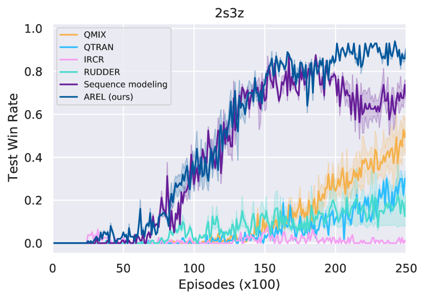
(a) 2s3z

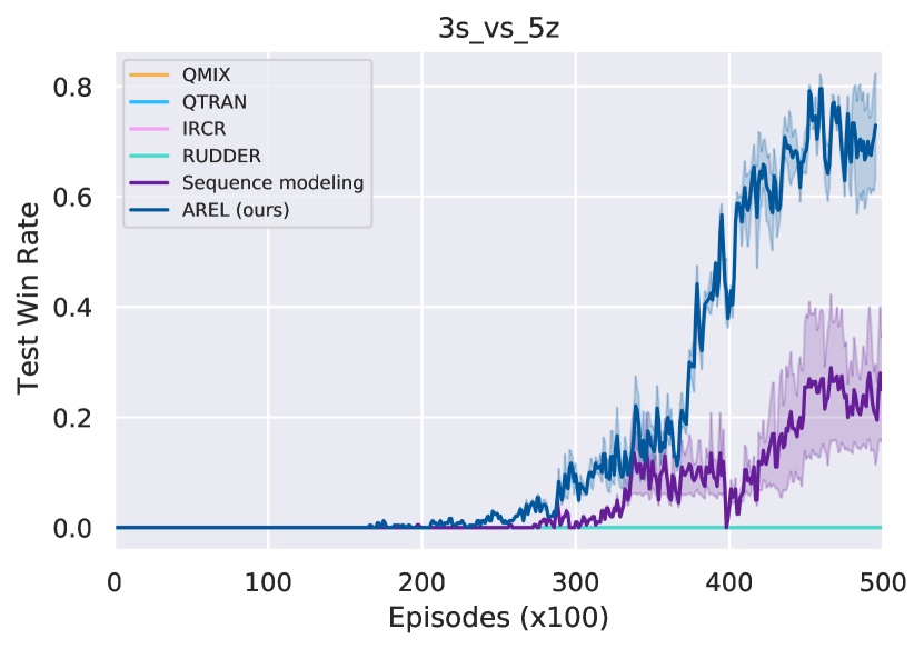
(b) 3s vs 5z

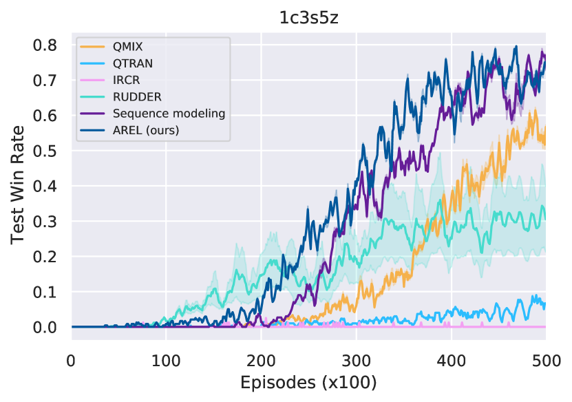
(c) 1c3s5z

Figure 3. Average test win rate and variance in StarCraft. AREL (dark blue) results in the highest win rates in 2s3z and 3s_vs_5z, and obtains a comparable win rate to Sequence Modeling in 1c3s5z.

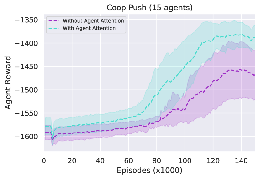
(a) Agent Attention

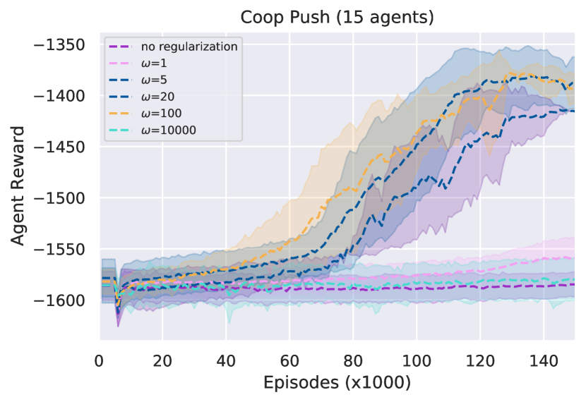
(b) Regularization

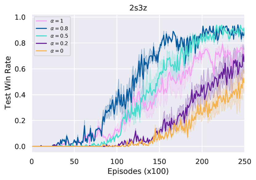
(c) Reward Weight

Figure 4. Ablations: Effects of the agent attention module (Fig. 4(a)) and regularization parameter $\omega$ in Eqn (3) (Fig. 4(b)) in Cooperative Push, and reward weight $\alpha$ (Fig. 4(c)) in the 2s3z StarCraft map.

5.4.1. AREL enables improved performance

Figure 2 shows results of our experiments for tasks in Particle World for $N=15$. In each case, AREL is able to guide agents to learn policies that result in higher average rewards compared to other methods. This is a consequence of using an attention mechanism to redistribute an episodic reward along the length of an episode, and also characterizing the contributions of individual agents.

The PIC baseline Liu et al. (2020b) fails to learn policies to complete tasks with episodic rewards. A similar result of failure to complete tasks was observed when using RUDDER Arjona-Medina et al. (2019). An explanation for this could be that RUDDER only carries out a temporal redistribution of rewards, but does not consider the effect of agents contributing differently to a reward.

Sequence Modeling Liu et al. (2019) performs better than RUDDER and the PIC baseline, possibly because it uses attention to redistribute episodic rewards. This was shown to outperform LSTM-based models, including RUDDER, in Liu et al. (2019) in single-agent episodic RL, due to the relative ease of training the attention mechanism. We believe that absence of an explicit characterization of agent-attention resulted in a lower reward for this method compared to AREL.

Using a surrogate objective in IRCR Gangwani et al. (2020) results in obtaining rewards comparable to AREL in some runs in the Cooperative Navigation task. However, the reward when using IRCR has a much higher variance compared to that obtained when using AREL. A possible reason for this is that IRCR does not characterize the relative contributions of agents at intermediate time-steps.

Figure 3 shows the results of our experiments for the three maps in StarCraft. AREL achieves the highest average win rate in the 2s3z and 3s_vs_5z maps, and obtains a comparable win rate to Sequence Modeling in 1c3s5z. Sequence Modeling does not explicitly model agent-attention, which could explain the lower average win rates in 2s3z and 3s_vs_5z. RUDDER achieves a nonzero, albeit much lower win rate than AREL in two maps, possibly because the increased episode length might affect the redistribution of the episode reward for this method. IRCR and QTRAN Son et al. (2019) obtain the lowest win rates. Additional experimental results are provided in Appendix D.

5.4.2. Ablations

We carry out several ablations to evaluate components of AREL. Figure 4(a) demonstrates the impact of the agent-attention module. In the absence of agent-attention (while retaining permutation invariance among agents through the shared temporal attention module), rewards are significantly lower. We study the effect of the value of $\omega$ in Eqn. (3) on rewards in Figure 4(b). This term is critical in ensuring that agents learn good policies. This is underscored by observations that rewards are significantly lower for very small or very large $\omega$ ($\omega=0,\omega=1,\omega=10000$). Third, we evaluate the effect of mixing the original episodic reward and redistributed reward by changing the reward weight $\alpha$ in Figure 4(c). The reward mixture influences win rates; $\alpha=$ 0.5 or 0.8 yields the highest win rate. The win rate is $\sim 10\%$ lower when using redistributed reward alone ($\alpha=1$). Additional ablations and evaluating the choice of regularization loss are shown in Appendices E and F.

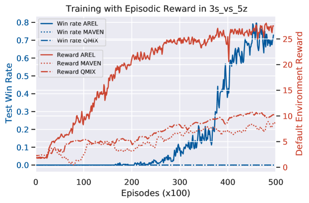
Figure 5. Comparison of AREL with QMIX and a strategic exploration technique, MAVEN in the $3s\_vs\_5z$ StarCraft map (avg. over 5 runs). AREL yields highest rewards and win rates.

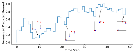
Figure 6. An instantiation of the Cooperative Navigation task with $N=3$ where rewards are provided only at the end of an episode. Blue and red dots respectively denote agents and landmarks. Arrows on agents represent their directions of movement. The objective of this task is for each agent to cover a distinct landmark. The $y-$axis of the graph shows the $0-1$ normalized predicted rewards for a sample trajectory. The positions of agents relative to landmarks are shown at several points along this trajectory. The figure shows a scenario where two agents are close to a single landmark. In this case, one of them must remain close to this landmark, while the other moves towards a different landmark. The predicted redistributed reward encourages such an action, since it has a higher magnitude when agents navigate towards distinct landmarks. The predicted redistributed reward by AREL is not uniform along the length of the episode.

5.4.3. Credit Assignment vs. exploration

This section demonstrates the importance of effective redistribution of an episodic reward vis-a-vis strategic exploration of the environment. The episodic reward $R_{T}(=\sum_{t}r_{t})$ takes continuous values and provides fine-grained information on performance (beyond only win/ loss). AREL learns a redistribution of $R_{T}$ by identifying critical states in an episode, and does not provide exploration abilities beyond that of the base RL algorithm. The redistributed rewards of AREL can be given as input to any RL algorithm to learn policies (in our experiments, we demonstrate using QMIX for StarCraft; MADDPG for Particle World). Figure 5 illustrates a comparison of AREL with a state-of-the-art exploration strategy, MAVEN Mahajan et al. (2019) and with QMIX Rashid et al. (2018) in the $3s\_vs\_5z$ StarCraft map. We observe that when rewards are delayed to the end of an episode, effectively redistributing the reward can be more beneficial than strategically exploring the environment to improve win-rates or total rewards.

5.4.4. Interpretability of Learned Rewards

Figure 6 presents an interpretation of the decomposed predicted rewards vis-a-vis the relative positions of agents to landmarks in the Cooperative Navigation task with $N=3$. When the reward is provided only at the end of an episode, AREL is used to learn a temporal redistribution of this episodic reward. The predicted rewards are normalized to a $0-1$ scale for ease of representation. The positions of the agents relative to the landmarks are shown at several points along a sample trajectory. Successfully trained agents must learn policies that enable each agent to cover a distinct landmark. For example, in a scenario where two agents are close to a single landmark, one of them must remain close to this landmark, while the other moves towards a different landmark. We observe that the magnitude of the predicted rewards is consistent with this insight in that it is higher when agents navigate away and towards different landmarks.

This visualization in Figure 6 reveals that the attention mechanism in AREL is able to learn to redistribute an episodic reward effectively in order to successfully train agents to accomplish task objectives in cooperative multi-agent reinforcement learning. Moreover, it reveals that the redistributed reward predicted by AREL is not uniform along the length of the episode.

5.5. Discussion

This paper focused on developing techniques to effectively learn policies in MARL environments when rewards were delayed or episodic. Our experiments demonstrate that AREL can be used as a module that enables more effective credit assignment by identifying critical states through capturing long-term temporal dependencies between states and an episodic reward. Redistributed rewards predicted by AREL are dense, which can then be provided as an input to MARL algorithms that learn value functions for credit assignment (we used MADDPG Lowe et al. (2017) and QMIX Rashid et al. (2018) in our experiments).

By including a variance-based regularization term, the total loss in Eqn. (3) enabled incorporating the possibility that not all intermediate states would contribute equally to an episodic reward, while also learning less sparse redistributed rewards. Moreover, any exploration ability available to the agents was provided solely by the MARL algorithm, and not by AREL. We further demonstrated that effective credit assignment was more beneficial than strategic exploration of the environment when rewards are episodic.

6. Conclusion

This paper studied the multi-agent temporal credit assignment problem in MARL tasks with episodic rewards. Solving this problem required addressing the twin challenges of identifying the relative importance of states along the length of an episode and individual agent’s state at any single time-step. We presented an attention-based method called AREL to deal with the above challenges. The temporally redistributed reward predicted by AREL was dense, and could be integrated with MARL algorithms. AREL was evaluated on tasks from Particle World and StarCraft, and was successful in obtaining higher rewards and better win rates than three state-of-the-art reward redistribution techniques.

7. Appendices

These appendices include detailed analysis and proofs of the theoretical results in the main paper. They also contain details of the environments and present additional experimental results and ablation studies.

Appendix A: Analysis

Using the variance of the predicted redistributed rewards as the regularization loss allows us to provide an interpretation of the overall loss in Eqn. (3) in terms of a bias-variance trade-off in a mean square estimator. The variance-regularized predicted rewards are analyzed in detail in the sequel.

First, assume that the episodic reward $R_{T}$ is given by the sum of ‘ground-truth’ rewards $r_{t}$ at each time step. That is, $R_{T}=\sum_{t}r_{t}$. The objective in Eqn. (3) is:

$$\arg\min_{\theta}loss_{total}(\theta) =\arg\min_{\theta}(l_{r}(\theta)+\omega l_{v}(\theta)).$$ (4)

This type of regularization will determine $f_{arel}^{\theta}$ in a manner such that it will be robust to overfitting.

For a sample trajectory, the expectation over $R_{T}$ in $l_{r}(\theta)$ can be omitted. Let $\bar{f}^{\theta}_{t}:=\mathbb{E}_{\mathbf{E}}(f_{arel}^{\theta}(\mathbf{E}_{t}))$ (i.e., the mean of the predicted rewards). Moreover, let $\bar{f}^{\theta}_{t}=\bar{f}^{\theta}(\mathbf{E}):=\frac{1}{T}\sum_{t}(f_{arel}^{\theta}(\mathbf{E}_{t}))$ (i.e., $\mathbf{E}_{t}$ is an ergodic process). Then, the following holds:

$$loss_{total}(\theta) =\mathbb{E}_{\mathbf{E}}\big{[}\frac{1}{T}\big{(}\sum_{t}(f_{arel}^{\theta}(\mathbf{E}_{t})-r_{t})\big{)}^{2}$$

$$\qquad\qquad+\frac{\omega}{T}\sum_{t}\big{(}f_{arel}^{\theta}(\mathbf{E}_{t})-\bar{f}^{\theta}_{t}\big{)}^{2}\big{]}$$ (5)

$$\leq\mathbb{E}_{\mathbf{E}}\big{[}\frac{1}{T}T\sum_{t}\big{(}f_{arel}^{\theta}(\mathbf{E}_{t})-r_{t}\big{)}^{2}$$

$$\qquad\qquad+\frac{\omega}{T}\sum_{t}\big{(}f_{arel}^{\theta}(\mathbf{E}_{t})-\bar{f}^{\theta}_{t}\big{)}^{2}\big{]}$$ (6)

The first term in (6) is obtained by applying the Cauchy-Schwarz inequality to the first term of (5). Consider $\mathbb{E}_{\mathbf{E}}[\sum_{t}\big{(}f_{arel}^{\theta}(\mathbf{E}_{t})-r_{t}\big{)}^{2}]$. From linearity of the expectation operator, this is equal to $\sum_{t}[\mathbb{E}_{\mathbf{E}}\big{(}f_{arel}^{\theta}(\mathbf{E}_{t})-r_{t}\big{)}^{2}]$. Then, $f_{arel}^{\theta}(\mathbf{E}_{t})$ can be interpreted as an estimator of $r_{t}$, and the expression above is the mean square error of this estimator. By adding and subtracting $\bar{f}^{\theta}_{t}$, the mean square error can be expressed as the sum of the variance and the squared bias of the estimator Domingos (2000). Formally,

$$\mathbb{E}_{\mathbf{E}}[\big{(}f_{arel}^{\theta}(\mathbf{E}_{t})-r_{t}\big{)}^{2}]=\mathbb{E}_{\mathbf{E}}[\big{(}f_{arel}^{\theta}(\mathbf{E}_{t})-\bar{f}^{\theta}_{t}+\bar{f}^{\theta}_{t}-r_{t}\big{)}^{2}]$$

$$=\mathbb{E}_{\mathbf{E}}[(f_{arel}^{\theta}(\mathbf{E}_{t})-\bar{f}^{\theta}_{t})^{2}+(\bar{f}^{\theta}_{t}-r_{t})^{2}+2(f_{arel}^{\theta}(\mathbf{E}_{t})-\bar{f}^{\theta}_{t})(\bar{f}^{\theta}_{t}-r_{t})].$$

After distributing the expectation in the above expression, we obtain the following:
(a): since $(\bar{f}^{\theta}_{t}-r_{t})$ is constant, the third term $\mathbb{E}_{\mathbf{E}}[(f_{arel}^{\theta}(\mathbf{E}_{t})-\bar{f}^{\theta}_{t})(\bar{f}^{\theta}_{t}-r_{t})]$ is equal to $(\bar{f}^{\theta}_{t}-r_{t})\mathbb{E}_{\mathbf{E}}[(f_{arel}^{\theta}(\mathbf{E}_{t})-\bar{f}^{\theta}_{t})]=(\bar{f}^{\theta}_{t}-r_{t})(\bar{f}^{\theta}_{t}-\bar{f}^{\theta}_{t})=0$;
(b): the first two terms correspond to the variance of a random variable $f_{arel}^{\theta}(\mathbf{E}_{t})$ and the square of a bias between $\bar{f}^{\theta}_{t}$ and $r_{t}$, and may not be both zero.
Substituting these in Eqn. (6),

$$loss_{total}(\theta) \leq\sum_{t}\big{[}(1+\frac{\omega}{T})\mathbb{E}_{\mathbf{E}}[(f_{arel}^{\theta}(\mathbf{E}_{t})-\bar{f}^{\theta}_{t})^{2}]$$

$$\qquad\qquad+\mathbb{E}_{\mathbf{E}}[(\bar{f}^{\theta}_{t}-r_{t})^{2}]\big{]}.$$ (7)

Therefore, the total loss is upper-bounded by an expression that represents the sum of a bias and a variance. The parameter $\omega$ will determine the relative significance of each term. Let $loss_{rhs}(\theta)$ represent the term on the right hand side of (7). If we denote by $\theta_{1}$ the parameters that minimize $loss_{total}(\theta)$, and by $\theta_{2}$ the parameters that minimize $loss_{rhs}(\theta)$, then an optimization carried out on $loss_{total}(\theta)$ can be related to one carried out on $loss_{rhs}(\theta)$ as:

$$loss_{total}(\theta_{1})\leq loss_{total}(\theta_{2})\leq loss_{rhs}(\theta_{2})\leq loss_{rhs}(\theta_{1}).$$

For the special case when the mean of the predicted rewards, $\bar{f}^{\theta}=\frac{R_{T}}{T}$, the first term of $loss_{total}(\theta)$ in Eqn. (5) will evaluate to zero. The optimization of $loss_{total}(\theta)$ in this case is then reduced to minimizing the square error of predictors $f^{\theta}_{arel}(E_{t})$ at each time $t\in\{0,1,\dots,T-1\}$. This setting is consistent with the principle of maximum entropy when the objective is to distribute an episodic return uniformly along the length of the trajectory.

Consider a single time-step $t_{1}$, and assume that there are enough samples (say, $S_{max}$) to ‘learn’ $f^{\theta}_{arel}(E_{t_{1}})$. Then, at each time-step $t_{1}$, the goal is to solve the problem $\mathbb{E}_{\theta}[(f^{\theta}_{arel}(E_{t_{1}})-\frac{R_{T}}{T})^{2}]$.

The squared loss above will admit a bias-variance decomposition Domingos (2000); Geman et al. (1992) that is commonly interpreted as a trade-off between the two terms. This underscores an insight that the complexity of the estimator (in terms of dimension of the set containing the parameters $\theta$) should achieve an ‘optimal’ balance Friedman et al. (2001); Goodfellow et al. (2016). This is represented as a U-shaped curve for the total error, where bias decreases and variance increases with the complexity of the estimator. However, recent work has demonstrated that the variance of the prediction also decreases with the complexity of the estimator Belkin et al. (2019); Neal et al. (2018).

In order to determine a bound on the error of the variance of the predictor at each time-step, we first state a result from Neal et al. (2018). We use this to provide a bound on $loss_{total}(\theta)$ when the estimators $f^{\theta}_{arel}(E_{t})$ are unbiased at each time-step in Theorem 7.2.

Theorem 7.1.

Neal et al. (2018) Let $N$ be the dimension of the parameter space containing $\theta$. Assume that the parameters $\theta$ are initialized by a Gaussian as $\theta_{0}\sim\mathcal{N}(0,\frac{1}{N}I)$. Let $L_{t_{1}}=o(\sqrt{N})$ be a Lipschitz constant associated to $f^{\theta}_{arel}(E_{t_{1}})$. Then, for some constant $C>0$, the variance of the prediction satisfies $Var_{\theta_{0}}(f^{\theta}_{arel}(E_{t_{1}}))\leq 2CL_{t_{1}}^{2}/N$.

Theorem 7.2.

Let $\bar{f}^{\theta}:=\mathbb{E}_{\mathbf{E}}(f_{arel}^{\theta}(\mathbf{E}))=R_{T}/T$ denote the mean of the predicted rewards. Assume that there are $S_{max}$ samples to ‘learn’ $f^{\theta}_{arel}(E_{t_{1}})$ at each time-step $t_{1}\in\{0,1,\dots,T-1\}$. Then, for unbiased estimators $f^{\theta}_{arel}(E_{t_{1}})$ and associated Lipschitz constants $L_{t_{1}}=o(\sqrt{N})$,

$$loss_{total}(\theta) \leq\frac{2\omega C}{NT}\sum_{t}(L_{0}^{2}+\dots L_{T-1}^{2}).$$

Proof.

The proof follows from applying Theorem 7.1 at each time step $t_{1}\in\{0,1,\dots,T-1\}$. Since the estimators at each time-step are unbiased, the mean square error of predictors $f^{\theta}_{arel}(E_{t})$ is equal to the variance of the predictor. The expectation operator in Eqn. (5) is now over a constant, which completes the proof. ∎

The assumption on estimators being unbiased is reasonable. Proposition 7.3 indicates that in the more general case (i.e. for an estimator that may not be unbiased), the prediction is concentrated around its mean with high probability.

Proposition 7.3.

Wainwright (2019) Under a Gaussian initialization of parameters as $\theta_{0}\sim\mathcal{N}(0,\frac{1}{N}I)$, at each time-step $t_{1}$, the following holds:

$$\mathbb{P}(|f^{\theta}_{arel}(E_{t_{1}})-\mathbb{E}_{\theta}[f^{\theta}_{arel}(E_{t_{1}})]|>\epsilon)\leq 2\leavevmode\nobreak\ exp(-\frac{CN\epsilon^{2}}{L^{2}}).$$

Theorem 7.2 indicates that the optimization of $loss_{total}(\theta)$ will be equivalent to minimizing the square error of predictors $f^{\theta}_{arel}(E_{t})$ at each time $t\in\{0,1,\dots,T-1\}$.

Appendix B: Detailed Task Descriptions

This Appendix gives a detailed description of the tasks that we evaluate AREL on. In each experiment, a reward is obtained by the agents only at the end of an episode. No reward is provided at other time steps.

• Cooperative Push: This task has $N$ agents working together to move a large ball to a landmark. Agents are rewarded when the ball reaches the landmark. Each agent observes its position and velocity, relative position of the target landmark and the large ball, and relative positions of the $k$ nearest agents. We report results for $(N,k)=(3,2)$, $(6,5)$, and $(15,10)$. At each time step, the distance $d^{t}_{a,b}$ between agents and the ball, distance $d^{t}_{b,l}$ between ball and landmark, and whether the agents touch the ball $I^{t}$ is recorded. These quantities, though, will be not be immediately revealed to the agents. Agents receive a reward $\sum_{t=1}^{T}(-\lambda_{1}d^{t}_{a,b}-\lambda_{2}d^{t}_{b,l}+\lambda_{3}I^{t})$ at the end of each episode at time $T$.

• Predator-Prey: This task has $N$ predators working together to capture $M$ preys. $L$ landmarks impede movement of the agents. Preys can move faster than predators, and predators obtain a positive reward when they collide with a prey. The $M$ prey agents are controlled by the environment. Each predator observes its position and velocity, relative locations of the $l$ nearest landmarks, and relative positions and velocities of the $k_{1}$ nearest prey and $k_{2}$ nearest predators. We report results for $(N,M,L,k_{1},k_{2},l)=(3,1,2,1,3,2)$, $(6,2,3,2,6,3)$, and $(15,5,5,3,6,3)$. At each time step, the distance $d^{t}_{prey,pred}$ between a prey and the closest predator, and whether a predator touches a prey $I^{t}$ is recorded. These quantities, though, will be not be immediately revealed to the agents. The agents receive a reward $\sum_{t=1}^{T}(-\lambda_{1}d^{t}_{prey,pred}+\lambda_{2}I^{t})$ at the end of each episode at time $T$.

• Cooperative Navigation: This task has $N$ agents seeking to reach $N$ landmarks. The maximum reward is obtained when there is exactly one agent at each landmark. Agents are also penalized for colliding with each other. Each agent observes its position, velocity, and the relative locations of the $k$ nearest landmarks and agents. We report results for $(N,k)=(3,2),(6,5),(15,5)$. At each time step, the distance $d^{t}_{a,l}$ between an agent and the closest landmark, and whether an agent collides with other agents $I^{t}$ is recorded. These quantities, though, will be not be immediately revealed to the agents. The agents receive a reward $\sum_{t=1}^{T}(-\lambda_{1}d^{t}_{a,l}-\lambda_{2}I^{t})$ at the end of each episode at time $T$.

• StarCraft: We use the SMAC benchmark from Samvelyan et al. (2019). The environment comprises two groups of army units, and units from one group (controlled by learning agents) collaborate to attack units from the other (controlled by handcrafted heuristics). Each learning agent controls one army unit. We report results for three maps: 2 Stalkers and 3 Zealots (2s3z); 1 Colossus, 3 Stalkers, and 5 Zealots (1c3s5z); and 3 Stalkers versus 5 Zealots (3s_vs_5z). In 2s3z and 1c3s5z, two groups of identical units are placed symmetrically on the map. In 3s_vs_5z, the learning agents control 3 Stalkers to attack 5 Zealots controlled by the StarCraft AI. In all maps, units can only observe other units if they are both alive and located within the sight range. The 2s3z and 1c3s5z maps comprise heterogeneous agents, since there are different types of units, while the 3s_vs_5z is a homogeneous map. In all our experiments, the default environment reward is delayed and revealed only at the end of an episode. The reader is referred to Samvelyan et al. (2019) for a detailed description of the default rewards.

Appendix C: Implementation Details

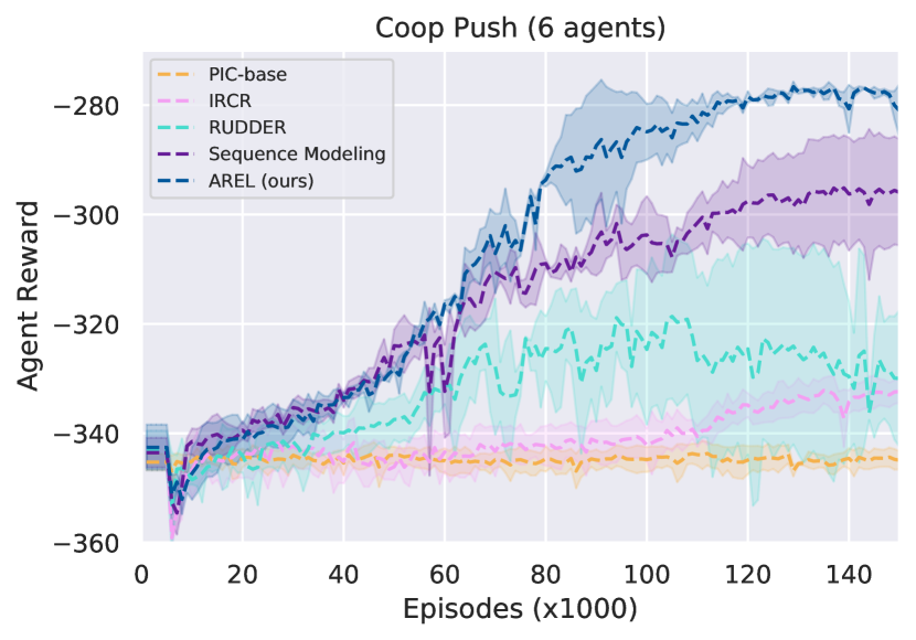
(a) Cooperative Push

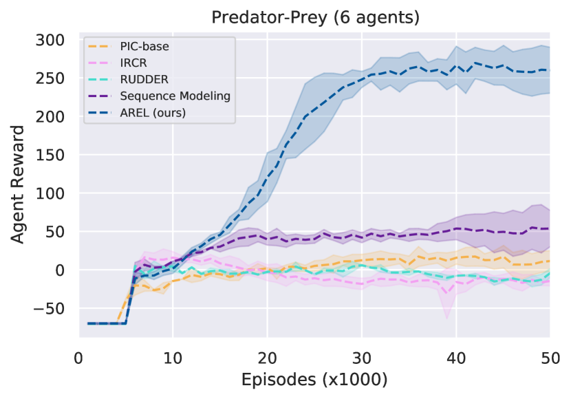
(b) Predator and Prey

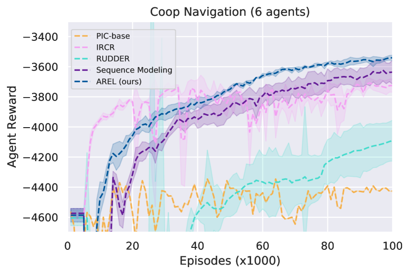
(c) Cooperative Navigation

Figure 7. Average agent rewards and standard deviation for tasks in the Particle World environment with episodic rewards and $N=6$. AREL (dark blue) results in the highest average rewards in all the tasks.

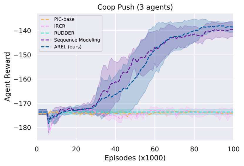
(a) Cooperative Push

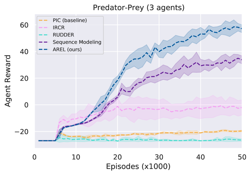
(b) Predator and Prey

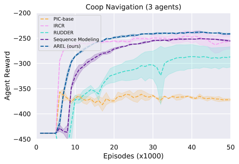
(c) Cooperative Navigation

Figure 8. Average agent rewards in Particle World environment with episodic rewards and $N=3$. AREL (dark blue) results in the highest average rewards.

All the results presented in this paper are averaged over 5 runs with different random seeds. We tested the following values for the regularization parameter in Eqn. (3): $\{0.1,1,10,20,50,100\}$, and observed that $\omega=20$ resulted in the best performance.

In order to make the agent-temporal attention module more expressive, we use a transformer architecture with multi-head attention Vaswani et al. (2017) for both agent and temporal attention. Specifically, in our experiments, the transformer architecture applies, in sequence: an attention layer, layer normalization, two feed forward layers with ReLU activation, and another layer normalization. Before each layer normalization, residual connections are added.

When dimension of the observation space exceeds $100$, a single fully connected layer with $100$ units is applied to compress the observation before attention module. The credit assignment block that produces redistributed rewards $\hat{r}_{t}$ consists of two MLPs, each with a single hidden layer of 50 units. Neural networks for credit assignment are trained using Adam with learning rate $1\times 10^{-4}$.

In Particle World, credit assignment networks are updated for $1000$ batches every $1000$ episodes. Each batch contains $256$ fully unrolled episodes uniformly sampled from the trajectory experience buffer $B_{e}$. In StarCraft, credit assignment networks are updated for $400$ batches every $200$ episodes. Each batch contains $32$ fully unrolled episodes uniformly sampled from $B_{e}$.

During training and testing, the length of each episode in Particle World is kept fixed at $25$ time steps, except in Predator-Prey with $N=15$, where the episode length is set to $50$ time steps. In StarCraft, an episode is restricted to have a maximum length of $120$ time steps for 2s3z, $180$ time steps for 1c3s5z, and $250$ time steps for 3s_vs_5z. If both armies are alive at the end of the episode, we count it as a loss for the team of learning agents. An episode terminates after one army has been defeated, or the time limit has been reached.

In Particle World, we use the permutation invariant critic (PIC) based on MADDPG from Liu et al. (2020b) as the base reinforcement learning algorithm. The code is based on the implementation available at https://github.com/IouJenLiu/PIC. Following MADDPG Lowe et al. (2017), the actor policy is parameterized by a two-layer MLP with 128 hidden units per layer, and ReLU activation function. The permutation invariant critic is a two-layer graph convolution net with 128 hidden units per layer, max pooling at the top, and ReLU activation. Learning rates for actor and critic are 0.01, and is linearly decreased to zero at the end of training. Trajectories of the first $5000$ episodes are sampled randomly for filling the experience buffer. During training, uniform noise was added for exploration during action selection.

In StarCraft, we use QMIX Rashid et al. (2018) as the base algorithm. The QMIX code is based on the implementation from https://github.com/starry-sky6688/StarCraft. In the implementation, all agent networks share a deep recurrent Q-network with recurrent layer comprised of a GRU with a 64-dimensional hidden state, with a fully-connected layer before and after. Trajectories of the first $20000$ episodes are sampled randomly to fill the experience buffer. Target networks are updated every 200 training episodes. QMIX is trained using RMSprop with learning rate $5\times 10^{-4}$. Throughout training, $\epsilon$-greedy is adopted for exploration, and $\epsilon$ is annealed linearly from 1.0 to 0.05 over 50k time steps and kept constant for the rest of learning.

The experiments that we perform in this paper require computational resources to train the attention modules of AREL in addition to those needed to train deep RL algorithms. Using these resources might result in higher energy consumption, especially as the number of agents grows. This is a potential limitation of the methods studied in this paper. However, we believe that AREL partially addresses this concern by sharing certain modules among all agents in order to improve scalability.

We provide a description of our hardware resources below:
Hardware Configuration: All our experiments were carried out on a machine running Ubuntu^®$18.04$ equipped with a $16-$core Intel^®Xeon^®$3.7$ GHz CPU, two NVIDIA^®GeFORCE^®RTX $2080$ Ti graphics cards and a $128$ GB RAM.

Appendix D: Additional Experimental Results

No. of Agents	Task	$R_{avg}$: AREL	$R_{avg}$: Uniform	$R_{final}$: AREL	$R_{final}$: Uniform
	CP	$\mathbf{-1490.7}$	-1553.6	$\mathbf{-1375.2}$	$-1477.6$
N = 15	PP	$\mathbf{827.7}$	$674.0$	$\mathbf{1325.0}$	$1167.0$
	CN	$\mathbf{-2691.1}$	$-2811.2$	$\mathbf{-2206.2}$	$-2301.1$
	CP	$\mathbf{-306.9}$	$-317.6$	$\mathbf{-282.4}$	$-286.3$
N = 6	PP	$\mathbf{149.4}$	$111.6$	$\mathbf{259.8}$	$229.7$
	CN	$\mathbf{-3902.3}$	$-3950$	$\mathbf{-3541.2}$	$-3648.6$
	CP	$\mathbf{-159.0}$	$-166.5$	$\mathbf{-139.2}$	$-146.1$
N = 3	PP	$\mathbf{23.4}$	$15.2$	$\mathbf{57.0}$	$46.9$
	CN	$\mathbf{-274.5}$	$-282.4$	$\mathbf{-241.5}$	$-244.4$

Table 1. Ablation: This table demonstrates the effect of removing the agent attention module, and uniformly weighting the attention of each agent in the three tasks in Particle World. This is termed Uniform, and we compare this with AREL. We report the average rewards over the number of training episodes ($R_{avg}$) and the final agent reward ($R_{final}$) at the end of training in both scenarios for each task. AREL consistently results in higher average and maximum rewards (shown in bold), which indicates that the agent attention module plays a crucial role in effective credit assignment.

This Appendix presents additional experimental results carried out in the Particle World environment.

Figure 7 shows results of our experiments for tasks in Particle World when $N=6$. In each case, AREL is consistently able to allow agents to learn policies that result in higher average rewards compared to other methods. This is a consequence of using an attention mechanism that enables decomposition of an episodic reward along the length of an episode, and that also characterizes contributions of individual agents to the reward. Performances of the PIC baseline Liu et al. (2020b), RUDDER Arjona-Medina et al. (2019), and Sequence Modeling Liu et al. (2019) can be explained similar to that presented for the case $N=15$ in the main paper. Using a surrogate objective in IRCR Gangwani et al. (2020) results in obtaining comparable agent rewards in some cases in the Cooperative Navigation task, but the reward curves are unstable and have high variance.

Figure 8 show the results of experiments on these tasks when $N=3$. The PIC baseline and RUDDER are unable to learn good policies and IRCR results in lower rewards than AREL in two tasks. The performance of Sequence Modeling is comparable to AREL, which indicates that characterizing agent attention plays a smaller role when there are fewer agents.

Appendix E: Additional Ablations

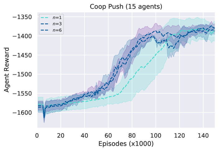
Figure 9. Ablation: Effect of the number of agent-temporal attention blocks on rewards.

This Appendix presents additional ablations that examine the impact of uniformly weighting the attention of agents and the number of agent-temporal attention blocks.

We evaluate the effect of removing the agent-attention block, and uniformly weighting the attention of each agent. This is termed uniform agent attention (Uniform). The average rewards over the number of training episodes ($R_{avg}$) and the final agent reward ($R_{final}$) at the end of training obtained when using AREL and when using Uniform are compared. The results of these experiments, presented in Table 1, indicate that $R_{avg}$ and $R_{max}$ are higher for AREL than for Uniform. This shows that the agent-attention block in AREL plays a crucial role in performing credit assignment effectively.

We examine the effect of the number of agent-temporal attention blocks, $n$ (depth) on rewards in the Cooperative Push task with $N=15$ in Figure 9. The depth has negligible impact on average rewards at the end of training. However, rewards during the early stages of training are lower for $n=1$, and these rewards also have a larger variance than the other cases ($n=3,6$).

Appendix F: Effect of Choice of Regularization Loss

This Appendix examines the effect of the choice of the regularization loss term in Eqn. (3). The need for the regularization loss term arises due to the possibility that there could be more than one choice of redistributed rewards that minimize the regression loss alone. In our results in the main paper, we used the variance of the redistributed rewards as the regularization loss. This choice was motivated by a need to discourage the predicted redistributed rewards from being sparse, since sparse rewards might impede learning of policies when provided as an input to a MARL algorithm Devlin and Kudenko (2011). By adding a variance-based regularization, the total loss enables incorporating the possibility that not all intermediate states would contribute equally to an episodic reward, while also resulting in learning redistributed rewards that are less sparse.

We compare the variance-based regularization loss with two other widely used choices of the regularization loss- the $L_{1}$ and $L_{2}$-based losses. The $L_{1}$-based regularization encourages learning sparse redistributed rewards, and the $L_{2}$-based regularization discourages learning a redistributed reward of large magnitude (i.e., ‘spikes’ in the redistributed reward). Specifically, we study:

$$loss_{total}(\theta) =l_{r}(\theta)+\omega l_{v}(\theta)$$

$$loss_{total}(\theta) =l_{r}(\theta)+\omega_{1}l_{1}(\theta)$$

$$loss_{total}(\theta) =l_{r}(\theta)+\omega_{2}l_{2}(\theta),$$

where $l_{r}(\theta),l_{v}(\theta)$ are the regression loss and variance of redistributed rewards as in Eqn. (3), $l_{1}(\theta)$ ($l_{2}(\theta)$) is the $L_{1}$ norm ($L_{2}$ norm) of the redistributed reward.

We compare the use of the three regularization loss functions on the tasks in Particle World with $N=15$. In each task, we calculate the $0-1$-normalized reward received by the agents during the last $1000$ training steps. We use $\omega=20$ for the variance-based regularization loss. For the other two regularization losses, we searched over $\omega_{1}\in\{0.1,1,10,100\}$ and $\omega_{2}\in\{0.1,1,10,100\}$, and we observed that $\omega_{1}=10$ and $\omega_{2}=10$ resulted in the best performance. The graph in Figure 10 shows the average $0-1$-normalized reward. We observe that using a variance-based regularization loss results in agents obtaining the highest average rewards.

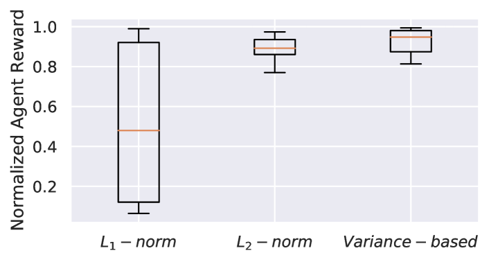
Figure 10. Normalized average agent rewards for tasks in Particle World when using variance-based, $L_{1}$-based, and $L_{2}$-based regularization losses. The variance-based regularization results in agents obtaining the highest average rewards.

In particular, we observe that using an $L_{1}$-based regularization results in significantly smaller rewards. A possible reason for this is that the $L_{1}$-based regularization has the property of encouraging learning a sparse redistributed reward, which hinders learning of policies when provided as an input to the MARL algorithm. The performance when using the $L_{2}$-based regularization results in a comparable, albeit slightly lower, average agent reward to using the variance-based regularization. This is reasonable since using the variance-based or $L_{2}$-based regularization will result in less sparse predicted redistributed rewards.

Appendix G: Verification of QMIX Implementation

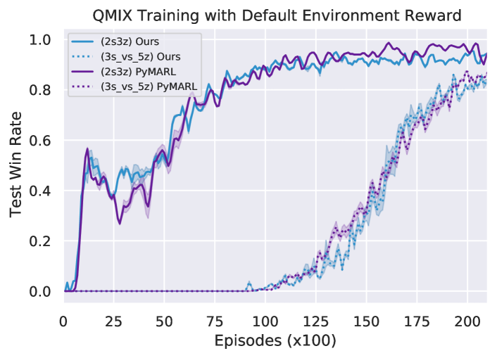
Figure 11. Comparison of PyMARL and our implementations (avg. over 5 runs). Test win-rates using either implementation are almost identical.

This Appendix demonstrates correctness of the QMIX implementation that we use from https://github.com/starry-sky6688/StarCraft. In the QMIX evaluation first used in Rashid et al. (2018), rewards were not delayed. In our experiments, rewards are delayed and revealed only at the end of an episode. In such a scenario, QMIX may not be able to perform long-term credit assignment, which explains the difference in performance between the default and delayed reward cases. We observe that using redistributed rewards from AREL as an input to QMIX results in an improved performance compared to using QMIX alone when rewards from the environment were delayed (Figure 3 in the main paper). Using the default, non-delayed rewards, we compare the performance of the QMIX implementation that we used in our experiments with the benchmark implementation from Samvelyan et al. (2019). Figure 11 shows that test win rates in two StarCraft maps ($2s3z$ and $3s\_vs\_5z$) using both implementations are almost identical.

References

- (1)
- Agogino and Tumer (2006) Adrian K Agogino and Kagan Tumer. 2006. QUICR-learning for multi-agent coordination. In Proceedings of the National Conference on Artificial Intelligence, Vol. 21. 1438.
- Arjona-Medina et al. (2019) Jose A Arjona-Medina, Michael Gillhofer, Michael Widrich, Thomas Unterthiner, Johannes Brandstetter, and Sepp Hochreiter. 2019. RUDDER: Return decomposition for delayed rewards. In Neural Information Processing Systems. 13566–13577.
- Belkin et al. (2019) Mikhail Belkin, Daniel Hsu, Siyuan Ma, and Soumik Mandal. 2019. Reconciling modern machine-learning practice and the classical bias–variance trade-off. Proceedings of the National Academy of Sciences 116, 32 (2019), 15849–15854.
- Bellemare et al. (2013) Marc G Bellemare, Yavar Naddaf, Joel Veness, and Michael Bowling. 2013. The Arcade Learning Environment: An evaluation platform for general agents. Journal of Artificial Intelligence Research 47 (2013), 253–279.
- Brown et al. (2019) Daniel Brown, Wonjoon Goo, Prabhat Nagarajan, and Scott Niekum. 2019. Extrapolating Beyond Suboptimal Demonstrations via Inverse Reinforcement Learning from Observations. In International Conference on Machine Learning.
- Busoniu et al. (2008) Lucian Busoniu, Robert Babuska, and Bart De Schutter. 2008. A comprehensive survey of multiagent reinforcement learning. IEEE Transactions on Systems, Man, and Cybernetics, Part C (Applications and Reviews) 38, 2 (2008), 156–172.
- Devlin et al. (2018) Jacob Devlin, Ming-Wei Chang, Kenton Lee, and Kristina Toutanova. 2018. BERT: Pre-training of deep bidirectional transformers for language understanding. arXiv preprint arXiv:1810.04805 (2018).
- Devlin and Kudenko (2011) Sam Devlin and Daniel Kudenko. 2011. Theoretical considerations of potential-based reward shaping for multi-agent systems. In International Conference on Autonomous Agents and Multi-Agent Systems. 225–232.
- Devlin et al. (2011) Sam Devlin, Daniel Kudenko, and Marek Grześ. 2011. An empirical study of potential-based reward shaping and advice in complex, multi-agent systems. Advances in Complex Systems 14, 02 (2011), 251–278.
- Devlin et al. (2014) Sam Devlin, Logan Yliniemi, Daniel Kudenko, and Kagan Tumer. 2014. Potential-based difference rewards for multiagent reinforcement learning. In International Conference on Autonomous Agents and Multi-Agent Systems. 165–172.
- Domingos (2000) Pedro Domingos. 2000. A unified bias-variance decomposition for zero-one and squared loss. AAAI/IAAI 2000 (2000), 564–569.
- Foerster et al. (2018) Jakob N Foerster, Gregory Farquhar, Triantafyllos Afouras, Nantas Nardelli, and Shimon Whiteson. 2018. Counterfactual multi-agent policy gradients. In AAAI Conference on Artificial Intelligence. 2974–2982.
- Friedman et al. (2001) Jerome Friedman, Trevor Hastie, and Robert Tibshirani. 2001. The Elements of Statistical Learning. Springer Series in Statistics.
- Gangwani et al. (2020) Tanmay Gangwani, Yuan Zhou, and Jian Peng. 2020. Learning Guidance Rewards with Trajectory-space Smoothing. In Neural Information Processing Systems.
- Geman et al. (1992) Stuart Geman, Elie Bienenstock, and René Doursat. 1992. Neural networks and the bias/variance dilemma. Neural computation 4, 1 (1992), 1–58.
- Goodfellow et al. (2016) Ian Goodfellow, Yoshua Bengio, Aaron Courville, and Yoshua Bengio. 2016. Deep Learning. MIT Press.
- Gupta et al. (2017) Jayesh K Gupta, Maxim Egorov, and Mykel Kochenderfer. 2017. Cooperative multi-agent control using deep reinforcement learning. In International Conference on Autonomous Agents and Multiagent Systems. 66–83.
- Huang et al. (2020) Sili Huang, Bo Yang, Hechang Chen, Haiyin Piao, Zhixiao Sun, and Yi Chang. 2020. MA-TREX: Multi-agent Trajectory-Ranked Reward Extrapolation via Inverse Reinforcement Learning. In International Conference on Knowledge Science, Engineering and Management. Springer, 3–14.
- Iqbal and Sha (2019) Shariq Iqbal and Fei Sha. 2019. Actor-attention-critic for multi-agent reinforcement learning. In International Conference on Machine Learning. 2961–2970.
- Jiang et al. (2019) Jiechuan Jiang, Chen Dun, Tiejun Huang, and Zongqing Lu. 2019. Graph Convolutional Reinforcement Learning. In International Conference on Learning Representations.
- Jiang and Lu (2018) Jiechuan Jiang and Zongqing Lu. 2018. Learning attentional communication for multi-agent cooperation. In Neural Information Processing Systems.
- Kelly et al. (2019) Michael Kelly, Chelsea Sidrane, Katherine Driggs-Campbell, and Mykel J Kochenderfer. 2019. HG-DAgger: Interactive Imitation Learning with Human Experts. In International Conference on Robotics and Automation. IEEE, 8077–8083.
- Liu et al. (2020b) Iou-Jen Liu, Raymond A Yeh, and Alexander G Schwing. 2020b. PIC: Permutation invariant critic for multi-agent deep reinforcement learning. In Conference on Robot Learning. 590–602.
- Liu et al. (2019) Yang Liu, Yunan Luo, Yuanyi Zhong, Xi Chen, Qiang Liu, and Jian Peng. 2019. Sequence Modeling of Temporal Credit Assignment for Episodic Reinforcement Learning. arXiv preprint arXiv:1905.13420 (2019).
- Liu et al. (2020a) Yong Liu, Weixun Wang, Yujing Hu, Jianye Hao, Xingguo Chen, and Yang Gao. 2020a. Multi-agent game abstraction via graph attention neural network. In Proceedings of the AAAI Conference on Artificial Intelligence, Vol. 34. 7211–7218.
- Lowe et al. (2017) Ryan Lowe, Yi I Wu, Aviv Tamar, Jean Harb, Pieter Abbeel, and Igor Mordatch. 2017. Multi-agent actor-critic for mixed cooperative-competitive environments. In Neural Information Processing Systems. 6379–6390.
- Lu et al. (2011) Xiaosong Lu, Howard M Schwartz, and Sidney Nascimento Givigi. 2011. Policy invariance under reward transformations for general-sum stochastic games. Journal of Artificial Intelligence Research 41 (2011), 397–406.
- Mahajan et al. (2019) Anuj Mahajan, Tabish Rashid, Mikayel Samvelyan, and Shimon Whiteson. 2019. MAVEN: Multi-agent variational exploration. arXiv preprint arXiv:1910.07483 (2019).
- Mao et al. (2019) Hangyu Mao, Zhengchao Zhang, Zhen Xiao, and Zhibo Gong. 2019. Modelling the Dynamic Joint Policy of Teammates with Attention Multi-agent DDPG. In Proceedings of the 18th International Conference on Autonomous Agents and MultiAgent Systems. 1108–1116.
- Neal et al. (2018) Brady Neal, Sarthak Mittal, Aristide Baratin, Vinayak Tantia, Matthew Scicluna, Simon Lacoste-Julien, and Ioannis Mitliagkas. 2018. A modern take on the bias-variance tradeoff in neural networks. arXiv preprint arXiv:1810.08591 (2018).
- Ng et al. (1999) Andrew Y Ng, Daishi Harada, and Stuart Russell. 1999. Policy invariance under reward transformations: Theory and application to reward shaping. In International Conference on Machine Learning. 278–287.
- Oliehoek et al. (2016) Frans A Oliehoek, Christopher Amato, et al. 2016. A concise introduction to decentralized POMDPs. Vol. 1. Springer.
- Olivecrona et al. (2017) Marcus Olivecrona, Thomas Blaschke, Ola Engkvist, and Hongming Chen. 2017. Molecular de-novo design through deep reinforcement learning. Journal of Cheminformatics 9, 1 (2017), 48.
- Rashid et al. (2018) Tabish Rashid, Mikayel Samvelyan, Christian Schroeder, Gregory Farquhar, Jakob Foerster, and Shimon Whiteson. 2018. QMIX: Monotonic Value Function Factorisation for Deep Multi-Agent Reinforcement Learning. In International Conference on Machine Learning. 4295–4304.
- Ross et al. (2011) Stéphane Ross, Geoffrey Gordon, and Drew Bagnell. 2011. A reduction of imitation learning and structured prediction to no-regret online learning. In International Conference on Artificial Intelligence and Statistics. 627–635.
- Ryu et al. (2020) Heechang Ryu, Hayong Shin, and Jinkyoo Park. 2020. Multi-agent actor-critic with hierarchical graph attention network. In Proceedings of the AAAI Conference on Artificial Intelligence, Vol. 34. 7236–7243.
- Sallab et al. (2017) Ahmad EL Sallab, Mohammed Abdou, Etienne Perot, and Senthil Yogamani. 2017. Deep reinforcement learning framework for autonomous driving. Electronic Imaging 2017, 19 (2017), 70–76.
- Samvelyan et al. (2019) Mikayel Samvelyan, Tabish Rashid, Christian Schroeder de Witt, Gregory Farquhar, Nantas Nardelli, Tim G. J. Rudner, Chia-Man Hung, Philiph H. S. Torr, Jakob Foerster, and Shimon Whiteson. 2019. The StarCraft Multi-Agent Challenge. CoRR abs/1902.04043 (2019).
- Silver et al. (2016) David Silver, Aja Huang, Chris J Maddison, Arthur Guez, Laurent Sifre, George Van Den Driessche, Julian Schrittwieser, Ioannis Antonoglou, Veda Panneershelvam, Marc Lanctot, Sander Dieleman, Dominik Grewe, John Nham, Nal Kalchbrenner, Ilya Sutskever, Timothy Lillicrap, Madeleine Leach, Koray Kavukcuoglu, Thore Graepel, and Demis Hassabis. 2016. Mastering the game of Go with deep neural networks and tree search. Nature 529, 7587 (2016).
- Son et al. (2019) Kyunghwan Son, Daewoo Kim, Wan Ju Kang, David Earl Hostallero, and Yung Yi. 2019. QTRAN: Learning to Factorize with Transformation for Cooperative Multi-Agent Reinforcement Learning. In International Conference on Machine Learning. 5887–5896.
- Sunehag et al. (2018) Peter Sunehag, Guy Lever, Audrunas Gruslys, Wojciech Marian Czarnecki, Vinícius Flores Zambaldi, Max Jaderberg, Marc Lanctot, Nicolas Sonnerat, Joel Z Leibo, Karl Tuyls, et al. 2018. Value-Decomposition Networks For Cooperative Multi-Agent Learning Based On Team Reward.. In International Conference on Autonomous Agents and Multiagent Systems. 2085–2087.
- Sutton and Barto (2018) Richard S Sutton and Andrew G Barto. 2018. Reinforcement Learning: An Introduction. MIT press.
- Tampuu et al. (2017) Ardi Tampuu, Tambet Matiisen, Dorian Kodelja, Ilya Kuzovkin, Kristjan Korjus, Juhan Aru, Jaan Aru, and Raul Vicente. 2017. Multiagent cooperation and competition with deep reinforcement learning. PloS One 12, 4 (2017), e0172395.
- Vaswani et al. (2017) Ashish Vaswani, Noam Shazeer, Niki Parmar, Jakob Uszkoreit, Llion Jones, Aidan N Gomez, Łukasz Kaiser, and Illia Polosukhin. 2017. Attention is all you need. In Neural Information Processing Systems. 5998–6008.
- Wainwright (2019) Martin J Wainwright. 2019. High-dimensional statistics: A non-asymptotic viewpoint. Cambridge University Press.
- Wang et al. (2020) Jianhong Wang, Yuan Zhang, Tae-Kyun Kim, and Yunjie Gu. 2020. Shapley Q-value: A local reward approach to solve global reward games. In Proceedings of the AAAI Conference on Artificial Intelligence, Vol. 34. 7285–7292.
- Yang et al. (2020) Yaodong Yang, Jianye Hao, Guangyong Chen, Hongyao Tang, Yingfeng Chen, Yujing Hu, Changjie Fan, and Zhongyu Wei. 2020. Q-value Path Decomposition for Deep Multiagent Reinforcement Learning. In International Conference on Machine Learning.
- Zaheer et al. (2017) Manzil Zaheer, Satwik Kottur, Siamak Ravanbhakhsh, Barnabás Póczos, Ruslan Salakhutdinov, and Alexander J Smola. 2017. Deep Sets. In Neural Information Processing Systems.
- Zhou et al. (2020) Meng Zhou, Ziyu Liu, Pengwei Sui, Yixuan Li, and Yuk Ying Chung. 2020. Learning Implicit Credit Assignment for Cooperative Multi-Agent Reinforcement Learning. In Neural Information Processing Systems.