Sensing performance enhancement via asymmetric gain optimization in the atom-light hybrid interferometer

Abstract

The SU (1,1)-type atom-light hybrid interferometer (SALHI) is a kind of interferometer that is sensitive to both the optical phase and atomic phase. However, the loss has been an unavoidable problem in practical applications and greatly limits the use of interferometers. Visibility is an important parameter to evaluate the performance of interferometers. Here, we experimentally demonstrate the mitigating effect of the loss on visibility of the SALHI via asymmetric gain optimization, where the maximum threshold of loss to visibility close to $100\%$ is increased. Furthermore, we theoretically find that the optimal condition for the largest visibility is the same as that for the enhancement of signal-to-noise ratio (SNR) to the best value with the existence of the losses using the intensity detection, indicating that visibility can act as an experimental operational criterion for SNR improvement in practical applications. Improvement of the interference visibility means achievement of SNR enhancement. Our results provide a significant foundation for practical application of the SALHI in radar and ranging measurements.

1 Introduction

Interferometers are widely used as sensors in precision measurement [1, 2, 3, 4]. There have been many kinds of interferometers, such as optical interferometers[5, 6, 7], atom interferometers[8, 9, 10, 11, 12, 13] and atom-light hybrid interferometer (ALHI)[14, 15]. Optical interferometers can measure the optical phase sensitive quantitation and are the core of optical gyroscopes[16], laser radar[17], ranging systems[18], etc. Atom interferometers can measure the atomic phase sensitive parameters, and have been demonstrated to measure the rotation rate[19], acceleration of gravity[20, 21, 22] and magnetic field[23, 24]. The ALHI is sensitive to both the optical and atomic phases, which has the potential to combine the advantages of optical wave and atomic systems in precision measurement, and has been utilized to measure angular velocity, electric field and magnetic field [14, 15, 25, 26].

In interferometry, the visibility represents the degree of interference cancellation of two beams, which can evaluate the performance of interferometers[27, 28, 29, 21, 12]. Low visibility has a negative effect on the measurement and causes a reduction in the SNR [30, 28, 31]. The SU(1, 1)-type interferometer realizes beam splitting and recombination through two parametric amplification processes[32, 27, 33, 34], whose two interference arms are quantum correlated. Comparing with conventional Mach-Zehnder interferometer (MZI), SNR of SU(1, 1)-type interferometer can break standard quantum limit due to quantum correlation. Previous literatures have shown that the SU(1, 1)-type interferometer has the tolerance to the detection loss (that is, external loss) by increasing the gain of the wave-recombination process [35, 36, 37, 38, 34] . However the SU(1, 1)-type interferometer, the internal loss has a greater effect on the perfect noise cancellation between two beams[39, 40]. Noise cancellation is the advantage of the SU(1, 1)-type interferometer[41]. The internal loss limit the practical application of the SU(1, 1)-type interferometer in radar and ranging measurements. Recently, in the presence of internal losses, augmenting the visibility through asymmetry is shown in the all optical SU(1, 1) interferometer [42], and here we extend to the case of SALHI.

In this paper, we experimentally and theoretically investigate the visibility optimization of SU(1, 1)-type ALHI (SALHI) with the existence of the internal loss. The conventional MZI is also given as a comparison. The visibility of SALHI and MZI decreases with the loss. However, we theoretically give an optimization condition, under which the visibility of SALHI ($\mathrm{{V_{SU}}}$) can be restored to ~100 $\%$ by optimizing the gain factor of wave recombination process to satisfy the optimization condition over a wide range of internal loss. In experiment $\mathrm{{V_{SU}}}$ is restored to $\sim$90$\%$. Furthermore, we theoretically analyze the SNR of the SALHI ($\mathrm{{SNR_{SU}}}$) and find that the optimization condition for $\mathrm{{SNR_{SU}}}$ enhancement is the same as that for the visibility restoration, which implies that as long as the $\mathrm{{V_{SU}}}$ is improved, the $\mathrm{{SNR_{SU}}}$ can be enhanced. In experiment, it is difficult to judge whether the experimental conditions are suitable to achieve the best $\mathrm{{SNR_{SU}}}$. However, the visibility is a physical quantity that is convenient to obtain and observe. Thus, the $\mathrm{{V_{SU}}}$ can be used as an experimental operational criterion for $\mathrm{{SNR_{SU}}}$ improvement. Therefore, the optimization condition and the $\mathrm{{V_{SU}}}$ restoration, have guiding significance for practical application of atom-light hybrid interferometers in the future.

2 SU(1, 1)-type atom-light hybrid interferometer

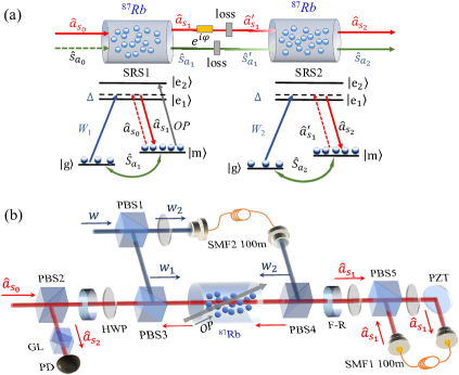
Figure 1: (a) Scheme of the SALHI, energy level of the ${}^{87}Rb$ atom, and frequencies of the laser. $\hat{a}_{s_{0}}$ and $\hat{S}_{a_{0}}$ are the initially input optical field and atomic spin wave, respectively. $\hat{a}_{s_{1}}$ and $\hat{S}_{a_{1}}$ are the interference arms generated from SRS1, which then evolve to $\hat{a}^{{}^{\prime}}_{s_{1}}$ and $\hat{S}^{{}^{\prime}}_{a_{1}}$ after loss and phase shift $\varphi$, finally becoming interference outputs $\hat{a}_{s_{2}}$ and $\hat{S}_{a_{2}}$ after SRS2. SRS: stimulated Raman scattering. $|g,m\rangle$: $|5^{2}S_{1/2},F=1,F=2\rangle$; $|e_{1},e_{2}\rangle$: $|5^{2}P_{1/2},F=2\rangle$, $|5^{2}P_{3/2}\rangle$; $W_{1}$ and $W_{2}$: Raman pump fields; OP: optical pumping field; $\Delta$: single photon detuning. (b) Experimental setup of the SALHI. PZT: piezoelectric transducer; PBS: polarization beam splitter; HWP: half-wave plate; F-R: Faraday rotator; GL: Glan prism; SMF: single-mode fiber; PD: photon detector. The diameters of $W_{1}$, $W_{2}$ and $\hat{a}_{s_{0}}$ are all 0.5mm.

The scheme of the SALHI is shown in Fig. 1 (a), where two stimulated Raman scattering processes, SRS1 and SRS2, are used to realize the wave splitting and recombination of optical field and atomic spin wave. SRS1 generates $\hat{a}_{s_{1}}$ and $\hat{S}_{a_{1}}$ acting as two interference arms of SALHI, and then SRS2 is used to recombine $\hat{a}^{{}^{\prime}}_{s_{1}}$ and $\hat{S}^{{}^{\prime}}_{a_{1}}$. The final interference outputs are optical signal $\hat{a}_{s_{2}}$ and atomic spin wave $\hat{S}_{a_{2}}$, respectively.

When SRS is operated in single mode, which can be realized by using the seed $\hat{a}_{s_{0}}$ and the $W$ beam in spatial single-mode from single-mode fiber in experiment. The Hamiltonian of SRS can be written as [43]

$$\hat{H}=i\hbar\zeta A_{W}\hat{a}^{\dagger}_{s}\hat{S}^{\dagger}_{a}+H.c,$$ (1)

where $\zeta=(g_{eg}g_{em})/\Delta$, with $g_{eg}$, $g_{em}$ are the coupling coefficients and $\Delta$ is the detuning frequency of the $W$ field as Fig. 1 (a) shown. $A_{W}$ is the amplitude of the strong $W$ field. The input-output relationship of SRS1 is

$$\begin{split}\hat{a}_{s_{1}}&=&G_{1}\hat{a}_{s_{0}}+g_{1}\hat{S}_{a_{0}}^{\dagger},\\ \hat{S}_{a_{1}}&=&G_{1}\hat{S}_{a_{0}}+g_{1}\hat{a}_{s_{0}}^{\dagger},\end{split}$$ (2)

where $\hat{a}_{s_{0}}$ and $\hat{S}_{a_{0}}$ are the initially input states of the optical field and atomic spin wave, respectively. $\hat{a}_{s_{0}}$ is the coherent state, and $\hat{S}_{a_{0}}$ is the vacuum state. Between SRS1 and SRS2, a phase shift $\varphi$, internal loss $l$ of the optical field, the dephasing $\eta$ of the atomic spin wave are introduced. Then, $\hat{a}_{s_{1}}$ becomes $\hat{a}_{s_{1}}^{{}^{\prime}}=\sqrt{1-l}\hat{a}_{s_{1}}e^{i\varphi}+\sqrt{l}\hat{v}$, and $\hat{S}_{a_{1}}$ becomes $\hat{S}_{a_{1}}^{{}^{\prime}}=\sqrt{1-\eta}\hat{S}_{a_{1}}+\sqrt{\eta}\hat{F},$ where $\hat{v}$ and $\hat{F}$ are the operators of vacuum. After the SRS2 process, the interference outputs are

$$\begin{split}\hat{a}_{s_{2}}=&(G_{1}G_{2}\sqrt{1-l}e^{i\varphi}+g_{1}g_{2}\sqrt{1-\eta})\hat{a}_{s_{0}}+G_{2}\sqrt{l}\hat{v}\\ +&(G_{2}g_{1}\sqrt{1-l}e^{i\varphi}+G_{1}g_{2}\sqrt{1-\eta})\hat{S}_{a_{0}}^{\dagger}+g_{2}\sqrt{\eta}\hat{F}^{\dagger},\\ \hat{S}_{a_{2}}=&(G_{1}g_{2}\sqrt{1-l}e^{-i\varphi}+G_{2}g_{1}\sqrt{1-\eta})\hat{a}_{s_{0}}^{\dagger}+g_{2}\sqrt{l}\hat{v}^{\dagger}\\ +&(g_{1}g_{2}\sqrt{1-l}e^{-i\varphi}+G_{1}G_{2}\sqrt{1-\eta})\hat{S}_{a_{0}}+G_{2}\sqrt{\eta}\hat{F},\end{split}$$ (3)

where the Raman gain factors $G_{k}=\frac{1}{2}(e^{\zeta_{k}A_{W}}+e^{-\zeta_{k}A_{W}})$ and $g_{k}=\frac{1}{2}(e^{\zeta_{k}A_{W}}-e^{-\zeta_{k}A_{W}})$ are related to $A_{W}$ and $\Delta$ of the $W$ field. $k=1,2$ represents SRS1 and SRS2, respectively. $G_{k}$ and $g_{k}$ satisfy $G_{k}^{2}-g_{k}^{2}=1$. The outputs $\hat{a}_{s_{2}}$ and $\hat{s}_{a_{2}}$ both depend on the gain factors, the losses $l$, $\eta$ and the phase shift.

3 Experimental setup

The experiment is performed in a cylindrical paraffin-coated ${}^{87}\!Rb$ vapor cell (diameter 0.5 cm, length 5 cm). As shown in Fig. 1(b), which was mounted inside a five-layer magnetic shield to reduce the stray magnetic field and heated to $75^{\circ}$C. Before the SRS1, almost all atoms are prepared in the ground state $|g\rangle$ by an optical pumping field (OP) resonant at the $|m\rangle$ $\rightarrow$ $|e_{2}\rangle$ transition. The OP pulse is 45 $\mu$s long, and its intensity is 110 mW. The $W$ field is divided into $W_{1}$ and $W_{2}$. $W_{2}$ is coupled into a 100 m-long single-mode fiber (SMF2). $W_{1}$ and initial input Stokes seed $\hat{a}_{s_{0}}$ are spatially overlapped by PBS3 and interact the atoms via SRS1. The detuning frequency $\Delta$ of $W$ is 1.2 GHz. The $\hat{a}_{s_{0}}$ beam is red tuned 6.8 GHz from the $W$ laser by an electro-optic modulator (EOM, Newport model No. 4851). After SRS1, $\hat{S}_{a_{1}}$ stays in the cell. $W_{1}$ and $\hat{a}_{s_{1}}$ exit the cell and are separated by PBS4. $\hat{a}_{s_{1}}$ is coupled into 100 m-long SMF1 and then returned back into the atomic cell with the $W_{2}$ pulse to interfere with $\hat{S}_{a_{1}}$ via SRS2. $\hat{a}_{s_{1}}$ and $W_{2}$ are temporally and spatially overlapped. The phase shift $\varphi$ of $\hat{a}_{s_{1}}$ is controlled by the PZT. The optical interference output $\hat{a}_{s_{2}}$ is detected by a photodetector after a Glan prism to filter $W_{2}$. In experiment, the internal loss $l$ of the optical interference beam is approximately 0.6, including the coupling efficiency of fiber, the transmittance of vapor cell and optical devices. The decay of the atomic spin wave is 0.4 due to atoms collisions and flying out of the interacting region during the evolution time between two SRS processes.

Comparing to optical MZI, whose two interference arms are both optical waves and the output is only sensitive to the optical phase, the SALHI goes one step futher relying atom-photon correlation. Thus the interference fringes depends on both atomic and optical phases.

4 Visibility results

In the experiment, we first measured the $\mathrm{{V_{SU}}}$ and the visibility of MZI ($\mathrm{{V_{MZ}}}$) with the same phase-sensitive particle number and internal loss as a comparison. Fig. 2 (a) shows the interference fringes of the Mach-Zehnder interferometer (MZI) and SALHI at $l$=0.96, $G_{1}=3$, $G_{2}=5$ and atomic decay rate $\eta=0.4$ of $\hat{S}_{a_{1}}$. The values of the $\mathrm{{V_{MZ}}}$ and $\mathrm{{V_{SU}}}$ are 45 $\%$ and 53 $\%$, respectively. Fig. 2 (b) shows the visibility value as a function of the loss rate $l$. In general, as the optical loss $l$ of $\hat{a}_{s_{1}}$ increases from 0.6 to 0.96 by variable attenuation plate, $\mathrm{V_{SU}}$ drops from 92.1$\%$ to 53$\%$, and $\mathrm{V_{MZ}}$ is always smaller than $\mathrm{V_{SU}}$ under the same loss condition.

In theory, according to Eq. (3), the visibility of the optical interference output $\hat{a}_{s_{2}}$ can be calculated and simplified as

$$\mathrm{V_{SU}}\approx\dfrac{2G_{1}G_{2}g_{1}g_{2}\sqrt{1-l}\sqrt{1-\eta}}{G_{1}^{2}G_{2}^{2}(1-l)+g_{1}^{2}g_{2}^{2}(1-\eta)}.$$ (4)

$\mathrm{V_{SU}}$ depends not only on the gain factors ($G_{1}$, $g_{1}$, $G_{2}$, $g_{2}$) but also on the internal losses $\left(\eta,l\right)$. The gain factors can be controlled by SRS parameters, such as the single-photon detuning $\Delta$ and power of $W$ fields. We give the theoretical visibility values obtained by using corresponding experimental parameters ($G_{1}$, $g_{1}$, $G_{2}$, $g_{2}$, $\eta$, $l$) shown in fig. 2 (b) with blue solid lines. The theoretical predictions and experimental data match well.

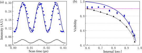
Figure 2: (a) The blue squares are the interference fringes of the SALHI with fixed $G_{1}$ =3, $G_{2}$ =5, $l$ =0.96 and $\eta$ =0.4, and the black triangles are the interference fringes of the MZI under the same operating conditions. (b) The visibility value as a function of the loss rate $l$. The blue squares represent $\mathrm{{V_{SU}}}$ with fixed $G_{1}$ = $3$, $G_{2}$ = $5$ and $\eta$ = $0.4$, the blue solid curve is the result of theoretical fitting according to Eq. (4), and the black triangles are the values of $\mathrm{V_{MZ}}$ measured experimentally. The pink dashed line corresponds to a visibility of 90$\%$.

5 Optimization condition

Furthermore, the largest interference visibility in Eq. (4) appears at

$$G_{1}G_{2}\sqrt{1-l}=g_{1}g_{2}\sqrt{1-\eta}.$$ (5)

We call this the optimization condition. According to Eqs. (2, 3), the interference output $\hat{a}_{s_{2}}$ consists of two parts. One is $G_{2}\hat{a}_{s_{1}}^{{\acute{}}}$ amplified from the optical arm $\hat{a}_{s_{1}}^{{{}^{\prime}}}=\sqrt{1-l}\hat{a}_{s_{1}}$, and the other is $g_{2}\hat{S}_{a_{1}}^{{\acute{}}}$ amplified from the atomic arm $\hat{S}_{a_{1}}^{{{}^{\prime}}}=\sqrt{1-\eta}\hat{S}_{a_{1}}$. When the gain factor of the wave-recombination process ($G_{2}$) is adjusted to satisfy the $G_{1}G_{2}\sqrt{1-l}=g_{1}g_{2}\sqrt{1-\eta}$, the amplitudes of the two parts are equal, then the visibility of output $\hat{a}_{s_{2}}$ can reach $\sim$100$\%$.

The SNR is also an important parameter to characterize the performance of an interferometer and can be calculated by SNR=$\dfrac{[(\partial\langle\hat{O}\rangle/\partial\varphi)\delta]^{2}}{\langle(\Delta\hat{O})^{2}\rangle}$[44, 45], where $\hat{O}$ is the measurable operator, $\delta$ is the added modulation small phase and $\langle(\Delta\hat{O})^{2}\rangle=\langle\hat{O}^{2}\rangle-\langle\hat{O}\rangle^{2}$. Under ID, the $\mathrm{{SNR_{SU}}}$ for the output optical field is

$$\mathrm{SNR_{SU}}\approx\dfrac{4G_{1}^{2}G_{2}^{2}g_{1}^{2}g_{2}^{2}(1-l)(1-\eta)N_{\hat{a}_{s_{0}}}sin^{2}\varphi\delta^{2}}{A^{2}(A^{2}+B^{2}+C^{2})},$$ (6)

where the input particle number $N_{\hat{a}_{s_{0}}}$= $\langle\hat{a}_{s_{0}}^{+}\hat{a}_{s_{0}}\rangle$, $A^{2}$ = $G_{1}^{2}G_{2}^{2}(1-l)+g_{1}^{2}g_{2}^{2}(1-\eta)\\ +2G_{1}G_{2}g_{1}g_{2}\sqrt{1-l}\sqrt{1-\eta}cos\varphi$, $B^{2}$ = $G_{2}^{2}g_{1}^{2}(1-l)+G_{1}^{2}g_{2}^{2}(1-\eta)+2G_{1}G_{2}g_{1}g_{2}\sqrt{1-l}\sqrt{1-\eta}cos\varphi$, and $C^{2}$ = $G_{2}^{2}l+g_{2}^{2}\eta$. $\mathrm{{SNR_{SU}}}$ is also related to internal losses $\left(\eta,l\right)$ and gain factors ($G_{1}$, $g_{1}$, $G_{2}$, $g_{2}$). To find the best $\mathrm{{SNR_{SU}}}$ condition under a certain loss $l$, we calculate the partial derivative

$$\dfrac{\partial(\mathrm{{SNR_{SU}})}}{\partial\sqrt{1-l}}=0.$$ (7)

When the interferometer operates near the dark point, that is, $\varphi=\pi+\Delta\varphi$ and $\Delta\varphi\sim 0$, the solution of Eq. (7) is $G_{1}G_{2}\sqrt{1-l}=g_{1}g_{2}\sqrt{1-\eta}$, where the best $\mathrm{{SNR_{SU}}}$ can be achieved.

Obviously, this condition for the $\mathrm{{SNR_{SU}}}$ under ID is same as Eq. (5), indicating that the improvement of $\mathrm{{V_{SU}}}$ corresponds to enhancement of $\mathrm{{SNR_{SU}}}$. The optimization condition is the key point to improve $\mathrm{{V_{SU}}}$ and enhance $\mathrm{{SNR_{SU}}}$ even at large internal loss. It should be noted that the interference visibility can be restored to $\sim 100\%$ and $\mathrm{{SNR_{SU}}}$ can be enhanced to the best value in the presence of losses when the experimental conditions satisfy the optimization condition. In the interferometer, phase shift can be measured using ID and balance homodyne detection (BHD). We also give the optimization condition for BHD in appendix part, which is different to Eq. (5).

To show the improvement of the SALHI compared with the conventional MZI under the same operating conditions, we calculated $\mathrm{{SNR_{MZ}}}$=$\dfrac{(1-l)(1-\eta)N_{0}sin^{2}\varphi\delta^{2}}{[(2-l-\eta)-2\sqrt{1-l}\sqrt{1-\eta}cos\varphi]}$[46, 47], where $N_{0}=(2G^{2}_{1}-1)N_{\hat{a}_{s_{0}}}$ is the phase-sensitive particle number of the MZI. Figs. 3 (a-c) shows the visibility and Figs. 3 (d-f) shows the SNR as a function of the optical loss $l$. Firstly, before optimization, as the loss $l$ increases, the $\mathrm{{SNR_{SU}}}$ first increase to a maximum value at $l=l_{B}$ and then decrease. In fact, $l_{B}$ is the point satisfying the optimization condition $G_{1}G_{2}\sqrt{1-l}=g_{1}g_{2}\sqrt{1-\eta}$, and compared with MZI, the quantum interferometers has better visibility. However, Figs. 3 (d-f) shows that $\mathrm{{SNR_{SU}}}$ is larger than $\mathrm{{SNR_{MZ}}}$ only within a small $l$ range near $l_{B}$ under a certain $G_{1}$, $G_{2}$ and $\eta$, and as $G_{1}$ and $\eta$ increase, this range is gradually diminished. The reason is that the increased $G_{1}$ or internal loss will bring more uncorrelated excess noise and quickly reduce the noise cancellation advantage of the SU(1, 1)-type interferometer. Therefore, when $G_{1}$, $g_{1}$ and $\eta$ are fixed, finding a suitable $G_{2}$ satisfying the optimization condition at each $l$ is an effective way to enhance $\mathrm{{SNR_{SU}}>{SNR_{MZ}}}$ over a wider range of internal loss.

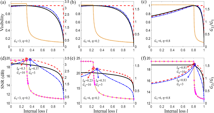
Figure 3: (a-c) The $\mathrm{{V_{SU}}}$ before and after optimization of the output field $\hat{a}_{s_{2}}$ and $\mathrm{{V_{MZ}}}$ as a function of $l$ (left-hand vertical axis). The blue dash-dotted curve is $\mathrm{{V_{SU}}}$ before optimization with fixed gain factors $G_{1}$, $g_{1}$, $G_{2}$, and $g_{2}$. The red dashed curve is largest $\mathrm{{V_{SU}}}$ (right-hand vertical axis) after optimizing $G_{2}$. The orange dotted curve is the value of $G_{2}/G_{1}$ after optimizing $G_{2}$ for the largest $\mathrm{{V_{SU}}}$, the black solid line is $\mathrm{{V_{MZ}}}$. (d-f) The black solid is $\mathrm{{SNR_{MZ}}}$ and the blue dash-dotted curves is $\mathrm{{SNR_{SU}}}$ before optimization with fixed gain factors $G_{1}$, $g_{1}$, $G_{2}$, and $g_{2}$, respectively, the red dashed curve is $\mathrm{{SNR_{SU}}}$ after optimizing $G_{2}$ (left-hand vertical axis). The pink circles represent the $G_{2}/G_{1}$ value at the best $\mathrm{{SNR_{SU}}}$ after optimization, and the orange dotted curve is the $G_{2}/G_{1}$ value of the largest $\mathrm{{V_{SU}}}$ after optimization (right-hand vertical axis).

Fig. 3 also shows the optimal visibility and $\mathrm{{SNR_{SU}}}$ values (the left vertical axis) and corresponding $G_{2}$/$G_{1}$ value (the right vertical axis), $G_{2}$ is limited within 1$\sim$ 10 considering the experimental operability. First, $\mathrm{{V_{SU}}}$ and $\mathrm{{SNR_{SU}}}$ after optimization are larger than $\mathrm{{V_{MZ}}}$ and $\mathrm{{SNR_{MZ}}}$ over a wide range of losses. The optimized $G_{2}$ can effectively reduce the negative impact of the internal loss on $\mathrm{{V_{SU}}}$ and $\mathrm{{SNR_{SU}}}$. Second, the optimized $G_{2}$ value is different in the regions of $l<l_{B}$ and $l>l_{B}$. For $l>l_{B}$, the optimal $G_{2}$ value is very small and can be directly calculated according to fixed $G_{1}$, $g_{1}$, $\eta$, and $l$. For $l<l_{B}$, we can not obtain the $G_{2}$ value completely satisfying the condition, only a larger $G_{2}$ value is closer to satisfying. Therefore as $l$ increases, there is a common feature in Figs. 3 (a-c) that the optimized $G_{2}$/$G_{1}$ value first remains at the maximum value at $\leq l_{B}$ and then decrease sharply to a much smaller value at $l\geq l_{B}$. Finally, in Figs. 3 (d-f), the pink circles and the orange dotted curve completely coincide (the right vertical axis), showing that at any internal loss, the best $\mathrm{{SNR_{SU}}}$ corresponds to the point of largest $\mathrm{{V_{SU}}}$. Optimization of $\mathrm{{V_{SU}}}$ is easy to observe in an experiment. As long as the maximum of $\mathrm{{V_{SU}}}$ is observed by optimizing $G_{2}$, we can guarantee the best performance of the SU(1, 1)-type interferometer. This is different from the approach to compensate for the impact of the external loss.

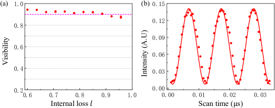
Figure 4: (a) The red dots are the values of $\mathrm{{V_{opt}}}$. The pink dashed line corresponds to a visibility of $90\%$. (b) The red dots are the interference fringes of the SALHI after optimization, corresponding to $G_{2}$$\approx$1.3 with $G_{1}$=3, $l$=0.96 ,and $\eta$=0.4, $\mathrm{{V_{opt}}=88\%}$.

6 Visibility restoration

Next, we provide an experimental demonstration of restoration of $\mathrm{{V_{SU}}}$ by optimizing $G_{2}$ in the SALHI. In practical applications such as radar or ranging measurement, when the parameters ($G_{1}$, $g_{1}$, $\eta$, $l$) are fixed, we can adjust only $G_{2}$ and $g_{2}$ to satisfy the optimization condition and improve the visibility. In the experiment, $W_{1}$ and $W_{2}$ are separated from the same laser as Fig. 1 (b) shown. Before the $W_{2}$ field enters the vapor cell, it passes through an attenuator and an AOM, which can be used to adjust the intensity and frequency of the $W_{2}$ field, respectively. Therefore, we can control $G_{2}$ by controlling the intensity and frequency of $W_{2}$, so that the optimal condition is satisfied to obtain the best visibility. The experimental data of the visibility after optimizing $G_{2}$ ($\mathrm{{V_{opt}}}$) are given in Fig. 4 (a) using red dots. $\mathrm{{V_{opt}}}$ is larger than the visibility without optimization ($\mathrm{{V_{SU}}}$), and at $l=0.6$, $\mathrm{V_{opt}}$ is 95%. As $l$ increases, $\mathrm{{V_{opt}}}$ can remain at $\sim 90\%$ (see the pink dashed line), and the optimized $G_{2}$ is small at the loss $l$ of 0.6-0.96 as in the theoretical prediction, such as $\mathrm{{V_{opt}}}$=88% with $G_{2}\approx 1.3$ when $l=0.96$, and Fig. 4 (b) shows the interference fringes of the SALHI after optimization. The results show that the visibility can be restored even at large internal loss by optimizing $G_{2}$, so the negative impact of internal loss on the properties of the SALHI can be mitigated. These experimental results are well consistent with the theoretical expectations.

7 Discussion and Conclusion

In conclusion, we have experimentally and theoretically researched the influence of the internal loss on the visibility of the SU(1, 1)-type ALHI. In general, the internal loss has a significant negative impact on the visibility. Moreover, we give the optimization condition $G_{1}G_{2}\sqrt{1-l}=g_{1}g_{2}\sqrt{1-\eta}$ for visibility restoration and experimentally demonstrate that the visibility can be restored to $\sim$90$\%$ over a large range of internal loss by optimizing the $G_{2}$ factor to satisfy the optimization condition. Finally, we also theoretically find that the optimization condition for $\mathrm{{SNR_{SU}}}$ enhancement is the same as that for visibility restoration. Visibility as a physical quantity that is easy to obtain and observe, which can be used as an experimental operational criterion to judge whether the $\mathrm{{SNR_{SU}}}$ is optimized. What we have found will guide significance for practical application of quantum measurement.

8 APPENDIX: Comparison of optimization conditions of ID and BHD

1. The optimization conditions of seed light field $\hat{a}_{s_{0}}$ input

After considering the losses $l$ and $\eta$, the optimal condition for the best $\rm{SNR_{SU}}$ under the ID is $G_{1}G_{2}\sqrt{1-l}=g_{1}g_{2}\sqrt{1-\eta}$, Obviously, this corresponds to the condition of the largest visibility. However, under the BHD, the quadrature component of interference output at phase dark point $\varphi=0$ is $\hat{X}_{\hat{a}_{s_{2}}}$,

$$\begin{split}\hat{X}_{\hat{a}_{s_{2}}}=&(G_{1}G_{2}\sqrt{1-l}+g_{1}g_{2}\sqrt{1-\eta})\hat{a}_{S_{0}}+G_{2}\sqrt{l}\hat{v}\\ +&(G_{2}g_{1}\sqrt{1-l}+G_{1}g_{2}\sqrt{1-\eta})\hat{S}_{a_{0}}^{\dagger}+g_{2}\sqrt{\eta}\hat{F}^{\dagger}\\ +&(G_{1}G_{2}\sqrt{1-l}+g_{1}g_{2}\sqrt{1-\eta})\hat{a}_{S_{0}}^{\dagger}+G_{2}\sqrt{l}\hat{v}^{\dagger}\\ +&(G_{2}g_{1}\sqrt{1-l}+G_{1}g_{2}\sqrt{1-\eta})\hat{S}_{a_{0}}+g_{2}\sqrt{\eta}\hat{F},\end{split}$$ (8)

therefore, under the BHD,

$$\begin{split}{\rm{SNR_{SU}}}=\dfrac{4(1-l)G^{2}_{1}G^{2}_{2}N_{\hat{a}_{s_{0}}}\delta^{2}}{\zeta^{2}_{1}+\zeta^{2}_{2}+\zeta^{2}_{3}},\end{split}$$ (9)

where $\zeta^{2}_{1}$=$(G_{1}G_{2}\sqrt{1-l}+g_{1}g_{2}\sqrt{1-\eta})^{2}$, $\zeta^{2}_{2}$=$(G_{2}g_{1}\sqrt{1-l}+G_{1}g_{2}\sqrt{1-\eta})^{2}$, $\zeta^{2}_{3}$=$G^{2}_{2}l+g^{2}_{2}\eta$. We also calculate the partial derivative to find the optimization condition, the result is,

$$\begin{split}2\sqrt{1-l}\sqrt{1-\eta}G_{1}G_{2}g_{1}g_{2}=2(1-\eta)g^{2}_{1}g^{2}_{2}+g^{2}_{2}+G^{2}_{2}.\end{split}$$ (10)

Obviously, this is different with the optimization condition of the largest visibility in Eq. (5).

2. The optimization conditions of initially prepared spin wave $\hat{S}_{a_{0}}$

From the Eq.(3), the visibility expression is:

$${\rm V_{SU}}\approx\dfrac{2G_{1}G_{2}g_{1}g_{2}\sqrt{1-l}\sqrt{1-\eta}}{G_{2}^{2}g_{1}^{2}(1-l)+G_{1}^{2}g_{2}^{2}(1-\eta)}.$$ (11)

Similarly, for largest visibility, the optimization condition is,

$$G_{2}g_{1}\sqrt{1-l}=G_{1}g_{2}\sqrt{1-\eta}.$$ (12)

Under the ID,

$${\rm SNR_{SU}}\approx\dfrac{4G_{1}^{2}G_{2}^{2}g_{1}^{2}g_{2}^{2}(1-l)(1-\eta)N_{\hat{a}_{s_{0}}}sin^{2}\varphi\delta^{2}}{B^{2}(A^{2}+B^{2}+C^{2})},$$ (13)

from the Eq.(7) we can get the optimization condition of best ${\rm SNR_{SU}}$ is $G_{2}g_{1}\sqrt{1-l}=G_{1}g_{2}\sqrt{1-\eta}$, which is also same as optimization of largest visibility in Eq. (12).

However, under the BHD,

$$\begin{split}{\rm{SNR_{SU}}}=\dfrac{4(1-l)G^{2}_{2}g^{2}_{1}N_{\hat{a}_{s_{0}}}\delta^{2}}{\zeta^{2}_{1}+\zeta^{2}_{2}+\zeta^{2}_{3}},\end{split}$$ (14)

the optimization condition of best ${\rm SNR_{SU}}$ is same as Eq. (10), which is also different with the optimization condition of largest visibility in Eq. (12).

In previous paper[14], we theoretically studied the ${\rm{SNR_{SU}}}$ using homodyne detection only considering optical loss $l$. In this paper, we further study the visibility and ${\rm{SNR_{SU}}}$ using ID and BHD with both losses $l$ and $\eta$ because these two losses are always exist simultaneously in practical application. We find that whether with optical input seed or initial atomic seed, the optimization condition for best ${\rm{SNR_{SU}}}$ using ID is same as that of largest visibility, but different with that using BHD.

Therefore, here we experimentally measure the signal using ID. We can intuitively judge whether the optimization conditions for best ${\rm{SNR_{SU}}}$ is achieved according to the visibility restoration. And furthermore, compared with BHD, the ID device is simpler and more suitable for practical application of the SALHI in radar and ranging measurements.

Funding This work was supported by the National Key Research and Development Program of China (2016YFA0302001); the National Natural Science Foundation of China (11874152, 11974111, 11654005, 91536114); the Shanghai Municipal Science and Technology Major Project (2019SHZDZX01); the innovation Program of Shanghai Municipal Education Commission (No. 202101070008E00099); the Fundamental Research Funds for the Central Universities; the Shanghai talent program and the Fellowship of China Postdoctoral Science Foundation (2020TQ0193).

Disclosures The authors declare no conflicts of interest.

Data Availability Data underlying the results presented in this paper are not publicly available at this time but may be obtained from the authors upon reasonable request.

References

- [1] X. Nie, J. Huang, Z. Li, W. Zheng, C. Lee, X. Peng, and J. Du, “Experimental demonstration of nonlinear quantum metrology with optimal quantum state,” \JournalTitleScience Bulletin 63, 469–476 (2018).
- [2] B. P. Abbott, R. Abbott, T. Abbott, F. Acernese, K. Ackley, C. Adams, T. Adams, P. Addesso, R. Adhikari, V. Adya et al., “Gw170817: observation of gravitational waves from a binary neutron star inspiral,” \JournalTitlePhysical Review Letters 119, 161101 (2017).
- [3] L. S. Collaboration, V. Collaboration, M. Collaboration, D. E. C. G.-E. Collaboration, D. Collaboration, D. Collaboration, L. C. O. Collaboration, V. Collaboration, M. Collaboration et al., “A gravitational-wave standard siren measurement of the hubble constant,” \JournalTitleNature 551, 85–88 (2017).
- [4] J. Liu, W. Liu, S. Li, D. Wei, H. Gao, and F. Li, “Enhancement of the angular rotation measurement sensitivity based on su (2) and su (1, 1) interferometers,” \JournalTitlePhotonics Research 5, 617–622 (2017).
- [5] M. Xiao, L.-A. Wu, and H. J. Kimble, “Precision measurement beyond the shot-noise limit,” \JournalTitlePhysical Review Letters 59, 278 (1987).
- [6] R. S. Bondurant and J. H. Shapiro, “Squeezed states in phase-sensing interferometers,” \JournalTitlePhysical Review D 30, 2548 (1984).
- [7] O. Steuernagel and S. Scheel, “Approaching the heisenberg limit with two-mode squeezed states,” \JournalTitleJournal of Optics B: Quantum and Semiclassical Optics 6, S66 (2004).
- [8] C. Gross, T. Zibold, E. Nicklas, J. Esteve, and M. K. Oberthaler, “Nonlinear atom interferometer surpasses classical precision limit,” \JournalTitleNature 464, 1165–1169 (2010).
- [9] Y.-J. Wang, D. Z. Anderson, V. M. Bright, E. A. Cornell, Q. Diot, T. Kishimoto, M. Prentiss, R. Saravanan, S. R. Segal, and S. Wu, “Atom michelson interferometer on a chip using a bose-einstein condensate,” \JournalTitlePhysical Review Letters 94, 090405 (2005).
- [10] M. Weitz, B. C. Young, and S. Chu, “Atomic interferometer based on adiabatic population transfer,” \JournalTitlePhysical Review Letters 73, 2563 (1994).
- [11] P. Hamilton, M. Jaffe, P. Haslinger, Q. Simmons, H. Müller, and J. Khoury, “Atom-interferometry constraints on dark energy,” \JournalTitleScience 349, 849–851 (2015).
- [12] B. Estey, C. Yu, H. Müller, P.-C. Kuan, and S.-Y. Lan, “High-resolution atom interferometers with suppressed diffraction phases,” \JournalTitlePhysical Review Letters 115, 083002 (2015).
- [13] M. Kasevich and S. Chu, “Measurement of the gravitational acceleration of an atom with a light-pulse atom interferometer,” \JournalTitleApplied Physics B 54, 321–332 (1992).
- [14] B. Chen, C. Qiu, S. Chen, J. Guo, L. Chen, Z. Ou, and W. Zhang, “Atom-light hybrid interferometer,” \JournalTitlePhysical Review Letters 115, 043602 (2015).
- [15] C. Qiu, S. Chen, L. Chen, B. Chen, J. Guo, Z. Ou, and W. Zhang, “Atom–light superposition oscillation and ramsey-like atom–light interferometer,” \JournalTitleOptica 3, 775–780 (2016).
- [16] A. Matsko, A. Savchenkov, V. Ilchenko, and L. Maleki, “Optical gyroscope with whispering gallery mode optical cavities,” \JournalTitleOptics Communications 233, 107–112 (2004).
- [17] P. A. Rosen, S. Hensley, I. R. Joughin, F. K. Li, S. N. Madsen, E. Rodriguez, and R. M. Goldstein, “Synthetic aperture radar interferometry,” \JournalTitleProceedings of the IEEE 88, 333–382 (2000).
- [18] T. Kubota, M. Nara, and T. Yoshino, “Interferometer for measuring displacement and distance,” \JournalTitleOptics letters 12, 310–312 (1987).
- [19] T. Gustavson, P. Bouyer, and M. Kasevich, “Precision rotation measurements with an atom interferometer gyroscope,” \JournalTitlePhysical Review Letters 78, 2046 (1997).
- [20] A. Peters, K. Y. Chung, and S. Chu, “High-precision gravity measurements using atom interferometry,” \JournalTitleMetrologia 38, 25 (2001).
- [21] P. Hamilton, M. Jaffe, J. M. Brown, L. Maisenbacher, B. Estey, and H. Müller, “Atom interferometry in an optical cavity,” \JournalTitlePhysical Review Letters 114, 100405 (2015).
- [22] X. Wu, Z. Pagel, B. S. Malek, T. H. Nguyen, F. Zi, D. S. Scheirer, and H. Müller, “Gravity surveys using a mobile atom interferometer,” \JournalTitleScience advances 5, eaax0800 (2019).
- [23] M.-K. Zhou, Z.-K. Hu, X.-C. Duan, B.-L. Sun, J.-B. Zhao, and J. Luo, “Precisely mapping the magnetic field gradient in vacuum with an atom interferometer,” \JournalTitlePhysical Review A 82, 061602 (2010).
- [24] C. F. Ockeloen, R. Schmied, M. F. Riedel, and P. Treutlein, “Quantum metrology with a scanning probe atom interferometer,” \JournalTitlePhysical Review Letters 111, 143001 (2013).
- [25] Y. Wu, J. Guo, X. Feng, L. Chen, C.-H. Yuan, and W. Zhang, “Atom-light hybrid quantum gyroscope,” \JournalTitlePhysical Review Applied 14, 064023 (2020).
- [26] S. Chen, L. Chen, Z.-Y. Ou, and W. Hang, “Quantum non-demolition measurement of photon number with atom-light interferometers,” \JournalTitleOptics express 25, 31827–31839 (2017).
- [27] F. Hudelist, J. Kong, C. Liu, J. Jing, Z. Ou, and W. Zhang, “Quantum metrology with parametric amplifier-based photon correlation interferometers,” \JournalTitleNature communications 5, 1–6 (2014).
- [28] J. Kong, J. Jing, H. Wang, F. Hudelist, C. Liu, and W. Zhang, “Experimental investigation of the visibility dependence in a nonlinear interferometer using parametric amplifiers,” \JournalTitleApplied Physics Letters 102, 011130 (2013).
- [29] M. I. Kolobov, E. Giese, S. Lemieux, R. Fickler, and R. W. Boyd, “Controlling induced coherence for quantum imaging,” \JournalTitleJournal of Optics 19, 054003 (2017).
- [30] Z. Ou, “Enhancement of the phase-measurement sensitivity beyond the standard quantum limit by a nonlinear interferometer,” \JournalTitlePhysical Review A 85, 023815 (2012).
- [31] M. Kacprowicz, R. Demkowicz-Dobrzański, W. Wasilewski, K. Banaszek, and I. Walmsley, “Experimental quantum-enhanced estimation of a lossy phase shift,” \JournalTitleNature Photonics 4, 357–360 (2010).
- [32] B. Yurke, S. L. McCall, and J. R. Klauder, “Su (2) and su (1, 1) interferometers,” \JournalTitlePhysical Review A 33, 4033 (1986).
- [33] K. Zheng, M. Mi, B. Wang, L. Xu, L. Hu, S. Liu, Y. Lou, J. Jing, and L. Zhang, “Quantum-enhanced stochastic phase estimation with the su (1, 1) interferometer,” \JournalTitlePhotonics Research 8, 1653–1661 (2020).
- [34] Y. Liu, J. Li, L. Cui, N. Huo, S. M. Assad, X. Li, and Z. Ou, “Loss-tolerant quantum dense metrology with su (1, 1) interferometer,” \JournalTitleOptics Express 26, 27705–27715 (2018).
- [35] A. M. Marino, N. C. Trejo, and P. D. Lett, “Effect of losses on the performance of an su (1, 1) interferometer,” \JournalTitlePhysical Review A 86, 023844 (2012).
- [36] M. Manceau, G. Leuchs, F. Khalili, and M. Chekhova, “Detection loss tolerant supersensitive phase measurement with an su (1, 1) interferometer,” \JournalTitlePhysical Review Letters 119, 223604 (2017).
- [37] E. Giese, S. Lemieux, M. Manceau, R. Fickler, and R. W. Boyd, “Phase sensitivity of gain-unbalanced nonlinear interferometers,” \JournalTitlePhysical Review A 96, 053863 (2017).
- [38] M. Manceau, F. Khalili, and M. Chekhova, “Improving the phase super-sensitivity of squeezing-assisted interferometers by squeeze factor unbalancing,” \JournalTitleNew Journal of Physics 19, 013014 (2017).
- [39] J. Xin, H. Wang, and J. Jing, “The effect of losses on the quantum-noise cancellation in the su (1, 1) interferometer,” \JournalTitleApplied Physics Letters 109, 051107 (2016).
- [40] W. Du, J. Chen, Z. Ou, and W. Zhang, “Quantum dense metrology by an su (2)-in-su (1, 1) nested interferometer,” \JournalTitleApplied Physics Letters 117, 024003 (2020).
- [41] D. Li, B. T. Gard, Y. Gao, C.-H. Yuan, W. Zhang, H. Lee, and J. P. Dowling, “Phase sensitivity at the heisenberg limit in an su (1, 1) interferometer via parity detection,” \JournalTitlePhysical Review A 94, 063840 (2016).
- [42] Y. Michael, I. Jonas, L. Bello, M.-E. Meller, E. Cohen, M. Rosenbluh, and A. Pe’er, “Augmenting the sensing performance of entangled photon pairs through asymmetry,” \JournalTitlePhys. Rev. Lett. 127, 173603 (2021).
- [43] K. Hammerer, A. S. Sørensen, and E. S. Polzik, “Quantum interface between light and atomic ensembles,” \JournalTitleReviews of Modern Physics 82, 1041 (2010).
- [44] B. E. Anderson, P. Gupta, B. L. Schmittberger, T. Horrom, C. Hermann-Avigliano, K. M. Jones, and P. D. Lett, “Phase sensing beyond the standard quantum limit with a variation on the su (1, 1) interferometer,” \JournalTitleOptica 4, 752–756 (2017).
- [45] Z.-D. Chen, C.-H. Yuan, H.-M. Ma, D. Li, L. Chen, Z. Ou, and W. Zhang, “Effects of losses in the atom-light hybrid su(1, 1) interferometer,” \JournalTitleOptics Express 24, 17766–17778 (2016).
- [46] R. Demkowicz-Dobrzanski, U. Dorner, B. Smith, J. Lundeen, W. Wasilewski, K. Banaszek, and I. Walmsley, “Quantum phase estimation with lossy interferometers,” \JournalTitlePhysical Review A 80, 013825 (2009).
- [47] U. Dorner, R. Demkowicz-Dobrzanski, B. Smith, J. Lundeen, W. Wasilewski, K. Banaszek, and I. Walmsley, “Optimal quantum phase estimation,” \JournalTitlePhysical Review Letters 102, 040403 (2009).