Tackling Multipath and Biased Training Data for
IMU-Assisted BLE Proximity Detection

Abstract

Proximity detection is to determine whether an IoT receiver is within a certain distance from a signal transmitter. Due to its low cost and high popularity, Bluetooth low energy (BLE) has been used to detect proximity based on the received signal strength indicator (RSSI). To address the fact that RSSI can be markedly influenced by device carriage states, previous works have incorporated RSSI with inertial measurement unit (IMU) using deep learning. However, they have not sufficiently accounted for the impact of multipath. Furthermore, due to the special setup, the IMU data collected in the training process may be biased, which hampers the system’s robustness and generalizability. This issue has not been studied before.

We propose PRID, an IMU-assisted BLE proximity detection approach robust against RSSI fluctuation and IMU data bias. PRID histogramizes RSSI to extract multipath features and uses carriage state regularization to mitigate overfitting due to IMU data bias. We further propose PRID-lite based on a binarized neural network to substantially cut memory requirements for resource-constrained devices. We have conducted extensive experiments under different multipath environments, data bias levels, and a crowdsourced dataset. Our results show that PRID significantly reduces false detection cases compared with the existing arts (by over 50%). PRID-lite further reduces over 90% PRID model size and extends 60% battery life, with a minor compromise in accuracy (7%).

I Introduction

Proximity detection is to decide whether an IoT receiver is within a certain distance, say 5 meters, from a signal transmitter. If so it is a “proximity” event, or “no proxmity” event otherwise. Free from human operation, such decision enables many proximity-based services (PBS), such as contact tracing [1, 2, 3, 4], proximity marketing [5], and presence or check-in/checkout logging [6, 7]. These services often need to detect proximity independent of receiver carriage state, i.e., independent of whether the receiver is held in swinging hands, read positions, a pocket, backpack, side bag, and so on.

Many signals have been studied for proximity detection, such as radio frequency (RF) [8, 9], ultrasound [10], and LiDAR [11]. Among them, Bluetooth Low Energy (BLE) emerges as the most promising due to its low cost, low power consumption, appropriate coverage range (around 10 meters), and wide availability in IoT devices. In this work, we consider a common BLE-based PBS deployment scenario where no hard partition (or wall) cuts between the receiver and the transmitter at the time of proximity detection. (Detecting partition between two devices is an independent issue outside the scope of this study. Interested readers may refer to [12, 13] and references therein.)

Traditionally, proximity is detected by measuring the received signal strength indicator (RSSI) and correlating it with distance, with the intuition that a lower RSSI means larger distance, and vice versa. However, RSSI may be severely affected by environment and receiver carriage state, leading to signal fading, fluctuation, and attenuation. To address that, much of the existing work employs deep learning to find a high-dimensional classification boundary from the RSSI values (see, for example, [14, 15]). However, these models are often not robust against RSSI fluctuation because the received signals may be randomly affected by nearby mobile objects (e.g., pedestrians, vehicles, rotating fans, etc.). As a result, the decision may be noisy, leading to less than satisfactory results.

To account for the impact of carriage state on RSSI, inertial measurement unit (IMU) readings are often collected as training data [14]. Unfortunately, such a collection process does not always faithfully reflect the operating condition in reality (i.e., independence of carriage state in the general case). In other words, the training data may be biased, i.e., the dataset does not guarantee the carriage state, as given by IMU readings, to be independent of proximity. If such a bias is not accounted for properly, deep learning models could correlate the IMU readings to proximity, leading to overfitting and generalization issues, and performance highly dependent on the data acquisition process.

To tackle the above multipath and biased training data issues, we propose PRID, a novel, accurate, and generalizable IMU-assisted BLE proximity detection which is robust against RSSI fluctuation and IMU data bias. We overview PRID in Figure 1. In the forward (online) path, PRID, using a sliding window (a few seconds), encodes BLE RSSIs and IMU data as feature vectors using RSSI histogramization and carriage feature encoding modules, respectively (signal encoding step). After concatenating the feature vectors, a trained binary classifier based on deep neural network (DNN) is employed to detect proximity (proximity classification step). In the backward  path for offline training, PRID employs carriage state regularization to reduce the IMU overfitting problem of the classifier.

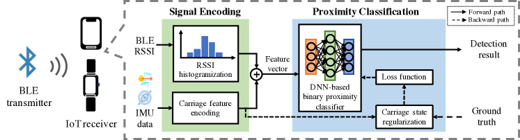
Figure 1: System overview of PRID.

The major contributions of this work are as follows:

• RSSI histogramization to mitigate multipath impact: Multipath leads to a spread in RSSI distribution, which sheds lights on the features in the environment. Therefore, to mitigate RSSI fluctuations due to multipath, we propose to represent the RSSI time series within a sliding window as a histogram. Through such a “histogramization” process, the multipath environment is modeled as a distribution for training and inference purposes.

• Carriage state regularization for potentially biased training data: We study, for the first time, how to mitigate IMU training data bias for BLE proximity detection. We propose carriage state regularization, which first employs importance sampling to reduce the discrepancy between the IMU features of the “proximity” state and that of the “no proximity” state in the training data. Then, it applies the resultant sampling weights to a loss function in the training step, thereof effectively reducing IMU overfitting in the DNN-based proximity classifier.

• PRID-lite: Achieving memory efficiency for resource-constrained IoT devices: While PRID is efficient and deployable on smartphones commonly available on the market nowadays, its memory requirement may still be demanding for some low-end IoT devices with extremely constrained resources, such as contact tracing tokens [3], smart car keys [7], and audio guide devices for museums [16]. To further extend its use to resource-constrained IoT devices, we propose PRID-lite, a lightweight variant of PRID achieving high memory efficiency with little cost in performance. We employ model binarization on the DNN-based proximity classifier to achieve a proper trade-off between neuron quantity and neuron precision. Moreover, due to the memory-efficient bit-wise operation between binarized neurons, PRID-lite is more energy-conserving than floating-point manipulation and computationally efficient.

PRID and PRID-lite are easily implementable and deployable. We have developed them on commercial smartphones and IoT devices (Android smartwatch, Raspberry Pi Zero, and ESP-32). To validate our design, we conduct extensive experiments on multiple sites with different multipath environments and levels of IMU data bias, including the TC4TL challenge dataset [17], which is a crowdsourced public dataset for automated contact tracing. Our results show that PRID achieves substantial improvement as compared with the state-of-the-arts (with more than 50% reduction in false detection cases in our dataset). PRID-lite reduces the model size of PRID by 94% (from 5MB to 0.3MB) and extends battery life by more than 60% in our implementations, with only a minor compromise in accuracy (7% reduction in F-score). This demonstrates that PRID-lite is deployable in most resource-constrained devices.

The remainder of this paper is organized as follows. We discuss related work in Section II, and how PRID encodes RSSI and IMU signals in Section III. In Section IV, we present PRID’s online proximity classification and its offline training with carriage state regularization. In Section V, we detail PRID-lite. Later, we cover illustrative experimental results in Section VI and conclude in Section VII.

II Related Work

Distance, multipath environment, and carriage state are three major factors that affect RSSI and hence proximity detection. In the following, we discuss previous works on these three factors.

Most of the early works on BLE proximity detection only consider the relationship between RSSI and distance. By assuming BLE signal merely attenuates over distance, they investigate how RSSI decreases as distance goes up by regression approaches – it is intuitive to determine proximity events by ranging from RSSI. The most common regression model is the log-distance path loss model [18], which builds the exponential relationship between RSSI and distance. Some of its variants can be found in [19]. Linear and inverse proportion relations are also studied in [20]. However, since these works fail to consider the multipath environment and carriage state, such regression approaches are mostly unreliable in practice.

Many recent works have considered the RSSI distortion caused by the multipath environments. Their approaches are either based on noise reduction or sequential correlation upon an RSSI sliding window. The noise reduction works consider the RSSI distortion as signal noise and study various signal filters against multipath environments. Works in [20, 21, 22, 15] leverage statistical features (such as mean and median) for noise reduction. Other works in [23, 24, 25, 26] apply Bayesian filters to process RSSI. Although these works improve detection accuracy in the settings under study, they suffer from poor extensibility to different environments since they assume the identical noise distribution over different environments. Besides, some research works explore RSSI sequential correlation to detect proximity. Research work in [27] models RSSI sequence as a Markov chain and denotes the proximity as its model’s binary state. The work of [14] experiments with several deep learning models on RSSI time series, trying to find a high dimensional classification boundary. However, since multipath fading is complex and unpredictable, the resultant RSSI fluctuations are rather random and noisy. Such fluctuation adversely affects these models, and, as a result, they cannot learn a good classification boundary. In comparison, PRID does not assume any noise distribution or sequential correlation. Since the multipath effect leads to a spread in RSSI distribution, it represents the RSSI time series as a histogram and takes advantage of such signal fluctuation to extract environmental features.

Since different carriage states could render RSSI completely different even under the same environment and distance, some works further account for carriage state on BLE proximity detection. The approach in [4] categorizes carriage state as a known set of several on-body positions (such as being handheld or placed in a pocket). They adjust their RSSI-based proximity threshold by carriage state while detecting proximity. However, this scheme relies heavily on manual labeling and works only for pre-defined states, making it hard to deploy or generalize in practice. To efficiently reflect carriage state, the work in [14] introduces IMU and leverages deep learning to model the impact of carriage states on RSSI values. To improve model generalizability, they crowdsource data from volunteers. However, their models cannot generalize well since they have not considered the bias in the IMU training data. As a comparison, PRID uses IMU to reflect carriage state and addresses the bias issue by applying carriage state regularization. By accounting for the correlation between IMU readings and proximity states in training data, the regularization greatly reduces the IMU overfitting problem.

III Signal Encoding in PRID

We present in this section how PRID processes RSSI and IMU signals so as to encode the system inputs to feature vectors. In Section III-A, we discuss histogramization for BLE RSSI. In Section III-B, we introduce carriage feature encoding based on IMU readings.

III-A RSSI Histogramization

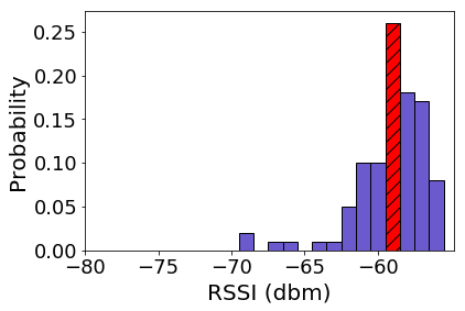
(a) Without pedestrian.

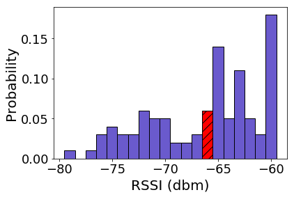
(b) With pedestrians.

Figure 2: BLE RSSI histogram under environments w/o pedestrians roaming around. The shaded red bin represents the median RSSI values.

Although an individual RSSI measurement is noisy, the distribution of RSSIs over time tends to be informative in representing environmental features. Based on this observation, we use histogram to represent the distribution of RSSI fluctuation so as to capture RSSI distortion as well as the multipath in the environment. In the histogram, we present RSSI over a time period into various buckets, with each bucket denoting the appearance frequency of a certain RSSI range. Specifically, histogramization converts a series of RSSIs into a vector

$$R=\left[r_{1},r_{2},...,r_{n}\right],$$ (1)

where $r_{i}$ denotes the normalized number of RSSI (over a sliding window) that belongs to the $i^{th}$ bucket. We set each bucket to cover the same range length (bin size)

$$\delta=\frac{\phi_{max}-\phi_{min}}{n},$$ (2)

where $\phi_{max}$ and $\phi_{min}$ represent RSSI extrema (maximum and minimum) that we consider, where, in our case, they are separately set to be $0\ dBm$ and $-100\ dBm$.

Figure 2 shows an example that illustrates the capability of RSSI histogram in representing RSSI distortions and multipath environment. In the example, we collect RSSI in a corridor where the signal receiver is 3 meters from a transmitter, and the collection lasts for 10 seconds (around 90 RSSI values are received). Figure 2a is collected at night when no pedestrian passes; and Figure 2b is collected on a busy afternoon with people walking around. Due to the multipath environments causing RSSI distortions to different extents, RSSI median value (denoted as the red shaded bin) shifts between two figures without distance change, which violates the assumption that a lower RSSI means a larger distance and fails its derivative methods. Nonetheless, RSSI histogramization represents the RSSI time series as a signal fluctuation distribution that could account for such influences from multipath environments. For one thing, from static to dynamic environments, as the more complex multipath effect (as in the Figure 2b case) renders a larger RSSI distortion (where RSSIs are sequentially noisy), it also causes a larger signal fluctuation that leads to a spread in RSSI distribution. For another, the fluctuation enlarges the inconsistency between histogram buckets so that its shape tends to be disordered. Besides the implication of RSSI distortion and the multipath, the histogram also contains distance information because the buckets are gathered by the RSSI range.

In our findings, this observation is also applicable to many non-line of sight and even cross-site scenarios. This is because a complex environment is likewise to cause a complex fading effect, rendering a severe RSSI distortion with a large signal fluctuation. This shows that the RSSI histogram is a powerful feature that is capable of representing multipath environments.

III-B Carriage Feature Encoding

We extract several features from IMU measurements to reflect carriage states. Generally, IMU includes three categories of signals: gravity, linear acceleration, and angular velocity. Gravity can be naturally used to infer device attitude. Linear acceleration and angular velocity, on the other hand, reflect the movement of a device. We argue that the device movement is also an important factor in reflecting carriage states. This is because these signals can further differentiate carriage states when devices have similar attitudes. For instance, the angular velocity along phone azimuth is much larger than its pitch when its user walks around with a phone in the front trouser pocket, while this situation reverses if the phone is in back pocket; in reality, such two carriage states could have different impacts on RSSI due to their different on-body positions.

We extract carriage features from a period of IMU data (of a few seconds). Formally, we denote the feature vector by

$$C=\left[c_{1},c_{2},...,c_{m}\right].$$ (3)

For gravity, we directly average the values along its three dimensions – the gravity projections of a device’s 3D coordinates – to reflect device attitude over time. For linear acceleration and angular velocity, we encode them by extracting some statistical features: energy, variance, skewness, kurtosis, and entropy. Since feature extraction on IMU data is not the focus of this work, we empirically employ these features to reflect carriage states and summarize them in Table I.

TABLE I: Carriage feature elements extracted from IMU data.

[t] Feature Formula Source^∗ Mean $\frac{1}{N}\sum_{i=1}^{N}x_{i}$ G Energy $\frac{1}{N}\sum_{i=1}^{N}{x_{i}}^{2}$ L, A Variance $\frac{1}{N}\sum_{i=1}^{N}(x_{i}-\bar{x})^{2}$ L, A Skewness $E[(\frac{x-\bar{x}}{\sigma})^{3}]$ L, A Kurtosis $E[(\frac{x-\bar{x}}{\sigma})^{4}]$ L, A Entropy $E[I(x)],$ L, A where $I(x)=-\ln\left[Pr\left(\frac{x-\min(x)}{\max(x)-\min(x)}\right)\right]$ * G: gravity, L:linear acceleration, A: angular velocity

IV Proximity Classification in PRID

We discuss in this section how PRID detects proximity given the feature vectors of RSSIs and carriage states. In Section IV-A, we present the design of the DNN-based proximity classifier. In Section IV-B, we discuss carriage state regularization for training the classifier.

IV-A DNN-based Binary Proximity Classifier

As mentioned, RSSI histogram $R$ provides environment and distance features, while carriage feature vector $C$ reflects carriage state. We need a classification model that jointly considers these inputs to estimate

$$y=Pr\left(Y=1|R,C\right),$$ (4)

where $y$ is the classifier output regarding the proximity state $Y$. As mentioned, proximity state is either ”proximity” event (1) or ”no proximity” event (0), i.e.,

$$Y=\begin{dcases}1,&\text{if }D\leq\tau\,;\\ 0,&\text{otherwise}\,,\\ \end{dcases}$$ (5)

where $\tau$ is the pre-defined proximity threshold and $D$ is the physical distance.

Unfortunately, it is intractable to handcraft such a model with those high-dimensional inputs. Therefore, we leverage deep learning to extract features from those inputs and correlate them with the proximity state. Specifically, the RSSI histogram and the carriage features, which are encoded over the same period, are concatenated as a feature vector. We then use a deep neural network (DNN)-based proximity classifier to determine proximity states from the feature vectors.

We illustrate the classifier structure in Figure 3. It consists of an input layer (omitted in the figure), an output layer, and several hidden layers. Each hidden layer is comprised of network neurons, a normalization method, and an activation function. We employ batch normalization (BN) [28] as the normalization method and Mish [29] as the activation function. As a convention, Softmax serves as the classifier’s output layer. As for the model training, we choose cross-entropy as the loss function and train the network with the Adam optimizer. We have also tried other common deep learning model tricks, such as using ReLU as the activation function; they show a similar performance in this task. Readers interested in such tricks may refer to [30, 31, 32] and the references therein.

Figure 3: The network structure of the proximity classifier in PRID.

IV-B Carriage State Regularization

We illustrate in Figure 4 the problem of BLE proximity detection by posing it as a graph model. Each node represents a factor or an event in the BLE proximity detection system. In the figure, the considerations – carriage state, distance, and multipath environment – are three major factors that influence RSSI; proximity state is the comparison result between proximity threshold (omitted in the graph for simplicity) and physical distance. We denote RSSI with all of its representation as $R$ and IMU reading with its derived carriage state features as $C$. Take PRID as an example, we denote $R$ as an RSSI histogram and $C$ as carriage feature vector.

In the figure, a directed edge describes causality between nodes. Specifically, a directed edge pointing A to B indicates that a variation in A could lead to a status change in B, being other factors unchanged. For example, an edge pointing from distance to RSSI means: without other factors changing, a larger distance would lead to a smaller RSSI value. Note that, the association absence between any two nodes assumes their prior independence; for instance, carriage state and distance are independent being RSSI unknown, but they are correlated when the RSSI is given (according to d-separation [33]).

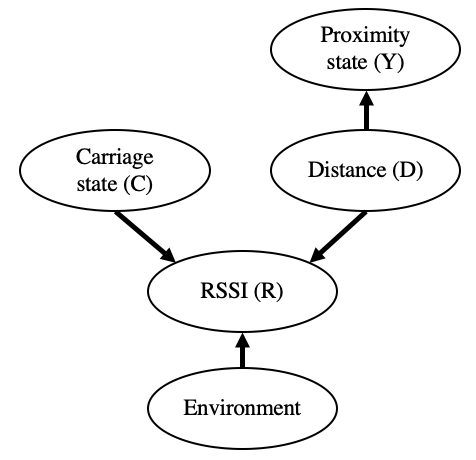
Figure 4: Graphical model of BLE proximity detection. Each node denotes a factor or event in proximity detection. A directed edge denotes causality between its connected nodes.

Essentially, the BLE proximity detection task is to model those causalities beforehand, so that we can use the established model to estimate the proximity state from those observable inputs. For regression works that only consider distance and RSSI, they model $Pr(R|D)$ because distance causes RSSI change. In practice, they estimate the distance from the observable RSSI

$$Pr(D|R)\propto Pr(R|D),$$ (6)

assuming $Pr(D)$ is uniformly distributed. Then, proximity state can be estimated the same way as in Equation 5, with the goal of modeling the causality from distance to proximity state in Figure 4. Apparently, these works suffer inaccuracy in practice due to the absence of carriage state and environment as well as their related edges. Thus, later works further consider environment and carriage state, aiming to model $Pr(R|C,Y)$ in the training phase. Since $Pr(R|C,Y)$ is intractable, they leverage deep learning to directly learn $Pr(Y|R,C)$ from data, assuming that

$$Pr(Y|C,R)\propto Pr(R|Y,C).$$ (7)

However, Equation 7 is valid only if proximity state $Y$ and carriage state $C$ are independent because

$$Pr(Y|C,R)=\frac{Pr(Y,C,R)}{Pr(C,R)}\propto Pr(R|Y,C)Pr(Y|C).$$ (8)

For using non-parametric models as deep learning ones, we expect this independence in training data to guarantee the established model to make unbiased estimations in practice. In other words, instead of determining proximity from carriage state, we want the model to detect proximity based on RSSI representations while considering carriage state impact on RSSI. Unfortunately, it is usually tricky to guarantee such unbiased training data in quantity – for one thing, IMU is highly sensitive to user activities, which varies in different scenarios. For another, acquiring such data is labor-intensive, systems from the literature (such as the work in [17]) crowdsource data from volunteers for better adaptability in different environments; this uncontrolled data acquisition process makes it harder to guarantee an unbiased training dataset. As a result, the built model $Pr(Y|C,R)$ suffers bias from $Pr(R|Y,C)$, and its performance is highly manipulated by training data. We refer to this issue as an IMU overfitting problem because the learned model falsely correlates IMU with proximity state when this discrepancy from independence appears in the training data. Apparently, this issue hinders the models from generalizing well.

To tackle this IMU overfitting problem, we propose carriage state regularization to supervise the training process of the DNN-based proximity classifier. Intuitively, carriage state regularization aims to cut off the correlation between the carriage feature and proximity state from the training data, so as to force the proximity classifier to learn the carriage state’s impact on RSSI.

Carriage state regularization leverages importance sampling to account for the distribution discrepancy of the carriage feature with different proximity states. We divide the training dataset $D$ into two groups $S=S_{Y=0}\cup S_{Y=1}$, according to their proximity state $Y$. The discrepancy is caused by the fact that these two groups are drawn from different distributions so that $Pr(C|Y=1)\neq Pr(C|Y=0)$. Such a discrepancy can be reduced by reweighting one group to match the other. Thus, with the goal to tackle the resultant overfitting problem, we reweight the training loss to reduce the discrepancy by

$$L^{\prime}(y_{i},Y_{i})=\frac{Pr(C_{i}|Y=1)}{Pr(C_{i}|Y=0)}L(y_{i},Y_{i})=w_{i}L(y_{i},Y_{i}),$$ (9)

where $L(\cdot)$ calculates training loss from detection result $y_{i}$ and proximity state $Y_{i}$, and $w_{i}$ represents the sampling weight.

Let $\boldsymbol{w}^{+}$ be the set of weights corresponding to the positive samples, i.e., $\boldsymbol{w}^{+}=\left\{w_{i}|s_{i}\in S_{Y=1}\right\}$. Similarly, the weight set for negative ones are $\boldsymbol{w}^{-}=\left\{w_{i}|s_{i}\in S_{Y=0}\right\}$. In this work, we aim to reweight $S_{Y=1}$ to match $S_{Y=0}$. We thus set all $w_{i}\in\boldsymbol{w}^{-}$ to be 1 and calculate $\boldsymbol{w}^{+}$. We use the kernel method to bridge the distribution discrepancy in the feature space (kernel mean matching [34]), that is

$$\min_{\boldsymbol{w^{+}}}\quad\frac{1}{2}(\boldsymbol{w^{+}})^{T}K\boldsymbol{w^{+}}-\kappa^{T}\boldsymbol{w^{+}}$$ (10)

$$\begin{array}[]{r@{\quad}l@{}l@{\quad}l}s.t.&\sum_{i=1}^{||\boldsymbol{w^{+}}||}w^{+}_{i}=||\boldsymbol{w^{+}}||\\ &0\leq w^{+}_{i}\leq w_{max},\ i=1,2,3\ldots,||\boldsymbol{w^{+}}||\end{array},$$ (13)

where we set $w_{max}$ as 10. The kernel computations are

$$K_{ij} :=k(C^{+}_{i},C^{+}_{j}),$$ (14)

$$\kappa_{i} :=\frac{||\boldsymbol{w^{+}}||}{||\boldsymbol{w^{-}}||}\sum_{j=1}^{||w^{-}||}k(C^{+}_{i},C^{-}_{j}),$$ (15)

where $k(\cdot,\cdot)$ is the radial basis function (RBF) kernel (the kernel width $\gamma=1.0$); we solve this quadratic program problem by the interior point method [35].

Note that carriage state regularization is general for IMU-assisted BLE proximity detection. Although we explain this regularization on the carriage feature, it is also applicable to other features that reflect carriage states.

V PRID-lite: Achieving Memory Efficiency

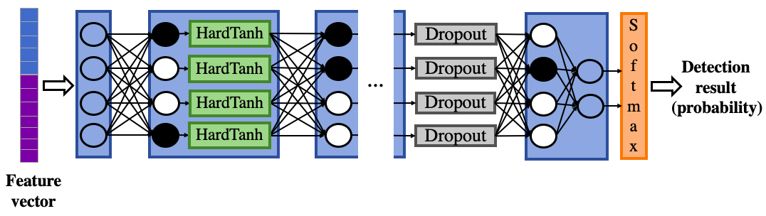
Figure 5: The network structure of proximity classifier in PRID-lite.

In PRID, most of the storage burden comes from the DNN-based proximity classifier. Normally, we use the larger neural network (with more neurons) for better generalization. However, a larger neural network not only requires more memory but also increased energy consumption that some resource-constraint devices cannot afford. Thus, the constrained resource limits us from using a large neural network, which hinders the proximity classifier from being accurate.

Since a neural network’s nature is to encode training data into its neuron connections, the neural network needs to be large enough to perform well; thus, we apply binarized neurons to build a larger network when the model size is constrained. Instead of using a floating-point number, a binarized neuron weight is either 1 or -1 (represented by a bit). This allows us to replace a full-precision neuron to be 32 binarized neurons, which enlarges the model structure in terms of neuron quantity. In addition, this binarization replaces the floating-point multiplication between neurons by bit-wise operation, which is faster and lighter for IoT devices to process. Although this binarization causes information loss between neurons – which inevitably renders inaccuracy of binarized neural network in comparison to its full-precision counterpart with enough neuron quantity – it is likely to gain a better performance by compromising the neuron precision for a larger network structure when device resources limit the scaling up of the model.

We illustrate the binarized proximity classifier structure in Figure 5. Compared with the proximity classifier from PRID, we binarize parts of its neurons (colored in white and black) and apply the activation function HardTanh to the hidden layers. We maintain the neuron precision of the input and last hidden layer because they are important in conveying information; but this would not cause severe memory burdens since these two layers are usually much smaller than the other layers. For general regularization, we add one dropout layer between the last two hidden layers. We train the network by using the same tricks as in the proximity classifier in PRID, except that we employ “straight-through estimator” [36] to tackle the binarized neuron training problem.

VI Illustrative Experimental Results

In this section, we show the illustrative experimental results of PRID and PRID-lite. We first discuss the experimental settings in Section VI-A, followed by the illustrative results in Section VI-B.

VI-A Experimental Settings

We have implemented PRID and PRID-lite and conducted extensive experiments to validate their performance. We run PRID on an Android smartphone, which continuously scans any surrounding BLE signals and logs the IMU data. For PRID-lite, we deploy our implementation on multiple resource-constrained IoT devices, including an Android smartwatch, a single-board computer Raspberry Pi Zero (Pi Zero), and a microcontroller unit ESP-32. Detailed specifications of the IoT devices are listed in Table III.

In our implementation of the DNN-based binary proximity classifier, we employ three fully connected layers with 700, 900, and 700 hidden nodes. Unless specified, it is for both PRID and PRID-lite.

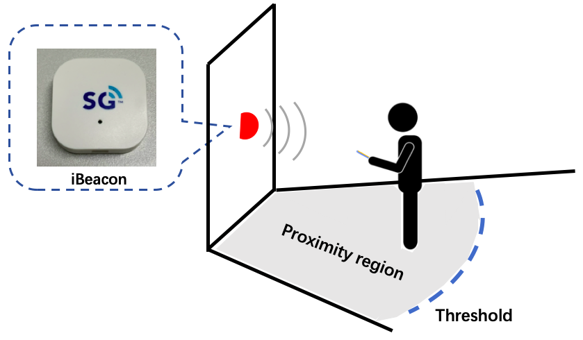
Figure 6: Illustration of data collection. The dotted line stands for proximity threshold. The user either moves within the proximity region or outside the proximity threshold.

We verify the system performance through an experiment on fields and an evaluation on a public crowdsourced dataset [17]. In our experiment, we set up a commercial iBeacon as the BLE transmitter. The iBeacon is attached to a wall 1.2 meters above the ground (as illustrated in Figure 6). It advertises 10 BLE handshaking messages per second with reference TX power (RSSI measured at 1 meter) of -59dBm. We invite multiple users for data collection. They carry smartphones either by hands or in pockets (decided by the users) and can move within 12m of the transmitter. We collect data in three venues: a crowded indoor junction (dynamic environment), an indoor open space with a few pedestrians (semi-dynamic environment), and a quiet outdoor region (static environment). In total, we collect RSSI readings for around 5 hours for model training and another one hour for performance testing. The detailed collecting hour of training data is shown in Table II. To fairly reflect reality, the carriage state and proximity state labels are carefully decoupled in the test data. In addition, we repeat the experiments for the proximity thresholds of 6m and 2m, corresponding to different proximity requirements in typical PBS applications (such as proximity marketing) and contact tracing scenarios, respectively.

We also validate our scheme on a public dataset from TC4TL challenge [17], a BLE proximity detection competition for automated contact tracing. The TC4TL dataset contains more than 25,000 crowdsourced RSSI sequences with each sequence ranging from 10 to 150 seconds. It covers several common environments and carriage states for contact tracing and restricts users to move within 4.5m from transmitters. We use the 2m proximity threshold in the evaluation since it is a common safe distance for contact tracing.

For a better evaluation, we separately train and test all the methods (including comparison schemes and our method) on the two datasets. We chunk the test data into time periods of 5s as well as the sliding window length. The evaluation metrics of this experiment are shown as follows:

• Accuracy: Accuracy is a common and intuitive metric for evaluating classifier quality. It denotes the proximity state as $Y$ and detection result as $Det$. The system precision and recall is calculated as

  $$Precision=\frac{||\{Y=1\}\cap\{Det=1\}||}{||\{Det=1\}||},$$ (16)

  $$Recall=\frac{||\{Y=1\}\cap\{Det=1\}||}{||\{Y=1\}||}.$$

  F-score is their harmonic mean, which is computed by

  $$F_{1}=\frac{2\times Precision\times Recall}{Precision+Recall}.$$ (17)

• False detection rate: Accuracy mainly focuses on system discernment on positive events, while recognizing proximity events and reducing false alarms are both essential in many PBS applications (such as contact tracing); thus, we further use a false detection rate to compare system performance. We follow the metric in [14] and employ nDCF to measure the false detection rate. We evaluate the detection error as the probability of missing contact (proximity) event $E_{miss}$ and false alarm $E_{fa}$, which are computed by

  $$E_{miss} = \frac{||\{Y=1\}\cap\{Det=0\}||}{||\{Y=1\}||},$$ (18)

  $$E_{fa} = \frac{||\{Y=0\}\cap\{Det=1\}||}{||\{Y=0\}||}.$$

  The evaluation nDCF is their normalized decision cost function

  $$nDCF=\frac{w_{miss}E_{miss}+w_{fa}E_{fa}}{\min(w_{miss},w_{fa})},$$ (19)

  where we use weights $w_{miss}=1$ and $w_{fa}=1$ in this experiment.

We compare our scheme with the following state-of-the-art schemes:

• Temporal 1-D convolutional network (Conv1D) [14]: Conv1D is a deep learning-based binary regressor. It uses raw RSSI and IMU data over a time period as input. In the experiments, we use one convolutional (with kernel size of $1\times 5$) and three fully-connected layers. Its neuron quantity is set to be similar to that of PRID.

• ProxiTrak [15]: ProxiTrak employs a random forest to detect proximity events. It extracts mean, minimum, maximum, and standard deviation from both the RSSI sliding window and inter-packet duration (IPD). It further conducts majority voting on the detection results to mitigate random noise. In our experiments, we follow the original paper to set the sliding window’s length to be 2s, and then aggregate results in 5s.

• Log-distance path loss model (LDPL) [20]: LDPL is a classic distance estimation technique and wildly used in commercial regression-based proximity detection systems. The distance is estimated by

  $$distance=10^{\frac{TX-RSSI}{10n}},$$ (20)

  where $n$ is a fading parameter learned from training data and TX denotes the reference RSSI measured at 1m. It detects proximity events by comparing the resultant distance with the proximity threshold. To alleviate signal fluctuation, we calculate RSSI by the mean value over a sliding window of 5s.

VI-B Illustrative Results

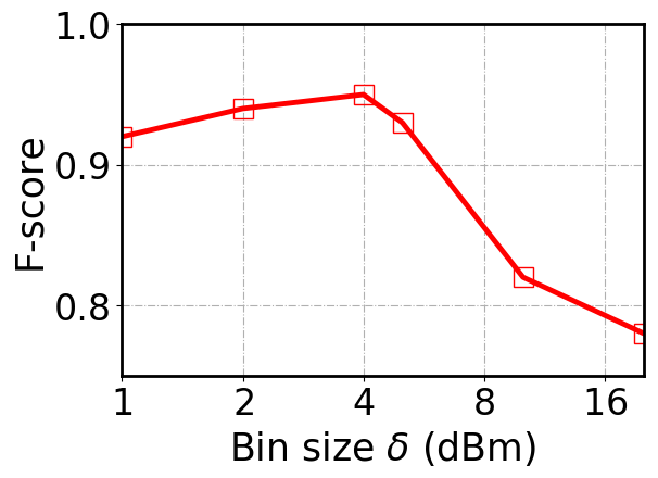
Figure 7: RSSI histogram bin size setting.

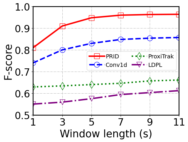
Figure 8: F-score against sliding window length.

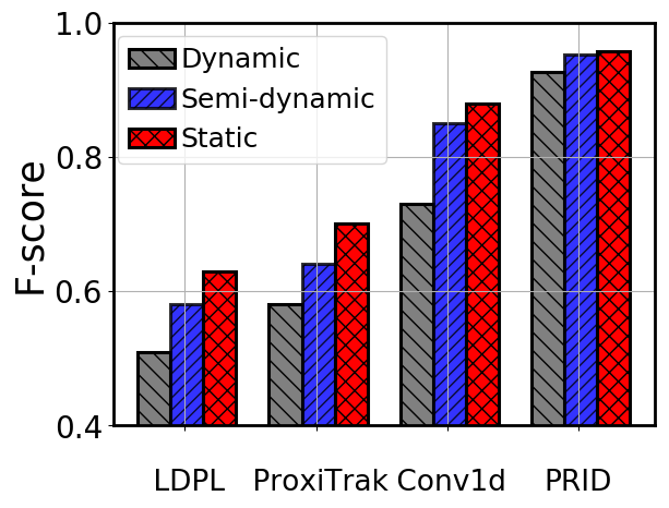
Figure 9: F-score under different sites.

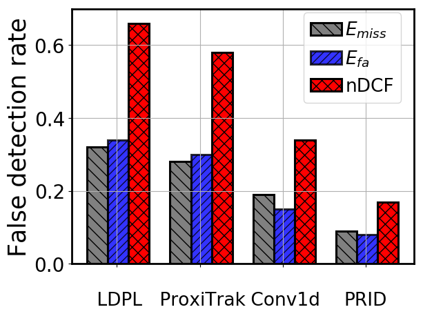
Figure 10: Classification performance for contact tracing application (proximity threshold is 2m).

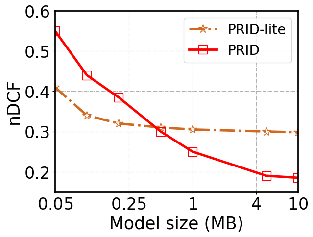
Figure 11: nDCF against different model size of PRID and PRID-lite.

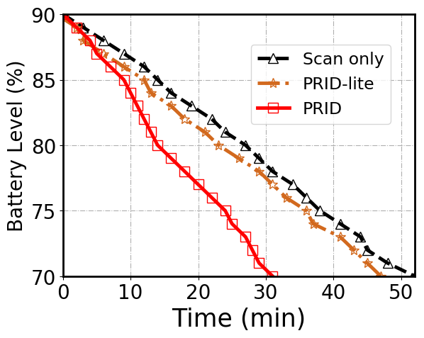
Figure 12: Power consumption over time on IoT smartwatch.

TABLE II: Scheme precision/recall under different sites.

Collection				Scheme precision/recall
Environment	Carriage	Y=0	Y=1	LDPL	Conv1d	PRID
Dynamic	Pocket	0.48	0.30	0.64/0.62	0.88/0.76	0.95/0.92
	Hand	0.32	0.5	0.63/0.64	0.78/0.88	0.93/0.95
Semi-dynamic	Pocket	0.36	0.45	0.65/0.66	0.83/0.92	0.94/0.95
	Hand	0.48	0.40	0.68/0.70	0.91/0.82	0.95/0.95
Static	Pocket	0.42	0.38	0.70/0.72	0.91/0.85	0.96/0.95
	Hand	0.38	0.42	0.72/0.71	0.86/0.91	0.96/0.97

We first study the impact of histogram bin size $\delta$ (as in Equation 2) on the F-score. Figure 9 shows that the F-score increases with the bin size when $\delta\leq 4$; then, the F-score drops when bin size increases. This is because that histogram with a larger bin is less sparse, providing stable features to the proximity classifier to capture; but a histogram with a too large of a bin size is insensitive to RSSI fluctuation distribution change, so it cannot represent the multipath environment well. Therefore, we follow the figure trend and adopt $\delta=4$ in the following experiments.

Figure 9 compares the F-score of different schemes under varied window lengths (in terms of time) in our on-field experiment. We train and test data from the three sites together. In the figure, PRID outperforms the other schemes by more than 0.13 in the F-score (or reduces in over 60% of the false detection cases). We can see that PRID and Conv1d gain significant improvements when the window length increases from 1s to 5s, then after that, they level out. ProxiTrak and LDPL, on the other hand, do not benefit much from temporal information. This is because the RSSI sliding window contains environmental features, and the DNN-based methods are able to extract them. Thus, to balance the system accuracy and responsiveness, we set the window length to be 5s in both PRID and PRID-lite.

With the 5s window, we further show the system performance upon the three sites in Figure 9. As mentioned, the dynamic environment is crowded with pedestrians, the semi-dynamic environment is relatively less crowded, and the static site has quiet surroundings; Therefore, these sites possess environmental dynamics and hence some multipath effects to different extents. As a result, all the schemes suffer accuracy loss from static to dynamic environments because of RSSI fluctuation. Nonetheless, across different sites, the negligible accuracy changes of PRID shows its robustness to RSSI fluctuation since it captures the multipath environment by RSSI histogramization.

To study the system’s robustness against IMU data bias, we separately conduct experiments on the three sites. We show scheme precision and recall in Table II. Since ProxiTrak has a similar trend to LDPL, we only show PRID, Conv1d, and LDPL to avoid redundancy. Due to the multiple collectors and different surroundings, carriage state and proximity state are not independent in each site. From the collection hour shown in the table, the carriage state strongly correlates with the proximity state in the dynamic environment site. This correlation becomes less in the semi-dynamic site and close to being independent in the static site. All the schemes perform better than those training on the three sites together, because training on one specific site makes the models more customized. From the table, LDPL shows inaccuracy since it cannot adapt to the multipath environments and different carriage states. Although Conv1d gets commendable results by considering the carriage state, its accuracy (in terms of precision and recall) is manipulated by IMU data bias. PRID achieves high accuracy and robustness in all sites since it employs the carriage state regularization to tackle IMU overfitting; even in a static site where the carriage and proximity states are close to being decoupled, PRID is still superior to Conv1d. This is because IMU readings reflect device poses, its bias could still exist even though the carriage state is nearly balanced in the training data. Overall, this table shows that PRID is not only robust to IMU data bias but highly reliable under various sites.

Contact tracing is an essential application of proximity detection. Unlike classic PBS systems, contact tracing requires a smaller proximity threshold (2m), rendering it very challenging. To validate system performance in this application, as well as verify the generality (in terms of proximity threshold) of PRID, we conduct experiments under the proximity threshold of 2m. For fair evaluation, we consider the cases collected within a 4-meter distance for training and testing. Figure 12 demonstrates the nDCF of different schemes. All the schemes suffer slight performance declines when the proximity threshold is 2m instead of 6m. This is because the user moving range shrinks from 12m to 4m, introducing severe signal ambiguity – the smaller proximity threshold enlarges the influence of environmental dynamics and carriage states. Nonetheless, PRID reduces the false detection by more than 50% (in terms of nDCF) compared with other schemes.

We evaluate the system performance in terms of nDCF on the TC4TL challenge dataset with our comparison schemes: LDPL (0.82), ProxiTrak (0.73), Conv1d (0.58), and PRID (0.49). In this dataset, since several transmission periods share one ground truth, we apply a majority voting to assemble results from several periods. This dataset is challenging because it crowdsources data from large numbers of users with diverse environments, with its training and test data not necessarily from the same sets of environments or carriage states. It requires not only good adaptability upon diverse environments and carriage states but also generalization ability to new scenarios. Nevertheless, the results show that our scheme achieves the best results among the comparison schemes by reducing more than 15% false detection cases compared with the existing arts. This is because PRID extracts better features from inputs and considers the IMU overfitting problem. This result also verifies the better practicability and reliability of PRID in reality.

TABLE III: IoT hardware specification and computational cost of PRID-Lite.

Hardware	Specification		Computational cost
	CPU Freq.	RAM	Time	Memory usage
Smartwatch	1.5GHz	3GB	$<$1ms	318KB
Pi Zero	1GHz	512MB	4ms	314KB
ESP-32	240MHz	512KB	268ms	309KB

To deploy PRID on extremely resource-constrained devices, we study the system’s performance (in terms of nDCF) with different proximity classifier model sizes of PRID and PRID-lite. It is conducted on our on-field experiment when the proximity threshold is 2m. From Figure 12, PRID nDCF first drops as the model is smaller than $\sim$5MB and then levels out after that. While nDCF of PRID-lite levels out when model is larger than 0.3MB. Note that, PRID-lite outperforms PRID when the model size is less than 0.5MB. This is because the neuron quantity of PRID is so small that the model capacity and generalization ability are constrained. In contrast, PRID-lite sacrifices a percentage of neuron precision for neuron quantity, so it achieves a lower nDCF when the model size is small. However, the binarized neuron causes information loss between network layers, making it hard for PRID-lite to perform as accurately as PRID does when the model size is large enough. From the figure, we adopt the model size of 5MB and 0.3MB for PRID and PRID-lite in our experiment. It shows that PRID-lite reduces 94% memory cost at the expense of 7% accuracy loss in F-score compared with PRID.

We evaluate the energy consumption over time on PRID and PRID-lite, using an IoT smartwatch. The watch is equipped with a lithium polymer built-in battery with a capacity of 800mAh. Except for BLE scanning and proximity detection, we kill all unnecessary processes. The smartwatch conducts one BLE scan per 10 seconds, and each scan lasts for 5 seconds. We record battery levels from 90% to 70% and show them in Figure 12. From the figure, the BLE scan consumes 20% battery energy within around 50 minutes. Scanning while running the PRID takes 30 minutes to use up the same amount of battery power. In comparison, PRID-lite is more energy-efficient as it consumes negligible power except for BLE scanning. Overall, PRID-lite extends battery life by 60% compared to PRID, making it efficient for energy-constrained IoT devices in our experiment.

We finally show in Table III the inference time and memory usage of PRID-lite on different IoT devices. We run PRID-lite 10,000 times on each device and the average time cost as inference time that affects system responsiveness. From the table, even on ESP-32, the platform with the lowest computational power among the devices, PRID-lite costs only 0.3s for each detection. As for memory usage, PRID-lite takes up $\sim$0.3MB memory on all three devices.

VII Conclusion

BLE-based proximity detection plays important roles in many proximity-based services. It relies on the fact that a lower RSSI implies a longer distance, and vice versa. However, RSSI can be markedly affected by multipath and device carriage states in reality. Previous works in the area have not sufficiently considered RSSI fluctuation due to multipath, and how to address carriage states with IMU training data bias to achieve highly accurate and robust proximity detection.

We propose PRID, a novel IMU-assisted BLE proximity detection approach robust against RSSI fluctuation due to multipath and IMU data bias. By representing RSSI fluctuation as a histogram, PRID extracts the features of the multipath environment to encode it as a feature vector. It further encodes the IMU data into carriage feature. Employing a DNN-based binary proximity classifier, PRID then detects proximity after concatenating the vectors. To address biased training data, PRID applies carriage state regularization to the loss function to reduce IMU overfitting of the DNN-based classifier. To make our scheme more deployable on highly resource-constrained IoT devices, we further propose PRID-lite, a lightweight version of PRID using a binarized neural network. We have implemented PRID and PRID-lite in IoT devices. We conduct extensive experiments in several venues and a public dataset and compare them with the state-of-the-arts. Our results show that PRID achieves substantial improvement as compared with the state of the arts (with more than 50% reduction in false detection cases in our dataset). PRID-lite reduces the model size from PRID by 94% (from 5MB to 0.3MB) and extends battery life by more than 60%, with only a minor cost in accuracy (7% reduction in F-score).

References

- [1] P. C. Ng, P. Spachos, and K. Plataniotis, “COVID-19 and Your Smartphone: BLE-based Smart Contact Tracing,” arXiv:2005.13754 [cs], May 2020.
- [2] G. Li, C.-C. Hung, M. Liu, L. Pan, W.-C. Peng, and S.-H. G. Chan, “Spatial-Temporal Similarity for Trajectories with Location Noise and Sporadic Sampling,” in 2021 IEEE 37th International Conference on Data Engineering (ICDE). Chania, Greece: IEEE, Apr. 2021, pp. 1224–1235. [Online]. Available: https://ieeexplore.ieee.org/document/9458932/
- [3] “TraceTogether,” https://www.tracetogether.gov.sg.
- [4] G. F. Hatke, M. Montanari, S. Appadwedula, M. Wentz, J. Meklenburg, L. Ivers, J. Watson, and P. Fiore, “Using Bluetooth Low Energy (BLE) Signal Strength Estimation to Facilitate Contact Tracing for COVID-19,” arXiv:2006.15711 [eess], Jul. 2020.
- [5] D. Zaim and M. Bellafkih, “Bluetooth Low Energy (BLE) based geomarketing system,” in 2016 11th International Conference on Intelligent Systems: Theories and Applications (SITA), Oct. 2016, pp. 1–6.
- [6] Yilang Wu, Junbo Wang, Lei Jing, Yinghui Zhou, and Zixue Cheng, “A CICO system based on BLE proximity,” in 2015 IEEE 7th International Conference on Awareness Science and Technology (iCAST), Sep. 2015, pp. 180–183.
- [7] Y. Cao, X. Lu, Z. Zhao, X. Ji, and Y. Yan, “Distance Estimation Methods in Vehicular Application: An Experimental Study,” in 2018 18th International Conference on Control, Automation and Systems (ICCAS), Oct. 2018, pp. 1752–1757.
- [8] G. Li, S. Hu, S. Zhong, W. L. Tsui, and S.-H. G. Chan, “vcontact: Private wifi-based iot contact tracing with virus lifespan,” IEEE Internet of Things Journal, pp. 1–1, 2021.
- [9] S. He and S.-H. G. Chan, “Sectjunction: Wi-Fi Indoor Localization based on Junction of Signal Sectors,” in Proceedings of IEEE ICC 2014 - Mobile and Wireless Networking Symposium (ICC’14 MWN), Sydney, Australia, Jun. 2014, pp. 2611–2616.
- [10] S. Yoon, J. Woo, J. Cho, and C. Rahm, “An Efficient Distance Estimation Method Based on Bluetooth Low Energy and Ultrasound,” in 2018 IEEE International Conference on Consumer Electronics - Asia (ICCE-Asia), Jun. 2018, pp. 206–212.
- [11] S. Ramasamy, R. Sabatini, A. Gardi, and J. Liu, “Lidar obstacle warning and avoidance system for unmanned aerial vehicle sense-and-avoid,” Aerospace Science and Technology, vol. 55, pp. 344–358, 2016.
- [12] Z. Xiao, H. Wen, A. Markham, N. Trigoni, P. Blunsom, and J. Frolik, “Non-Line-of-Sight Identification and Mitigation Using Received Signal Strength,” IEEE Transactions on Wireless Communications, vol. 14, no. 3, pp. 1689–1702, Mar. 2015.
- [13] Z. Zhou, Z. Yang, C. Wu, W. Sun, and Y. Liu, “LiFi: Line-Of-Sight identification with WiFi,” in IEEE INFOCOM 2014 - IEEE Conference on Computer Communications, Apr. 2014, pp. 2688–2696.
- [14] S. Shankar, R. Kanaparti, A. Chopra, R. Sukumaran, P. Patwa, M. Kang, A. Singh, K. P. McPherson, and R. Raskar, “Proximity Sensing: Modeling and Understanding Noisy RSSI-BLE Signals and Other Mobile Sensor Data for Digital Contact Tracing,” arXiv:2009.04991 [cs, eess], Dec. 2020.
- [15] V. Chandel, S. Banerjee, and A. Ghose, “ProxiTrak: A robust solution to enforce real-time social distancing & contact tracing in enterprise scenario,” in Adjunct Proceedings of the 2020 ACM International Joint Conference on Pervasive and Ubiquitous Computing and Proceedings of the 2020 ACM International Symposium on Wearable Computers. Virtual Event Mexico: ACM, Sep. 2020, pp. 503–511.
- [16] A. R. Jiménez and F. Seco, “Finding objects using UWB or BLE localization technology: A museum-like use case,” in 2017 International Conference on Indoor Positioning and Indoor Navigation (IPIN), Sep. 2017, pp. 1–8.
- [17] National Institute of Standards and Technology (NIST) and MIT PACT project, “TC4TL Challenge,” 2020. [Online]. Available: https://tc4tlchallenge.nist.gov/
- [18] V. Erceg, L. J. Greenstein, S. Y. Tjandra, S. R. Parkoff, A. Gupta, B. Kulic, A. A. Julius, and R. Bianchi, “An empirically based path loss model for wireless channels in suburban environments,” IEEE Journal on Selected Areas in Communications, vol. 17, no. 7, pp. 1205–1211, Jul. 1999.
- [19] C. Phillips, D. Sicker, and D. Grunwald, “A Survey of Wireless Path Loss Prediction and Coverage Mapping Methods,” IEEE Communications Surveys Tutorials, vol. 15, no. 1, pp. 255–270, First 2013.
- [20] M. Al Qathrady and A. Helmy, “Improving BLE Distance Estimation and Classification Using TX Power and Machine Learning: A Comparative Analysis,” in Proceedings of the 20th ACM International Conference on Modelling, Analysis and Simulation of Wireless and Mobile Systems, ser. MSWiM ’17. New York, NY, USA: Association for Computing Machinery, Nov. 2017, pp. 79–83.
- [21] A. Montanari, S. Nawaz, C. Mascolo, and K. Sailer, “A Study of Bluetooth Low Energy performance for human proximity detection in the workplace,” in 2017 IEEE International Conference on Pervasive Computing and Communications (PerCom), Mar. 2017, pp. 90–99.
- [22] A. Maratea, S. Gaglione, A. Angrisano, G. Salvi, and A. Nunziata, “Non parametric and robust statistics for indoor distance estimation through BLE,” in 2018 IEEE International Conference on Environmental Engineering (EE), Mar. 2018, pp. 1–6.
- [23] F. Zafari, I. Papapanagiotou, M. Devetsikiotis, and T. J. Hacker, “Enhancing the accuracy of iBeacons for indoor proximity-based services,” in 2017 IEEE International Conference on Communications (ICC), May 2017, pp. 1–7.
- [24] C. H. Lam, P. C. Ng, and J. She, “Improved Distance Estimation with BLE Beacon Using Kalman Filter and SVM,” in 2018 IEEE International Conference on Communications (ICC), May 2018, pp. 1–6.
- [25] S. Pallavi and V. A. Narayanan, “An Overview of Practical Attacks on BLE Based IOT Devices and Their Security,” in 2019 5th International Conference on Advanced Computing Communication Systems (ICACCS), Mar. 2019, pp. 694–698.
- [26] A. Mackey, P. Spachos, L. Song, and K. N. Plataniotis, “Improving BLE Beacon Proximity Estimation Accuracy Through Bayesian Filtering,” IEEE Internet of Things Journal, vol. 7, no. 4, pp. 3160–3169, Apr. 2020.
- [27] “Procedurally generated environments for simulating RSSI- localization applications — Proceedings of the 20th Communications & Networking Symposium,” https://dl.acm.org/doi/10.5555/3107979.3107986.
- [28] S. Ioffe and C. Szegedy, “Batch Normalization: Accelerating Deep Network Training by Reducing Internal Covariate Shift,” arXiv:1502.03167 [cs], Mar. 2015.
- [29] D. Misra, “Mish: A Self Regularized Non-Monotonic Activation Function,” arXiv:1908.08681 [cs, stat], Aug. 2020.
- [30] A. Apicella, F. Donnarumma, F. Isgrò, and R. Prevete, “A survey on modern trainable activation functions,” Neural Networks, vol. 138, pp. 14–32, Jun. 2021.
- [31] I. Goodfellow, Y. Bengio, and A. Courville, Deep Learning. MIT Press, 2016, http://www.deeplearningbook.org.
- [32] J. Chen, S. Wen, and S.-H. G. Chan, “Joint Demosaicking and Denoising in the Wild: The Case of Training Under Ground Truth Uncertainty,” arXiv:2101.04442 [cs, eess], Jan. 2021.
- [33] J. Pearl, “Causal inference in statistics: An overview,” Statistics Surveys, vol. 3, no. none, pp. 96 – 146, 2009. [Online]. Available: https://doi.org/10.1214/09-SS057
- [34] J. Huang, A. Smola, A. Gretton, K. Borgwardt, and B. Schölkopf, “Correcting Sample Selection Bias by Unlabeled Data.” in Advances in Neural Information Processing Systems 19: Proceedings of the 2006 Conference, 601-608 (2007), vol. 19, Jan. 2006, pp. 601–608.
- [35] Boyd, Vandenberghe, and Faybusovich, “Convex optimization,” IEEE transactions on automatic control, vol. 51, no. 11, pp. 1859–1859, 2006.
- [36] M. Courbariaux, I. Hubara, D. Soudry, R. El-Yaniv, and Y. Bengio, “Binarized Neural Networks: Training Deep Neural Networks with Weights and Activations Constrained to +1 or -1,” arXiv:1602.02830 [cs], Mar. 2016.