Microlocal properties of seven-dimensional lemon and apple Radon transforms with applications in Compton scattering tomography
 

Abstract.

We present a microlocal analysis of two novel Radon transforms of interest in Compton Scattering Tomography (CST), which map compactly supported $L^{2}$ functions to their integrals over seven-dimensional sets of apple and lemon surfaces. Specifically, we show that the apple and lemon transforms are elliptic Fourier Integral Operators (FIO), which satisfy the Bolker condition. After an analysis of the full seven-dimensional case, we focus our attention on $n$-D subsets of apple and lemon surfaces with fixed central axis, where $n<7$. Such subsets of surface integrals have applications in airport baggage and security screening. When the data dimensionality is restricted, the apple transform is shown to violate the Bolker condition, and there are artifacts which occur on apple-cylinder intersections. The lemon transform is shown to satisfy the Bolker condition, when the support of the function is restricted to the strip $\left\{0<z<1\right\}$.

1. Introduction

In this paper, we present a novel microlocal analysis of two Radon transforms of interest in CST, which take the integrals of a function over seven dimensional sets of lemon and apple surfaces. A “lemon” (also called a “spindle” in some works [25, 18, 24]) refers to the interior part of a spindle (or self-intersecting) torus, and an “apple” is the exterior. See figure 1 for a 2-D cross-section of a spindle torus, where we have highlighted the lemon and apple parts.

Figure 1. 2-D cross section of a spindle torus centered on the origin, with axis of revolution $y$. The lemon cross-section is the intersection of the interior of the dashed circle with the torus cross-section. The apple cross section is the intersection of the torus cross-section with the exterior of the dashed circle. The lemon/apple is the surface of revolution of the lemon/apple cross-section about $y$.

The literature considers lemon and apple transforms in 3-D CST [24, 25, 18, 23, 16, 17, 2], where the goal is to reconstruct an electron density map from Compton scattered photons. There is also a growing interest in the literature in Emission CST (ECST) [22, 9, 14, 13, 12], where the aim is to reconstruct a gamma ray source from cone integral data.

In [17], two fixed-source CST configurations, with spherical and cylindrical detector arrays, are considered. In both cases, the data is three dimensional, and consists of a two-dimensional detector coordinate and a one-dimensional energy variable. Due to limited energy resolution, the fixed source position, and the shape of the detector surface, the data is incomplete. For example, the cylindrical acquisition geometry suffers limited angle issues. In such cases of limited data, the reconstruction becomes unstable, and there are image artifacts. The authors go on to develop a modified Kaczmarz algorithm to combat the reconstruction artifacts and test their algorithm on simulated examples with Poisson noise. Similar reconstruction instabilities can be seen also in, e.g., conventional X-ray CT with limited angle data [1, 10, 11].

Figure 2.

In [24], the authors present a microlocal analysis of the lemon transform introduced in [25]. The acquisition geometry consists of a single rotating source and detector on a fixed axis. As in [17], the data is three-dimensional, and, in this case, consists of a 2-D rotation and a 1-D energy variable. The lemon transform is shown to violate the Bolker condition, and there are artifacts induced by flowout which appear as a spherical blurring effect in the reconstruction. There are also invisible singularities near the origin due to limited energy resolution. In [25], an algebraic reconstruction method is proposed to invert the lemon transform. Here artifacts are observed in reconstructions with noisy data, in line with the theory of [24].

In [2], the authors introduce a scanning modality in 3-D CST using a fixed source and single rotating detector restricted to a spherical surface. The data, in this case, has three degrees of freedom, and consists of a 2-D detector rotation and a 1-D energy variable. The authors model the Compton scatter intensity using a new apple Radon transform, and they derive an explicit inversion formula using a spherical harmonic expansion and Volterra integral equation theory. Additionally, a hybrid analytic/algebraic reconstruction algorithm is presented and tested on simulated phantoms with added pseudo random noise. The authors discover blurring artifacts in the reconstructions, which indicate instabilities due to limited data, as is, for example, discovered in [17].

In the works discussed above, a number of imaging modalities are introduced based on practical machine designs, and the data dimension is such that the reconstruction target is determined. That is, the reconstruction target and data are both three-dimensional. The set of spindle tori in 3-D space is seven-dimensional, and hence the literature thus far considers only limited data problems in CST, i.e., 3-D subsets of the full 7-D set of tori are considered. This often leads to artifacts and instabilities in the reconstruction due to, for example, limited angles (as in [17]) and failure to satisfy the Bolker condition [24]. In this paper, we wish to investigate the problem instability and presence of artifacts when there are no limits to the data dimensionality in CST, and we have knowledge of a seven-dimensional set of apple and lemon integrals in 3-D space. This can be considered a best case scenario in CST in terms of data dimensionality. Specifically, we consider the scanning geometry illustrated in figure 2. Here, we have shown an $(x,y)$ plane cross-section of the scanning geometry. The scanning target ($f$) is supported on the open unit ball and is illustrated by an uneven red boundary. Example lemon and apple cross sections are drawn in blue, with centers ${\mathbf{x}}^{(1)}_{0}$ and ${\mathbf{x}}^{(2)}_{0}$, and axis of rotation ${\boldsymbol{\xi}}_{1}$ and ${\boldsymbol{\xi}}_{2}$, respectively. The apple radius is denoted by $r$, and the distance from ${\mathbf{x}}^{(2)}_{0}$ to the center of the apple tube is denoted by $t$. We consider the apple and lemon surfaces whose points of self-intersection (which we will call singular points) lie outside the open unit ball. We do this to avoid singularities in the apple/lemon surface measure. In CST, the singular points of the lemons and apples correspond to source and detector coordinates. So, in the context of CST, our geometry consists of all source and detector positions which lie outside the unit ball (this is a six-dimensional set). Additionally, we can vary the torus radius ($r$), which in CST is equivalent to the photon energy [17]. Thus, in total, our data set is seven-dimensional.

Motivated by the geometry of figure 2, we introduce novel lemon and apple Radon transforms, which map $f$ to its integrals over seven-dimensional sets of apple and lemon surfaces. Our main theorem proves that the lemon and apple transforms are elliptic FIO which satisfy the Bolker condition. Additionally, we consider the practical applications of our theory to other scanning geometries from the literature. Specifically, we consider the scanning geometry of [27], which is designed for use in airport baggage screening, and discuss the microlocal properties of lemon and apple transforms which induce translation on the scanning target.

The remainder of this paper is organized as follows. In section 2, we give some preliminary definitions and theorems that will be used in our analysis. In section 3, we introduce novel lemon and apple transforms, which map compactly supported $L^{2}$ functions to their integrals over seven-dimensional sets of lemon and apple surfaces, respectively, as pictured in figure 2. Here we prove our main theorem, which shows that the lemon and apple transforms are elliptic FIO which satisfy the Bolker condition. In section 4, we consider a practical scanning geometry in CST, first introduced in [27], and discuss the artifacts in lemon and apple integral reconstructions when the axis of revolution of the lemons$\backslash$apples is fixed, and the target function undergoes a 2-D translation.

2. Definitions and preliminary theorems

We next provide some notation and definitions. Let $X$ and $Y$ be open subsets of ${{\mathbb{R}}^{n}}$. Let $\mathcal{D}(X)$ be the space of smooth functions compactly supported on $X$ with the standard topology and let $\mathcal{D}^{\prime}(X)$ denote its dual space, the vector space of distributions on $X$. Let $\mathcal{E}(X)$ be the space of all smooth functions on $X$ with the standard topology and let $\mathcal{E}^{\prime}(X)$ denote its dual space, the vector space of distributions with compact support contained in $X$. Finally, let $\mathcal{S}({{\mathbb{R}}^{n}})$ be the space of Schwartz functions, that are rapidly decreasing at $\infty$ along with all derivatives. See [19] for more information.

For a function $f$ in the Schwartz space $\mathcal{S}(\mathbb{R}^{n})$ or in $L^{2}({{\mathbb{R}}^{n}})$, we use $\mathcal{F}f$ and $\mathcal{F}^{-1}f$ to denote the Fourier transform and inverse Fourier transform of $f$, respectively (see [6, Definition 7.1.1]). Note that $\mathcal{F}^{-1}\mathcal{F}f({\mathbf{x}})=\frac{1}{(2\pi)^{n}}\int_{{\mathbf{y}}\in{{\mathbb{R}}^{n}}}\int_{{\mathbf{z}}\in{{\mathbb{R}}^{n}}}\exp(({\mathbf{x}}-{\mathbf{z}})\cdot{\mathbf{y}})\,f({\mathbf{z}})\,\mathrm{d}{\mathbf{z}}\,\mathrm{d}{\mathbf{y}}$.

We use the standard multi-index notation: if $\alpha=(\alpha_{1},\alpha_{2},\dots,\alpha_{n})\in\left\{0,1,2,\dots\right\}^{n}$ is a multi-index and $f$ is a function on ${{\mathbb{R}}^{n}}$, then

$$\partial^{\alpha}f=\left(\frac{\partial}{\partial x_{1}}\right)^{\alpha_{1}}\left(\frac{\partial}{\partial x_{2}}\right)^{\alpha_{2}}\cdots\left(\frac{\partial}{\partial x_{n}}\right)^{\alpha_{n}}f.$$

If $f$ is a function of $({\mathbf{y}},{\mathbf{x}},\mathbf{s})$ then $\partial^{\alpha}_{\mathbf{y}}f$ and $\partial^{\alpha}_{\mathbf{s}}f$ are defined similarly.

We identify cotangent spaces on Euclidean spaces with the underlying Euclidean spaces, so we identify $T^{*}(X)$ with $X\times{{\mathbb{R}}^{n}}$.

If $\phi$ is a function of $({\mathbf{y}},{\mathbf{x}},\mathbf{s})\in Y\times X\times{{\mathbb{R}}}^{N}$ then we define $\mathrm{d}_{{\mathbf{y}}}\phi=\left(\frac{\partial\phi}{\partial y_{1}},\frac{\partial\phi}{\partial y_{2}},\cdots,\frac{\partial\phi}{\partial y_{n}}\right)$, and $\mathrm{d}_{\mathbf{x}}\phi$ and $\mathrm{d}_{\mathbf{s}}\phi$ are defined similarly. We let $\mathrm{d}\phi=\left(\mathrm{d}_{{\mathbf{y}}}\phi,\mathrm{d}_{{\mathbf{x}}}\phi,\mathrm{d}_{\mathbf{s}}\phi\right)$.

We use the convenient notation that if $A\subset{{\mathbb{R}}}^{m}$, then $\dot{A}=A\setminus\{\mathbf{0}\}$.

The singularities of a function and the directions in which they occur are described by the wavefront set [4, page 16]:

Definition 2.1.

Let $X$ Let an open subset of ${{\mathbb{R}}^{n}}$ and let $f$ be a distribution in $\mathcal{D}^{\prime}(X)$. Let $({\mathbf{x}}_{0},{\boldsymbol{\xi}}_{0})\in X\times{\dot{{\mathbb{R}}^{n}}}$. Then $f$ is smooth at ${\mathbf{x}}_{0}$ in direction ${\boldsymbol{\xi}_{0}}$ if there exists a neighborhood $U$ of ${\mathbf{x}}_{0}$ and $V$ of ${\boldsymbol{\xi}}_{0}$ such that for every $\phi\in\mathcal{D}(U)$ and $N\in\mathbb{R}$ there exists a constant $C_{N}$ such that for all ${\boldsymbol{\xi}}\in V$,

(2.1) $$\left|\mathcal{F}(\phi f)(\lambda{\boldsymbol{\xi}})\right|\leq C_{N}(1+\left|\lambda\right|)^{-N}.$$

The pair $({\mathbf{x}}_{0},{\boldsymbol{\xi}_{0}})$ is in the wavefront set, $\mathrm{WF}(f)$, if $f$ is not smooth at ${\mathbf{x}}_{0}$ in direction ${\boldsymbol{\xi}_{0}}$.

This definition follows the intuitive idea that the elements of $\mathrm{WF}(f)$ are the point–normal vector pairs above points of $X$ at which $f$ has singularities. For example, if $f$ is the characteristic function of the unit ball in $\mathbb{R}^{3}$, then its wavefront set is $\mathrm{WF}(f)=\{({\mathbf{x}},t{\mathbf{x}}):{\mathbf{x}}\in S^{2},t\neq 0\}$, the set of points on a sphere paired with the corresponding normal vectors to the sphere.

The wavefront set of a distribution on $X$ is normally defined as a subset the cotangent bundle $T^{*}(X)$ so it is invariant under diffeomorphisms, but we do not need this invariance, so we will continue to identify $T^{*}(X)=X\times{{\mathbb{R}}^{n}}$ and consider $\mathrm{WF}(f)$ as a subset of $X\times{\dot{{\mathbb{R}}^{n}}}$.

Definition 2.2 ([6, Definition 7.8.1]).

We define $S^{m}(Y\times X\times\mathbb{R}^{N})$ to be the set of $a\in\mathcal{E}(Y\times X\times\mathbb{R}^{N})$ such that for every compact set $K\subset Y\times X$ and all multi–indices $\alpha,\beta,\gamma$ the bound

$$\left|\partial^{\gamma}_{{\mathbf{y}}}\partial^{\beta}_{{\mathbf{x}}}\partial^{\alpha}_{{\boldsymbol{\sigma}}}a({\mathbf{y}},{\mathbf{x}},{\boldsymbol{\sigma}})\right|\leq C_{K,\alpha,\beta,\gamma}(1+\left\lVert{\boldsymbol{\sigma}}\right\rVert)^{m-|\alpha|},\ \ \ ({\mathbf{y}},{\mathbf{x}})\in K,\ {\boldsymbol{\sigma}}\in\mathbb{R}^{N},$$

holds for some constant $C_{K,\alpha,\beta,\gamma}>0$.

The elements of $S^{m}$ are called symbols of order $m$. Note that these symbols are sometimes denoted $S^{m}_{1,0}$. The symbol $a\in S^{m}(Y,X,{{\mathbb{R}}}^{N})$ is elliptic if for each compact set $K\subset Y\times X$, there is a $C_{K}>0$ and $M>0$ such that

(2.2) $$\left|a({\mathbf{y}},{\mathbf{x}},{\boldsymbol{\sigma}})\right|\geq C_{K}(1+\left\lVert{\boldsymbol{\sigma}}\right\rVert)^{m},\ \ \ ({\mathbf{y}},{\mathbf{x}})\in K,\ \left\lVert{\boldsymbol{\sigma}}\right\rVert\geq M.$$

Definition 2.3 ([7, Definition 21.2.15]).

A function $\phi=\phi({\mathbf{y}},{\mathbf{x}},{\boldsymbol{\sigma}})\in\mathcal{E}(Y\times X\times\dot{\mathbb{R}^{N}})$ is a phase function if $\phi({\mathbf{y}},{\mathbf{x}},\lambda{\boldsymbol{\sigma}})=\lambda\phi({\mathbf{y}},{\mathbf{x}},{\boldsymbol{\sigma}})$, $\forall\lambda>0$ and $\mathrm{d}\phi$ is nowhere zero. The critical set of $\phi$ is

$$\Sigma_{\phi}=\{({\mathbf{y}},{\mathbf{x}},{\boldsymbol{\sigma}})\in Y\times X\times\dot{\mathbb{R}^{N}}:\mathrm{d}_{{\boldsymbol{\sigma}}}\phi=0\}.$$

A phase function is clean if the critical set $\Sigma_{\phi}=\{({\mathbf{y}},{\mathbf{x}},{\boldsymbol{\sigma}})\ :\ \mathrm{d}_{\boldsymbol{\sigma}}\phi({\mathbf{y}},{\mathbf{x}},{\boldsymbol{\sigma}})=0\}$ is a smooth manifold with tangent space defined as the kernel of $d\,(d_{\sigma}\phi)$ on $\Sigma_{\phi}$. Here, the derivative $\mathrm{d}$ is applied component-wise to the vector-valued function $d_{\sigma}\phi$. So, $d\,(d_{\sigma}\phi)$ is treated as a Jacobian matrix of dimensions $N\times(2n+N)$.

By the Constant Rank Theorem the requirement for a phase function to be clean is satisfied if $\mathrm{d}\left(\mathrm{d}_{\boldsymbol{\sigma}}\phi\right)$ has constant rank.

Definition 2.4 ([7, Definition 21.2.15] and [8, section 25.2]).

Let $X$ and $Y$ be open subsets of ${{\mathbb{R}}^{n}}$. Let $\phi\in\mathcal{E}\left(Y\times X\times{{{\mathbb{R}}}}^{N}\right)$ be a clean phase function. In addition, we assume that $\phi$ is nondegenerate in the following sense:

$$\mathrm{d}_{{\mathbf{y}}}\phi \mathrm{d}_{{\mathbf{x}}}\phi \Sigma_{\phi}$$ and are never zero on .

The canonical relation parametrized by $\phi$ is defined as

(2.3) $$\mathcal{C}= \left\{\left(\left({\mathbf{y}},\mathrm{d}_{{\mathbf{y}}}\phi({\mathbf{y}},{\mathbf{x}},{\boldsymbol{\sigma}})\right);\left({\mathbf{x}},-\mathrm{d}_{{\mathbf{x}}}\phi({\mathbf{y}},{\mathbf{x}},{\boldsymbol{\sigma}})\right)\right):({\mathbf{y}},{\mathbf{x}},{\boldsymbol{\sigma}})\in\Sigma_{\phi}\right\},$$

Definition 2.5.

Let $X$ and $Y$ be open subsets of ${{\mathbb{R}}^{n}}$. Let an operator $A:\mathcal{D}(X)\to\mathcal{D}^{\prime}(Y)$ be defined by the distribution kernel $K_{A}\in\mathcal{D}^{\prime}(X\times Y)$, in the sense that $Af({\mathbf{y}})=\int_{X}K_{A}({\mathbf{x}},{\mathbf{y}})f({\mathbf{x}})\mathrm{d}{\mathbf{x}}$. Then we call $K_{A}$ the Schwartz kernel of $A$. A Fourier integral operator (FIO) of order $m+N/2-n/2$ is an operator $A:\mathcal{D}(X)\to\mathcal{D}^{\prime}(Y)$ with Schwartz kernel given by an oscillatory integral of the form

(2.4) $$K_{A}({\mathbf{y}},{\mathbf{x}})=\int_{\mathbb{R}^{N}}e^{i\phi({\mathbf{y}},{\mathbf{x}},{\boldsymbol{\sigma}})}a({\mathbf{y}},{\mathbf{x}},{\boldsymbol{\sigma}})\mathrm{d}{\boldsymbol{\sigma}},$$

where $\phi$ is a clean nondegenerate phase function and $a$ is a symbol in $S^{m}(Y\times X\times\mathbb{R}^{N})$. The canonical relation of $A$ is the canonical relation of $\phi$ defined in (2.3).

The FIO $A$ is elliptic if its symbol is elliptic.

This is a simplified version of the definition of FIO in [3, section 2.4] or [8, section 25.2] that is suitable for our purposes since our phase functions are global. Because we assume phase functions are nondegenerate, our FIO can be defined as maps from $\mathcal{E}^{\prime}(X)$ to $\mathcal{D}^{\prime}(Y)$ and sometimes on larger domains. For general information about FIOs, see [3, 8, 7]. For information about the Schwartz Kernel, see [6, Theorem 5.1.9].

.

Let $X$ and $Y$ be sets and let $\Omega_{1}\subset X$ and $\Omega_{2}\subset Y\times X$. The composition $\Omega_{2}\circ\Omega_{1}$ and transpose $\Omega_{2}^{t}$ of $\Omega_{2}$ are defined

$$\Omega_{2}\circ\Omega_{1} =\left\{y\in Y\hskip 0.85358pt:\hskip 0.85358pt\exists x\in\Omega_{1},\ (y,x)\in\Omega_{2}\right\}$$

$$\Omega_{2}^{t} =\left\{(x,y)\hskip 0.85358pt:\hskip 0.85358pt(y,x)\in\Omega_{2}\right\}.$$

The Hörmander-Sato Lemma provides the relationship between the wavefront set of distributions and their images under FIO.

Theorem 2.6 ([6, Theorem 8.2.13]).

Let $f\in\mathcal{E}^{\prime}(X)$ and let ${A}:\mathcal{E}^{\prime}(X)\to\mathcal{D}^{\prime}(Y)$ be an FIO with canonical relation $\mathcal{C}$. Then, $\mathrm{WF}({A}f)\subset\mathcal{C}\circ\mathrm{WF}(f)$.

Definition 2.7.

Let $\mathcal{C}\subset T^{*}(Y\times X)$ be the canonical relation associated to the FIO ${A}:\mathcal{E}^{\prime}(X)\to\mathcal{D}^{\prime}(Y)$. We let $\Pi_{L}$ and $\Pi_{R}$ denote the natural left- and right-projections of $\mathcal{C}$, projecting onto the appropriate coordinates: $\Pi_{L}:\mathcal{C}\to T^{*}(Y)$ and $\Pi_{R}:\mathcal{C}\to T^{*}(X)$.

Because $\phi$ is nondegenerate, the projections do not map to the zero section.

Let $A$ be an FIO with adjoint $A^{*}$. If $A$ satisfies our next definition, then $A^{*}A$ (or, if $A$ does not map to $\mathcal{E}^{\prime}(Y)$, then $A^{*}\psi A$ for an appropriate cutoff $\psi$) is a pseudodifferential operator [5, 15].

Definition 2.8.

Let ${A}:\mathcal{E}^{\prime}(X)\to\mathcal{D}^{\prime}(Y)$ be a FIO with canonical relation $\mathcal{C}$ then $A$ (or $\mathcal{C}$) satisfies the semi-global Bolker Condition if the natural projection $\Pi_{L}:\mathcal{C}\to T^{*}(Y)$ is an embedding (injective immersion).

Theorem 2.9 (Sylvester’s Determinant Theorem (SDT) [20, 21]).

Let $A$ be an $m\times n$ matrix, and $B$ an $n\times m$ matrix. Then

$$\text{det}\left(I_{m\times m}+AB\right)=\text{det}\left(I_{n\times n}+BA\right).$$

3. Analysis of seven-dimensional lemon and apple Radon transforms

In this section, we present a microlocal analysis of two new Radon transforms which map compactly supported $L^{2}$ functions to their integrals over seven-dimensional sets of lemon and apple surfaces. First, we give the defining equations for the apple and lemon surfaces.

Spindle tori are described by their center, ${{\mathbf{x}_{0}}}\in{{\mathbb{R}}^{3}}$, their axis of revolution, and parameters $s$ and $t$; $\sqrt{s}$ is the radius and $t$ is the tube radius of the spindle torus. If $\ell$ is a line through the origin parallel to the axis of revolution of a spindle torus, then for some $\omega\in S^{2}$, one can write

$$\ell={{\mathbb{R}}}\omega:=\left\{\nu\omega\hskip 0.85358pt:\hskip 0.85358pt\nu\in{{\mathbb{R}}}\right\}$$

and the axis of revolution of the torus is ${{\mathbf{x}_{0}}}+\ell$. We will call this line $\ell$ the directional axis of the spindle torus (equivalently, of the apple or lemon).

We will use rotation matrices to describe the directional axes of spindle tori. Let $(\alpha,\beta)\in[0,2\pi]\times[0,\pi/2]$. Then, we define

(3.1) $$R=R(\alpha,\beta) =\begin{pmatrix}\cos\alpha&-\sin\alpha&0\\ \sin\alpha&\cos\alpha&0\\ 0&0&1\end{pmatrix}\begin{pmatrix}1&0&0\\ 0&\cos\beta&-\sin\beta\\ 0&\sin\beta&\cos\beta\end{pmatrix}$$

$$=\begin{pmatrix}\cos\alpha&-\sin\alpha\cos\beta&\sin\alpha\sin\beta\\ \sin\alpha&\cos\alpha\cos\beta&-\cos\alpha\sin\beta\\ 0&\sin\beta&\cos\beta\end{pmatrix}.$$

Let

(3.2) $${\mathbf{x}}=(x,y,z),\ \ \ \ {\mathbf{x}}_{0}=(x_{0},y_{0},z_{0}),\ \ {\mathbf{x}}_{T}={\mathbf{x}}-{\mathbf{x}}_{0},\ \ {\mathbf{x}}^{\prime}=(x^{\prime},y^{\prime},z^{\prime})=R^{T}(\alpha,\beta){\mathbf{x}}_{T}$$

and

(3.3) $$h(t,{\mathbf{x}}_{0};{\mathbf{x}})=\left\lVert{\mathbf{x}}_{T}\right\rVert^{2}+t^{2},\ \ \ g(\alpha,{\mathbf{x}}_{0},\beta;{\mathbf{x}})=\sqrt{x^{\prime 2}+y^{\prime 2}}.$$

We now define

(3.4) $$\Psi_{j}(s,t,{\mathbf{x}}_{0},\alpha,\beta;{\mathbf{x}}) :=\left(\sqrt{x^{\prime 2}+y^{\prime 2}}+(-1)^{j}t\right)^{2}+z^{\prime 2}-s$$

$$\phantom{:}=h(t,{\mathbf{x}}_{0};{\mathbf{x}})+2t(-1)^{j}g({\mathbf{x}}_{0},\alpha,\beta;{\mathbf{x}})-s.$$

and

(3.5) $$T_{j}(s,t,{\mathbf{x}}_{0},\alpha,\beta)=\left\{{\mathbf{x}}\in B\hskip 0.85358pt:\hskip 0.85358pt\Psi_{j}(s,t,{\mathbf{x}}_{0},\alpha,\beta;{\mathbf{x}})=0\right\},$$

for $j=1,2$. $\Psi_{1}$ and $\Psi_{2}$ are the defining equations for apple and lemon surfaces, respectively, and $T_{1}$ and $T_{2}$ are the intersections of apples and lemons with $B$. See figure 3 for example 2-D cross sections of apples and lemons with the defining equations highlighted.

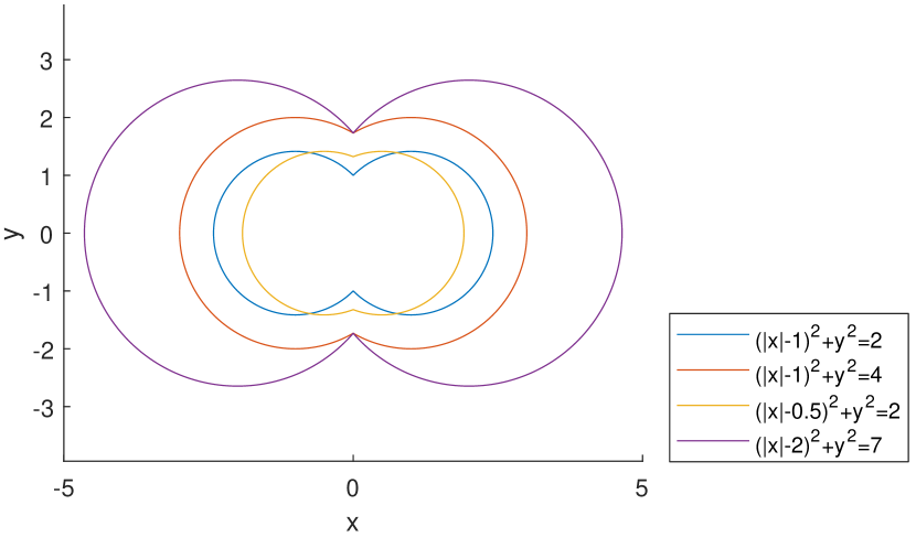
(a) Apples ($j=1$)

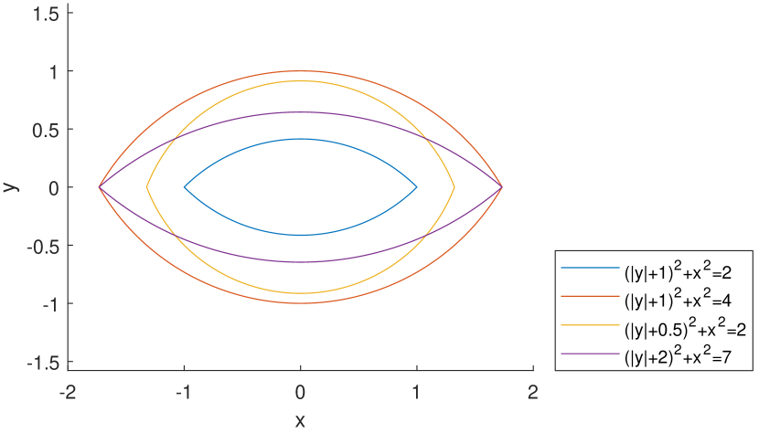
(b) Lemons ($j=2$)

Figure 3. $(x,y)$ plane cross sections of the apple and lemon parts of a spindle torus when $R=R\left(0,\frac{\pi}{2}\right)$ (left) and $R=R\left(\frac{\pi}{2},\frac{\pi}{2}\right)$ (right), ${\mathbf{x}}_{0}=\textbf{0}$, and $s$ and $t$ vary between $\frac{1}{2}$ and $7$.

3.1. Definition of apple and lemon transforms

Throughout this paper, we let $L^{2}_{c}(X)$ denote the set of $L^{2}$ functions compactly supported on $X\subset\mathbb{R}^{3}$. Recall that the two points of intersection of the apple (resp. lemon) with its axis of revolution are called the singular points of the apple (resp. lemon). Note that the singular points are the points of intersection of the apple and lemon with the same parameters in $Y$, and they are singular points of both the apple and lemon. We will define the apple and lemon transforms on functions $f\in L^{2}_{c}(X)$, where $X=B$ is the open unit ball in $\mathbb{R}^{3}$, and we will need to ensure that the singular points of the apple or lemon do not meet the closed unit ball, $\overline{B}$. For this reason, we define

(3.6) $$Y= \Large\{(s,t,{\mathbf{x}}_{0},\alpha,\beta)\in{{\mathbb{R}}^{2}}\times{{\mathbb{R}}^{3}}\times[0,2\pi]\times\left[0,\pi/2\right]$$

$$\quad:s>t^{2},\{{\mathbf{x}}_{0}\pm\sqrt{s-t^{2}}R(\alpha,\beta)\mathbf{e}_{3}\}\cap\overline{B}=\emptyset\Large\},$$

where $\mathbf{e}_{3}=(0,0,1)^{T}$ is the north pole. Note that every apple (for $j=1$) and lemon (for $j=2$) with singular points not meeting $\overline{B}$ can be written $T_{j}(s,t,{{\mathbf{x}_{0}}},\alpha,\beta)$ for some $(s,t,{{\mathbf{x}_{0}}},\alpha,\beta)\in Y$ because all directional axes are generated by the map

(3.7) $$[0,2\pi]\times[0,\pi/2]\ni(\alpha,\beta)\mapsto{{\mathbb{R}}}R(\alpha,\beta)\mathbf{e}_{3}.$$

Remark 3.1.

This map (3.7) from $(\alpha,\beta)$ to directional axes is not injective for $\beta=0,\pi/2$. Therefore, we cannot use $[0,2\pi]\times[0,\pi/2]$ to parameterize direction axes, as it would cause issue later in the proofs of our main theorems. Furthermore, our parameter space $Y$ in (3.6) is not a manifold without boundary because $[0,\pi/2]$ is not a manifold without boundary. Note that we are identifying $0$ and $2\pi$ to transform $[0,2\pi]$ to the manifold $S^{1}$.

At the start of the proof of Theorem 3.2, we will define a parameter set for spindle tori that is a manifold without boundary for which the map to spindle tori (with singular points outside $\overline{B}$) is bijective. These properties are required to use the standard microlocal analysis of Radon transforms (e.g., see [5]). However, we will parameterize spindle tori using $Y$ when appropriate.

We define the Radon transforms which take the integrals of $f$ over apple ($j=1$) and lemon ($j=2$) surfaces

(3.8) $$\begin{split}\mathcal{R}_{j}f(s,t,{\mathbf{x}}_{0},\alpha,\beta)&=\int_{X}\left\lVert\nabla_{{\mathbf{x}}}\Psi_{j}\right\rVert\delta\left(\Psi_{j}(s,t,{\mathbf{x}}_{0},\alpha,\beta;{\mathbf{x}})\right)f({\mathbf{x}})\mathrm{d}{\mathbf{x}}\\ &=\int_{-\infty}^{\infty}\int_{X}\left\lVert\nabla_{{\mathbf{x}}}\Psi_{j}\right\rVert e^{\sigma\Psi_{j}(s,t,{\mathbf{x}}_{0},\alpha,\beta;{\mathbf{x}})}f({\mathbf{x}})\mathrm{d}{\mathbf{x}}\mathrm{d}\sigma,\end{split}$$

and we let

$$\mathcal{A}f=\mathcal{R}_{1}f,\ \ \ \ \ \ \mathcal{L}f=\mathcal{R}_{2}f$$

where $\mathcal{A}$ is called the apple transform, and $\mathcal{L}$ is the lemon transform.

Here, we will assume the gradient of a scalar valued function is a column vector, as are elements of ${{\mathbb{R}}^{n}}$.

To ensure that $T_{j}(s,t,{{\mathbf{x}_{0}}},\alpha,\beta)$ is a smooth manifold and that the weight $\left\lVert\nabla_{{\mathbf{x}}}\Psi_{j}\right\rVert$ in (3.8) is defined, we have defined $Y$ so that it includes only the apple and lemon surfaces whose singular points do not intersect $X=B$. This way, in the integrals of (3.8), we stay away from the singular points of the apples and lemons, and any singularities in the FIO amplitudes and phases. Strictly speaking, one would add a smooth cutoff to the symbol which is zero close to the central axis of the spindle tori, as in [26, Lemma 3.3], so the amplitude is smooth everywhere and the phase is smooth near the support of the amplitude. However, we do not go into such technicalities here.

Now that the apple and lemon transforms are defined we present a separate microlocal analysis of each transform in the following sections.

3.2. Microlocal properties of $\mathcal{A}$; the $j=1$ case

Here we discuss the microlocal properties of the apple transform $\mathcal{A}$. Our first theorem proves that $\mathcal{A}$ is an elliptic FIO.

Theorem 3.2.

The apple transform $\mathcal{A}=\mathcal{R}_{1}$ of (3.8) is an elliptic FIO order $-2$ from domain $\mathcal{E}^{\prime}(B)$ to $\mathcal{D}^{\prime}(Y)$.

Proof.

To analyze $\mathcal{A}$ as an FIO, we need to parametrize apples using a manifold without boundary, as discussed in Remark 3.1. However, $Y$ cannot be used, since it is not a manifold without boundary since $[0,\pi/2]$ has boundary points $0,\pi/2$. To get around this, we first parametrize all spindle tori in a global way as a manifold without boundary. This is required to use the theory of Radon transforms as FIO [5]. To define this manifold, we parametrize spindle tori by points ${\mathbf{y}}=(s,t,{{\mathbf{x}_{0}}},\ell)$, as discussed at the start of this section, where $\sqrt{s}$ is the radius, $t$ is the tube radius of the spindle torus, ${{\mathbf{x}_{0}}}$ is its center, and $\ell$ is the directional axis. Recall that the directional axis of a spindle torus is the line through the origin in ${{\mathbb{R}}^{3}}$, which is parallel to the axis of revolution of the torus, ${{\mathbf{x}_{0}}}+\ell$. The set of lines through the origin in ${{\mathbb{R}}^{3}}$ is denoted $\mathbb{RP}^{2}$ and is called the two-dimensional real projective space.

We let $\widetilde{Y}$ be the set of ${\mathbf{y}}=(s,t,{{\mathbf{x}_{0}}},\ell)$ such that the singular points of the spindle torus parameterized by ${\mathbf{y}}$ do not meet $\overline{B}$. Then, $\widetilde{Y}$ is a manifold without boundary that parameterizes all apples ($j=1$) and all lemons ($j=2$) the singular points of which do not meet $\overline{B}$ by the map

(3.9) $$\begin{gathered}\widetilde{Y}\ni(s,t,{{\mathbf{x}_{0}}},\ell)\mapsto T_{j}(s,t,{{\mathbf{x}_{0}}},\alpha,\beta)\\ \text{when $(\alpha,\beta)$ is chosen so that}\\ \ell={{\mathbb{R}}}R(\alpha,\beta)\mathbf{e}_{3}.\end{gathered}$$

Note that the map in (3.9) and $\mathcal{A}f$ are well-defined on $\widetilde{Y}$ because the spindle torus and its measure are the same no matter which $(\alpha,\beta)$ one chooses that satisfies $\ell={{\mathbb{R}}}R(\alpha,\beta)\mathbf{e}_{3}$. This is true by rotation invariance of the spindle torus about its axis of revolution, ${{\mathbf{x}_{0}}}+\ell$ and rotation invariance of the integral over the torus. Furthermore, every spindle torus is described by a unique $(s,t,{{\mathbf{x}_{0}}},\ell)$.

To get local coordinates on $\widetilde{Y}$, we need to specify local coordinates on $\mathbb{RP}^{2}$, since $(s,t,{{\mathbf{x}_{0}}})$ are already coordinates. We choose a vertical axis and let $\mathbf{e}_{3}$ be the unit vector pointing in the positive direction along that axis. Then, we let $\mathbf{e}_{1}$ and $\mathbf{e}_{2}$ be orthogonal unit vectors so $(\mathbf{e}_{1},\mathbf{e}_{2},\mathbf{e}_{3})$ form a right-hand coordinate system in ${{\mathbb{R}}^{3}}$. Now, we define the domain of the coordinate map

(3.10) $$Y^{\prime}=\left\{(s,t,{{\mathbf{x}_{0}}},\alpha,\beta)\in Y\hskip 0.85358pt:\hskip 0.85358pt\beta\in(0,\pi/2)\right\}.$$

Then, local coordinates on $\widetilde{Y}$ are given by

(3.11) $$Y^{\prime}\ni(s,t,{{\mathbf{x}_{0}}},\alpha,\beta)\mapsto(s,t,{{\mathbf{x}_{0}}},{{\mathbb{R}}}R(\alpha,\beta)\mathbf{e}_{3}).$$

For different choices of basis $(\mathbf{e}_{1},\mathbf{e}_{2},\mathbf{e}_{3})$ on ${{\mathbb{R}}^{3}}$ with vertical axis in direction of $\mathbf{e}_{3}$, this coordinate map describes a coordinate chart on $\widetilde{Y}$.

We will work in these coordinates and use the notation (3.1)-(3.4), and (3.8) for the rest of this section.

From (3.8), the phase function of $\mathcal{R}_{1}$ is

$$\Phi_{1}(s,t,{\mathbf{x}}_{0},\alpha,\beta;{\mathbf{x}};\sigma)=\sigma\Psi_{1}(s,t,{\mathbf{x}}_{0},\alpha,\beta;{\mathbf{x}}).$$

We now show that $\Phi_{1}$ is clean, non-degenerate and homogeneous in $\sigma$ order 1, so that $\mathcal{A}$ satisfies the definition of FIO (see definition 2.5). $\Phi_{1}$ is trivially homogeneous order 1, since $\Psi_{1}$ does not depend on $\sigma$. Note also, $\mathrm{d}_{s}\Phi_{1}=-\sigma\neq 0$, hence $\mathrm{d}\Phi_{1},\mathrm{d}_{{\mathbf{y}}}\Phi_{1}\neq 0$. The apple surfaces are smooth manifolds away from their singular points–the points which we do not consider. Hence $\Phi_{1}$ is clean.

Let ${{\mathbf{x}_{0}}}=(x_{0},y_{0},z_{0})$, then we will let $x^{\prime}_{x_{0}}$ denote the partial derivative of $x^{\prime}=x^{\prime}({\mathbf{x}}_{0},\alpha,\beta;{\mathbf{x}})$ with respect to $x_{0}$ and define the other partial derivatives of $x^{\prime},y^{\prime},z^{\prime}$ analogously. Let

$$R^{T}=\begin{pmatrix}\cos\alpha&\sin\alpha&0\\ -\sin\alpha\cos\beta&\cos\alpha\cos\beta&\sin\beta\\ \sin\alpha\sin\beta&-\cos\alpha\sin\beta&\cos\beta\end{pmatrix}=\begin{pmatrix}r_{1}\\ r_{2}\\ r_{3}\end{pmatrix}$$

have rows $r_{1},r_{2},r_{3}$. Then, we have

(3.12) $$\begin{split}\nabla_{{\mathbf{x}}_{0}}\Phi_{1}&=-2\sigma\left[{\mathbf{x}}_{T}+\frac{t}{g}\left(x^{\prime}_{x_{0}}x^{\prime}+y^{\prime}_{x_{0}}y^{\prime},x^{\prime}_{y_{0}}x^{\prime}+y^{\prime}_{y_{0}}y^{\prime},x^{\prime}_{z_{0}}x^{\prime}+y^{\prime}_{z_{0}}y^{\prime}\right)^{T}\right]\\ &=-2\sigma\left({\mathbf{x}}_{T}+\frac{t}{g}\left(\nabla_{{\mathbf{x}}_{0}}x^{\prime},\nabla_{{\mathbf{x}}_{0}}y^{\prime}\right)\begin{pmatrix}r_{1}\\ r_{2}\end{pmatrix}{\mathbf{x}}_{T}\right)\\ &=-2\sigma\left(I-\frac{t}{g}A\right){\mathbf{x}}_{T}\\ &=-\sigma\nabla_{{\mathbf{x}}}\Psi_{1}\\ &=-\mathrm{d}_{{\mathbf{x}}}\Phi_{1},\end{split}$$

where

(3.13) $$A=\left(r_{1}^{T},r_{2}^{T}\right)\begin{pmatrix}r_{1}\\ r_{2}\end{pmatrix}$$

is symmetric, idempotent (i.e., $A^{T}=A$ and $A^{2}=A$) and , and $I$ is the $3\times 3$ identity matrix. We have

(3.14) $$\begin{split}\text{det}\left(I-\frac{t}{g}A\right)&=\text{det}\left(I-\frac{t}{g}\left(r_{1}^{T},r_{2}^{T}\right)\begin{pmatrix}r_{1}\\ r_{2}\end{pmatrix}\right)\\ &=\text{det}\left(I_{2\times 2}-\frac{t}{g}\begin{pmatrix}r_{1}\\ r_{2}\end{pmatrix}\left(r_{1}^{T},r_{2}^{T}\right)\right),\ \ (\text{by SDT})\\ &=\text{det}\left(I_{2\times 2}-\frac{t}{g}I_{2\times 2}\right)\\ &=\left(1-\frac{t}{g}\right)^{2},\end{split}$$

which is zero if and only if $t=g$. Recall that we exclude the case $g=0$ since the singular points of apples parameterized by $Y$ or $\widetilde{Y}$ do not meet $\overline{B}$.

If $t\neq g$, then $\left(I-\frac{t}{g}A\right)$ is invertible and $\left(I-\frac{t}{g}A\right){\mathbf{x}}_{T}=0\implies{\mathbf{x}}_{T}=0$ but this would mean that the center of the apple, ${{\mathbf{x}_{0}}}$, is on the apple (equivalently, $t^{2}-s=0$). However, $s>t^{2}>0$ so this is not possible.

Now, we consider the case when $t=g$. Let $C_{t}$ denote the cylinder of radius $t$ with axis of revolution $\{{\mathbf{x}}_{0}+pR\mathbf{e}_{3}:p\in\mathbb{R}\}$. If $t=g$, then ${\mathbf{x}}$ is in $C_{t}$ and in $\text{Null}(I-A)=\text{span}(r_{1}^{T},r_{2}^{T})$. Thus, if $t=g$, and $(I-A){\mathbf{x}}_{T}=0$, then ${\mathbf{x}}\in\{{\mathbf{x}}_{0}+\text{span}(r_{1}^{T},r_{2}^{T})\}\cap C_{t}$. If ${\mathbf{x}}$ is in the critical set of $\Phi_{1}$ also (i.e., ${\mathbf{x}}$ lies on the torus parameterized by ${\mathbf{y}}$) then $s$ must be zero (i.e., the apple radius is zero), which we do not consider since $\sqrt{s}>t>0$. Therefore, $\mathrm{d}_{{\mathbf{x}}}\Phi_{1}\neq 0$ and $\Phi_{1}$ is nondegenerate.

The amplitude of $\mathcal{A}$ is

(3.15) $$\begin{split}a_{1}(s,t,{\mathbf{x}}_{0},\alpha,\beta;{\mathbf{x}})&=\left\lVert\nabla_{{\mathbf{x}}}\Psi_{1}(s,t,{\mathbf{x}}_{0},\alpha,\beta;{\mathbf{x}})\right\rVert\\ &=2\left({\mathbf{x}}_{T}^{T}\left(I-\frac{t}{g}A\right)^{T}\left(I-\frac{t}{g}A\right){\mathbf{x}}_{T}\right)^{\frac{1}{2}}\\ \end{split}$$

by (3.12). By the arguments of the last paragraph we can show that $a_{1}$ is never zero, and hence $a_{1}$ is an elliptic symbol. $a$ is order zero since it is smooth, and does not depend on $\sigma$. Hence, $\mathcal{A}$ is an elliptic FIO order $O(\mathcal{A})=0+\frac{1}{2}-\frac{7}{2}=-2$. ∎

We now have our first main theorem which shows that $\mathcal{A}$ satisfies the semiglobal Bolker condition.

Theorem 3.3.

The left projection $\Pi^{(1)}_{L}$ of $\mathcal{A}$ is an injective immersion, and hence $\mathcal{A}$ satisfies the semiglobal Bolker condition from domain $\mathcal{E}^{\prime}(B)$ to $\mathcal{D}^{\prime}(Y)$.

As the proof for Theorem 3.3 is long, we split the proof into two subsections. We start with the immersion proof in the next section, and present proof of injectivity in the following section.

3.2.1. $\Pi^{(1)}_{L}$ immersion proof

Since being an immersion is a local property , we can check this at an arbitrary point $({\mathbf{y}},\eta,{\mathbf{x}},\xi)$ in the canonical relation of $\mathcal{A}$. Let $\ell$ be the direction axis of revolution of the apple parameterized by ${\mathbf{y}}$. Choose a unit vector $\mathbf{e}_{3}$ such that $\ell$ is neither parallel nor perpendicular to $\mathbf{e}_{3}$. Choose unit vectors $\mathbf{e}_{1}$ and $\mathbf{e}_{2}$ so that $(\mathbf{e}_{1},\mathbf{e}_{2},\mathbf{e}_{3})$ makes up a right-hand coordinate system on ${{\mathbb{R}}^{3}}$. Use this coordinate system on ${{\mathbb{R}}^{3}}$ to define the coordinate map (3.11) and the set $Y^{\prime}$ (see (3.10)). Throughout this proof, the calculations are performed using this coordinate system.

First we calculate $\Pi^{(1)}_{L}$. We have the derivatives

$$\mathrm{d}_{t}\Phi_{1}=2\sigma(t-g),\ \ \ \ \ \mathrm{d}_{s}\Phi_{1}=-\sigma,$$

(3.16) $$\mathrm{d}_{\alpha}\Phi_{1}=\frac{2\sigma t}{g}{\mathbf{x}}_{T}^{T}\left(r_{1\alpha}^{T},r_{2\alpha}^{T}\right)\begin{pmatrix}r_{1}\\ r_{2}\end{pmatrix}{\mathbf{x}}_{T},$$

and

(3.17) $$\mathrm{d}_{\beta}\Phi_{1}=\frac{2\sigma t}{g}{\mathbf{x}}_{T}^{T}\left(r_{1\beta}^{T},r_{2\beta}^{T}\right)\begin{pmatrix}r_{1}\\ r_{2}\end{pmatrix}{\mathbf{x}}_{T},$$

where $r_{i\alpha}$ is the component-wise partial derivative of $r_{i}$ with respect to $\alpha$ (similarly for $r_{i\beta}$). Let

$$H=\{{\mathbf{x}}\in\mathbb{R}^{3}\hskip 0.85358pt:\hskip 0.85358pt\Psi_{1}(t^{2},t,{\mathbf{x}}_{0},\alpha,\beta;{\mathbf{x}})=0\}$$

be the horn torus with radius $t$ and axis of revolution ${\mathbf{x}}_{0}+{{\mathbb{R}}}R(\alpha,\beta)\mathbf{e}_{3}$, and let $\tilde{H}=\{{\mathbf{x}}\in\mathbb{R}^{3}:\Psi_{1}(t^{2},t,{\mathbf{x}}_{0},\alpha,\beta;{\mathbf{x}})>0\}$ be the exterior of $H$. Let $\mathcal{D}_{1}=\{(t,{\mathbf{x}}_{0},\alpha,\beta;{\mathbf{x}};\sigma):{\mathbf{x}}\in\tilde{H}\}\times\mathbb{R}\backslash\{0\}$, then the map

$$\mathcal{D}_{1}\ni(t,{\mathbf{x}}_{0},\alpha,\beta;{\mathbf{x}};\sigma)\mapsto(s,t,{\mathbf{x}}_{0},\alpha,\beta;{\mathbf{x}};\mathrm{d}_{s}\Phi_{1},\mathrm{d}_{t}\Phi_{1},\mathrm{d}_{\beta}\Phi_{1};\nabla_{{\mathbf{x}}_{0}}\Phi_{1};\nabla_{\mathbf{x}}\Phi_{1})\in\mathcal{C}_{1}$$

where $s=h-2tg$ gives local coordinates on the canonical relation for $\mathcal{A}=\mathcal{R}_{1}$.

In these coordinates, the left projection $\Pi^{(1)}_{L}:\mathcal{D}_{1}\to\Pi^{(1)}_{L}\left(\mathcal{D}_{1}\right)$ of $\mathcal{A}$ is defined

(3.18) $$\begin{split}\Pi^{(1)}_{L}(\sigma;t,\alpha,\beta,{{\mathbf{x}_{0}}};{\mathbf{x}})=\Bigg{(}&\overbrace{-\sigma}^{\mathrm{d}_{s}\Phi_{1}},t,\alpha,\beta,{\mathbf{x}}_{0},\overbrace{-2\sigma{\mathbf{x}}_{T}^{T}\left(I-\frac{t}{g}A\right)}^{\nabla_{{\mathbf{x}}_{0}}\Phi_{1}},\overbrace{2\sigma(t-g)}^{\mathrm{d}_{t}\Phi_{1}},\\ &\underbrace{\frac{2\sigma t}{g}{\mathbf{x}}_{T}^{T}\left(r_{1\alpha}^{T},r_{2\alpha}^{T}\right)\begin{pmatrix}r_{1}\\ r_{2}\end{pmatrix}{\mathbf{x}}_{T}}_{\mathrm{d}_{\alpha}\Phi_{1}},\underbrace{\frac{2\sigma t}{g}{\mathbf{x}}_{T}^{T}\left(r_{1\beta}^{T},r_{2\beta}^{T}\right)\begin{pmatrix}r_{1}\\ r_{2}\end{pmatrix}{\mathbf{x}}_{T}}_{\mathrm{d}_{\beta}\Phi_{1}},\underbrace{h-2tg}_{s}\Bigg{)},\end{split}$$

where we have highlighted the derivatives of $\Phi_{1}$ using under and overbraces. Also, we have rearranged the variables in (3.18) to correspond to the order used in calculating the Jacobian matrix of $\Pi^{(1)}_{L}$:

(3.19) $$D\Pi^{(1)}_{L}=\hbox{}\vbox{\kern 0.86108pt\hbox{$\kern 0.0pt\kern 2.5pt\kern-5.0pt\left(\kern 0.0pt\kern-2.5pt\kern-6.66669pt\vbox{\kern-0.86108pt\vbox{\vbox{ \halign{\kern\arraycolsep\hfil\@arstrut$\kbcolstyle#$\hfil\kern\arraycolsep& \kern\arraycolsep\hfil$\@kbrowstyle#$\ifkbalignright\relax\else\hfil\fi\kern\arraycolsep&& \kern\arraycolsep\hfil$\@kbrowstyle#$\ifkbalignright\relax\else\hfil\fi\kern\arraycolsep\cr 5.0pt\hfil\@arstrut$\scriptstyle$\hfil\kern 5.0pt&5.0pt\hfil$\scriptstyle\mathrm{d}\sigma,\mathrm{d}t,\mathrm{d}\alpha,\mathrm{d}\beta,D_{{{\mathbf{x}_{0}}}}$\hfil\kern 5.0pt&5.0pt\hfil$\scriptstyle\nabla_{\mathbf{x}}\\\mathrm{d}_{s}\Phi_{1},t,\alpha,\beta,{{\mathbf{x}}_{0}}$\hfil\kern 5.0pt&5.0pt\hfil$\scriptstyle I^{\prime}_{7\times 7}$\hfil\kern 5.0pt&5.0pt\hfil$\scriptstyle\textbf{0}_{7\times 3}\\\nabla_{{\mathbf{x}}_{0}}\Phi_{1}$\hfil\kern 5.0pt&5.0pt\hfil$\scriptstyle\cdot$\hfil\kern 5.0pt&5.0pt\hfil$\scriptstyle D_{\mathbf{x}}\left(-2\sigma{\mathbf{x}}_{T}^{T}\left(I-\frac{t}{g}A\right)\right)\\\mathrm{d}_{t}\Phi_{1}$\hfil\kern 5.0pt&5.0pt\hfil$\scriptstyle\cdot$\hfil\kern 5.0pt&5.0pt\hfil$\scriptstyle\nabla_{{\mathbf{x}}}\left(2\sigma(t-g)\right)^{T}\\\mathrm{d}_{\alpha}\Phi_{1}$\hfil\kern 5.0pt&5.0pt\hfil$\scriptstyle\cdot$\hfil\kern 5.0pt&5.0pt\hfil$\scriptstyle\nabla_{{\mathbf{x}}}\left(\frac{2\sigma t}{g}{\mathbf{x}}_{T}^{T}\left(r_{1\alpha}^{T},r_{2\alpha}^{T}\right)\begin{pmatrix}r_{1}\\ r_{2}\end{pmatrix}{\mathbf{x}}_{T}\right)^{T}\\\mathrm{d}_{\beta}\Phi_{1}$\hfil\kern 5.0pt&5.0pt\hfil$\scriptstyle\cdot$\hfil\kern 5.0pt&5.0pt\hfil$\scriptstyle\nabla_{{\mathbf{x}}}\left(\frac{2\sigma t}{g}{\mathbf{x}}_{T}^{T}\left(r_{1\beta}^{T},r_{2\beta}^{T}\right)\begin{pmatrix}r_{1}\\ r_{2}\end{pmatrix}{\mathbf{x}}_{T}\right)^{T}\\s$\hfil\kern 5.0pt&5.0pt\hfil$\scriptstyle\cdot$\hfil\kern 5.0pt&5.0pt\hfil$\scriptstyle\nabla_{{\mathbf{x}}}\left(h-2tg\right)^{T}\\$\hfil\kern 5.0pt\crcr}}}}\right)$}},$$

where $I^{\prime}_{n\times n}$ is the $n\times n$ identity matrix but with the first entry replaced by $-1$. Here we have highlighted the arguments of $\Pi^{(1)}_{L}$ on the left-hand side of the matrix for $D\Pi^{(1)}_{L}$, and the order of derivatives is indicated above $D\Pi^{(1)}_{L}$. The terms corresponding to $\cdot$ in $D\Pi^{(1)}_{L}$ are not important for our calculations, as they will be multiplied by zero in the calculation of the determinant of $D\Pi^{(1)}_{L}$. We now find the derivatives in the right-hand column of $D\Pi^{(1)}_{L}$ and show that $D\Pi^{(1)}_{L}$ is full rank.

Using the product rule and

$$\nabla_{{\mathbf{x}}}\left(\frac{1}{g}\right)=-\frac{1}{g^{3}}A{\mathbf{x}}_{T},$$

we can calculate the Jacobian matrix

(3.20) $$\begin{split}D_{\mathbf{x}}\left(-2\sigma{\mathbf{x}}_{T}^{T}\left(I-\frac{t}{g}A\right)\right)&=-2\sigma I+2\sigma\left(-\frac{t}{g^{3}}A{\mathbf{x}}_{T}{\mathbf{x}}_{T}^{T}A^{T}+\frac{t}{g}A\right)\\ &=-2\sigma\left(I-\frac{t}{g}A\left(I-\frac{1}{g^{2}}{\mathbf{x}}_{T}{\mathbf{x}}_{T}^{T}A^{T}\right)\right).\end{split}$$

Hence, using Sylvester’s Determinant Theorem, it follows that

(3.21) $$\begin{split}-\frac{1}{(2\sigma)^{3}}\text{det}\left(D\left(-2\sigma{\mathbf{x}}_{T}^{T}\left(I-\frac{t}{g}A\right)\right)\right)&=\text{det}\left(I-\frac{t}{g}A\left(I-\frac{1}{g^{2}}{\mathbf{x}}_{T}{\mathbf{x}}_{T}^{T}A^{T}\right)\right)\\ &=\text{det}\left(I-\frac{t}{g}\left(I-\frac{1}{g^{2}}{\mathbf{x}}_{T}{\mathbf{x}}_{T}^{T}A^{T}\right)A\right)\\ &=\text{det}\left(I-\frac{t}{g}\left(I-\frac{1}{g^{2}}{\mathbf{x}}_{T}{\mathbf{x}}_{T}^{T}\right)A\right)\\ &=\text{det}\left(I+C\right)\\ &=1+\text{tr}(C)+\frac{1}{2}\left((\text{tr}(C))^{2}-\text{tr}(C^{2})\right)+\text{det}(C),\end{split}$$

where we use SDT in the second step to reverse the matrix multiplication order, and the fact that $A$ is symmetric idempotent in the third step to get $A^{T}A=A^{2}=A$. Here $C=-\frac{t}{g}\left(I-B\right)A$, where $B=\frac{1}{g^{2}}{\mathbf{x}}_{T}{\mathbf{x}}_{T}^{T}$.

We now simplify (3.21). First, we have the identities

(3.22) $$\begin{split}\text{tr}(A)&=\text{tr}\left(\left(r_{1}^{T},r_{2}^{T}\right)\begin{pmatrix}r_{1}\\ r_{2}\end{pmatrix}\right)=\text{tr}\left(\begin{pmatrix}r_{1}\\ r_{2}\end{pmatrix}\left(r_{1}^{T},r_{2}^{T}\right)\right)=\text{tr}\left(I_{2\times 2}\right)=2,\end{split}$$

(3.23) $$\begin{split}\text{tr}(AB)&=\frac{1}{g^{2}}\text{tr}\left({\mathbf{x}}_{T}{\mathbf{x}}_{T}^{T}A\right)=\frac{1}{g^{2}}\text{tr}\left({\mathbf{x}}_{T}^{T}A{\mathbf{x}}_{T}\right)=\frac{{\mathbf{x}}_{T}^{T}A{\mathbf{x}}_{T}}{g^{2}}=1,\end{split}$$

noting that ${\mathbf{x}}_{T}^{T}A{\mathbf{x}}_{T}=g^{2}$,

$$\text{tr}\left(BABA\right)=\frac{1}{g^{4}}\text{tr}\left({\mathbf{x}}_{T}({\mathbf{x}}_{T}^{T}A{\mathbf{x}}_{T}){\mathbf{x}}_{T}^{T}A\right)=\frac{{\mathbf{x}}_{T}^{T}A{\mathbf{x}}_{T}}{g^{4}}\text{tr}\left({\mathbf{x}}_{T}{\mathbf{x}}_{T}^{T}A\right)=\frac{({\mathbf{x}}_{T}^{T}A{\mathbf{x}}_{T})^{2}}{g^{4}}=1,$$

and

$$\text{tr}(ABA)=\text{tr}(BA^{2})=\text{tr}(BA)=1.$$

Now

$$\text{tr}(C)=-\frac{t}{g}\text{tr}(A-BA)=-\frac{t}{g}(\text{tr}(A)-\text{tr}(BA))=-\frac{t}{g},$$

and

$$\frac{1}{2}\left(\operatorname{tr}(C))^{2}-\operatorname{tr}(C^{2})\right) =\frac{1}{2}\left[\operatorname{tr}(C)^{2}-\frac{t^{2}}{g^{2}}\left(\operatorname{tr}(BABA)-\operatorname{tr}(ABA)-\operatorname{tr}(BAA)+\operatorname{tr}(A^{2})\right)\right]$$

$$=\frac{t^{2}}{2g^{2}}\left[1-(1-1-1+2)\right]=0$$

and

$$\text{det}(C)=-\frac{t^{3}}{g^{3}}\text{det}(A)\text{det}(I-B)=0,$$

since $\text{det}(A)=0$. Indeed $0\neq r_{3}^{T}\in\text{Null}(A)$. Putting this together, we have

$$\text{det}\left(D\left(-2\sigma{\mathbf{x}}_{T}^{T}\left(I-\frac{t}{g}A\right)\right)\right)=-(2\sigma)^{3}\left(1-\frac{t}{g}\right),$$

which is zero if and only if $t=g$. Hence, in the case when $t\neq g$, $D\Pi^{(1)}_{L}$ has full rank and $\Pi^{(1)}_{L}$ is an immersion.

We now consider the case when $t=g$. In this case, ${\mathbf{x}}=R{\mathbf{x}}_{C}+{\mathbf{x}}_{0}$, where ${\mathbf{x}}_{C}=(t\cos\theta,t\sin\theta,z)^{T}$, for some $\theta\in[0,2\pi]$ and $z\in{{\mathbb{R}}}$. That is, ${\mathbf{x}}$ lies on the cylinder of radius $t$, with axis of revolution $\{{\mathbf{x}}_{0}+pR\mathbf{e}_{3}:p\in\mathbb{R}\}$.

Under the assumption $t=g$, we show that the submatrix

(3.24) $$M=\hbox{}\vbox{\kern 0.86108pt\hbox{$\kern 0.0pt\kern 2.5pt\kern-5.0pt\left(\kern 0.0pt\kern-2.5pt\kern-6.66669pt\vbox{\kern-0.86108pt\vbox{\vbox{ \halign{\kern\arraycolsep\hfil\@arstrut$\kbcolstyle#$\hfil\kern\arraycolsep& \kern\arraycolsep\hfil$\@kbrowstyle#$\ifkbalignright\relax\else\hfil\fi\kern\arraycolsep&& \kern\arraycolsep\hfil$\@kbrowstyle#$\ifkbalignright\relax\else\hfil\fi\kern\arraycolsep\cr 5.0pt\hfil\@arstrut$\scriptstyle$\hfil\kern 5.0pt&5.0pt\hfil$\scriptstyle\nabla_{\mathbf{x}}\\\mathrm{d}_{t}\Phi_{1}$\hfil\kern 5.0pt&5.0pt\hfil$\scriptstyle\nabla_{{\mathbf{x}}}\left(2\sigma(t-g)\right)^{T}\\\mathrm{d}_{\alpha}\Phi_{1}$\hfil\kern 5.0pt&5.0pt\hfil$\scriptstyle\nabla_{{\mathbf{x}}}\left(\frac{2\sigma t}{g}{\mathbf{x}}_{T}^{T}\left(r_{1\alpha}^{T},r_{2\alpha}^{T}\right)\begin{pmatrix}r_{1}\\ r_{2}\end{pmatrix}{\mathbf{x}}_{T}\right)^{T}\\s$\hfil\kern 5.0pt&5.0pt\hfil$\scriptstyle\nabla_{{\mathbf{x}}}\left(h-2tg\right)^{T}\\$\hfil\kern 5.0pt\crcr}}}}\right)$}}$$

of $D\Pi^{(1)}_{L}$ is invertible. Using the product rule and

$$\nabla_{{\mathbf{x}}}\left(g^{i}\right)=\frac{i}{2}g^{i-2}\nabla_{{\mathbf{x}}}\left(x^{\prime 2}+y^{\prime 2}\right)=ig^{i-2}A{\mathbf{x}}_{T},$$

for $i\in\mathbb{Z}$, we have

(3.25) $$M=\hbox{}\vbox{\kern 0.86108pt\hbox{$\kern 0.0pt\kern 2.5pt\kern-5.0pt\left(\kern 0.0pt\kern-2.5pt\kern-6.66669pt\vbox{\kern-0.86108pt\vbox{\vbox{ \halign{\kern\arraycolsep\hfil\@arstrut$\kbcolstyle#$\hfil\kern\arraycolsep& \kern\arraycolsep\hfil$\@kbrowstyle#$\ifkbalignright\relax\else\hfil\fi\kern\arraycolsep&& \kern\arraycolsep\hfil$\@kbrowstyle#$\ifkbalignright\relax\else\hfil\fi\kern\arraycolsep\cr 5.0pt\hfil\@arstrut$\scriptstyle$\hfil\kern 5.0pt&5.0pt\hfil$\scriptstyle\nabla_{\mathbf{x}}\\\mathrm{d}_{t}\Phi_{1}$\hfil\kern 5.0pt&5.0pt\hfil$\scriptstyle-\frac{2\sigma}{g}(A{\mathbf{x}}_{T})^{T}\\\mathrm{d}_{\alpha}\Phi_{1}$\hfil\kern 5.0pt&5.0pt\hfil$\scriptstyle 2\sigma\left[\frac{2t}{g}\left(r_{1\alpha}^{T},r_{2\alpha}^{T}\right)\begin{pmatrix}r_{1}\\ r_{2}\end{pmatrix}{\mathbf{x}}_{T}-\frac{t}{g^{3}}\left({\mathbf{x}}_{T}^{T}\left(r_{1\alpha}^{T},r_{2\alpha}^{T}\right)\begin{pmatrix}r_{1}\\ r_{2}\end{pmatrix}{\mathbf{x}}_{T}\right)A{\mathbf{x}}_{T}\right]^{T}\\s$\hfil\kern 5.0pt&5.0pt\hfil$\scriptstyle 2\left({\mathbf{x}}_{T}-\frac{t}{g}A{\mathbf{x}}_{T}\right)^{T}$\hfil\kern 5.0pt\crcr}}}}\right)$}}.$$

Substituting ${\mathbf{x}}=R{\mathbf{x}}_{C}+{\mathbf{x}}_{0}$ and $t=g$, we have

(3.26) $$M=\begin{pmatrix}-\frac{2\sigma}{t}\left[(r_{1}^{T},r_{2}^{T},0){\mathbf{x}}_{C}\right]^{T}\\ 2\sigma\left[2\left(r_{1\alpha}^{T},r_{2\alpha}^{T},0\right){\mathbf{x}}_{C}+\frac{1}{t^{2}}(tz\sin\beta\cos\theta)(r_{1}^{T},r_{2}^{T},0){\mathbf{x}}_{C}\right]^{T}\\ 2\left(R{\mathbf{x}}_{C}-(r_{1}^{T},r_{2}^{T},0){\mathbf{x}}_{C}\right)^{T},\end{pmatrix}$$

where

(3.27) $$\begin{split}{\mathbf{x}}_{T}^{T}\left(r_{1\alpha}^{T},r_{2\alpha}^{T}\right)\begin{pmatrix}r_{1}\\ r_{2}\end{pmatrix}{\mathbf{x}}_{T}&={\mathbf{x}}_{C}^{T}R^{T}\left(r_{1\alpha}^{T},r_{2\alpha}^{T}\right)\begin{pmatrix}r_{1}\\ r_{2}\end{pmatrix}R{\mathbf{x}}_{C}\\ &={\mathbf{x}}_{C}^{T}R^{T}\left(r_{1\alpha}^{T},r_{2\alpha}^{T},0\right){\mathbf{x}}_{C}\\ &={\mathbf{x}}_{C}^{T}\begin{pmatrix}0&0&0\\ \cos\beta&0&0\\ -\sin\beta&0&0\end{pmatrix}{\mathbf{x}}_{C}\\ &=-tz\sin\beta\cos\theta.\end{split}$$

Here (3.27) shows the calculations for the new scalar term in brackets on the second row of $M$ in (3.26). We have

(3.28) $$MR=\begin{pmatrix}-2\sigma(\cos\theta,\sin\theta,0)\\ 2\sigma\left[2\left(-t\cos\beta\sin\theta,t\cos\beta\cos\theta,-t\sin\beta\cos\theta\right)+z\sin\beta\cos\theta(\cos\theta,\sin\theta,0)\right]\\ 2\left(0,0,z\right)\end{pmatrix}.$$

Thus

(3.29) $$\begin{split}\text{det}(M)&=\text{det}(MR)\\ &=8\sigma^{2}\begin{pmatrix}0\\ 0\\ z\end{pmatrix}\cdot\left[-\begin{pmatrix}\cos\theta\\ \sin\theta\\ 0\end{pmatrix}\times\left[2\begin{pmatrix}-t\cos\beta\sin\theta\\ t\cos\beta\cos\theta\\ -t\sin\beta\cos\theta\end{pmatrix}+z\sin\beta\cos\theta\begin{pmatrix}\cos\theta\\ \sin\theta\\ 0\end{pmatrix}\right]\right]\\ &=-16\sigma^{2}zt\begin{pmatrix}0\\ 0\\ 1\end{pmatrix}\cdot\left[\begin{pmatrix}\cos\theta\\ \sin\theta\\ 0\end{pmatrix}\times\begin{pmatrix}-\cos\beta\sin\theta\\ \cos\beta\cos\theta\\ -\sin\beta\cos\theta\end{pmatrix}\right]\\ &=-16\sigma^{2}zt\cos\beta.\end{split}$$

Recall that $\beta\in(0,\pi/2)$ by definition of $Y^{\prime}$, and $t>0$. The case $z=0$ corresponds to $s=0$, i.e., degenerate tori which have radius zero and collapse into a circle of radius $t$ passing through the center of the apple tube. We do not consider degenerate tori. Hence $M$, and thus $D\Pi^{(1)}_{L}$, have full rank and $\Pi^{(1)}_{L}$ is an immersion.

3.2.2. $\Pi^{(1)}_{L}$ injectivity proof

Injectivity of $\Pi_{L}^{(1)}$ is a local property in the target space. To determine if $\Pi_{L}^{(1)}$ is injective, we take an arbitrary point $({\mathbf{y}},\eta)\in T^{*}(\widetilde{Y})$ and see if it has more than one preimage. Specifically, we choose ${\mathbf{y}}\in\widetilde{Y}$ and take local coordinates (3.11) so that ${\mathbf{y}}$ is in the image of $Y^{\prime}$ (i.e., the axis of the spindle torus parametrized by ${\mathbf{y}}$ is neither vertical nor horizontal). Then, we analyze $\Pi_{L}^{(1)}$ using these coordinates.

Let ${\mathbf{x}}_{1},{\mathbf{x}}_{2}\in B$ be such that

$$\Pi^{(1)}_{L}(t,{\mathbf{x}}_{0},\alpha,\beta;{\mathbf{x}}_{1};\sigma)=\Pi^{(1)}_{L}(t,{\mathbf{x}}_{0},\alpha,\beta;{\mathbf{x}}_{2};\sigma).$$

Then

$$2\sigma(t-g_{1})=2\sigma(t-g_{2})\implies g_{1}=g_{2}=g,$$

where $g_{1},g_{2}$ correspond to the inputs ${\mathbf{x}}_{1},{\mathbf{x}}_{2}$. We now consider two cases, namely $t=g$ and $t\neq g$. Case 1: $t\neq g$ We have

$$\left(I-\frac{t}{g}A\right)\left({\mathbf{x}}_{1}-{\mathbf{x}}_{0}\right)=\left(I-\frac{t}{g}A\right)\left({\mathbf{x}}_{2}-{\mathbf{x}}_{0}\right).$$

Thus, $\Pi^{(1)}_{L}$ is injective if $\left(I-\frac{t}{g}A\right)$ is invertible. Following similar arguments to those used in Theorem 3.2, we have

(3.30) $$\begin{split}\text{det}\left(I-\frac{t}{g}A\right)&=\text{det}\left(I-\frac{t}{g}\left(r_{1}^{T},r_{2}^{T}\right)\begin{pmatrix}r_{1}\\ r_{2}\end{pmatrix}\right)\\ &=\text{det}\left(I_{2\times 2}-\frac{t}{g}\begin{pmatrix}r_{1}\\ r_{2}\end{pmatrix}\left(r_{1}^{T},r_{2}^{T}\right)\right)\\ &=\text{det}\left(I_{2\times 2}-\frac{t}{g}I_{2\times 2}\right)\\ &=\left(1-\frac{t}{g}\right)^{2}\neq 0.\end{split}$$

Therefore, ${\mathbf{x}}_{1}={\mathbf{x}}_{2}$ and $\Pi^{(1)}_{L}$ is injective. Note we have used SDT in the second step of (3.30) to reverse the matrix multiplication order inside the determinant. Case 2: $t=g$ In this case, ${\mathbf{x}}_{j}=R{\mathbf{x}}^{(j)}_{C}+{\mathbf{x}}_{0}$, for $j=1,2$, where ${\mathbf{x}}^{(j)}_{C}=(t\cos\theta_{j},t\sin\theta_{j},z_{j})^{T}$ and $\theta_{j}\in[0,2\pi]$. That is, the ${\mathbf{x}}_{j}$ lie on the cylinder, radius $t$, with axis of revolution $R\mathbf{e}_{3}+{\mathbf{x}}_{0}$.

Using (3.12) and (3.13), we have

(3.31) $$\begin{split}\nabla_{{\mathbf{x}}_{0}}\Phi_{1}(t,{\mathbf{x}}_{0},\alpha,\beta;{\mathbf{x}}_{j};\sigma)&=-2\sigma\left[R{\mathbf{x}}^{(j)}_{C}-AR{\mathbf{x}}^{(j)}_{C}\right]\\ &=-2\sigma\left[(r_{1}^{T},r_{2}^{T},r_{3}^{T}){\mathbf{x}}^{(j)}_{C}-(r_{1}^{T},r_{2}^{T},0){\mathbf{x}}^{(j)}_{C}\right]\\ &=-2\sigma z_{j}r_{3}^{T}.\end{split}$$

Hence $z_{1}=z_{2}=z\neq 0$, since $r_{3}^{T}\neq\textbf{0}$, and we do not consider the case $z=\sqrt{s}=0$ (i.e., a degenerate torus). Note, the ${\mathbf{x}}_{j}$ are constrained also to lie on the apple parameterized by $(s,t,{\mathbf{x}}_{0},\alpha,\beta)$, which, in the $t=g$ case, implies $z_{j}=\sqrt{s}$. Now,

(3.32) $$\begin{split}\mathrm{d}_{\alpha}\Phi_{1}(t,{\mathbf{x}}_{0},\alpha,\beta;{\mathbf{x}}_{j};\sigma)&=2\sigma({\mathbf{x}}^{(j)}_{C})^{T}R^{T}\left(r_{1\alpha}^{T},r_{2\alpha}^{T},0\right){\mathbf{x}}^{(j)}_{C}\\ &=2\sigma({\mathbf{x}}^{(j)}_{C})^{T}\begin{pmatrix}0&-\cos\beta&0\\ \cos\beta&0&0\\ -\sin\beta&0&0\end{pmatrix}{\mathbf{x}}^{(j)}_{C}\\ &=-2\sigma tz\cos\theta_{j}\sin\beta,\end{split}$$

and

(3.33) $$\begin{split}\mathrm{d}_{\beta}\Phi_{1}(t,{\mathbf{x}}_{0},\alpha,\beta;{\mathbf{x}}_{j};\sigma)&=2\sigma({\mathbf{x}}^{(j)}_{C})^{T}R^{T}\left(r_{1\beta}^{T},r_{2\beta}^{T},0\right){\mathbf{x}}^{(j)}_{C}\\ &=2\sigma({\mathbf{x}}^{(j)}_{C})^{T}\begin{pmatrix}0&0&0\\ 0&0&0\\ 0&1&0\end{pmatrix}{\mathbf{x}}^{(j)}_{C}\\ &=-2\sigma tz\sin\theta_{j}.\end{split}$$

Therefore, $(\cos\theta_{1},\sin\theta_{1})=(\cos\theta_{2},\sin\theta_{2})$ and $\Pi^{(j)}_{L}$ is injective. Recall that $\beta\in(0,\pi/2)$, because $(s,t,{{\mathbf{x}_{0}}},\alpha,\beta)\in Y^{\prime}$, and so $\sin\beta>0$.

This completes the proof of Theorem 3.3.

3.3. Microlocal properties of $\mathcal{L}$; the $j=2$ case

Here we discuss the microlocal properties of $\mathcal{L}$ in a similar way to the $j=1$ case. First, we prove that $\mathcal{L}$ is an elliptic FIO order $-2$.

Theorem 3.4.

The lemon transform $\mathcal{L}=\mathcal{R}_{2}$ of (3.8) is an elliptic FIO order $-2$ from domain $\mathcal{E}^{\prime}(B)$ to $\mathcal{D}^{\prime}(Y)$.

Proof.

As in Theorem 3.2, we choose local coordinates (3.11) on $\widetilde{Y}$ and use these local coordinates in our calculations.

From (3.8), the phase function of $\mathcal{R}_{2}$ is

$$\Phi_{2}(s,t,{\mathbf{x}}_{0},\alpha,\beta;{\mathbf{x}};\sigma)=\sigma\Psi_{2}(s,t,{\mathbf{x}}_{0},\alpha,\beta;{\mathbf{x}}).$$

We now show that $\Phi_{2}$ is clean, non-degenerate and homogeneous in $\sigma$ order 1, to show that $\mathcal{L}$ satisfies the definition of FIO (see definition 2.5). $\Phi_{2}$ is trivially homogeneous order 1. $\mathrm{d}_{s}\Phi_{2}=-\sigma\neq 0$, and hence $\mathrm{d}\Phi_{2},\mathrm{d}_{{\mathbf{y}}}\Phi_{2}\neq 0$. The lemon surfaces are smooth manifolds away from their singular points, which we do not consider by the definition of $Y$, (3.6). Hence $\Phi_{2}$ is clean.

Using similar calculations to those of (3.12), we have

(3.34) $$\begin{split}\nabla_{{\mathbf{x}}_{0}}\Phi_{2}&=-2\sigma\left(I+\frac{t}{g}A\right){\mathbf{x}}_{T}\\ &=-\sigma\nabla_{{\mathbf{x}}}\Psi_{2}\\ &=-\mathrm{d}_{{\mathbf{x}}}\Phi_{2}.\end{split}$$

Also

(3.35) $$\begin{split}\text{det}\left(I+\frac{t}{g}A\right)&=\text{det}\left(I+\frac{t}{g}\left(r_{1}^{T},r_{2}^{T}\right)\begin{pmatrix}r_{1}\\ r_{2}\end{pmatrix}\right)\\ &=\text{det}\left(I_{2\times 2}+\frac{t}{g}\begin{pmatrix}r_{1}\\ r_{2}\end{pmatrix}\left(r_{1}^{T},r_{2}^{T}\right)\right),\ \text{by (SDT)}\\ &=\text{det}\left(I_{2\times 2}+\frac{t}{g}I_{2\times 2}\right)\\ &=\left(1+\frac{t}{g}\right)^{2}>0.\end{split}$$

Thus $\mathrm{d}_{{\mathbf{x}}}\Phi_{2}$ is zero if and only if ${\mathbf{x}}_{T}=0$, which we do not consider. Hence $\Phi_{2}$ is nondegenerate.

The amplitude is

(3.36) $$\begin{split}a_{2}(s,t,{\mathbf{x}}_{0},\alpha,\beta;{\mathbf{x}})&=\left\lVert\nabla_{{\mathbf{x}}}\Psi_{2}(s,t,{\mathbf{x}}_{0},\alpha,\beta;{\mathbf{x}})\right\rVert\\ &=2\left({\mathbf{x}}_{T}^{T}\left(I+\frac{t}{g}A\right)^{T}\left(I+\frac{t}{g}A\right){\mathbf{x}}_{T}\right)^{\frac{1}{2}}.\end{split}$$

$a_{2}$ is smooth, and independent of $\sigma$, and hence $a_{2}$ is a symbol order zero. $a_{2}>0$ since $I+\frac{t}{g}A$ is invertible, and hence $\left(I+\frac{t}{g}A\right)^{T}\left(I+\frac{t}{g}A\right)$ is positive definite. Therefore $\mathcal{L}$ is an elliptic FIO order $O(\mathcal{L})=0+\frac{1}{2}-\frac{7}{2}=-2$.

Recall that the spindle tori in $\widetilde{Y}$ do not have singular points in $\overline{B}$. Therefore, $g$ is never zero and the symbol is defined for functions are supported in $B$.∎

We now have our second main theorem which shows that $\mathcal{L}$ satisfies the semiglobal Bolker condition.

Theorem 3.5.

The left projection $\Pi^{(2)}_{L}$ of $\mathcal{L}$ is an injective immersion, and hence $\mathcal{L}$ satisfies the semiglobal Bolker condition.

We now proceed in a similar fashion to the proof of Theorem 3.5, i.e., we split the proof into two subsections. We start with the immersion proof in the next section, and prove injectivity in the following section.

3.3.1. $\Pi^{(2)}_{L}$ immersion proof

We choose a point $({\mathbf{y}},\eta,{\mathbf{x}},\xi)$ in the canonical relation of $\mathcal{L}$ and choose coordinates as for the apple transform in section 3.2.1 so the spindle torus axis is neither vertical nor horizontal.

The left projection of $\mathcal{R}_{2}$ is

(3.37) $$\begin{split}\Pi^{(2)}_{L}(t,{\mathbf{x}}_{0},\alpha,\beta;{\mathbf{x}};\sigma)=&\Bigg{(}\overbrace{h+2tg}^{s},t,{\mathbf{x}}_{0},\alpha,\beta,\overbrace{-\sigma}^{\mathrm{d}_{s}\Phi_{2}},\overbrace{-2\sigma{\mathbf{x}}_{T}^{T}\left(I+\frac{t}{g}A\right)}^{\nabla_{{\mathbf{x}}_{0}}\Phi_{2}},\\ &\,\,\,\,\underbrace{2\sigma(t+g)}_{\mathrm{d}_{t}\Phi_{2}},\underbrace{-\frac{2\sigma t}{g}{\mathbf{x}}_{T}^{T}\left(r_{1\alpha}^{T},r_{2\alpha}^{T}\right)\begin{pmatrix}r_{1}\\ r_{2}\end{pmatrix}{\mathbf{x}}_{T}}_{\mathrm{d}_{\alpha}\Phi_{2}},\underbrace{-\frac{2\sigma t}{g}{\mathbf{x}}_{T}^{T}\left(r_{1\beta}^{T},r_{2\beta}^{T}\right)\begin{pmatrix}r_{1}\\ r_{2}\end{pmatrix}{\mathbf{x}}_{T}}_{\mathrm{d}_{\beta}\Phi_{2}}\Bigg{)}.\end{split}$$

The proof is analogous to the $j=1$ case, and a little easier, so we will go over the main points.

We calculate $D\Pi_{L}^{(2)}$ and just consider the rows corresponding to $D_{{\mathbf{x}}}\left(\nabla_{{{\mathbf{x}_{0}}}}\Phi_{2}\right)$. We can show, in a similar way to the $j=1$ case,

$$\text{det}\left(D\left(-2\sigma{\mathbf{x}}_{T}^{T}\left(I+\frac{t}{g}A\right)\right)\right)=-(2\sigma)^{3}\left(1+\frac{t}{g}\right),$$

which is never zero. Therefore, these rows of $D\Pi_{L}^{(2)}$ have full rank $3$. Hence $D\Pi^{(2)}_{L}$ has full rank and $\Pi^{(2)}_{L}$ is an immersion.

3.3.2. $\Pi^{(2)}_{L}$ injectivity proof

To prove injectivity we proceed similarly to Theorem 3.2, i.e., we take an arbitrary point $({\mathbf{y}},\eta)\in T^{*}(\widetilde{Y})$ and determine whether it has more than one preimage under $\Pi_{L}^{(2)}$. We choose coordinates on ${{\mathbb{R}}^{3}}$ so that the axis of the lemon parameterized by ${\mathbf{y}}$ is neither vertical nor horizontal.

Let ${\mathbf{x}}_{1},{\mathbf{x}}_{2}\in B$ be such that

$$\Pi^{(2)}_{L}(t,{\mathbf{x}}_{0},\alpha,\beta;{\mathbf{x}}_{1};\sigma)=\Pi^{(2)}_{L}(t,{\mathbf{x}}_{0},\alpha,\beta;{\mathbf{x}}_{2};\sigma)=({\mathbf{y}},\eta).$$

Then

$$2\sigma(t+g_{1})=2\sigma(t+g_{2})\implies g_{1}=g_{2}=g,$$

where $g_{1},g_{2}$ correspond to the inputs ${\mathbf{x}}_{1},{\mathbf{x}}_{2}$.

Focusing on the $\nabla_{{\mathbf{x}_{0}}}\Phi_{2}$ terms in the image of $\Pi_{L}^{(2)}$ (see (3.37)), we have

$$\left(I+\frac{t}{g}A\right)\left({\mathbf{x}}_{1}-{\mathbf{x}}_{0}\right)=\left(I+\frac{t}{g}A\right)\left({\mathbf{x}}_{2}-{\mathbf{x}}_{0}\right).$$

Thus, $\Pi^{(2)}_{L}$ is injective if $\left(I+\frac{t}{g}A\right)$ is invertible. We have

(3.38) $$\begin{split}\text{det}\left(I+\frac{t}{g}A\right)&=\left(1+\frac{t}{g}\right)^{2}>0.\end{split}$$

Hence, $\Pi^{(2)}_{L}$ is injective. This concludes the proof of Theorem 3.5.

Corollary 3.6.

Let $\alpha\in[0,2\pi]$, and $\beta\in[0,\pi/2]$ be fixed. Let $f\in\mathcal{E}^{\prime}(B)$ and $(s,t,{{\mathbf{x}_{0}}})$ chosen so the singular points of the spindle torus parameterized by $(s,t,{{\mathbf{x}_{0}}},\alpha,\beta)$ are disjoint from $\overline{B}$. Then the Radon transform

$$\mathcal{L}_{T}f(s,t,{\mathbf{x}}_{0})=\mathcal{L}f(s,t,{\mathbf{x}}_{0},\alpha,\beta),$$

which defines the integrals of $f$ over a 5-D set of translated lemons, satisfies the semiglobal Bolker condition.

The analogous restriction for the apple transform

$$\mathcal{A}_{T}f(s,t,{\mathbf{x}}_{0})=\mathcal{A}f(s,t,{\mathbf{x}}_{0},\alpha,\beta),$$

however, does not satisfy the semiglobal Bolker condition.

Proof.

This follows immediately from Theorems 3.3 and 3.5. The left projection of $\mathcal{A}_{T}$ has Jacobian which drops rank on the cylinder $t=g$, and thus there are artifacts in the reconstruction which occur along rings which are the intersections of apples and cylinders, radius $t$, with the same axis of revolution.

Regarding $\mathcal{L}$, we require only a 3-D translation of the lemons, and the radial variables ($s$ and $t$), in order for the semiglobal Bolker condition to be satisfied. The rotations induced by $\alpha,\beta$ are not needed in the proof of Theorem 3.5. ∎

3.3.3. Discussion

In [24], lemon transforms are analyzed, but only rotations and changes in radius of the lemons are considered (i.e., ${\mathbf{x}}_{0}=0$ is fixed, and $\alpha$, $\beta$, and $s,t$ vary). The authors prove that the left projection drops rank, and show that there are artifacts in (unfiltered) backprojection, and Landweber image reconstructions. With knowledge of seven-dimensional lemon integral data, however, we would not expect to see artifacts due to rank deficiencies in the reconstruction. In fact, five-dimensional lemon integral data is sufficient to show the Bolker condition is satisfied, as is shown by Corollary 3.6.

With regards to $\mathcal{A}$, the full seven-dimensional data is needed in the proof of Theorem 3.3 to show that the Bolker condition is satisfied. As noted in Corollary 3.6, there is issue with the translated apples on their intersections with cylinders, radius $t$, which share the same axis of revolution. Such issues can be addressed by including the 2-D rotation induced by $\alpha$ and $\beta$. Thus, with knowledge of seven-dimensional apple integral data, we would not expect to see artifacts due to microlocal properties in the reconstruction. In the following section, we consider 3-D subsets of apple and lemon surfaces which have practical motivations in CST. In the case of the apple transform, we discover artifacts which occur at apple-cylinder intersections, and are thus consistent with the results of Theorem 3.3.

4. Practical geometry in CST

In this section we consider the machine geometry of [23, 27], which has practical applications in airport baggage screening. We present a microlocal analysis of the apple transform, first introduced in [23], and its lemon transform analog. Specifically, we consider the machine geometry of figure 4.

Figure 4. Two-dimensional cross-section of parallel CST geometry. $S$ and $D_{C}$ denote the source and detector rows, which are parallel and one unit away from the origin. The $y$ axis is perpendicular to the page. Here we show a 2-D cross section of a spindle torus with center ${\mathbf{x}}_{0}$, and $t>0$ is the distance from ${\mathbf{x}}_{0}$ to the center of the torus tube, as before. The torus has radius $r=\sqrt{t^{2}+1}>0$.

The diagram illustrates an X-ray scanner comprised of a line segment of sources ($S$), which emit X-rays in the direction of a parallel line segment of detectors ($D_{C}$). The photons are then Compton scattered and measured by the detectors on $D_{C}$. Meanwhile, the target, $f$, is translated out of the page (i.e., in the $y$ axis direction) on a conveyor belt. We consider two possibilities for the location of $f$ here, namely within the half space $\{z>1\}$ (i.e., above $D_{C}$), and within the band $\{-1<z<1\}$ (i.e. between $S$ and $D_{C}$). Examples of these two possible locations for $f$ are illustrated by $f_{1}$ and $f_{2}$ in figure 4, respectively, where $f_{1}$ is integrated over apples and $f_{2}$ over lemons. The source is cone beam with opening angle $\gamma$. We set $\gamma=\pi$ so that photons are everywhere on $\{z>-1\}$. See [23, 27], for more details on the applications to airport baggage screening and CST, more generally. In total, the data is three-dimensional, and is comprised of a 2-D translation and a 1-D radial variable. In this section, $R=I$ is fixed (i.e., there is no rotation of the apples or lemons), $z_{0}=0$ (i.e., the translation is in the $(x,y)$ plane), and $s$ and $t$ satisfy the relation $s=t^{2}+1$ (see figure 4). With this in mind we define the restricted apple and lemon transforms

(4.1) $$\begin{gathered}\mathcal{A}_{0}f(p,x_{0},y_{0})=\mathcal{A}f\left(\frac{p}{4}+1,\sqrt{\frac{p}{4}},(x_{0},y_{0},0)^{T},0,0\right),\\ \text{and}\\ \mathcal{L}_{0}f(p,x_{0},y_{0})=\mathcal{L}f\left(\frac{p}{4}+1,\sqrt{\frac{p}{4}},(x_{0},y_{0},0)^{T},0,0\right),\\ \text{where}\ \ \ p=4t^{2}.\end{gathered}$$

The variable $p$ is introduced in this section to simplify the calculations.

Proposition 4.1.

The restricted apple and lemon transforms can be written

(4.2) $$\mathcal{A}_{0}f=\mathcal{T}_{1}f\ \text{for}\ f\in L_{c}^{2}(\{z>1\}),\ \ \ \ \mathcal{L}_{0}f=\mathcal{T}_{2}f,\ \text{for}\ f\in L_{c}^{2}(\{-1<z<1\})$$

where

(4.3) $$\begin{split}\mathcal{T}_{j}f(p,x_{0},y_{0})&=\int_{X_{j}}\left\lVert\nabla_{{\mathbf{x}}}\Psi(p,x_{0},y_{0};{\mathbf{x}})\right\rVert\delta\left(\Psi(p,x_{0},y_{0};{\mathbf{x}})\right)f({\mathbf{x}})\mathrm{d}{\mathbf{x}}\\ &=\int_{-\infty}^{\infty}\int_{X_{j}}\left\lVert\nabla_{{\mathbf{x}}}\Psi(p,x_{0},y_{0};{\mathbf{x}})\right\rVert e^{\sigma\Psi(p,x_{0},y_{0};{\mathbf{x}})}f({\mathbf{x}})\mathrm{d}{\mathbf{x}}\mathrm{d}\sigma,\end{split}$$

for $j=1,2$, where we now define

$$X_{1}=\left\{{\mathbf{x}}\in{{\mathbb{R}}^{3}}\hskip 0.85358pt:\hskip 0.85358ptz>1\right\},\quad X_{2}=\left\{{\mathbf{x}}\in\mathbb{R}^{3}:(x-x_{0})^{2}+(y-y_{0})^{2}+z^{2}<1\right\},$$

(4.4) $$\Psi(p,x_{0},y_{0};{\mathbf{x}})=p-\frac{h^{2}}{g}\quad\text{where}$$

$$g=g(x_{0},y_{0};{\mathbf{x}})=(x-x_{0})^{2}+(y-y_{0})^{2},\quad h=h(x_{0},y_{0};{\mathbf{x}})=\left\lVert{\mathbf{x}}_{T}\right\rVert^{2}-1,$$

$${\mathbf{x}}_{T}=(x-x_{0},y-y_{0},z)$$

Note that the functions $\Psi,g,h,{\mathbf{x}}_{T}$ are adapted from section 3 for our geometry.

Proof.

A torus centered at the origin with axis of rotation $z$ is described implicitly by the equation

(4.5) $$\left(\left\lVert{\mathbf{x}}\right\rVert^{2}+t^{2}-s\right)^{2}=4t^{2}(x^{2}+y^{2}).$$

Hence, the defining equation for the tori of interest, which are translated by $(x_{0},y_{0})$ in the $(x,y)$ plane (as depicted in figure 4), and satisfy $t^{2}-s=-1$, becomes

(4.6) $$\Psi(p,x_{0},y_{0};{\mathbf{x}})=p-\frac{\left((x-x_{0})^{2}+(y-y_{0})^{2}+z^{2}-1\right)^{2}}{(x-x_{0})^{2}+(y-y_{0})^{2}}=p-\frac{h^{2}(x_{0},y_{0};{\mathbf{x}})}{g(x_{0},y_{0};{\mathbf{x}})}$$

Thus, when the integration is restricted to $X_{1}$, $\mathcal{T}_{1}f$ defines the integrals of $f$ over a 3-D set of translated apples whose singular points lie on $\{z=1\}$ and $\{z=-1\}$. $\mathcal{T}_{2}f$ defines integrals of $f$ over lemons in the same way when the integration is restricted to $X_{2}$.

Note that the functions in $L^{2}_{c}\left(\left\{z>1\right\}\right)$ and $L^{2}_{c}\left(\left\{-1<z<1\right\}\right)$ the domains of $\mathcal{A}_{0}$ and $\mathcal{L}_{0}$, respectively, in (4.2) are zero near the singular points of the spindle tori (which satisfy $z=\pm 1$). Hence the surface measure on spindle tori for $\mathcal{T}_{j}$ is defined on the support of $f$.∎

We now show that the $\mathcal{T}_{j}$ are elliptic FIO order $-1$.

Theorem 4.2.

The Radon transforms $\mathcal{T}_{j}$, for $j=1,2$, are elliptic FIO order $-1$ from domain $\mathcal{E}^{\prime}(\left\{z>1\right\})$ for $j=1$ and from domain $\mathcal{E}^{\prime}(\left\{-1<z<1\right\}$ for $j=2$.

Proof.

For the proofs in this section, it will be convenient to define the function

(4.7) $$u(x_{0},y_{0};{\mathbf{x}})=\frac{h(x_{0},y_{0};{\mathbf{x}})}{g(x_{0},y_{0};{\mathbf{x}})}.$$

The phase function of $\mathcal{T}_{j}$, for $j=1,2$, is

(4.8) $$\Phi(p,x_{0},y_{0};{\mathbf{x}};\sigma)=\sigma\Psi(p,x_{0},y_{0};{\mathbf{x}})=\sigma\left(p-hu\right),$$

by (4.3), and the amplitude is

(4.9) $$a(p,x_{0},y_{0};{\mathbf{x}})=\left\lVert\nabla_{{\mathbf{x}}}\Psi(p,x_{0},y_{0};{\mathbf{x}})\right\rVert=2u\sqrt{g(u-2)^{2}+4z^{2}}.$$

The phase (4.8) and the amplitude (4.9) are undefined when $g=0$, that is on the rotation axis of each spindle torus–when $(x,y)=(x_{0},y_{0})$. To get around this, we use a smooth cutoff near the spindle torus axis as in [26, Lemma 3.3] to smoothly set the symbol to zero near the spindle torus axis. Note that the points at which the cutoff is not smooth, the singular points of the spindle torus (on $z=\pm 1$), are not in either domain in (4.2). This cutoff makes the amplitude defined and smooth everywhere. Note that the phase is smooth on a neighborhood of the canonical relations of our transforms and the cutoff on the symbol can be used to make it smooth everywhere. Similarly, for $\mathcal{L}_{0}$, the integral in (4.3) for each $(x_{0},y_{0})$ is over the open disk, $X_{2}$ so as to integrate only over the lemon, not the part of the apple in $\left\{-1<z<1\right\}$. One constructs a smooth function of $(p,x_{0},y_{0};{\mathbf{x}})$ that is equal to $1$ in a neighborhood in $(0,\infty)\times{{\mathbb{R}}^{2}}\times\left\{-1<z<1\right\}$ of the lemon parameterized by $(p,x_{0},y_{0})$ and equal to $0$ in a neighborhood of the corresponding apple.

The phase (4.8) is trivially clean and homogeneous in $\sigma$ order 1. In addition, $\mathrm{d}_{p}\Phi=\sigma\neq 0$, and

$$\left\lVert\mathrm{d}_{{\mathbf{x}}}\Phi\right\rVert=2\sigma u\sqrt{g(u-2)^{2}+4z^{2}}.$$

$u=0$ does not occur since $p>0$. When $j=1$, the domain of integration is such that $z>1$, and hence $\mathcal{T}_{2}$ has nondegenerate phase. When $j=2$, $-1<z<1$, and

$$u-2=\frac{1}{g}\left[z^{2}-(x-x_{0})^{2}-(y-y_{0})^{2}-1\right]<0.$$

Hence $\mathcal{T}_{1}$ has nondegenerate phase.

By the same arguments as for the phase, the amplitude (4.9) is positive on the apple and on the lemon, the manifolds of integration of $\mathcal{A}_{0}$ and $\mathcal{L}_{0}$. By using the cutoff, $a$ is smooth. Furthermore, $a$ does not depend on $\sigma$, so $a$ is an elliptic symbol order zero, and thus $\mathcal{T}_{j}$, for $j=1,2$, is an elliptic FIO order $O(\mathcal{T}_{j})=0+\frac{1}{2}-\frac{3}{2}=-1$. ∎

We now have our third main theorem which provides conditions such that the $\mathcal{T}_{j}$ satisfy the semiglobal Bolker condition.

Theorem 4.3.

Global coordinates on the canonical relation of $\mathcal{T}_{j}$ are given by $(x_{0},y_{0};{\mathbf{x}};\sigma)$, as in (3.11) but with $(\alpha,\beta)=(0,0)$ and $p=h^{2}(x_{0},y_{0};{\mathbf{x}})/g(x_{0},y_{0};{\mathbf{x}})$. Let

(4.10) $$D_{1}=\mathbb{R}^{2}\times\{{\mathbf{x}}\in\mathbb{R}^{3}:z>1\}\times\mathbb{R}\backslash\{0\}$$

and

(4.11) $$D_{2}=\{(x_{0},y_{0};{\mathbf{x}})\in\mathbb{R}^{5}:z\in(0,1)\}\times\mathbb{R}\backslash\{0\}.$$

These sets define global coordinates on the appropriate canonical relation.

The left projection $\Pi^{(1)}_{L}:D_{1}\to\Pi^{(1)}_{L}\left(D_{1}\right)$ of $\mathcal{T}_{1}$ is an injective immersion under the constraint that

(4.12) $$u-2>0,\ \ \text{equivalently}\ \ z^{2}-1>(x-x_{0})^{2}-(y-y_{0})^{2}.$$

The left projection $\Pi^{(2)}_{L}:D_{2}\to\Pi^{(2)}_{L}\left(D_{2}\right)$ of $\mathcal{T}_{2}$ is an injective immersion.

Remark 4.4.

The requirement in Theorem 4.3 that functions are supported in the half-space $z>0$ (or equivalently $z<0$) is natural because the apples and lemons are symmetric about $z=0$. Therefore, our transforms integrate odd functions in $z$ to zero and singularities for $z<0$ can cancel singularities for $z>0$.

We point out that (4.12) puts restrictions on the support of functions and the sets of $(x_{0},y_{0})$ for which $\mathcal{A}_{0}$ satisfies the Bolker condition. Define the set

(4.13) $$H(x_{0},y_{0})=\left\{(x,y,z)\hskip 0.85358pt:\hskip 0.85358ptz>1,\ z^{2}-1>(x-x_{0})^{2}-(y-y_{0})^{2}\right\}.$$

Let $f\in L^{2}_{c}(\left\{z>1\right\})$. If $\operatorname{supp}(f)$ is so large that it is not contained in $H(x_{0},y_{0})$ for any $(x_{0},y_{0})$, then one cannot apply Theorem 4.3 to $f$.

Now, assume $(x_{0},y_{0})\in{{\mathbb{R}}^{2}}$ and $K$ is a compact subset of $z>1$ such that $K\subset H(x_{0},y_{0})$. Then by compactness of $K$, there is an open neighborhood, $U$, of $(x_{0},y_{0})$ such that $K\subset H(x_{1},y_{1})$ for all $(x_{1},y_{1})\in U$. Theorem 4.3 can be applied to the local problem for $\mathcal{A}_{0}$ for functions supported in $K$ and centers $(x_{0},y_{0})$ in $U$.

Proof.

The points $(x_{0},y_{0};{\mathbf{x}};\sigma)$ are coordinates on the canonical relation of $\mathcal{T}_{j}$ for the same reason as (3.11) give local coordinates on $\widetilde{Y}$. However, here they are global coordinates because $(\alpha,\beta)=(0,0)$ is fixed.

Let $u_{1}=u-1$ and $u_{2}=u-2$. Then, the left projection of $\mathcal{T}_{j}$, for $j=1,2$, is

(4.14) $$\Pi^{(j)}_{L}(\sigma;x_{0},y_{0};{\mathbf{x}})=\left(\overbrace{\sigma}^{\mathrm{d}_{p}\Phi},x_{0},y_{0},\overbrace{uh}^{p},\overbrace{-2\sigma uu_{2}(x-x_{0})}^{\mathrm{d}_{x_{0}}\Phi},\overbrace{-2\sigma uu_{2}(y-y_{0})}^{\mathrm{d}_{y_{0}}\Phi}\right),$$

where we have rearranged the variables to correspond to the order used in calculating the Jacobian

(4.15) $$D\Pi^{(j)}_{L}=\begin{pmatrix}I_{3\times 3}&0_{3\times 3}\\ \cdot&M_{2}\end{pmatrix},$$

where, using

$$\mathrm{d}_{x}(uu_{2})=2u_{x}u_{1}=-\frac{4}{g}(x-x_{0})u_{1}^{2},$$

and

$$\mathrm{d}_{y}(uu_{2})=2u_{y}u_{1}=-\frac{4}{g}(y-y_{0})u_{1}^{2},$$

we have

(4.16) $$\begin{split}M_{2}=\hbox{}\vbox{\kern 0.86108pt\hbox{$\kern 0.0pt\kern 2.5pt\kern-5.0pt\left(\kern 0.0pt\kern-2.5pt\kern-6.66669pt\vbox{\kern-0.86108pt\vbox{\vbox{ \halign{\kern\arraycolsep\hfil\@arstrut$\kbcolstyle#$\hfil\kern\arraycolsep& \kern\arraycolsep\hfil$\@kbrowstyle#$\ifkbalignright\relax\else\hfil\fi\kern\arraycolsep&& \kern\arraycolsep\hfil$\@kbrowstyle#$\ifkbalignright\relax\else\hfil\fi\kern\arraycolsep\cr 5.0pt\hfil\@arstrut$\scriptstyle$\hfil\kern 5.0pt&5.0pt\hfil$\scriptstyle\mathrm{d}x$\hfil\kern 5.0pt&5.0pt\hfil$\scriptstyle\mathrm{d}y$\hfil\kern 5.0pt&5.0pt\hfil$\scriptstyle\mathrm{d}z\\p$\hfil\kern 5.0pt&5.0pt\hfil$\scriptstyle{-2u_{2}(x-x_{0})u}$\hfil\kern 5.0pt&5.0pt\hfil$\scriptstyle{-2u_{2}(y-y_{0})u}$\hfil\kern 5.0pt&5.0pt\hfil$\scriptstyle{4zu}\\\mathrm{d}_{x_{0}}\Phi$\hfil\kern 5.0pt&5.0pt\hfil$\scriptstyle{-\frac{2\sigma}{g}(-4(x-x_{0})^{2}u_{1}^{2}+hu_{2})}$\hfil\kern 5.0pt&5.0pt\hfil$\scriptstyle{\frac{8\sigma}{g}(x-x_{0})(y-y_{0})u_{1}^{2}}$\hfil\kern 5.0pt&5.0pt\hfil$\scriptstyle{\frac{-8\sigma}{g}(x-x_{0})zu_{1}}\\\mathrm{d}_{y_{0}}\Phi$\hfil\kern 5.0pt&5.0pt\hfil$\scriptstyle{\frac{8\sigma}{g}(x-x_{0})(y-y_{0})u_{1}^{2}}$\hfil\kern 5.0pt&5.0pt\hfil$\scriptstyle{\frac{-2\sigma}{g}(-4(y-y_{0})^{2}u_{1}^{2}+hu_{2})}$\hfil\kern 5.0pt&5.0pt\hfil$\scriptstyle{-\frac{8\sigma}{g}(y-y_{0})zu_{1}}$\hfil\kern 5.0pt\crcr}}}}\right)$}}.\end{split}$$

The determinant of $M_{2}$ is hence

(4.17) $$\text{det}(M_{2})=\frac{16z\sigma^{2}}{g^{2}}u\times\text{det}(M_{3}),$$

where

(4.18) $${M_{3}=\begin{pmatrix}-(x-x_{0})u_{2}&-(y-y_{0})u_{2}&1\\ 4(x-x_{0})^{2}u_{1}^{2}-hu_{2}&4(x-x_{0})(y-y_{0})u_{1}^{2}&-2(x-x_{0})u_{1}\\ 4(x-x_{0})(y-y_{0})u_{1}^{2}&4(y-y_{0})^{2}u_{1}^{2}-hu_{2}&-2(y-y_{0})u_{1}\end{pmatrix}}.$$

A straightforward calculation shows that $\text{det}(M_{3})=-h^{2}uu_{2}$, and hence

(4.19) $$\text{det}D\Pi^{(j)}_{L}=-16z\sigma^{2}u^{4}(u-2).$$

Therefore, $\text{det}D\Pi^{(j)}_{L}=0$ if and only if $z=0$, $u=0$ or $u=2$. On $D_{1}$, $u,z>0$ and hence the left projection of $\mathcal{T}_{1}$ drops rank if and only if $u=2$. By condition (4.12), $u>2$, and hence $\text{det}D\Pi^{(1)}_{L}$ is nonzero and $\Pi_{L}^{(1)}$ is an immersion. On $D_{2}$, $u_{2},u<0$ and hence the left projection of $\mathcal{T}_{2}$ drops rank if and only if $z=0$, which we do not consider by assumption that $z>0$. Hence $\text{det}D\Pi^{(2)}_{L}$ is an immersion.

Now onto injectivity. First, we consider the case $j=1$. Let ${\mathbf{x}}_{1}=(x_{1},y_{1},z_{1})$ and ${\mathbf{x}}_{2}=(x_{2},y_{2},z_{2})$ be such that

$$\Pi^{(1)}_{L}(x_{0},y_{0};{\mathbf{x}}_{1};\sigma)=\Pi^{(1)}_{L}(x_{0},y_{0};{\mathbf{x}}_{2};\sigma),$$

and let $v=u(x_{0},y_{0};{\mathbf{x}}_{1})$, and $w=u(x_{0},y_{0};{\mathbf{x}}_{2})$. Let $v_{1}=v-1$, $v_{2}=v-2$, $w_{1}=w-1$, and $w_{2}=w-2$.

(4.20) $$\begin{split}\left(vh_{1},(x_{1}-x_{0})vv_{2},(y_{1}-y_{0})vv_{2}\right)=\left(wh_{2},(x_{2}-x_{0})ww_{2},(y_{2}-y_{0})ww_{2}\right),\end{split}$$

where $h_{j}=h(x_{0},y_{0};{\mathbf{x}}_{j})$, and $g_{j}=g(x_{0},y_{0};{\mathbf{x}}_{j})$, for $j=1,2$. It follows that

(4.21) $$\begin{split}&\left[(x_{1}-x_{0})^{2}+(y_{1}-y_{0})^{2}\right]v^{2}v_{2}^{2}=\left[(x_{2}-x_{0})^{2}+(y_{2}-y_{0})^{2}\right]w^{2}w_{2}^{2}\\ &\implies g_{1}v^{2}v_{2}^{2}=g_{2}w^{2}w_{2}^{2}\\ &\implies vh_{1}v_{2}^{2}=wh_{2}w_{2}^{2}\\ &\implies v_{2}^{2}=w_{2}^{2},\ \ \ (\text{note $vh_{1}=wh_{2}=p>0$}).\end{split}$$

Under our assumption that $v_{2},w_{2}>0$, it follows that $v_{2}=w_{2}$, so $v=w$ and $h_{1}=h_{2}$. Using (4.20) again, we see that $v=w\implies(x_{1},y_{1})=(x_{2},y_{2})$ (note $v,w\neq 0,2$), and so $z_{1}^{2}=z_{2}^{2}$ since $h_{1}=h_{2}$. On $D_{1}$, $z>1$, so $z_{1}=z_{2}$ and $\Pi^{(1)}_{L}$ is thus an injective immersion.

On $D_{2}$, $v_{2},w_{2}<0$, and hence by (4.21) and the previous arguments $\Pi^{(2)}_{L}(x_{0},y_{0};{\mathbf{x}}_{1};\sigma)=\Pi^{(2)}_{L}(x_{0},y_{0};{\mathbf{x}}_{2};\sigma)$ implies that $(x_{1},y_{1})=(x_{2},y_{2})$ and $z_{1}^{2}=z_{2}^{2}$. Also, $z\in(0,1)$, which implies $z_{1}=z_{2}$, and thus $\Pi^{(2)}_{L}$ is an injective immersion. ∎

4.1. Discussion of the artifacts

In this section, we discuss the restrictions imposed on the function support and left projection domain in Theorem 4.3 needed to show that the semiglobal Bolker condition is satisfied, and address the artifacts that occur when such constrains are lifted.

Figure 5. Intersection of a torus and $\{u-2=0\}$ shown as a 2-D cross-section. A 2-D cross-section of $\{u-2=0\}$ is drawn in blue and intersects the translated torus at $z=\pm r$.

In the proof of Theorem 4.3, the constraint $z\in(0,1)$ was needed to show that $\Pi^{(2)}_{L}$ is an injective immersion. Without loss of generality, we could replace the $z\in(0,1)$ constraint with $z\in(-1,0)$ and the proof would follow in the same way, by symmetry of the apples and lemons about $z=0$. If the function support is not restricted in this way, and $z$ takes values on the full range $-1<z<1$, then $\Pi^{(2)}_{L}$ is noninjective. For example, $\Pi^{(2)}_{L}((x,y,z);\sigma,x_{0},y_{0})=\Pi^{(2)}_{L}((x,y,-z);\sigma,x_{0},y_{0})$, for any $-1<z<1$, and thus there are artifacts which consist of reflections in the $(x,y)$ plane. When $z=0$, specifically, $D\Pi^{(2)}_{L}$ drops rank and $\Pi^{(2)}_{L}$ is nonimmersive. $\Pi^{(1)}_{L}$ also suffers the same noninjectivity concerns if $z$ takes both signs. However, it does not practically make sense for the function to be supported on both sides of the $(x,y)$ plane when integrating over apples. Indeed, the cone-beam direction in figure 4 is such that there are no photons on $\{z<-1\}$, and thus we assume $f$ is supported on $\{z>1\}$ when integrating over apples (as is done also in [27]).

Regarding $\Pi^{(1)}_{L}$, $u>2$ was assumed a-priori in Theorem 4.3, and discussed also in Remark 4.4, in order to show that $\Pi^{(1)}_{L}$ satisfies the Bolker condition. Without such restrictions, in particular when $u=2$, $D\Pi^{(1)}_{L}$ drops rank and there artifacts which occur along rings at the top and bottom of the apple surface. Specifically, when $u=2$, ${\mathbf{x}}$ lies on the two-sided hyperboloid, described implicitly by

(4.22) $$z^{2}-(x-x_{0})^{2}-(y-y_{0})^{2}-1=0.$$

The intersection of the apple and the surface defined by (4.22) occurs when $z=\pm\sqrt{t^{2}+1}=r$, i.e., along the rings at the top and bottom of the apple. See figure 5, where we have shown a 2-D cross section of the intersecting apple and hyperboloid surfaces. In Corollary 3.6, we showed that $\mathcal{A}_{T}$ did not satisfy the Bolker condition. Specifically, the left projection of $\mathcal{A}_{T}$ drops rank for ${\mathbf{x}}$ on $\{t=g\}$, namely the cylinders radius $t$, with axis of revolution $\{{\mathbf{x}}_{0}+\nu R\mathbf{e}_{3}:\nu\in\mathbb{R}\}$, i.e., the axis of revolution of the apple surface. The apple and $\{t=g\}$ intersect on rings at the top and bottom of the apple which are the same intersection points as those shown in figure 5. Thus, our results are consistent with the findings of Corollary 3.6. Specifically, when the degrees of freedom in our data includes translation, e.g., the full 3-D translation of $\mathcal{A}_{T}f$, or the 2-D translation of $\mathcal{A}_{0}f$, there is a consistency in the artifact locations.

4.2. How to remove artifacts with machine design

In this section, we discuss possible modifications to the machine design of figure 4, so that the conditions of Theorem 4.3 are met, and thus we do not have to contend with the types of artifacts discussed in the previous section.

When using forward scattered photons for imaging, whose intensity is modeled by the lemon transform, we need only restrict the support of $f$ to $\{0<z<1\}$ or $\{-1<z<0\}$. See figure 6 for an example $f$ with such support, in particular the location of $f_{2}$. In this case, the conditions of Theorem 4.3 are satisfied and the lemon transform satisfies the Bolker condition. Practically speaking, such support restrictions can be achieved by re-positioning the scanning target (e.g., the airport luggage) to be strictly above or below the $(x,y)$ plane. For example, we could construct the conveyor belt to lie on $\{z=0\}$ (highlighted by a red dashed line in figure 6) and place the scanning target (with height less than 1) on top of the conveyor, to ensure the conditions of Theorem 4.3 are met.

Figure 6. Restrictions to source cone beam angle (backscatter) and object support (forward scatter) so that Bolker is satisfied.

Regarding $\mathcal{A}_{0}$, i.e., when backscattered photons are used for imaging, the object is compactly supported on $\{z>1\}$. To ensure the conditions of Theorem 4.3 are met, we propose to further restrict the support of $f$ to $\{z>1+\epsilon\}$, for some $\epsilon>0$. See $f_{1}$ in figure 6 for an example $f$ with such support. In practice, this would mean placing the conveyor belt on $\{z=1+\epsilon\}$ (shown as a red dashed line in figure 6), with $f$ on top of the conveyor. With such restrictions on the support of $f$, we can choose the cone-beam angle $\gamma$ (as shown in figure 6) so that no scatter occurs on the surface $\{u-2=0\}$, and $u-2>0$. Note that we have removed the bottom half of $\{u-2=0\}$ in figure 6, since $f_{1}$ is supported on $\{z>1+\epsilon\}$. To restrict the scatter exclusively to $u-2>0$, we can write $\gamma$ explicitly as

(4.23) $$\gamma=\min\left(2\tan^{-1}\frac{\sqrt{(1+\epsilon)^{2}-1}}{2+\epsilon},90^{\circ}\right).$$

Note, $\gamma$ must be less than or equal to $90^{\circ}$ since if $\gamma>90^{\circ}$, the line through $(x_{0},-1)$ and $(x_{0}\pm\sqrt{(1+\epsilon)^{2}-1},1+\epsilon)$ (the right$\backslash$left hand green line of figure 6) has gradient less than 1, and hence intersects the blue curve of figure 6 for large enough $x$ (i.e., scatter could occur on or below $\{u-2=0\}$). Note that the blue curve in figure 6 (i.e., $\{z=\sqrt{1+x^{2}}\}$) has max gradient 1, so the green lines of figure 6 must have gradient greater than or equal to 1 to ensure that $u-2>0$ and the conditions of Theorem 4.3 are satisfied. In practice, such restrictions on $\gamma$ would mean there is less signal, due to the smaller cone-beam and less photons, and hence the data would become more noisy. So, while we can address the microlocal artifacts by restricting $\gamma$, this would in turn increase the noise level. Thus, there is a trade of to consider here, i.e., do we want higher Signal to Noise Ratio (SNR) and more artifacts, or less SNR with less artifacts? We leave such practical concerns for future work.

5. Conclusions and further work

In this paper, we presented a novel microlocal analysis of seven-dimensional apple and lemon Radon transforms, which have applications in CST. The goal of this work was to consider a best case scenario in CST, in terms of data dimensionality. The literature [24, 25, 18, 23, 16, 17, 2] considers exclusively Radon transforms which define the integrals of a function over three-dimensional sets of apple or lemon surfaces. In these works, artifacts are present in the reconstruction due to data limitations, and regularization strategies are used to combat the artifacts. Here, we considered a case when a full seven-dimensional set of apple and lemon integrals are known. Our main theorems, namely Theorems 3.3 and 3.5), prove that the apple and lemon transforms are elliptic FIO, order 2, which satisfy the Bolker condition.

In addition, we investigated the microlocal properties of apple and lemon transforms which induce translation of the target function, and discussed an example machine geometry from airport baggage screening, first introduced in [27]. We analyzed two lemon transforms, namely $\mathcal{L}_{T}$ and $\mathcal{L}_{0}$ (see Corollary 3.6 and (4.1) respectively), which were shown to satisfy the Bolker condition when the function support was restricted to the upper half of the unit ball. The corresponding apple transforms $\mathcal{A}_{T}$ and $\mathcal{A}_{0}$ were shown to violate the Bolker condition. Specifically, there were artifacts induced on the intersections of apples and cylinders with the same axis of revolution. This indicates higher instability in $\mathcal{A}_{T}$ and $\mathcal{A}_{0}$ inversion, when compared to $\mathcal{L}_{T}$ and $\mathcal{L}_{0}$. Thus, it may be beneficial to use forward scattered photons, which correspond to lemon integrals, if one were to manufacture a CST machine with linear scanning motion (e.g., a scanner with translated sources and detectors, as considered here). The theory is not global however, and does not account for all CST geometries which include linear motion. In further work, we aim to generalize our theory and determine whether such artifacts as discovered here are present for any CST modality with translated sources and detectors.

References

- [1] L. Borg, J. Frikel, J. S. Jørgensen, and E. T. Quinto. Analyzing reconstruction artifacts from arbitrary incomplete X-ray CT data. SIAM Journal on Imaging Sciences, 11(4):2786–2814, 2018.
- [2] J. Cebeiro, C. Tarpau, M. A. Morvidone, D. Rubio, and M. K. Nguyen. On a three-dimensional compton scattering tomography system with fixed source. Inverse Problems, 37(5):054001, 2021.
- [3] J. J. Duistermaat. Fourier integral operators, volume 130 of Progress in Mathematics. Birkhäuser, Inc., Boston, MA, 1996.
- [4] J. J. Duistermaat and L. Hormander. Fourier integral operators, volume 2. Springer, 1996.
- [5] V. Guillemin and S. Sternberg. Geometric Asymptotics. American Mathematical Society, Providence, RI, 1977.
- [6] L. Hörmander. The analysis of linear partial differential operators. I. Classics in Mathematics. Springer-Verlag, Berlin, 2003. Distribution theory and Fourier analysis, Reprint of the second (1990) edition [Springer, Berlin].
- [7] L. Hörmander. The analysis of linear partial differential operators. III. Classics in Mathematics. Springer, Berlin, 2007. Pseudo-differential operators, Reprint of the 1994 edition.
- [8] L. Hörmander. The analysis of linear partial differential operators. IV. Classics in Mathematics. Springer-Verlag, Berlin, 2009. Fourier integral operators, Reprint of the 1994 edition.
- [9] C.-Y. Jung and S. Moon. Inversion formulas for cone transforms arising in application of Compton cameras. Inverse Problems, 31(1):015006, 2015.
- [10] A. I. Katsevich. Local tomography for the limited-angle problem. J. Math. Anal. Appl., 213(1):160–182, 1997.
- [11] V. P. Krishnan and E. T. Quinto. Microlocal analysis in tomography. Handbook of mathematical methods in imaging, pages 1–50, 2014.
- [12] P. Kuchment and F. Terzioglu. Three-dimensional image reconstruction from Compton camera data. SIAM Journal on Imaging Sciences, 9(4):1708–1725, 2016.
- [13] S. Moon and M. Haltmeier. Analytic inversion of a conical radon transform arising in application of Compton cameras on the cylinder. SIAM Journal on imaging sciences, 10(2):535–557, 2017.
- [14] M. K. Nguyen, T. T. Truong, and P. Grangeat. Radon transforms on a class of cones with fixed axis direction. Journal of Physics A: Mathematical and General, 38(37):8003, 2005.
- [15] E. T. Quinto. The dependence of the generalized Radon transform on defining measures. Trans. Amer. Math. Soc., 257:331–346, 1980.
- [16] G. Rigaud. 3d compton scattering imaging with multiple scattering: Analysis by fio and contour reconstruction. Inverse Problems, 2021.
- [17] G. Rigaud and B. Hahn. Reconstruction algorithm for 3d compton scattering imaging with incomplete data. Inverse Problems in Science and Engineering, 29(7):967–989, 2021.
- [18] G. Rigaud and B. N. Hahn. 3D Compton scattering imaging and contour reconstruction for a class of Radon transforms. Inverse Problems, 34(7):075004, 2018.
- [19] W. Rudin. Functional analysis. McGraw-Hill Book Co., New York, 1973. McGraw-Hill Series in Higher Mathematics.
- [20] Sylvester’s determinant theorem. http://www.scientificlib.com/en/Mathematics/LX/SylvestersDeterminantTheorem.html, 2014. Accessed 11/30/2021.
- [21] J. J. Sylvester. On the relation between the minor determinants of linearly equivalent quadratic functions. Philosophical Magazine, 1:295–305, 1851.
- [22] T. T. Truong, M. K. Nguyen, and H. Zaidi. The mathematical foundations of 3D Compton scatter emission imaging. International journal of biomedical imaging, 2007, 2007.
- [23] J. Webber and E. Miller. Compton scattering tomography in translational geometries. Technical report, Tufts University, 2019.
- [24] J. W. Webber and S. Holman. Microlocal analysis of a spindle transform. Inverse Problems & Imaging, 13(2):231–261, 2019.
- [25] J. W. Webber and W. R. Lionheart. Three dimensional Compton scattering tomography. Inverse Problems, 34(8):084001, 2018.
- [26] J. W. Webber and E. T. Quinto. Microlocal analysis of generalized radon transforms from scattering tomography. SIAM Journal on Imaging Sciences, 14(3):976–1003, 2021.
- [27] J. W. Webber, E. T. Quinto, and E. L. Miller. A joint reconstruction and lambda tomography regularization technique for energy-resolved x-ray imaging. Inverse Problems, 36(7):074002, 2020.