Efficient Non-Local Contrastive Attention for Image Super-Resolution

Abstract

Non-Local Attention (NLA) brings significant improvement for Single Image Super-Resolution (SISR) by leveraging intrinsic feature correlation in natural images. However, NLA gives noisy information large weights and consumes quadratic computation resources with respect to the input size, limiting its performance and application. In this paper, we propose a novel Efficient Non-Local Contrastive Attention (ENLCA) to perform long-range visual modeling and leverage more relevant non-local features. Specifically, ENLCA consists of two parts, Efficient Non-Local Attention (ENLA) and Sparse Aggregation. ENLA adopts the kernel method to approximate exponential function and obtains linear computation complexity. For Sparse Aggregation, we multiply inputs by an amplification factor to focus on informative features, yet the variance of approximation increases exponentially. Therefore, contrastive learning is applied to further separate relevant and irrelevant features. To demonstrate the effectiveness of ENLCA, we build an architecture called Efficient Non-Local Contrastive Network (ENLCN) by adding a few of our modules in a simple backbone. Extensive experimental results show that ENLCN reaches superior performance over state-of-the-art approaches on both quantitative and qualitative evaluations. The code is available at https://github.com/Zj-BinXia/ENLCA.

1 Introduction

Single image super-resolution (SISR) has essential applications in certain areas, such as surveillance monitoring and medical detection. The goal of SISR is to generate a high-resolution (HR) image with realistic textures from its low-resolution (LR) counterpart. However, SISR is an ill-posed inverse problem, which is challenging to produce high-quality HR details. Thus, numerous image priors (Sun, Xu, and Shum 2008; Dai et al. 2007; Chang, Yeung, and Xiong 2004; Glasner, Bagon, and Irani 2009) are introduced to limit the solution space of SR, including local and non-local prior.

Among traditional methods, non-local priors (Glasner, Bagon, and Irani 2009; Zontak and Irani 2011) have been widely used. NCSR (Dong et al. 2012) reconstructs SR pixels by the weighted sum of similar patches in the LR image itself. Besides, Huang, Singh, and Ahuja (2015a) expands the internal similar patch search space by allowing geometric variations.

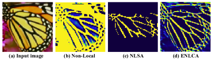
Figure 1: The visualization of correlation maps obtained by softmax and inner product between the marked red feature and all features. We can see that Non-Local attention pays attention to irrelevant features, and NLSA (Mei, Fan, and Zhou 2021) ignores the related features, while our ENLCA can simultaneously leverage relevant features and suppress irrelevant contents for SR.

Since SRCNN (Dong et al. 2015) firstly adopted deep learning in SISR, deep learning based methods have achieved a significant performance boost compared with traditional methods. The key to the success of deep learning is learnable feature representation. Therefore, certain works increase the depth and width of the network to further expand the receptive field and enhance representation ability. However, the solutions merely utilize relevant local information. Afterward, networks equip non-local modules, formulated as Eq 1, to exploit the image self-similarity prior globally and boost performance. Nevertheless, as shown in Figure 1 (b), the non-local module fuses excessive irrelevant features, which imports noise and limits the non-local module performance. In addition, the non-local module requires to compute feature mutual-similarity among all the pixel locations, which leads to quadratic computational cost to the input size. Limiting the non-local matching range can alleviate the issue at the expense of the loss of much global information. To address the problems, NLSA (Mei, Fan, and Zhou 2021) adopted Locality Sensitive Hashing (LSH) to aggregate the possible relevant features rapidly. However, as shown in Figure 1 (c), NLSA fixes the maximum number of hash buckets and chunk sizes to keep linear complexity with the input size, which results in ignoring important global related information.

In this paper, we aim to aggregate all important relevant features, keep the sparsity in the non-local module, and largely reduce its computational cost. Consequently, we propose a novel Efficient Non-Local Contrastive Attention (ENLCA) module and embed it into the deep SR network like EDSR. Specifically, we propose an Efficient Non-Local Attention (ENLA) module with kernel function approximation and associative law of matrix multiplication. The ENLA module achieves comparable performance as the standard non-local module while merely requiring linear computation and space complexity with respect to the input size. To further improve the performance of ENLA, we give the related features larger weights and ignore unrelated features in the aggregation process by multiplying the query and key by an amplification factor $k$. However, the kernel function of ENLA is based on Gaussian random vector approximation, and the variance of approximation increases exponentially with the inner product of query and key amplifying. Thus, we apply contrastive learning on ENLA to further increase the distance between relevant and irrelevant features. The contributions of our paper can be summarized as follows:

• We propose a novel Efficient Non-Local Contrastive Attention (ENLCA) for the SISR task. The ENLA of ENLCA significantly reduces the computational complexity from quadratic to linear by kernel function approximation and associative law of matrix multiplication.

• We enforce the aggregated feature sparsity by amplifying the query and key. In addition, we apply contrastive learning on the ENLA to further strengthen the effect of relevant features.

• A few ENLCA modules can improve a fairly simple ResNet backbone to state-of-the-arts. Extensive experiments demonstrate the advantages of ENLCA over the standard Non-Local Attention (NLA) and Non-Local Sparse Attention.

2 Related Work

2.1 Non-Local Attention in Super-Resolution

The SISR methods(Dong et al. 2015; Kim, Lee, and Lee 2016; Ledig et al. 2017; Wang et al. 2018) based on deep learning learn an end-to-end image mapping function between LR and HR images and obtain superior performance to conventional algorithms. In recent years, to further improve the performance of models, there is an emerging trend of applying non-local attention. Methods, such as CSNLN (Mei et al. 2020), SAN (Dai et al. 2019), RNAN (Zhang et al. 2019), NLRN (Liu et al. 2018), inserted non-local attention into their networks to make full use of recurring small patches and achieved considerable performance gain. However, the existing NLAs developed for SISR problems consume excessive computational resources and fuse much noisy information. Hence, NLSA (Mei, Fan, and Zhou 2021) uses Locality Sensitive Hashing (LSH) to efficiently aggregate several relevant features. Nevertheless, NLSA may miss the informative features, and computational cost can be further optimized. Motivated by recent work (Kitaev, Kaiser, and Levskaya 2020; Rahimi, Recht et al. 2007; Choromanski et al. 2020) on self-attention methods for natural language processing, we propose Efficient Non-Local Contrastive Attention (ENLCA) to learn global feature relations and reduce computational complexity.

2.2 Contrastive Learning

Contrastive learning has been widely studied for unsupervised representation learning in recent years. Instead of minimizing the difference between the output and a fixed target, contrastive learning (Chen et al. 2020; He et al. 2020; Henaff 2020; Oord, Li, and Vinyals 2018) maximizes the mutual information in representation space. Nevertheless, different from high-level vision tasks (Wu et al. 2018; He et al. 2020), there are few works to apply contrastive learning on low-level vision tasks. Recently, contrastive learning has been adopted in BlindSR(Zhang et al. 2021; Wang et al. 2021) to distinguish different degradations and achieved significant improvements. To the best of our knowledge, we are the first to introduce contrastive learning to the non-local module for enhancing sparsity by pulling relevant features close and pushing irrelevant away in representation space.

3 Efficient Non-Local Contrastive Attention

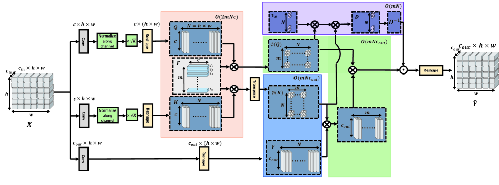
Figure 2: The illustration of Efficient Non-Local Attention. $h$ and $w$ are the input image height and width. $c_{in}$, $c$, and $c_{out}$ are the number of channels. $m$ indicates the number of random samples, and $N$ is the input size. $\boldsymbol{Q}$ and $\boldsymbol{K}$ are feature maps extracted from input $\boldsymbol{X}$. $\boldsymbol{F}$ is an Gaussian random matrix to transform $\boldsymbol{Q}$ and $\boldsymbol{K}$ to $\phi(\boldsymbol{Q})$ and $\phi(\boldsymbol{K})$, respectively. $\phi(\boldsymbol{Q})^{T}\phi(\boldsymbol{K})$ is the approximation of $exp(\boldsymbol{Q}^{T}\boldsymbol{K})$. $\boldsymbol{V}$ multiply $\phi(\boldsymbol{K})$ and $\phi(\boldsymbol{Q})$ successively to generate the features aggregating global information with linear computational complexity to the input size.

This section introduces the proposed Efficient Non-Local Contrastive Attention (ENLCA). The module realizes important global relevant information aggregation at the cost of linear complexity to the input size. Firstly, we develop Efficient Non-Local Attention (ENLA), the architecture of which is shown in Figure 2. Subsequently, as shown in Figure 4, we introduce Sparse Aggregation by multiplying the inputs an amplification factor and using contrastive learning for ENLCA to further filter noisy information. Finally, we utilize EDSR as the backbone to demonstrate the effectiveness of our module.

3.1 Efficient Non-Local Attention

Standard Non-Local Attention aggregates all features, which could propagate irrelevant noises into restored images. NLSA selects possible relevant features for aggregation by Locality Sensitive Hashing (LSH). However, LSH may ignore useful non-local information since it merely leverages relevant information roughly within limited window sizes. To alleviate the issue, we propose Efficient Non-Local Attention to aggregate all features efficiently.

Non-Local Attention. Non-local attention can explore self-exemplars by aggregating relevant features from the whole image. Formally, non-local attention is defined as:

$$\boldsymbol{Y}_{i}=\sum_{j=1}^{N}\frac{\exp\left(\boldsymbol{Q}_{i}^{T}\boldsymbol{K}_{j}\right)}{\sum_{\hat{j}=1}^{N}\exp\left(\boldsymbol{Q}_{i}^{T}\boldsymbol{K}_{\hat{j}}\right)}\boldsymbol{V}_{j},$$ (1)

$$\boldsymbol{Q}=\theta\left(\boldsymbol{X}\right),\boldsymbol{K}=\delta\left(\boldsymbol{X}\right),\boldsymbol{V}=\psi\left(\boldsymbol{X}\right),$$ (2)

where $\boldsymbol{Q}_{i},\boldsymbol{K}_{j}\in\mathbb{R}^{c}$ and $\boldsymbol{V}_{j}\in\mathbb{R}^{c_{out}}$ are pixel-wise features at location $i$ or $j$ on the feature map $\boldsymbol{Q}$, $\boldsymbol{K}$and $\boldsymbol{V}$ respectively. $\boldsymbol{Y}_{i}\in\mathbb{R}^{c_{out}}$ is the output at location $i$, $\boldsymbol{X}$ is the input and $N$ is the input size. $\theta(.)$, $\delta(.)$, and $\psi(.)$ are feature transformation functions for the input $\boldsymbol{X}$.

Efficient Non-Local Attention. The architecture of ENLA is shown in Figure 2. We decompose $\exp\left(\boldsymbol{Q}_{i}^{T}\boldsymbol{K}_{j}\right)$ by Gaussian random feature approximation and change multiplication order to obtain linear complexity with respect to image size. The decomposition of the exponential kernel function is derived as follows, and the detailed proofs are given in the supplementary.

$$\boldsymbol{Q}=\sqrt{k}\frac{\theta\left(\boldsymbol{X}\right)}{\|\theta\left(\boldsymbol{X}\right)\|},\boldsymbol{K}=\sqrt{k}\frac{\delta\left(\boldsymbol{X}\right)}{\|\theta\left(\boldsymbol{X}\right)\|},\boldsymbol{V}=\psi\left(\boldsymbol{X}\right),$$ (3)

$$\mathrm{K}(\boldsymbol{Q}_{i},\boldsymbol{K}_{j})=\exp\left(\boldsymbol{Q}_{i}^{\top}\boldsymbol{K}_{j}\right)$$ (4)

$$=\exp\left(-\left(\|\boldsymbol{Q}_{i}\|^{2}+\|\boldsymbol{K}_{j}\|^{2}\right)/2\right)\exp\left(\|\boldsymbol{Q}_{i}+\boldsymbol{K}_{j}\|^{2}/2\right)$$

$$=\mathbb{E}_{\boldsymbol{f}\sim\mathcal{N}\left(\boldsymbol{0}_{c},\boldsymbol{I}_{c}\right)}\exp\left(\boldsymbol{f}^{\top}\left(\boldsymbol{Q}_{i}+\boldsymbol{K}_{j}\right)-\frac{\|\boldsymbol{Q}_{i}\|^{2}+\|\boldsymbol{K}_{j}\|^{2}}{2}\right)$$

$$=\phi(\boldsymbol{Q}_{i})^{T}\phi(\boldsymbol{K}_{j}),$$

where $\boldsymbol{X}$ is the input feature map, and amplification factor $k$ $(k>1)$ is used for enforcing non-local sparsity. $\theta(.)$, $\delta(.)$, and $\psi(.)$ are feature transformation. $\boldsymbol{Q}_{i}$ and $\boldsymbol{K}_{j}\in\mathbb{R}^{c}$ are pixel-wise features at location $i$ or $j$ on the feature map $\boldsymbol{Q}$ and $\boldsymbol{K}\in\mathbb{R}^{c\times N}$. $\boldsymbol{f}\in\mathbb{R}^{c}$ and $\boldsymbol{f}\sim\mathcal{N}\left(\boldsymbol{0_{c}},\boldsymbol{I_{c}}\right)$. In practice, we set $m$ different Gaussian random samples $\boldsymbol{f}_{1},\ldots,\boldsymbol{f}_{m}\stackrel{{\scriptstyle\text{ iid }}}{{\sim}}\mathcal{N}\left(\boldsymbol{0}_{c},\boldsymbol{I}_{c}\right)$ and concatenate them as an Gaussian random matrix $\boldsymbol{F}\in\mathbb{R}^{m\times c}$. Consequently, the exponential-kernel admits a Gaussian random feature map unbiased approximation with $\phi(\boldsymbol{Q}_{i})^{T}\phi(\boldsymbol{K}_{j})$, where $\phi(\boldsymbol{u})=\frac{1}{\sqrt{m}}\exp\left(-\|\boldsymbol{u}\|^{2}/2\right)\exp\left(\boldsymbol{F}\boldsymbol{u}\right)$ for $\boldsymbol{u}\in\mathbb{R}^{c}$ and $\phi(\boldsymbol{u})\in\mathbb{R}^{m}$.

Based on the above deduction, the Efficient Non-Local Attention can be expressed as:

$$\boldsymbol{\hat{Y}}=\boldsymbol{D}^{-1}\left(\phi(\boldsymbol{Q})^{\top}\left(\phi(\boldsymbol{K})\boldsymbol{V}^{\top}\right)\right),$$ (5)

$$\boldsymbol{D}=\operatorname{diag}\left[\phi(\boldsymbol{Q})^{\top}\left(\phi(\boldsymbol{K})\boldsymbol{1}_{N}\right)\right],$$ (6)

where $\boldsymbol{\hat{Y}}$ stands for the approximated standard non-local attention, $\boldsymbol{D}$ is the normalization item in the softmax operator, and brackets indicate the order of computations.

We present here the theory analysis of variance of exponential kernel function approximation. The detailed proofs are given in the supplementary.

$$\operatorname{Var}\left(\phi(\boldsymbol{Q}_{i})^{T}\phi(\boldsymbol{K}_{j})\right)=$$ (7)

$$\frac{1}{m}\exp\left(-\left(\|\boldsymbol{Q}_{i}\|^{2}+\|\boldsymbol{K}_{j}\|^{2}\right)\right)\operatorname{Var}\left(\exp\left(\boldsymbol{f}^{\top}(\boldsymbol{Q}_{i}+\boldsymbol{K}_{j})\right)\right)$$

$$=\frac{1}{m}\mathrm{K}^{2}(\boldsymbol{Q}_{i},\boldsymbol{K}_{j})\left(\exp\left(\|\boldsymbol{Q}_{i}+\boldsymbol{K}_{j}\|^{2}\right)-1\right).$$

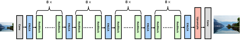
Figure 3: The proposed Efficient Non-Local Contrastive Network (ENLCN). Five ENLCA modules are embedded after every eight residual blocks.

Consequently, as $\mathrm{K}(\boldsymbol{Q}_{i},\boldsymbol{K}_{j})$ increases, the variance of $\phi(\boldsymbol{Q}_{i})^{T}\phi(\boldsymbol{K}_{j})$ increases exponentially. To guarantee the accuracy of the approximation results, multiplying $\mathrm{K}(\boldsymbol{Q}_{i},\boldsymbol{K}_{j})$ by a large amplification factor $k$ is impossible. Additionally, as (Choromanski, Rowland, and Weller 2017) did, keep Gaussian random samples orthogonal can reduce the approximation variance.

Computational Complexity. We analyze the computational complexity of the proposed ENLCA. As shown in Figure 2, the projections from $\boldsymbol{Q}$ and $\boldsymbol{K}$ to $\phi(\boldsymbol{Q})$ and $\phi(\boldsymbol{K})$ by matrix multiplication with $\boldsymbol{F}$ consume $\mathcal{O}(2mNc)$. The cost for the multiplication between $\phi(\boldsymbol{K})$ and $\boldsymbol{V}$ is $\mathcal{O}(mNc_{out})$. Similarly, the cost of the multiplication between $\phi(\boldsymbol{Q})$ and $\phi(\boldsymbol{K})\boldsymbol{V}^{\top}$ is $\mathcal{O}(mNc_{out})$ as well. Besides, the normalization item $\boldsymbol{D}$ adds additional $\mathcal{O}(mN)$. Therefore, the overall computational cost of our ENLCA is $\mathcal{O}(2mNc+2mNc_{out}+mN)$, which only takes linear computational complexity with respect to the input spatial size.

3.2 Sparse Aggregation

To further improve the performance of the Efficient Non-Local Attention, we filter out irrelevant information and enlarge the weight of related information.

Intuitively, multiplying the input by an amplification factor $k(k>1)$ enforces the non-local attention to give higher aggregation weight on related information, the essence of which is to enhance the sparsity of non-local attention weights. Unfortunately, multiplying an amplification factor $k(k>1)$ results in the increment of ENLA approximation variance.

To alleviate the problem, we further develop Efficient Non-Local Contrastive Attention (ENLCA) by applying contrastive learning. The goal of adopting contrastive learning is to increase the gap between irrelevant and relevant features. As shown in Figure 4, Contrastive Learning loss ${\cal L}_{cl}$ for training ENLCA can be formulated as:

$$\boldsymbol{T}_{i,j}=k\frac{\boldsymbol{Q}_{i}^{\top}}{\|\boldsymbol{Q}_{i}\|}\frac{\boldsymbol{K}_{j}}{\|\boldsymbol{K}_{j}\|},k>1,\boldsymbol{T}_{i,j}\in\boldsymbol{T},$$ (8)

$$\boldsymbol{T}_{i}^{\prime}=\operatorname{sort}\left(\boldsymbol{T}_{i},\operatorname{Descending}\right),\boldsymbol{T}_{i}^{\prime}\in\boldsymbol{T}^{\prime},\boldsymbol{T}_{i}\in\boldsymbol{T},$$ (9)

$${\cal L}_{cl}=\frac{1}{N}\sum_{i=1}^{N}-\log\frac{\sum_{j=1}^{n_{1}N}\exp\left(\boldsymbol{T}_{i,j}^{\prime}\right)/n_{1}N}{\sum_{j=n_{2}N}^{(n_{1}+n_{2})N}\exp\left(\boldsymbol{T}_{i,j}^{\prime}\right)/n_{1}N}+b,$$ (10)

where $N$ indicates the input size. $b$ is a margin constant. $n_{1}$ represents the percentage of relevant and irrelevant features in the feature map, and $n_{2}$ is the start index percentage for irrelevant features in the feature map, respectively. $\boldsymbol{T}_{i,j}$ measures relevance between $\boldsymbol{Q}_{i}$ and $\boldsymbol{K}_{j}$ by normalized inner product. $\boldsymbol{T}_{i}$ and $\boldsymbol{T}_{i}^{\prime}$ stand for $i$-th row of $\boldsymbol{T}$ and $\boldsymbol{T}^{\prime}\in\mathbb{R}^{N\times N}$ separately. Besides, $\boldsymbol{T}_{i}^{\prime}$ is descending sort result of $\boldsymbol{T}_{i}$.

Consequently, the overall loss function of our model is ultimately designed as:

$${\cal L}_{rec}=\left\|I^{HR}-I^{SR}\right\|_{1},$$ (11)

$${\cal L}={\cal L}_{rec}+\lambda_{cl}{\cal L}_{cl},$$ (12)

where ${\cal L}_{rec}$ is Mean Absolute Error (MAE) aiming to reduce distortion between the predicted SR image $I_{SR}$ and the target HR image $I_{HR}$, and the weight $\lambda_{cl}$ is 1e-3.

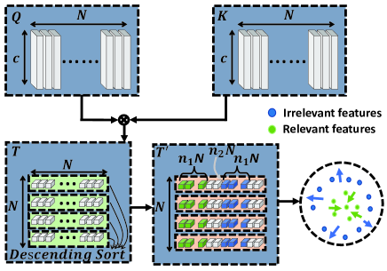
Figure 4: The illustration of our contrastive learning scheme for ENLCA. For each ordered sequence, we take the top $n_{1}N$ related ones as relevant features and $n_{1}N$ unrelated ones starting from $n_{2}N$ as irrelevant features.

3.3 Efficient Non-Local Contrastive Network

To demonstrate the effectiveness of our ENLCA module, we integrate it into the EDSR, a simple SR network consisting of 32 residual blocks, to form the Efficient Non-Local Contrastive Network (ENLCN). As shown in Figure 3, ENLCN uses five ENLCA modules with one insertion after every eight residual blocks.

Table 1: Quantitative results on benchmark datasets. Best and second best results are colored with red and blue.

Method	Scale	Set5	Set14	B100	Urban100	Manga109
		PSNR/SSIM	PSNR/SSIM	PSNR/SSIM	PSNR/SSIM	PSNR/SSIM
LapSRN	×2	37.52 / 0.9591	33.08 / 0.9130	31.08 / 0.8950	30.41 / 0.9101	37.27 / 0.9740
MemNet	×2	37.78 / 0.9597	33.28 / 0.9142	32.08 / 0.8978	31.31 / 0.9195	37.72 / 0.9740
SRMDNF	×2	37.79 / 0.9601	33.32 / 0.9159	32.05 / 0.8985	31.33 / 0.9204	38.07 / 0.9761
DBPN	×2	38.09 / 0.9600	33.85 / 0.9190	32.27 / 0.9000	32.55 / 0.9324	38.89 / 0.9775
RDN	×2	38.24 / 0.9614	34.01 / 0.9212	32.34 / 0.9017	32.89 / 0.9353	39.18 / 0.9780
RCAN	×2	38.27 / 0.9614	34.12 / 0.9216	32.41 / 0.9027	33.34 / 0.9384	39.44 / 0.9786
NLRN	×2	38.00 / 0.9603	33.46 / 0.9159	32.19 / 0.8992	31.81 / 0.9249	–
RNAN	×2	38.17 / 0.9611	33.87 / 0.9207	32.32 / 0.9014	32.73 / 0.9340	39.23 / 0.9785
SRFBN	×2	38.11 / 0.9609	33.82 / 0.9196	32.29 / 0.9010	32.62 / 0.9328	39.08 / 0.9779
OISR	×2	38.21 / 0.9612	33.94 / 0.9206	32.36 / 0.9019	33.03 / 0.9365	–
SAN	×2	38.31 / 0.9620	34.07 / 0.9213	32.42 / 0.9028	33.10 / 0.9370	39.32 / 0.9792
NLSN	×2	38.34 / 0.9617	34.08 / 0.9231	32.43 / 0.9027	33.42 / 0.9394	39.59 / 0.9789
EDSR	×2	38.11 / 0.9602	33.92 / 0.9195	32.32 / 0.9013	32.93 / 0.9351	39.10 / 0.9773
ENLCN (ours)	×2	38.37 / 0.9618	34.17 / 0.9229	32.49 / 0.9032	33.56 / 0.9398	39.64 / 0.9791
LapSRN	×4	31.54 / 0.8850	28.19 / 0.7720	27.32 / 0.7270	25.21 / 0.7560	29.09 / 0.8900
MemNet	×4	31.74 / 0.8893	28.26 / 0.7723	27.40 / 0.7281	25.50 / 0.7630	29.42 / 0.8942
SRMDNF	×4	31.96 / 0.8925	28.35 / 0.7787	27.49 / 0.7337	25.68 / 0.7731	30.09 / 0.9024
DBPN	×4	32.47 / 0.8980	28.82 / 0.7860	27.72 / 0.7400	26.38 / 0.7946	30.91 / 0.9137
RDN	×4	32.47 / 0.8990	28.81 / 0.7871	27.72 / 0.7419	26.61 / 0.8028	31.00 / 0.9151
RCAN	×4	32.63 / 0.9002	28.87 / 0.7889	27.77 / 0.7436	26.82 / 0.8087	31.22 / 0.9173
NLRN	×4	31.92 / 0.8916	28.36 / 0.7745	27.48 / 0.7306	25.79 / 0.7729	-
RNAN	×4	32.49 / 0.8982	28.83 / 0.7878	27.72 / 0.7421	26.61 / 0.8023	31.09 / 0.9149
SRFBN	×4	32.47 / 0.8983	28.81 / 0.7868	27.72 / 0.7409	26.60 / 0.8015	31.15 / 0.9160
OISR	×4	32.53 / 0.8992	28.86 / 0.7878	27.75 / 0.7428	26.79 / 0.8068	-
SAN	×4	32.64 / 0.9003	28.92 / 0.7888	27.78 / 0.7436	26.79 / 0.8068	31.18 / 0.9169
NLSN	×4	32.59 / 0.9000	28.87 / 0.7891	27.78 / 0.7444	26.96 / 0.8109	31.27 / 0.9184
EDSR	×4	32.46 / 0.8968	28.80 / 0.7876	27.71 / 0.7420	26.64 / 0.8033	31.02 / 0.9148
ENLCN (ours)	×4	32.67 / 0.9004	28.94 / 0.7892	27.82 / 0.7452	27.12 / 0.8141	31.33 / 0.9188

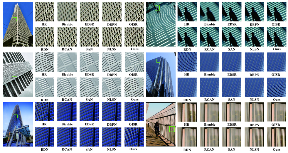
Figure 5: Visual comparison for $4\times$ SR on Urban100 dataset. For all the shown examples, our method significantly outperforms other state-of-the-arts, particularly in the image rich in repeated textures and structures.

4 Experiments

4.1 Datasets and Evaluation Metrics

Following EDSR (Lim et al. 2017) and RNAN (Zhang et al. 2019), we use DIV2K (Timofte et al. 2017), a dataset consists of 800 training images, to train our models. We test our method on 5 standard SISR benchmarks: Set5 (Bevilacqua et al. 2012), Set14 (Zeyde, Elad, and Protter 2010), B100 (Martin et al. 2001), Urban100 (Huang, Singh, and Ahuja 2015b) and Manga109 (Matsui et al. 2017). We evaluate all the SR results by PSNR and SSIM metrics on Y channel only in the transformed YCbCr space.

4.2 Implementation details

For ENLCA, we regenerate Gaussian random matrix $\boldsymbol{F}$ every epoch. Additionally, amplification factor $k$ is 6, and margin $b$ is 1. The number of random samples $m$ is set to 128. We build ENLCN using EDSR backbone with 32-residual blocks and 5 additional ENLCA blocks. All convolutional kernel size in the network is $3\times 3$. All intermediate features have 256 channels except for those embedded features in the attention module having 64 channels. The last convolution layer has 3 filters to transform the feature map into a 3-channel RGB image.

During training, we set $n_{1}$ and $n_{2}$ for contrastive learning to 2$\%$ and 8$\%$, separately. Besides, we randomly crop $28\times 28$ and $46\times 46$ patches from 16 images to form an input batch for $\times$4 and $\times$2 SR, respectively. We augment the training patches by randomly horizontal flipping and rotating $90^{\circ}$, $180^{\circ}$, $270^{\circ}$. The model is optimized by ADAM optimizer (Kingma and Ba 2014) with $\beta_{1}=0.9$, $\beta_{2}=0.99$ and initial learning rate of 1e-4. We reduce the learning rate by 0.5 after 200 epochs and obtain the final model after 1000 epochs. We first warm up the network via training 150 epochs with only ${\cal L}_{rec}$, then train with all loss functions. The model is implemented with PyTorch and trained on Nvidia 2080ti GPUs.

4.3 Comparisons with State-of-the-arts

To validate the effectiveness of our ENLCA, we compare our approach with 13 state-of-the-art methods, which are LapSRN (Lai et al. 2017), SRMDNF (Zhang, Zuo, and Zhang 2018), MemNet (Tai et al. 2017) , EDSR (Lim et al. 2017), DBPN (Haris, Shakhnarovich, and Ukita 2018), RDN (Zhang et al. 2018b), RCAN (Zhang et al. 2018a), NLRN (Liu et al. 2018), SRFBN (Li et al. 2019), OISR (He et al. 2019), SAN (Dai et al. 2019) and NLSN (Mei, Fan, and Zhou 2021).

In Table 1, we display the quantitative comparisons of scale factor $\times 2$ and $\times 4$. Compared with other methods, our ENLCN achieves the best results on almost all benchmarks and all scale factors. It is worth noting that adding additional ENLCAs brings significant improvement and even drives backbone EDSR outperforming the state-of-the-art methods, such as SAN and RCAN. Specifically, compared with EDSR, ENLCN improves about 0.2 dB in Set5, Set14, and B100 while around 0.5 dB in Urban100 and Manga109. Furthermore, compared with previous non-local based methods such as NLRN and RNAN, our network shows a huge superiority in performance. This is mainly because ENLCA only focuses on relevant features aggregation and filters out the noisy information from irrelevant features, which yields a more accurate prediction. Moreover, compared with the Sparse Non-Local Attention (NLSA) based method like NLSN, our ENLCN embodies advance in almost all entries. This is because NLSA aggregates relevant information roughly and may ignore important information, while ENLCA aggregates all relevant information. It is noted that all these improvements merely cost a small amount of computation, which roughly equals the computation of a convolution operation. The qualitative evaluations on Urban100 are shown in Figure 5.

5 Ablation Study

In this section, we conduct experiments to investigate our ENLCA. We build the baseline model with 32 residual blocks and insert corresponding attention variants after every 8 residual blocks.

Table 2: Ablation experiments conducted on Set5 ($\times$4) to study the effectiveness of the proposed Efficient Non-Local Attention (ENLA) module, multiplying amplification factor $k$, and contrastive learning.

Base	ENLA	$k$	contrastive learning	PSNR
✓	✗	✗	✗	32.21
✓	✓	✗	✗	32.37
✓	✓	✓	✗	32.44
✓	✓	✗	✓	32.41
✓	✓	✓	✓	32.48

Efficient Non-Local Contrastive Attention module. To demonstrate the effectiveness of the proposed Efficient Non-Local Contrastive Attention (ENLCA) module, we construct a baseline model by progressively adding our attention module or sparsity schemes. As shown in Table 2, comparing the first and the second row, Our ENLA brings 0.16 dB improvement over baseline, which demonstrates the effectiveness of ENLA. Furthermore, by solely adding the Sparsity Aggregation scheme such as multiplying the input by an amplification factor $k$ in Eq 3 and contrastive learning, results further improve around 0.07 dB. In the last row, we combine all modules and Sparsity Aggregation schemes, achieving an 0.27 dB improvement over the baseline.

These facts demonstrate that single Efficient Non-Local Attention (ENLA) works well in SISR. Besides, adding $k$ and contrastive learning to focus attention on the most informative positions is essential.

Table 3: The experiment conducted on Set5 ($\times$4) to explore the effects of $n_{1}(\%)$ and $n_{2}(\%)$ on contrastive learning.

	4	8	13	20
1	32.40	32.42	32.41	32.38
1.5	32.42	32.47	32.44	32.42
2	32.45	32.48	32.44	32.42
3	32.43	32.46	32.44	32.41

The effect of $n_{1}$ and $n_{2}$ on contrastive learning. The $n_{1}$ determines the percentage of relevant and irrelevant features participating in contrastive learning, and $n_{2}$ indicates the start index percentage of irrelevant features in the feature map. Results of the models trained on DIV2K ($\times$4, 200 epochs) and evaluated on Set5 ($\times$4) with different $n_{1}$ and $n_{2}$ are presented in Table 3. When $n_{1}=2\%$ and $n_{2}=8\%$, the model achieves the best performance. In the second column, with $n_{1}$ increase from 1$\%$ to 2$\%$, the PSNR improves for taking more informative features as relevant features and uninformative features as irrelevant features. However, as $n_{1}$ increases from 2$\%$ to 3$\%$, the performance decreases for fusing noisy features as relevant features. Similarly, in second rows, $n_{2}$ increases from 4$\%$ to 8$\%$ bringing improvements on the metric for taking less relative informative features as irrelevant features and increases from 8$\%$ to 20$\%$ leading to degradation of performance for missing taking noisy features as irrelevant features.

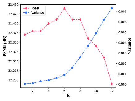
Figure 6: The relationship on amplification factor $k$ with SR results and approximation variance of ENLA.

The relationship on $k$ with SR results and approximation variance. We conduct the experiment on Set5 ($\times$4). As shown in Figure 6, when $k$ is set to 6, the model achieves the best performance. That is mainly because increasing $k$ causes the amplification of $\boldsymbol{Q}$ and $\boldsymbol{K}$, giving irrelevant features lower weight and relevant features larger weight in feature aggregation, but also results in the approximation variance of ENLA increasing exponentially. Hence, it is of crucial importance to find the right $k$ to balance the merits and demerits.

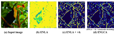
Figure 7: The verification of the sparsity bringing by Sparse Aggregation.

The effectiveness of Sparse Aggregation. To verify the sparsity bringing by Sparse Aggregation, we progressively add amplification factor $k$ and contrastive learning on ENLA and visualize the corresponding correlation maps obtained by softmax and inner product between the marked red feature and all features. As shown in Figure 7, ENLA gives large weights to unrelated regions. By multiplying the input by $k$, ENLA strengthens the effect of relevant features and suppresses irrelevant contents. When ENLA further adopts contrastive learning, the weights of relevant and irrelevant features are further distinct.

Table 4: Efficiency and performance comparison on Urban100 ($\times$4). $m$ is the number of random samples.

Methods	GFLOPs	PSNR
Baseline	0	26.64
NLA	25.60	26.87
Conv	0.74	-
NLSA-r4	5.08	26.96
ENLCA-$m$256	1.31	27.12
ENLCA-$m$128	0.66	27.12
ENLCA-$m$64	0.33	27.09
ENLCA-$m$32	0.16	27.07
ENLCA-$m$16	0.08	27.07
ENLCA-$m$8	0.04	27.03
ENLCA-$m$4	0.02	27.01
ENLCA-$m$2	0.01	26.88

Efficiency. We compare the proposed ENLCA with standard Non-Local Attention (NLA) in terms of computational efficiency. Table 4 shows the computational cost and the corresponding performances. The input is assumed to be the size of 100 $\times$ 100, and both input and output channels are 64. We also add a normal 3×3 convolution operation for better illustration. As shown in Table 4, ENLCA significantly reduces the computational cost of the NLA. Even compared with NLSA, our ENLCA achieves superior performance with much less computational cost. For example, our ENLCA-$m$16 brings 0.11 dB improvement on performance and is 100 times more efficient than NLSA. Furthermore, it is notable that our ENLCA has negligible computational cost compared with a convolution but achieves better performances than NLA and NLSA (Mei, Fan, and Zhou 2021). The best result is achieved by ENLCA-$m$128 and ENLCA-$m$256, which shows a bottleneck for increasing $m$ to improve performance.

6 Conclusion

In this paper, we propose a novel Efficient Non-Local Contrastive Attention (ENLCA) to enable effective and efficient long-range modeling for deep single image super-resolution networks. To reduce the excessive computational cost of non-local attention, we propose an Efficient Non-Local Attention (ENLA) by exploiting the kernel method to approximate exponential function. Furthermore, ENLCA adopts Sparse Aggregation, including multiplying inputs by an amplification factor and adding contrastive learning to focus on the most related locations and ignore unrelated regions. Extensive experiments on several benchmarks demonstrate the superiority of ENLCA, and comprehensive ablation analyses verify the effectiveness of ENLA and Sparse Aggregation.

7 Acknowledgments

This work was partly supported by the Natural Science Foundation of China (No.62171251), the Natural Science Foundation of Guangdong Province (No.2020A1515010711), the Special Foundation for the Development of Strategic Emerging Industries of Shenzhen (No.JCYJ20200109143010272) and Oversea Cooperation Foundation of Tsinghua Shenzhen International Graduate School.

Appendix A Appendix

A.1 Proof 1

In this section, we provide proof that our Efficient Non-Local Contrastive Attention (ENLCA) is the unbiased approximation of standard non-local attention.

First, we define $\boldsymbol{f}\in\mathbb{R}^{c}$ and use the fact that for any $\boldsymbol{Q}_{i},\boldsymbol{K}_{j},\in\mathbb{R}^{c}$,

$$(2\pi)^{-c/2}\int\exp\left(-\|\boldsymbol{f}-\left(\boldsymbol{Q}_{i}+\boldsymbol{K}_{j}\right)\|^{2}/2\right)d\boldsymbol{\boldsymbol{f}}=1.$$ (13)

Then, by using Eq.13, we can derive the approximation of $\exp\left(\|\boldsymbol{Q}_{i}+\boldsymbol{K}_{j}\|^{2}/2\right)$ as follows :

$$\exp\left(\|\boldsymbol{Q}_{i}+\boldsymbol{K}_{j}\|^{2}/2\right)=(2\pi)^{-c/2}\exp\left(\|\boldsymbol{Q}_{i}+\boldsymbol{K}_{j}\|^{2}/2\right)$$ (14)

$$\cdot\int\exp\left(-\|\boldsymbol{f}-(\boldsymbol{Q}_{i}+\boldsymbol{K}_{j})\|^{2}/2\right)d\boldsymbol{f}$$

$$=(2\pi)^{-c/2}\int\exp(-\|\boldsymbol{f}\|^{2}/2+\boldsymbol{f}^{\top}(\boldsymbol{Q}_{i}+\boldsymbol{K}_{j})$$

$$-\|\boldsymbol{Q}_{i}+\boldsymbol{K}_{j}\|^{2}/2+\|\boldsymbol{Q}_{i}+\boldsymbol{K}_{j}\|^{2}/2)d\boldsymbol{f}$$

$$=(2\pi)^{-c/2}\int\exp\left(-\|\boldsymbol{f}\|^{2}/2+\boldsymbol{f}^{\top}(\boldsymbol{Q}_{i}+\boldsymbol{K}_{j})\right)d\boldsymbol{f}$$

$$=(2\pi)^{-c/2}\int\exp\left(-\|\boldsymbol{f}\|^{2}/2\right)\cdot\exp\left(\boldsymbol{f}^{\top}(\boldsymbol{Q}_{i}+\boldsymbol{K}_{j})\right)d\boldsymbol{f}$$

$$=\mathbb{E}_{\boldsymbol{f}\sim\mathcal{N}\left(\boldsymbol{0}_{c},\boldsymbol{I}_{c}\right)}\left[\exp\left(\boldsymbol{f}^{\top}\left(\boldsymbol{Q}_{i}+\boldsymbol{K}_{j}\right)\right)\right].$$

By exploiting the approximation form in Eq.14 to obtain the unbiased approximation of $\exp\left(\boldsymbol{Q}_{i}^{\top}\boldsymbol{K}_{j}\right)$ as

$$\mathrm{K}(\boldsymbol{Q}_{i},\boldsymbol{K}_{j})=\exp\left(\boldsymbol{Q}_{i}^{\top}\boldsymbol{K}_{j}\right)$$ (15)

$$=\exp\left(-\left(\|\boldsymbol{Q}_{i}\|^{2}+\|\boldsymbol{K}_{j}\|^{2}\right)/2\right)\cdot\exp\left(\|\boldsymbol{Q}_{i}+\boldsymbol{K}_{j}\|^{2}/2\right)$$

$$=\mathbb{E}_{\boldsymbol{f}\sim\mathcal{N}\left(\boldsymbol{0}_{c},\boldsymbol{I}_{c}\right)}\exp\left(\boldsymbol{f}^{\top}\left(\boldsymbol{Q}_{i}+\boldsymbol{K}_{j}\right)-\frac{\|\boldsymbol{Q}_{i}\|^{2}+\|\boldsymbol{K}_{j}\|^{2}}{2}\right)$$

$$=\phi(\boldsymbol{Q}_{i})^{T}\phi(\boldsymbol{K}_{j}).$$

A.2 Proof 2

In this section, we provide the proof of approximation variance of ENLCA. Here, we denote: $\boldsymbol{z}=\boldsymbol{Q}_{i}+\boldsymbol{K}_{j}$.

From Eq.15, we can know that:

$$\mathbb{E}_{\boldsymbol{f}\sim\mathcal{N}\left(\boldsymbol{0}_{c},\mathbf{I}_{c}\right)}\left[\exp\left(\boldsymbol{f}^{\top}\boldsymbol{z}\right)\right]=\exp\left(\frac{\|\boldsymbol{z}\|^{2}}{2}\right).$$ (16)

From Eq.15, we can further derive the variance of approximation of $\exp\left(\boldsymbol{Q}_{i}^{\top}\boldsymbol{K}_{j}\right)$ as:

$$\operatorname{Var}\left(\phi(\boldsymbol{Q}_{i})^{T}\phi(\boldsymbol{K}_{j})\right)$$ (17)

$$=\frac{1}{m}\exp\left(-\left(\|\boldsymbol{Q}_{i}\|^{2}+\|\boldsymbol{K}_{j}\|^{2}\right)\right)\cdot\operatorname{Var}\left(\exp\left(\boldsymbol{f}^{\top}\boldsymbol{z}\right)\right)$$

$$=\frac{1}{m}\exp\left(-\left(\|\boldsymbol{Q}_{i}\|^{2}+\|\boldsymbol{K}_{j}\|^{2}\right)\right)$$

$$\cdot\left(\mathbb{E}\left[\exp\left(2\boldsymbol{f}^{\top}\boldsymbol{z}\right)\right]-\left(\mathbb{E}\left[\exp\left(\boldsymbol{f}^{\top}\boldsymbol{z}\right)\right]\right)^{2}\right)$$

$$=\frac{1}{m}\exp\left(-\left(\|\boldsymbol{Q}_{i}\|^{2}+\|\boldsymbol{K}_{j}\|^{2}\right)\right)$$

$$\cdot\left(\exp\left(2\|\boldsymbol{z}\|^{2}\right)-\exp\left(\|\boldsymbol{z}\|^{2}\right)\right)$$

$$=\frac{1}{m}\mathrm{K}^{2}(\boldsymbol{Q}_{i},\boldsymbol{K}_{j})\cdot\left(\exp\left(\|\boldsymbol{z}\|^{2}\right)-1\right)$$

$$=\frac{1}{m}\mathrm{K}^{2}(\boldsymbol{Q}_{i},\boldsymbol{K}_{j})\cdot\left(\exp\left(\|\boldsymbol{Q}_{i}+\boldsymbol{K}_{j}\|^{2}\right)-1\right).$$

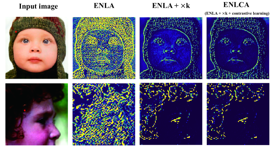
Figure 8: More visualization of the sparsity bringing by Sparse Aggregation. On the top of the ENLA module, multiplying the amplification factor $k$ ($\times k$) and contrastive learning are progressively added. The correlation maps are obtained by softmax and inner product between the marked red feature and all features.

A.3 Running Time Comparison

Here we present the running time comparison with standard Non-Local Attention (NLA) and Non-Local Sparse Attention (NLSA) (Mei, Fan, and Zhou 2021), following the settings in Table 4 of the paper. Models are evaluated at two input sizes: 100$\times$100 and 150$\times$150. We calculate the running time with the average of 1K times on one Nvidia 2080ti GPU. As shown in Table 5, compared with NLSA-r4 on the input with size of 150$\times$150, our ENLCA-m128 achieves around 0.2 dB improvement and significantly saves running time, demonstrating that ENLCA is indeed an efficient operation.

Table 5: Running time comparison with NLA and NLSA.

	100$\times$100 (ms)	150$\times$150 (ms)	PSNR (dB)
NLA	42.8	107.2	26.87
NLSA-r4	3.9	8.8	26.96
ENLCA-m128	0.9	1.6	27.12

A.4 Comparison with Criss-Cross Attention

Criss-Cross Attention is a variant of non-local attention widely used for high-level vision tasks. The Criss-Cross Attention aggregates the features on the criss-cross path of the query point to realize sparse aggregation. Thus, the aggregation features of Criss-Cross Attention merely depend on location. As shown in Table 6, ENLCA, NLSA and standard Non-Local Attention outperform Criss-Cross Attention. Besides, our ENLCA achieves the best performance. Compared with using sparsity in the fixed location, it is demonstrated that enforcing sparsity based on content relevance can better exploit the global relevant information.

Table 6: Comparison with Criss-Cross Attention on Urban100 ($\times 4$).

	baseline	Non-Local	Criss-Cross	NLSA	ENLCA
PSNR	26.64	26.87	26.85	26.96	27.12

A.5 More Visualization of Correlation Maps

In this paper, the proposed ENLCA consists of three major components: Efficient Non-Local Attention (ENLA) and Sparse Aggregation. The Sparse Aggregation includes Multiplying the input by an amplification factor $k$ ($\times k$) and contrastive learning. On the top of the ENLA, we progressively add the $\times k$ and contrastive learning. In Figure 8, we show more visualization of correlation maps to demonstrate the effectiveness of Sparse Aggregation.

References

- Bevilacqua et al. (2012) Bevilacqua, M.; Roumy, A.; Guillemot, C.; and line Alberi Morel, M. 2012. Low-Complexity Single-Image Super-Resolution based on Nonnegative Neighbor Embedding. In Proceedings of the British Machine Vision Conference, 135.1–135.10. BMVA Press. ISBN 1-901725-46-4.
- Chang, Yeung, and Xiong (2004) Chang, H.; Yeung, D.-Y.; and Xiong, Y. 2004. Super-resolution through neighbor embedding. In Proceedings of the 2004 IEEE Computer Society Conference on Computer Vision and Pattern Recognition, 2004. CVPR 2004., volume 1, I–I. IEEE.
- Chen et al. (2020) Chen, T.; Kornblith, S.; Norouzi, M.; and Hinton, G. 2020. A simple framework for contrastive learning of visual representations. In International conference on machine learning, 1597–1607. PMLR.
- Choromanski et al. (2020) Choromanski, K.; Likhosherstov, V.; Dohan, D.; Song, X.; Gane, A.; Sarlos, T.; Hawkins, P.; Davis, J.; Mohiuddin, A.; Kaiser, L.; et al. 2020. Rethinking attention with performers. arXiv preprint arXiv:2009.14794.
- Choromanski, Rowland, and Weller (2017) Choromanski, K.; Rowland, M.; and Weller, A. 2017. The unreasonable effectiveness of structured random orthogonal embeddings. arXiv preprint arXiv:1703.00864.
- Dai et al. (2007) Dai, S.; Han, M.; Xu, W.; Wu, Y.; and Gong, Y. 2007. Soft edge smoothness prior for alpha channel super resolution. In 2007 IEEE Conference on Computer Vision and Pattern Recognition, 1–8. IEEE.
- Dai et al. (2019) Dai, T.; Cai, J.; Zhang, Y.; Xia, S.-T.; and Zhang, L. 2019. Second-order attention network for single image super-resolution. In Proceedings of the IEEE/CVF Conference on Computer Vision and Pattern Recognition, 11065–11074.
- Dong et al. (2015) Dong, C.; Loy, C. C.; He, K.; and Tang, X. 2015. Image super-resolution using deep convolutional networks. IEEE transactions on pattern analysis and machine intelligence, 38(2): 295–307.
- Dong et al. (2012) Dong, W.; Zhang, L.; Shi, G.; and Li, X. 2012. Nonlocally centralized sparse representation for image restoration. IEEE transactions on Image Processing, 22(4): 1620–1630.
- Glasner, Bagon, and Irani (2009) Glasner, D.; Bagon, S.; and Irani, M. 2009. Super-resolution from a single image. In 2009 IEEE 12th international conference on computer vision, 349–356. IEEE.
- Haris, Shakhnarovich, and Ukita (2018) Haris, M.; Shakhnarovich, G.; and Ukita, N. 2018. Deep back-projection networks for super-resolution. In Proceedings of the IEEE conference on computer vision and pattern recognition, 1664–1673.
- He et al. (2020) He, K.; Fan, H.; Wu, Y.; Xie, S.; and Girshick, R. 2020. Momentum contrast for unsupervised visual representation learning. In Proceedings of the IEEE/CVF Conference on Computer Vision and Pattern Recognition, 9729–9738.
- He et al. (2019) He, X.; Mo, Z.; Wang, P.; Liu, Y.; Yang, M.; and Cheng, J. 2019. Ode-inspired network design for single image super-resolution. In Proceedings of the IEEE/CVF Conference on Computer Vision and Pattern Recognition, 1732–1741.
- Henaff (2020) Henaff, O. 2020. Data-efficient image recognition with contrastive predictive coding. In International Conference on Machine Learning, 4182–4192. PMLR.
- Huang, Singh, and Ahuja (2015a) Huang, J.-B.; Singh, A.; and Ahuja, N. 2015a. Single image super-resolution from transformed self-exemplars. In Proceedings of the IEEE conference on computer vision and pattern recognition, 5197–5206.
- Huang, Singh, and Ahuja (2015b) Huang, J.-B.; Singh, A.; and Ahuja, N. 2015b. Single image super-resolution from transformed self-exemplars. In Proceedings of the IEEE conference on computer vision and pattern recognition, 5197–5206.
- Kim, Lee, and Lee (2016) Kim, J.; Lee, J. K.; and Lee, K. M. 2016. Accurate image super-resolution using very deep convolutional networks. In Proceedings of the IEEE conference on computer vision and pattern recognition, 1646–1654.
- Kingma and Ba (2014) Kingma, D. P.; and Ba, J. 2014. Adam: A method for stochastic optimization. arXiv preprint arXiv:1412.6980.
- Kitaev, Kaiser, and Levskaya (2020) Kitaev, N.; Kaiser, Ł.; and Levskaya, A. 2020. Reformer: The efficient transformer. arXiv preprint arXiv:2001.04451.
- Lai et al. (2017) Lai, W.-S.; Huang, J.-B.; Ahuja, N.; and Yang, M.-H. 2017. Deep laplacian pyramid networks for fast and accurate super-resolution. In Proceedings of the IEEE conference on computer vision and pattern recognition, 624–632.
- Ledig et al. (2017) Ledig, C.; Theis, L.; Huszár, F.; Caballero, J.; Cunningham, A.; Acosta, A.; Aitken, A.; Tejani, A.; Totz, J.; Wang, Z.; et al. 2017. Photo-realistic single image super-resolution using a generative adversarial network. In Proceedings of the IEEE conference on computer vision and pattern recognition, 4681–4690.
- Li et al. (2019) Li, Z.; Yang, J.; Liu, Z.; Yang, X.; Jeon, G.; and Wu, W. 2019. Feedback network for image super-resolution. In Proceedings of the IEEE/CVF Conference on Computer Vision and Pattern Recognition, 3867–3876.
- Lim et al. (2017) Lim, B.; Son, S.; Kim, H.; Nah, S.; and Mu Lee, K. 2017. Enhanced deep residual networks for single image super-resolution. In Proceedings of the IEEE conference on computer vision and pattern recognition workshops, 136–144.
- Liu et al. (2018) Liu, D.; Wen, B.; Fan, Y.; Loy, C. C.; and Huang, T. S. 2018. Non-local recurrent network for image restoration. arXiv preprint arXiv:1806.02919.
- Martin et al. (2001) Martin, D.; Fowlkes, C.; Tal, D.; and Malik, J. 2001. A database of human segmented natural images and its application to evaluating segmentation algorithms and measuring ecological statistics. In Proceedings Eighth IEEE International Conference on Computer Vision. ICCV 2001, volume 2, 416–423. IEEE.
- Matsui et al. (2017) Matsui, Y.; Ito, K.; Aramaki, Y.; Fujimoto, A.; Ogawa, T.; Yamasaki, T.; and Aizawa, K. 2017. Sketch-based manga retrieval using manga109 dataset. Multimedia Tools and Applications, 76(20): 21811–21838.
- Mei, Fan, and Zhou (2021) Mei, Y.; Fan, Y.; and Zhou, Y. 2021. Image Super-Resolution With Non-Local Sparse Attention. In Proceedings of the IEEE/CVF Conference on Computer Vision and Pattern Recognition, 3517–3526.
- Mei et al. (2020) Mei, Y.; Fan, Y.; Zhou, Y.; Huang, L.; Huang, T. S.; and Shi, H. 2020. Image super-resolution with cross-scale non-local attention and exhaustive self-exemplars mining. In Proceedings of the IEEE/CVF Conference on Computer Vision and Pattern Recognition, 5690–5699.
- Oord, Li, and Vinyals (2018) Oord, A. v. d.; Li, Y.; and Vinyals, O. 2018. Representation learning with contrastive predictive coding. arXiv preprint arXiv:1807.03748.
- Rahimi, Recht et al. (2007) Rahimi, A.; Recht, B.; et al. 2007. Random Features for Large-Scale Kernel Machines. In NIPS, 5. Citeseer.
- Sun, Xu, and Shum (2008) Sun, J.; Xu, Z.; and Shum, H.-Y. 2008. Image super-resolution using gradient profile prior. In 2008 IEEE Conference on Computer Vision and Pattern Recognition, 1–8. IEEE.
- Tai et al. (2017) Tai, Y.; Yang, J.; Liu, X.; and Xu, C. 2017. Memnet: A persistent memory network for image restoration. In Proceedings of the IEEE international conference on computer vision, 4539–4547.
- Timofte et al. (2017) Timofte, R.; Agustsson, E.; Van Gool, L.; Yang, M.-H.; and Zhang, L. 2017. Ntire 2017 challenge on single image super-resolution: Methods and results. In Proceedings of the IEEE conference on computer vision and pattern recognition workshops, 114–125.
- Wang et al. (2021) Wang, L.; Wang, Y.; Dong, X.; Xu, Q.; Yang, J.; An, W.; and Guo, Y. 2021. Unsupervised Degradation Representation Learning for Blind Super-Resolution. In Proceedings of the IEEE/CVF Conference on Computer Vision and Pattern Recognition, 10581–10590.
- Wang et al. (2018) Wang, X.; Yu, K.; Wu, S.; Gu, J.; Liu, Y.; Dong, C.; Qiao, Y.; and Change Loy, C. 2018. Esrgan: Enhanced super-resolution generative adversarial networks. In Proceedings of the European Conference on Computer Vision (ECCV) Workshops, 0–0.
- Wu et al. (2018) Wu, Z.; Xiong, Y.; Yu, S. X.; and Lin, D. 2018. Unsupervised feature learning via non-parametric instance discrimination. In Proceedings of the IEEE conference on computer vision and pattern recognition, 3733–3742.
- Zeyde, Elad, and Protter (2010) Zeyde, R.; Elad, M.; and Protter, M. 2010. On single image scale-up using sparse-representations. In International conference on curves and surfaces, 711–730. Springer.
- Zhang et al. (2021) Zhang, J.; Lu, S.; Zhan, F.; and Yu, Y. 2021. Blind Image Super-Resolution via Contrastive Representation Learning. arXiv preprint arXiv:2107.00708.
- Zhang, Zuo, and Zhang (2018) Zhang, K.; Zuo, W.; and Zhang, L. 2018. Learning a single convolutional super-resolution network for multiple degradations. In Proceedings of the IEEE Conference on Computer Vision and Pattern Recognition, 3262–3271.
- Zhang et al. (2018a) Zhang, Y.; Li, K.; Li, K.; Wang, L.; Zhong, B.; and Fu, Y. 2018a. Image super-resolution using very deep residual channel attention networks. In Proceedings of the European conference on computer vision (ECCV), 286–301.
- Zhang et al. (2019) Zhang, Y.; Li, K.; Li, K.; Zhong, B.; and Fu, Y. 2019. Residual non-local attention networks for image restoration. arXiv preprint arXiv:1903.10082.
- Zhang et al. (2018b) Zhang, Y.; Tian, Y.; Kong, Y.; Zhong, B.; and Fu, Y. 2018b. Residual dense network for image super-resolution. In Proceedings of the IEEE conference on computer vision and pattern recognition, 2472–2481.
- Zontak and Irani (2011) Zontak, M.; and Irani, M. 2011. Internal statistics of a single natural image. In CVPR 2011, 977–984. IEEE.