A Low-Cost, Highly Customizable Solution for Position Estimation in Modular Robots

Abstract

Accurate position sensing is important for state estimation and control in robotics. Reliable and accurate position sensors are usually expensive and difficult to customize. Incorporating them into systems that have very tight volume constraints such as modular robots are particularly difficult. PaintPots are low-cost, reliable, and highly customizable position sensors, but their performance is highly dependent on the manufacturing and calibration process. This paper presents a Kalman filter with a simplified observation model developed to deal with the non-linearity issues that result in the use of low-cost microcontrollers. In addition, a complete solution for the use of PaintPots in a variety of sensing modalities including manufacturing, characterization, and estimation is presented for an example modular robot, SMORES-EP. This solution can be easily adapted to a wide range of applications.

$x$ or $\theta$Angular position $u$ or $\omega$Angular velocity of the driving motor(s) $V_{i}$Voltage measurement from wiper $i$ $\bar{\theta}_{i}$Shifted position measurement from wiper $i$ $k$Transmission ratio $n$Gaussian white noise in transition model $z$Measurement in Kalman filter $x^{i}$Reported state from the $i$th feature $z^{i}$Measurement from the $i$th feature $v^{i}$Observation noise of the $i$th feature $N(\bar{\mu},\bar{\Sigma})$Predicted Gaussian distribution of the angular position $N(\mu,\Sigma)$Updated Gaussian distribution of the angular position $K_{t}$Kalman gain at time $t$

1 Introduction

It is necessary to have accurate position sensing for most robotics control processes. Commercial position sensors are available for many applications. However, the form factor often presents a challenge to use these commercial off-the-shelf sensors. This is especially true for compact robotic systems with tight space constraints such as modular robotic systems [1]. Customizable position sensors give more flexibility to fit these situations.

Servos have been used in many modular robotic systems, such as Molecule [2] and CKBot [3]. Servo motors have built-in position control circuits. Some modular robotic systems, such as 3D Fracta [4], M-TRAN III [5], and SuperBot [6], use rotary potentiometers for position feedback. Optical or hall-effector sensor encoders are used in PolyBot [7], Crystalline [8], and ATRON [9] to report position information. These devices are usually too large for highly space-constrained systems, such as modular robots like SMORES-EP [10].

PaintPots are highly-customizable and low-cost position sensors that can be easily manufactured by widely accessible materials (spray paint and plastic sheets) and tools (laser cutters or scissors) [11]. The sensors can exist in different forms in terms of size, shape, and surface curvature. Thus, these sensors can be easily integrated with well designed parts or systems. The sensing performance and cost of PaintPot sensors make them competitive with commercial potentiometers [11] yet the customizability enable the use in situations which are not possible with commercial potentiometers.

Two different designs of PaintPot sensors are used in SMORES-EP modular robots. In each SMORES-EP module, there are four degrees of freedom (DOFs) requiring position sensing shown in Fig. 1 — three continuously rotating joints (LEFT DOF, RIGHT DOF, PAN DOF) and one bending joint with a $180\text{\,}\mathrm{\SIUnitSymbolDegree}$ range of motion (TILT DOF) [10]. Conductive spray paint is used to generate a resistive track surface. The manufacturing process is easy enough for a person to make a sensor quickly, but often does not yield consistent measurement and performance. The terminal-to-terminal resistance can vary over a large range depending on the thickness of the paint with a non-linear output. This fact complicates the position estimation for every DOF.

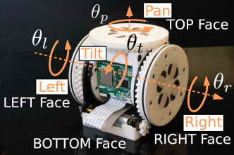
Figure 1: A SMORES-EP module has four degrees of freedom and four connectors.

For state estimation, stochastic techniques based on the probabilistic assumptions of the uncertainties in the system are widely applied. For linear systems, the Kalman filter [12] has been shown to be a reliable approach where uncertain parts in systems are assumed to have a particular probability distribution, usually Gaussian. Extensions including the extended Kalman filter (EKF) and unscented Kalman filter (UKF) [13] have been developed for nonlinear systems. For SMORES-EP DOF state estimation, we developed a new Kalman filter with a simpler observation model considering the non-linearity of PaintPot sensors. A complete and convenient calibration process is developed to precisely characterize each position sensor quickly. Four estimators can run on a $72\text{\,}\mathrm{MHz}$ microcontroller at the same time to track the states of all DOFs in a SMORES-EP module.

There are many applications that could use potentiometers but are too size constrained. For example goniometers in instrumented gloves for virtual reality currently use expensive strain gauge or non-linear flex sensing technologies. A joint angle potentiometer would be a good low-cost solution except for size constraints. Any compact device with a hinge (a flip phone, smart eyeglasses etc. or wearable devices) could have that joint angle measured to provide feedback. This paper presents an example solution of a class of potentiometers that is easily adapted to fit many low profile applications. It is semi-custom in that it is easily scalable to short-run numbers. These sensors are easily characterized and combined with our state estimation method, PaintPot sensors can provide reliable position information with little computation cost. Our solutions in SMORES-EP system shows that PaintPot sensors are promising for a variety of robotic applications.

The paper is organized as follows. Section 2 reviews relevant and previous work. Section 3 introduces the manufacturing and customized design for SMORES-EP system, as well as some necessary information. The characterization process is shown in Section 4 and the estimation method is presented in Section 5 for all DOFs. Some experiments are shown in Section 6. Finally, Section 7 talks about the conclusion.

2 Related Work

A potentiometer is a three-terminal resistor with a sliding or rotating contact (or wiper) that functions as a voltage divider [14]. There are three basic components in a potentiometer (Fig. 2): a resistive track, fixed electrical terminals on the track ends, and an electrical wiper. Different from most modern potentiometer tracks that are continuous semiconductive surfaces made of graphite, ceramic-metal composites (cermets), conductive plastics, or conductive polymer pastes, PaintPot sensors use an inexpensive carbon-embedded polymer spray paint [11].

Commercial vendors can customize potentiometers using industrial processes. For example, some manufacturers offer inkjet-printed thick-films that are deposited on printed circuit boards and other user specified surfaces and shapes for tracks. Two significant advantages of PaintPot solutions over these industrial processes are cost and time: compared with processes that often require thousands of dollars in up-front engineering fees, produce sensors that cost tens of dollars each, and have turnaround times of a week or more, PaintPot solutions can be used by a person or a team to create customized position sensors with the cost on the order of $1\text{\,}\mathrm{[}$$]USD per unit and also allows rapid iteration (limited only by the drying time of the paint).

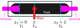
Figure 2: A Potentiometer has three terminals: two fixed electrical terminals at the resistive track ends and one electrical contact (wiper) that can move along the track surface.

Similar to PaintPot sensors, many rapid prototyping technologies allow electronics to be integrated into everyday objects at low cost. Self-folding printable resistors, capacitors, and inductors made of aluminum-coated polyester film (mylar) sheets are introduced in [15]. [16] presents a technique to accurately print low-resistance traces on sheet materials using silver nanoparticle ink deposited with a standard inkjet printer. PaintPot sensors can generate high resistance on order of $1\text{\,}\mathrm{k\SIUnitSymbolOhm}$ which is desirable for potentiometers used as voltage dividers.

This paper extends the conference version [11] on the same topic that includes the manufacturing process and performance of PaintPot sensors. PaintPot tracks are hand-painted using spray cans on $0.79\text{\,}\mathrm{m}\mathrm{m}$ thick plastic sheets. The sensors have good performance in terms of repeatability, resolution, and hysteresis compared with commercial potentiometers, but have a shorter lifetime. However, the performance of PaintPot sensors are highly dependent on the calibration process. This paper extends the conference version by presenting an integral and fast calibration process to characterize PaintPot sensors in SMORES-EP. Based on this, a new Kalman filter with a simplified observation model is developed to increase the reliability of these position sensors, especially for PaintPot sensors for continuously rotating joints where there are two coupled electric contacts, and the performance can be greatly improved compared with the simple rule presented in [11]. This reliable performance allows us to control a SMORES-EP chain to perform manipulation tasks [17].

3 PaintPot Sensor in SMORES-EP

PaintPots were originally developed to serve as position encoders for the SMORES-EP modular reconfigurable robot system [11]. Each SMORES-EP module (Fig. 1) is the size of an $80\text{\,}\mathrm{m}\mathrm{m}$ cube, and has an onboard battery, a microcontroller, and a Wi-Fi module to send and receive messages, as well as four actuated joints and electro-permanent magnet connectors on each face, allowing modules to connect to one another and self-reconfigure [18, 19]. The tight space requirements of SMORES-EP made it very difficult to incorporate off-the-shelf position encoders into the design, motivating the development of custom PaintPot encoders that occupy very little space within the robot. This section provides an overview of the manufacturing techniques used to create PaintPots, the fundamental material resolution of the sensors, and the design of the PaintPots used in SMORES-EP. For more detail, we refer the readers to [11].

3.1 Manufacturing Overview

The resistive track surface of a PaintPot encoder is made from conductive spray paint on a plastic track substrate. The PaintPots in SMORES-EP use three coats of MG Chemicals Total Ground conductive paint [20] sprayed onto Acrylonitrile butadiene styrene (ABS) plastic sheet. Three coats of paint are applied, with five minutes of drying time between coats, following the painting guidelines in the datasheet. ABS plastic can be cut to precise shapes in a laser cutter, and forms an ideal substrate for the paint, which readily bonds to the surface [20]. Electric terminals are created by mounting zinc-coated screws at the ends of the resistive strip. Applying paint above and beneath the screws creates an electrical connection between the track surface and the screw (Fig. 3). Leaded solder adheres to zinc-coated screws, allowing wires to be attached and detached.

Each PaintPot uses one or more wipers to measure the voltage at the point of contact with the resistive strip. Wipers with high contact pressure should be avoided, as they may scratch the paint. Larger contact surface area also reduces contact resistance, improving signal quality. The Harwin S1791-42 EMI Shield Finger Contact [21] is used in SMORES-EP. The wiper is a $4\text{\,}\mathrm{m}\mathrm{m}$ high gold-plated tin spring contact with a $1.45\text{\,}\mathrm{m}\mathrm{m}$$\times$$2.05\text{\,}\mathrm{m}\mathrm{m}$ contact area, and a contact force of $1\text{\,}\mathrm{N}$ (mounted on a PCB at a $3\text{\,}\mathrm{m}\mathrm{m}$ working height).

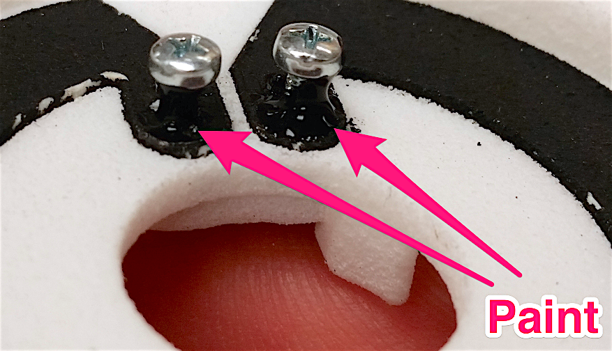
(a)

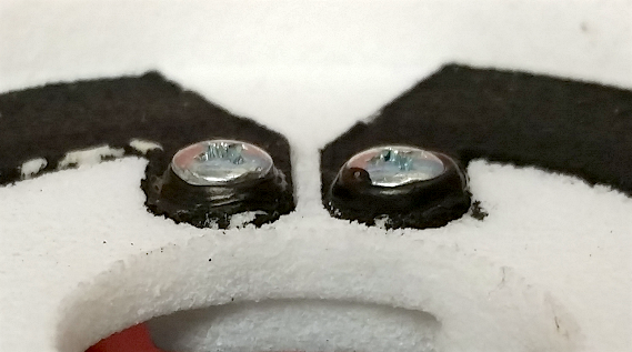
(b)

Figure 3: A bead of conductive paint applied beneath the screw head forms a good electrical connection with the track

3.2 Performance Characteristics

The fundamental material resolution of the resistive track was determined by characterizing the signal-to-noise ratio of the measured voltage on small length scales. Based on our experiments, the fundamental resolution of the track material is $8.63\pm$$0.126\text{\,}\mu\mathrm{m}$, which is of the same order of magnitude as some commercially available high-precision potentiometers. In SMORES-EP, the limiting factor in resolution is the analog-to-digital conversion bit depth ($10\text{\,}\mathrm{bit}$, or $84\text{\,}\mu\mathrm{m}$); to reach the material limit, $14\text{\,}\mathrm{bit}$ of analog-to-digital conversion depth would be required.

While PaintPots are not intended for long-lifetime applications, our analysis found that circular painted tracks have a lifetime of about 50,000 cycles when lubricated, which is sufficient for use in SMORES-EP.

3.3 Wheel and Tilt PaintPots in SMORES-EP

Each of the four articulated joints in SMORES-EP is equipped with a PaintPot, which provides absolute position encoding. The three continuously-rotating faces (labeled TOP, LEFT, and RIGHT in Fig. 1) have Wheel PaintPots with circular tracks and wipers offset parallel to the axis of rotation, while the central hinge has a Tilt PaintPot that covers $180\text{\,}\mathrm{\SIUnitSymbolDegree}$ arc with a wiper offset normal to the axis of rotation.

3.3.1 Wheel PaintPots

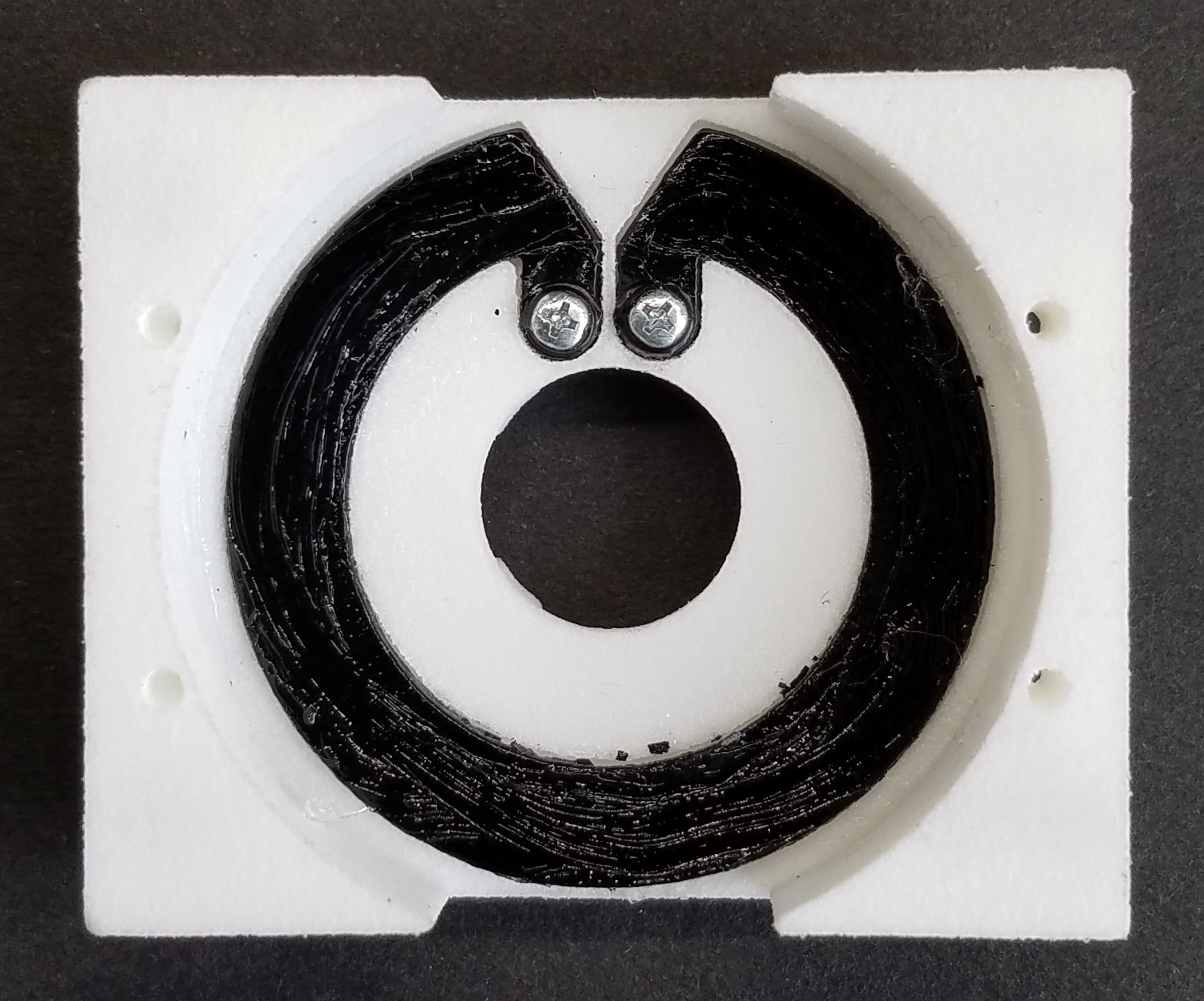
(a)

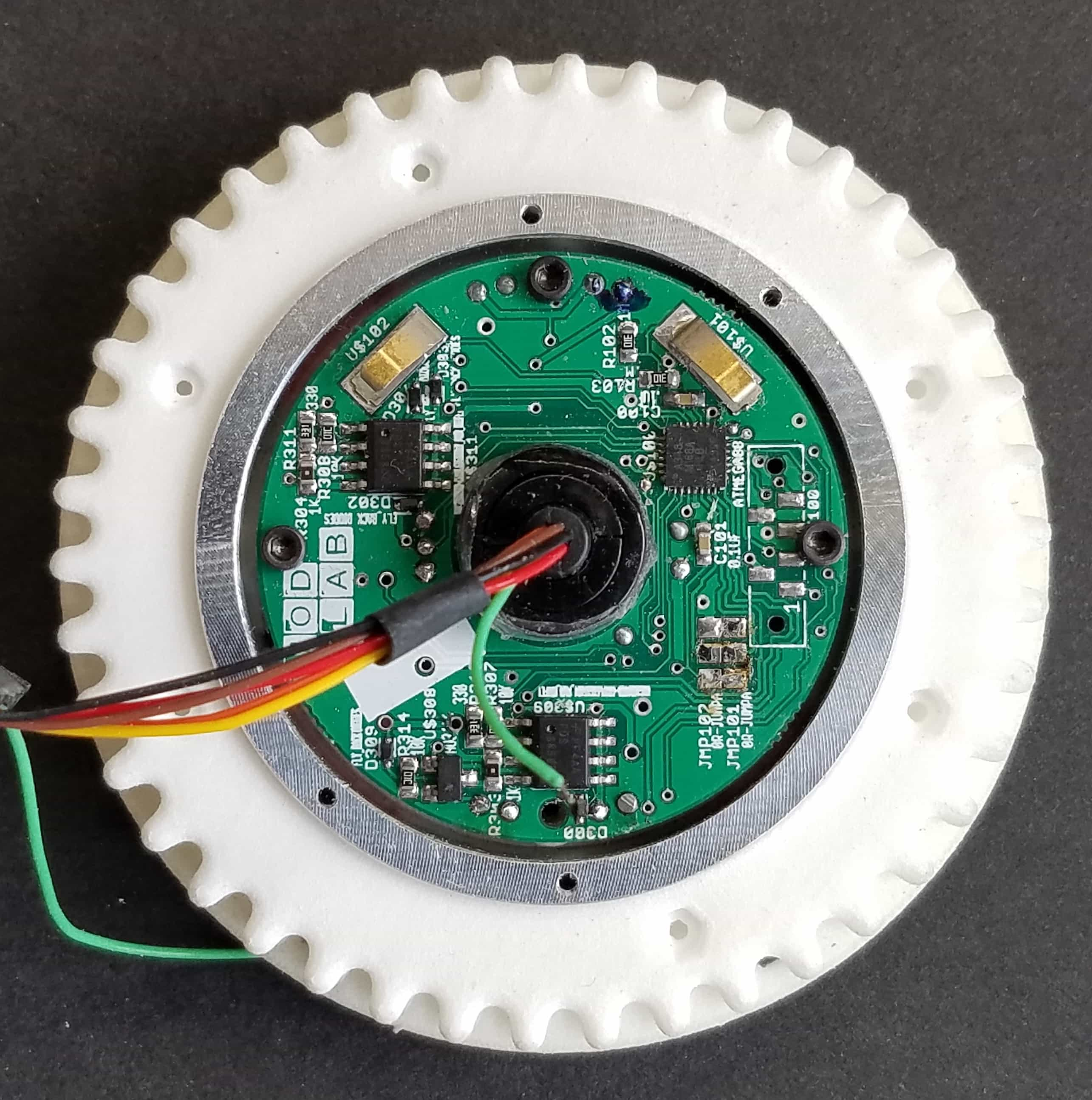
(b)

Figure 4: (a) A wheel PaintPot sensor is installed in a chassis. (b) Two wipers (Harwin S1791-42) are mounted on a circuit board at a $50\text{\,}\mathrm{\SIUnitSymbolDegree}$ angle to one another fixed to the wheel.

The wheel PaintPots, shown in Fig. 4a, have a circular track and two wiper contacts, allowing continuous rotation and providing position information over the full $360\text{\,}\mathrm{\SIUnitSymbolDegree}$ range of the left, right, and pan joints. The annular geometry allows a slip ring to fit through the center. Tabs on the track extend into the center of the circle to provide space for the terminal contacts. The V-shaped gap provides enough space for the wipers to pass from one side of the track to the other without contacting both simultaneously (which would cause a short circuit). The two wipers are mounted on a PCB above the track at a $50\text{\,}\mathrm{\SIUnitSymbolDegree}$ angle to one another (Fig. 4b); this configuration ensures that at least one wiper contacts the track at all times.

Tracks are cut in batches in a laser cutter. To facilitate easy mounting, a layer of double-sided adhesive is applied to the back of the ABS sheet before cutting. After cutting, three coats of paint are applied, and strips are allowed to dry for 24 hours. Strips are mounted in a mated groove in a 3D-printed chassis as shown in Fig. 4a. The chassis has a raised triangular feature that mates with the gap in the strip, so that the wipers remain at the same level as they pass through the gap region. Zinc-coated screws are used for electrical terminals. The measured terminal-to-terminal resistance of wheel PaintPots ranges from $2\text{\,}\mathrm{k\SIUnitSymbolOhm}$ to $20\text{\,}\mathrm{k\SIUnitSymbolOhm}$, depending on the thickness of the paint. Before use, a coat of petroleum-based grease is applied to the track surface.

3.3.2 Tilt PaintPots

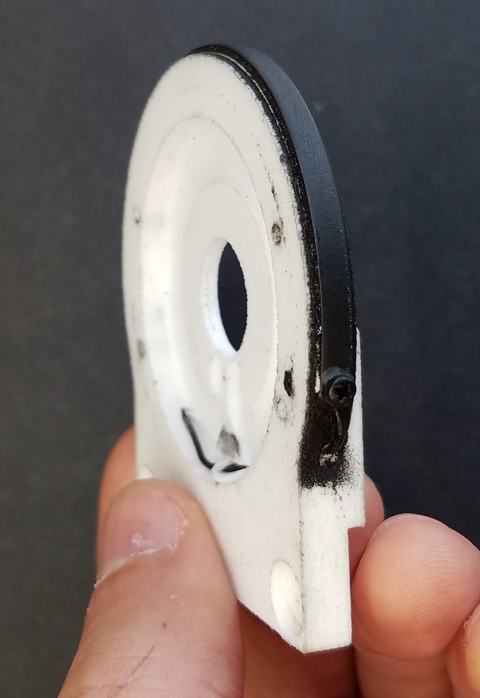
(a)

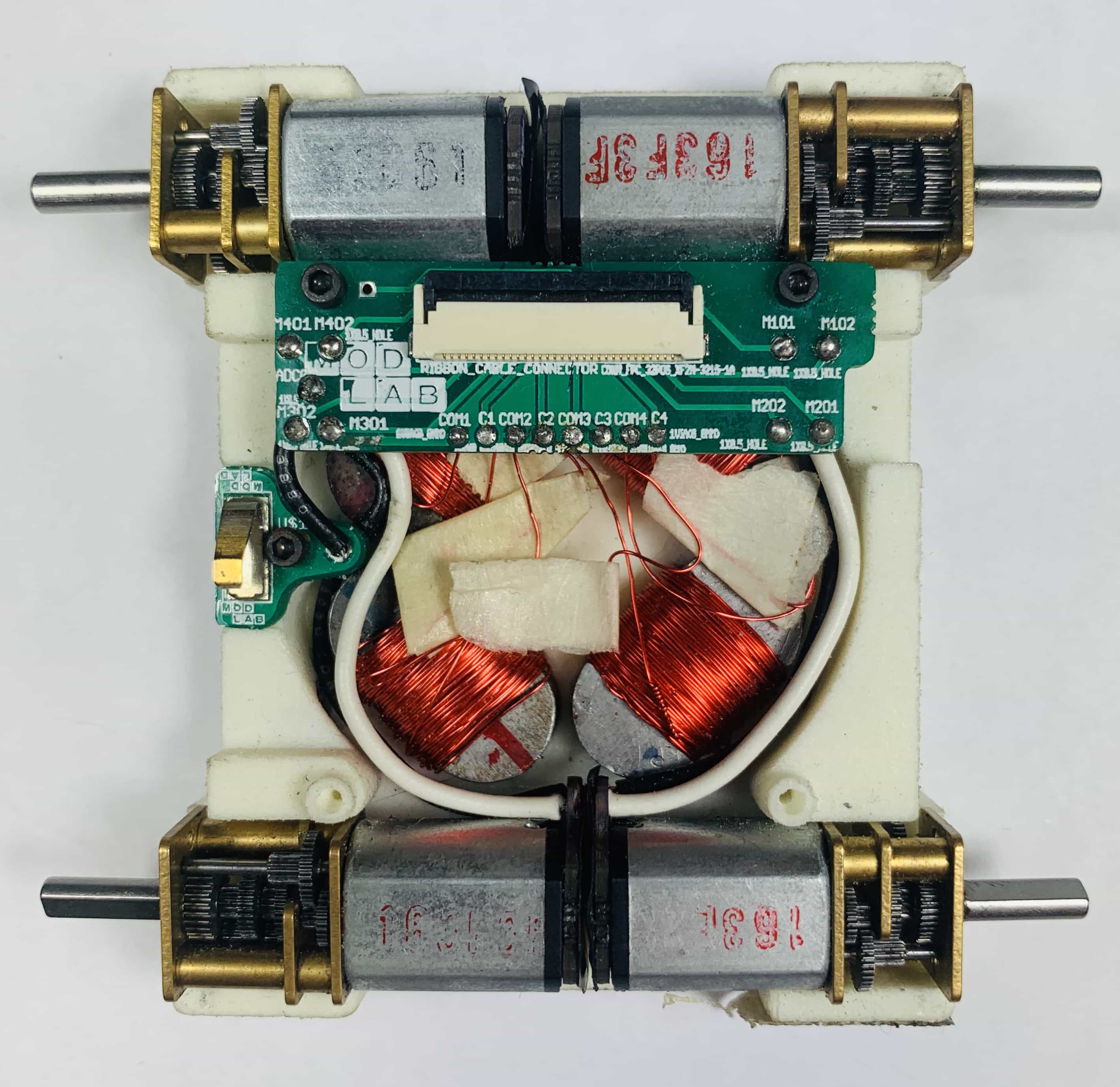
(b)

Figure 5: (a) A tilt PaintPot sensor is installed on a chassis. (b) A single wiper installed on the base of a SMORES-EP module contacts the track.

The tilt PaintPots, shown in Fig. 5a, have tracks with cylindrical curvature about their axis of rotation. A single wiper contacts the track and measures position through the full $180\text{\,}\mathrm{\SIUnitSymbolDegree}$ of motion of the tilt joint (Fig. 5b). The track geometry of the tilt PaintPot makes very efficient use of space inside the SMORES-EP module; to our knowledge, no off-the-shelf potentiometers replicate this unusual non-planar shape.

Tilt PaintPots have the same ABS/adhesive substrate as wheel PaintPots, and similar screw contacts. They are mounted to the 3D printed chassis before painting, allowing them to be painted in their final curved shape. This is preferable to painting flat and then bending: bending the paint after it has dried causes cracks to form, increases the resistance (three orders of magnitude), and causes a non-smooth variation of voltage along the length of the track. The terminal-to-terminal resistances of the tilt PaintPots range from $3\text{\,}\mathrm{k\SIUnitSymbolOhm}$ to $10\text{\,}\mathrm{k\SIUnitSymbolOhm}$.

3.4 Cost

The PaintPots used in SMORES-EP are inexpensive. The wipers are available from Digikey.com for $0.35\text{\,}\mathrm{[}$$]USD in quantities of 100. A $12\text{\,}\mathrm{o}\mathrm{z}$ MG Chemicals Total Ground spray paint can be purchased from Amazon.com for $16\text{\,}\mathrm{[}$$]USD, and $0.79\text{\,}\mathrm{m}\mathrm{m}$ ABS sheets can be purchased from McMaster.com for $3.70\text{\,}\mathrm{[}$$]USD per square foot. Based on these, materials for wheel PaintPots cost $1.05\text{\,}\mathrm{[}$$]USD and tilt PaintPots cost $0.70\text{\,}\mathrm{[}$$]USD. In order to build SMORES-EP modules with quality control testing [11], we yield about 75$\%$ of our wheel PaintPots and 90$\%$ of our tilt PaintPots, making the effective materials costs $1.40\text{\,}\mathrm{[}$$]USD and $0.78\text{\,}\mathrm{[}$$]USD respectively.

4 Sensor Characterization

Potentiometers used as voltage dividers typically model the input position as having linear relationship with the output voltage. Close adherence to the linear model has to be achieved by ensuring that the resistance between two points along the track is constant, which requires uniform geometry, thickness, and material properties of the track. This is difficult for PaintPots which are manually spray-painted. In order to obtain accurate position control on all DOFs of a SMORES-EP module, a calibration process is needed to characterize the performance of the particular PaintPots installed.

One terminal of a wheel PaintPot is connected with $3.3\text{\,}\mathrm{V}$ and the other terminal is connected with ground. Two wipers can contact the track and report current voltage ($V_{0}$ and $V_{1}$) in the form of two $10\text{\,}\mathrm{bit}$ analog-to-digital conversion values ranging from $01023$, and wheel position $\theta=$0\text{\,}\mathrm{rad}$$ is shown in Fig. 6 and the whole range of $\theta$ is from $-\pi\text{\,}\mathrm{rad}\pi\text{\,}\mathrm{rad}$. When a wiper contacts on or around the V-shape gap, the voltage value is not usable. This is the reason for having two wipers, to enable sensing the full $360\text{\,}\mathrm{\SIUnitSymbolDegree}$ range. So, $V_{0}$ should be ignored when $\theta$ is in the range from $\frac{2}{3}\pi\text{\,}\mathrm{rad}\frac{5}{6}\pi\text{\,}\mathrm{rad}$ and $V_{1}$ should be ignored when $\theta$ is in the range from $-\frac{5}{6}\pi\text{\,}\mathrm{rad}-\frac{2}{3}\pi\text{\,}\mathrm{rad}$.

Figure 6: When the wheel position $\theta=$0\text{\,}\mathrm{rad}$$, two wipers are contacting the track symmetrically to the middle location of it and $\theta$ ranges from $-\pi\text{\,}\mathrm{rad}\pi\text{\,}\mathrm{rad}$.

Figure 7: When the TILT DOF position $\theta=$0\text{\,}\mathrm{rad}$$, the wiper is contacting the middle of the track and $\theta$ ranges from $-\pi/2\text{\,}\mathrm{rad}\pi/2\text{\,}\mathrm{rad}$.

Similar to wheel PaintPots, the tilt PaintPot is also powered between ground and $3.3\text{\,}\mathrm{V}$ with one single wiper contacting the track all the times. The voltage $V_{0}$ from the voltage divider goes through a $10\text{\,}\mathrm{bit}$ analog-to-digital conversion (with range from $01023$). When the tilt position $\theta=$0\text{\,}\mathrm{rad}$$, the wiper is positioned in the middle of the track as shown in Fig. 7.

An automatic sensor calibration setup is developed based on AprilTags tracking [22] shown in Fig. 8a. Three tags are used to track the rigid bodies of a SMORES-EP module. Tag 2 is fixed to the base to be the reference frame, Tag 1 is fixed to the TOP Face of a SMORES-EP module for TILT DOF tracking, and Tag 0 can be fixed to LEFT Face, RIGHT Face, or TOP Face for wheel DOF tracking (Fig. 8b). During characterization, one DOF is moved at a time through its entire range of motion ($2\pi\text{\,}\mathrm{rad}$ for wheel DOF, $\pi\text{\,}\mathrm{rad}$ for TILT DOF) in both directions. The data, including $\theta$ and reported voltage, are recorded at $14\text{\,}\mathrm{H}\mathrm{z}$ (speed limited by the AprilTag ROS package).

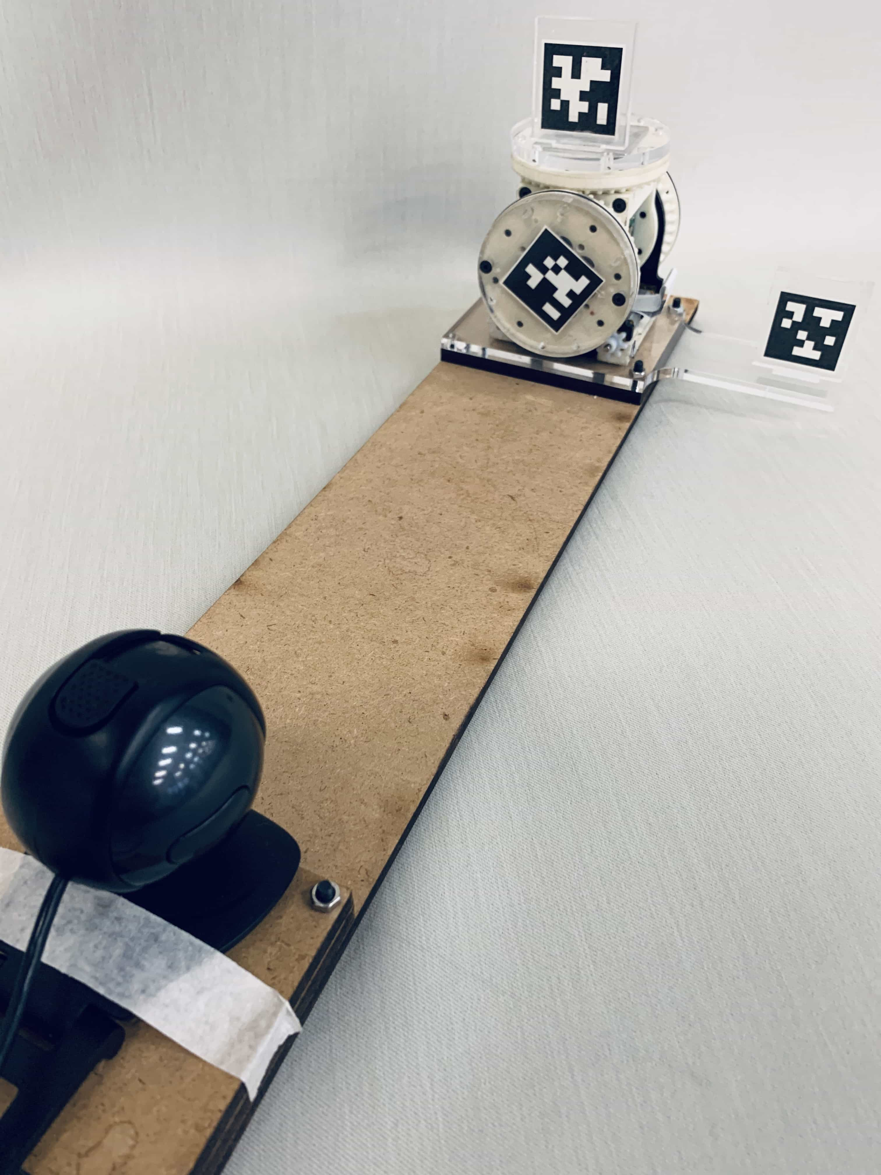
(a)

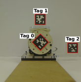
(b)

Figure 8: (a) Sensor characterization setup using AprilTags tracking approach. (b) Camera view of three tags in the characterization process.

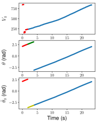
(a)

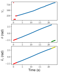
(b)

Figure 9: (a) Wiper 0 data through the entire range of a wheel PaintPot. (b) Wiper 1 data through the entire range of a wheel PaintPot.

While the voltage data is not linear with DOF position, it is monotonic (piece-wise monotonic for wheel DOFs). A third-order polynomial provides a suitable model. For a wheel PaintPot, the data from both wipers are shown in Fig. 9a and Fig. 9b respectively. For wiper 0, the reported voltage $V_{0}$ is not useful when DOF position $\theta$ is in the range from $\frac{2}{3}\pi\text{\,}\mathrm{rad}\frac{5}{6}\pi\text{\,}\mathrm{rad}$ (shown in red). Due to the gap of wheel PaintPots, $\theta=f_{0}(V_{0})$ is a piece-wise function which can be converted into a continuous function $\bar{\theta}_{0}=\bar{f}_{0}(V_{0})$ by shifting the segment ranging from $\frac{5}{6}\pi\text{\,}\mathrm{rad}\pi\text{\,}\mathrm{rad}$ (shown in green) by $2\pi\text{\,}\mathrm{rad}$ downward (shown in yellow). Similarly, for wiper 1, the segment when $\theta$ is in the range from $-\frac{5}{6}\pi\text{\,}\mathrm{rad}-\frac{2}{3}\pi\text{\,}\mathrm{rad}$ (shown in red) is meant to be trimmed, and the piece-wise function $\theta=f_{1}(V_{1})$ is converted into a continuous function $\bar{\theta}_{1}=\bar{f}_{1}(V_{1})$ by shifting the segment ranging from $-\pi\text{\,}\mathrm{rad}-\frac{5}{6}\pi\text{\,}\mathrm{rad}$ (shown in green) by $2\pi\text{\,}\mathrm{rad}$ upward (shown in yellow). After taking $50\text{\,}\mathrm{s}$ data in both directions (showing little hysteresis), $\bar{f}_{0}(V_{0})$ and $\bar{f}_{1}(V_{1})$ are shown in Fig. 10a and Fig. 10b respectively. An example run from a tilt PaintPot is shown in Fig. 11a and the characterization result $\theta=f(V_{0})$ is shown in Fig. 11b.

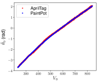
(a)

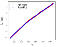
(b)

Figure 10: Wheel PaintPot sensor characterization results: (a) $\bar{\theta}_{0}=\bar{f}_{0}(V_{0})=$5.0281\text{\times}{10}^{-9}$V_{0}^{3}-$1.2255\text{\times}{10}^{-5}$V_{0}^{2}+$1.7856\text{\times}{10}^{-2}$V_{0}-7.2750$ and (b) $\bar{\theta}_{1}=\bar{f}_{1}(V_{1})=$5.1596\text{\times}{10}^{-9}$V_{1}^{3}-$1.2409\text{\times}{10}^{-5}$V_{1}^{2}+$1.7927\text{\times}{10}^{-2}$V_{1}-5.8128$.

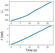
(a)

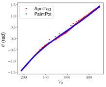
(b)

Figure 11: (a) Wiper data from $-80\text{\,}\mathrm{\SIUnitSymbolDegree}80\text{\,}\mathrm{\SIUnitSymbolDegree}$ of a tilt PaintPot. (b) The characterization result $\theta=f(V_{0})=$4.7517\text{\times}{10}^{-9}$V_{0}^{3}-$8.7608\text{\times}{10}^{-6}$V_{0}^{2}+$8.6756\text{\times}{10}^{-3}$V_{0}-2.7173$.

5 Position Estimation

5.1 Transition Model

Four DC motors are used to drive four DOFs (LEFT DOF, RIGHT DOF, PAN DOF, and TILT DOF) with a geared drive train shown in Fig. 12. The drive has pinion gears driving four identical spur gears. Two outer spur gears are attached to the left wheel and right wheel respectively for the LEFT DOF and RIGHT DOF. The crown gear is coupled to the two inner spur gears. When these two inner gears spin in the opposite direction, the top wheel attached to the crown gear rotates which is the PAN DOF. TILT DOF rotates when these two inner spur gears spin in the same direction. The transmission ratio for each DOF is determined by the gear train, then a linear relationship between the DOF velocity and the motor angular velocity can be obtained

$$\dot{\theta}=k\omega+n$$ (1)

in which $k$ is the transmission ratio of the DOF, $\omega$ is the angular velocity of the driving motor(s), $n\sim N(0,Q)$ is the additive Gaussian white noise, and $\dot{\theta}$ is the angular velocity of the DOF. The transition model of a DOF in discrete time can be derived by one-step Euler integration:

$$\theta_{t} =\theta_{t-1}+\dot{\theta}_{t-1}\delta t+n_{t-1}\delta t$$ (2)

$$=\theta_{t-1}+k\omega_{t-1}\delta t+n_{t-1}\delta t$$

$$=\theta_{t-1}+G\omega_{t-1}+Un_{t-1}$$

in which $\delta t$ is the finite time interval. Let $\theta$ be the state $x$ and $\omega$ be the system input $u$, then the transition model is

$$x_{t}=x_{t-1}+Gu_{t-1}+Un_{t-1}$$ (3)

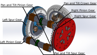
Figure 12: Four DOFs are driven by four actuators thorough a gear train.

5.2 Observation Model

In Section 4, a PaintPot can be characterized with a nonlinear model — a third-order polynomial $\theta=f(V)$. Here $V$ is the measurement, namely the reported voltage(s) from the wiper(s). Based on this, a nonlinear observation model $z=h(x)$ where $z$ is the measurement and $x$ is the state can be derived. We can linearize $z=h(x)$ about the current mean and variance of the DOF position $x$ to apply an extended Kalman filter (EKF). However, this places some computational burden on the SMORES-EP microcontroller. Here, we present a simple approach that can generate a linear observation model directly without linearization of the original nonlinear observation model about the current mean and variance of the state to overcome this nonlinearity. With this new approach, we just need to check if features are available using a simple rule and compute the new converted measurements by evaluating polynomials obtained from sensor characterization (Section 4).

5.2.1 Wheel PaintPots

For the wheel PaintPot sensor, the observation model is a piece-wise function due to the geometry of the sensor:

1. When $\theta\in($-\pi\text{\,}\mathrm{rad}$,$-\frac{5}{6}\pi\text{\,}\mathrm{rad}$)\cup($-\frac{2}{3}\pi\text{\,}\mathrm{rad}$,$\frac{2}{3}\pi\text{\,}\mathrm{rad}$)\cup($\frac{5}{6}\pi\text{\,}\mathrm{rad}$,$\pi\text{\,}\mathrm{rad}$)$, there are two valid measurements which are the reported voltages $V_{0}$ and $V_{1}$ from both wipers;

2. When $\theta\in\left[$-\frac{5}{6}\pi\text{\,}\mathrm{rad}$,$-\frac{2}{3}\pi\text{\,}\mathrm{rad}$\right]$, only $V_{1}$ is valid;

3. When $\theta\in\left[$\frac{2}{3}\pi\text{\,}\mathrm{rad}$,$\frac{5}{6}\pi\text{\,}\mathrm{rad}$\right]$, only $V_{0}$ is valid.

To accommodate the $2\pi\text{\,}\mathrm{rad}$ shift to obtain a continuous function for sensor characterization (Section 4), the observation can be modeled as

$$z=\begin{dcases}\left[\begin{matrix}V_{0}\\ V_{1}\end{matrix}\right]=\left[\begin{array}[]{c}\bar{f}_{0}^{-1}(x)\\ \bar{f}_{1}^{-1}(x+2\pi)\end{array}\right],&x<$-\frac{5}{6}\pi\text{\,}\mathrm{rad}$\\ V_{1}=\bar{f}^{-1}_{1}(x),&$-\frac{5}{6}\pi\text{\,}\mathrm{rad}$\leq x\leq$-\frac{2}{3}\pi\text{\,}\mathrm{rad}$\\ \left[\begin{matrix}V_{0}\\ V_{1}\end{matrix}\right]=\left[\begin{array}[]{c}\bar{f}_{0}^{-1}(x)\\ \bar{f}_{1}^{-1}(x)\end{array}\right],&$-\frac{2}{3}\pi\text{\,}\mathrm{rad}$<x<$\frac{2}{3}\pi\text{\,}\mathrm{rad}$\\ V_{0}=\bar{f}_{0}^{-1}(x),&$\frac{2}{3}\pi\text{\,}\mathrm{rad}$\leq x\leq$\frac{5}{6}\pi\text{\,}\mathrm{rad}$\\ \left[\begin{matrix}V_{0}\\ V_{1}\end{matrix}\right]=\left[\begin{array}[]{c}\bar{f}_{0}^{-1}(x-2\pi)\\ \bar{f}_{1}^{-1}(x)\end{array}\right],&x>$\frac{5}{6}\pi\text{\,}\mathrm{rad}$\end{dcases}$$ (4)

in which $x$ is the DOF position $\theta$.

In order to avoid linearizing this piece-wise observation model, we change the measurement to be the reported states rather than the two reported voltages. During the motion, there is at least one feature available for tracking, namely at least one wiper is contacting the wheel PaintPot at any time. Let $z^{i}$ be the measurement from the $i$th feature, then the measurement model with additive Gaussian white noise is simplified as

$$z^{i}=x^{i}+v^{i}=h^{i}(x,v^{i})\quad i=0,1$$ (5)

in which $v^{i}\sim N(0,R^{i})$, and $x^{i}$ is the reported state from $i$th feature determined by state $x$ in the following way:

$$x^{0}=\begin{dcases}x&x\leq\frac{5}{6}\pi\\ x-2\pi&x>\frac{5}{6}\pi\end{dcases}$$ (6a)

$$x^{1}=\begin{dcases}x+2\pi&x<-\frac{5}{6}\pi\\ x&x\geq-\frac{5}{6}\pi\end{dcases}$$ (6b)

Here, the measurement model is linear and the predicted measurement can be computed easily. The actual measurement for the $i$th feature can be obtained by evaluating $\bar{f}_{i}(V_{i})$ derived from the sensor characterization process. Recall that when $x\in\left[$\frac{2}{3}\pi\text{\,}\mathrm{rad}$,$\frac{5}{6}\pi\text{\,}\mathrm{rad}$\right]$, $V_{0}$ is not valid meaning this feature is not available. Otherwise the actual measurement from this feature is simply $\bar{f}_{0}(V_{0})$ if $x\notin\left[$\frac{2}{3}\pi\text{\,}\mathrm{rad}$,$\frac{5}{6}\pi\text{\,}\mathrm{rad}$\right]$. And the valid range of $V_{0}$ is from $V^{0}_{\min}=\bar{f}_{0}^{-1}(\frac{5}{6}\pi-2\pi)$ (because the segment from $\frac{5}{6}\pi\text{\,}\mathrm{rad}$ to $\pi\text{\,}\mathrm{rad}$ is shifted downward by $2\pi\text{\,}\mathrm{rad}$) to $V^{0}_{\max}=\bar{f}_{0}^{-1}(\frac{2}{3}\pi)$. Similar procedures can be applied to $V_{1}$, this feature is $\bar{f}_{1}(V_{1})$ if $x\notin\left[$-\frac{5}{6}\pi\text{\,}\mathrm{rad}$,$-\frac{2}{3}\pi\text{\,}\mathrm{rad}$\right]$, otherwise this feature is not available. The valid range of $V_{1}$ is from $V_{\min}^{1}=\bar{f}_{1}^{-1}(-\frac{2}{3}\pi)$ to $V_{\max}^{1}=\bar{f}_{1}^{-1}(-\frac{5}{6}\pi+2\pi)$.

5.2.2 Tilt PaintPots

The observation model for tilt PaintPots is straightforward which is

$$z=V_{0}=f^{-1}(x)$$ (7)

and it is a nonlinear function. Similarly, in order to avoid linearizing this observation model, we change the measurement to be the reported state and there is only one feature for tracking. Then the observation model with additive Gaussian white noise is simplified as

$$z=x+v=h(x,v)$$ (8)

in which $v\sim N(0,R)$ and the model is linear. The feature should always be available and the actual measurement for this feature is obtained by evaluating $f(V_{0})$.

5.3 Kalman Filter

With the transition model and the new form of observation model, a Kalman filter framework can be applied for state estimation.

5.3.1 Kalman Filter for Wheels

The initial state of a wheel DOF can be derived by any available feature. First check $V_{0}$, and if it is inside the valid range from $V_{\min}^{0}$ to $V_{\max}^{0}$, compute the initial state $x_{0}=\bar{f}_{0}(V_{0})$, and shift $x_{0}$ if necessary. That is if $x_{0}<-\pi$, let $x_{0}$ be $x_{0}+2\pi$. If $V_{0}\notin(V_{\min}^{0},V_{\max}^{0})$, then $x_{0}=\bar{f}_{1}(V_{1})$ because the wiper 1 must contact valid range of the track at this time, and similarly shift $x_{0}$ if necessary, namely if $x_{0}>\pi$, let $x_{0}$ be $x_{0}-2\pi$. The prior state can be represented as a Gaussian distribution $p(x_{0})\sim N(\mu_{0},\Sigma_{0})$ where $\mu_{0}=x_{0}$ and $\Sigma_{0}$ is initialized to an arbitrarily small value.

With Eq. (3), the prediction step is

$$\bar{\mu}_{t}=\mu_{t-1}+Gu_{t}$$ (9a)

$$\overline{\Sigma}_{t}=\Sigma_{t-1}+U^{2}Q$$ (9b)

With Eq. (5), Eq. (6a), and Eq. (6b), the predicted measurement $\bar{z}_{t}$ that is related to $x^{i}_{t}$ (the reported state from $i$th feature with $i=0,1$) can be computed. The analog-to-digital value $V_{i}$ from the $i$th feature at time $t$ is used to compute the actual measurement $z^{i}$. If $V_{i}\in(V^{i}_{\min},V^{i}_{\max})$, $z^{i}_{t}=\bar{f}_{i}(V_{i})$. Otherwise, this feature is not available. If both features are available, then $z_{t}=\left[z^{0}_{t},z^{1}_{t}\right]^{\intercal}$, $C_{t}=\left[1,1\right]^{\intercal}$, and the Kalman gain is

$$K_{t}=\overline{\Sigma}_{t}C_{t}^{\intercal}(C_{t}\overline{\Sigma}_{t}C_{t}^{\intercal}+R)^{-1}$$ (10)

in which $R=\mathrm{diag}(R^{0},R^{1})$. If there is only one feature (e.g. the $i$th feature) available, then $z_{t}=z^{i}_{t}$, $C_{t}=1$, and the Kalman gain is

$$K_{t}=\overline{\Sigma}_{t}C_{t}(C_{t}^{2}\overline{\Sigma}_{t}+R^{i})^{-1}$$ (11)

The state is then updated:

$$\mu_{t}=\bar{\mu}_{t}+K_{t}(z_{t}-\bar{z}_{t})$$ (12a)

$$\Sigma_{t}=\overline{\Sigma}_{t}-K_{t}C_{t}\overline{\Sigma}_{t}$$ (12b)

The estimated position for this wheel DOF at time $t$ is $\mu_{t}$.

5.3.2 Kalman Filter for Tilt

The initial state for a TILT DOF can be derived by evaluating $f(V_{0})$. The prior state can be represented as a Gaussian distribution $p(x_{0})\sim N(\mu_{0},\Sigma_{0})$ where $\mu_{0}=x_{0}$ and $\Sigma_{0}$ is initialized with some small value. The prediction step is in the same form with wheel DOFs (Eq. (9a) and Eq. (9b)). The predicted measurement can be computed from Eq. (8) which is simply $\bar{\mu}_{t}$. The current actual measurement is computed by evaluating $z_{t}=f(V_{0})$ where $V_{0}$ is the current reported voltage. Then the Kalman gain is simply

$$K_{t}=\overline{\Sigma}_{t}(\overline{\Sigma}_{t}+R)^{-1}$$ (13)

and the state is updated in the following:

$$\mu_{t}=\bar{\mu}_{t}+K_{t}(z_{t}-\bar{\mu}_{t})$$ (14a)

$$\Sigma_{t}=\overline{\Sigma}_{t}-K_{t}\overline{\Sigma}_{t}$$ (14b)

And the estimated position for TILT DOF at time $t$ is $\mu_{t}$.

6 Experiment

The PaintPot sensors, including wheel PaintPots and tilt PaintPots, are installed in SMORES-EP modules for position sensing. Currently, 25 SMORES-EP modules have been assembled. In the experiments, both a wheel PaintPot and a tilt PaintPot are characterized first and then the newly developed Kalman filters are implemented to show the effectiveness of our low-cost position sensing solution.

The data from both wipers for a wheel PaintPot is shown in Fig. 13a and Fig. 13b respectively. The segments labeled by red color are useless, and the green segments are shifted to the yellow segments to generate continuous functions to describe the relationship between voltage and angular position. This sensor is installed for PAN DOF on a SMORES-EP module. All our sensors are painted manually, so the quality is not consistent with no guarantees on bounds. The sensor characterization results for both wipers are shown in Fig. 14a and Fig. 14b respectively.

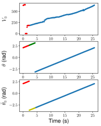
(a)

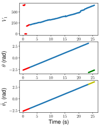
(b)

Figure 13: (a) Wiper 0 data through the entire range of a wheel PaintPot. (b) Wiper 1 data through the entire range of a wheel PaintPot.

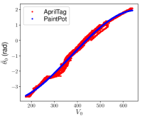
(a)

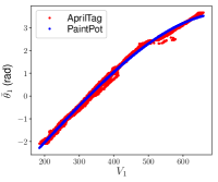
(b)

Figure 14: Wheel PaintPot sensor characterization results: (a) $\bar{\theta}_{0}=\bar{f}_{0}(V_{0})=$-6.5012\text{\times}{10}^{-8}$V_{0}^{3}+$7.2912\text{\times}{10}^{-5}$V_{0}^{2}-$1.1587\text{\times}{10}^{-2}$V_{0}-3.4595$ and (b) $\bar{\theta}_{1}=\bar{f}_{1}(V_{1})=$-1.8511\text{\times}{10}^{-8}$V_{1}^{3}+$1.0419\text{\times}{10}^{-5}$V_{1}^{2}+$1.4362\text{\times}{10}^{-2}$V_{1}-5.1767$.

With our Kalman filter, we are still able to derive good estimation of the angular position for the PAN DOF on this module. A simple controller is used to command the PAN DOF to a desired position from its current position along a fifth order polynomial trajectory. The first experiment commands the PAN DOF to angular position $0\text{\,}\mathrm{rad}$ from $\pi\text{\,}\mathrm{rad}$ resulting in an average error of $0.0878\text{\,}\mathrm{rad}$ as shown in Fig. 15a. In this experiment, $V_{0}$ is not valid for a while because wiper 0 contacts the gap of the track. The second experiment commands the PAN DOF to angular position $0\text{\,}\mathrm{rad}$ from $-\pi\text{\,}\mathrm{rad}$ with average error being $0.0698\text{\,}\mathrm{rad}$ as shown in Fig. 15b. In this experiment, $V_{1}$ is not valid when wiper 1 contacts the gap of the track.

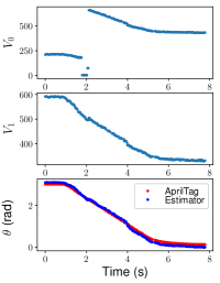
(a)

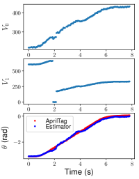
(b)

Figure 15: (a) Command PAN DOF to move from angular position $\pi\text{\,}\mathrm{rad}$ to $0\text{\,}\mathrm{rad}$. (b) Command PAN DOF to move from angular position $-\pi\text{\,}\mathrm{rad}$ to $0\text{\,}\mathrm{rad}$.

The data from the wiper for a tilt PaintPot is shown in Fig. 16a and the sensor characterization result is shown in Fig. 16b. In the experiment, this TILT DOF is commanded to traverse most of the range. The result from our estimator is shown in Fig. 17 with an average error being around $0.0325\text{\,}\mathrm{rad}$.

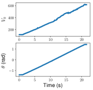
(a)

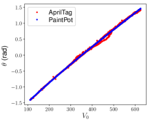
(b)

Figure 16: (a) Wiper data from $-80\text{\,}\mathrm{\SIUnitSymbolDegree}80\text{\,}\mathrm{\SIUnitSymbolDegree}$ of a tilt PaintPot. (b) The characterization result $\theta=f(V_{0})=$4.4674\text{\times}{10}^{-10}$V_{0}^{3}-$1.5933\text{\times}{10}^{-6}$V_{0}^{2}+$6.5369\text{\times}{10}^{-3}$V_{0}-2.1117$

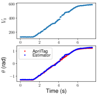
Figure 17: Command TILT DOF from angular position $-1.3\text{\,}\mathrm{rad}$ to $1.3\text{\,}\mathrm{rad}$.

7 Conclusion

In this paper, a complete low-cost and highly customizable position estimation solution is presented, especially suitable for highly space-constrained designs which is very common in modular robotic systems. PaintPots are low-cost, highly customizable, and can be manufactured easily by accessible materials and tools in low quantities. For the SMORES-EP system, two different types of PaintPot sensors are used, and a convenient automatic calibration approach is developed using AprilTags. A modified Kalman filter is developed to overcome the piece-wise nonlinearity of the sensors and some experiments show the accuracy. The successful application of PaintPots in SMORES-EP system shows that they can provide reliable position information with simple hardware setup. PaintPots can be easily adapted to and installed on a variety of systems, the not consistent performance due to the manufacturing process can be resolved by our characterization process which can be easily set up, and reliable state estimation can be derived by our modified Kalman filter that can be running on a low-cost microcontroller. The overall solution provides a new position sensing technique for a wide range of applications.

We would like to thank Hyun Kim for experiments and hardware maintenance. This work was funded in part by NSF grant number CNS-1329620.

References

- [1] Yim, M., Shen, W., Salemi, B., Rus, D., Moll, M., Lipson, H., Klavins, E., and Chirikjian, G., 2007. “Modular self-reconfigurable robot systems: Grand challenges of robotics”. IEEE Robotics & Automation Magazine, 14(1), pp. 43–52.
- [2] Castano, A., Behar, A., and Will, P. M., 2002. “The conro modules for reconfigurable robots”. IEEE/ASME Transactions on Mechatronics, 7(4), Dec, pp. 403–409.
- [3] Yim, M., White, P., Park, M., and Sastra, J., 2009. Modular Self-Reconfigurable Robots. Springer New York, New York, NY, pp. 5618–5631.
- [4] Murata, S., Kurokawa, H., Yoshida, E., Tomita, K., and Kokaji, S., 1998. “A 3-d self-reconfigurable structure”. In Proceedings. 1998 IEEE International Conference on Robotics and Automation (Cat. No.98CH36146), Vol. 1, pp. 432–439 vol.1.
- [5] Kurokawa, H., Tomita, K., Kamimura, A., Kokaji, S., Hasuo, T., and Murata, S., 2008. “Distributed self-reconfiguration of m-tran iii modular robotic system”. The International Journal of Robotics Research, 27(3-4), pp. 373–386.
- [6] Salemi, B., Moll, M., and Shen, W., 2006. “Superbot: A deployable, multi-functional, and modular self-reconfigurable robotic system”. In 2006 IEEE/RSJ International Conference on Intelligent Robots and Systems, pp. 3636–3641.
- [7] Yim, M., Duff, D. G., and Roufas, K. D., 2000. “Polybot: a modular reconfigurable robot”. In Proceedings 2000 ICRA. Millennium Conference. IEEE International Conference on Robotics and Automation. Symposia Proceedings (Cat. No.00CH37065), Vol. 1, pp. 514–520 vol.1.
- [8] Rus, D., and Vona, M., 2001. “Crystalline robots: Self-reconfiguration with compressible unit modules”. Autonomous Robots, 10(1), Jan, pp. 107–124.
- [9] Jorgensen, M. W., Ostergaard, E. H., and Lund, H. H., 2004. “Modular atron: modules for a self-reconfigurable robot”. In 2004 IEEE/RSJ International Conference on Intelligent Robots and Systems (IROS) (IEEE Cat. No.04CH37566), Vol. 2, pp. 2068–2073 vol.2.
- [10] Tosun, T., Davey, J., Liu, C., and Yim, M., 2016. “Design and characterization of the ep-face connector”. In 2016 IEEE/RSJ International Conference on Intelligent Robots and Systems (IROS), pp. 45–51.
- [11] Tosun, T., Edgar, D., Liu, C., Tsabedze, T., and Yim, M., 2017. “Paintpots: Low cost, accurate, highly customizable potentiometers for position sensing”. In 2017 IEEE International Conference on Robotics and Automation (ICRA), pp. 1212–1218.
- [12] Kalman, R. E., 1960. “A new approach to linear filtering and prediction problems”. Journal of Fluids Engineering, 82(1), 03, pp. 35–45.
- [13] Wan, E. A., and Van Der Merwe, R., 2000. “The unscented kalman filter for nonlinear estimation”. In Proceedings of the IEEE 2000 Adaptive Systems for Signal Processing, Communications, and Control Symposium (Cat. No.00EX373), pp. 153–158.
- [14] , 2000. “The authoritative dictionary of ieee standards terms, seventh edition”. IEEE Std 100-2000, Dec, pp. 1–1362.
- [15] Miyashita, S., Meeker, L., Go¨ldi, M., Kawahara, Y., and Rus, D., 2014. “Self-folding printable elastic electric devices: Resistor, capacitor, and inductor”. In 2014 IEEE International Conference on Robotics and Automation (ICRA), pp. 1446–1453.
- [16] Kawahara, Y., Hodges, S., Cook, B. S., Zhang, C., and Abowd, G. D., 2013. “Instant inkjet circuits: Lab-based inkjet printing to support rapid prototyping of ubicomp devices”. In Proceedings of the 2013 ACM International Joint Conference on Pervasive and Ubiquitous Computing, UbiComp ’13, ACM, pp. 363–372.
- [17] Liu, C., and Yim, M., 2020. “A quadratic programming approach to modular robot control and motion planning”. In 2020 Fourth IEEE International Conference on Robotic Computing (IRC), pp. 1–8.
- [18] Daudelin, J., Jing, G., Tosun, T., Yim, M., Kress-Gazit, H., and Campbell, M., 2018. “An integrated system for perception-driven autonomy with modular robots”. Science Robotics, 3(23), p. eaat4983.
- [19] Liu, C., Whitzer, M., and Yim, M., 2019. “A distributed reconfiguration planning algorithm for modular robots”. IEEE Robotics and Automation Letters, 4(4), Oct, pp. 4231–4238.
- [20] MG Chemicals, 2013. Total Ground Carbon Conductive Coating 838 Technical Data Sheet, January. Ver. 1.04.
- [21] Harwin Inc., 2016. S1791-42R Customer Information Sheet.
- [22] Olson, E., 2011. “Apriltag: A robust and flexible visual fiducial system”. In 2011 IEEE International Conference on Robotics and Automation, pp. 3400–3407.