Fitting AGN/galaxy X-ray-to-radio SEDs with CIGALE and improvement of the code

Abstract

Modern and future surveys effectively provide a panchromatic view for large numbers of extragalactic objects. Consistently modeling these multiwavelength survey data is a critical but challenging task for extragalactic studies. The Code Investigating GALaxy Emission (cigale) is an efficient python code for spectral energy distribution (SED) fitting of galaxies and active galactic nuclei (AGNs). Recently, a major extension of cigale (named x-cigale) has been developed to account for AGN/galaxy X-ray emission and improve AGN modeling at UV-to-IR wavelengths. Here, we apply x-cigale to different samples, including COSMOS spectroscopic type 2 AGNs, CDF-S X-ray detected normal galaxies, SDSS quasars, and COSMOS radio objects. From these tests, we identify several weaknesses of x-cigale and improve the code accordingly. These improvements are mainly related to AGN intrinsic X-ray anisotropy, X-ray binary emission, AGN accretion-disk SED shape, and AGN radio emission. These updates improve the fit quality and allow new interpretation of the results, based on which we discuss physical implications. For example, we find that AGN intrinsic X-ray anisotropy is moderate, and can be modeled as $L_{X}(\theta)\propto 1+\cos\theta$, where $\theta$ is the viewing angle measured from the AGN axis. We merge the new code into the major branch of cigale, and publicly release this new version as cigale v2022.0 on https://cigale.lam.fr

1 Introduction

Extragalactic surveys from X-ray to radio have become increasingly important for studying the evolution of galaxies and supermassive black holes (BHs) across cosmic history. Broad wavelength coverage provides insights into a diversity of properties of extragalactic sources. X-rays can reveal intrinsic active galactic nucleus (AGN) emission, even when it is obscured. UV/optical light traces young stars and unobscured AGN accretion disks. IR light reveals the dust-obscured AGN and/or star-formation (SF) activities. Radio emission can be generated by high-energy electrons associated with, e.g., AGN jets, AGN-driven winds, and HII regions.

Modern surveys such as LSST (Ivezić et al., 2019) and eRASS (Predehl et al., 2021) can sample millions-to-billions of diverse objects, from luminous quasars to low-luminosity AGNs, and from brightest cluster galaxies (BCGs) to dwarf galaxies. Interpreting these large volumes of multiwavelength data coherently and efficiently is a challenging task for extragalactic studies.

Many codes have been developed to fit AGN/galaxy spectral energy distributions (SEDs; see Fig. 1 of Thorne et al. 2020 for a summary of different codes). The Code Investigating GALaxy Emission (cigale) is an open-source SED-fitting code written in python (Burgarella et al., 2005; Boquien et al., 2019). It employs a parallel algorithm, able to build thousands of SED models per second and fit them to data. The SED models are built through a series of “modules” defined by the user. This architecture is designed to allow easy updates or even the addition of branches in the code that carries scientific investigations. For example, the dust-attenuation module applies a specific attenuation recipe to the starlight and line emission, and the dust-emission module is responsible for the IR dust radiation. The dust-emission module always normalizes the SED so that the re-emitted total energy is equal to the obscured total energy in the dust-attenuation module. In this way, cigale obeys the law of energy conservation. cigale has an AGN module that is responsible for the UV-to-IR emission from AGNs (Boquien et al., 2019; Ciesla et al., 2015).

Recently, Yang et al. (2020) developed a major cigale extension, x-cigale, adding a brand-new range of the electromagnetic spectrum (i.e., X-ray) to the existing UV-to-radio range. Yang et al. (2020) also implemented several AGN-related improvements including a clumpy torus model and a polar-dust model for x-cigale. The X-ray module allows the modeling of X-ray fluxes, accounting for the emission from both AGNs and galaxies (i.e., hot gas and X-ray binaries). x-cigale has become increasingly popular especially among AGN researchers (e.g., Zou et al., 2020; Mountrichas et al., 2021b; Ni et al., 2021; Toba et al., 2021; Yang et al., 2021).

In this work, we aim at testing x-cigale on diverse extragalactic populations, therefore we use several AGN/galaxy samples selected over different wavelength ranges, including COSMOS spectroscopic type 2 AGNs, CDF-S (Chandra Deep Field-South) X-ray detected normal galaxies, Sloan Digital Sky Survey (SDSS) quasars, and COSMOS radio objects. From these tests, we identify weaknesses and improve the code accordingly. These improvements are mainly related to AGN X-ray anisotropy, binary X-ray emission, AGN accretion-disk SED shape, and AGN radio emission. We discuss the physical implications based on the fitting results of the new code. Finally, we merge the new code into the main branch of cigale, after minimizing the differences between the two branches in terms of, e.g., coding structures and variable naming. This procedure removes a heavy burden of software maintenance, because, previously, an upgrade (such as algorithm improvements and additional functionalities) in cigale had to be modified and tested before implementation into x-cigale, and vice versa. We publicly release the merged software as cigale v2022.0 on the cigale official website, https://cigale.lam.fr

The structure of this paper is as follows. In §2, we fit a sample of type 2 AGNs and implement AGN anisotropic X-ray emission. In §3, we fit a sample of X-ray detected normal galaxies (non-AGNs) and introduce a flexible recipe for binary X-ray emission. In §4, we fit a sample of type 1 quasars and implement code changes allowing for more flexible AGN disk SED shapes. In §5, we fit a sample of radio sources and introduce an AGN radio component to the radio module. In §6, we present some miscellaneous updates of the code. We summarize our results and discuss future prospects in §7.

Throughout this paper, we assume a cosmology with $H_{0}=70$ km s^-1 Mpc^-1, $\Omega_{M}=0.3$, and $\Omega_{\Lambda}=0.7$. We adopt a Chabrier initial mass function (IMF; Chabrier 2003). Quoted uncertainties are at the $1\sigma$ (68%) confidence level. Quoted optical/infrared magnitudes are AB magnitudes. We adopt the “Bayesian-like” (rather than the best-fit) quantities in (x)-cigale output catalogs, unless otherwise stated. A Bayesian-like quantity/error are calculated as the average/standard deviation of all model values weighted by the probability distribution (Noll et al., 2009; Boquien et al., 2019).

2 AGN X-ray Anisotropy

2.1 Motivation

It is generally believed that the observed X-rays are a result of a “disk-corona” structure. The disk emits UV/optical photons, and a fraction of them are up-scattered to X-ray wavelengths by the high-energy electrons in the corona (i.e., inverse Compton scattering). The angular dependence of the X-ray emission is related to the detailed physical properties of the corona, such as shape and optical depth (e.g., Sunyaev & Titarchuk, 1985; Xu, 2015).

The observations of Liu et al. (2014) found that type 2 AGNs tend to systematically have lower intrinsic X-ray luminosity ($L_{\rm X}$) than type 1 AGNs at a given [o iv] 25.89 $\mu$m luminosity. Assuming that the [o iv] emission from the narrow-line region (NLR) is isotropic, they interpreted their result as an indicator of AGN X-ray anisotropy, because type 2 AGNs have larger viewing angles (as measured from the AGN axis) than type 1 AGNs under the scheme of AGN unification (e.g., Antonucci, 1993; Urry & Padovani, 1995; Netzer, 2015). Also, based on the X-ray and high-resolution mid-IR observations of nearby AGNs, Asmus et al. (2015) suggested that AGN X-ray emission might be anisotropic (see their section 5.4 for details).

However, x-cigale assumes that AGN intrinsic X-ray emission is isotropic, and does not allow anisotropic modeling. This assumption could overestimate the X-ray emission for type 2 viewing angles.

2.2 Sample and preliminary fitting

Table 1: Model parameters for the type 2 AGNs in COSMOS

Module	Parameter	Symbol	Values
Star formation history $\mathrm{SFR}\propto t\exp(-t/\tau)$	Stellar e-folding time	$\tau_{\rm star}$	0.1, 0.5, 1, 5 Gyr
	Stellar age	$t_{\rm star}$	0.5, 1, 3, 5, 7 Gyr
Simple stellar population Bruzual & Charlot (2003)	Initial mass function	$-$	Chabrier (2003)
	Metallicity	$Z$	0.02
Dust attenuation Calzetti et al. (2000)	Color excess	$E(B-V)$	0.05, 0.1, 0.2, 0.3, 0.4, 0.5, 0.7, 0.9 mag
Galactic dust emission: Dale et al. (2014)	Slope in $dM_{\rm dust}\propto U^{-\alpha}dU$	$\alpha$	2
AGN (UV-to-IR) SKIRTOR	AGN contribution to IR luminosity	${\rm frac_{AGN}}$	0–0.99 (step 0.1)
	Viewing angle	$\theta$	60, 70, 80, 90∘
	Polar-dust color excess	$E(B-V)_{\rm PD}$	0, 0.2, 0.4
X-ray	AGN photon index	$\Gamma$	1.8
	Maximum deviation from the $\alpha_{\rm ox}$-$L_{\nu,2500\textup{\AA}}$ relation	$|\Delta\alpha_{\rm ox}|_{\rm max}$	0.2
	AGN X-ray angle coefficients	$\boldsymbol{(a_{1},a_{2})}$	(0, 0) / (0.5, 0) / (1, 0) / (0.33, 0.67)a

Note. — For parameters not listed here, we use the default values. Bold font indicates new parameters in cigale v2022.0 introduced in this work. (a) Each set of angle coefficients is for one x-cigale run. $(a_{1},a_{2})=(0,0)$ indicates the x-cigale (isotropic) run.

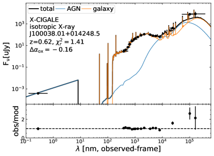
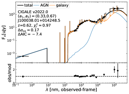
Figure 1: Example SED fits for a COSMOS type 2 AGNs from x-cigale (top-left panel) and cigale v2022.0 [three different $(a_{1},a_{2})$] as labeled. The cigale v2022.0 fits have better quality than the x-cigale fits, as indicated by the labeled $\Delta\rm AIC$ values (see §2.4 for the $\Delta\rm AIC$ definition). Therefore, the X-ray anisotropic models are preferred over the isotropic one for this example source.

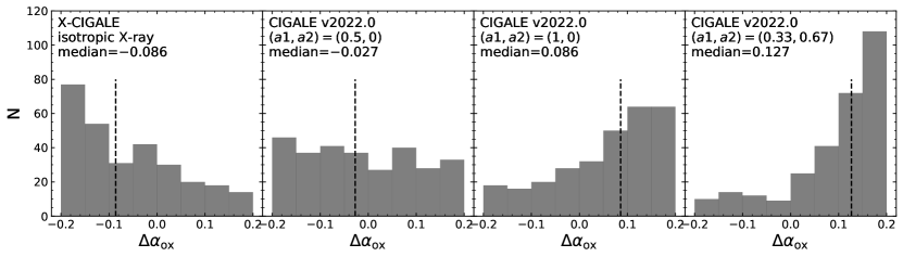
Figure 2: $\Delta\alpha_{\rm ox}$ distributions for COSMOS type 2 AGNs from x-cigale and cigale v2022.0 [three different $(a_{1},a_{2})$] as labeled. We use the best-fit $\Delta\alpha_{\rm ox}$ values here, because x-cigale cannot perform Bayesian-like analysis for the quantity of $\Delta\alpha_{\rm ox}$ due to a technical reason. The vertical dashed line indicates the median value of each distribution. These median values are also labeled on each panel. The new x-cigale fits with $(a_{1},a_{2})=(0.5,0)$ have median $\Delta\alpha_{\rm ox}$ closest to zero, indicating that this anisotropy model is the most physical among the four models (one isotropic and three anisotropic) tested.

In x-cigale, the AGN X-ray emission is modeled using the $\alpha_{\rm ox}$-$L_{\nu,2500\textup{\AA}}$ relation from Just et al. (2007), where $L_{\nu,2500\textup{\AA}}$ is the intrinsic disk emission at a viewing angle of 30^∘ and $\alpha_{\rm ox}$ is the AGN SED slope connecting $L_{\nu,2500\textup{\AA}}$ and $L_{\rm\nu,2keV}$. For type 1 AGNs, whose viewing angles are near 30^∘ (Yang et al., 2020), the SEDs are similar for isotropic and anisotropic X-ray models in the framework of x-cigale. However, for type 2 AGNs, whose viewing angles are much larger than 30^∘, the isotropic and anisotropic models will predict significantly different X-ray emissions, at a given AGN power.

To test the effectiveness of x-cigale (isotropic X-ray emission), we use a spectroscopic type 2 AGN sample from the Chandra COSMOS-Legacy survey (Civano et al. 2016; Marchesi et al. 2016). We require these AGNs to have $S/N>3$ in the hard band of Chandra (2–7 keV), and we apply absorption corrections to the hard-band fluxes based on the correction factors from Marchesi et al. (2016), because x-cigale requires that the input X-ray fluxes are intrinsic (Yang et al., 2020). The absorption corrections from Marchesi et al. (2016) are based on a standard hardness-ratio analyses.

We remove sources with $L_{\rm X}<10^{42.5}$ erg s^-1, for which the X-ray emission might originate from normal galaxies rather than AGNs (e.g., Aird et al., 2017). We adopt the 14 broad-band photometric data ($u$ to IRAC 8 $\mu$m) from the COSMOS2015 catalog (Laigle et al., 2016). We also use the MIPS 24 $\mu$m, PACS 100/160 $\mu$m, and SPIRE 250/350/500 $\mu$m photometry from the “super-deblended” catalog of Jin et al. (2018). There are a total of 296 type 2 AGNs, spanning a redshift range of 0.3–1.6 (10%–90% percentile).

Our fitting parameters are listed in Table 1. For the star formation history (SFH), we adopt a delayed $\tau$ SFH model and a Bruzual & Charlot (2003) simple stellar population model. We adopt the Calzetti et al. (2000) galaxy attenuation law and the Dale et al. (2014) dust IR spectral templates. For AGN IR emission, we adopt the SKIRTOR clumpy torus model (Stalevski et al., 2012, 2016). We fix the torus half opening angle to the default 40^∘, which is observationally preferred (e.g., Stalevski et al., 2016). Under this setting, there are four type-2 viewing angles (60, 70, 80, and 90^∘) available in SKIRTOR, and we allow all these values in our fits (see Table 1). The full SKIRTOR model set has another five parameters such as 9.7 $\mu$m optical depth and ratio of outer to inner radius. These parameters generally have minor effects on the broad-band SED shapes (e.g., Yang et al. 2020), and thus we leave them at the default values to reduce the needed computing resources. In summary, we employ four templates (corresponding to different viewing angles) out of the total 19200 SKIRTOR models. In x-cigale, AGN X-ray and UV/optical emissions are related with the $\alpha_{\rm ox}$-$L_{\nu,2500\textup{\AA}}$ relation of Just et al. (2007), where $\alpha_{\rm ox}$ is the UV/X-ray slope calculated at the typical AGN type-1 viewing angle of $\theta=30^{\circ}$ (Yang et al., 2020), i.e.,

$$\alpha_{\rm ox}=-0.3838\log\frac{L_{\nu,2500\textup{\AA}}(30^{\circ})}{L_{\rm\nu,2keV}(30^{\circ})},$$ (1)

where $L_{\nu,2500\textup{\AA}}$ and $L_{\rm\nu,2keV}$ are the monochromatic AGN luminosities per frequency at rest-frame 2500 $\rm\AA$ and 2 keV, respectively. Although the $\alpha_{\rm ox}$-$L_{\nu,2500\textup{\AA}}$ relation is reasonably tight, it has a non-negligible intrinsic scatter of $\approx 0.1$ in terms of $\alpha_{\rm ox}$ (e.g., Steffen et al., 2006; Just et al., 2007). x-cigale considers the scatter by constructing different models around the $\alpha_{\rm ox}$-$L_{\nu,2500\textup{\AA}}$ relation, and the user can set the maximum deviation from the relation, $|\Delta\alpha_{\rm ox}|_{\rm max}$ (see §2.2.3 of Yang et al. 2020 for details). In our fits, we set $|\Delta\alpha_{\rm ox}|_{\rm max}=0.2$ (Table 1), about $2\sigma$ of the intrinsic scatter (e.g., Just et al., 2007). We set the photon index $\Gamma=1.8$, a typical value for distant X-ray AGNs (e.g., Yang et al., 2016; Liu et al., 2017).

Fig. 1 (top-left) shows an example SED fit for one of the COSMOS type 2 AGNs. Under the scheme of AGN unification (e.g., Antonucci, 1993; Urry & Padovani, 1995; Netzer, 2015), our type 2 AGNs should also follow the $\alpha_{\rm ox}$-$L_{\nu,2500\textup{\AA}}$ intrinsic relation (Eq. 1). To test this point, we plot the $\Delta\alpha_{\rm ox}=\alpha_{\rm ox,fitted}-\alpha_{\rm ox,expected}$ (i.e., deviation from the $\alpha_{\rm ox}$-$L_{\nu,2500\textup{\AA}}$ relation) distribution from our x-cigale run in Fig. 2. The $\Delta\alpha_{\rm ox}$ values tend to be systematically negative, with a median value of $-0.093$ (corresponding to a factor of 1.75 lower in terms of $L_{\rm\nu,2keV}/L_{\nu,2500\textup{\AA}}$) for x-cigale. This result suggests that, with the assumption of isotropic AGN X-ray emission in x-cigale, the observed X-ray fluxes of our type 2 AGNs tend to systematically lie below the expectations from the $\alpha_{\rm ox}$-$L_{\nu,2500\textup{\AA}}$ relation. One natural solution to this issue is allowing intrinsic X-ray anisotropy, so that an AGN viewed at type 2 angles will have lower X-ray fluxes than viewed at type 1 angles. We perform this code-implementation task in §2.3.

2.3 Code Improvement

Considering the evidence for X-ray anisotropy in §2.1 and §2.2, we modify the code so that the user can model $L_{\rm X}$ as a 2nd-order polynomial function of the cosine of the viewing angle (e.g., Netzer, 1987):

$$\frac{L_{\rm X}(\theta)}{L_{\rm X}(0)}=a_{1}\cos\theta+a_{2}\cos^{2}\theta+1-a_{1}-a_{2},$$ (2)

where the coefficients ($a_{1}$ and $a_{2}$) are free parameters set by the user and $\theta$ is the viewing angle (face-on $=0$, edge-on $=90^{\circ}$). The constant term in Eq. 2, $1-a_{1}-a_{2}$, guarantees that the right-hand side equals the left-hand side when $\theta=0$. Setting $(a_{1},a_{2})=(0,0)$ mean isotropic $L_{\rm X}$. In cigale v2022.0, $\alpha_{\rm ox}$ is still calculated using Eq. 1.

2.4 Results and interpretation

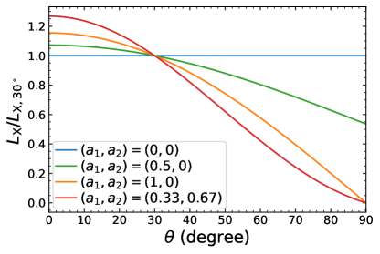
Figure 3: Dependence of $L_{\rm X}$ on viewing angle. Different colors indicate different $(a_{1},a_{2})$ settings that are tested in this work. $(a_{1},a_{2})=(0,0)$ indicates the x-cigale (isotropic) test. The $L_{\rm X}$ ($y$-axis) is normalized at $\theta=30^{\circ}$, where the $\alpha_{\rm ox}$-$L_{\nu,2500\textup{\AA}}$ relation is applied in x-cigale and cigale v2022.0.

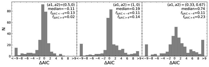
Figure 4: Distribution of AIC difference between the fits of cigale v2022.0 and x-cigale. Different panels are for the fits with different $(a_{1},a_{2})$ values as labeled. The median value and the fractions of $\Delta\rm AIC<-4$ and $\Delta\rm AIC>4$ are marked on each panel. The new x-cigale fits with $(a_{1},a_{2})=(0.5,0)$ has overall the best fit quality compared to other ones.

We repeat the fitting of type 2 AGNs (§2.1) but using cigale v2022.0. We perform three runs each with ($a_{1}$, $a_{2}$) set to $(0.5,0)$, $(1,0)$, and $(0.33,0.67)$, respectively, while other parameters are the same as the run in §2.2 (see Table 1). $(a_{1},a_{2})=(0.33,0.67)$ means the same angular dependence as that of the AGN disk emission ($L_{\rm disk}$) in the UV-to-IR AGN module (the SKIRTOR model; Stalevski et al. 2012, 2016). $(a_{1},a_{2})=(1,0)$ is equivalent to a thin disk geometry with an angle-independent X-ray intensity. The angle dependence of $(a_{1},a_{2})=(0.5,0)$ is between $(a_{1},a_{2})=(1,0)$ and the isotropic case. Fig. 3 displays the viewing angular dependence under these ($a_{1}$, $a_{2}$) settings. The angular dependence is stronger in the order of $(0.5,0)$, $(1,0)$, and $(0.33,0.67)$.

The SED fit for an example source is displayed in Fig. 1. For this source, the anisotropic models have better fitting quality than the isotropic model (as indicated by the reduced $\chi^{2}$ labeled in Fig. 1). Fig. 2 displays the $\Delta\alpha_{\rm ox}$ distributions from the cigale v2022.0 runs. The settings of $(a_{1},a_{2})=(1,0)$ and $(a_{1},a_{2})=(0.33,0.67)$ lead to systematically positive $\Delta\alpha_{\rm ox}$, with median values of 0.069 and 0.120, respectively. This result indicates that the angular dependence defined by these two parameter sets is overly strong. In contrast, the $\Delta\alpha_{\rm ox}$ from $(a_{1},a_{2})=(0.5,0)$ is more evenly distributed around zero compared to those from $(a_{1},a_{2})=(1,0),(0.33,0.67)$, and the x-cigale (isotropic) result. The $\Delta\alpha_{\rm ox}$ median ($-0.027$) is the smallest among all four models, indicating that $(a_{1},a_{2})=(0.5,0)$ is likely the most physical model among the tested ones.

To assess the overall fitting quality, we calculate the difference of the Akaike information criterion ($\rm\Delta AIC$; Akaike 1974) between the cigale v2022.0 (anisotropic) and the x-cigale (isotropic) fits. This quantity is defined as $\Delta\rm AIC=2\Delta k+\Delta\chi^{2}$, where $\Delta k$ is the difference in the number of free parameters. $\Delta k$ is zero for our case here. Lower $\Delta\rm AIC$ indicates stronger probability of anisotropic models. For example, $\Delta\rm AIC<-4$ means the anisotropic model is more than $\approx 7$ ($e^{-\Delta\rm AIC/2}$) times more probable than the isotropic model, indicating a strong support for the former (e.g., Burnham & Anderson, 2002).

The example source in Fig. 1 has $\Delta\rm AIC<-4$, indicating that the anisotropic models are preferred over the isotropic model. When inspecting the residuals in Fig. 1, one could be puzzled that the main difference between x-cigale vs. cigale v2022.0 fits is in the IR rather than X-ray. We note that the root of this difference is not related to the IR AGN emission model, as all fits are based on the same IR AGN models (Table 1). Instead, the actual cause is X-ray angle dependence, which is the only different setting among the fits. We briefly explain this cause below.

For our COSMOS type 2 sample, the AGNs have emission mostly in X-ray and IR as their UV/optical radiation is obscured. The X-ray/IR ratio is an observable quantity closely related to the X-ray angle dependence (e.g., Asmus et al., 2015). To see this point, we can write the X-ray/IR ratio as

$$\frac{L_{\rm X}(\theta)}{L_{\rm IR}(\theta)}=\frac{L_{\rm X}(\theta)}{L_{\rm X}(30^{\circ})}\times\frac{L_{\rm X}(30^{\circ})}{L_{\rm UV/O}(30^{\circ})}\times\frac{L_{\rm UV/O}(30^{\circ})}{L_{\rm IR}(\theta)},$$ (3)

where $L_{\rm X}$, $L_{\rm IR}$, and $L_{\rm UV/O}$ are AGN X-ray, IR, and intrinsic UV/optical luminosities, respectively. In Eq. 3, the second factor $\frac{L_{\rm X}(30^{\circ})}{L_{\rm UV/O}(30^{\circ})}$ is roughly a constant value, as cigale directly links AGN X-ray and UV/optical emission by the $\alpha_{\rm ox}$-$L_{\nu,2500\textup{\AA}}$ relation at a $30^{\circ}$ viewing angle (Yang et al., 2020). The third factor $\frac{L_{\rm UV/O}(30^{\circ})}{L_{\rm IR}(\theta)}$ is also about a constant (depending on the dust-model details), because the IR emission originates from the UV/optical photons absorbed by dust and cigale strictly keeps energy conservation (Boquien et al., 2019; Yang et al., 2020). Therefore, the X-ray/IR ratio is approximately proportional to the first factor $\frac{L_{\rm X}(\theta)}{L_{\rm X}(30^{\circ})}$, which is the X-ray angle dependence. For type 2 viewing angles, compared to the X-ray isotropic model, our tested anisotropic models have lower $\frac{L_{\rm X}(\theta)}{L_{\rm X}(30^{\circ})}$ values (Fig. 3) and thereby systematically lower X-ray/IR ratios. For the source in Fig. 1, the observed IR/X-ray ratio is more similar to the anisotropic model values than the isotropic one. This is the reason why the anisotropic configurations model the observed data better than the isotropic one.

This source in Fig. 1 is also a representative example demonstrating that different bands are not modeled independently. cigale templates are rigid across all bands, finding a solution that minimizes the “global” $\chi^{2}$, although such a solution might not minimize residuals in some bands.

Fig. 4 shows the distribution of $\Delta\rm AIC$. For the model of $(a_{1},a_{2})=(0.5,0)$, 13% of the sources have $\Delta\rm AIC<-4$, while only 2% sources have $\Delta\rm AIC>4$. The overall distribution is towards the negative sign (median $\Delta\rm AIC=-0.11$). This result indicates that the fitting quality has an overall improvement from the isotropic model to the $(a_{1},a_{2})=(0.5,0)$ anisotropic model. However, from Fig. 4, the models of $(a_{1},a_{2})=(1,0)$ and $(0.33,0.67)$ have similar or even worse fitting quality than that of the isotropic model.

From the $\Delta\alpha_{\rm ox}$ and the AIC analyses above, an isotropic AGN X-ray model is disfavored compared to the anisotropic model with $(a_{1},a_{2})=(0.5,0)$. Therefore, AGN X-ray emission is likely weaker toward larger viewing angles, qualitatively consistent with the observations of Liu et al. (2014, see §2.1); Asmus et al. (2015, see §2.1). On the other hand, the amplitude of this viewing-angle dependence is moderate, since $(a_{1},a_{2})=(0.5,0)$ results in better fitting quality than $(a_{1},a_{2})=(1,0)$ and $(0.33,0.67)$, which have stronger angular dependence (see Fig. 3). The conclusion that AGN X-rays have weaker angular dependence than UV/optical [$(a_{1},a_{2})=(0.33,0.67)$] is understandable. The X-ray photons result from the inverse Compton scattering of the UV/optical seed photons, and the strength of anisotropy is suppressed by this scattering process (e.g., Xu, 2015; Yang et al., 2020).

We caution that our conclusion of X-ray angle dependence is for the overall type 2 AGN population rather than individual sources, as our analyses above are based on the statistical analyses of the entire type 2 sample. It might be possible that individual AGNs have different angular dependence, because the structure of the AGN corona, which produces the X-ray photons (§2.1), could vary among individual sources (e.g., Ricci et al., 2018; Tortosa et al., 2018).

We set $\Gamma=1.8$ in our runs (Table. 1), but the actual power-law photon index for an X-ray AGN may range from $\approx 1.6$ to $\approx 2.2$ (e.g., Yang et al., 2016; Liu et al., 2017). The photon-index parameter can affect the model-predicted X-ray fluxes. To assess this effect, we repeat our runs allowing $\Gamma$ varying between 1.6 and 2.0. The resulting $\Delta\alpha_{\rm ox}$ and $\Delta\rm AIC$ distributions are similar to those in Figs. 2 and 4, and the $(a_{1},a_{2})=(0.5,0)$ configuration is still the most favored model. In Table. 1, we adopt large viewing angles ($\geq 60^{\circ}$) assuming the classic unification model, i.e., type 2 AGNs are obscured by the torus. However, some recent observations suggest that type 2 AGNs might also have small viewing angles and be obscured by polar dust (e.g., Mountrichas et al., 2021a; Ramos Padilla et al., 2021). To consider this possibility, we test new cigale runs allowing all available viewing-angle values in SKIRTOR (0–90^∘ with a step of 10^∘). The result still favors the $(a_{1},a_{2})=(0.5,0)$ anisotropic model, consistent with our original result. Based on the tests above, we consider our main conclusion not to be critically dependent on the adopted parameters of the photon index and viewing angle in Table 1.

In the code of cigale v2022.0, we set the default $(a_{1},a_{2})$ to $(0.5,0)$ based on our results above. For general purposes of AGN modelling, the user does not need to change these default values. For the specific purposes of studying AGN X-ray anisotropy, the user can test different $(a_{1},a_{2})$ values in different runs and select the best parameters, like our approach above. This method allows further studies of X-ray angular dependence for different AGN samples (e.g., high-accretion rates versus low-accretion rates), and thereby can provide insight into the properties of AGN corona.

3 Normal-galaxy X-ray Emission

3.1 Motivation

Both AGNs and normal galaxies can emit X-ray photons. Normal-galaxy X-rays originate primarily from point sources of X-ray binaries and diffuse hot gas. AGNs tend to be more luminous than normal galaxies at X-ray wavelengths. As a consequence, most of the X-ray detected sources in extragalactic surveys are AGNs. However, normal galaxies become increasingly important as survey depth improves. The 7 Ms Chandra Deep Field-South (CDF-S) survey has $\approx 30\%$ of the X-ray detections classified as normal galaxies and such sources dominate the faintest detections (Luo et al., 2017). It is thereby expected that many more normal galaxies will be detected in deep surveys by future X-ray telescopes with large collecting areas such as Athena and Lynx. Therefore, it is critical to have realistic recipes for normal-galaxy X-ray modeling.

x-cigale has both AGN and galaxy X-ray components (Yang et al., 2020). The latter includes the emission from high-mass X-ray binaries (HMXBs), low-mass X-ray binaries (LMXBs), and hot gas. The AGN component has been well tested (e.g., Yang et al., 2020; Zou et al., 2020; Mountrichas et al., 2021b), but this is not the case for the galaxy component. Below, we test and improve the modeling of galaxy X-ray emission.

3.2 Sample and preliminary fitting

Table 2: Model parameters for the CDF-S normal galaxies

Module	Parameter	Symbol	Values
Star formation history $\mathrm{SFR}\propto t\exp(-t/\tau)$	Stellar e-folding time	$\tau_{\rm star}$	0.1, 0.5, 1, 5 Gyr
	Stellar age	$t_{\rm star}$	0.5, 1, 3, 5, 7 Gyr
Simple stellar population Bruzual & Charlot (2003)	Initial mass function	$-$	Chabrier (2003)
	Metallicity	$Z$	0.004, 0.02
Dust attenuation Calzetti et al. (2000)	Color excess of the nebular lines	$E(B-V)$	0.05, 0.1, 0.2, 0.3, 0.4, 0.5, 0.6 mag
Galactic dust emission: Dale et al. (2014)	Slope in $dM_{\rm dust}\propto U^{-\alpha}dU$	$\alpha$	2
AGN (UV-to-IR) SKIRTOR	AGN contribution to IR luminosity	${\rm frac_{AGN}}$	0, 0.01, 0.03, 0.1, 0.2
	Viewing angle	$\theta$	30∘, 70∘
	Polar-dust color excess	$E(B-V)_{\rm PD}$	0
X-ray	Deviation from the expected $\boldsymbol{\log L^{\rm HMXB}_{\rm X}}$	$\boldsymbol{\delta_{\rm HMXB}}$	$\boldsymbol{-0.5}$ to 0.5 (step 0.1) dex
	Deviation from the expected $\boldsymbol{\log L^{\rm LMXB}_{\rm X}}$	$\boldsymbol{\delta_{\rm LMXB}}$	$\boldsymbol{-0.5}$ to 0.5 (step 0.1) dex

Note. — For parameters not listed here, we use the default values. Bold font indicates new parameters in cigale v2022.0 introduced in this work.

Figure 5: Model versus observed X-ray 0.5–7 keV flux for our CDF-S normal galaxies from the x-cigale (left) and cigale v2022.0 (right). The red solid line indicates a model$=$observed relation; the red dashed lines indicate 0.5 dex offsets from this relation.

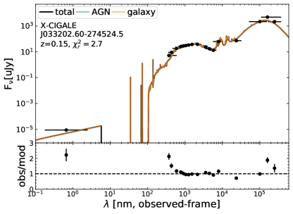
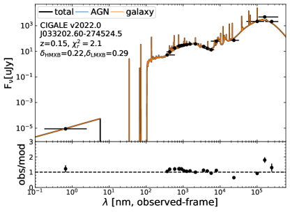
Figure 6: Example SED fits for a CDF-S normal galaxy from x-cigale (left) and cigale v2022.0 (right). The best-fit ${\rm frac_{AGN}}$ is zero in both fits. The observed 0.5–7 keV X-ray flux is much higher than the model one from the x-cigale, but is similar to the one from cigale v2022.0. Also, we note that cigale v2022.0 also has a better fit to the UV data than x-cigale. This is because x-cigale is forced to use a stellar population model that corresponds to a relatively high X-ray flux, although this model does not well fit the observed UV fluxes.

We test the galaxy X-ray modeling in x-cigale using the 7 Ms CDF-S survey, which is the deepest X-ray survey to date (Luo et al., 2017). We take advantage of this unique dataset to study the X-ray emission from normal galaxies in the distant universe, as galaxies’ X-ray power is typically low ($L_{\rm X}\lesssim 10^{42.5}$ erg s^-1) and beyond the sensitivity of most X-ray surveys.

We first select sources classified as “galaxy” instead of “AGN” or “star” by Luo et al. (2017). The classification is based on X-ray and other multiwavelength data. We then restrict the sample to only sources within the GOODS-S field (Guo et al., 2013), where deep multiwavelength coverage is available from UV to FIR. We compile the UV-to-IRAC4 data from Guo et al. (2013) and Spitzer/Herschel mid-to-far IR data from the ASTRODEEP team (Tao Wang 2020, private communication, GOODS-S Herschel catalog). We discard sources with MIPS 24 $\mu$m S/N $<3$, as reliable IR data are essential in constraining SFR (which scales with $L^{\rm HMXB}_{\rm X}$) and possible low-level AGN activity. There are a total of 39 X-ray detected galaxies in our sample. We adopt the redshift measurements compiled by Luo et al. (2017), which are secure spectroscopic redshifts or high-quality photometric redshifts. The redshifts cover a range of $z=0.10$–1.06 (10%–90% percentile), with a median of $z=0.44$.

We first perform SED modeling of these galaxies using x-cigale. The fitting parameters are summarized in Table 2. The galaxy settings are similar to those in §2, except that we allow two metallicity values of $Z=0.004$ and 0.02, as the $L^{\rm HMXB}_{\rm X}$-SFR scaling relation depends on metallicity (e.g., Fragos et al., 2013a). We still allow a moderate AGN component in the fitting (${\rm frac_{AGN}}\leq 0.2$). Although the sources are classified as galaxies by Luo et al. (2017), some could possibly be low-luminosity AGNs (e.g., Young et al., 2012; Ding et al., 2018).

We compare the model versus observed X-ray fluxes in Fig. 5 for x-cigale (left panel). For many (21%) of our sources, the offsets between the model and observed fluxes are more than 0.5 dex. We show an example SED fit with such an issue in Fig. 6 (left). Therefore, x-cigale is not able to model well all of the observed X-ray fluxes.

3.3 Code Improvement

x-cigale assumes that galaxy X-ray emission from HMXBs and LMXBs can be calculated from the scaling relations of $L^{\rm HMXB}_{\rm X}$-SFR and $L^{\rm LMXB}_{\rm X}$-$M_{\star}$ (Fragos et al., 2013a). However, this is an oversimplified assumption, because these relations are just an approximation for the overall galaxy population and scatters around them exist. For example, the content of globular clusters at a given $M_{\star}$, which is not modeled in x-cigale, can significantly affect $L^{\rm LMXB}_{\rm X}$ (e.g., Lehmer et al., 2020). Also, since the HMXB and LMXB emissions are from discrete point sources, $L^{\rm HMXB}_{\rm X}$ and $L^{\rm LMXB}_{\rm X}$ inevitably suffer from statistical fluctuations that are especially strong in low-SFR and/or low-$M_{\star}$ galaxies (e.g., Lehmer et al., 2019, 2021).

To model the $L^{\rm HMXB}_{\rm X}$ and $L^{\rm LMXB}_{\rm X}$ dispersions of individual galaxies in better detail, we introduce two new free parameters, $\delta_{\rm HMXB}$ and $\delta_{\rm LMXB}$, to account for the scatters of the $L^{\rm HMXB}_{\rm X}$-SFR and $L^{\rm LMXB}_{\rm X}$-$M_{\star}$ scaling relations, i.e.,

$$\begin{split}\log(\frac{L_{\rm 2-10\ keV}^{\rm HMXB}}{\rm SFR})=40.3-62Z+569Z^{2}-1834Z^{3}\\ +1968Z^{4}+\delta_{\rm HMXB}\\ \log(\frac{L_{\rm 2-10\ keV}^{\rm LMXB}}{M_{\star}})=40.3-1.5\log t-0.42(\log t)^{2}\\ +0.43(\log t)^{3}+0.14(\log t)^{4}+\delta_{\rm LMXB}\\ \end{split}$$ (4)

where $M_{\star}$ and SFR are in solar units; $t$ denotes stellar age in units of Gyr; $Z$ denotes metallicity (mass fraction). The parameters of $\delta_{\rm HMXB}$ and $\delta_{\rm LMXB}$ are logarithmic deviations from the scaling relations, with positive/negative values meaning higher/lower HMXB and LMXB luminosities, respectively. The user can set multiple values for each parameter to enable a more flexible XRB prescription.

Besides introducing $\delta_{\rm HMXB}$ and $\delta_{\rm LMXB}$, we also implement another update of the code. The code provides three SFR parameters: the instantaneous SFR, the average SFR over 10 Myr, and the average SFR over 100 Myr. While x-cigale adopted the instantaneous SFR when calculating $L^{\rm HMXB}_{\rm X}$, we adopt the average SFR over 100 Myr in cigale v2022.0. This change is because the HMXB emission has strong variability on $\sim 10$ Myr timescales (e.g., Linden et al., 2010; Garofali et al., 2018; Antoniou et al., 2019), but we do not have well-informed calibrations for how the $L^{\rm HMXB}_{\rm X}$ varies on such short timescales. On the other hand, the $L^{\rm HMXB}_{\rm X}$ dependence on longer timescales of $\sim 100$ Myr has been carefully characterized (e.g., Lehmer et al., 2019, 2021). Although the instantaneous SFR and the 100-Myr averaged SFR are similar for a smooth star-formation history (SFH), they can differ significantly if a recent burst/quenching is present in the SFH.

3.4 Results and interpretation

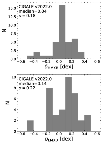
Figure 7: The distributions of $\delta_{\rm HMXB}$ (top) and $\delta_{\rm LMXB}$ (bottom) for CDF-S normal galaxies from the fits of cigale v2022.0. The median and standard deviation are labeled on each panel. The medians are close to zero, indicating that the $L^{\rm HMXB}_{\rm X}$ and $L^{\rm LMXB}_{\rm X}$ scaling relations (Fragos et al., 2013a) are good approximations for the overall galaxy population detected in deep X-ray surveys at $z\lesssim 1$.

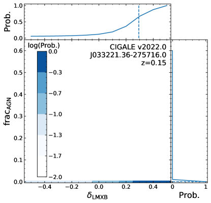
Figure 8: 2D and 1D probability distributions of ${\rm frac_{AGN}}$ and $\delta_{\rm LMXB}$ for the CDF-S normal galaxy in Fig. 6. The plot is generated from the cigale v2022.0 run with ${\rm frac_{AGN}}=0$–0.6. The dashed line indicates the Bayesian (probability-weighted average) values of the two parameters. The ${\rm frac_{AGN}}$ is tightly constrained at a low level ($\lesssim 0.01$) despite the wide allowed ${\rm frac_{AGN}}$ range in the fit. The situations are similar for other sources.

With cigale v2022.0, we re-fit our sample of CDF-S normal galaxies. We set $\delta_{\rm HMXB}$ from $-0.5$ to 0.5 dex with a step of 0.1 dex, while keeping the other parameters unchanged (Table 2). This parameter range is chosen because Lehmer et al. (2021) found the 2$\sigma$ scatter of $L^{\rm HMXB}_{\rm X}/$SFR is $\approx 0.5$ dex at SFR $\approx 4M_{\odot}$ yr^-1, which is the median SFR of our sample. We also set $\delta_{\rm LMXB}$ to the same values as $\delta_{\rm HMXB}$.

Fig. 5 (right) compares the cigale v2022.0 resulting model versus observed X-ray fluxes. The model fluxes agree much better with the observed fluxes compared to those fitted by x-cigale (Fig. 5 left). The offsets between the model and observed are all within 0.5 dex. Fig. 6 (right) shows an example SED fit with cigale v2022.0. For this example, compared to x-cigale, cigale v2022.0 has a better fit not only to the X-ray data but also to the UV data. This is because x-cigale is forced to use a stellar population model that corresponds to a relatively high X-ray emission, although this model does not well fit the observed UV fluxes. This example highlights the importance of introducing $\delta_{\rm HMXB}$ and $\delta_{\rm LMXB}$, without which inappropriate stellar models might be selected.

Fig. 7 displays the distributions of the fitted $\delta_{\rm HMXB}$ and $\delta_{\rm LMXB}$, respectively. Both distributions have slightly positive median values, i.e., 0.04 dex (HMXB) and 0.12 dex (LMXB). These near-zero medians indicate that the $L^{\rm HMXB}_{\rm X}$ and $L^{\rm LMXB}_{\rm X}$ scaling relations (Fragos et al., 2013a) are good approximations for the overall galaxy population detected in deep X-ray surveys at $z\lesssim 1$. The slightly positive trend of the distributions suggest that the scaling relations might have systematic offsets. But the positive trend is expected due to a selection effect, because our X-ray data are flux-limited and thus tend to select higher $L^{\rm HMXB}_{\rm X}$ and $L^{\rm LMXB}_{\rm X}$ sources. A larger normal-galaxy X-ray sample, from, e.g., eROSITA (e.g., Vulic et al., 2021), is needed to investigate the nature the positive trend of $\delta_{\rm HMXB}$ and $\delta_{\rm LMXB}$. Both of the $\delta_{\rm HMXB}$ and $\delta_{\rm LMXB}$ distributions have substantial scatters (standard deviations $\approx 0.2$ dex; Fig. 7). These scatters are likely caused by, e.g., globular-cluster contents and statistical fluctuations (see 3.3).

We set ${\rm frac_{AGN}}\leq 0.2$ in our runs (Table 2) since the sources were classified as normal galaxies by Luo et al. (2017), but this quantitative choice is rather arbitrary. One might worry that our fitting results could heavily depend on the assumption of ${\rm frac_{AGN}}\leq 0.2$, as AGNs can also contribute to the observed X-ray fluxes. To assess the effects of this assumption, we perform a new run including higher ${\rm frac_{AGN}}$ values, i.e., ${\rm frac_{AGN}}=0,0.01,0.03,0.1,0.2,0.3,0.4,0.5,0.6$, while keeping other parameters the same. The resulting $\delta_{\rm HMXB}$ and $\delta_{\rm LMXB}$ distributions are identical to those in Fig. 7, indicating that these two parameters are not strongly degenerate with ${\rm frac_{AGN}}$. Fig. 8 displays example 2D and 1D probability distributions of ${\rm frac_{AGN}}$ and $\delta_{\rm LMXB}$ from the new fit with ${\rm frac_{AGN}}=$0–0.6. The ${\rm frac_{AGN}}$ is tightly constrained at a low level ($\lesssim 0.01$), and the situations are similar for all of our sources. The tight AGN constraints are understandable as the AGN emission is constrained not only by the X-ray data but also by the UV-to-IR data. In summary, we conclude that our fitting results based on the parameters in Table 2 do not depend on the assumption of ${\rm frac_{AGN}}\leq 0.2$.

We set the default values of $\delta_{\rm HMXB}$ and $\delta_{\rm LMXB}$ both to 0, corresponding to the standard Fragos et al. (2013b) scaling relations. For luminous X-ray sources (e.g., $L_{\rm X}\gtrsim 10^{42.5}$ erg s^-1), the observed X-ray fluxes are likely dominated by AGNs, and thus the user can just keep the default values of $\delta_{\rm HMXB}=\delta_{\rm LMXB}=0$. For less luminous sources, galaxy X-ray emission could dominate the observed fluxes, and the user can adopt different values of $\delta_{\rm HMXB}$ and $\delta_{\rm LMXB}$ (e.g., Table 2) to allow more flexible XRB modeling. For specific galaxy populations, the user could allow multiple values for only one of $\delta_{\rm HMXB}$ and $\delta_{\rm LMXB}$ to save memory and reduce computation time. For example, for quiescent galaxies, $L^{\rm HMXB}_{\rm X}$ should be negligible compared to $L^{\rm LMXB}_{\rm X}$. In this case, the user can adopt multiple values for $\delta_{\rm LMXB}$ while keeping $\delta_{\rm HMXB}=0$.

4 Flexible UV/optical SED shape of AGN accretion disk

4.1 Motivation

x-cigale adopts a single fixed SED shape of an AGN accretion disk from Schartmann et al. (2005), which is a broken power-law. Although the Schartmann et al. (2005) recipe is a good approximation for the overall disk SED shape, it might not be sufficiently accurate for individual sources. This is because the observed UV/optical slopes of type 1 quasars have non-negligible intrinsic dispersions (e.g., Elvis et al., 1994), possibly due to different black-hole masses, accretion rates, and spins (e.g., Koratkar & Blaes, 1999).

4.2 Sample and preliminary fitting

Table 3: Model parameters for the SDSS quasars

Module	Parameter	Symbol	Values
AGN (UV-to-IR) SKIRTOR	AGN contribution to IR luminosity	${\rm frac_{AGN}}$	0.9999
	Viewing angle	$\theta$	30∘
	Polar-dust color excess	$E(B-V)_{\rm PD}$	0., 0.01, 0.02, 0.05, 0.1, 0.15, 0.2, 0.3, 0.4, 0.5, 0.6 mag
	Intrinsic disk type	–	Schartmann et al. (2005)
	Deviation from the default UV/optical slope	$\boldsymbol{\delta_{\rm AGN}}$	$\boldsymbol{-1}$ to 1 (step 0.1)
X-ray	AGN photon index	$\Gamma$	1.8
	Maximum deviation from the $\alpha_{\rm ox}$-$L_{\nu,2500\textup{\AA}}$ relation	$|\Delta\alpha_{\rm ox}|_{\rm max}$	0.2

Note. — For parameters not listed here, we use the default values. Bold font indicates new parameters in cigale v2022.0 introduced in this work.

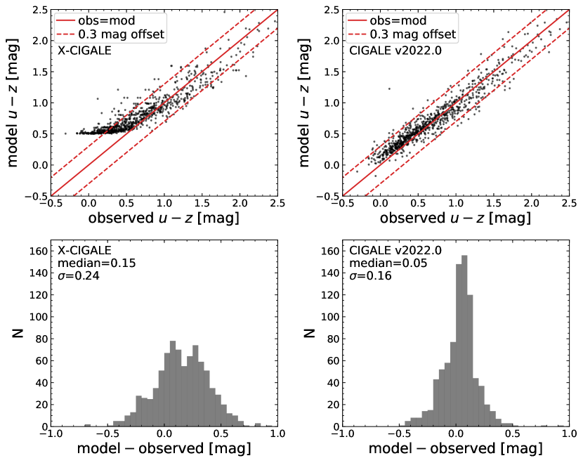
Figure 9: Top: Model versus observed $u-z$ color of our SDSS quasars from x-cigale (left) and cigale v2022.0 (right). The red solid line indicates a model$=$observed relation; the red dashed lines indicate 0.3 mag offsets from this relation. We only plot points for sources having both $u$ and $z$ S/N$>5$. Bottom: The distributions of model$-$observed $u-z$ color from x-cigale (left) and cigale v2022.0 (right). The median and standard-deviation values are labeled on each panel. The observed $u-z$ color can be bluer than $0.5$ mag. This cannot be re-produced with x-cigale, where the AGN disk SED shape is fixed. But cigale v2022.0 can account for these blue SEDs with $u-z<0.5$ mag.

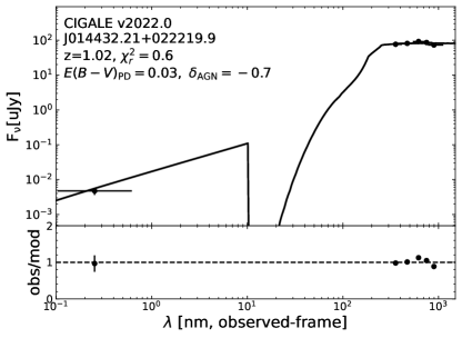
Figure 10: Example SED fits for an SDSS quasar from x-cigale (left) and cigale v2022.0 (right). This source has observed UV/optical SED bluer than the model SED of Schartmann et al. (2005), and thus it cannot be fitted well with x-cigale. cigale v2022.0 allows a flexible model that can account for the blue SED shape.

To test whether this single spectral shape is sufficient to account for the observed SEDs, we use the SDSS DR14 type 1 quasar sample (Pâris et al., 2018) that has XMM-Newton X-ray detections (see §3.1.1 of Yang et al. 2020 for the details). We further apply a magnitude cut ($r_{\rm AB}<21.8$ mag) and a redshift cut ($z>1$) to ensure that the observed SEDs are dominated by AGNs, as SDSS normal galaxies with $r_{\rm AB}<21.8$ mag are always below $z=1$ (e.g., Sheldon et al., 2012). Therefore, these cuts allow us to model SEDs with pure AGN templates as below, avoiding potential degeneracy issues (see §4.4).

The final sample has 1080 sources. We run x-cigale on the SDSS $ugriz$ and the 2–10 keV fluxes. The inclusion of X-ray photometry is to better constrain the AGN intrinsic emission. The fitting parameters are listed in Table 3. We set ${\rm frac_{AGN}}$ (fractional AGN IR luminosity) to a value close to unity (0.9999), so that the observed UV/optical SED is totally AGN dominated, which is the case for the SDSS quasars after our magnitude and redshift cuts. We also allow different levels of polar-dust extinction.

We compare the resulting x-cigale model versus observed $u-z$ colors in Fig. 9 (left). In this figure, we only consider sources having both $u$ and $z$ signal-to-noise ratios (S/N) above 5. One notable issue is that a “plateau” exists at model $u-z\approx 0.5$. This is because the model $u-z$ cannot be bluer than the intrinsic disk color ($u-z=0.5$) but a significant fraction (32%) of sources have observed $u-z<0.5$. Due to this issue, the offsets between the model and observed $u-z$ have a positive median value of 0.15. Fig. 10 (left) shows an example SED. The observed SED is even bluer than the zero-extinction model SED. To address this issue, it is necessary to allow a flexible SED shape for AGN intrinsic-disk emission.

4.3 Code improvement

To allow for deviations from the default Schartmann et al. (2005) optical spectral slope as suggested by the observed quasars (§4.2), we introduce a free parameter, $\delta_{\rm AGN}$, i.e.,

$$\lambda L_{\lambda}\propto\left\{\begin{array}[]{lr}\lambda^{2}&0.008\leq\lambda\leq 0.05\ [\mu\mathrm{m}]\\ \lambda^{0.8}&0.05<\lambda\leq 0.125\ [\mu\mathrm{m}]\\ \lambda^{-0.5+\delta_{\rm AGN}}&0.125<\lambda\leq 10\ [\mu\mathrm{m}]\\ \lambda^{-3}&10<\lambda\leq 1000\ [\mu\mathrm{m}]\end{array}\right.$$ (5)

In cigale v2022.0, we also allow the user to choose the disk continuum from the SKIRTOR model (Stalevski et al., 2012, 2016), i.e.,

$$\lambda L_{\lambda}\propto\left\{\begin{array}[]{lr}\lambda^{1.2}&0.008\leq\lambda\leq 0.01\ [\mu\mathrm{m}]\\ \lambda^{0}&0.01<\lambda\leq 0.1\ [\mu\mathrm{m}]\\ \lambda^{-0.5+\delta_{\rm AGN}}&0.1<\lambda\leq 5\ [\mu\mathrm{m}]\\ \lambda^{-3}&5<\lambda\leq 1000\ [\mu\mathrm{m}]\end{array}\right.$$ (6)

From Eqs. 5 and 6 the major differences between the Schartmann et al. (2005) and SKIRTOR disk continuum are the wavelength boundaries and power-law indices at far-UV ($\lambda<125$ nm), where observational constraints are weaker compared to those at longer wavelengths (e.g., Stevans et al., 2014; Lusso et al., 2015).

4.4 Results and interpretation

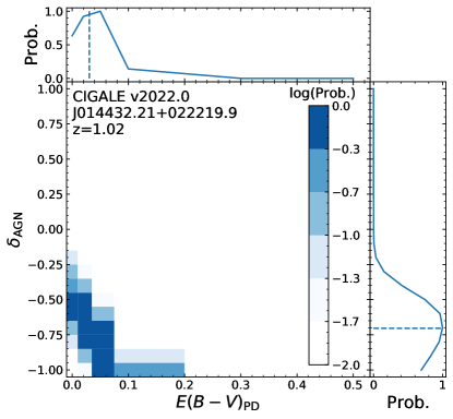
Figure 11: 2D and 1D probability distributions of $\delta_{\rm AGN}$ and $E(B-V)_{\rm PD}$ for the SDSS quasar in Fig. 10, generated from the cigale v2022.0 run. The dashed line indicates the Bayesian (probability-weighted average) values of the two parameters. From the color-coded 2D probability distribution, the $\delta_{\rm AGN}$ and $E(B-V)_{\rm PD}$ are anti-correlated, indicating a degeneracy between these two parameters.

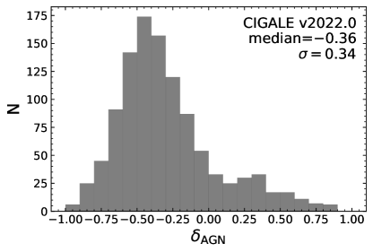
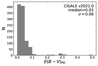
Figure 12: Distribution of the $\delta_{\rm AGN}$ and $E(B-V)_{\rm PD}$ for the SDSS quasar sample from the fits with cigale v2022.0. The median and standard deviation values for the distributions are labeled on corresponding panels. The $\delta_{\rm AGN}$ values tend to be negative (i.e., bluer than the default Schartmann et al. 2005 SED model).

We re-fit the SDSS quasar SEDs using cigale v2022.0. We still adopt the Schartmann et al. (2005) disk SED shape (Eq. 5), since it agrees better with observations than the SKIRTOR disk model (Eq. 6; e.g., Duras et al., 2017). We allow $\delta_{\rm AGN}$ to vary from $-1$ to 1 with a step of 0.1 (see Table 3). This $\delta_{\rm AGN}$ range covers nearly all of the observed SED slope variations in the SDSS quasar sample of Davis et al. (2007, see their Fig. 2).

We compare the model versus observed $u-z$ colors in Fig. 9 (right). The model colors agree better with the observed colors than those from the x-cigale fits. The median offset of the model and observed $u-z$ is close to zero (0.05), while the x-cigale fits have a median of 0.15. Also, the scatter has been reduced from 0.24 (x-cigale fits) to 0.16 (cigale v2022.0 fits). Fig. 10 (right) shows an example SED fit. The observed SED can be well fitted with a reduced $\chi_{r}^{2}=0.6$ (the value is 3.4 for the x-cigale fit). Fig. 11 displays the 2D and 1D probability distributions of $\delta_{\rm AGN}$ and $E(B-V)_{\rm PD}$ of this example fit. There is an anti-correlation between $\delta_{\rm AGN}$ and $E(B-V)_{\rm PD}$ in the 2D probability distribution. This anti-correlation is expected, because, e.g., a higher $\delta_{\rm AGN}$ (redder intrinsic slope) and a lower $E(B-V)_{\rm PD}$ (weaker polar-dust extinction) can roughly cancel out the effect of each other. Therefore, there is a natural degeneracy between these two parameters.

Fig. 12 displays the distribution of the fitted $\delta_{\rm AGN}$ and $E(B-V)_{\rm PD}$. The median of the $\delta_{\rm AGN}$ distribution is $-0.36$ with a significant scatter of 0.34. This negative median value could be intrinsic, as the default Schartmann et al. (2005) spectral shape is based on the observed quasar SEDs, without considering polar-dust extinction. Indeed, the polar-dust extinctions are non-negligible [median $E(B-V)_{\rm PD}=0.03$], although heavy extinctions of $E(B-V)_{\rm PD}>0.1$ are rare (6%). However, we note that the degeneracy between $\delta_{\rm AGN}$ and $E(B-V)_{\rm PD}$ (e.g., Fig. 11) might also contribute to the negative trend of $\delta_{\rm AGN}$. We caution that both of the $\delta_{\rm AGN}$ and $E(B-V)_{\rm PD}$ distributions quantitatively depend on the adopted specific extinction law. We adopt the default SMC law here, and refer to Buat et al. (2021) for a detailed discussion of the effects of different laws.

Given the degeneracy between $\delta_{\rm AGN}$ and $E(B-V)_{\rm PD}$, one might think of adapting the original disk SED shapes (Schartmann and SKIRTOR; §4.3) to the bluest variation in our sample and attributing all observed SED variations to $E(B-V)_{\rm PD}$. This idea has the benefit of simplicity, but we do not adopt it for three reasons. First, it is unlikely that all AGNs share the same intrinsic SED shape over wide ranges of BH masses and accretion rates (e.g., Whiting et al., 2001; Richards et al., 2003). Second, the current approach is more flexible than adapting the template, and the philosophy of cigale highlights flexibility rather than simplicity. Third, although $E(B-V)_{\rm PD}$ and $\delta_{\rm AGN}$ are degenerate over UV/optical wavelengths, they can be better differentiated given excellent IR coverage, because dust-reddened AGNs have polar-dust IR re-emission (included in cigale) but intrinsically red AGNs do not. In cigale, polar dust is an obscuration structure with optical depth much smaller than the torus (see §2.4 of Yang et al. 2020 for details). cigale assumes that the polar-dust IR emission follows a “grey body” model (e.g., Casey, 2012) with temperature and emissivity as free parameters. Future IR missions, e.g., JWST and Origins, will be able to detect (tightly constrain) the polar-dust IR re-emission and thereby differentiate the two cases of dust-reddened vs. intrinsically red SEDs.

We set the default $\delta_{\rm AGN}$ and $E(B-V)_{\rm PD}$ to the median values of our fits, i.e., $\delta_{\rm AGN}=-0.36$ and $E(B-V)_{\rm PD}=0.03$. When fitting type 1 AGNs, the user is recommended to adopt multiple values of these two parameters (such as those in Table 3), because both parameters have significant scatters based on our fits (see Fig. 12). When fitting type 2 AGNs, for which the AGN disk emission is almost entirely obscured by the dusty torus, the user can keep the default $\delta_{\rm AGN}$ to save memory and reduce computational time. However, it is still recommended to adopt multiple values of $E(B-V)_{\rm PD}$ when mid-to-far IR coverage is available for the type 2 sources, because $E(B-V)_{\rm PD}$ sets the strength of polar-dust re-emission that could contribute significantly at IR wavelengths.

Finally, we stress the importance of our redshift and magnitude cuts (§4.2). These cuts guarantee the observed SEDs are dominated by AGNs, allowing us to model the data with pure AGN templates. Actually, we have tested fits with AGN$+$galaxy mixed templates by freeing ${\rm frac_{AGN}}$, and found our parameters of interest ($\delta_{\rm AGN}$ and $E(B-V)_{\rm PD}$) could be significantly affected. This is because a blue observed SED can be either explained by a low-dust star-forming galaxy component or an AGN component. Fig. 13 displays such an AGN-galaxy degeneracy for an SDSS quasar, for which $\delta_{\rm AGN}$ and $E(B-V)_{\rm PD}$ are strongly affected when a galaxy component is allowed. Therefore, our redshift/magnitude cuts and pure-AGN approach are crucial for our investigation of $\delta_{\rm AGN}$ and $E(B-V)_{\rm PD}$. The user who is interested in these parameters should be cautious of the degeneracy effects, when modeling SEDs that have non-negligible galaxy components. On the other hand, some studies indicate that some other source properties such as ${\rm frac_{AGN}}$, AGN bolometric luminosity ($L_{\rm AGN}$), and SFR are not strongly affected by the degeneracy issue, especially when good multiwavelength coverage is available (e.g., Mountrichas et al., 2021c; Yang et al., 2021; Thorne et al., 2022). This is understandable, considering that those properties can be constrained by multiwavelength data simultaneously, e.g., $L_{\rm AGN}$ is related to X-ray, UV/optical, and IR wavelengths. However, in contrast, $\delta_{\rm AGN}$ and $E(B-V)_{\rm PD}$ are very sensitive to the detailed SED-shape modeling at UV/optical wavelengths, and thus they are more strongly affected by the AGN-galaxy degeneracy than properties like $L_{\rm AGN}$.

Figure 13: Example SED fits for an SDSS quasar using AGN$+$galaxy mixed models (left) and pure AGN models (right; the approach in our analysis). Both fits can explain the observed SED data, indicating that quasar and blue star-forming templates are degenerate. The resulting $E(B-V)_{\rm PD}$ and $\delta_{\rm AGN}$ (as labeled) are quite different for the two fits, indicating the degeneracy can significantly affect these parameters. Since the galaxy component on the left panel is unrealistic (see §4.2), we adopt pure AGN models in our analysis to avoid the degeneracy issue.

5 AGN radio emission

5.1 Motivation

x-cigale can only account for radio emission from star formation (SF; Boquien et al., 2019). This SF radio emission has two components: one is a thermal component contributed by the “nebular” module; the other is a synchrotron component contributed by the “radio” module. The latter is often dominant, and is calculated in x-cigale using the radio-IR correlation parameter $q_{\rm IR}$ (e.g., Helou et al., 1985), i.e.,

$$q_{\rm IR}=\log\left(\frac{L_{\rm SF,IR}}{L_{\nu,21\rm cm}\times 3.75\times 10^{12}\rm\ Hz}\right)$$ (7)

where $L_{\rm SF,IR}$ is the total star-forming IR luminosity (mostly in FIR) and $L_{\nu,21\rm cm}$ is the corresponding radio synchrotron luminosity at 21 cm (1.4 GHz). The default value of $q_{\rm IR}$ is 2.58 in x-cigale. Besides $q_{\rm IR}$, which sets the normalization at 21 cm, there is another free parameter ($\alpha_{\rm SF}$) that controls the power-law slope of the SF synchrotron emission, i.e.,

$$L_{\nu,\rm SF}\propto\nu^{-\alpha_{\rm SF}}.$$ (8)

The default value of $\alpha_{\rm SF}$ is 0.8 in both x-cigale and cigale v2022.0.

x-cigale does not have AGN emission at radio wavelengths. However, AGNs may have powerful jets that emit strong radio radiation (i.e., radio-loud AGNs), and the jets can play an important role in AGN-galaxy coevolution (e.g., Fabian, 2012). The physical origin of AGN radio jets is still controversial. One popular theory is the BZ (Blandford-Znajek) process (e.g., Blandford & Znajek, 1977; Blandford et al., 2019). The BZ mechanism considers that the jet is powered by the rotational energy of the black hole (BH) through the magnetic field threading the horizon (e.g., Davis & Tchekhovskoy, 2020). Recent observations suggest that the magnetic flux/topology close to the BH instead of the BH spin could be the determining factor of the jet-launching process (e.g., Zhu et al., 2020). Besides the jets, other processes such as AGN winds, coronae, and shocks can also emit at radio wavelengths (e.g., Panessa et al., 2019).

5.2 Sample and preliminary fitting

Table 4: Model parameters for the COSMOS radio sources

Module	Parameter	Symbol	Values
Star formation history $\mathrm{SFR}\propto t\exp(-t/\tau)$	Stellar e-folding time	$\tau_{\rm star}$	0.1, 0.5, 1, 5 Gyr
	Stellar age	$t_{\rm star}$	0.5, 1, 3, 5, 7 Gyr
Simple stellar population Bruzual & Charlot (2003)	Initial mass function	$-$	Chabrier (2003)
	Metallicity	$Z$	0.02
Dust attenuation Calzetti et al. (2000)	Color excess of the nebular lines	$E(B-V)$	0.05, 0.1, 0.2, 0.3, 0.4, 0.5, 0.6 mag
Galactic dust emission: Dale et al. (2014)	Slope in $dM_{\rm dust}\propto U^{-\alpha}dU$	$\alpha$	2
AGN (UV-to-IR) SKIRTOR	AGN contribution to IR luminosity	${\rm frac_{AGN}}$	0–0.99 (step 0.1)
	Viewing angle	$\theta$	30∘, 70∘
	Polar-dust color excess	$E(B-V)_{\rm PD}$	0, 0.2, 0.4 mag
Radio	SF radio-IR correlation parameter	$q_{\rm IR}$	2.4, 2.5, 2.6, 2.7
	SF power-law slope	$\alpha_{\rm SF}$	0.8
	Radio-loudness parameter	$\boldsymbol{R_{\rm AGN}}$	0.01, 0.02, 0.05, 0.1, 0.2, 0.5, …, 1000, 2000, 5000, 10000
	AGN power-law slope	$\boldsymbol{\alpha_{\rm AGN}}$	0.7

Note. — For parameters not listed here, we use the default values. Bold font indicates new parameters in cigale v2022.0 introduced in this work.

Figure 14: Top: Model versus observed 3 GHz flux density of our COSMOS radio sources from x-cigale (left) and cigale v2022.0 (right). The red solid line indicates a model$=$observed relation; the red dashed lines indicate 0.3 dex offsets from this relation. Bottom: The distributions of logarithmic model/observed $f_{\nu,\rm 3GHz}$ from the x-cigale (left) and cigale v2022.0 (right). x-cigale systematically underestimates $f_{\nu,\rm 3GHz}$, indicating the presence of radio AGN emission. This underestimation does not exist for the fits of cigale v2022.0, which has an AGN radio component.

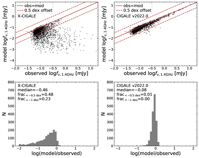
Figure 15: Same format as Fig. 14 but for the 1.4 GHz band.

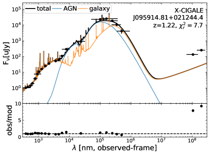
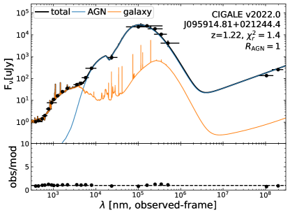
Figure 16: Example SED fits for a COSMOS radio source from x-cigale (left) and cigale v2022.0 (right). The observed radio fluxes are much higher than the model ones from x-cigale. cigale v2022.0 accounts for this radio excess with an AGN radio component. Also, compared to the cigale v2022.0 fit, the x-cigale fit has much stronger galaxy IR component, because the high observed radio fluxes force an elevated galaxy IR emission via $q_{\rm IR}$ (Eq. 7).

Similar to the procedures of the previous sections (§2, §3, and §4), we first compile a proper radio-selected sample and then perform SED modeling with x-cigale in this section. We adopt all of the $>5\sigma$ radio detections in the VLA-COSMOS 3 GHz Large Project (Smolčić et al., 2017a, b). We also collect the VLA 1.4 GHz fluxes when available from Schinnerer et al. (2010). Delvecchio et al. (2017) matched the radio sources to the COSMOS2015 catalog (Laigle et al., 2016). We adopt these matching results and obtain the UV-to-IRAC4 broad-band photometry (14 bands) from COSMOS2015. We discard the radio sources without COSMOS2015 counterparts, as the UV-to-IRAC4 data are necessary to model the stellar population. The sample contains 6497 sources in total. We also include Spitzer/MIPS (24 $\mu$m), Herschel/PACS (100 $\mu$m and 160 $\mu$m), and Herschel/SPIRE (250 $\mu$m, 350 $\mu$m, and 500 $\mu$m) photometry from the “super-deblended” catalog of Jin et al. (2018). We do not include X-ray fluxes here due to the reason presented in §5.4, i.e., we want to keep our SED fits and subsequent source classifications independent from the X-ray information. We adopt the redshift measurements from Delvecchio et al. (2017), which are spec-$z$ (if available) or photo-$z$. The median redshift is 1.18 and the 10%–90% percentile range is $z=0.42$–2.56.

We first fit the photometric data above with x-cigale. The model parameters are listed in Table 4. We set $q_{\rm IR}$ to a range of 2.4–2.7 (step 0.1), based on the observations of Delvecchio et al. (2021). Fig. 14 (left) and Fig. 15 (left) display the resulting model fluxes versus the observed values for 3 GHz and 1.4 GHz, respectively. The model fluxes are systematically lower than the observed ones, e.g., 28% (11%) of sources have observed 3 GHz fluxes more than 3 (10) times higher than the model fluxes. In contrast, no sources have model fluxes $>3$ times higher than the observed values. This result of “radio excess” strongly indicates that an AGN radio component is needed to explain the observed radio fluxes for many sources. Fig. 16 (left) shows an example SED fit with significant radio excess.

5.3 Code improvement

We add a new AGN component to the radio module of x-cigale. To quantitatively model AGN radio emission, we employ the radio-loudness parameter, $R$, defined as (e.g., Ballo et al., 2012),

$$R_{\rm AGN}=\frac{L_{\rm\nu,5GHz}}{L_{\nu,2500\textup{\AA}}},$$ (9)

where $L_{\rm\nu,5GHz}$ and $L_{\nu,2500\textup{\AA}}$ are the monochromatic AGN luminosities per frequency at rest-frame 5 GHz and 2500 $\rm\AA$, respectively. $R_{\rm AGN}$ is a free parameter that allows any values $\geq 0$ ($R_{\rm AGN}=0$ means no AGN radio emission).

Here, we adopt $L_{\nu,2500\textup{\AA}}$ as the intrinsic (polar-dust absorption corrected) luminosity observed at a viewing angle of $30^{\circ}$, and this quantity is available for x-cigale models (see §2). This definition ensures that $R$ is a physical quantity inherent to the AGN itself and does not depend on the viewing angle (e.g., Padovani, 2016; Padovani et al., 2017). Therefore, $R$ works consistently for both type 1 and type 2 AGNs. Currently, we assume $L_{\rm\nu,5GHz}$ is isotropic in x-cigale. In the future, we will model the radio anisotropy, which can be important for, e.g., blazars and BL Lac objects.

We assume a power-law AGN SED over the wavelength range of 0.1–1000 mm, i.e.,

$$L_{\nu,\rm AGN}\propto\nu^{-\alpha_{\rm AGN}},$$ (10)

where we allow the user to freely set the $\alpha_{\rm AGN}$ slope. We set the default value as $\alpha_{\rm AGN}=0.7$ (e.g., Randall et al., 2012; Tiwari, 2019). We caution that the power-law shape is an overall simplistic assumption, as the real AGN radio SEDs might be more complicated. The formula in Eq. 10 mainly serves as a correction for the AGN contribution to radio fluxes, especially for the cases where only one or two radio bands are available like our COSMOS radio sample. In the future, we will explore more realistic and complicated radio models based on multi-band radio data.

5.4 Results and interpretation

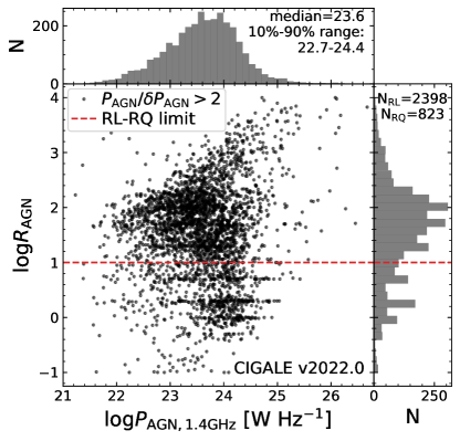
Figure 17: $R_{\rm AGN}$ versus AGN 1.4 GHz power and their distributions. Only the sources with a significant AGN component ($P_{\rm AGN,1.4GHz}/\delta P_{\rm AGN,1.4GHz}>2$) are displayed. The red dashed horizontal line indicates the threshold for our radio-loud versus radio-quiet classification.

Figure 18: X-ray detection fraction for different radio source types (as labeled). The red data point represents the radio AGN sample ($P_{\rm AGN,1.4GHz}/\delta P_{\rm AGN,1.4GHz}>2$), including both RL and RQ AGNs. The error bars represent binomial uncertainties. The radio AGNs have a higher X-ray detection fraction than the SF galaxies, suggesting a link between AGN radio and X-ray emission.

Using cigale v2022.0, we re-fit the photometric data of the COSMOS radio sources (§5.1). We set $R_{\rm AGN}$ to a wide logarithmic-spaced grid from 0.01 to 10000 (see Table 4) based on the observations of quasars (e.g., Zhu et al., 2020). We fix the radio slope in Eq. 10 at the default value of $\alpha_{\rm AGN}=0.7$, as most (73%) of our sources only have one radio band (3 GHz) available.

Unlike the results from x-cigale, the model radio fluxes agree well with the observed fluxes (see Figs. 14 & 15). The offsets between model and observed radio fluxes are mostly (99.91% for 3 GHz and 98.6% for 1.4 GHz) within 0.5 dex. Therefore, we conclude that our implementation of the AGN radio component is indeed useful in explaining the observed radio flux, although the good fit of radio data is not surprising given only one (or two) radio band(s) is available for each source in our sample. Interestingly, the model 1.4 GHz fluxes tend to be slightly lower than the observed ones (median offset $=0.08$ dex), suggesting that the typical AGN radio SED in the COSMOS sample is steeper than our assumed $\alpha_{\rm AGN}=0.7$ (Table 4). However, this systematic offset might also be a selection effect, as the relatively shallow 1.4 GHz data may miss AGNs with flatter radio SEDs and thereby lower 1.4 GHz fluxes.

Fig. 16 compares example SED fits from x-cigale and cigale v2022.0. The observed radio fluxes are dominated by the AGN component from the cigale v2022.0 fit. The x-cigale fit is not able to explain the radio fluxes due to the lack of AGN radio emission. Compared to the cigale v2022.0 fit, the x-cigale fit has a stronger galaxy IR component. This is because x-cigale only has galaxy radio emission which is related to galaxy IR emission through the radio-IR correlation (§5.1). The high observed radio flux forcibly elevates not only galaxy radio emission but also its IR emission as a consequence. In the cigale v2022.0 fit, the radio flux is mostly explained by the AGN component, and thus the strong requirement of a galaxy component is relaxed.

cigale v2022.0 can calculate AGN rest-frame 1.4 GHz luminosity ($P_{\rm AGN,1.4GHz}$; e.g., Padovani 2016) as a measure of AGN radio strength. In this work, we consider the sources with $P_{\rm AGN,1.4GHz}/\delta P_{\rm AGN,1.4GHz}>2$ (where $\delta P_{\rm AGN,1.4GHz}$ is the $P_{\rm AGN,1.4GHz}$ uncertainty from cigale v2022.0) as radio AGNs and the rest as radio SF galaxies. This definition guarantees that the AGN radio component is statistically significant ($>2\sigma$) for the classified radio AGNs. We note that our definition of AGN/SF is based on the radio-band decomposition, because our focus here is radio emission. For example, if a source has AGN features at other wavelengths (e.g., X-ray; see below) but its AGN radio emission is insignificant, it will be classified as a radio SF galaxy here. There are a total of 3221 radio AGNs, 50% of the sample. This high fraction indicates that radio AGNs are common among the sources selected by deep radio surveys. The radio-AGN fraction depends on radio fluxes. The fractions are 47% and 85% for sources with 3 GHz fluxes below and above 0.2 mJy, respectively. This significant radio-flux dependence is also found by Smolčić et al. (2017b), who used empirical criteria to classify AGNs and SF galaxies.

Fig. 17 displays $R_{\rm AGN}$ versus $P_{\rm AGN,1.4GHz}$ and their distributions for our radio AGNs ($P_{\rm AGN,1.4GHz}/\delta P_{\rm AGN,1.4GHz}>2$). The red dashed line marks the conventional threshold (i.e., $R_{\rm AGN}=10$; Kellermann et al. 1989) for radio-quiet (RQ) versus radio-loud (RL) AGN classifications. The numbers of RQ and RL AGNs are 823 (26%) and 2398 (74%), respectively. We remind the reader that this RQ/RL classification demonstrates an advantage of cigale v2022.0, which simultaneously models multiwavelength data in a consistent way (§5.3). Such a task is challenging for empirical approaches, because the AGN UV/optical emission is often heavily obscured and not directly observable (e.g., Fig. 16).

X-ray emission is a good tracer of the BH-accretion process (e.g., Brandt & Alexander, 2015; Brandt & Yang, 2021). It is intriguing to investigate the X-ray emission of our classified radio types. We adopt the Chandra COSMOS-Legacy survey (Civano et al., 2016; Marchesi et al., 2016). A total of 801 of the radio-selected sources in our radio sample are detected in X-ray. Fig. 18 displays the fractions of X-ray detected sources among different radio types. The error bars represent binomial uncertainties calculated using astropy.stats.binom_conf_interval. The uncertainties are negligible compared to the differences across different radio types, thanks to our relatively large sample sizes.

The X-ray fraction of the radio AGNs is 1.9 times higher than that of the radio SF. This result indicates that there is a positive link between AGN radio and X-ray emission, broadly consistent with the findings in the literature (e.g., Merloni et al., 2003; Laor & Behar, 2008). Among the radio AGNs, the RQ population has a higher X-ray detected fraction than the RL population (Fig. 18). This is expected, because RQ should have higher $L_{\nu,2500\textup{\AA}}$ than RL at a given $P_{\rm AGN,1.4GHz}$ (see Eq. 9), and $L_{\nu,2500\textup{\AA}}$ is strongly correlated with AGN $L_{\rm X}$ due to the $\alpha_{\rm ox}$-$L_{\nu,2500\textup{\AA}}$ relation (e.g., Steffen et al., 2006; Just et al., 2007). However, the X-ray fraction of the RL AGNs is still significantly higher than that of the radio SF population (13% vs. 9%). Assuming that the radio emission in RL AGNs is mainly from jets (§5), the elevated X-ray fraction of the RL population suggests a connection between jets and X-ray emission. This connection suggests that AGN jets could actively produce X-rays (e.g., Harris & Krawczynski, 2006), or that there is a positive link between jets and the X-ray emitting coronae (e.g., Zhu et al., 2020).

We note that, since we do not include the X-ray data in our x-cigale run (§5.2), the X-ray detection fraction is independent of our SF, RQ, and RL classifications. Therefore, the X-ray fraction dependence on the radio type should be intrinsic, not a bias due to our SED-fitting procedure.

We set the default $\alpha_{\rm AGN}=0.7$ (see §5.3) and $R_{\rm AGN}=10$ (i.e., the boundary between RL and RQ AGNs). For $\alpha_{\rm AGN}$, when there are multi-frequency radio data spanning a large wavelength range, the user can adopt multiple $\alpha_{\rm AGN}$ values to better model the observed radio fluxes. When only one or two radio bands within a narrow wavelength range (like our case) are available, the user can just keep the default $\alpha_{\rm AGN}$ to save memory and reduce computational time. For the parameter of $R_{\rm AGN}$, we recommend the user to adopt multiple values based on our fits (e.g., Fig. 17). The user can narrow the range of $R_{\rm AGN}$ in some cases. For example, if the sources have spatially extended radio structures (strong evidence for radio-loud AGNs), then $R_{\rm AGN}$ can be set to $>10$ values.

6 Miscellaneous Updates

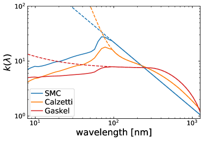
Figure 19: Top: The extinction curves in cigale v2022.0 (solid) and x-cigale (dashed). Different colors indicate different extinction laws as labeled. Below 100 nm the cigale v2022.0 curves have been obtained calculated based on the optical properties of the realistic dust mixtures, while the x-cigale curves are analytical extrapolation. Bottom: The type 1 AGN SED models with different polar-dust $E(B-V)$. The models are normalized at 10 $\mu$m. The solid and dashed curves are based on the cigale v2022.0 and x-cigale SMC extinction curves, respectively. The polar-dust re-emission ($\sim 30\ \mu$m) is lower (bottom panel) when using the cigale v2022.0 extinction, because the cigale v2022.0 extinction is weaker than the x-cigale one at $<10$ nm and both codes follow energy conservation.

Besides the major changes of the code detailed in previous sections, we also implement several minor updates as below.

• In x-cigale, the $\alpha_{\rm ox}$ parameter (X-ray module) is internally set to $-1.9$, $-1.8$, $-1.7$, …, $-1.1$, and the user cannot control it. In cigale v2022.0, we change $\alpha_{\rm ox}$ to an explicit parameter that is set by the user, although the default values are still $-1.9$, $-1.8$, …, $-1.1$.

  This change allows the user to run x-cigale more effectively when using the X-ray module. For example, if the sample consists of luminous quasars which typically have more negative values of $\alpha_{\rm ox}$ (e.g., Just et al., 2007), then the user can set $\alpha_{\rm ox}$ as, e.g., $-1.9$, $-1.8$, $-1.7$, and $-1.6$. This setting will reduce the number of models by a factor of 2.25, significantly boosting the efficiency.

  This update of $\alpha_{\rm ox}$ also allows the investigations of rare AGNs that have extreme $\alpha_{\rm ox}$ values. For example, the class of X-ray weak quasars can have $\alpha_{\rm ox}<-1.9$ (e.g., Pu et al., 2020), beyond the fixed $\alpha_{\rm ox}$ parameter grid in x-cigale. In cigale v2022.0, the user can adopt $\alpha_{\rm ox}$ more negative than $-1.9$ to probe the X-ray weak population.

• In x-cigale, the normalization of the AGN component is controlled by the parameter of AGN fraction, defined as ${\rm frac_{AGN}}=\frac{L_{\rm dust,AGN}}{L_{\rm dust,AGN}+L_{\rm dust,galaxy}}$, where $L_{\rm dust,AGN}$ and $L_{\rm dust,galaxy}$ are AGN and galaxy dust luminosity (integrated over all wavelengths), respectively. In cigale v2022.0, we allow the user to change the definition wavelength (range) of ${\rm frac_{AGN}}$ by another parameter, “lambda_fracAGN”. Setting it to “$\lambda_{\rm min}/\lambda_{\rm max}$” (units: $\mu$m) means that ${\rm frac_{AGN}}$ is defined as $\frac{L_{\rm AGN}}{L_{\rm AGN}+L_{\rm galaxy}}$, where $L_{\rm AGN}$ and $L_{\rm galaxy}$ are AGN and galaxy total luminosity (not only dust) integrated over the wavelength range from $\lambda_{\rm min}$ to $\lambda_{\rm max}$. If $\lambda_{\rm min}=\lambda_{\rm max}$, then the code will use the monochromatic luminosity at this wavelength. If lambda_fracAGN is set to “0/0” (the default values), then the code will still use the definition of ${\rm frac_{AGN}}$ in x-cigale. This change allows the users to model AGN versus galaxy relative strength in their interested wavelengths.

• x-cigale allows three extinction laws for AGN polar dust, i.e., Calzetti et al. (2000, nearby star-forming galaxies), Gaskell et al. (2004, large dust grains), and Prevot et al. (1984, Small Magellanic Cloud, SMC). These extinction laws extend to $\approx 100$ nm, below which x-cigale adopts analytical extrapolations. These extrapolations lead to large, non-physical extinctions below $100$ nm. This has a direct impact in the models, the dust reprocessing too much radiation that is re-emitted in the infrared while dramatically steepening the slope of the accretion-disk emission. In order to address this issue, the extinction curves were recalculated in the entire wavelength range of interest by the module within the skirt radiative-transfer code (Baes et al., 2011; Baes & Camps, 2015; Camps & Baes, 2015) based on the realistic dust mixtures and optical properties taken from the literature. The SMC dust mixture consists of populations of silicate and graphite dust grains. The grain size distribution is taken from Weingartner & Draine (2001): a power-law function with a curvature and an exponential cutoff. Instead of extrapolation, below 100 nm, Calzetti extinction curve was replaced by the one corresponding to the standard Galactic interstellar dust (Mathis et al., 1977). The Gaskell dust mixture represents a modification of the Mathis et al. (1977) consisting of silicate and graphite populations with power-law grain size distribution: abundance of graphite is lowered to $15\%$, power-law exponent is taken to be $-2.05$ and the maximum grain size is lowered to 0.2 µm. We adopt these new extinction curves below 100 nm for cigale v2022.0. In Fig. 19 we display the x-cigale and cigale v2022.0 extinction curves (top) as well as some example type 1 AGN models with different polar-dust $E(B-V)$ (bottom).

7 Summary and Future Prospects

In this work, we test x-cigale on different AGN/galaxy samples and improve the code accordingly. We publicly release the new code as cigale v2022.0 on https://cigale.lam.fr. Our main results are summarized below.

• The x-cigale fits of COSMOS type 2 AGNs produce systematically negative $\Delta\alpha_{\rm ox}$, indicating that the observed X-ray fluxes are below the expectations from the isotropic AGN X-ray model. In cigale v2022.0, we allow the user to model AGN $L_{\rm X}$ (intrinsic X-ray luminosity) as a 2nd-order polynomial of $\cos\theta$. We test three different sets of polynomial coefficients, i.e., $(a_{1},a_{2})=$(0.5, 0), (1, 0), and (0.33, 0.67), and compare the results with that of the isotropic model. We find that the fits from $(a_{1},a_{2})=$(0.5, 0) have the best quality in terms of both $\Delta\alpha_{\rm ox}$ and $\Delta$AIC. This result indicates that AGN X-ray emission is moderately anisotropic in general (see §2).

• For the CDF-S normal galaxies, the model X-ray fluxes from x-cigale do not agree well with the observed fluxes for many sources, e.g., 21% of the sources have offsets $>0.5$ dex. These offsets reflect the intrinsic scatters of the $L^{\rm HMXB}_{\rm X}$-SFR and $L^{\rm LMXB}_{\rm X}$-$M_{\star}$ scaling relations for individual galaxies due to, e.g., globular clusters and statistical fluctuations. Therefore, in cigale v2022.0, we introduce two new free parameters, $\delta_{\rm HMXB}$ and $\delta_{\rm LMXB}$, which are the logarithmic deviations from the default $L^{\rm HMXB}_{\rm X}$-SFR and $L^{\rm LMXB}_{\rm X}$-$M_{\star}$ scaling relations. We set both parameters from $-0.5$ to 0.5 with a step of 0.1 and re-fit the sources with cigale v2022.0. All of the resulting model fluxes agree with the observed fluxes within 0.5 dex. The resulting $\delta_{\rm HMXB}$ and $\delta_{\rm LMXB}$ distributions both show a slightly positive trend, suggesting a systematic offset of the $L^{\rm HMXB}_{\rm X}$ and $L^{\rm LMXB}_{\rm X}$ scaling relations or an X-ray selection bias (see §3).

• A significant fraction (32%) of SDSS quasars have $u-z$ colors bluer than the model limit ($u-z=0.5$) of x-cigale. We allow the user to adjust the UV/optical slope of the intrinsic disk model with a $\delta_{\rm AGN}$ parameter in cigale v2022.0. This change successfully models the observed blue quasar SEDs. The fitted $\delta_{\rm AGN}$ has a negative median value ($-0.27$), suggesting that the typical intrinsic quasar SED might be bluer than the default Schartmann et al. (2005) model. However, the degeneracy between $\delta_{\rm AGN}$ and $E(B-V)_{\rm PD}$ might also contribute to this negative trend (see §4).

• x-cigale only accounts for galaxy radio emission. Its fits of COSMOS radio sources fail to account for the observed radio 3 GHz fluxes in many cases, e.g., 28% of the sources have model fluxes more than 0.5 dex below the observed ones. Therefore, in cigale v2022.0, we add an AGN radio power-law component, parameterized by AGN loudness ($R_{\rm AGN}$) and power-law slope ($\alpha_{\rm AGN}$). With this AGN component, the model agrees with the observed 3 GHz (and 1.4 GHz when available) data point within 0.5 dex for most sources. From the fits of cigale v2022.0, we find that about half of the radio sources have a significant radio AGN component (as defined by $P_{\rm AGN,1.4GHz}/\delta P_{\rm AGN,1.4GHz}>2$), and we classify the rest as radio SF galaxies. This result suggests that AGN activity is common among sources selected by deep radio surveys.

• We also implement several miscellaneous updates in cigale v2022.0. We allow the user to set the AGN $\alpha_{\rm ox}$ grid instead of fixing it. We introduce a new free parameter “lambda_fracAGN” which sets the wavelength range for ${\rm frac_{AGN}}$ definition. We improve the AGN polar-dust extinction curves at $\lambda\lesssim 100~{}nm$ based on realistic dust mixtures and optical properties taken from the literature. These updates make cigale v2022.0 more flexible and physical (see §6).

Multiwavelength deep and/or wide surveys have become increasingly popular in extragalactic research. cigale v2022.0 serves as a reliable and efficient tool to physically interpret the multiwavelength survey data from radio to X-ray wavelengths. Its open-source nature and module-based structure (Boquien et al., 2019) will also benefit the community. In our experience, most of user-specific needs can be satisfied by the original code or with slight/straightforward modifications. Future works can apply cigale v2022.0 to current/ongoing surveys e.g., VLASS (Lacy et al., 2020), eRASS (Predehl et al., 2021), and LoTSS (Shimwell et al., 2017) as well as future surveys from, e.g., JWST, Xuntian, Athena, and SKA.

References

- Aird et al. (2017) Aird, J., Coil, A. L., & Georgakakis, A. 2017, MNRAS, 465, 3390, doi: 10.1093/mnras/stw2932
- Akaike (1974) Akaike, H. 1974, IEEE transactions on automatic control, 19, 716
- Antoniou et al. (2019) Antoniou, V., Zezas, A., Drake, J. J., et al. 2019, ApJ, 887, 20, doi: 10.3847/1538-4357/ab4a7a
- Antonucci (1993) Antonucci, R. 1993, ARA&A, 31, 473, doi: 10.1146/annurev.aa.31.090193.002353
- Asmus et al. (2015) Asmus, D., Gandhi, P., Hönig, S. F., Smette, A., & Duschl, W. J. 2015, MNRAS, 454, 766, doi: 10.1093/mnras/stv1950
- Astropy Collaboration et al. (2018) Astropy Collaboration, Price-Whelan, A. M., Sipőcz, B. M., et al. 2018, AJ, 156, 123, doi: 10.3847/1538-3881/aabc4f
- Baes & Camps (2015) Baes, M., & Camps, P. 2015, Astronomy and Computing, 12, 33, doi: 10.1016/j.ascom.2015.05.006
- Baes et al. (2011) Baes, M., Verstappen, J., De Looze, I., et al. 2011, ApJS, 196, 22, doi: 10.1088/0067-0049/196/2/22
- Ballo et al. (2012) Ballo, L., Heras, F. J. H., Barcons, X., & Carrera, F. J. 2012, A&A, 545, A66, doi: 10.1051/0004-6361/201117464
- Blandford et al. (2019) Blandford, R., Meier, D., & Readhead, A. 2019, ARA&A, 57, 467, doi: 10.1146/annurev-astro-081817-051948
- Blandford & Znajek (1977) Blandford, R. D., & Znajek, R. L. 1977, MNRAS, 179, 433, doi: 10.1093/mnras/179.3.433
- Boquien et al. (2019) Boquien, M., Burgarella, D., Roehlly, Y., et al. 2019, A&A, 622, A103, doi: 10.1051/0004-6361/201834156
- Brandt & Alexander (2015) Brandt, W. N., & Alexander, D. M. 2015, A&A Rev., 23, 1, doi: 10.1007/s00159-014-0081-z
- Brandt & Yang (2021) Brandt, W. N., & Yang, G. 2021, arXiv e-prints, arXiv:2111.01156. https://arxiv.org/abs/2111.01156
- Bruzual & Charlot (2003) Bruzual, G., & Charlot, S. 2003, MNRAS, 344, 1000, doi: 10.1046/j.1365-8711.2003.06897.x
- Buat et al. (2021) Buat, V., Mountrichas, G., Yang, G., et al. 2021, A&A, 654, A93, doi: 10.1051/0004-6361/202141797
- Burgarella et al. (2005) Burgarella, D., Buat, V., & Iglesias-Páramo, J. 2005, MNRAS, 360, 1413, doi: 10.1111/j.1365-2966.2005.09131.x
- Burnham & Anderson (2002) Burnham, K., & Anderson, D. 2002, Model selection and multimodel inference: a practical information-theoretic approach, 2, 49
- Calzetti et al. (2000) Calzetti, D., Armus, L., Bohlin, R. C., et al. 2000, ApJ, 533, 682, doi: 10.1086/308692
- Camps & Baes (2015) Camps, P., & Baes, M. 2015, Astronomy and Computing, 9, 20, doi: 10.1016/j.ascom.2014.10.004
- Casey (2012) Casey, C. M. 2012, MNRAS, 425, 3094, doi: 10.1111/j.1365-2966.2012.21455.x
- Chabrier (2003) Chabrier, G. 2003, ApJ, 586, L133, doi: 10.1086/374879
- Ciesla et al. (2015) Ciesla, L., Charmandaris, V., Georgakakis, A., et al. 2015, A&A, 576, A10, doi: 10.1051/0004-6361/201425252
- Civano et al. (2016) Civano, F., Marchesi, S., Comastri, A., et al. 2016, ApJ, 819, 62, doi: 10.3847/0004-637X/819/1/62
- Dale et al. (2014) Dale, D. A., Helou, G., Magdis, G. E., et al. 2014, ApJ, 784, 83, doi: 10.1088/0004-637X/784/1/83
- Davis & Tchekhovskoy (2020) Davis, S. W., & Tchekhovskoy, A. 2020, ARA&A, 58, 407, doi: 10.1146/annurev-astro-081817-051905
- Davis et al. (2007) Davis, S. W., Woo, J.-H., & Blaes, O. M. 2007, ApJ, 668, 682, doi: 10.1086/521393
- Delvecchio et al. (2017) Delvecchio, I., Smolčić, V., Zamorani, G., et al. 2017, A&A, 602, A3, doi: 10.1051/0004-6361/201629367
- Delvecchio et al. (2021) Delvecchio, I., Daddi, E., Sargent, M. T., et al. 2021, A&A, 647, A123, doi: 10.1051/0004-6361/202039647
- Ding et al. (2018) Ding, N., Luo, B., Brandt, W. N., et al. 2018, ApJ, 868, 88, doi: 10.3847/1538-4357/aaea60
- Duras et al. (2017) Duras, F., Bongiorno, A., Piconcelli, E., et al. 2017, A&A, 604, A67, doi: 10.1051/0004-6361/201731052
- Elvis et al. (1994) Elvis, M., Wilkes, B. J., McDowell, J. C., et al. 1994, ApJS, 95, 1, doi: 10.1086/192093
- Fabian (2012) Fabian, A. C. 2012, ARA&A, 50, 455, doi: 10.1146/annurev-astro-081811-125521
- Fragos et al. (2013a) Fragos, T., Lehmer, B. D., Naoz, S., Zezas, A., & Basu-Zych, A. 2013a, ApJ, 776, L31, doi: 10.1088/2041-8205/776/2/L31
- Fragos et al. (2013b) Fragos, T., Lehmer, B., Tremmel, M., et al. 2013b, ApJ, 764, 41, doi: 10.1088/0004-637X/764/1/41
- Garofali et al. (2018) Garofali, K., Williams, B. F., Hillis, T., et al. 2018, MNRAS, 479, 3526, doi: 10.1093/mnras/sty1612
- Gaskell et al. (2004) Gaskell, C. M., Goosmann, R. W., Antonucci, R. R. J., & Whysong, D. H. 2004, ApJ, 616, 147, doi: 10.1086/423885
- Guo et al. (2013) Guo, Y., Ferguson, H. C., Giavalisco, M., et al. 2013, ApJS, 207, 24, doi: 10.1088/0067-0049/207/2/24
- Harris & Krawczynski (2006) Harris, D. E., & Krawczynski, H. 2006, ARA&A, 44, 463, doi: 10.1146/annurev.astro.44.051905.092446
- Helou et al. (1985) Helou, G., Soifer, B. T., & Rowan-Robinson, M. 1985, ApJ, 298, L7, doi: 10.1086/184556
- Ivezić et al. (2019) Ivezić, Ž., Kahn, S. M., Tyson, J. A., et al. 2019, ApJ, 873, 111, doi: 10.3847/1538-4357/ab042c
- Jin et al. (2018) Jin, S., Daddi, E., Liu, D., et al. 2018, ApJ, 864, 56, doi: 10.3847/1538-4357/aad4af
- Just et al. (2007) Just, D. W., Brandt, W. N., Shemmer, O., et al. 2007, ApJ, 665, 1004, doi: 10.1086/519990
- Kellermann et al. (1989) Kellermann, K. I., Sramek, R., Schmidt, M., & Shaffer, D. B. an d Green, R. 1989, AJ, 98, 1195, doi: 10.1086/115207
- Koratkar & Blaes (1999) Koratkar, A., & Blaes, O. 1999, PASP, 111, 1, doi: 10.1086/316294
- Lacy et al. (2020) Lacy, M., Baum, S. A., Chandler, C. J., et al. 2020, PASP, 132, 035001, doi: 10.1088/1538-3873/ab63eb
- Laigle et al. (2016) Laigle, C., McCracken, H. J., Ilbert, O., et al. 2016, ApJS, 224, 24, doi: 10.3847/0067-0049/224/2/24
- Laor & Behar (2008) Laor, A., & Behar, E. 2008, MNRAS, 390, 847, doi: 10.1111/j.1365-2966.2008.13806.x
- Lehmer et al. (2019) Lehmer, B. D., Eufrasio, R. T., Tzanavaris, P., et al. 2019, ApJS, 243, 3, doi: 10.3847/1538-4365/ab22a8
- Lehmer et al. (2020) Lehmer, B. D., Ferrell, A. P., Doore, K., et al. 2020, ApJS, 248, 31, doi: 10.3847/1538-4365/ab9175
- Lehmer et al. (2021) Lehmer, B. D., Eufrasio, R. T., Basu-Zych, A., et al. 2021, ApJ, 907, 17, doi: 10.3847/1538-4357/abcec1
- Linden et al. (2010) Linden, T., Kalogera, V., Sepinsky, J. F., et al. 2010, ApJ, 725, 1984, doi: 10.1088/0004-637X/725/2/1984
- Liu et al. (2014) Liu, T., Wang, J.-X., Yang, H., Zhu, F.-F., & Zhou, Y.-Y. 2014, ApJ, 783, 106, doi: 10.1088/0004-637X/783/2/106
- Liu et al. (2017) Liu, T., Tozzi, P., Wang, J.-X., et al. 2017, ApJS, 232, 8, doi: 10.3847/1538-4365/aa7847
- Luo et al. (2017) Luo, B., Brandt, W. N., Xue, Y. Q., et al. 2017, ApJS, 228, 2, doi: 10.3847/1538-4365/228/1/2
- Lusso et al. (2015) Lusso, E., Worseck, G., Hennawi, J. F., et al. 2015, MNRAS, 449, 4204, doi: 10.1093/mnras/stv516
- Marchesi et al. (2016) Marchesi, S., Civano, F., Elvis, M., et al. 2016, ApJ, 817, 34, doi: 10.3847/0004-637X/817/1/34
- Mathis et al. (1977) Mathis, J. S., Rumpl, W., & Nordsieck, K. H. 1977, ApJ, 217, 425, doi: 10.1086/155591
- Merloni et al. (2003) Merloni, A., Heinz, S., & di Matteo, T. 2003, MNRAS, 345, 1057, doi: 10.1046/j.1365-2966.2003.07017.x
- Mountrichas et al. (2021a) Mountrichas, G., Buat, V., Georgantopoulos, I., et al. 2021a, A&A, 653, A70, doi: 10.1051/0004-6361/202141273
- Mountrichas et al. (2021b) Mountrichas, G., Buat, V., Yang, G., et al. 2021b, A&A, 646, A29, doi: 10.1051/0004-6361/202039401
- Mountrichas et al. (2021c) —. 2021c, A&A, 653, A74, doi: 10.1051/0004-6361/202140630
- Mukai (1993) Mukai, K. 1993, Legacy, 3, 21
- Netzer (1987) Netzer, H. 1987, MNRAS, 225, 55, doi: 10.1093/mnras/225.1.55
- Netzer (2015) —. 2015, ARA&A, 53, 365, doi: 10.1146/annurev-astro-082214-122302
- Ni et al. (2021) Ni, Q., Brandt, W. N., Yang, G., et al. 2021, MNRAS, 500, 4989, doi: 10.1093/mnras/staa3514
- Noll et al. (2009) Noll, S., Burgarella, D., Giovannoli, E., et al. 2009, A&A, 507, 1793, doi: 10.1051/0004-6361/200912497
- Padovani (2016) Padovani, P. 2016, A&A Rev., 24, 13, doi: 10.1007/s00159-016-0098-6
- Padovani et al. (2017) Padovani, P., Alexander, D. M., Assef, R. J., et al. 2017, A&A Rev., 25, 2, doi: 10.1007/s00159-017-0102-9
- Panessa et al. (2019) Panessa, F., Baldi, R. D., Laor, A., et al. 2019, Nature Astronomy, 3, 387, doi: 10.1038/s41550-019-0765-4
- Pâris et al. (2018) Pâris, I., Petitjean, P., Aubourg, É., et al. 2018, A&A, 613, A51, doi: 10.1051/0004-6361/201732445
- Park et al. (2006) Park, T., Kashyap, V. L., Siemiginowska, A., et al. 2006, ApJ, 652, 610, doi: 10.1086/507406
- Predehl et al. (2021) Predehl, P., Andritschke, R., Arefiev, V., et al. 2021, A&A, 647, A1, doi: 10.1051/0004-6361/202039313
- Prevot et al. (1984) Prevot, M. L., Lequeux, J., Maurice, E., Prevot, L., & Rocca-Volmerange, B. 1984, A&A, 132, 389
- Pu et al. (2020) Pu, X., Luo, B., Brandt, W. N., et al. 2020, ApJ, 900, 141, doi: 10.3847/1538-4357/abacc5
- Ramos Padilla et al. (2021) Ramos Padilla, A. F., Wang, L., Małek, K., Efstathiou, A., & Yang, G. 2021, arXiv e-prints, arXiv:2108.10899. https://arxiv.org/abs/2108.10899
- Randall et al. (2012) Randall, K. E., Hopkins, A. M., Norris, R. P., et al. 2012, MNRAS, 421, 1644, doi: 10.1111/j.1365-2966.2012.20422.x
- Ricci et al. (2018) Ricci, C., Ho, L. C., Fabian, A. C., et al. 2018, MNRAS, 480, 1819, doi: 10.1093/mnras/sty1879
- Richards et al. (2003) Richards, G. T., Hall, P. B., Vanden Berk, D. E., et al. 2003, AJ, 126, 1131, doi: 10.1086/377014
- Schartmann et al. (2005) Schartmann, M., Meisenheimer, K., Camenzind, M., Wolf, S., & Henning, T. 2005, A&A, 437, 861, doi: 10.1051/0004-6361:20042363
- Schinnerer et al. (2010) Schinnerer, E., Sargent, M. T., Bondi, M., et al. 2010, ApJS, 188, 384, doi: 10.1088/0067-0049/188/2/384
- Sheldon et al. (2012) Sheldon, E. S., Cunha, C. E., Mandelbaum, R., Brinkmann, J., & Weaver, B. A. 2012, ApJS, 201, 32, doi: 10.1088/0067-0049/201/2/32
- Shimwell et al. (2017) Shimwell, T. W., Röttgering, H. J. A., Best, P. N., et al. 2017, A&A, 598, A104, doi: 10.1051/0004-6361/201629313
- Smolčić et al. (2017a) Smolčić, V., Novak, M., Bondi, M., et al. 2017a, A&A, 602, A1, doi: 10.1051/0004-6361/201628704
- Smolčić et al. (2017b) Smolčić, V., Delvecchio, I., Zamorani, G., et al. 2017b, A&A, 602, A2, doi: 10.1051/0004-6361/201630223
- Stalevski et al. (2012) Stalevski, M., Fritz, J., Baes, M., Nakos, T., & Popović, L. Č. 2012, MNRAS, 420, 2756, doi: 10.1111/j.1365-2966.2011.19775.x
- Stalevski et al. (2016) Stalevski, M., Ricci, C., Ueda, Y., et al. 2016, MNRAS, 458, 2288, doi: 10.1093/mnras/stw444
- Steffen et al. (2006) Steffen, A. T., Strateva, I., Brandt, W. N., et al. 2006, AJ, 131, 2826, doi: 10.1086/503627
- Stevans et al. (2014) Stevans, M. L., Shull, J. M., Danforth, C. W., & Tilton, E. M. 2014, ApJ, 794, 75, doi: 10.1088/0004-637X/794/1/75
- Sunyaev & Titarchuk (1985) Sunyaev, R. A., & Titarchuk, L. G. 1985, A&A, 143, 374
- Thorne et al. (2020) Thorne, J. E., Robotham, A. S. G., Davies, L. J. M., et al. 2020, arXiv e-prints, arXiv:2011.13605. https://arxiv.org/abs/2011.13605
- Thorne et al. (2022) —. 2022, MNRAS, 509, 4940, doi: 10.1093/mnras/stab3208
- Tiwari (2019) Tiwari, P. 2019, Research in Astronomy and Astrophysics, 19, 096, doi: 10.1088/1674-4527/19/7/96
- Toba et al. (2021) Toba, Y., Ueda, Y., Gandhi, P., et al. 2021, arXiv e-prints, arXiv:2102.04620. https://arxiv.org/abs/2102.04620
- Tortosa et al. (2018) Tortosa, A., Bianchi, S., Marinucci, A., Matt, G., & Petrucci, P. O. 2018, A&A, 614, A37, doi: 10.1051/0004-6361/201732382
- Urry & Padovani (1995) Urry, C. M., & Padovani, P. 1995, PASP, 107, 803, doi: 10.1086/133630
- Vulic et al. (2021) Vulic, N., Hornschemeier, A. E., Haberl, F., et al. 2021, arXiv e-prints, arXiv:2106.14526. https://arxiv.org/abs/2106.14526
- Weingartner & Draine (2001) Weingartner, J. C., & Draine, B. T. 2001, ApJ, 548, 296, doi: 10.1086/318651
- Whiting et al. (2001) Whiting, M. T., Webster, R. L., & Francis, P. J. 2001, MNRAS, 323, 718, doi: 10.1046/j.1365-8711.2001.04287.x
- Xu (2015) Xu, Y.-D. 2015, MNRAS, 449, 191, doi: 10.1093/mnras/stv290
- Yang et al. (2016) Yang, G., Brandt, W. N., Luo, B., et al. 2016, ApJ, 831, 145, doi: 10.3847/0004-637X/831/2/145
- Yang et al. (2020) Yang, G., Boquien, M., Buat, V., et al. 2020, MNRAS, 491, 740, doi: 10.1093/mnras/stz3001
- Yang et al. (2021) Yang, G., Papovich, C., Bagley, M. B., et al. 2021, ApJ, 908, 144, doi: 10.3847/1538-4357/abd6c1
- Young et al. (2012) Young, M., Brandt, W. N., Xue, Y. Q., et al. 2012, ApJ, 748, 124, doi: 10.1088/0004-637X/748/2/124
- Zhu et al. (2020) Zhu, S. F., Brandt, W. N., Luo, B., et al. 2020, MNRAS, 496, 245, doi: 10.1093/mnras/staa1411
- Zou et al. (2020) Zou, F., Brandt, W. N., Vito, F., et al. 2020, MNRAS, 499, 1823, doi: 10.1093/mnras/staa2930