Quantum wake dynamics in Heisenberg antiferromagnetic chains

Traditional spectroscopy, by its very nature, characterizes properties of physical systems in the momentum and frequency domains. The most interesting and potentially practically useful quantum many-body effects however emerge from the deep composition of local, short-time correlations. Here, using inelastic neutron scattering and methods of integrability, we experimentally observe and theoretically describe a local, coherent, long-lived, quasiperiodically oscillating magnetic state emerging out of the distillation of propagating excitations following a local quantum quench in a Heisenberg antiferromagnetic chain. This “quantum wake” displays similarities to Floquet states, discrete time crystals and nonlinear Luttinger liquids.

Ever since its introduction, the Heisenberg chain Heisenberg (1928)

$$\mathcal{H}=J\sum_{i=1}^{N}{\vec{S}_{i}}\cdot{\vec{S}_{i+1}}$$ (1)

has been the paradigmatic model of strongly-correlated many-body quantum physics. Its exact solution by Bethe Bethe (1931) gave birth to the field of quantum integrability; its magnetic excitations, spin-$1/2$ spinons Faddeev and Takhtajan (1981), are the prototypical fractionalized excitations. The model is not simply a theoretical archetype, but also effectively describes many physical quantum magnets such as KCuF₃ Tennant et al. (1993); Lake et al. (2013), in which the chains are formed by magnetic Cu²⁺ ions hybridizing along the $c$ axis. Although KCuF₃ orders magnetically at $T_{n}=39$ K, even below the ordering temperature its high energy spectrum retains the characteristic spinon spectrum Lake et al. (2005) while exhibiting strong quantum entanglement Scheie et al. (2021a).

One of the best experimental tools for studying magnetic excitations is inelastic neutron scattering Brockhouse (1957), which measures the energy-resolved Fourier transform of the space- and time-dependent spin-spin correlation function $G(r,t)=\langle S^{\alpha}_{i}(0)S^{\alpha}_{i+r}(t)\rangle$, ($\alpha=x,y,z)$ Squires (2012). Accordingly, scattering cross section data is typically reported in terms of reciprocal space and energy. As pointed out by Van Hove in 1954 Van Hove (1954a, b), with enough data one can take the inverse Fourier transform and obtain the spin correlations in real space and time with atomic spatial resolution and time resolution of $\sim 10^{-14}$ s. This transformation was shortly thereafter applied to liquid Lead neutron scattering data Brockhouse and Pope (1959), and more recently on water using inelastic xray scattering Iwashita et al. (2017) but has not been applied to magnetic materials.

Space-time dynamics in one dimension has been the subject of extensive study in recent decades Giamarchi (2004), with attention mostly focusing on ballistically-propagating excitations (describable using bosonization / Luttinger liquid theory Haldane (1981)) forcing “light-cone”-induced bounds on velocity of correlations and entanglement spreading Lieb and Robinson (1972). The physics of Heisenberg chains is however much richer, containing nonlinearities whose effects can be captured exactly using integrability, or asymptotically using nonlinear Luttinger liquid theory Imambekov et al. (2012).

In this paper, we use high-precision INS data transformed back to real, atomic-level space and time to characterize magnetic dynamics at the local level in a Heisenberg chain. We focus on previously-overlooked features of the real-space/time magnetic Van Hove correlation function $G(r,t)$, namely the effects of long-term coherent, non-propagating excitations (beyond the reach of bosonization). We observe a correlated time-dependent state resulting from the integrability-induced “persistent memory” of the Heisenberg chain. This state is reminiscent of a local many-body Floquet state or a discrete time crystal, in that it displays a characteristic time-repeating pattern with fixed period. Its correlations also display a remarkable (spatial) “period doubling” (mirroring the time period doubling of a discrete time crystal), in that the original site-alternating Néel order of the initial state changes to a two-site-spaced, oscillating antiferromagnetic correlation. This state, which we call a “quantum wake” due to its similarity to the wake created by a moving ship, is a coherent wavepacket of “deep” and “edge” spinons stabilized and made observable via a Van Hove singularity, and recalls the quantum dynamical impurity picture of nonlinear Luttinger liquid theory.

Results:

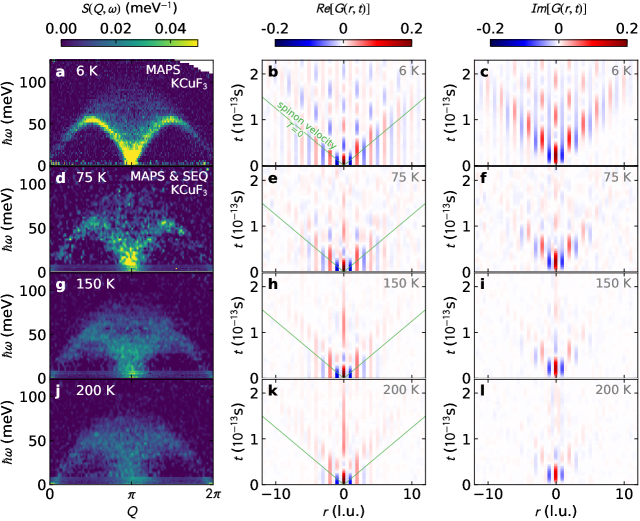
Figure 1: Scattering and Van Hove correlations. Finite temperature neutron scattering data for KCuF₃ (left column) and their transformation to real-space correlations, with the real $G(r,t)$ (center column) and imaginary $G(r,t)$ (right column). Red indicates ferromagnetic spin correlation, blue indicates antiferromagnetic spin correlation. At low temperatures, the real $G(r,t)$ wavefront at the light cone is antiferromagnetic, and by 200 K it becomes ferromagnetic. Meanwhile, the imaginary $G(r,t)$ is restricted in space and time at higher temperatures, showing loss of quantum coherence.

Experimental $G(r,t)$ results are obtained using available KCuF₃ data from Refs. Lake et al. (2013); Scheie et al. (2021b) (full details are provided in the Methods section). The result is shown in Fig. 1, where ferromagnetic $G(r,t)$ correlations are shown in red and antiferromagnetic correlations are shown in blue. To help interpret the experimental $G(r,t)$, we also calculated $G(r,t)$ from: (i) Bethe Ansatz Lake et al. (2013) for zero temperature, and (ii) semiclassical linear spin wave theory (LSWT). These are shown in Fig. 2.

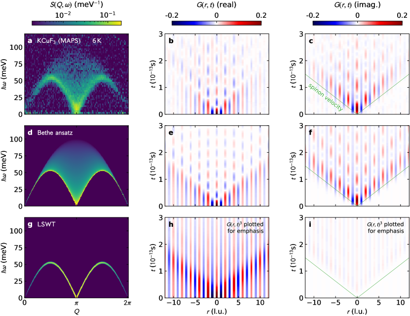
Figure 2: Van Hove time-dependent real-space spin-spin correlation compared to theory with imaginary components. a 6 K KCuF₃ scattering, b real component of $G(r,t)$, c imaginary component of $G(r,t)$. Panels d - f show the same for $T=0$ Bethe ansatz, and g - i show the same for $T=0$ LSWT on a $S=1/2$ HAF chain (renormalized by $\pi/2$ to match the light cone velocity in the top two panels). The thin green lines on $G(r,t)$ plots show the magnon/spinon velocity.

Real space $G(r,t)$ for spin systems can also be probed with cold atom and trapped ion experiments Langen et al. (2013); Cheneau et al. (2012); Jurcevic et al. (2014), but $G(r,t)$ derived from neutron scattering has several unique advantages: (i) The systems probed by neutrons are thermodynamic, and temperature is a well-defined quantity. (ii) Neutrons explore the spin system’s evolution following a local perturbation. (iii) As we show below, neutron scattering accesses the imaginary $G(r,t)$ which reveals quantum coherence and Heisenberg uncertainty.

The Fourier transform of the $S(Q,\omega)$ scattering data produces a $G(r,t)$ with complex values, with a distinct interpretation for the real and imaginary parts. As noted by Van Hove Van Hove (1954b), the imaginary part $Im[G(r,t)]=\frac{1}{2i}\langle[S_{i}^{\alpha}(0),S_{i+r}^{\alpha}(t)]\rangle$ (${\alpha}=x,y,z$) quantifies the imbalance between positive and negative energy scattering. By Robertson’s relation Robertson (1929), a nonzero commutator between observables implies Heisenberg uncertainty; thus nonzero imaginary $G(r,t)$ indicates the presence of an uncertainty relation between $S_{i}^{z}(0)$ and $S_{j}^{z}(t)$. This mutual incompatibility is thus an indicator of quantum coherence between spins (see supplemental information). It is striking that the quantum coherence can be tracked as a function of temperature with the imaginary $G(r,t)$ in Fig. 1. As temperature increases, the nonzero imaginary $G(r,t)$ shrinks to shorter and shorter times and distances, showing how the finite-temperature macroscopic world emerges from the quantum world. On the other hand, the real part $Re[G(r,t)]=\frac{1}{2}\langle\{S_{i}^{\alpha}(0),S_{i+r}^{\alpha}(t)\}\rangle$ extracts classical behaviour surviving even at infinite temperature.

The real space correlations in Figs. 1 and 2 emerge from a flipped spin at $t=0$, $r=0$. A number of things can be observed from these $G(r,t)$ data: first, the characteristic “light cone” defined by the spinon velocity $v=\frac{\pi J}{2}$ where $J$ is the exchange interaction. At low temperatures, everything below the light cone is static while everything above it is dynamic. Second, at low temperature in $G(r,t)$ there is a clear distinction between even and odd sites: the odd neighbor correlations quickly decay to zero above the light cone, whereas the even neighbor correlations persist to long times. Third, as temperature increases the spin oscillations above the light cone shrink to shorter distances and times, until by 200 K the on-site ($r=0$) correlation oscillates only once and no neighbor-site oscillations are visible. Fourth and finally, the wavefront above the light cone changes to ferromagnetic at high temperatures (Fig. 1h) whereas it was antiferromagnetic at low temperatures. This accompanies the nonzero imaginary $G(r,t)$ shrinking to shorter and shorter times and distances as temperature increases.

To gain a better understanding of the signal, we should identify which excitations are responsible for which part. The light cone is due to the low-energy correlations around $Q\sim\pi$ which can be understood from traditional bosonization, the Fermi velocity being given by the group velocity of $Q\sim\pi$ spinons. These being the fastest-moving ballistic particles, they limit the velocity of energy, correlations, and entanglement propagation, giving the Lieb-Robinson bound Lieb and Robinson (1972); Bravyi et al. (2006). Such a light cone is seen in theoretical simulations Calabrese and Cardy (2007); Bonnes et al. (2014); Collura et al. (2015); de Paula et al. (2017); Langer et al. (2011); Vlijm and Caux (2016) and cold-atom experiments Cheneau et al. (2012), and nicely also here in KCuF₃.

Letting the fast-moving ballistic particles “distill” away leaves a “quantum wake” behind the wavefront, a persistent oscillating state above the light cone which is clearly seen in Fig. 1 panel b and Fig. 2 panels b, c, e and f. This originates from another crucial characteristic of $S(Q,\omega)$, namely that its correlation weight is spread nontrivially within the spinon continuum. Contrasting LSWT with Bethe Ansatz in the second and third row of Fig. 2 shows stark differences in dephasing behaviour. LSWT, being inherently coherent, has very slow dephasing and no quantum wake. For the experimental and Bethe Ansatz $G(r,t)$ however, there exist pockets of states around $Q\sim\pi/2,\>3\pi/2$, $\omega\simeq\pi J/2$ which display a Van Hove singularity in their density of states. Since the existence and sharpness of the lower edge are contingent on integrability, measuring the (slowness of the) time decay of the quantum wake is in fact a direct experimental measurement of the proximity to integrability.

To more illustratively map the features in $G(r,t)$ with specific spinon states, we selectively remove parts of the Bethe Ansatz $S(Q,\omega)$ spectrum, keeping only key features, and Fourier transform into $G(r,t)$. As shown in Fig. 3(a)-(b), the oscillations above the light cone come from the $Q=\pi/2$ Van Hove singularities at the top of the spinon dispersion where the spinons have zero group velocity. Meanwhile, Fig. 3(c)-(d) shows the light cone emerges from the strongly dispersing low-energy $Q=\pi$ states. Combining these two states in Fig. 3(e)-(f) gives a rough reproduction of the actual $G(r,t)$, indicating that the $Q=\pi/2$ and $Q=\pi$ spinon states are what give the Heisenberg chain quantum wake its distinctive properties. Bolstering this conclusion is the analysis shown in Fig. 3(g)-(h) where we remove the oscillations above the light cone from $G(r,t)$, and transform back into $S(Q,\omega)$. In this case, we see the familiar spinon spectrum, but with the stationary $Q=\pi/2$ states missing—showing that the flat singularity at the top of the spinon dispersion is responsible for the long-lived oscillating spin correlations.

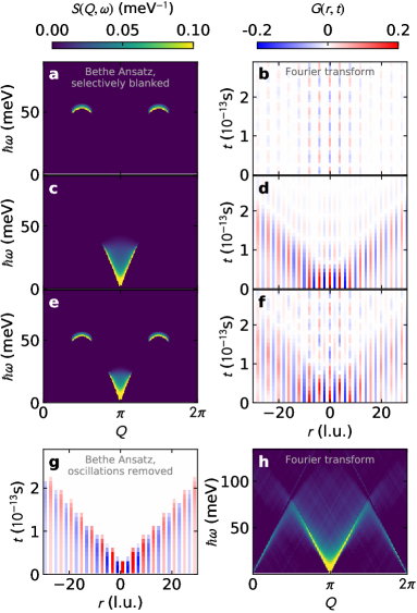
Figure 3: Signal analysis of the Bethe Ansatz. The right column is the Fourier Transform of the left. Panels (a), (c), and (e) show the Bethe Ansatz with everything removed but key features at $Q=\pi$ or $Q=\pi/2$. Panels (b), (d), and (e) show the resulting Fourier transform of these spectra into real space and time. This clearly shows that the oscillations above the light cone are due to the stationary $Q=\pi/2$ states, while the light cone is due to the dispersive $Q=\pi$ state. Panel (g) shows the $G(r,t)$ of the Bethe Ansatz with all correlations above the light cone set to zero. Fourier-transforming this back into $S(Q,\omega)$ in panel (h), we find a spinon spectrum with the $Q=\pi/2$ stationary states missing—confirming that these are responsible for the oscillating Floquet dynamics.

Quantum scrambling:

Perhaps the most striking feature of the KCuF₃ quantum wake is the total loss of Néel correlations above the light cone. Below the light cone, the system shows static $Q=\pi$ antiferromagnetism. Above the light cone, the system shows dynamic period-doubled $Q=\pi/2$ antiferromagnetism, with hardly a trace of the original state. In stark contrast to this, equal-time real space correlators $\langle S^{\alpha}_{i}(t)S^{\alpha}_{j}(t)\rangle$ (as opposed to dynamical correlator $G(r,t)$ which measures $\langle S^{\alpha}_{i}(0)S^{\alpha}_{j}(t)\rangle$) computed from Bethe ansatz show rapid reemergence of $Q=\pi$ antiferromagnetism above the light cone, where nearest neighbor $\langle S^{\alpha}_{0}(t)S^{\alpha}_{1}(t)\rangle\rightarrow\frac{1}{12}-\frac{\ln 2}{3}\simeq-0.1477...$  Hulthén (1938) as $t\rightarrow\infty$. At first glance, these results are contradictory; but the difference between $\langle S^{\alpha}_{0}(0)S^{\alpha}_{1}(t)\rangle$ and $\langle S^{\alpha}_{0}(t)S^{\alpha}_{1}(t)\rangle$ indicates the new AFM correlations form in a basis orthogonal to the original basis. In other words, the $t\rightarrow\infty$ state has zero correlations with the $t=0$ state, in accord with Anderson’s orthogonality catastrophe Anderson (1967).

This process can be more precisely described as quantum scrambling: the delocalization of quantum information over time Luitz and Bar Lev (2017); Swingle (2018). Typically such physics is studied via out of time order correlators (OTOC—see Supplemental Materials section for details). $G(r,t)$ provides an alternative and more experimentally accessible way to study quantum scrambling, quench dynamics, and quantum thermalization in physical systems.

Heuristic understanding of $G(r,t)$:

The $\pi/2$ oscillations inside the quantum wake can be understood heuristically as particle-antiparticle annihilation. In an antiferromagnetic chain, a down spin flipped up creates two spinons, while an up spin flipped down creates two antispinons. These quasiparticles interfere as schematically shown in Fig. 4. Spinons from even neighbor sites interfere constructively and produce a full spin flip, while antispinons from odd neighbor sites interfere destructively and annihilate. Thus $G(r,t)$ oscillates on even sites and $Re[G(r,t)]=0$ on odd sites.

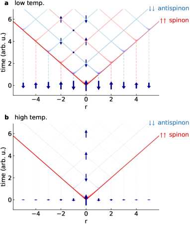
Figure 4: Schematic description of the AFM Van Hove correlations. At low temperatures, (a) a central spinon light cone emanates from $r=0$, $t=0$. As it reaches each neighboring site, it excites a pair of spinons which creates its own light cone. Odd neighbor sites have opposite spin from $r=0$ at $t=0$, and thus they create antispinon pairs. For even $r$, these spinon light cones create constructive interference and continue to flip spins up and down. For odd $r$, the spinons and antispinons destructively interfere, such that the correlations quickly go to zero. At high temperatures (b), the spin correlations are much weaker, such that the spinon and antispinon light cones emanating from $|r|>0$ are weakly coherent with $r=0$ and thus their influence is suppressed, leading to oscillations restricted in both space in time as seen in Fig. 1.

This spinon heuristic interpretation can explain the temperature evolution of $G(r,t)$ in KCuF₃. As temperature increases, the static spin correlations and spin entanglement are suppressed Scheie et al. (2021a), which destroys the coherence of the spinons from neighboring sites as illustrated in Fig. 4(b), and the oscillations vanish.

This also explains the shift to a ferromagnetic wavefront at high temperatures [Fig. 1(h)]. At low temperatures, the spinons propagate atop a substrate of antiferromagnetic correlations, giving rise to antiferromagnetic oscillating interference patterns. At higher temperatures, the static correlations are mostly gone and so are coherence with neighboring sites (evidenced by the vanishing $Im[G(r,t)]$), so the propagating spinons simply appear as a pair of up-spins hopping through the lattice. In this way, the high temperature quantum wake directly shows spinon quasiparticles—one can “see” them in the data. It is striking that a diffuse high-temperature $S(Q,\omega)$ could yield such a clear quasiparticle signature in $G(r,t)$. This technique could have profound implications for identifying exotic quasiparticles in other magnetic systems.

Conclusions:

In conclusion, we have shown using KCuF₃ scattering that it is possible to resolve real-time spin dynamics of a local quantum quench via neutron scattering. This reveals details about the quantum dynamics which were not obvious otherwise. First, we are able to directly observe the formation of an orthogonal state within the quantum wake as the light cone scrambles the initial state, leaving behind decaying period-doubled $\pi/2$ oscillations. Second, using the imaginary $G(r,t)$ we observe quantum coherence as revealed by non-commuting observables between spins more than 10 neighbors distant in Fig. 2. This is far longer range “quantumness” than is revealed by entanglement witnesses Scheie et al. (2021a). Third, the high-temperature $G(r,t)$ shows the spinon quasiparticles visually in the data, without need for theoretical models. Such details are difficult or impossible to see with other techniques.

The ability to probe short time and space dynamics of quasiparticles is of key importance to both fundamental quantum mechanics research and technological applications. On the fundamental side, the existence of a quantum wake with quasiperiodic $\pi/2$ oscillations shows behavior not captured by bosonization, which means theorists need to re-tool their analytic methods to understand the short-time dynamics of quantum spin chains. Also, measuring $G(r,t)$ at a well-defined finite temperature may shed light on eigenstate thermalization and quantum scrambling in higher-dimensional systems. On the applications side, $G(r,t)$ is more closely related to the output of current quantum computers and so may provide more direct application of this technology. Also, understanding the short-time behavior of quasiparticles in quantum systems is a crucial step in using them for quantum logic operations in real technologies. Neutron scattering derived $G(r,t)$ provides key insight into these problems.

Methods

Full methods are available in the Supplementary Information.

Extracting $G(r,t)$ from inelastic neutron scattering

The high-energy scattering data was measured on MAPS at ISIS with phonons subtracted, and low energy ($<7$ meV) scattering data at high temperatures—where the MAPS data is noisy—was filled in with data measured on SEQUOIA Granroth et al. (2006) at ORNL’s SNS Mason et al. (2006). Both data sets were corrected for the magnetic form factor, and the resulting combined data are shown in Fig. 1.

We then masked the elastic scattering (as it is mostly nonmagnetic incoherent scattering), calculated the negative energy transfer scattering using detailed balance, and computed the Fourier transform of the neutron scattering data in both $Q$ and $\hbar\omega$, yielding spin-spin correlation in real space and time $G(r,t)=\langle S(0)\cdot S_{r}(t)\rangle$. (Prior to transforming, the high energy MAPS data was interpolated using Astropy Gaussian interpolation Astropy Collaboration (2018) to create a uniform grid.)

The short-distance long-time $G(r,t)$ dynamics are governed by the lowest measured energies. In this case, the low energy cutoff was $0.7$ meV which means $G(r,t)$ is reliable only up to $\sim 5\times 10^{-13}$ s. Further details are given in the Supplemental Information. Thus, the long-time dynamics are inaccessible to the current data set. This being said, there is an important visible difference between KCuF₃ and the Bethe Ansatz $G(r,t)$ at long times: KCuF₃ tends toward antiferromagnetic correlations (odd neighbors fade towards red, even neighbors fade more blue), whereas the Bethe ansatz shows no such trend. This is because KCuF₃ is magnetically ordered at 6 K due to interchain couplings, and thus has an infinite-time static magnetic pattern; but the idealized 1D Heisenberg AFM does not. Remarkably, the Van Hove function picks this up even though the elastic line—and thus the Bragg intensity—was not included in the transform.

Theoretical simulations

The Bethe Ansatz plots were produced from data obtained using the ABACUS algorithm Caux (2009) which computes dynamical spin-spin correlation function of integrable models through explicit summation of intermediate state contributions as computed from (algebraic) Bethe Ansatz. Linear spin wave calculations were carried out using SpinW Toth and Lake (2015).

In the Supplemental Information, we also consider (i) the $S=1/2$ ferromagnet using both density matrix renormalization group theory (DMRG) and LSWT, and (ii) the quantum $S=1/2$ Ising spin chain for various anisotropies using perturbation theory.

Supplemental Information for Quantum wake dynamics in Heisenberg antiferromagnetic chains

I Real and imaginary $G(r,t)$

As noted in the main text, the real and imaginary parts of $G(r,t)$ probe different quantum mechanical functions. The imaginary $G(r,t)$ is written

$$Im[G(r,t)]=\frac{1}{2i}\big{[}\langle S_{i}^{z}(0)S_{j}^{z}(t)\rangle-\langle S_{i}^{z}(0)S_{j}^{z}(t)\rangle^{*}\big{]}$$ (S.1)

$$=\frac{1}{2i}\langle S_{i}^{z}(0)S_{j}^{z}(t)-S_{j}^{z}(t)S_{i}^{z}(0)\rangle$$

which can be written with a commutator

$$Im[G(r,t)]=\frac{1}{2i}\langle[S_{i}^{z}(0),S_{j}^{z}(t)]\rangle$$ (S.2)

Therefore, the imaginary component of $G(r,t)$ directly gives the dissipative susceptibility. Following the same derivation, we arrive at the equation for the real part of $G(r,t)$

$$Re[G(r,t)]=\frac{1}{2}\langle\{S_{i}^{z}(0),S_{j}^{z}(t)\}\rangle.$$ (S.3)

Comparing eq. (S.2) and eq. (S.3), one can see why the imaginary part of $G(r,t)$ goes to zero at infinite temperature or in the classical limit: as all states are equally populated, the commutator (and thus dissipations) vanish. This corresponds to $\mathcal{S}(-q,-\omega)=\mathcal{S}(q,\omega)$. Meanwhile, so long as correlations exist, eq. (S.3) is nonzero even at infinite temperature or in the classical limit.

A nonzero commutator between spins has a non-trivial relationship to quantum entanglement. Generically, the equal time spin operators of any two different spins always commute: $[S_{i}^{\alpha}(0),S_{j}^{\beta}(0)]=0$, no matter whether the wavefunction formed by the two spins has off-diagonal density matrix components (i.e., no matter whether the two spins are entangled). To obtain a nonzero commutator (and thus an uncertainty relation), one must introduce time evolution to one of the spins with a Hamiltonian that involves interaction between $S_{i}$ and $S_{j}$. In this case, the commutator may be nonzero.

The presence of Heisenberg uncertainty generically implies quantum coherence between two operators, such that an observation of one quantity destroys the other’s state. This is actually the opposite of quantum entanglement, where observation of one quantity determines the other’s state. Thus, the presence of nonzero imaginary $G(r,t)$ does not necessarily imply quantum entanglement (defined by off-diagonal density matrix components), but instead it witnesses a quantum coherence between $S_{i}$ and $S_{j}$. This is related (but not formally equivalent to) quantum discord, which is a generic measure of quantum correlations Ollivier and Zurek (2001); Luo (2008). Thus $Im[G(r,t)]$ is a witness of the quantum coherence of a system, which in the case of KCuF₃ extends to beyond 10 neighbors along the chain at 6 K. This is in accord with its highly coherent and entangled ground state. As temperature increases, the imaginary $G(r,t)$ becomes severely truncated in space, as shown in the main text Fig. 1.

II Ferromagnetic spin chain

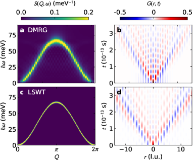
Figure S1: Real space spin correlations for a 1D Heisenberg ferromagnetic $S=1/2$ chain at $T=0$, simulated with DMRG and LSWT. Simulated neutron spectra are shown on the left, and Van Hove spin correlations (real part) are on the right. In this case, the semiclassical LSWT spin correlations are close to the DMRG quantum calculations, but the DMRG shows more oscillations near $r=0$ at long times.

As discussed in the main text, the $\pi/2$ stationary oscillations inside the quantum wake can be understood heuristically as spinon-antispinon interference. Here we propose an alternative (equally valid) heuristic for understanding the $\pi/2$ oscillations within the quantum wake: the effects of a spin-down operator on a down spin. If the $t=0,r=0$ spin is flipped up-to-down and the down-spin spinon propagates outward, the spin-lowering operator acting on a down spin results in zero. Meanwhile, the spin-lowering operator acting on an up-spin results in a spin flip. Thus odd (up-spin) sites correlations go to zero as the spinon light cone passes, and even sites flip.

To confirm the validity of these spinon heuristics, we also consider the isotropic $S=1/2$ ferromagnetic chain, and simulate its $T=0$ neutron spectra with DMRG White (1992, 1993); Alvarez (2009) and LSWT, see Fig. S1. The DMRG calculation was performed on a chain of $L=50$ sites with open boundaries, keeping up to $m=500$ states in the calculation. $S(Q,\omega)$ was calculated using the DMRG++ Alvarez (2009) implementation of the Krylov-space correction vector method Kühner and White (1999); Nocera and Alvarez (2016), and a Lorentzian energy broadening with half-width at half-maximum (HWHM) $\eta=0.1|J|$ to account for the finite-size system. To isolate the inelastic scattering, a Lorentzian with height $S(Q,0)$ was substracted at each $Q$-point.

Unlike the AFM case, excitations from the zero temperature FM ground state are spin flips of the same direction, which would mean no antiparticles are created and no destructive interference will occur. This is indeed what we see: all sites oscillate in time above the light cone, and no continuum exists in $S(Q,\omega)$.

If there were regular destructive interference, it would by necessity create a continuum in the neutron spectrum $S(Q,\omega)$: well-defined oscillations in time corresponds to a sharp mode in energy, whereas suppressed (or quickly decaying) correlations correspond to diffuse modes in energy. So even without transforming the neutron data into $S(Q,\omega)$, it should be obvious from the well-defined mode that there is no significant particle-antiparticle annihilation in $G(r,t)$ for the zero temperature FM spin chain.

III Toward the Ising limit

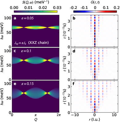
Figure S2: Simulated spin correlations for a 1D Ising AFM chain for three different values of anisotropy. Simulated $S_{xx}(Q,\omega)$ neutron spectra are shown on the left column (calculated via perturbation theory as described in Ref. Ishimura and Shiba (1980)), and Van Hove spin correlations (real part only) are on the right column. Similar to Fig. 2 in the main text, the odd neighbor sites correlations decay to zero while even neighbor sites oscillate to long times. The “light cone” gets steeper and steeper as the Ising limit is approached.

Figure S2 shows the calculated real space correlations from perturbation theory at $T=0$ approaching the Ising limit. The $S(q,\omega)$ was calculated as described in Ref. Ishimura and Shiba (1980) and transformed into $G(r,t)$. There are several things worth noting: first, just like the $S=1/2$ Heisenberg chain, the odd neighbor sites’ correlations go to zero, in accord with spinon-antispinon interference. Second, there is no well-defined wavefront visible in the data—possibly because the simulated intensity only includes the inelastic channel. Finally, as the Ising limit is approached, the “light cone” gets steeper and steeper, corresponding to slower and slower spinon velocities.

IV The XY limit

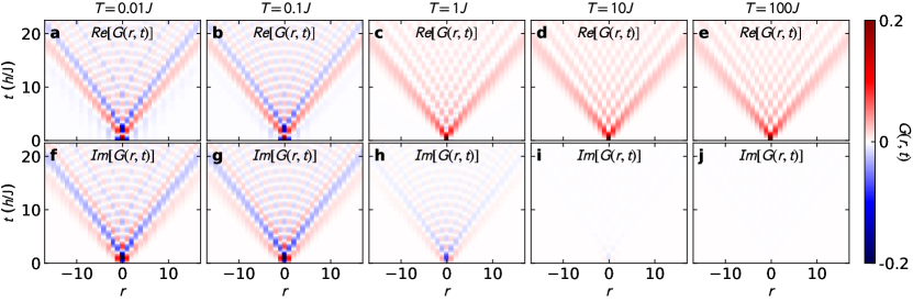
Figure S3: Real (top row) and imaginary (bottom row) part of $\left\langle S_{j}^{z}(t)S_{l}^{z}(0)\right\rangle$ for the XX model, Eq. (S.5), as a function of temperature. The real part becomes non-negative as $T$ increases, whereas the imaginary part vanishes. In addition, we see a lightcone with similarly oscillatory behavior as in the Heisenberg model.

Although the isotropic Heisenberg chain model applicable to KCuF₃ can be solved exactly using the Bethe ansatz, the resulting expressions are often complicated. We can instead consider the antiferromagnetic isotropic XY-model (or XX-model) Lieb et al. (1961),

$$\mathcal{H}=J\sum_{i=1}^{N}\left[S_{i}^{x}S_{i+1}^{x}+S_{i}^{y}S_{i+1}^{y}\right],$$ (S.4)

for which simpler, closed-form expressions can be obtained using the Jordan-Wigner formalism. At zero magnetic field, for a chain of $N$ sites with open boundary conditions, the longitudinal dynamical correlation between two lattice sites $j$ and $l$ can be written Gonçalves and Cruz (1980); Cruz and Gonçalves (1981)

$$\left\langle S_{j}^{z}(t)S_{l}^{z}(0)\right\rangle =\frac{1}{\left(N+1\right)^{2}}\left[\sum_{k}\left(\sin^{2}\left(kj\right)\right)\tanh\left(\frac{J\cos k}{2k_{B}T}\right)\right]\times\left[\sum_{k}\left(\sin^{2}\left(kl\right)\right)\tanh\left(\frac{J\cos k}{2k_{B}T}\right)\right]$$

$$+\frac{1}{\left(N+1\right)^{2}}\left(\left[\sum_{k}\sin\left(kj\right)\sin\left(kl\right)\left\{\cos\left(tJ\cos k\right)-i\sin\left(tJ\cos k\right)\tanh\left(\frac{J\cos k}{2k_{B}T}\right)\right\}\right]^{2}\right)$$

$$-\frac{1}{\left(N+1\right)^{2}}\left(\left[\sum_{k}\sin\left(kj\right)\sin\left(kl\right)\left\{i\sin\left(tJ\cos k\right)-\cos\left(tJ\cos k\right)\tanh\left(\frac{J\cos k}{2k_{B}T}\right)\right\}\right]^{2}\right),$$ (S.5)

where $k=\frac{m\pi}{N+1},\quad 1\leq m\leq N+1$, is the momentum. Due to their simple structure, these sums can be evaluated at arbitrary times, temperatures and finite sizes. Yet they still capture several of the qualitative features observed in the KCuF₃ $G(r,t)$, as shown in Fig. S3. It is easy to analytically see the emergence of real-valued ferromagnetic correlations for all times $t$ by considering the high-temperature limit of Eq. (S.5), where the $\tanh$ factors vanish, leaving

$$\left\langle S_{j}^{z}(t)S_{l}^{z}(0)\right\rangle \approx\frac{1}{\left(N+1\right)^{2}}\left(\left[\sum_{k}\sin\left(kj\right)\sin\left(kl\right)\left\{\cos\left(tJ\cos k\right)\right\}\right]^{2}+\left[\sum_{k}\sin\left(kj\right)\sin\left(kl\right)\left\{\sin\left(tJ\cos k\right)\right\}\right]^{2}\right),$$ (S.6)

which is manifestly real and non-negative for all times $t$. In the thermodynamic limit we have the expressions Gonçalves and Cruz (1980),

$$\left\langle S_{j}^{z}(t)S_{l}^{z}(0)\right\rangle =\left\{\begin{array}[]{cc}\frac{1}{4}\left[J_{j-l}\left(Jt\right)-\left(-1\right)^{l}J_{j+l}\left(Jt\right)\right]^{2},&\quad\,\text{for }T=\infty,\\ \frac{1}{4}\left[F_{j-l}\left(Jt\right)-\left(-1\right)^{l}F_{j+l}\left(Jt\right)\right]^{2},&\quad\text{for }T=0,\end{array}\right.$$ (S.9)

where $J_{n}$ is the $n$th Bessel function of the first kind and $F_{n}=J_{n}+iE_{n}$, where $E_{n}$ is the Weber function.

V Time-limit of reliability

The long time dynamics of a Fourier transform is determined by the lowest frequencies. Consequently, the reliability of the calculated $G(r,t)$ at long times is governed by the lowest measured energy. In this case, the low-energy cutoff from the SEQUOIA experiment was 0.7 meV, which yields a cutoff in time of $\frac{h}{\hbar\omega}=6\times 10^{-12}$ s, where $h$ is Planck’s constant. However, the boundary between the MAPS and SEQUOIA data is 7 meV, which yields a slight artifact in the data and causes the $G(r,t)$ to “ring” with a period $\frac{h}{\hbar\omega}=6\times 10^{-13}$ s—this behavior is an artifact and is not physical. When the calculations are safely below this threshold, the $G(r,t)$ is reliable, as shown in Fig. S4. Although the lower energy SEQ data produced this ringing, we found that it was necessary to include in order to get a clean Fourier transform signal at higher temperatures.

To be completely safe from ringing effects, we find that one needs to stay below half the cutoff time ($3\times 10^{-13}$ s for this experiment). Thus, any experiments aiming to measure $G(r,t)$ to long times must measure to appropriately high resolution and low energies.

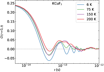
Figure S4: On-site correlation $r=0$ for KCuF₃ at various temperatures, showing the oscillations decaying. Beyond $4\times 10^{-13}$ s, the results are not reliable and the “ringing” from the low-energy cutoff begins to dominate the signal.

VI Quantum scrambling and out of time correlators

Quantum scrambling is typically studied using out of time order correlators (OTOC) Maldacena et al. (2016); Swingle (2018); Gärttner et al. (2017); Li et al. (2017); Luitz and Bar Lev (2017); Colmenarez and Luitz (2020), which in spin chains are defined as

$$F(t)=\langle\hat{S}_{a}^{\dagger}(t)\hat{S}_{b}^{\dagger}\hat{S}_{a}(t)\hat{S}_{b}\rangle$$ (S.10)

where $\hat{S}_{a}(t)$ and $\hat{S}_{b}$ are two different spin operators at time $t$ and $t=0$ respectively. The OTOC is related to the commutator between these operators $Re[F(t)]=1-\langle|[\hat{S}_{a}(t),\hat{S}_{b}]|^{2}\rangle/2$, which functionally makes the OTOC a measure of how $\hat{S}_{a}(t)$ and $\hat{S}_{b}$ fail to commute Gärttner et al. (2017). In 1D spin chains, OTOCs reveal quantum scrambling above the light cone Nakamura et al. (2019); Luitz and Bar Lev (2017); Kim and Huse (2013). This is similar (but not identical) to imaginary $G(r,t)$, which also measures $[\hat{S}_{a}(t),\hat{S}_{b}]$ (Eq. S.2), and thus provides similar information.

As shown in Fig. LABEL:fig:hightemp_imag and Fig. 2 of the main text, imaginary $G(r,t)$ correlations are only nonzero above the light cone, in good agreement to the commuting spin operators in the Heisenberg antiferromagnetic ground state. Above the light cone, both Bethe ansatz and KCuF₃ show nonzero negative static $\mathrm{Im}[G(r,t)]$ on the odd sites, and oscillating but average positive $\mathrm{Im}[G(r,t)]$ on the even sites. This concurs with quantum scrambling, where time-like separated spin operators do not commute with the original magnetism.

References

- Heisenberg (1928) W. Heisenberg, Z. Phys. 49, 619 (1928).
- Bethe (1931) H. A. Bethe, Zeit. für Physik 71, 205 (1931).
- Faddeev and Takhtajan (1981) L. D. Faddeev and L. A. Takhtajan, Phys. Lett. A 85, 375 (1981).
- Tennant et al. (1993) D. A. Tennant, T. G. Perring, R. A. Cowley, and S. E. Nagler, Phys. Rev. Lett. 70, 4003 (1993).
- Lake et al. (2013) B. Lake, D. A. Tennant, J.-S. Caux, T. Barthel, U. Schollwöck, S. E. Nagler, and C. D. Frost, Phys. Rev. Lett. 111, 137205 (2013).
- Lake et al. (2005) B. Lake, D. A. Tennant, and S. E. Nagler, Phys. Rev. B 71, 134412 (2005).
- Scheie et al. (2021a) A. Scheie, P. Laurell, A. M. Samarakoon, B. Lake, S. E. Nagler, G. E. Granroth, S. Okamoto, G. Alvarez, and D. A. Tennant, Phys. Rev. B 103, 224434 (2021a).
- Brockhouse (1957) B. N. Brockhouse, Phys. Rev. 106, 859 (1957).
- Squires (2012) G. L. Squires, Introduction to the Theory of Thermal Neutron Scattering, 3rd ed. (Cambridge University Press, Cambridge, UK, 2012).
- Van Hove (1954a) L. Van Hove, Phys. Rev. 95, 249 (1954a).
- Van Hove (1954b) L. Van Hove, Phys. Rev. 95, 1374 (1954b).
- Brockhouse and Pope (1959) B. N. Brockhouse and N. K. Pope, Phys. Rev. Lett. 3, 259 (1959).
- Iwashita et al. (2017) T. Iwashita, B. Wu, W.-R. Chen, S. Tsutsui, A. Q. R. Baron, and T. Egami, Science Advances 3 (2017), 10.1126/sciadv.1603079.
- Giamarchi (2004) T. Giamarchi, Quantum Physics in One Dimension (Oxford University Press, 2004).
- Haldane (1981) F. D. M. Haldane, J. Phys C: Sol. St. Phys. 14, 2585 (1981).
- Lieb and Robinson (1972) E. H. Lieb and D. W. Robinson, in Statistical mechanics (Springer, 1972) pp. 425–431.
- Imambekov et al. (2012) A. Imambekov, T. L. Schmidt, and L. I. Glazman, Rev. Mod. Phys. 84, 1253 (2012).
- Scheie et al. (2021b) A. Scheie, N. E. Sherman, M. Dupont, S. E. Nagler, M. B. Stone, G. E. Granroth, J. E. Moore, and D. A. Tennant, Nature Physics (2021b), 10.1038/s41567-021-01191-6.
- Langen et al. (2013) T. Langen, R. Geiger, M. Kuhnert, B. Rauer, and J. Schmiedmayer, Nature Physics 9, 640 (2013).
- Cheneau et al. (2012) M. Cheneau, P. Barmettler, D. Poletti, M. Endres, P. Schauß, T. Fukuhara, C. Gross, I. Bloch, C. Kollath, and S. Kuhr, Nature 481, 484 (2012).
- Jurcevic et al. (2014) P. Jurcevic, B. P. Lanyon, P. Hauke, C. Hempel, P. Zoller, R. Blatt, and C. F. Roos, Nature 511, 202 (2014).
- Robertson (1929) H. P. Robertson, Phys. Rev. 34, 163 (1929).
- Bravyi et al. (2006) S. Bravyi, M. B. Hastings, and F. Verstraete, Phys. Rev. Lett. 97, 050401 (2006).
- Calabrese and Cardy (2007) P. Calabrese and J. Cardy, Journal of Statistical Mechanics: Theory and Experiment 2007, P06008 (2007).
- Bonnes et al. (2014) L. Bonnes, F. H. L. Essler, and A. M. Läuchli, Phys. Rev. Lett. 113, 187203 (2014).
- Collura et al. (2015) M. Collura, P. Calabrese, and F. H. L. Essler, Phys. Rev. B 92, 125131 (2015).
- de Paula et al. (2017) A. L. de Paula, H. Bragança, R. G. Pereira, R. C. Drumond, and M. C. O. Aguiar, Phys. Rev. B 95, 045125 (2017).
- Langer et al. (2011) S. Langer, M. Heyl, I. P. McCulloch, and F. Heidrich-Meisner, Phys. Rev. B 84, 205115 (2011).
- Vlijm and Caux (2016) R. Vlijm and J.-S. Caux, Phys. Rev. B 93, 174426 (2016).
- Hulthén (1938) L. Hulthén, Arkiv Mat. Astron. Fysik 26A, 1 (1938).
- Anderson (1967) P. W. Anderson, Phys. Rev. Lett. 18, 1049 (1967).
- Luitz and Bar Lev (2017) D. J. Luitz and Y. Bar Lev, Phys. Rev. B 96, 020406 (2017).
- Swingle (2018) B. Swingle, Nature Physics 14, 988 (2018).
- Granroth et al. (2006) G. E. Granroth, D. H. Vandergriff, and S. E. Nagler, Physica B-Condensed Matter 385-86, 1104 (2006).
- Mason et al. (2006) T. Mason, D. Abernathy, I. Anderson, J. Ankner, T. Egami, G. Ehlers, A. Ekkebus, G. Granroth, M. Hagen, K. Herwig, et al., Physica B: Condensed Matter 385, 955 (2006).
- Astropy Collaboration (2018) Astropy Collaboration, The Astronomical Journal 156, 123 (2018).
- Caux (2009) J.-S. Caux, J. Math. Phys. 50, 095214 (2009).
- Toth and Lake (2015) S. Toth and B. Lake, Journal of Physics: Condensed Matter 27, 166002 (2015).
Acknowledgments
We are thankful to Takeshi Egami for enlightening discussions. The research by P.L. was supported by the Scientific Discovery through Advanced Computing (SciDAC) program funded by the US Department of Energy, Office of Science, Advanced Scientific Computing Research and Basic Energy Sciences, Division of Materials Sciences and Engineering. This research used resources at the Spallation Neutron Source, a DOE Office of Science User Facility operated by the Oak Ridge National Laboratory. JSC acknowledges support from the European Research Council (ERC) under ERC Advanced grant 743032 DYNAMINT. The work by DAT and SEN is supported by the Quantum Science Center (QSC), a National Quantum Information Science Research Center of the U.S. Department of Energy (DOE).

References

- Ollivier and Zurek (2001) H. Ollivier and W. H. Zurek, Phys. Rev. Lett. 88, 017901 (2001).
- Luo (2008) S. Luo, Phys. Rev. A 77, 042303 (2008).
- White (1992) S. R. White, Phys. Rev. Lett. 69, 2863 (1992).
- White (1993) S. R. White, Phys. Rev. B 48, 10345 (1993).
- Alvarez (2009) G. Alvarez, Comp. Phys. Comms. 180, 1572 (2009).
- Kühner and White (1999) T. D. Kühner and S. R. White, Phys. Rev. B 60, 335 (1999).
- Nocera and Alvarez (2016) A. Nocera and G. Alvarez, Phys. Rev. E 94, 053308 (2016).
- Ishimura and Shiba (1980) N. Ishimura and H. Shiba, Progress of Theoretical Physics 63, 743 (1980).
- Lieb et al. (1961) E. Lieb, T. Schultz, and D. Mattis, Ann. Phys. (N.Y.) 16, 407 (1961).
- Gonçalves and Cruz (1980) L. Gonçalves and H. Cruz, Journal of Magnetism and Magnetic Materials 15-18, 1067 (1980).
- Cruz and Gonçalves (1981) H. B. Cruz and L. L. Gonçalves, Journal of Physics C: Solid State Physics 14, 2785 (1981).
- Maldacena et al. (2016) J. Maldacena, S. H. Shenker, and D. Stanford, Journal of High Energy Physics 2016, 1 (2016).
- Swingle (2018) B. Swingle, Nature Physics 14, 988 (2018).
- Gärttner et al. (2017) M. Gärttner, J. G. Bohnet, A. Safavi-Naini, M. L. Wall, J. J. Bollinger, and A. M. Rey, Nature Physics 13, 781 (2017).
- Li et al. (2017) J. Li, R. Fan, H. Wang, B. Ye, B. Zeng, H. Zhai, X. Peng, and J. Du, Phys. Rev. X 7, 031011 (2017).
- Luitz and Bar Lev (2017) D. J. Luitz and Y. Bar Lev, Phys. Rev. B 96, 020406 (2017).
- Colmenarez and Luitz (2020) L. Colmenarez and D. J. Luitz, Phys. Rev. Research 2, 043047 (2020).
- Nakamura et al. (2019) S. Nakamura, E. Iyoda, T. Deguchi, and T. Sagawa, Phys. Rev. B 99, 224305 (2019).
- Kim and Huse (2013) H. Kim and D. A. Huse, Phys. Rev. Lett. 111, 127205 (2013).