Implementation of polygon guarding algorithms for art gallery problems

Abstract

Victor Klee introduce the art gallery problem during a conference in Stanford in August 1976 with that question: "How many guards are required to guard an art gallery?" In 1987, Ghosh provided an approximation algorithm for vertex guards problem [4] that achieved $O(\log n)$ approximation ratio. In 2017, Bhattacharya et al. [1] presented a 6-approximation algorithm for guarding weak visibility polygons. In our paper, we first implement these algorithms and then we test them for different types of polygons. We compare their performance in terms of number of guards used by them. In the last part, we have provided a new algorithm that uses Ghosh’s idea. Experiments show that this algorithm assigns near optimal guards for guarding the input polygons.

Keywords computational geometry  $\cdot$ art-gallery  $\cdot$ approximation algorithm

1 Introduction

Victor Klee introduce the art gallery problem during a conference in Stanford in August 1976 with this question: "How many guards are required to guard an art gallery?" We describe an art gallery as a simple polygon $P$ with total of $n$ vertices. A guard can be viewed as a point in $P$. We say a point $z\in P$ is visible from a guard $g$ if the line segment $gz$ lies inside $P$ and dose not intersect the exterior of $P$. If the guards are allowed to be placed just on vertices, we called vertex guards. If there is no restriction, guards are called point guards. A polygon $P$ is called weak visibility polygon if every point in $P$ is visible from some point of edge [3].

After Victor Klee posed the art gallery problem, V. Chv´atal established in [2] that for simple polygon $P$, $\lfloor\frac{n}{3}\rfloor$ guards are always sufficient for guarding $P$. If all edge of simple polygon $P$ are vertical or horizontal, $P$ is called simple orthogonal polygon. Kahn et al. [5] and O’Rourke [7] proved that simple orthogonal polygon $P$ needs at most $\lfloor\frac{n}{4}\rfloor$ guards.

Lee and Lin [6] showed that the problem of computing a minimum number of guards for guarding a polygon is NP-Hard. In 2010, Ghosh [4] presented an approximation algorithm for minimum vertex guard problem for simple polygons. The pseudo code of algorithm is:

Algorithm 1 An $O(n^{4})$-algorithm for computing a guard set $S$ for all vertices of polygon $P$

  Draw lines through every pair of vertices of $P$ and compute all convex components $c_{1},c_{2},...,c_{m}$ of $P$

  Let $C=(c_{1},c_{2},...,c_{m})$, $N=(1,2,...,n)$ and $Q=\emptyset$

  for $j=1$ to $j=n$ do

     construct the set $F_{j}$ by adding those convex components of $P$ that are totally visible from the vertex $V_{j}$.

  end for

  while $\mid C\mid\neq\emptyset$ do

     for $j\in N$ do

        Find $i\in N$ such that $\mid F_{j}\mid\leq\mid F_{i}\mid$ and $i\neq j$

     end for

     for $j\in N$ do

        $F_{j}:=F_{j}-F_{i}$

        $C:=C-F_{i}$

     end for

  end while

In 2017, Bhattacharya et al. [1] established a 6-approximation algorithm for vertex guarding a weak visibility polygon $P$ that contains no holes and this algorithm has running time $O(n^{2})$. Its pseudo code is:

Algorithm 2 An $O(n^{2})$-algorithm for computing a guard set $S$ for all vertices of $P$

  Compute $SPT(u)$ and $SPT(v)$

  Initialize all the vertices of $P$ as unmarked

  Initialize $B\leftarrow\emptyset$, $S_{B}\leftarrow\emptyset$ and $z\leftarrow u$

  while there exists an unmarked vertex in $P$  do

     $z\leftarrow$ the first unmarked vertex on $bd_{c}(u,v)$ in clockwise order from $z$

     if every unmarked vertex of $bd_{c}(z,p_{v}(z))$ is visible from $p_{u}(z)$ or $p_{v}(z)$ then

        $B\leftarrow B\cup\left\{z\right\}$ and $S_{B}\leftarrow S_{B}\cup\left\{p_{u}(z),p_{v}(z)\right\}$

        Mark all vertices of $P$ that become visible from $p_{u}(z)$ or $p_{v}(z)$

        $z\leftarrow p_{v}(z)$

     else

        $z\prime\leftarrow$the first unmarked vertex on $bd_{c}(z,v)$ in clockwise order

        while every unmarked vertex of $bd_{c}(p_{u}(z\prime),z\prime)$ is visible from $p_{u}(z\prime)$ or $p_{v}(z\prime)$ do

           $z\leftarrow z\prime$ and $z\prime\leftarrow$ the first unmarked vertex on $bd_{c}(z\prime,v)$ in clockwise order

        end while

        $B\leftarrow B\cup\left\{z\right\}$ and $S_{B}\leftarrow S_{B}\cup\left\{p_{u}(z),p_{v}(z)\right\}$

        while there exists an unmarked vertex on $bd_{c}(u,z)$ do

           $w\leftarrow$ the first unmarked vertex on $bd_{cc}(z,u)$ in counterclockwise order

           $B\prime\leftarrow B\prime\cup\left\{w\right\}$ and $S\prime_{B}\leftarrow S\prime_{B}\cup\left\{p_{u}(w),p_{v}(w)\right\}$

           Mark all vertices of $P$ that become visible from $p_{u}(w)$ or $p_{v}(w)$

        end while

     end if

  end while

  Reinitialize all the vertices of $P$ that are visible from some guard in $S_{B}$ as unmarked

  for each vertex $z\in B\prime$ chosen in reverse order of inclusion do

     Locate and mark each unmarked vertex visible from $p_{v}(z)$ or $p_{u}(z)$

     if no new vertices get marked due to guards at $p_{v}(z)$ or $p_{u}(z)$ then

        $B\prime\leftarrow B\prime\setminus\left\{z\right\}$ and $S\prime_{B}\leftarrow S\prime_{B}\setminus\left\{p_{u}(w),p_{v}(w)\right\}$

     end if

  end for

  $B\leftarrow B\cup B\prime$

  return  the guard set $S=S_{B}$

1.1 Outline

We implement the above mentioned algorithms and test both of them on weak visibility polygons. These weak visibility polygons are generated by a procedure presented in Section 2. Further, our new algorithm is tested on simple polygons which are generated by another procedure as mentioned in Section 3. We show experimentally that this algorithm assigns near optimal guards for guarding the input polygons.

2 Test on weak visibility polygons

2.1 Algorithm for generate arbitrary weak visibility polygon

We introduce an algorithm for generating arbitrary weak visibility polygons.

Let $p=(k,0)$ and $q=(-k,0)$:

Step 1: Choose $n$ random points $x_{1},x_{2},...,x_{n}$ in $pq$ and sort them such that

$\mid px_{i}\mid>\mid px_{i+1}\mid$ for $i\in N$.

Step 2: Choose $n$ random angles $\alpha_{1},\alpha_{2},...,\alpha_{n},$ in $(0,\pi)$ and sort them such that

$\mid\alpha_{j}\mid>\mid\alpha_{j+1}\mid$ for $j\in N$.

Step 3: Choose $n$ arbitrary positive numbers $r_{1},r_{2},...,r_{n}$.

Step 4: For every $i\in N$ compute $\overrightarrow{y_{i}}$ as $\overrightarrow{y_{i}}=\overrightarrow{x_{i}}+(-r_{i}\cos\alpha_{i},-r_{i}\sin\alpha_{i})$.

Step 5: It is obvious that for every $i\in N$, a quadrilateral with vertices $x_{i}y_{i}y_{i+1}x_{i+1}$ is a convex quadrilateral so any point in this quadrilateral is visible from vertex $x_{i}$ and $y_{i}$. Choose four positive arbitrary numbers like $w_{1},w_{2},w_{3},w_{4}$ and compute $z_{i}=\frac{w_{1}x_{i}+w_{2}y_{i}+w_{3}y_{i+1}+w_{4}x_{i+1}}{w_{1}+w_{2}+w_{3}+w_{4}}$. $z_{i}$ is a point in a quadrilateral with vertices $x_{i}y_{i}y_{i+1}x_{i+1}$.

It can be seen that a polygon with vertices $qy_{1}z_{1}y_{2}z_{2}y_{3}z_{3}...y_{n-1}z_{n-1}y_{n}p$ is a weak visibility polygon. (See figure 1)

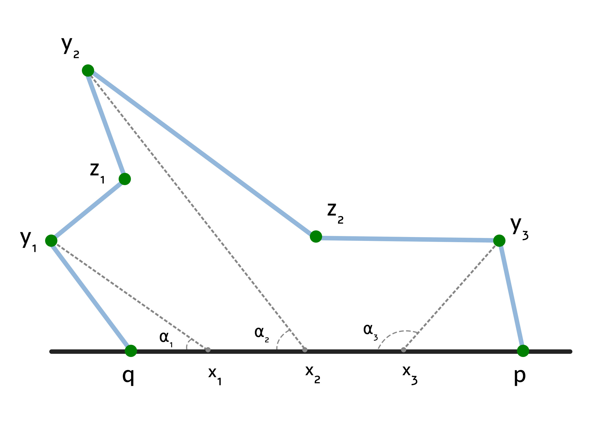
Figure 1: Generate weak visibility polygon with $n=3$.

2.2 Test on small weak visibility polygons with low value of reflex vertices

The inputs of our test are the weak visibility polygons with number of vertices $n$ are between 10 to 15 ($10\leq n\leq 15$) and number of reflex vertices $r$ are between 2 to 3 ($2\leq r\leq 3$).

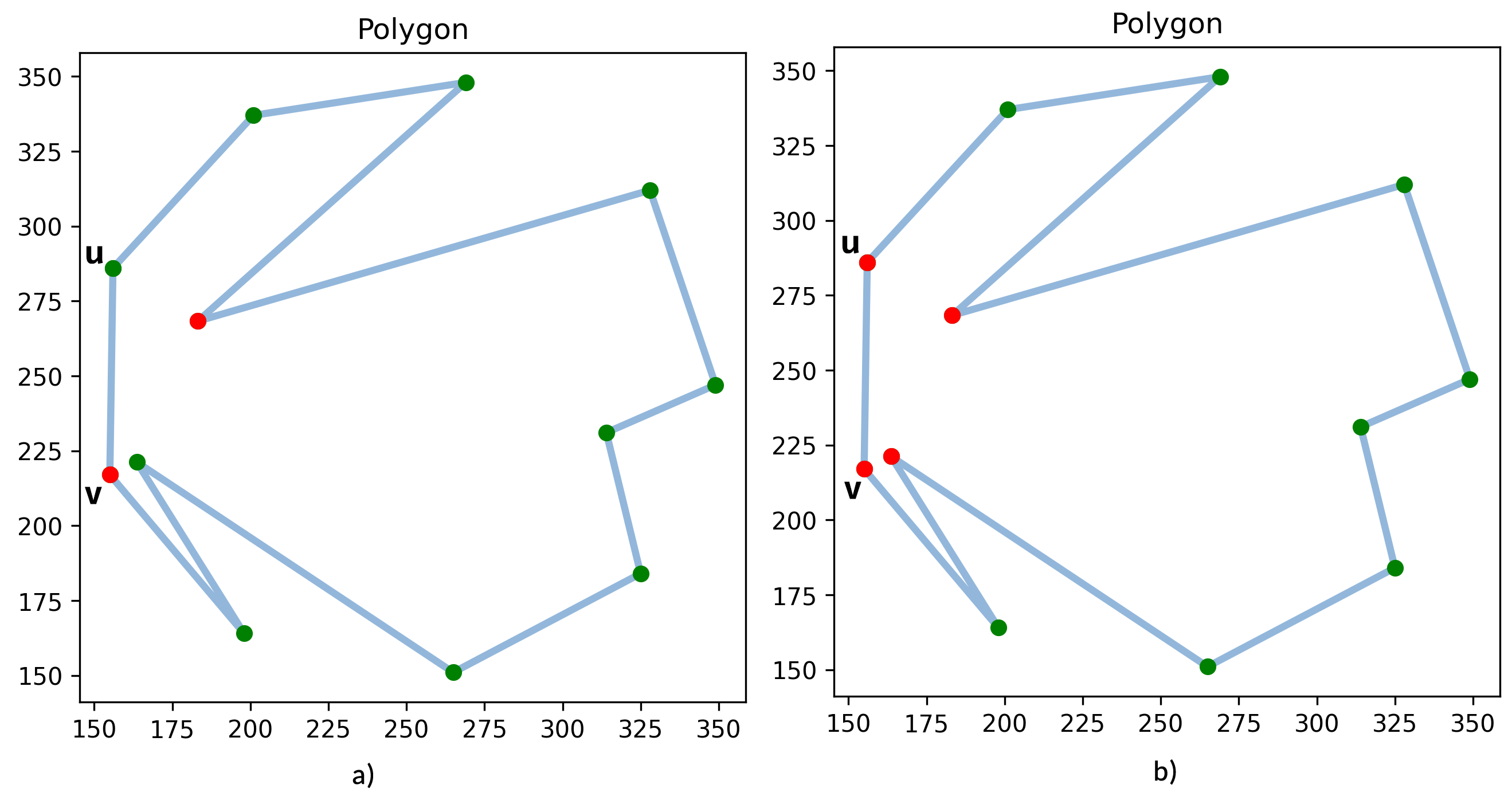
Figure 2: (a) For polygon with $12$ vertices such that $r=3$ guard set in Algorithm 1 is [(183.22, 268.31), (155.0, 217.0)] and it runs in 2.909 s. (b) guard set in Algorithm 2 is [(156.0, 286.0), (155.0, 217.0), (183.22, 268.31), (163.60, 221.22)] and it runs in 0.045 s.

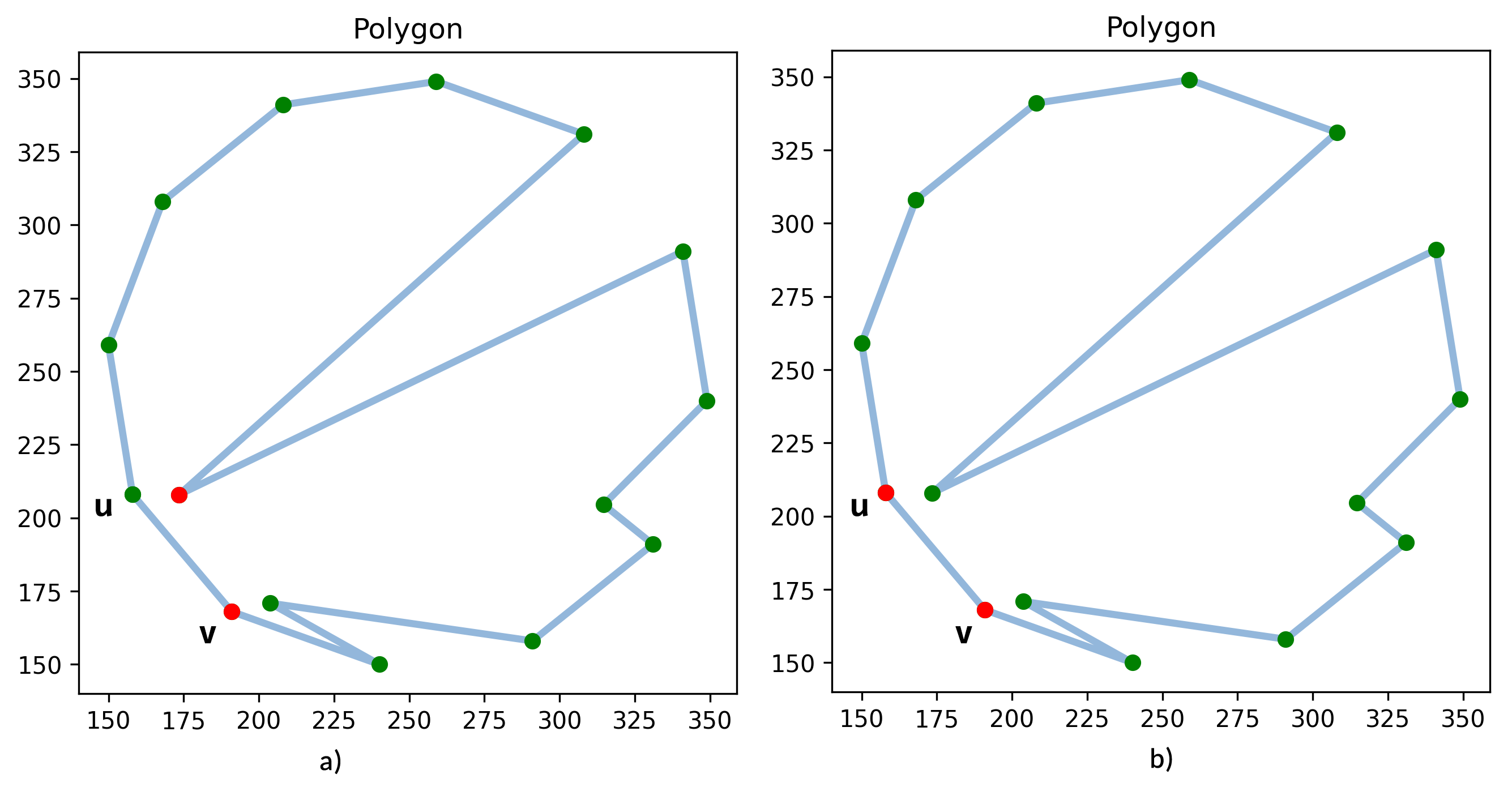
Figure 3: (a) For polygon with $15$ vertices such that $r=3$ guard set in Algorithm 1 is [(173.44, 207.91), (191.0, 168.0)] and it runs in 24.058 s. (b) Guard set in Algorithm 2 is [(158.0, 208.0), (191.0, 168.0)] and it runs in 0.0392 s.

The outputs of test suggest that (see Figure 2 and Figure 3) for a low value of $n$ and $r$, it is better to use Algorithm 1 for minimizing the number of vertex guards as Algorithm 2 uses more guards than Algorithm 1. Since Algorithm 2 is a constant approximation algorithm, Algorithm 1 performs like a constant time approximation algorithm for small values $n$ and $r$ experimentally.

Since the criteria of minimization is the number of guards rather than the running time which is an one time affair unlike online algorithms, Algorithm 1 is preferable even for weak visibility polygons.

2.3 Test on small weak visibility polygons with number of reflex vertices $r$ are roughly same and close to number of convex vertices

In this test our inputs are also weak visibility polygons with the number of vertices $n$ are between 10 to 31 ($10\leq n\leq 31$) and the number of reflex vertices $r$ are roughly same and close to number of convex vertices $(n-r)$.

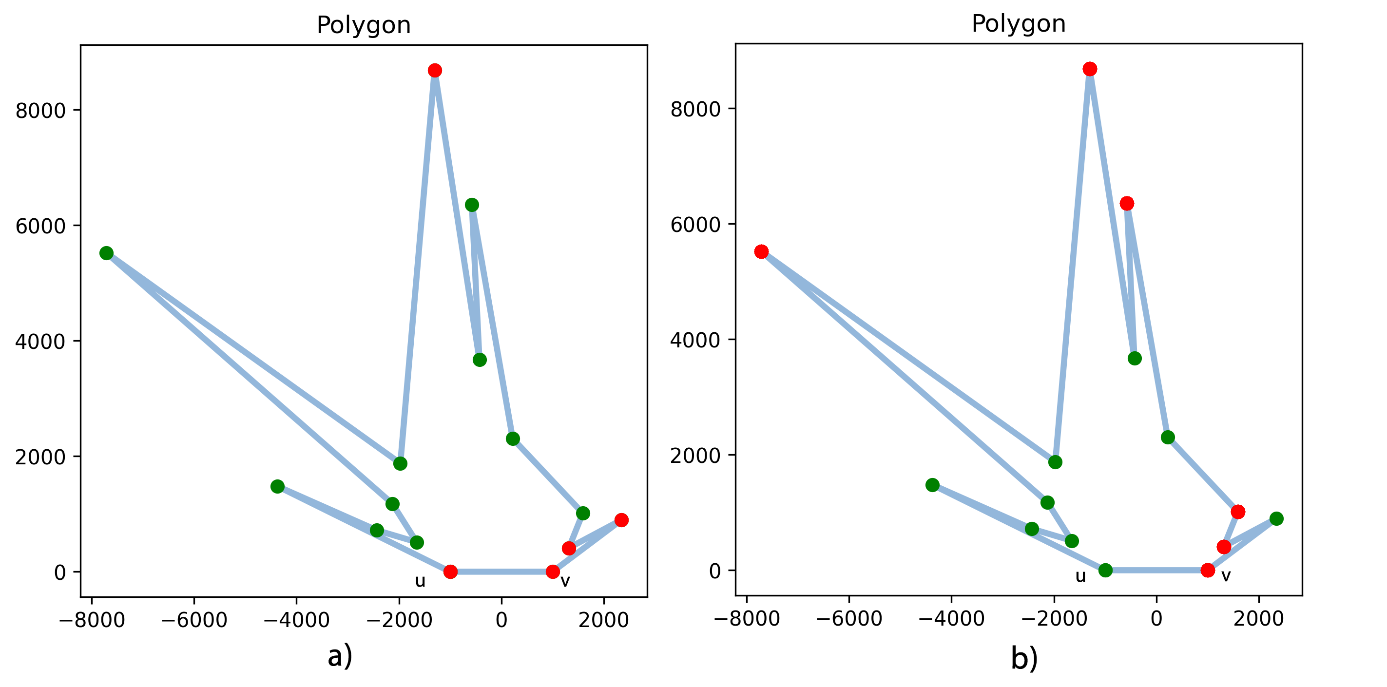
Figure 4: (a) For polygon with $15$ vertices such that $r=7$ size of guard set in Algorithm 1 is $5$ and it runs in 0.2389 s. (b) Size of guard set in Algorithm 2 is $6$ and it runs in 0.0718321 s.

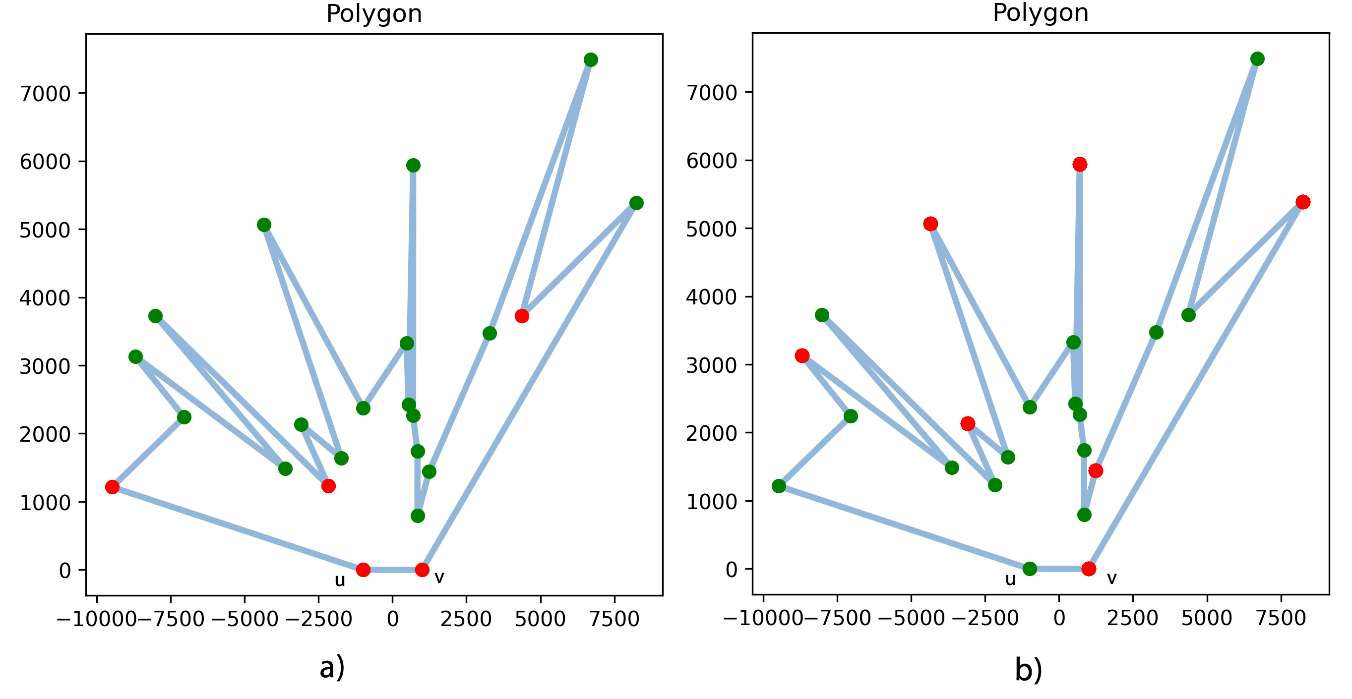
Figure 5: (a) For polygon with $23$ vertices such that $r=13$ size of guard set in Algorithm 1 is $3$ and it runs in 0.373031 s. (b) Size of guard set in Algorithm 2 is $9$ and it runs in 0.27948 s.

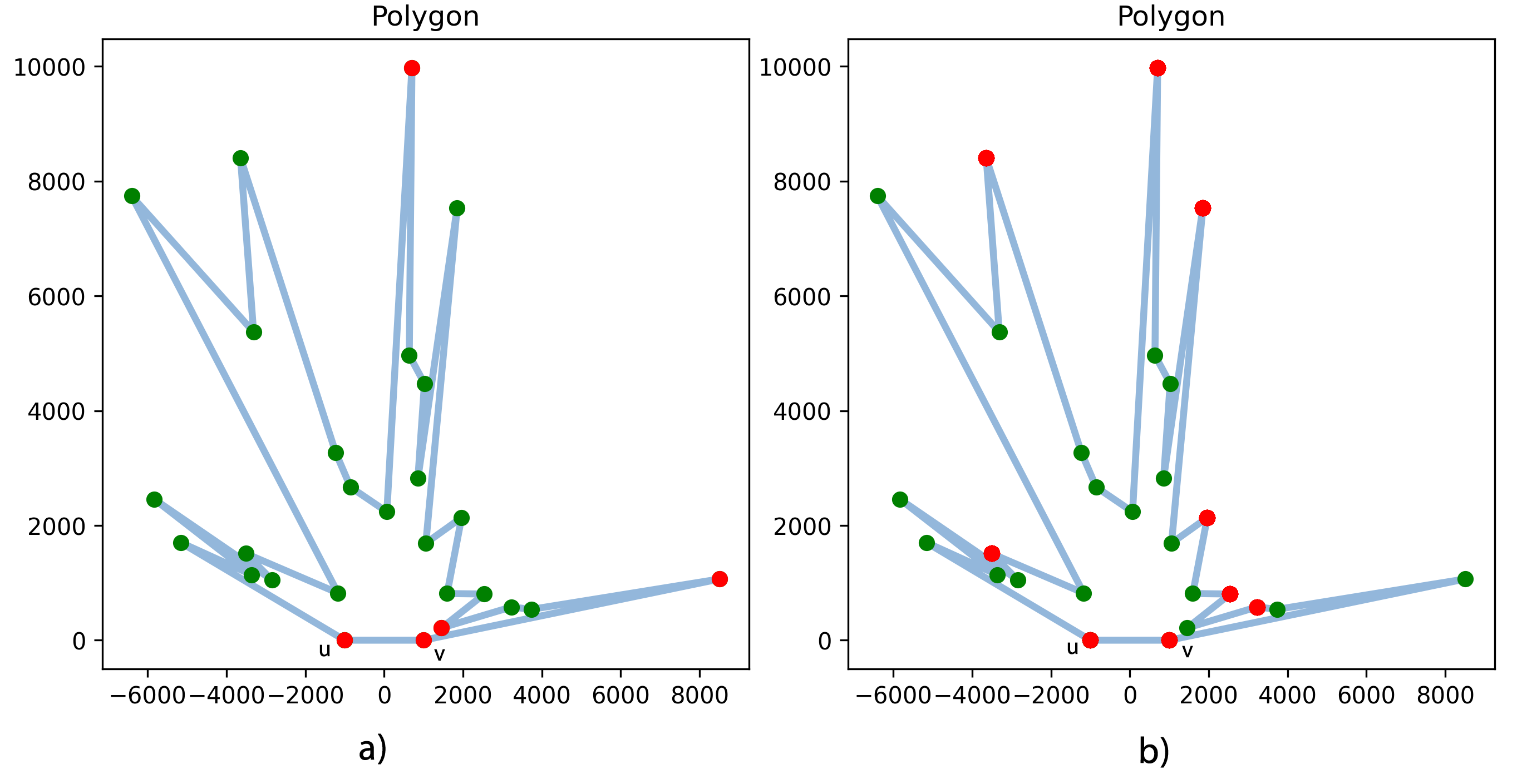
Figure 6: (a) For polygon with $27$ vertices such that $r=5$ size of guard set in Algorithm 1 is $3$ and it runs in 0.75041 s. (b) Size of guard set in Algorithm 2 is $9$ and it runs in 0.323258 s.

Based on outputs (see Figure 4, Figure 5 and Figure 6) we understand that for a low value of $n$ and $\frac{n}{2}\leq r$ Algorithm 1 is better for guarding a weak visibility polygon with minimum number of guards. because when number of reflex vertices increase, number of diameter of polygon and convex components decrease. So Algorithm 1 can be faster in this situation. Since Algorithm 1 find minimum number of guards, we prefer to use this algorithm for weak visibility polygons with low value $n$ and $\frac{n}{2}\approx r$ .

2.4 Test on large weak visibility polygons

In the last test, we test arbitrary weak visibility polygons with high value of $n$ (number of vertices) in Algorithm 1 and Algorithm 2.

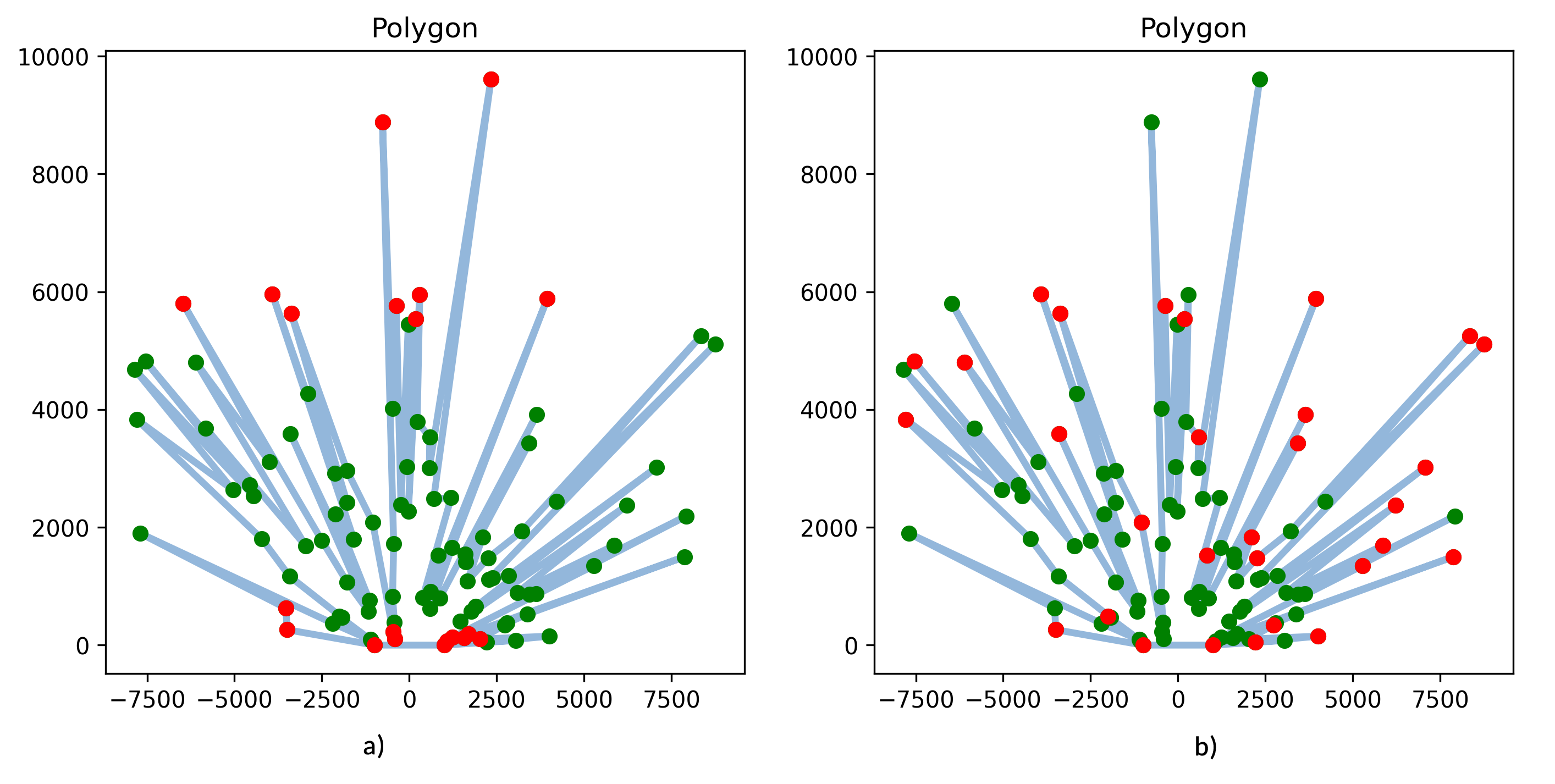
Figure 7: (a) For weak visibility polygon with $100$ vertices, Algorithm 1 uses 20 vertex guards to guard the polygon and it runs in 24.71 s. (b) For weak visibility polygon with $100$ vertices, Algorithm 2 uses 30 vertex guards to guard the polygon and it runs in 15.26 s.

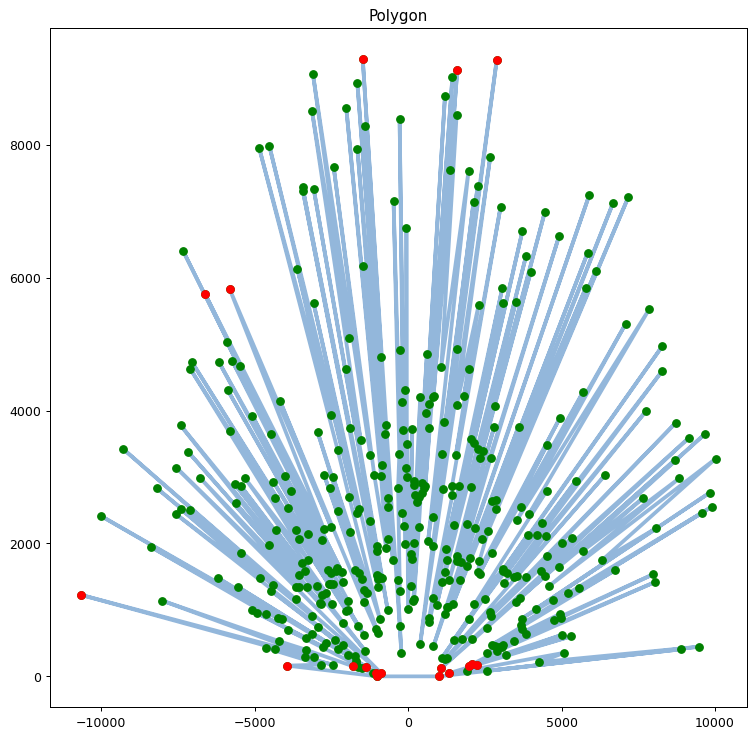
Figure 8: For weak visibility polygon with $400$ vertices, Algorithm 1 uses 18 vertex guards to guard the polygon and it runs in 231.245 s.

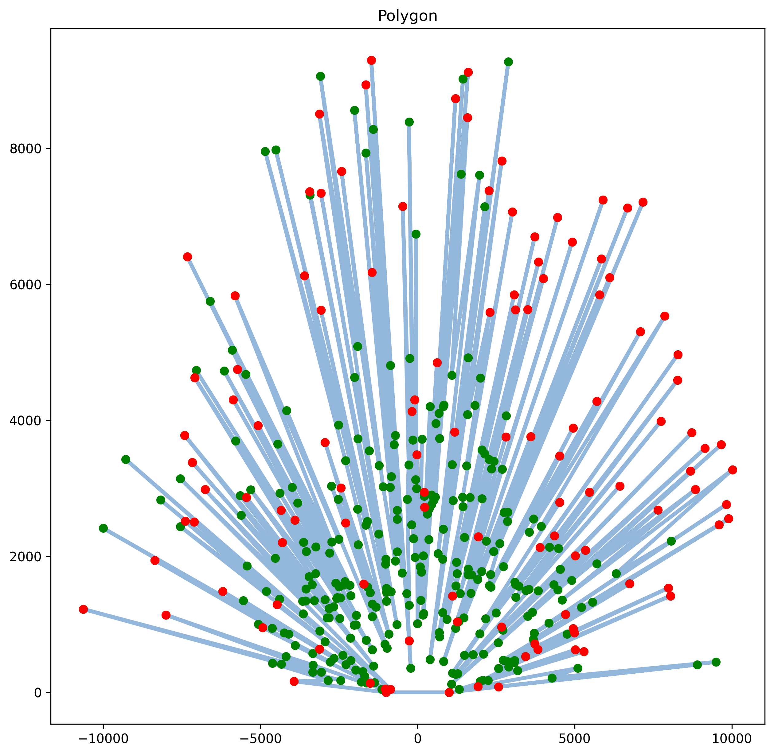
Figure 9: For weak visibility polygon with $400$ vertices, Algorithm 2 uses 115 vertex guards to guard the polygon and it runs in 199.245 s.

Based on outputs (see Figure 7, Figure 8 and Figure 9) we understand that for a high value of $n$ Algorithm 1 is better for guarding a weak visibility polygon with minimum number of guards. because Algorithm 1 use less guards than Algorithm 2 to guard a weak visibility polygon $P$.

3 Test on simple polygons

In section 2 we found out algorithm 1 assign less number of guards for weak visibility polygons that algorithm 2. Now we need to test on arbitrary simple polygon.

3.1 Algorithm for create arbitrary simple polygon

In this section we provide an algorithm that generates simple polygons with custom number of reflex vertices. the sequence of that is like :

1. Generate a simple convex polygon $P$ with $n$ number of vertices. (see Figure 10)

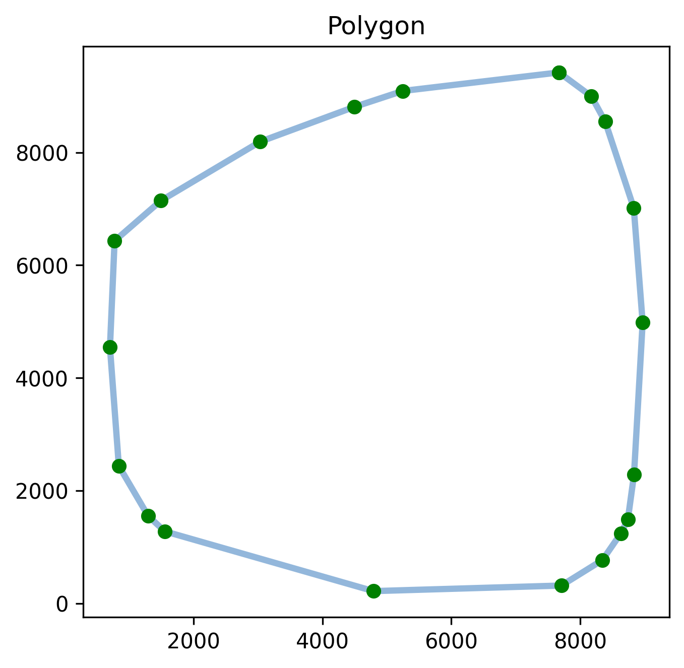
Figure 10: Generate arbitrary convex polygon

2. Triangulate $P$ such that every triangle has a joint edge with boundary of $p$.(see Figure 11)

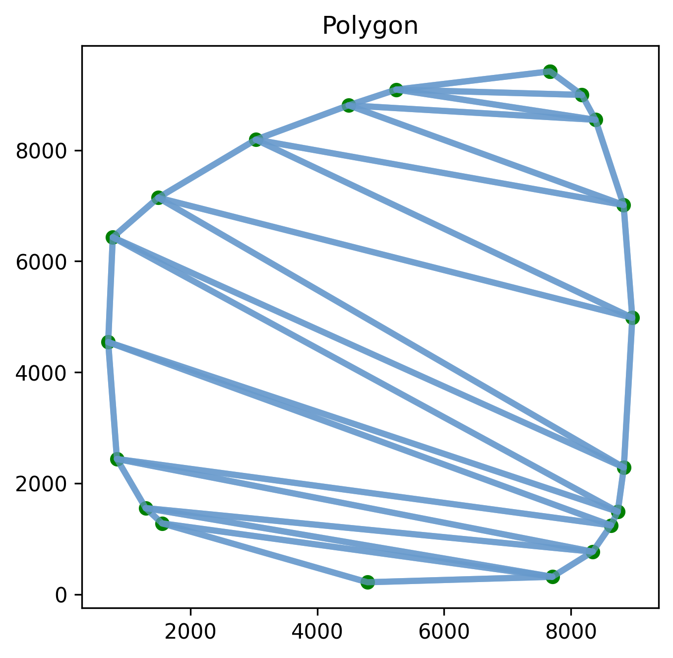
Figure 11: Example of triangulate convex simple polygon $P$.

3. Randomly add points as number of reflex vertices in $P$. (see Figure 12)

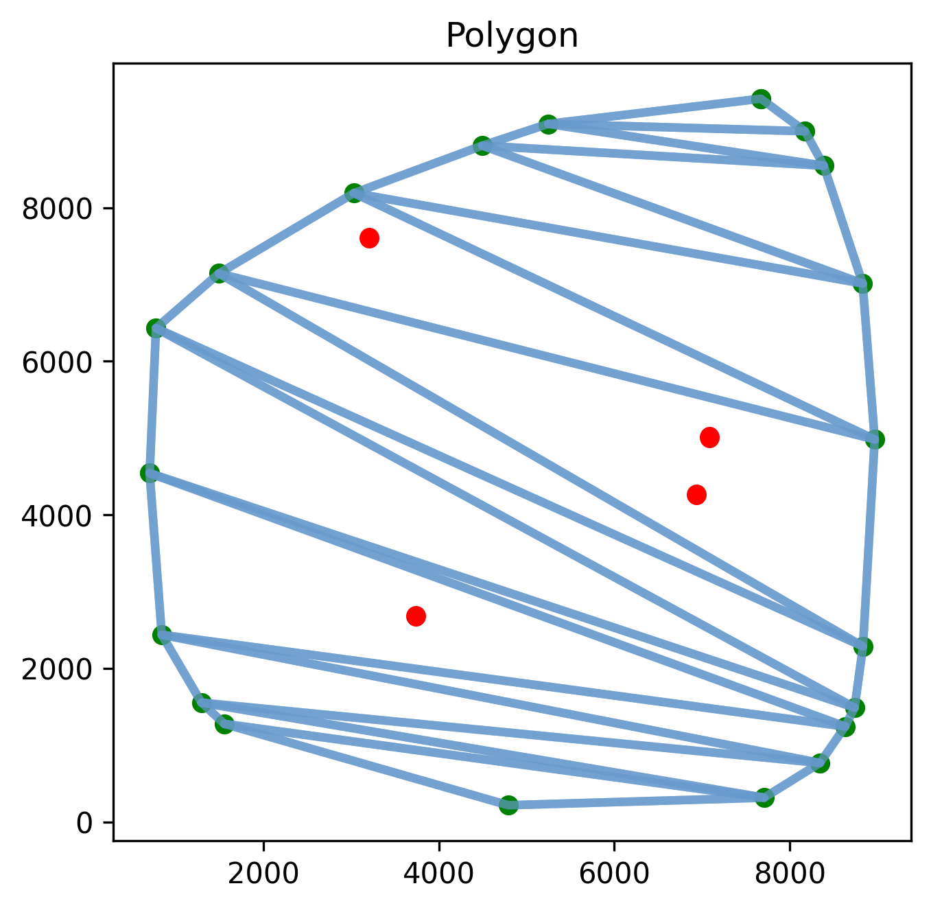
Figure 12: Generate random points in convex polygon

4. Any such added point $X$ will be inside a triangle, say $abc$. Connect $X$ to $b$ and $c$, where $b$ and $c$ are two consecutive points on the boundary of $P$. If more that one point lies inside $abc$, connect them by a simple path and then connect the endpoints of the path to $b$ and $c$. (see Figure 13)

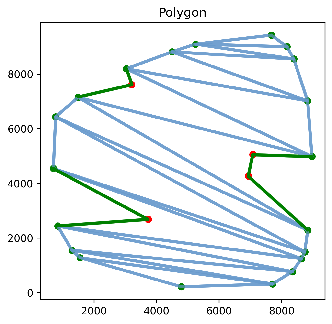
Figure 13: Connect random points to convex polygon and create arbitrary simple polygon with custom number of reflex vertices.

This method keeps our polygons simple and create custom number of reflex vertices on that.

3.2 New Algorithm for guarding

In this section we want to established an algorithm that is suitable for polygons with number of high value of $n$. Conclusions of last tests observed that if the number $r$ of reflex vertices is very small compared to $n$, then the size of the optimal guard set is $r$ or close to $r$. This means that the number of edges $E$ in the visibility graph of such simple polygons is $O(n^{2})$. So we choose a small number ($\log\log n$) as an upper bound for $r$ so that $r$ and optimal are close.

In this algorithm if the number of reflex vertices is within a very very small fraction (say, $r-c\leq\log\log n$) of the total number vertices $n$, where $c$ is a very small constant, then we place guards at all reflex vertices for guarding a simple polygon $P$, Otherwise, we place guards using the method of Algorithm 1.

3.3 Test our new Algorithm

In this test we use simple polygons as we describe how we generated. We start from polygons with low value of reflex vertices $r$ then gradually increase $r$ and distribute reflex vertices around the polygon so the number of edges $E$ in visibility graph of the polygon gradually reduces from $O(n^{2})$ to $O(n)$.

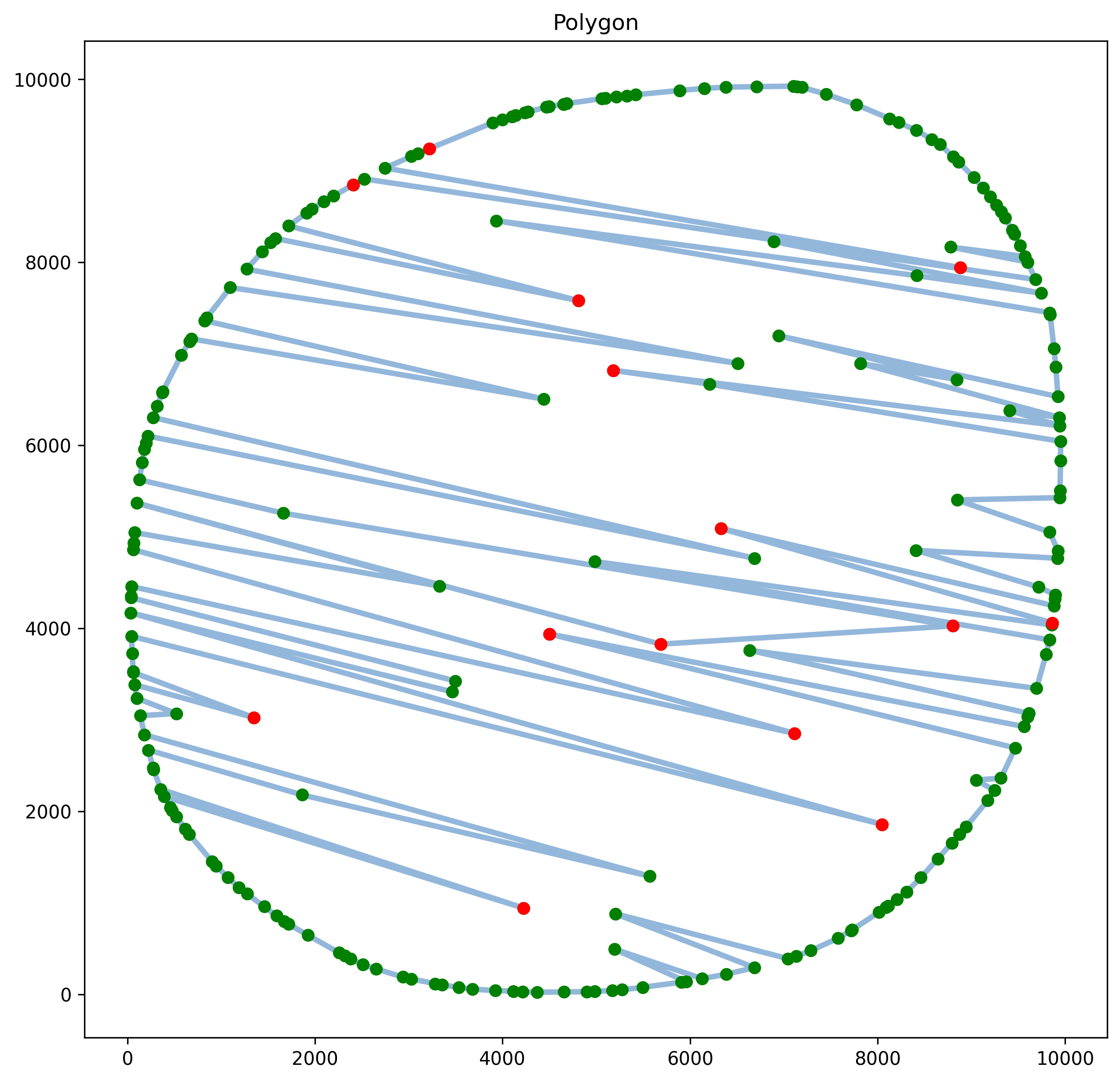
Figure 14: For polygon with $219$ vertices such that $r=34$ guard set in our new algorithm use $14$ guards and it runs in 670.436 s.

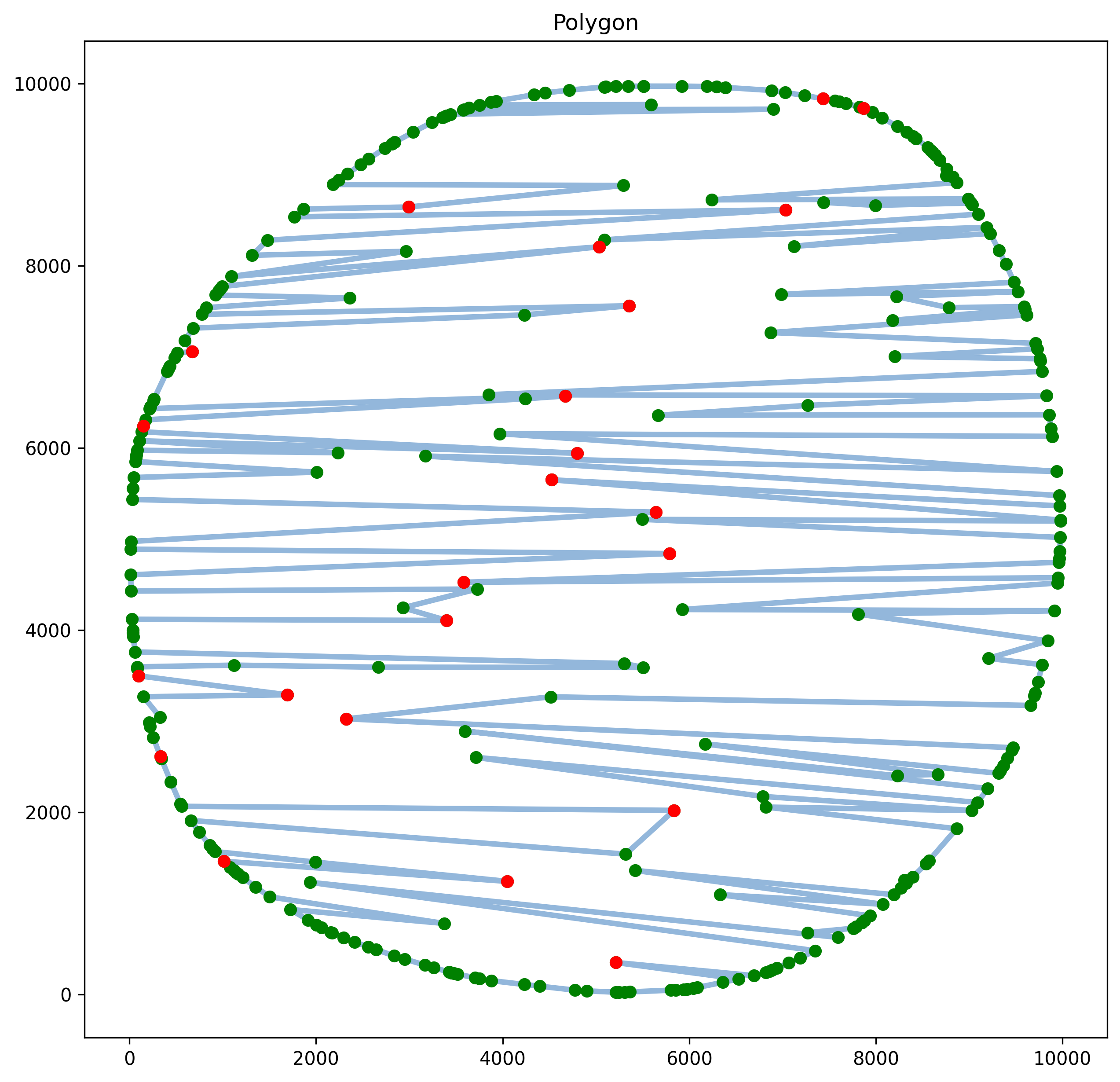
Figure 15: For polygon with $300$ vertices such that $r=65$ guard set in our new algorithm use $23$ guards and it runs in 520.861 s.

The outputs of test suggest that (see Figure 14 and Figure 15) even if $E$ reduces, the chosen guard set remains close to optimal and the algorithm assigns no more than twice the optimal number of guards.

4 Conclusion

In this paper we established that the Ghosh conjecture in 1986 was that through his approximation algorithm is O(log n) times optimal theoretically, it will perform much better in practice. All the experimental data that are provided in the entire paper shows that even for complex simple polygons, the chosen guard set by the algorithm is very close to optimal. Therefore, Ghosh’s algorithm performs like a constant approximation algorithm in practice.

Acknowledgments.

The work is inspired and guided by Prof Subir Kumar Ghosh.

References

- [1] Pritam Bhattacharya, Subir Kumar Ghosh, and Bodhayan Roy. Approximability of guarding weak visibility polygons. Discrete Applied Mathematics, 228:109–129, 2017.
- [2] Vasek Chvátal. A combinatorial theorem in plane geometry. Journal of Combinatorial Theory, Series B, 18(1):39–41, 1975.
- [3] Subir Kumar Ghosh. Visibility algorithms in the plane. Cambridge university press, 2007.
- [4] Subir Kumar. Ghosh. Approximation algorithms for art gallery problems in polygons. Discrete Applied Mathematics, 158(6), 2010.
- [5] Jeff Kahn, Maria Klawe, and Daniel Kleitman. Traditional galleries require fewer watchmen. SIAM Journal on Algebraic Discrete Methods, 4(2):194–206, 1983.
- [6] D Lee and Arthurk Lin. Computational complexity of art gallery problems. IEEE Transactions on Information Theory, 32(2):276–282, 1986.
- [7] Joseph O’Rourke. An alternate proof of the rectilinear art gallery theorem. Journal of Geometry, 21(1):118–130, 1983.