Minimax Flow over Acyclic Networks:
Distributed Algorithms and Microgrid Application

Abstract.  Given a flow network with variable suppliers and fixed consumers, the minimax flow problem consists in minimizing the maximum flow between nodes, subject to flow conservation and capacity constraints. We solve this problem over acyclic graphs in a distributed manner by showing that it can be recast as a consensus problem between the maximum downstream flows, which we define here for the first time. Additionally, we present a distributed algorithm to estimate these quantities. Finally, exploiting our theoretical results, we design an online distributed controller to prevent overcurrent in microgrids consisting of loads and droop-controlled inverters. Our results are validated numerically on the CIGRE benchmark microgrid.

Introduction

Problem description and motivation

Flow networks are dynamical systems where a commodity of interest is provided by supplier nodes, flows over the network edges, and reaches consumer nodes. Critical infrastructure networks such as power grids, water distribution networks, and traffic networks are modeled as flow networks, with the commodity of interest being electrical power, water, and vehicles, respectively [1, 2, 3]. A fundamental problem in these networks is to cater for consumers’ demands, while keeping the commodity flows over the network edges below their maximum capacities. Hence, a valuable optimization problem is to minimize the maximum flow over the network edges, thereby ensuring that no edge capacity is exceeded. Violation of capacity constraints is a safety-critical event, with a potential to cause disruptions or faults in real-world infrastructure networks. Typically, the resulting minimax flow problem is solved offline in a centralized fashion, so that the “right” flows can be assigned to the network edges. However, recent changes in infrastructure networks, due to the increase in demand, the integration of numerous smart devices and the need for higher energy efficiency, have shown the limitations of such centralized approaches.

In this paper, we propose a distributed solution to the minimax flow problem over acyclic networks consisting of suppliers and consumer nodes, where the former can adjust their supply rates to satisfy fixed consumption demands in the latter. In particular, by solving a distributed consensus problem, we propose a strategy for supplier generation that minimizes the maximum flow over all edges, subject to flow conservation and safety constraints. As a case study of relevance in applications, we apply our distributed approach to AC microgrids consisting of resistive loads and droop-controlled distributed energy units. We show that our algorithm is an effective solution to adjust the suppliers’ generation rates in order to prevent overcurrents on the network edges while fulfilling the demands of the consumers.

Literature on network optimization problems

One of the earliest formulations of minimax optimization problems on graphs is the minimax location problem [4], where the objective function is the distance between a facility node to be placed in the network and the other nodes in the graph. Later studies on this topic include [5, 6]. In [7, 8], the time-minimizing transportation problem was studied, where source nodes and sink nodes are two disjoint sets making up a bipartite graph, and the objective is to minimize the maximum transportation time among all utilized edges. In [9], the minimax transportation problem is introduced for cyclic graphs with one source node and one sink node, with the objective of minimizing the maximum flow in the network. Later, in [10], the problem is recast as a linear program and several solution algorithm are presented.

Surprisingly, to the best of our knowledge, relatively few distributed solutions of minimax problems on graphs have been presented in the existing literature (see [11] for a recent review of distributed network optimization algorithms). Examples of existing distributed approaches, although not applicable to minimax flow problems, include those presented in [12], where two networks are in competition to maximize and minimize an objective function, and [13], where agents are divided into two groups for computing two continuous decision variables in a minimax optimization. For the specific case of flow networks, a Newton-based distributed algorithm is presented in [14] for minimizing the sum of all flows, while an accelerated algorithm for a similar problem is described in [15]. Also, a distributed algorithm for minimizing the $p$-norm of flows was presented in [16], which approximates the minimax flow problem when $p$ becomes very large.

Literature on microgrid protection

Protection against faults (such as overcurrents) in microgrids can be ensured through three kinds of interventions: prevention (before the unwanted events), detection (during the events), and management (right after the events). In the literature, most studies focus on detection and management (see [17, 18, 19] and references therein). However, fault prevention is one area in which the use of intelligent control strategies could prove particularly fruitful, given the many challenges with fault detection and management algorithms currently available for microgrids [20, 21, 22].

An optimization problem to find the maximum permissible loading is solved in [20] through genetic algorithms, to prevent the occurrence of cascading failures. Overvoltages are prevented in [21] via a decentralized control scheme that curtails the active power output of the generators when necessary, while a control strategy is presented in [22] to prevent overloading of distributed generators during peak demand time, employing battery storage units that can intervene smoothly. Further distributed control strategies for microgrids include [23, 24, 25, 26, 27, 28] but are not specifically aimed at solving minimax problems. A minimax optimization problem for networks of microgrids is solved in a distributed fashion in [29], minimizing a function of the energy stored in the microgrids and the power flows between them, controlling the latter.

Contributions

The key contributions of this paper can be summarized as follows:

1. we establish a connection between solving the minimax flow problem over an acyclic graph and achieving consensus of the maximum downstream flows, that we define here for the first time;

2. we propose a distributed estimation strategy to evaluate the maximum downstream flows of a network of interest;

3. we exploit our theoretical results and an estimation strategy to obtain an online distributed controller to minimize the maximum power flow on the lines of a microgrid, by adjusting dynamically the power generated by the suppliers, thus preventing overcurrents in the grid.

When compared to the existing literature, our objectives and methodology are closer in flavor to those presented in [16], with the important differences that therein (i) consumers can absorb any amount of commodity and (ii) only an approximate solution of the minimax flow problem is obtained. All the other references we reviewed differ from our work in major aspects, such as the optimization problem (e.g., minisum rather than minimax, as in [15]) or the network structure (e.g., single source and single sink, with cyclic graphs, as in [30]).

Review of flow networks

Notation

We let $\max(\varnothing)=0$. Letting $\mathcal{Q}$ and $\mathcal{R}$ be sets, $\lvert\mathcal{Q}\rvert$ is the cardinality of $\mathcal{Q}$, and $\mathcal{Q}\rightrightarrows\mathcal{R}$ is an application from $\mathcal{Q}$ to all subsets of $\mathcal{R}$. Given a matrix $\mathbf{A}$, $\mathrm{ker}(\mathbf{A})$ is its null space (kernel), and $\mathbf{A}^{\dagger}$ is its Moore-Penrose (pseudo-)inverse [31].

Graph theory

Letting $\mathcal{G}=(\mathcal{V},\mathcal{E})$ be a graph, $\mathcal{V}$ and $\mathcal{E}$ are the set of vertices and the set of edges, respectively; $N\triangleq\left|\mathcal{V}\right|$ and $N_{\mathcal{E}}\triangleq\left|\mathcal{E}\right|$ being the numbers of vertices and edges. We denote an undirected edge connecting vertices $i$ and $j$ as $\{i,j\}$, and a directed edge from $i$ to $j$ as $(i,j)$. $\mathbf{A}$ and $\mathbf{L}$ are the adjacency and Laplacian matrices associated to $\mathcal{G}$. In an undirected graph, we let $\mathcal{Q}$ be the set of edges in $\mathcal{E}$, after they have been enumerated and oriented in an arbitrary way, and let $\mathbf{B}$ be the incidence matrix associated to the graph $(\mathcal{V},\mathcal{Q})$. In a (directed) graph, a (directed) path is an ordered sequence of vertices such that any pair of consecutive vertices is an edge in the graph. In a directed graph $(\mathcal{V},\vec{\mathcal{E}})$, the out-tree of vertex $i\in\mathcal{V}$ is the union of all directed paths starting from $i$; moreover, the out-neighborhood of a vertex $i$ is the set of all vertices $j$ such that a directed edge $(i,j)$ exists in $\vec{\mathcal{E}}$.

Flow networks

Consider a flow network associated to an undirected acyclic unweighted graph $\mathcal{G}=(\mathcal{V},\mathcal{E})$. We define $\mathcal{V}_{\mathrm{s}}\subset\mathcal{V}$ as the set of supplier vertices and $\mathcal{V}_{\mathrm{c}}\subset\mathcal{V}$ as the set of consumer vertices, with $\{\mathcal{V}_{\mathrm{s}},\mathcal{V}_{\mathrm{c}}\}$ being a partition of $\mathcal{V}$. Additionally, we let $N_{\mathrm{s}}\triangleq\left|\mathcal{V}_{\mathrm{s}}\right|\geq 2$ and $N_{\mathrm{c}}\triangleq\left|\mathcal{V}_{\mathrm{c}}\right|\geq 1$ be the number of supplier and consumer vertices, respectively.

Commodity

We let $m_{i}\in\mathbb{R}$ be the amount of commodity supplied ($m_{i}>0$) or consumed ($m_{i}\leq 0$) at vertex $i$, and define $\mathbf{m}\triangleq[m_{i}]_{i\in\mathcal{V}}\in\mathbb{R}^{N}$ and $\mathbf{m}_{\mathrm{s}}\triangleq[m_{i}]_{i\in\mathcal{V}_{\mathrm{s}}}\in\mathbb{R}^{N_{\mathrm{s}}}$. We assume that the amounts of consumed commodity ($m_{i},i\in\mathcal{V}_{\mathrm{c}}$) are given, whereas the amounts of supplied commodity ($m_{i},i\in\mathcal{V}_{\mathrm{s}}$) can be controlled, provided that $\mathbf{m}_{\mathrm{min}}\leq\mathbf{m}_{\mathrm{s}}\leq\mathbf{m}_{\mathrm{max}}$, where $\mathbf{m}_{\mathrm{min}},\mathbf{m}_{\mathrm{max}}\in\mathbb{R}_{>0}^{N_{\mathrm{s}}}$ are vectors of positive real numbers.

Flows

For all $\{i,j\}\in\mathcal{E}$, we let $f_{ij}\in\mathbb{R}$ denote the flow of commodity from $i$ to $j$; $f_{ij}>0$ if commodity flows from $i$ to $j$ and vice-versa, and $f_{ji}=-f_{ij}$. We also define $\mathbf{f}=[f_{ij}]_{(i,j)\in\mathcal{Q}}\in\mathbb{R}^{N_{\mathcal{E}}}$. The flows satisfy the balancing equations

$${}\sum_{j:\{i,j\}\in\mathcal{E}}f_{ij}=m_{i},\quad\forall i\in\mathcal{V},$$ (2.1)

which can be written in a more compact form as

$$\mathbf{B}\mathbf{f}=\mathbf{m}.$$ (2.2)

Finally, we let $\bar{f}_{ij}\in\mathbb{R}_{>0}$ be the capacity (i.e., maximum flow allowed) of edge $\{i,j\}$, and define $\bar{\mathbf{f}}=[\bar{f}_{ij}]_{(i,j)\in\mathcal{Q}}\in\mathbb{R}_{>0}^{N_{\mathcal{E}}}$.

Next, we present a result characterizing flows over acyclic networks. For completeness’ sake, we include a short proof.

[Flows [32]] In an acyclic unweighted undirected flow network with incidence matrix $\mathbf{B}$, Laplacian matrix $\mathbf{L}$, and commodity vector $\mathbf{m}$, the flows $\mathbf{f}$ are uniquely determined by commodity conservation (2.2) and are given by

$$\mathbf{f}=\mathbf{B}^{\mathsf{T}}\mathbf{L}^{\dagger}\mathbf{m}.$$ (2.3)

Proof.

From [28], we have $\mathbf{L}^{\dagger}\mathbf{L}=\mathbf{I}-\frac{1}{N}\mathbf{1}\mathbf{1}^{\mathsf{T}}$, and, as the graph is unweighted, $\mathbf{L}=\mathbf{B}\mathbf{B}^{\mathsf{T}}$ [33, Chapter 9]. Then, consider the following expression: $\mathbf{B}^{\mathsf{T}}\mathbf{L}^{\dagger}\mathbf{B}\mathbf{B}^{\mathsf{T}}=\mathbf{B}^{\mathsf{T}}\mathbf{L}^{\dagger}\mathbf{L}=\mathbf{B}^{\mathsf{T}}(\mathbf{I}-\frac{1}{N}\mathbf{1}\mathbf{1}^{\mathsf{T}})=\mathbf{B}^{\mathsf{T}}$. As the graph is acyclic, $\mathrm{ker}(\mathbf{B})=\varnothing$ [33], and thus $\mathbf{B}^{\mathsf{T}}\mathbf{L}^{\dagger}\mathbf{B}=\mathbf{I}.$ Therefore, premultiplying (2.2) by $\mathbf{B}^{\mathsf{T}}\mathbf{L}^{\dagger}$, we get the thesis. ∎

Problem formulation

Minimax flow problem

We start by defining the flow safety margin of a network.

[Flow safety margin] Given a flow network over $\mathcal{G}=(\mathcal{V},\mathcal{E})$ with supplied commodity $\mathbf{m}_{\mathrm{s}}$, flows $f_{ij}$ and capacities $\bar{f}_{ij}$, the flow safety margin $J_{\mathcal{E}_{\mathrm{r}}}:\mathbb{R}^{N_{\mathrm{s}}}\rightarrow\mathbb{R}_{\geq 0}$, with respect to a given edge set $\mathcal{E}_{\mathrm{r}}\subseteq\mathcal{E}$ is

$$J_{\mathcal{E}_{\mathrm{r}}}(\mathbf{m}_{\mathrm{s}})\triangleq\max_{\{i,j\}\in\mathcal{E}_{\mathrm{r}}}\frac{\left|f_{ij}\right|}{\bar{f}_{ij}}.$$ (3.1)

$J_{\mathcal{E}_{\mathrm{r}}}\geq 1$ corresponds to a fault condition we wish to avoid. We now state the main problem under study in this paper.

Problem (Minimax flow problem).

For a flow network over an acyclic graph, the minimax flow problem is

$$\min_{\mathbf{m}_{\mathrm{s}}} \ J_{\mathcal{E}_{\mathrm{r}}}(\mathbf{m}_{\mathrm{s}}),$$ (3.2)

$$\mathrm{s.t.\ } \begin{dcases}\mathbf{B}\mathbf{f}=\mathbf{m},\\ \textstyle\sum_{i\in\mathcal{V}}m_{i}=0,\\ \left|\mathbf{f}\right|<\bar{\mathbf{f}},\\ \mathbf{m}_{\mathrm{min}}\leq\mathbf{m}_{\mathrm{s}}\leq\mathbf{m}_{\mathrm{max}}.\end{dcases}$$

Following the steps in [10] and exploiting (2.3), it is straightforward to verify that the minimax flow problem is a linear program and can be solved using standard centralized iterative approaches. However, such an approach has two major drawbacks: (i) it requires receiving data from all edges and transmitting data to all the suppliers, which can be impractical; (ii) if $m_{i},i\in\mathcal{V}_{\mathrm{c}}$ are time-varying, the optimization problem needs to be solved repeatedly and if the re-computation is not fast enough, faults may occur from applying control inputs that are not up to date, as we will show in Section 6.3.

As explained below, it might occur that the flow can be controlled only on a subset of the edges, say $\mathcal{E}_{\mathrm{cf}}$; therefore, in the rest of this paper, when considering Problem 3.1 and the flow safety margin function $J_{\mathcal{E}_{\mathrm{r}}}$ in Definition 3.1, we take ${\mathcal{E}_{\mathrm{r}}}=\mathcal{E}_{\mathrm{cf}}$, and omit the subscript of $J_{\mathcal{E}_{\mathrm{cf}}}$ (writing $J$), for the sake of brevity. Next, we give a formal definition and characterization of the subset of edges with controllable flows $\mathcal{E}_{\mathrm{cf}}$.

Edges with controllable flows

Given an undirected graph $\mathcal{G}=(\mathcal{V},\mathcal{E})$ associated to a flow network, a set of directed edges $\vec{\mathcal{E}}$ is obtained by orienting the edges in $\mathcal{E}$ according to the direction of the flows on them. Namely, for each $\{i,j\}\in\mathcal{E}$, $\vec{\mathcal{E}}$ contains either edge $(i,j)$ if $f_{ij}>0$, or $(j,i)$ if $f_{ij}<0$, or no edge if $f_{ij}=0$. We also define the extended set of directed edges $\vec{\mathcal{E}}^{+}$ as the set that, for each $\{i,j\}\in\mathcal{E}$, contains both $(i,j)$ and $(j,i)$ (independently of the value of $f_{ij}$). These sets are portrayed in Figure 1.

[figure]style=plain,subcapbesideposition=top

[]

[]

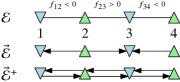
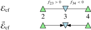
Figure 1: (a), (b): The various edges sets used in the paper, for a simple flow network. Upward green triangles represent suppliers, while downward blue triangles denote consumers.

[Half-cluster] For an acyclic undirected graph $\mathcal{G}=(\mathcal{V},\mathcal{E})$, the half-cluster is a function $\mathcal{H}:\vec{\mathcal{E}}^{+}\rightrightarrows\mathcal{V}$. In particular, $\mathcal{H}[(i,j)]=\mathcal{H}_{ij}$ is the set of vertices in the connected component of $\mathcal{G}\setminus\{i\}$ that contains $j$ (Figure 2).

[Supplier indicator function] For an acyclic flow network, the supplier indicator function $\beta:\vec{\mathcal{E}}^{+}\rightarrow\{0,1\}$ is defined as

$$\beta[(i,j)]=\beta_{ij}\triangleq\begin{dcases}1,&\text{if}\ \mathcal{V}_{\mathrm{s}}\cap\mathcal{H}_{ij}\neq\varnothing,\\ 0,&\text{otherwise}.\end{dcases}$$ (3.3)

In simple terms, $\beta_{ij}$ is $1$ if a supplier can be be found in $\mathcal{H}_{ij}$; moreover, notice that in general $\beta_{ij}$ is unrelated to $\beta_{ji}$. A graphical example is given in Figure 2.

[figure]style=plain,subcapbesideposition=top

[]

[]

[]

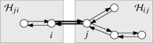
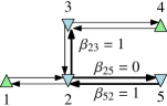
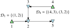
Figure 2: (a): Half-clusters $\mathcal{H}$ of edges $(j,i)$ (left) and $(i,j)$ (right) in an example graph $(\mathcal{V},\vec{\mathcal{E}}^{+})$. (b): Supplier indicator function $\beta$ for several edges, in an example graph $(\mathcal{V},\vec{\mathcal{E}}^{+})$; upward green triangles represent suppliers; downward blue triangles denote consumers. (c): Some downstreams $\mathcal{D}_{i}$ in an example graph $(\mathcal{V},\vec{\mathcal{E}})$.

As stated in the next Lemma, some flows $f_{ij}$ do not depend on the amount of commodity generated by supplier vertices, and thus we will not consider them in the optimization problem. We define the set of edges with controllable flows as

$$\mathcal{E}_{\mathrm{cf}}\triangleq\{\{i,j\}\in\mathcal{E}\mid\beta_{ij}=1\wedge\beta_{ji}=1\}.$$ (3.4)

[Non-controllable flows] In an acyclic flow network, the flows $f_{ij}$ for $\{i,j\}\in\mathcal{E}\setminus\mathcal{E}_{\mathrm{cf}}$ are independent of the supplied commodity $m_{k}$, $\forall k\in\mathcal{V}_{\mathrm{s}}$.

Proof.

Consider an edge $\{i,j\}\in\mathcal{E}\setminus\mathcal{E}_{\mathrm{cf}}$; by (3.4), it holds that $\beta_{ij}=0\ \vee\ \beta_{ji}=0$. Without loss of generality, assume that $\beta_{ij}=0$, which means that $\mathcal{H}_{ij}$ contains no suppliers. Then, using (2.1) for all vertices in $\mathcal{H}_{ij}$, we have that all edges reaching a vertex in $\mathcal{H}_{ij}$ (including $\{i,j\}$) have their flows only determined by ${\{m_{q}\}}_{q\in\mathcal{H}_{ij}}$. As $\mathcal{H}_{ij}\cap\mathcal{V}_{\mathrm{s}}=\varnothing$, we conclude that these flows do not depend on any $m_{k}$, for $k\in\mathcal{V}_{\mathrm{s}}$. ∎

We define $\mathcal{V}_{\mathrm{cf}}$ as the set of vertices that are reached by at least an edge in $\mathcal{E}_{\mathrm{cf}}$, and the graph $\mathcal{G}_{\mathrm{cf}}=(\mathcal{V}_{\mathrm{cf}},\mathcal{E}_{\mathrm{cf}})$. It is immediate to verify that this graph (i) cuts out from $\mathcal{G}$ the branches that contain only consumers, (ii) is connected, and (iii) all of its leaf vertices are suppliers. Finally, we let $\vec{\mathcal{E}}_{\mathrm{cf}}$ be the set of directed edges obtained by orienting the edges in $\mathcal{E}_{\mathrm{cf}}$ according to the flows, similarly to what we did to obtain $\vec{\mathcal{E}}$ from $\mathcal{E}$. Examples of $\mathcal{E}_{\mathrm{cf}}$ and $\vec{\mathcal{E}}_{\mathrm{cf}}$ are depicted in Figure 1.

Consensus reformulation of the minimax flow problem

Next, we introduce the notions of maximum downstream flows and consumer clusters which will then be used to reformulate the minimax flow optimization problem (Problem 3.1) as a consensus problem.

[maximum downstream flows and edges] Consider a flow network associated to an acyclic graph $\mathcal{G}=(\mathcal{V},\mathcal{E})$. Then,

1. for $i\in\mathcal{V}$, the downstream of vertex $i$, denoted by $\mathcal{D}_{i}\subseteq\vec{\mathcal{E}}_{\mathrm{cf}}$, is the out-tree of vertex $i$ in $(\mathcal{V}_{\mathrm{cf}},\vec{\mathcal{E}}_{\mathrm{cf}})$ (Figure 2);

2. the maximum downstream flow $\phi:\mathcal{V}\rightarrow\mathbb{R}_{\geq 0}$ is given by

   $$\phi(i)=\phi_{i}\triangleq\max_{(j,k)\in\mathcal{D}_{i}}\frac{f_{jk}}{\bar{f}_{jk}}\geq 0.$$ (4.1)

3. for $i\in\mathcal{V}$, the maximum downstream edge (MDE) of vertex $i$ is $\arg\max_{(j,k)\in\mathcal{D}_{i}}{f_{jk}/\bar{f}_{jk}}\in\vec{\mathcal{E}}_{\mathrm{cf}}$ (Figure 3).

If $i\in\mathcal{V}_{\mathrm{s}}$, we abbreviate “maximum downstream edge of a supplier vertex” as MDES. We denote by $\mathcal{M}_{\mathrm{s}}\subseteq\vec{\mathcal{E}}_{\mathrm{cf}}$ the set of all MDESs, and by $\mathcal{M}_{\mathrm{s}\rightarrow\mathrm{c}}\subseteq\mathcal{M}_{\mathrm{s}}$ the set of MDESs that have consumers as terminal vertices (see again Figure 3).

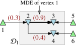
Figure 3: Representation of a maximum downstream edge (MDE). Upward green triangles represent suppliers, while downward blue triangles denote consumers; in red and in parentheses we drew $f_{ij}/\bar{f}_{ij}$. Edge $(2,3)$ is the MDE of vertex $1$. Moreover, as vertex $1$ is a supplier, $(2,3)$ is a maximum downstream edge of a supplier vertex (MDES; i.e., $(2,3)\in\mathcal{M}_{\mathrm{s}}$), and, as vertex $3$ is a consumer, then also $(2,3)\in\mathcal{M}_{\mathrm{s}\rightarrow\mathrm{c}}$.

We give next two instrumental results in Lemmas 4 and 4.

In an acyclic flow network, $\vec{\mathcal{E}}_{\mathrm{cf}}=\bigcup_{i\in\mathcal{V}_{\mathrm{s}}}\mathcal{D}_{i}$.

Proof.

We obtain a proof by contradiction, showing that if the thesis did not hold, that would cause some consumer vertices not to receive as much commodity as they demand (which would contradict (2.1)). In particular, contrary to the thesis, assume that there exists $(j,k)\in\vec{\mathcal{E}}_{\mathrm{cf}}$ such that

$$(j,k)\notin\bigcup_{i\in\mathcal{V}_{\mathrm{s}}}\mathcal{D}_{i}.$$ (4.2)

Define $\mathcal{S}$ as the set of vertices that have $(j,k)$ in their out-tree (see Figure 4). By Definition 4.i, (4.2) implies that all nodes in $\mathcal{S}$ are not suppliers (and thus are consumers), because the right-hand side in (4.2) is computed considering $i\in\mathcal{V}_{\mathrm{s}}$. Moreover, let $\mathcal{E}_{\mathcal{S}}\triangleq\{(p,q)\in\vec{\mathcal{E}}_{\mathrm{cf}}\mid p\notin\mathcal{S},q\in\mathcal{S}\}$ (i.e., edges “on the boundary” of $\mathcal{S}$ that terminate in $\mathcal{S}$). It is immediate to see that

$$\mathcal{E}_{\mathcal{S}}=\varnothing;$$ (4.3)

indeed, if there existed an edge $(p,q)\in\mathcal{E}_{\mathcal{S}}$, then $(j,k)$ would belong to the out-tree of $p$, which by definition of $\mathcal{S}$ would imply $p\in\mathcal{S}$, but this is impossible by definition of $\mathcal{E}_{\mathcal{S}}$.

However, exploiting (2.1) for $i\in\mathcal{V}_{\mathrm{c}}$, we have that $\sum_{(j,k)\in\mathcal{E}_{\mathcal{S}}}f_{jk}=-\sum_{q\in\mathcal{S}}m_{q}>0$, which requires that $\mathcal{E}_{\mathcal{S}}\neq\varnothing$, but this is in contradiction with (4.3). Therefore, an edge $(j,k)$ that satisfies (4.2) cannot exist, and the thesis is proved. ∎

Figure 4: Graph topology described in the proof of Lemma 4. Downward triangles represents consumers, while circles can either be suppliers or consumers.

[Consumer cluster] In an acyclic flow network, a consumer cluster $\mathcal{C}\subset\mathcal{V}_{\mathrm{cf}}$ is a set of vertices having the following properties (see Figure 5):

1. all vertices in $\mathcal{C}$ are consumers ($\mathcal{C}\subseteq\mathcal{V}_{\mathrm{c}}\cap\mathcal{V}_{\mathrm{cf}}$), and $\mathcal{C}$ is a connected component in $\mathcal{G}_{\mathrm{cf}}=(\mathcal{V}_{\mathrm{cf}},\mathcal{E}_{\mathrm{cf}})$;

2. there are no MDESs between the vertices in $\mathcal{C}$, i.e., $\mathcal{M}_{\mathrm{s}}\cap(\mathcal{C}\times\mathcal{C})=\varnothing$;

3. any edge $(i,j)$ or $(j,i)$, where $i$ is a consumer not belonging to $\mathcal{C}$ and $j$ is a vertex in $\mathcal{C}$, must be an MDES;

4. there exists at least an MDES that terminates in $\mathcal{C}$, i.e., $\exists(i,j)\in\mathcal{M}_{\mathrm{s}\rightarrow\mathrm{c}}:j\in\mathcal{C}$.

Given a consumer cluster $\mathcal{C}$, we denote by $\mathcal{E}_{\mathcal{C}}\subseteq\vec{\mathcal{E}}_{\mathrm{cf}}$ the set of directed edges that are on the boundary of $\mathcal{C}$, i.e., $\mathcal{E}_{\mathcal{C}}\triangleq\{(i,j)\in\vec{\mathcal{E}}_{\mathrm{cf}}\mid(i\in\mathcal{C},j\not\in\mathcal{C})\vee(i\not\in\mathcal{C},j\in\mathcal{C})\}$. Moreover, we denote by $\hat{\mathcal{C}}$ the set of all consumer clusters and note the following facts. Firstly, $\hat{\mathcal{C}}$ is finite because the number of vertices in $\mathcal{V}_{\mathrm{cf}}$ is finite. Secondly, any two different consumer clusters $\mathcal{C}_{1},\mathcal{C}_{2}\in\hat{\mathcal{C}}$ must be disjoint, because of properties ii-iii in Definition 4. Thirdly, by Definition 4, any edge in $\mathcal{M}_{\mathrm{s}\rightarrow\mathrm{c}}$ terminates in a consumer cluster.

[Critical consumer cluster] In an acyclic flow network, A critical consumer cluster $\mathcal{C}^{*}$ is a consumer cluster such that all $(i,j)\in\mathcal{E}_{\mathcal{C}^{*}}$ terminate in $\mathcal{C}^{*}$ and are MDESs (see Figure 5), i.e.,

$$\forall(i,j)\in\mathcal{E}_{\mathcal{C}^{*}},\quad(i,j)\in\mathcal{M}_{\mathrm{s}\rightarrow\mathrm{c}}\wedge j\in\mathcal{C}^{*}.$$ (4.4)

[Existence of critical consumer cluster] In an acyclic flow network, if $\phi_{i}>0$ for all $i\in\mathcal{V}_{\mathrm{s}}$, then there exists a critical consumer cluster.

Proof.

First, note that the hypothesis $\phi_{i}>0,\forall i\in\mathcal{V}_{\mathrm{s}}$ implies that all suppliers have a MDE (that is a MDES; see Definition 4.iii). This, in conjunction with the facts that the network has an acyclic structure and that the number of vertices is finite, implies that there exists at least a MDES terminating in a consumer, i.e., $\mathcal{M}_{\mathrm{s}\rightarrow\mathrm{c}}\neq\varnothing$, which yields $\hat{\mathcal{C}}\neq\varnothing$.

Next, we prove the thesis by contradiction. Negating the existence of a critical consumer cluster, we have, from (4.4),

$$\forall\mathcal{C}\in\hat{\mathcal{C}},\exists(i,j)\in\mathcal{E}_{\mathcal{C}}:\quad(i,j)\notin\mathcal{M}_{\mathrm{s}\rightarrow\mathrm{c}}\vee j\notin\mathcal{C}.$$ (4.5)

Let us consider some $\mathcal{C}_{1}\in\hat{\mathcal{C}}$ and assume without loss of generality that the edge $(i,j)$ referenced in (4.5) is such that $i\notin\mathcal{C}_{1}$ and $j\in\mathcal{C}_{1}$ (i.e., $(i,j)$ ends in $\mathcal{C}_{1}$; see Figure 5). In this case, it remains to be proved that assuming $(i,j)\notin\mathcal{M}_{\mathrm{s}\rightarrow\mathrm{c}}$ leads to a contradiction. Indeed, in this case either $i$ is a supplier or it is a consumer. In this latter case, by Definition 4 (see in particular point iii), $i$ must belong to $\mathcal{C}_{1}$, which is against the hypothesis. If $i$ is a supplier instead, then it must have some MDES, say $a\in\mathcal{M}_{\mathrm{s}}$, that cannot be $(i,j)$ or belong to $\mathcal{C}_{1}$ by Definition 4 (point ii). Then, either $a$ ends in a consumer or in a supplier. If it ends in a consumer, then $a$ must end in some consumer cluster $\mathcal{C}_{2}$ different from $\mathcal{C}_{1}$, given the property that the graph is acyclic by hypothesis. On the other hand, if $a$ ends in a supplier, then that supplier must have its own MDES and the argument can be repeated until an MDES ending in a consumer is found; hence, this MDES ends in a consumer cluster, which is different from any other defined earlier on in the procedure (because the graph $\mathcal{G}$ is acyclic). As this argument can be repeated ad infinitum, we get a contradiction (because $\hat{\mathcal{C}}$ must be finite) and the theorem remains proved.

A similar argument could be used to reach a contradiction if the edge $(i,j)$ is assumed to be such that $i\in\mathcal{C}_{1}$ and $j\notin\mathcal{C}_{1}$ (i.e., $(i,j)$ does not end in $\mathcal{C}_{1}$). Therefore, we conclude that (4.5) does not hold, which corresponds to the thesis. ∎

[]

[]

[]

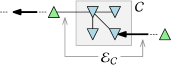
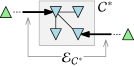
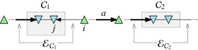
Figure 5: (a): A consumer cluster $\mathcal{C}$ (see Definition 4); upward green triangles represent suppliers, while downward blue triangles denote consumers; heavier arrows denote MDESs; dots represents connected components of vertices. (b): A critical consumer cluster $\mathcal{C}^{*}$ (see Lemma 4). (c): Situation described in the proof of Lemma 4.

We are now ready to present our main result.

[Consensus achieves optimization] In an acyclic flow network, if $\phi_{i}=\phi^{*}$ for all $i\in\mathcal{V}_{\mathrm{s}}$ and for some $\phi^{*}\in\mathbb{R}_{\geq 0}$, then the cost function $J$ (see Definition 3.1) is minimized with respect to $\mathbf{m}_{\mathrm{s}}$.

Proof.

From (3.1), exploiting Lemma 4, and using (4.1), we have

$$J=\max_{\{i,j\}\in\mathcal{E}_{\mathrm{cf}}}\frac{\left|f_{ij}\right|}{\bar{f}_{ij}}=\max_{(i,j)\in\vec{\mathcal{E}}_{\mathrm{cf}}}\frac{f_{ij}}{\bar{f}_{ij}}=\max_{(i,j)\in{\bigcup_{i\in\mathcal{V}_{\mathrm{s}}}\mathcal{D}_{i}}}\frac{f_{ij}}{\bar{f}_{ij}}=\max_{i\in\mathcal{V}_{\mathrm{s}}}\phi_{i}.$$ (4.6)

From (4.6), it is obvious that, if $\phi^{*}=0$, then $J=0$, which clearly corresponds to the lowest possible value of $J$.

We consider next the case that $\phi^{*}>0$. For the sake of brevity, let $x_{ij}\triangleq f_{ij}/\bar{f}_{ij}$. From Lemma 4, there exists a critical consumer cluster $\mathcal{C}^{*}$, and using (4.6) and the fact that $\mathcal{E}_{\mathcal{C}^{*}}\subseteq\vec{\mathcal{E}}_{\mathrm{cf}}$ we have

$$J\geq\tilde{J}\triangleq\max_{(i,j)\in\mathcal{E}_{\mathcal{C}^{*}}}x_{ij}.$$ (4.7)

Then, from (2.1), it is straightforward to compute that

$$\sum_{(i,j)\in\mathcal{E}_{\mathcal{C}^{*}}}f_{ij}=-\sum_{k\in{\mathcal{C}^{*}}}m_{k},$$

which, letting $m_{\mathcal{C}^{*}}\triangleq-\sum_{k\in{\mathcal{C}^{*}}}m_{k}>0$, can be rewritten as $\sum_{(i,j)\in\mathcal{E}_{\mathcal{C}^{*}}}x_{ij}\bar{f}_{ij}=m_{\mathcal{C}^{*}}$. Therefore, considering the problem

$$\min_{x_{ij}\in\mathbb{R}_{\geq 0},(i,j)\in\mathcal{E}_{\mathcal{C}^{*}}} \tilde{J},$$

$$\mathrm{s.t.\ } \sum_{(i,j)\in\mathcal{E}_{\mathcal{C}^{*}}}x_{ij}\bar{f}_{ij}=m_{\mathcal{C}^{*}},$$

and recalling (4.7), it is clear that the minimum value of $\tilde{J}$ is achieved when all $x_{ij}$s are equal. At this point, by hypothesis, $x_{ij}=\phi^{*},\forall(i,j)\in\mathcal{E}_{\mathcal{C}^{*}}$, and thus $\tilde{J}=\phi^{*}$ is minimal. From (4.6) and the hypothesis, it also holds that $J=\phi^{*}$; therefore, from (4.7), $J$ is also minimized. ∎

Note that Theorem 5 offers only a sufficient condition for the solution of Problem 3.1.

Distributed estimation of maximum downstream flows

In this section, we study how the maximum downstream flows $\phi_{i}$ can be estimated by each node using a recursive process that only requires local information. Then, in Section 6, we embed such estimation process in a heuristic distributed control approach to achieve consensus of the maximum downstream flows, and hence solve Problem 3.1 via Theorem 5, for the case of electric microgrids.

Let us denote by $\mathcal{V}_{i}^{\mathrm{out}}$ the out-neighborhood of vertex $i$ in the graph $(\mathcal{V},\vec{\mathcal{E}})$.

[Reformulation of maximum downstream flows] In an acyclic flow network, the maximum downstream flow $\phi_{i}$ (see Definition 4.ii) can be found by computing

$$\phi_{i}=\max_{j\in\mathcal{V}^{\mathrm{out}}_{i}}\left\{\beta_{ij}\frac{f_{ij}}{\bar{f}_{ij}},\ \phi_{j}\right\}.$$ (5.1)

Proof.

Figure 6: Grouping of vertices in accordance to their values of $l_{\mathrm{p}}$, defined in the proof of Lemma 5, for an example graph $(\mathcal{V},\vec{\mathcal{E}})$.

For the sake of simplicity and without loss of generality, assume that $\bar{f}_{ij}=1$ and $\beta_{ij}=1$ for all $(i,j)\in\vec{\mathcal{E}}^{+}$. In the directed acyclic graph $(\mathcal{V},\vec{\mathcal{E}})$, let us denote by $l_{\mathrm{p}}(i)$ the maximum length of all directed paths starting from vertex $i$; then $\mathcal{V}_{0},\mathcal{V}_{1},\mathcal{V}_{2},\dots$ are the sets of vertices that have $l_{\mathrm{p}}=0,l_{\mathrm{p}}=1,l_{\mathrm{p}}=2,\dots$, respectively (see Figure 6). We show the thesis, i.e., that (5.1) is equivalent to (4.1), for the subsets $\mathcal{V}_{0},\mathcal{V}_{1},\mathcal{V}_{2},\dots$ one at a time.

• $k\in\mathcal{V}_{0}$.  As $\mathcal{D}_{k}=\mathcal{V}^{\mathrm{out}}_{k}=\varnothing$, both (4.1) and (5.1) yield

  $$\phi_{k}=0,\quad k\in\mathcal{V}_{0}.$$ (5.2)

• $j\in\mathcal{V}_{1}$.  We have $\mathcal{D}_{j}=\{(j,k)\mid k\in\mathcal{V}^{\mathrm{out}}_{j}\}$. This, together with (5.2), means that both (4.1) and (5.1) give

  $$\phi_{j}=\max\left\{f_{jk}\right\}_{k\in\mathcal{V}^{\mathrm{out}}_{j}},\quad j\in\mathcal{V}_{1}.$$ (5.3)

• $i\in\mathcal{V}_{2}$.  Now, $\mathcal{D}_{i}=\{(i,j)\mid j\in\mathcal{V}^{\mathrm{out}}_{i}\}\cup\{(j,k)\mid j\in\mathcal{V}^{\mathrm{out}}_{i},k\in\mathcal{V}^{\mathrm{out}}_{j}\}$, From (4.1), we have

  $$\phi_{i}=\mathrm{max}\left\{{\left\{f_{ij}\right\}}_{j\in\mathcal{V}^{\mathrm{out}}_{i}},{\left\{f_{jk}\right\}}_{j\in\mathcal{V}^{\mathrm{out}}_{i},k\in\mathcal{V}^{\mathrm{out}}_{j}}\right\},\quad i\in\mathcal{V}_{2}.$$ (5.4)

  Then, using (5.3), (5.4) can be rewritten as

  $$\phi_{i}=\mathrm{max}\left\{{\left\{f_{ij}\right\}}_{j\in\mathcal{V}^{\mathrm{out}}_{i}},{\left\{\phi_{j}\right\}}_{j\in\mathcal{V}^{\mathrm{out}}_{i}}\right\},\quad i\in\mathcal{V}_{2},$$

  which corresponds to (5.1).

• $h\in\{\mathcal{V}_{3},\dots,\mathcal{V}_{N-1}\}$.  The reasoning presented at the above point can be easily repeated to show that (5.1) is equivalent to (4.1) for all remaining vertices.

∎

In practice, the calculation in (5.1) can be implemented through an arbitrarily fast dynamical estimation system, as stated in the next proposition.

[Distributed estimation of maximum downstream flows] In an acyclic flow network, we let $\hat{\phi}:\mathcal{V}\times\mathbb{R}_{\geq 0}\rightarrow\mathbb{R}$—denoting $\hat{\phi}(i,t)$ by $\hat{\phi}_{i}(t)$—be the solution to

$$\dot{\hat{\phi}}_{i}(t)=-k_{\phi}\left(\hat{\phi}_{i}(t)-\max_{j\in\mathcal{V}^{\mathrm{out}}_{i}}\left\{\beta_{ij}\frac{f_{ij}}{\bar{f}_{ij}},\ \hat{\phi}_{j}(t)\right\}\right),\ \hat{\phi}_{i}(0)=0,$$ (5.5)

$\forall i\in\mathcal{V}$. Assume the $f_{ij}$s are constant, or $k_{\phi}\in\mathbb{R}_{>0}$ is large enough so that the $f_{ij}$s can be considered constant with respect to the dynamics of the $\hat{\phi}_{i}$s. Then, $\hat{\phi}_{i}$ converges to $\phi_{i}$, $\forall i\in\mathcal{V}$.

Proof.

As in the Proof of Lemma 5, for simplicity and without loss of generality, assume that $\bar{f}_{ij}=1$ and $\beta_{ij}=1$ for all $(i,j)\in\vec{\mathcal{E}}^{+}$; moreover, consider again the sets $\mathcal{V}_{0},\mathcal{V}_{1},\mathcal{V}_{2},\dots$ defined in that Proof and depicted in Figure 6.

• $k\in\mathcal{V}_{0}$.  From (5.5), we have

  $$\dot{\hat{\phi}}_{k}(t)=-k_{\phi}\hat{\phi}_{k}(t),\quad\hat{\phi}_{k}(0)=0,\quad k\in\mathcal{V}_{0}.$$

  Thus, for $k\in\mathcal{V}_{0}$, $\forall t$, $\hat{\phi}_{k}(t)=0=\phi_{k}$ (see (5.1)).

• $j\in\mathcal{V}_{1}$.  From (5.5) and what we stated at the previous point, we have

  $$\dot{\hat{\phi}}_{j}(t)=-k_{\phi}\left(\hat{\phi}_{j}(t)-\max_{k\in\mathcal{V}^{\mathrm{out}}_{j}}\left\{f_{jk},0\right\}\right),\quad j\in\mathcal{V}_{1}.$$ (5.6)

  Recall that all $f_{jk}$ can be considered constant by hypothesis. Therefore, $\forall j\in\mathcal{V}_{1}$, $\hat{\phi}_{j}$ converges exponentially fast to $\phi_{j}$, as given in (5.1).

• $i\in\mathcal{V}_{2}$.  From (5.5), we get

  $$\dot{\hat{\phi}}_{i}(t)=-k_{\phi}\left(\hat{\phi}_{i}(t)-\max_{j\in\mathcal{V}^{\mathrm{out}}_{i}}\left\{f_{ij},\hat{\phi}_{j}(t)\right\}\right),\quad i\in\mathcal{V}_{2}.$$ (5.7)

  After a short time, all $\hat{\phi}_{j}$, $j\in\mathcal{V}_{1}$, can be considered at steady state. Thus, clearly $\hat{\phi}_{i}$ converges to $\phi_{i}$ (as given in (5.1)), for all $i\in\mathcal{V}_{2}$.

• $h\in\{\mathcal{V}_{2},\dots,\mathcal{V}_{N-1}\}$.   The above steps can be repeated to show the thesis for the remaining nodes.

∎

To compute the generator indicator function $\beta$ appearing in (5.5) (and defined in (3.3)), we use the following algorithm, which ideally converges arbitrarily fast. For each $(i,j)\in\vec{\mathcal{E}}^{+}$, we define $\hat{\beta}_{ij}$, which is initialised to 1 if $j\in\mathcal{V}_{\mathrm{s}}$, or 0 otherwise. Then, it is straightforward to verify that any $\hat{\beta}_{ij}$ converges exactly to $\beta_{ij}$ in at most $N-2$ steps, repeating the following Boolean assignments:

$$\hat{\beta}_{ij}\leftarrow\hat{\beta}_{ij}\vee\left(\bigvee_{k\in\mathcal{V}\mid k\neq i,(j,k)\in\vec{\mathcal{E}}^{+}}\hat{\beta}_{jk}\right),\quad\forall(i,j)\in\vec{\mathcal{E}}^{+}.$$

Next, we will show through a representative application to microgrids that the distributed approach to estimate the maximum downstream flows can be used together with Theorem 5 to synthesize a heuristic control strategy able to solve the minimax flow optimization problem in a distributed manner.

Application to microgrids

We consider an AC microgrid [34] whose communication topology is described by an undirected, connected, acyclic, and weighted graph $\mathcal{G}=(\mathcal{V},\mathcal{E})$, with $N\triangleq|\mathcal{V}|$ and $N_{\mathcal{E}}\triangleq|\mathcal{E}|$. We let $\mathcal{V}_{\mathrm{s}}\triangleq(1,\dots,N_{\mathrm{s}})$, where $N_{\mathrm{s}}<N$, denote the set of power generators (suppliers), whereas $\mathcal{V}_{\mathrm{c}}\triangleq(N_{\mathrm{s}}+1,\dots,N)$ denotes loads (consumers). We let $\mathcal{Q}$ and $\mathbf{B}$ be defined as in Section 2. Assuming (i) the generators are distributed energy resources with voltage source converters as power electronic interfaces, (ii) resistive loads, (iii) lossless lines, (iv) quasi-synchronization, and (v) constant voltages, the frequency dynamics can be described as [28, 35]:

$$D_{i}\dot{\delta}_{i}(t)=P_{i}-\sum\nolimits_{j=1}^{N}A_{ij}\sin(\delta_{i}(t)-\delta_{j}(t)), i\in\mathcal{V}_{\mathrm{s}}$$ , (6.1a)

$$0=P_{i}-\sum\nolimits_{j=1}^{N}A_{ij}\sin(\delta_{i}(t)-\delta_{j}(t)), i\in\mathcal{V}_{\mathrm{c}}$$ , (6.1b)

where $\delta_{i}(t)$ is the voltage phase angle at node $i$ at time $t$; $P_{i}$ is the power supplied or consumed at node $i$, with $P_{i}>0$ if $i\in\mathcal{V}_{\mathrm{s}}$ and $P_{i}\leq 0$ if $i\in\mathcal{V}_{\mathrm{c}}$; $A_{ij}=E_{i}E_{j}\left\lvert Y_{ij}\right\rvert$, where $E_{i}$ is the voltage magnitude at node $i$ and $Y_{ij}$ is the admittance on the line between nodes $i$ and $j$ ($Y_{ij}=Y_{ji}$); $D_{i}>0$ is the droop coefficient of generator $i$; $\xi_{ij}(t)=A_{ij}\sin(\delta_{i}(t)-\delta_{j}(t))$ is the power flow from $i$ to $j$ at time $t$. Each edge $\{i,j\}$ can only bear a power flow equal (in absolute value) to $\bar{f}_{ij}\in\mathbb{R}_{>0}$ before breaking down or being disconnected.

For compactness, we also define $\mathbf{P}\triangleq[P_{1}\ \cdots\ P_{N}]^{\mathsf{T}}$, $\mathbf{P}_{\mathrm{s}}\triangleq[P_{1}\ \cdots\ P_{N_{\mathrm{s}}}]^{\mathsf{T}}$, $\mathbf{D}\triangleq[D_{1}\ \cdots\ D_{N_{\mathrm{s}}}\ 0\ \cdots\ 0]^{\mathsf{T}}\in\mathbb{R}^{N}$, $\bm{\xi}(t)\triangleq[\xi_{ij}(t)]^{\mathsf{T}}_{(i,j)\in\mathcal{Q}}\in\mathbb{R}^{N_{\mathcal{E}}}$, $\bar{\mathbf{f}}\triangleq[\bar{f}_{ij}]^{\mathsf{T}}_{(i,j)\in\mathcal{Q}}\in\mathbb{R}^{N_{\mathcal{E}}}$.

Optimization problem

The asymptotic behaviour of (6.1b) was characterised in [28] through the following theorem.

[Steady-state solution [28]] Let $\mathbf{f}\in\mathbb{R}^{N_{\mathcal{E}}}$ be defined implicitly by

$$\mathbf{B}\mathbf{f}=\mathbf{P}-\omega\mathbf{D},$$ (6.2)

where $\omega\triangleq(\sum_{i\in\mathcal{V}}P_{i})/(\sum_{i\in\mathcal{V}_{\mathrm{s}}}D_{i})$. The following statements are equivalent:

1. A unique locally stable phase-locked solution $\delta_{1}(t),\dots,\delta_{N}(t)$ of (6.1b) exists such that $\lim_{t\rightarrow+\infty}\bm{\xi}(t)=\mathbf{f}$ and $\lim_{t\rightarrow+\infty}\dot{\delta}_{i}(t)=\omega$ for all $i\in\mathcal{V}$;

2. $\left|f_{ij}\right|/A_{ij}<1$ for all $\{i,j\}\in\mathcal{E}$.

We assume that in (6.1b) the terms $A_{ij}$ are large enough that ii in Theorem 6.1 holds. Moreover, we highlight that (6.2) is a flow network such as (2.1), where $\mathbf{m}=\mathbf{P}-\omega\mathbf{D}$, noting that $\sum_{i\in\mathcal{V}}m_{i}=\sum_{i\in\mathcal{V}}P_{i}-\omega\sum_{i\in\mathcal{V}_{\mathrm{s}}}D_{i}=0$. Therefore, to minimize the likelihood of line faults, we aim to regulate the power values $\mathbf{P}_{\mathrm{s}}$ in a distributed fashion so as to solve

$$\min_{\mathbf{P}_{\mathrm{s}}} \ \max_{\{i,j\}\in\mathcal{E}_{\mathrm{cf}}}\frac{\left|f_{ij}\right|}{\bar{f}_{ij}},$$ (6.3)

$$\mathrm{s.t.\ } \begin{dcases}\mathbf{B}\mathbf{f}=\mathbf{P}-\omega\mathbf{D},\\ \left|\mathbf{f}\right|<\bar{\mathbf{f}},\\ \mathbf{P}_{\mathrm{min}}\leq\mathbf{P}_{\mathrm{s}}\leq\mathbf{P}_{\mathrm{max}},\end{dcases}$$

which is a particularization of Problem 3.1, and where $\mathcal{E}_{\mathrm{cf}}$ is defined as in (3.4), and $\mathbf{P}_{\mathrm{min}},\mathbf{P}_{\mathrm{max}}\in\mathbb{R}_{>0}^{N_{\mathrm{s}}}$.

We remark that the problem in (6.3) does not aim at minimizing the economic cost of operation. Therefore, if a network operator wishes to keep costs low, they might also alternate between cost-first strategies and prevention-first strategies, depending on the criticality of the current operating conditions, e.g., when the network is becoming particularly congested, or when some of the suppliers are shut down.

Heuristic distributed control approach

Recall that in a flow network, according to Theorem 5, Problem 3.1 is solved if the maximum downstream flows $\phi_{i}$, $\forall i\in\mathcal{V}_{\mathrm{s}}$, achieve consensus. We observed heuristically that this happens if (i) the suppliers’ commodity ($m_{i}$) is taken as a function of time and varied continuously with the law

$$\dot{m}_{i}(t)=-k(\hat{\phi}_{i}(t)-\hat{\phi}_{\mathrm{avg}}(t)),\quad\forall i\in\mathcal{V}_{\mathrm{s}},$$ (6.4)

where $k\in\mathbb{R}_{>0}$ and $\hat{\phi}_{\mathrm{avg}}(t)\triangleq\mathrm{mean}\left\{\hat{\phi}_{i}(t)\right\}_{i\in\mathcal{V}_{\mathrm{s}}}$, and (ii) it holds that $\mathbf{m}_{\mathrm{min}}<\mathbf{m}_{\mathrm{s}}(t)<\mathbf{m}_{\mathrm{max}}$ at all time (see § 2).

On the basis of this observation, we let $P_{i}$, $i\in\mathcal{V}_{\mathrm{s}}$ (see (6.1b)) be functions of time, and define the Boolean quantities

$$\gamma_{i}(t)\triangleq\begin{dcases}1,&\text{if }\ P_{\mathrm{min},i}<P_{i}(t)<P_{\mathrm{max},i},\\ 0,&\text{otherwise},\end{dcases}\qquad i\in\mathcal{V}_{\mathrm{s}};$$

we say that generator $i$ has saturated if $\gamma_{i}=0$. We also define

$$\hat{\phi}_{\mathrm{avg},i}^{\text{n-sat}}(t) \triangleq\mathrm{mean}\left\{\{\hat{\phi}_{i}(t)\}\cup\left\{\hat{\phi}_{j}(t)\right\}_{j\in\mathcal{V}_{\mathrm{s}}\mid j\neq i,\gamma_{j}=1\ }\right\}, i\in\mathcal{V}_{\mathrm{s}},$$

$$\hat{\phi}_{\mathrm{max},i}^{\text{sat}}(t) \triangleq\mathrm{max}\left\{\hat{\phi}_{j}(t)\right\}_{j\in\mathcal{V}_{\mathrm{s}}\mid j\neq i,\gamma_{j}=0}, i\in\mathcal{V}_{\mathrm{s}};$$

in practice, $\hat{\phi}_{\mathrm{avg},i}^{\text{n-sat}}$ is an average computed over non-saturated generators, always including $i$, whereas $\hat{\phi}_{\mathrm{max},i}^{\text{sat}}$ is a maximum computed over saturated generators, always excluding $i$. Omitting time dependence for the sake of brevity, we propose to select $P_{i}$, $\forall i\in\mathcal{V}_{\mathrm{s}}$, according to the law

(6.5a)

(6.5c)

(6.5d)

where $k_{P}\in\mathbb{R}_{>0}$, and, for $i\in\mathcal{V}_{\mathrm{s}}$,

$$\tilde{P}_{i} \triangleq-k_{P}\left(\hat{\phi}_{i}-\hat{\phi}_{\mathrm{avg},i}^{\text{n-sat}}\right)-k_{P}^{\gamma}\left(\hat{\phi}_{\mathrm{avg},i}^{\text{n-sat}}-\hat{\phi}_{\mathrm{max},i}^{\text{sat}}\right),$$

$$\zeta_{i} \triangleq\begin{dcases}\begin{aligned} 1,\vphantom{\tilde{P}_{i}}\\ \vphantom{\tilde{P}_{i}}\end{aligned}&\begin{aligned} \text{if }&(P_{i}\leq P_{i}^{\mathrm{min}}\ \wedge\ \tilde{P}_{i}>0)\ \vee\\ &(P_{i}\geq P_{i}^{\mathrm{max}}\ \wedge\ \tilde{P}_{i}<0),\end{aligned}\\ 0,&\text{otherwise},\end{dcases}$$

with $k_{P}^{\gamma}\in\mathbb{R}_{>0}$. Note that $\zeta_{i}=1$ if $i$ has saturated, but applying control law (6.5c) would bring $P_{i}$ closer to its admissible region (i.e., $P_{\mathrm{min},i}<P_{i}<P_{\mathrm{max},i}$).

In (6.5d), the main purpose of (6.5c) and (6.5d) is to factor in the constraint on power generation. Indeed, when no generators have saturated, (6.5a) is active, resembling (6.4), causing $\phi_{i},\forall i\in\mathcal{V}_{\mathrm{s}}$ to converge (which solves (6.3) by virtue of Theorem 5). Nonetheless, if at least one generator saturates, (6.5c) becomes active. In (6.5c), the term $\hat{\phi}_{i}-\hat{\phi}_{\mathrm{avg},i}^{\text{n-sat}}$ achieves convergence of $\phi_{i},\forall i\in\mathcal{V}_{\mathrm{s}}:\gamma_{i}=1$ (non-saturated generators), whereas the term $\hat{\phi}_{\mathrm{avg},i}^{\text{n-sat}}-\hat{\phi}_{\mathrm{max},i}^{\text{sat}}$ reduces the gap between the $\phi_{i}$s of non-saturated generators and the $\phi_{i}$s of saturated ones. Both effects decrease $\max_{i\in\mathcal{V}_{\mathrm{s}}}\phi_{i}$ as much as possible, thus achieving the optimum value of $J$ (see (3.1)). To take into account more constraints or objectives, it might be required to further modify the control law.

Numerical simulations

Setup

We tested our distributed estimation and control strategy (5.5)-(6.5d) on a benchmark problem and compared it to an offline centralized solution to (6.3). We used a slightly modified version of the standard CIGRE microgrid benchmark [36], as depicted in Figure 7. All computations were carried out in Matlab [37]; the centralized solution to (6.3) was found using the fminimax function; the parameters we used are $\mathbf{P}_{\mathrm{min}}=0.8\mathbf{P}_{\mathrm{s}}$, $\mathbf{P}_{\mathrm{max}}=1.2\mathbf{P}_{\mathrm{s}}$, $k_{\phi}=200$, $k_{P}=40$, $k_{P}^{\gamma}=40$.

We simulated a scenario where the power values $P_{i}$ are initially assigned as in Figure 7; then, at time $t=6$, $P_{9}$, $P_{10}$, $P_{11}$ become $-8$, $-4$, $-4$, respectively; at time $t=12$, the original power values are restored. These rapid fluctuations may represent the effect due to the plug-in and plug-out of multiple devices at once. In Figure 8, we report the results obtained by applying periodically an offline centralized solution to (6.3). To account for the centralized and offline nature of this scheme, we consider a $1.5$ s delay in the application of the control values. In Figure 9, we show the results of applying our online distributed control strategy (6.5d). As a metric of performance, we consider $J^{\bm{\xi}}(t)\triangleq\max_{\{i,j\}\in\mathcal{E}_{\mathrm{cf}}}\left\lvert\xi_{ij}(t)\right\rvert/\bar{f}_{ij}$; note that at steady state, when $\bm{\xi}\rightarrow\mathbf{f}$ (see Theorem 6.1), we have $J^{\bm{\xi}}(t)\rightarrow J$ (see § 3.1).

Results

For $0\leq t<6$, at steady state, the optimal value $J=0.584$ is obtained by both strategies. In this time window, only (6.5a) is active, and convergence among all $\phi_{i}$, $i\in\mathcal{V}_{\mathrm{s}}$, is achieved, providing a practical demonstration of Theorem 5.

For $6\leq t<12$, the distributed control strategy achieves a maximum value (over time) of $J^{\bm{\xi}}$ equal to $0.915$, while the centralized scheme achieves $1.027$, which would trigger a fault ($J^{\bm{\xi}}=1$ is a fault condition). This is an effect of the delay considered with this strategy to account for it being centralized and offline. At steady state, both strategies yield $J=0.906$. In this time window, several generators saturate; still, our distributed control strategy successfully achieves the optimal value of the cost function $J$, while preserving feasibility.

For $12\leq t\leq 18$, both strategies yield the same optimal value of the cost function, that is $J=0.587$.

Secondary controller

We also verified that (6.3) can be solved by controlling $\mathbf{D}$ (i.e., $D_{i}$s in (6.1a)), rather than $\mathbf{P}_{\mathrm{s}}$: this can be useful if one also wants to use a secondary controller [28, (16)] (to control $\mathbf{P}_{\mathrm{s}}$) with the aim to regulate the value of $\omega$ (defined in Theorem 6.1). In that case, (6.5d) is applied to $\dot{\mathbf{D}}$, rather than to $\dot{\mathbf{P}}_{\mathrm{s}}$, and the right-hand side of (6.5d) is multiplied by $-1$ (because $\mathbf{D}$ appears with the minus sign in (6.2)). The results we obtain are qualitatively the same as those in Figure 9, and thus we omit them here for brevity.

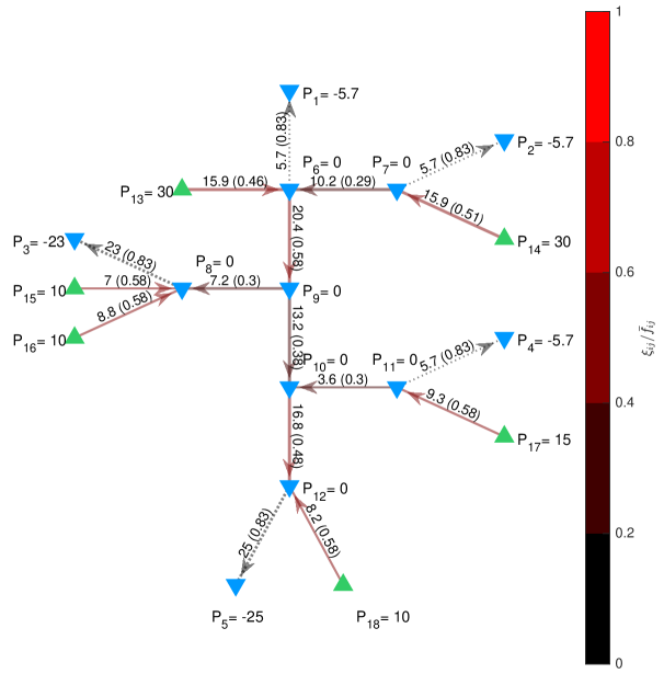
Figure 7: Microgrid topology used in Section 6.3, with active power values expressed in kW. Upward green triangles are generators, while downward blue triangles are loads. Dotted edges are those in $\mathcal{E}\setminus\mathcal{E}_{\mathrm{cf}}$. The values of the power flows $\xi_{ij}$ are the optimal ones with respect to (3.2), computed with the Matlab minimax function, and are reported on the edges. The fractions $\left\lvert\xi_{ij}\right\rvert/\bar{f}_{ij}$ are reported in brackets and the colors of the edges are a measure of proximity to failure.

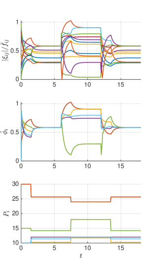
Figure 8: Results obtained when applying a centralized solution to (6.3). In the top panel, different colors represent $|\xi_{ij}|/\bar{f}_{ij}$ for different edges, with $\{i,j\}\in\mathcal{E}_{\mathrm{cf}}$. In the middle and bottom panels, different colors represent $\hat{\phi}_{i}$ and $P_{i}$ for different supplier nodes, i.e., $i\in\mathcal{V}_{\mathrm{s}}$.

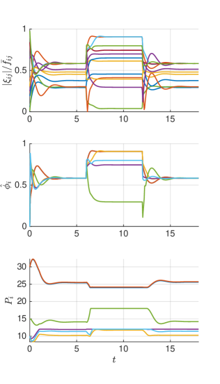
Figure 9: Results obtained when using the distributed online control strategy (6.5d).

Conclusion

We studied the minimax flow problem on acyclic networks showing that, by introducing the notion of maximum downstream flows, it can be reformulated as the problem of achieving their consensus. We then proposed a distributed estimation strategy to evaluate maximum downstream flows. We applied our results to the problem of preventing overcurrents in a droop-controlled AC microgrid via a distributed control strategy based on our approach. Our numerical experiments show that the distributed strategy is at least as effective, or even better, than the more traditional centralized solution strategy.

Extension to cyclic graphs

Future research will address the extension of the approach to solve minimax flow problems on cyclic networks. This is particularly important in applications such as transmission grids where the network can have a meshed structure. In this paper, the assumption that the graph is acyclic (i) implies that the maximum downstream flow (MDF) of a supplier quantifies how much that node is contributing to network congestion, and (ii) is used to allow distributed computation of the MDFs. Then, leveraging (i), the minimax flow problem is solved by balancing the MDFs. The main challenge associated with extending the results presented here to cyclic graphs will be to design quantities analogous to the MDFs that satisfy these two properties.

References

- [1] A. R. Bergen and D. J. Hill, “A structure preserving model for power system stability analysis,” IEEE Transactions on Power Apparatus and Systems, vol. 100, no. 1, pp. 25–35, 1981.
- [2] J. Burgschweiger, B. Gnädig, and M. C. Steinbach, “Optimization models for operative planning in drinking water networks,” Optimization and Engineering, vol. 10, no. 1, pp. 43–73, 2009.
- [3] E. Lovisari, G. Como, and K. Savla, “Stability of monotone dynamical flow networks,” in IEEE Conference on Decision and Control, Los Angeles, CA, USA, 2014, pp. 2384–2389.
- [4] S. L. Hakimi, “Optimum locations of switching centers and the absolute centers and medians of a graph,” Operations Research, vol. 12, no. 3, pp. 450–459, 1964.
- [5] M. E. O’Kelly and H. J. Miller, “Solution strategies for the single facility minimax hub location problem,” Papers in Regional Science, vol. 70, no. 4, pp. 367–380, 1991.
- [6] A. M. Campbell, T. J. Lowe, and L. Zhang, “Upgrading arcs to minimize the maximum travel time in a network,” Networks, vol. 47, no. 2, pp. 72–80, 2006.
- [7] P. L. Hammer, “Time-minimizing transportation problems: Time-minimizing transportation,” Naval Research Logistics Quarterly, vol. 16, no. 3, pp. 345–357, 1969.
- [8] R. S. Garfinkel and M. R. Rao, “The bottleneck transportation problem,” Naval Research Logistics Quarterly, vol. 18, no. 4, pp. 465–472, 1971.
- [9] T. Ichimori, H. Ishil, and T. Nishida, “Finding the weighted minimax flow in a polynomial time,” Journal of the Operations Research Society of Japan, vol. 23, no. 3, pp. 268–272, 1980.
- [10] R. K. Ahuja, “Algorithms for the minimax transportation problem,” Naval Research Logistics Quarterly, vol. 33, no. 4, pp. 725–739, 1986.
- [11] A. Nedić and J. Liu, “Distributed optimization for control,” Annual Review of Control, Robotics, and Autonomous Systems, vol. 1, no. 1, pp. 77–103, 2018.
- [12] B. Gharesifard and J. Cortés, “Distributed convergence to Nash equilibria in two-network zero-sum games,” Automatica, vol. 49, no. 6, pp. 1683–1692, 2013.
- [13] S. Yang, J. Wang, and Q. Liu, “Cooperative–competitive multiagent systems for distributed minimax optimization subject to bounded constraints,” IEEE Transactions on Automatic Control, vol. 64, no. 4, pp. 1358–1372, 2019.
- [14] A. Jadbabaie, A. Ozdaglar, and M. Zargham, “A distributed Newton method for network optimization,” in Proceedings of the 48h IEEE Conference on Decision and Control (CDC) held jointly with 2009 28th Chinese Control Conference. Shanghai, China: IEEE, 2009, pp. 2736–2741.
- [15] M. Zargham, A. Ribeiro, A. Ozdaglar, and A. Jadbabaie, “Accelerated dual descent for network flow optimization,” IEEE Transactions on Automatic Control, vol. 59, no. 4, pp. 905–920, 2014.
- [16] S. Z. Anaraki and M. Kalantari, “Acceleration of distributed minimax flow optimization in networks,” in Annual Conference on Information Sciences and Systems. Baltimore, MD, USA: IEEE, 2011, pp. 1–5.
- [17] A. A. Memon and K. Kauhaniemi, “A critical review of AC microgrid protection issues and available solutions,” Electric Power Systems Research, vol. 129, pp. 23–31, 2015.
- [18] A. Hooshyar and R. Iravani, “Microgrid protection,” Proceedings of the IEEE, vol. 105, no. 7, pp. 1332–1353, 2017.
- [19] S. A. Hosseini, H. A. Abyaneh, S. H. H. Sadeghi, F. Razavi, and A. Nasiri, “An overview of microgrid protection methods and the factors involved,” Renewable and Sustainable Energy Reviews, vol. 64, pp. 174–186, 2016.
- [20] M. Khederzadeh, “Identification and prevention of cascading failures in autonomous microgrid,” IEEE Systems Journal, vol. 12, no. 1, p. 8, 2018.
- [21] P. Nahata, S. Mastellone, and F. Dörfler, “A decentralized switched system approach to overvoltage prevention in PV residential microgrids,” IFAC-PapersOnLine, vol. 50, no. 1, pp. 6630–6635, 2017.
- [22] M. Goyal, A. Ghosh, and F. Shahnia, “Overload prevention in an autonomous microgrid using battery storage units,” in IEEE PES General Meeting, National Harbor, MD, USA, 2014.
- [23] A. H. Etemadi, E. J. Davison, and R. Iravani, “A decentralized robust control strategy for multi-DER Microgrids—Part I: Fundamental concepts,” IEEE Transactions on Power Delivery, vol. 27, no. 4, pp. 1843–1853, 2012.
- [24] J. Shah, B. F. Wollenberg, and N. Mohan, “Decentralized power flow control for a smart micro-grid,” in 2011 IEEE Power and Energy Society General Meeting, San Diego, CA, 2011, pp. 1–6.
- [25] Niannian Cai and J. Mitra, “A decentralized control architecture for a microgrid with power electronic interfaces,” in North American Power Symposium 2010, Arlington, TX, USA, 2010, pp. 1–8.
- [26] S. Anand and B. G. Fernandes, “Reduced-order model and stability analysis of low-voltage DC microgrid,” IEEE Transactions on Industrial Electronics, vol. 60, no. 11, pp. 5040–5049, 2013.
- [27] Y. Gu, X. Xiang, W. Li, and X. He, “Mode-adaptive decentralized control for renewable DC microgrid with enhanced reliability and flexibility,” IEEE Transactions on Power Electronics, vol. 29, no. 9, pp. 5072–5080, 2014.
- [28] J. W. Simpson-Porco, F. Dörfler, and F. Bullo, “Synchronization and power sharing for droop-controlled inverters in islanded microgrids,” Automatica, vol. 49, no. 9, pp. 2603–2611, 2013.
- [29] C. Bersani, H. Dagdougui, A. Ouammi, and R. Sacile, “Distributed robust control of the power flows in a team of cooperating microgrids,” IEEE Transactions on Control Systems Technology, vol. 25, no. 4, pp. 1473–1479, 2017.
- [30] T. Ichimori, H. Ishii, and T. Nishida, “Weighted minimax real-valued flows,” Journal of the Operations Research Society of Japan, vol. 24, no. 1, pp. 52–60, 1981.
- [31] R. Penrose, “A generalized inverse for matrices,” Mathematical Proceedings of the Cambridge Philosophical Society, vol. 51, no. 3, pp. 406–413, 1955.
- [32] F. Dörfler, M. Chertkov, and F. Bullo, “Synchronization in complex oscillator networks and smart grids,” Proceedings of the National Academy of Sciences, vol. 110, no. 6, pp. 2005–2010, 2013.
- [33] F. Bullo, Lectures on Network Systems, 1.6 ed. Kindle Direct Publishing, 2022.
- [34] S. Parhizi, H. Lotfi, A. Khodaei, and S. Bahramirad, “State of the art in research on microgrids: A review,” IEEE Access, vol. 3, pp. 890–925, 2015.
- [35] S. V. Iyer, M. N. Belur, and M. C. Chandorkar, “A generalized computational method to determine stability of a multi-inverter microgrid,” IEEE Transactions on Power Electronics, vol. 25, no. 9, pp. 2420–2432, 2010.
- [36] S. Papathanassiou, N. Hatziargyriou, and K. Strunz, “A benchmark low voltage microgrid network,” in Proceedings of the CIGRE Symposium: Power Systems with Dispersed Generation, 2005, pp. 1–8.
- [37] MATLAB, Version 9.9.0.1524771 (R2020b) Update 2. Natick, Massachusetts: The MathWorks Inc., 2021.