Fast optimal structures generator for parameterized quantum circuits

Abstract

Current structure optimization algorithms optimize the structure of quantum circuit from scratch for each new task of variational quantum algorithms (VQAs) without using any prior experience, which is inefficient and time-consuming. Besides, the number of quantum gates is a hyper-parameter of these algorithms, which is difficult and time-consuming to determine. In this paper, we propose a rapid structure optimization algorithm for VQAs which automatically determines the number of quantum gates and directly generates the optimal structures for new tasks with the meta-trained graph variational autoencoder (VAE) on a number of training tasks. We also develop a meta-trained predictor to filter out circuits with poor performances to further accelerate the algorithm. Simulation results show that our method output structures with lower loss and it is 70$\times$ faster in running time compared to a state-of-the-art algorithm, namely DQAS.

I Introduction

Variational quantum algorithmCerezo et al. (2021) (VQA) is one of the most promising strategies to achieve quantum advantage and has been applied successfully to problems of optimization Farhi et al. (2014); Wang et al. (2018); Crooks (2018), quantum chemistryPeruzzo et al. (2014); McClean et al. (2016); Williams-Noonan et al. (2018); Heifetz (2020) and quantum machine learning modelsBiamonte et al. (2017); Romero et al. (2017); Farhi and Neven (2018); Mitarai et al. (2018); Du et al. (2020a); Situ et al. (2020). The performances of VQAs rely largely on the structures of parameterized quantum circuits. Many VQAs use manually-designed structures, which depend heavily on human experts and are inefficient. Some VQAs use structure templates Kandala et al. (2017); Hadfield et al. (2019), which are inflexible and have many redundant gates.

Structure optimization algorithms (SOAs) have been proposed to search automatically an optimal circuit structure for a given variational quantum algorithm Khatri et al. (2019); Li et al. (2020); Lu et al. (2021); Zhang et al. (2020, 2021); He et al. (2021); Moro et al. (2021); Ostaszewski et al. (2021); Kuo et al. (2021); Du et al. (2020b). However, current SOAs search an optimal circuit structure according to a predefined circuit length. The circuit length is a hyperparameter, which is given by the prior knowledge of human experts or the simulation results of different lengths. VQA cannot converge to the optimal solution when the length of the quantum circuit is insufficient. However, there exist a lot of redundant gates resulting in many noises if the circuit length is too large. Exploring an optimal length would be computationally expensive.

Most of SOAs optimize the circuit structure from scratch for each new task without using any prior experience. A MetaQAS algorithmChen et al. (2021) is proposed to accelerate SOAs by using prior experience of the optimal structures in the past tasks. However, MetaQAS only learns the initialization heuristics of the structure and gate parameters for the circuit with a fixed length. It needs still further optimizations on its structure and gate parameters.

To deal with the above problems, we propose a rapid structure optimization algorithm for VQAs, which can generate directly quantum circuits with optimal lengths and structures with respect to a given new task by a meta-trained generator. The structure of the quantum circuit is denoted by a directed acyclic graph (DAG) Nam et al. (2018); Childs et al. (2019); Wu et al. (2020a). We train a DAG variational autoencoder (VAE) on a variety of VQA tasks and their corresponding optimal structures. For a given new tasks, the trained VAE can directly generate the optimal structures. We also train a predictor on the performances of different structures on different VQA tasks to directly filter out the structures with poor performances. It is worth to point out that the training of the generator and predictor is a one time job and can be applied to a variety of new tasks. Simulation results show that the proposed method can generate better structures than a state-of-the-art algorithm, i.e., DQAS Zhang et al. (2020). Moreover, it is 70$\times$ faster than DQAS.

II Method

We propose a rapid structure optimization algorithm for parameterized quantum circuits by using the prior knowledge attained from a variety of training tasks. The proposed method can be used to generate the optimal circuit structures for tasks of different VQAs. In this section, we illustrate how to generate the optimal quantum circuits for the tasks of variational quantum compiling, which is a typical VQA. Quantum compiling aims to convert a target quantum circuit or unitary $U_{t}$ into a native gate sequence $U_{c}(\bm{\theta})$, where $\bm{\theta}$ is the trainable gate parameters of the compiled circuit.

We use a directed acyclic graph (DAG) $\mathcal{G}$ to represent a quantum circuit, where the nodes of the DAG denote the quantum gates and the directed edges encode their input/output relationships. A note $v$ can be denoted by $\mathit{GATE}\textendash{q_{i}}$, where $\mathit{GATE}$ is the type of the quantum gate and ${q_{i}}$ is the qubit that the gate operates on. For example, $\mathit{R_{x}}\textendash q_{2}$ denotes a rotation gate $R_{x}$ acting on the qubit $q_{2}$. By representing an $N$-qubits quantum circuit with a DAG, we add a $\mathit{Start}\textendash{\{q_{i}\}_{i=1}^{N}}$ and an $\mathit{End}\textendash{\{q_{i}\}_{i=1}^{N}}$ nodes as the first and the last nodes of the DAG. Fig. 1 shows an example of the DAG representation of a quantum circuit, whose length ($L$) and depth ($D$) are $5$ and $4$. The DAG has 7 nodes including a Start and an End nodes. The DAG naturally contains the structure information of the quantum circuit such as the type of quantum gates and their connection relationships. By using the DAG representation, we can extract the structure information of a quantum circuit with graph modelsHamilton et al. (2017); Wu et al. (2020b).

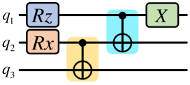
(a) a quantum circuit with $5$ gates

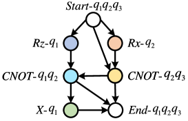
(b) DAG representation of the quantum circuit

Figure 1: An example of the DAG representation of a quantum circuit.

The proposed method consists of two steps, i.e., training and test steps, as shown in Fig. 2. During the training step, we train a generator on a variety of tasks $\mathcal{D}=\{(\mathcal{G}_{t_{i}},\mathcal{G}_{c_{i}})\}_{i=1}^{N_{\tau}}$ with meta-learning, where $N_{\tau}$ is the number of training tasks. Each task consists of a target circuit $\mathcal{G}_{t_{i}}$ and its compiled circuit $\mathcal{G}_{c_{i}}$. The target circuits are randomly generated and their corresponding compiled circuits can be found by any structure optimization algorithm. The generator consists of a graph encoder ($q_{\bm{\phi}}(\mathbf{z}\mid\mathcal{G}_{t})$) and a graph decoder ($p_{\bm{\varphi}}(\mathcal{G}_{c}\mid\mathbf{z})$ ), which are used to learn a latent space ($\mathcal{Z}$) between the target circuits and the compiled ones via amortized inference, where $\bm{\phi}$ and $\bm{\varphi}$ are trainable parameters of the graph encoder and decoder. We meta-train the generator to minimize the approximated evidence lower bound (ELBO) for each task using amortized inference

$$\min_{\bm{\phi,\varphi}}\sum_{(\mathcal{G}_{t},\mathcal{G}_{c})\sim\mathcal{D}}(-\mathds{E}_{\mathbf{z}\sim q_{\bm{\phi}}\left(\mathbf{z}\mid\mathcal{G}_{t}\right)}(\log p_{\bm{\varphi}}\left(\mathcal{G}_{c}\mid\mathbf{z}\right))+\lambda\cdot\operatorname{KL}(q_{\bm{\phi}}\left(\mathbf{z}\mid\mathcal{G}_{t}\right)\|p(\mathbf{z}))).$$ (1)

The first term is the reconstructed loss and the latter is Kullback-Leibler(KL) divergence between two distributions. We make $q_{\bm{\phi}}(\mathbf{z}\mid\mathcal{G}_{t})$ close to the prior distribution $p(\mathbf{z})$ by minimizing the KL divergence, where $p(\mathbf{z})$ is a standard normal distribution. $\lambda$ is a weighted parameter which balances the reconstructed and KL loss. The optimization problem can be solved by stochastic gradient variational BayesKingma and Welling (2013). During the meta-training, we use the teacher forcing strategy Jin et al. (2018) to calculate the reconstructed loss.

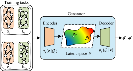
(a) training step

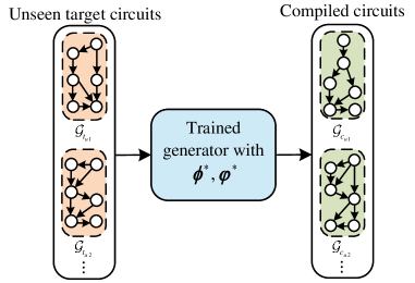
(b) test step

Figure 2: The workflow of the proposed method.

In the test phase, we can use the meta-trained generator to directly generate compiled circuits for new target circuits which are different from the training ones. Given a new target circuit, we use the graph encoder $q_{\bm{{\phi}^{*}}}(\mathbf{z}\mid\mathcal{G}_{t})$ to calculate its latent vector $\mathbf{z}$. The decoder $p_{\bm{{\varphi}^{*}}}(\mathcal{G}_{c}\mid\mathbf{z})$ generates serval candidates of compiled quantum circuits based on $\mathbf{z}$ according to Algorithm 1. Then we can select the candidate with the lowest cost after fine-tuning the gate parameters as the final compiled circuit. We describe the encoder, decoder and predictor in detail in the following.

II.1 Encoder

The encoder $q_{\bm{\phi}}(\mathbf{z}\mid\mathcal{G}_{t})$ encodes the target circuit represented by a DAG $\mathcal{G}_{t}$ into a latent code $\mathbf{z}$. We use a graph neural network to compute the hidden state $\mathbf{h}_{v}$ of each node $v$ in $\mathcal{G}_{t}$ as shown in Fig. 3(a)

$$\mathbf{h}_{v}=\mathcal{U}\left(\mathbf{x}_{v},\mathbf{h}_{v}^{\text{in}}\right),$$ (2)

where $\mathcal{U}$ is an update function which can be implemented by a Gated Recurrent Unit (GRU) model Chung et al. (2014)

$$\mathbf{h}_{v}=\mathit{GRU}_{e}\left(\mathbf{x}_{v},\mathbf{h}_{v}^{\text{in}}\right).$$ (3)

$\mathbf{x}_{v}$ is a one-hot vector of the node $v$, which represents a candidate operation considering the type of the quantum gate and the qubit it acts on. $\mathbf{h}_{v}^{\mathrm{in}}=\mathcal{A}\left(\left\{\mathbf{h}_{u}:u\rightarrow v\right\}\right)$, where $\mathcal{A}$ is an aggregation function and $u\rightarrow v$ denotes that there is a directed edge from the node $u$ to the node $v$. $\{\mathbf{h}_{u}:u\rightarrow v\}$ is a set of hidden states of $v$’s predecessors. The aggregation function $\mathcal{A}$ can be implemented by a gated sum function

$$\mathbf{h}_{v}^{\text{in}}=\sum_{u\rightarrow v}g_{e}\left(\mathbf{h}_{u}\right)\odot m_{e}\left(\mathbf{h}_{u}\right),$$ (4)

where $g_{e}$ is a gating network which is a single linear layer followed by a $sigmoid$ activation function. $m_{e}$ is a mapping network which is a single linear layer without bias and activation function. $\odot$ is element-wise multiplication. We set $\mathbf{h}_{v}^{\text{in}}$ of the $\mathit{Start}$ node to be a zero vector, which has no predecessor node. The hidden state of the $\mathit{End}$ node is used to represent the graph state, i.e., $\mathbf{h}_{\mathcal{G}_{t}}=\mathbf{h}_{v_{End}}$.

We take $\mathbf{h}_{\mathcal{G}_{t}}$ as the input of two single linear layers $\mathrm{NN}_{\bm{\mu}}$ and $\mathrm{NN}_{\bm{\sigma}}$ to obtain the mean vector $\bm{\mu}$ and standard deviation vector $\bm{\sigma}$ as shown in Fig. 3(a). Then the hidden vector $\mathbf{z}$ can be sampled from a circuit-conditioned Gaussian distribution, i.e., $\mathbf{z}\sim q_{\bm{\phi}}\left(\mathbf{z}\mid\mathcal{G}_{t}\right)=\mathcal{N}(\bm{\mu},\bm{\sigma}^{2})$. By using the reparameterization trick, $\mathbf{z}$ can be denoted as $\mathbf{z}=\bm{\mu}+\bm{\sigma}\odot\bm{\epsilon}$, where $\bm{\epsilon}\sim\mathcal{N}(\mathbf{0},\mathbf{I})$. The latent vector $\mathbf{z}$ is an embedding of $\mathcal{G}_{t}$ in the latent space $\mathcal{Z}$, which is the input of the decoder.

II.2 Decoder

Given a latent vector, the graph decoder $p_{\bm{{\varphi}}}(\mathcal{G}\mid\mathbf{z})$ outputs a DAG $\mathcal{G}$ which represents a quantum circuit. The detailed process is shown in Algorithm 1. A single linear layer $\mathrm{NN}_{init}$ with $\mathit{tanh}$ activity function is used to calculate the hidden state of the $\mathit{Start}$ node $v_{0}$. Then the hidden state of the subsequent node $v_{i}$ is calculated by $\mathit{GRU}_{d}$, $g_{d}$ and $m_{d}$, which have the same structures with $\mathit{GRU}_{e}$, $g_{e}$ and $m_{e}$ used in the encoder. We progressively sample and add a new node $v_{i+1}$ to $\mathcal{G}$ based on the probability distribution determined by the hidden state of its last note $v_{i}$, i.e., $\bm{p}=f_{p}(\mathbf{h}_{v_{i}})$, until an $End$ node is sampled or the circuit length reaches the defined maximum length, where $f_{p}$ is a single linear layer followed by a $\mathit{softmax}$ function.

Algorithm 1 DAG generation with a decoder.

1:$\mathbf{z}$: a latent vector.

2:$\mathcal{G}$ ={}, $i=0$ and add a $Start$ node to $\mathcal{G}$.

3:calculate the hidden state of the $Start$ node $\mathbf{h}_{0}=\mathrm{NN}_{init}(\mathbf{z})$.

4:repeat

5:     calculate the hidden state $\mathbf{h}_{v_{i}}$ of the node $v_{i}$ using $\mathit{GRU}_{d}$, $g_{d}$ and $m_{d}$.

6:     sample and add the next node $v_{i+1}$ to $\mathcal{G}$ based on the probability distribution $\bm{p}=f_{p}(\mathbf{h}_{v_{i}})$.

7:     add directed edge to $v_{i+1}$ according to the operated qubits of the selected gate.

8:     $i=i+1$

9:until $v_{i}$ is an $End$ node or the circuit length reaches the maximum length

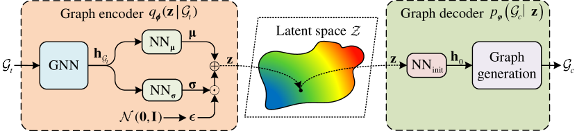
(a) generator

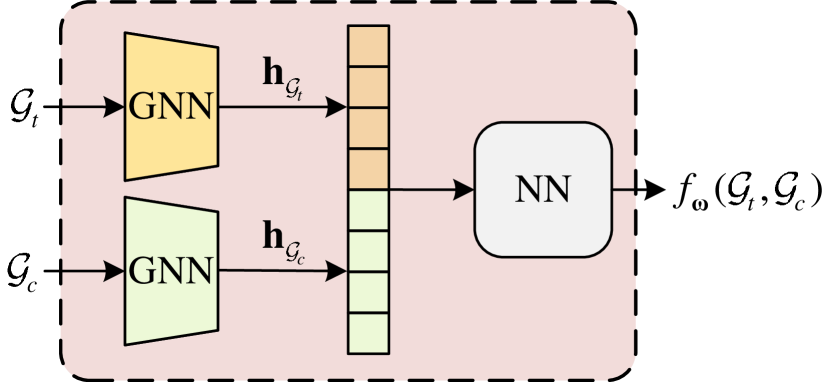
(b) predictor

Figure 3: The structures of the generator and the predictor.

II.3 Predictor

Current SOAs require to evaluate the performances of a large number of circuit structures on NISQ devises, which requires a large amount of running time. Zhang et al. trained a neural predictor with a small subset of quantum circuits to estimate the performances of different structuresZhang et al. (2021). The predictor is trained for a specific task and requires to retrain for a new task.

A meta-trained predictor on a variety of tasks $\mathcal{D}_{pre}$ can directly predict the performances of quantum circuits for different unseen tasks instead of getting the loss on the quantum devices after optimizing its gate parameters, which can significantly reduce the evaluation time of circuit structures. Each training sample consists of a target circuit, a compiled circuit and the corresponding loss, which are represented by $\mathcal{G}_{t}$, $\mathcal{G}_{c}$ and $s$. The structure of the predictor is described in Fig. 3(b). The DAGs $\mathcal{G}_{t}$ and $\mathcal{G}_{c}$ are first converted to hidden vectors $\mathbf{h}_{\mathcal{G}_{t}}$ and $\mathbf{h}_{\mathcal{G}_{c}}$ by two graph neural networks, whose structures are the same as the one used in the encoder. $\mathbf{h}_{\mathcal{G}_{t}}$ and $\mathbf{h}_{\mathcal{G}_{c}}$ are feeded into two linear layers with $\mathit{relu}$ to get the predicted loss $f_{\bm{\omega}}(\mathcal{G}_{t},\mathcal{G}_{c})$, where $\bm{\omega}$ are the trainable parameters of the predictor. The predictor are trained by minimizing the Mean-Squared Loss between the predicted loss and the true one

$$\min_{\bm{\omega}}\sum_{(\mathcal{G}_{t},\mathcal{G}_{c},s)\sim\mathcal{D}_{pre}}\left(s-f_{\bm{\omega}}(\mathcal{G}_{t},\mathcal{G}_{c})\right)^{2}.$$ (5)

III Numerical simulation

In this section, we show the simulation results of the meta-trained generator and predictor on variational quantum compiling, and compare the performance of the proposed method to a state-of-the-art structure optimization algorithm, i.e., DQAS Zhang et al. (2020). All the simulations are run on a classical computer with a CPU i9-10900K. We consider target circuits with 3 qubits. The target circuits consist of 4, 5 or 6 quantum gates which are randomly selected from the gate set $\mathcal{A}_{\mathit{target}}=${$\mathit{H}$, $\mathit{PauliX}$, $\mathit{PauliY}$, $\mathit{PauliZ}$, $\mathit{S}$, $\mathit{T}$, $\mathit{R_{X}}(\theta)$, $\mathit{R_{Y}}(\theta)$, $\mathit{R_{Z}}(\theta)$, $\mathit{CNOT}$, $\mathit{CZ}$, $\mathit{CY}$, $\mathit{SWAP}$, $\mathit{Toffoli}$, $\mathit{CSWAP}$} and act on randomly selected qubits. The training dataset of the generator contains 3000 samples and each sample consists of the DAGs of the target and the compiled circuits. The native gate set for variational quantum compiling is $\mathcal{A}_{\mathit{native}}=${$\mathit{RX}(\pi,\pm\pi/2)$, $\mathit{RZ}(\theta)$, $\mathit{CRZ}(\theta)$, $\mathit{CZ}$, $\mathit{XY}(\theta)$}, which is used by Rigetti’s Aspen-11 quantum processor Asp . We set the maximum length of the compiled circuit to 30. The generator is trained until the loss converges, which takes 1.57 hours.

After training, we evaluate the generator with 300 target circuits which do not exist in the training dataset. For each test circuit, the generator generates 100 structures of the compiled circuit. We get the LHST loss Khatri et al. (2019) of each structure after its gate parameters are optimized, and output the one with the lowest loss. As described in Section II.2, the graph decoder generates a circuit by sequentially choosing candidate gates from the native gate set based on the probability distribution of candidate gates. We consider different sampling strategies , including stochastic and top-$k$ sampling schemes Fan et al. (2018), where $k=10,15,20,25$. Stochastic and top-$k$ sampling means that the decoder selects candidate gates according to the probability distribution of all the candidate gates and the $k$ candidate gates with the highest probabilities.

We show the average loss of the proposed method in Tabel 1. We also show the length ($L$) and the depth ($D$) of the compiled circuits, which are defined as the number of quantum gates and the number of layers, respectively. The stochastic scheme achieves the lowest loss. However, its compiled circuits use more quantum gates and have a larger depth. For the top-$k$ scheme, the loss decreases with the increasing of $k$. More gates are used in the compiled circuit for a larger $k$. However, the depths of compiled circuits with different $k$ are similar. The top-$k$ scheme makes a balance between the loss and the depth of the circuit. In the following simulations, we use top-$25$ scheme.

Table 1: The average loss of compiling 300 target circuits with the proposed generator.

Strategy	Loss	$L$	$D$	Uniqueness (%)	Novelty (%)
Top-10	0.0333	14.94	12.30	99.96	100.00
Top-15	0.0205	16.33	12.73	99.99	100.00
Top-20	0.0153	16.50	12.42	99.99	100.00
Top-25	0.0133	17.01	12.28	99.99	100.00
Stochastic	0.0071	24.78	16.09	97.71	100.00

We also show the uniqueness and the novelty of the generated circuits in Table 1, which are defined as the percentage of unique circuits in the generated circuits and the percentage of circuits that do not exist in the training set. The quantum circuits generated by different sampling schemes have a very low repeatability and the novelty is 100.00%, which demonstrates the good capability of the proposed model to generate optimal quantum circuits for different tasks, rather than just simply copying the circuits from the training set.

In previous simulations, we assumed that the qubits are fully connected. However, the qubits are not fully connected in the NISQ era. We consider the chain connection, $i.e.$, ${q_{1}}\textendash{q_{2}}\textendash{q_{3}}$ and use the meta-trained generator to generate circuits under limited connections. The search space in the chain connection is a subspace of the fully connected one. There is no need to recollect training data and retrain the generator. Instead, we can simply add a mask code which forces the generator to only choose permitted operations under limited connections. The simulation results on chain connection is shown in Table 2. The average losses under limited connections are similar to those under fully connections. As the connection between ${q_{1}}$ and ${q_{3}}$ is forbidden, it requires more gates and larger depth.

Table 2: The average losses of compiling 300 target circuits with the proposed generator under limited connections.

Strategy	Loss	$L$	$D$
Top-10	0.0316	15.46	12.73
Top-15	0.0201	16.48	13.07
Top-20	0.0155	17.46	12.99
Top-25	0.0144	17.71	12.96
Stochastic	0.0070	25.49	16.42

We train a predictor to accelerate the proposed method by removing the generated circuits with unsatisfying performance. The training dataset consists of 200,000 samples and each sample contains the DAGs of a target and its compiled circuit as well as the corresponding loss. Please see Appendix D for more details of the training and test dateset. The predictor is trained for 100 epochs. The Pearson correlation coefficient between the predicted and the true loss on 10,000 test samples is 0.784, which indicates a strong correlation between the predicted loss and the true one. For ease of visualization, we illustrate the predicted and true losses of 1,000 randomly selected test samples in Fig. 4.

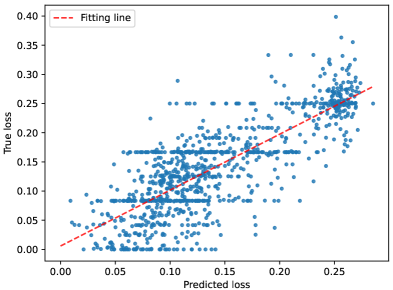
Figure 4: The relationship between the predicted loss and the ground-truth one.

We show the loss distributions of 10,000 test samples and the remaining samples after removing the ones whose predicted losses are larger than 0.1 in Fig. 5. We can observe that the predictor can filter out most of compiled circuits with poor performances while retain circuits with high performances.

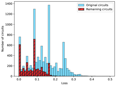
Figure 5: The loss distributions of 10,000 test samples (blue bars) and the remaining samples filtered by the predictor (red bars).

We compare the performance of the proposed method with a state-of-the-art structure optimization algorithm, namely DQAS Zhang et al. (2020), in terms of loss and running time. As the circuit length $L$ is a hyperparameter of DQAS, we gradually increase $L$ until the loss is less than 0.05 or the circuit length reaches 30. The simulation results are shown in the Table 3 and Table 4. The proposed methods achieve lower losses than DQAS. The average length and depth of the proposed methods with top-25 scheme are similar to the ones of DQAS. By using stochastic scheme, the proposed method achieves the lowest loss, i.e., 0.0075. However, it uses 8 more gates, leading to a 4 increase in depth. The loss, length and depth of the proposed method with a predictor is similar to the one without predictor.

Table 3: Simulation results of different structure optimization algorithms. “gen” and “pred” denote the generator and predictor, respectively.

Method	Loss	$L$	$D$
DQASZhang et al. (2020)	0.0269	17.44	12.27
Gen-top-25	0.0141	17.02	12.36
Gen-stochastic	0.0075	25.01	16.39
Gen-pred-top-25	0.0150	17.69	12.92
Gen-pred-stochastic	0.0086	26.81	17.54

Tabel 4 shows the running time of different structure optimization algorithms. We define the times of searching the optimal structures and fine-tuning the gate parameters as $t_{s}$ and $t_{f}$, respectively. The running time of the predictor is denoted as $t_{p}$. $t_{total}$ shows the total running time of each algorithm. DQAS takes 8.4 hours to search the optimal structure while the proposed method only need about 1 second to generate compiled circuits. The running time of fine-tuning step in our method is higher than DQAS as we need to fine-tune the gate parameters of a set of generated circuits. The total running times of the proposed method with top-25 and stochastic schemes are 13.35 and 15.15 minutes, which are only 2.6% and 3.0% of that used by DQAS. The predictor takes less than haft a second to predict the performances of different generated circuits. By filtering out the generated circuits with poor performances, we can largely reduce the running times in the fine-tuning step, which reduces the total running time by half.

Table 4: Running times of compiling 90 target circuits with different structure optimization algorithms.

Method	$t_{s}$	$t_{p}$	$t_{f}$	$t_{total}$
DQASZhang et al. (2020)	8.36 (h)	/	2.66(min)	8.40(h)
Gen-top-25	0.98(s)	/	13.31(min)	13.35(min)
Gen-stochastic	1.05(s)	/	15.13(min)	15.15(min)
Gen-Pred-top-25	0.98(s)	0.36(s)	7.08(min)	7.10(min)
Gen-Pred-stochastic	1.05(s)	0.40(s)	6.95(min)	6.98(min)

IV Conclusion

In this paper, we proposed to generate directly optimal circuits for new tasks with a meta-trained graph variational autoencoder on a variety of training tasks. Numerical experimental results on variational quantum compiling showed that the proposed algorithm can generate quantum circuits with similar performance as the DQAS algorithm while taking only 2.6% of its running time. We also proposed a predictor to filter out the structures with unsatisfying performances, which can reduce the total running time by 50%. We will apply the proposed algorithm to other VQAs, e.g., Variational Quantum Eigensolver (VQE) and Quantum Approximate Optimization Algorithm (QAOA) in future works.

Appendix A Hyperparameters in simulations

We implement the simulations on a classical computer with a CPU i9-10900K using PennylaneBergholm et al. (2018), which includes a wide range of quantum machine learning libraries. The generator and the predictor are trained with Adam optimizerKingma and Ba (2014). The hyperparameters of the proposed method and DQAS are shown in Table 5 and Table 6.

Table 5: The hyperparameters of the our method.

Hyperparameters		Value
	Dimenstion of $\mathbf{h}_{v}$	56
	Dimenstion of $\mathbf{z}$	56
	Batch size of meta-training	32
	Learning rates for training the generator and predictor	1e-4
	Weighted parameter $\lambda$	1e-5
	Number of training epochs for the generator	400
	Number of training epochs for the predictor	100

Table 6: The hyperparameters of DQAS.

Hyperparameter	Value
Batch size	256
Number of training epochs	300
Learning rate of the structure	0.2
Learning rate of the gate parameters	0.1

Appendix B Details of graph computation

In order to extract the structure information from the DAG $\mathcal{G}$ more accurately, we use a bidirectional encoding strategy Zhang et al. (2019), which computes the graph state in both the forward and backward directions. Specifically, we use two GRUs to obtain the forward and the backward graph states ($\bm{h}_{f}$ and $\bm{h}_{b}$), respectively. We concatenate $\bm{h}_{f}$ and $\bm{h}_{b}$ and use a trainable single linear layer to reduce the dimension of the concatenated vector by half. We use this vector to denote the final graph state $\bm{h}_{\mathcal{G}}$. The position information of the previously connected nodes is also considered in the calculation of $\mathbf{h}_{v}$

$$\mathbf{h}_{v}^{\text{in}}=\sum_{u\rightarrow v}g\left(\mbox{Concat}(\mathbf{h}_{u},\mathbf{x}_{\text{pos}})\right)\odot m\left(\mbox{Concat}(\mathbf{h}_{u},\mathbf{x}_{\text{pos}})\right),$$ (6)

where $\mathbf{x}_{\text{pos}}$ is a one-hot vector of the node $u$’s global position.

Appendix C Training dataset of the generator

Each training sample of the generator consists of a target circuit and the optimal compiled one with the native gates. The training set consists of target circuits with different lengths, i.e., $L=4,5,6$. We randomly generate 1000 target circuits for each length , leading to 3000 target circuits in the training set. In this paper, we use the DQAS algorithm Zhang et al. (2020) to search the optimal compiled circuits of the target circuits. It should be noted that any other QAS algorithm can be used to search the optimal compiled circuits. We search the compiled circuit for each target circuit by gradually increasing the length of the compiled circuit until the loss is lower than 0.05 or the circuit length reaches $5L$. If the loss of the compiled circuit with $5L$ gates is higher than 0.05, we will give up the corresponding target circuit as we cannot find a compiled circuit within a limited length.

Appendix D Training and test dataset of the predictor

Each training sample of the predictor consists of a target circuit $\mathcal{G}_{t_{i}}$, a compiled circuit $\mathcal{G}_{c_{i}}$ and the corresponding loss $s_{i}$. The training set of the predictor should include the compiled circuits with a variety of performances. We use the 3,000 training samples of the generator and calculate the corresponding losses. In addition, we also collect 207,000 target circuits which are generated by randomly selecting 4, 5 and 6 gates from $\mathcal{A}_{\mathit{target}}$ and randomly choosing the operated qubits. Their compiled circuits are generated by randomly selecting $[2L,5L]$ gates from $\mathcal{A}_{\mathit{native}}$ and randomly choosing the operated qubits, where $L$ is the number of quantum gates in the target circuit. The 210,000 samples are randomly divided into the training and test sets of the predictor, which consist of 200,000 and 10,000 samples, respectively.