Selecting the Best Optimizing System

Abstract

We formulate selecting the best optimizing system (SBOS) problems and provide solutions for those problems. In an SBOS problem, a finite number of systems are contenders. Inside each system, a continuous decision variable affects the system’s expected performance. An SBOS problem compares different systems based on their expected performances under their own optimally chosen decision to select the best, without advance knowledge of expected performances of the systems nor the optimizing decision inside each system. We design easy-to-implement algorithms that adaptively chooses a system and a choice of decision to evaluate the noisy system performance, sequentially eliminates inferior systems, and eventually recommends a system as the best after spending a user-specified budget. The proposed algorithms integrate the stochastic gradient descent method and the sequential elimination method to simultaneously exploit the structure inside each system and make comparisons across systems. For the proposed algorithms, we prove exponential rates of convergence to zero for the probability of false selection, as the budget grows to infinity. We conduct three numerical examples that represent three practical cases of SBOS problems. Our proposed algorithms demonstrate consistent and stronger performances in terms of the probability of false selection over benchmark algorithms under a range of problem settings and sampling budgets.

Keywords: Best optimizing system, probability of false selection, exponential rate, stochastic gradient descent, sequential elimination

1 Introduction

The need to select a system with the best mean system performance among a number of different systems naturally arises in various decision making problems. The decision maker is typically able to generate or collect unbiased noisy random samples of the expected performance for each system in contention. The task of selecting the best system in a statistically principled way, as an abstraction of many practical applications, is a fundamental research problem in several growing research areas. In the area of stochastic simulation, this research problem is referred to as Ranking and Selection or Selecting the Best System; see Kim and Nelson (2006), Chick (2006), Hunter and Nelson (2017) and Hong, Fan, and Luo (2021) for comprehensive reviews and see Chick and Wu (2005), Lan, Nelson, and Staum (2010), Waeber, Frazier, and Henderson (2010), Luo, Hong, Nelson, and Wu (2015), Fan, Hong, and Zhang (2020), Shen, Hong, and Zhang (2021) for various applications in healthcare decisions, production management, financial risk evaluation and decisions, etc. For most Selecting the Best System problems, noisy random samples are generated from running costly stochastic simulations, where the simulation model is often built to represent real complicated systems or new systems that have yet to be developed. The task of selecting the best system also appears in experimental designs for clinical trials or A/B testing (see Johari, Koomen, Pekelis, and Walsh (2021) and Chick, Gans, and Yapar (2021) for example), where the noisy random samples are collected from running costly treatment experiments on individuals. Both the Selecting the Best System literature and the clinical trials literature point back to Bechhofer (1954) and Bechhofer, Santner, and Goldsman (1995), and both literature aim at selecting the best or better system in a statistically principled way. The two literature share the same notion that samples are noisy and costly to generate or collect, despite of the difference on how the samples are generated or collected.

Most existing literature on selecting the best system (i.e., selecting a system with the best mean system performance) assumes that one has access to independent unbiased noisy samples of the system performance for each system in comparison. However, this access can be unavailable for problems where each system in comparison involves optimizing a decision inside the system. For instance, such a phenomenon arises in the following application examples.

• Medication and Healthcare. Suppose a pharmaceutical factory has designed two new drugs to treat insomnia symptom for some specific type of patients. The factory needs to run experiments to test the effects of the two new drugs and the decision is to select the best (better) one to massively produce, distribute, promote, and sell. In this example, each drug is a “system” corresponding to the problem of selecting the best system. For each drug, different doses can lead to different expected effects for the targeted patients (see for example Erman, Seiden, Zammit, Sainati, and Zhang (2006), Verweij, Danaietash, Flamion, Ménard, and Bellet (2020)). Therefore, when comparing two drugs (systems) and selecting the better one, the “system performance” is the expected effect of a drug at its optimal dose. That said, the dosage is often a continuous variable and what exact dosage is optimal for a drug may not be known a priori. Therefore, a challenge is that the decision maker has no access to an unbiased estimator for the optimizing expected effect for each drug. The task of selecting the best system (drug) naturally involves an inner layer of optimization to optimize the dosage amount inside each system.

• Simulation Optimization for Complex Stochastic Systems. For non-stationary service systems, a manager often uses simulation optimization to make staffing plans under resource constraints (e.g., a constraint on the total number of staff members). Suppose that a manager has $N$ staff members and needs to select a staffing plan that has the best expected system performance (where the performance metric may involve service revenue, total customer abandonment due to long waiting times, etc.). In this example, the service system under each staffing plan is a “system”. Within each system (which is, given each staffing plan), the manager also needs to make other decisions to improve the system performance. One example of such decision is to set a price for the service (Kim and Randhawa (2018), Lee and Ward (2019)). With a given objective function, for different staffing plans, the optimal price to set for the service may be different. In addition, what is the optimal price for each system (staffing plan) is a priori not unknown. The comparison between each system is based on the expected system performance where an optimal price is successfully set inside that system. Therefore, when selecting the best system (staffing plan), the manager needs to optimize the price decision inside each system in order to obtain the best optimizing performance of each system.

• Data-driven Revenue Management and Product Selection. Suppose a new platform hopes to select the best product from a pool of $N$ products to post and sell on the platform. The platform has no priori knowledge about the daily exogenous demand distribution of each product, but has the ability to, for each day, choose one product (and only one, due to display limit) to post on the platform and collect a data sample of the random daily demand. Each product is a “system”. Within each system, the platform also needs to make an inventory decision in order to maximize the expected profit for that system. The optimal inventory decision is a priori unknown, but can be better informed when the platform collects more data samples for the system. Given a budget of $T$ days (i.e., $T$ data samples), the platform then hopes to make a good arrangement to dynamically decide which system (product) to collect one more data sample of the random daily demand, with the goal of choosing a product that has the best optimizing expected profit.

In all aforementioned applications, each system has a continuous decision variable to choose inside the system. The comparison between systems is based on each system’s optimizing performance under the optimally chosen decision. A priori, the decision maker may not know which decision is optimal for each system and therefore does not have access to an unbiased sample of a system’s optimizing performance. Another common feature in these application is that samples can be costly to generate or collect, either because of costly simulation or because of costly data collection from the real world.

Formally, these aforementioned applications motivate us to define and analyze a class of problems that we call selecting the best optimizing system (SBOS). The SBOS problems have two layers of optimization. The outer-layer optimization involves a selection from a finite number of systems. For each system, there is an inner-layer optimization inside the system, where there is a continuous decision variable that affects the expected system performance. The inner-layer optimization decides the optimizing performance of each system by choosing the best decision variable inside the system. The outer-layer optimization selects the best system according to the optimizing performance.

In this work, we consider a fixed-budget formulation of the SBOS problems. That is, there is a given budget of samples and one has the ability to sequentially decide how the samples are allocated to different systems. Once the sampling budget is exhausted, based on all observations, a recommendation needs to be made on which system has the best optimizing performance. The goal is to design easy-to-implement algorithms that are allowed to sequentially allocate the samples and end up with a recommendation on the best optimizing system. The metric to evaluate how good an algorithm is by the probability of false selection (PFS) given a fixed budget. The designed algorithms are desired to demonstrate good empirical performances and, enjoy a theoretical guarantee on the upper bound of PFS under a given budget.

In fact, a key challenge in designing algorithms for SBOS problems is that the comparison of different systems are based on their optimizing performances but the optimizing decision is not known a priori. Exactly knowing the optimizing performance of a system requires the inner layer of optimization for that system to be completely solved. However, when the number of samples allocated to each system is finite, it is often impossible to have an unbiased estimator of the optimizing performance for the system. Statistically, this means that one does not have access to unbiased samples of the optimizing system performance for a given system. In contrast, for classical problems of selecting the best system that do not have an inner layer of optimization, one has access to independent unbiased samples of the each system’s performance. Fortunately, for SBOS problems, with more and more samples intelligently assigned to a system, one can derive an estimator that has smaller and smaller bias to the optimizing system performance. In the algorithm design, when deciding on which system to assign the next sample, one needs to understand how optimized a system already is, in addition to the standard notion of how much variability a system has in classical problems of selecting the best system.

Another challenge, as well as an opportunity, arise from the structures of the inner-layer optimization and their impact on the outer-layer optimization. For certain applications, the inner layer optimization has clear structures such as convexity or local convexity. When making selections based on the outer-layer optimization and deciding which system to allocate samples, it is crucial to understand how the structures in the inner-layer optimization can be strategically used. This poses a challenge to algorithm design but also opportunities to achieve stronger performances by incorporating the inner-layer optimization’ structural information.

We summarize our main contributions in the following subsection.

1.1 Main Contributions

First, motivated by applications in simulation optimization, data-driven stochastic optimization and medication decisions, we formulate a new class of problems named selecting the best optimizing system (SBOS). In SBOS problems, systems are compared based on their optimizing performances, which involve an inner-layer of optimization in addition to the standard selection optimization. Building on classical problems on selecting the best system in the simulation literature, we consider a fixed-budget formulation where the decision maker has the ability to sequentially decide how to spend the sampling budget, based on sequentially observed sampling outcomes. The SBOS problems naturally incorporate two streams of settings where the sampling cost is because of expensive simulation and is because of expensive real experiments and data collection.

Second, we propose easy-to-implement algorithms and prove exponential-rate performance guarantees. That is, when the total number of samples (budget) increases to infinity, the probability of false selection made by the proposed algorithm is proved to decay exponentially fast with an explicit positive exponential rate. Different from classical problems of selecting the best, where an estimation for a system’s performance is the mean of independent and identically distributed samples, we need to perform the inner-layer optimization to derive each system’s optimizing performance. Our algorithm design integrates stochastic gradient descent and sequential elimination to exploit the structure of the inner-layer optimization and make comparisons on the outer layer. The proposed algorithms carefully examine the bias and variance of the estimation for a system’s optimizing performance. Our theoretical analysis takes both the bias and variance into account and simultaneously incorporates the structure information of the inner-layer optimization for each system. We show that our algorithm design and theoretical analysis (exponential rate) hold for both simulation optimization problems where the inner-layer optimization is convex and general data-driven stochastic optimization problems, which are two important classes of problems in SBOS problems. We hope that the analysis and proofs can be useful to more broad class of simulation optimization problems with both continuous and discrete decision variables.

Third, we conduct comprehensive numerical studies for the SBOS problems, including three practical applications. The first application is an optimal staffing and pricing problem in a non-stationary queueing system. The second application is an optimal dosage finding problem in the selection of the best drug. The third application is a data-driven newsvendor problem in the selection of the best product. We compare our proposed algorithms to the uniform sampling method and the Optimal Computing Budget Allocation (OCBA) method. We demonstrate that our method achieve the lowest probability of false selection in all problem settings.

1.2 Connections to Related Literature

Our work is closely connected to the literature on fixed-budget ranking and selection (R&S) problems. Instead of using the term R&S, we adopt in this work the terminology of selecting the best system, which has been an equivalent or even slightly more precise notion when one does not rank the systems but only selects the best (see Kim and Nelson (2006), Hong and Nelson (2007)). The optimal computing budget allocation (OCBA) procedure proposed by Chen, Lin, Yücesan, and Chick (2000) and its sequential version is among the most famous algorithm for fixed-budget R&S problems. Glynn and Juneja (2004) establishes a rigorous guarantee for the OCBA procedure using a large deviation principle. Wu and Zhou (2018) takes a closer look at sequential OCBA algorithms and demonstrate exponential decaying rate for the Probability of False Selection (PFS) as the budget goes to infinity. We refer to the references within Hunter and Nelson (2017), Wu and Zhou (2018) and Hong, Fan, and Luo (2021) for comprehensive reviews of fixed-budget and fixed-confidence R&S work. Besides frequentist approaches, Frazier, Powell, and Dayanik (2009), Chick, Branke, and Schmidt (2010), Chick and Frazier (2012), Ryzhov (2016), Chen and Ryzhov (2019), Russo (2020), Li, Lam, Liang, and Peng (2020) and references within for the use or discussion of Bayesian methods.

Denote the problems of selecting the optimizing system (SBOS) in a fixed-budget setting as fixed-budget SBOS problems. Despite of the close connections between fixed-budget SBOS problems and fixed-budget R&S problems, especially on their common goal to strategically assigning samples to different systems to achieve a small PFS with a given sampling budget, their problem settings have key differences. For SBOS problems, one does not have direct access to draw unbiased samples to estimate a system’s optimizing performance, because each system has an inner-layer optimization that cannot be completely solved given finite samples. That said, the OCBA method that is popularly used in R&S problems can still help solve SBOS problems. Consider a simulation optimization setting where for each system (say there are in total $K$ systems), the inner-layer optimization concerns the selection of an optimal price $p_{i}^{*}\in[0,1]$ for the $i$-th system. When each sample is allocated to a system to run simulation, that simulation also needs to specify a price as input. The OCBA method works as follows. One can break down each system into $M$ (small) systems where each of the $M$ (small) systems concerns a different price. In this way, the two-layer SBOS problem becomes a “big” standard R&S problem with in total $KM$ systems, for which the OCBA method can conveniently be applied. There can be two challenges for this break-down-and-then-OCBA approach. First, when the decision variable in the inner optimization is continuous, any fixed $M$ cannot ensure that the optimizing system (one that is associated with the unknown optimal continuous decision variable for the inner optimization) is included. Dynamically scaling up $M$ as the budget increases can partially alleviate this issue but adds complications to algorithm design and analysis. Second, this break-down-and-then-OCBA approach may not effectively utilize the structure information of the inner-layer optimization (e.g., concavity or convexity) because this approach can be viewed as doing grid search for the inner-layer optimization. In this work, we will describe an approach based on sequential elimination that does not require the break-down of the original system, which can address the two aforementioned challenges. We then conduct extensive experiments to compare our proposed approach and the break-down-and-then-OCBA approach.

Our work is also related to Fan, Hong, and Zhang (2020). They discuss the robust selection of the best system (RSB), where the probability distributions associated with each system are not exactly known but may come from a set consisting of a finite number of options. In Fan, Hong, and Zhang (2020), the best system is the one possessing the best worst-case performance. Both the RSB problems in Fan, Hong, and Zhang (2020) and our SBOS problems have two layers of optimization, but they have distinct problem settings that address different needs of applications. Intuitively, their setting can be viewed as a max-min problem, while ours is a max-max problem. Another difference is that in our setting, the inner-layer optimization has a continuous decision variable, which corresponds to infinite number of options in the inner layer of maximization. This motivates the use of gradient-descent method to do the optimization search in the inner layer of our SBOS problems, different from the RSB problems. Further, Fan, Hong, and Zhang (2020) considers a fixed-confidence setting and proves in their Section 4 asymptotic statistical validity. We consider a fixed-budget setting and proves exponential rate of decaying of PFS as the budget increases. The algorithm design is different between Fan, Hong, and Zhang (2020) and our work: their work is based on the indifference zone-free sequential procedure in Fan, Hong, and Nelson (2016) focused on a fixed-precision setting, while ours is based on the “Successive Rejects” algorithm introduced in Gabillon, Ghavamzadeh, Lazaric, and Bubeck (2011) focused on a fixed-budget setting. Both their work and our work share the spirit of integrating the inner-layer optimization and the outer-layer selection to enhance algorithm performance, but from a different perspective.

Notations. We denote $[K]$ to be set of $\{1,2,\ldots,K\}$. We sometimes use $[K]$ as an abbreviation for $\{1,2,\cdots,K\}$ when there is no ambiguity. Let $\lfloor\cdot\rfloor$ be the floor function. And $|\mathcal{A}|$ stands for the cardinality of the set $\mathcal{A}$. $\mathcal{N}(\mu,\sigma^{2})$ and $\mathrm{Poi}(\lambda)$ denote the normal distribution with mean $\mu$ and variance $\sigma^{2}$ and the Poisson distribution with rate $\lambda$, respectively.

2 Setting

Suppose that a decision maker needs to select one from $K$ systems, labeled as $1,2,\ldots,K$. We denote the optimizing performance of the $i$-th system as $v_{i}$, which is defined as the optimal objective value of an inner-layer optimization. Specifically,

$$v_{i}=\sup_{x\in\mathcal{X}_{i}}\operatorname{\mathbb{E}}[G_{i}(x)],$$ (1)

in which $\mathcal{X}_{i}$ is a space (could be a function space) that represents the inner-layer optimization for system $i$, and $G_{i}(x)$ is a finite-variance random variable that represents the stochastic system performance under decision $x$ for the $i$-th system. The selection of the best system is to select the system with the best optimizing performance, formally given by

$$\max_{i\in\{1,2,\cdots,K\}}v_{i}\,=\,\max_{i\in\{1,2,\cdots,K\}}\sup_{x\in\mathcal{X}_{i}}\operatorname{\mathbb{E}}[G_{i}(x)].$$

The decision maker has access to choose any $i$ and $x$ and draw a sample of $G_{i}(x)$. We discuss two concrete and different settings as follows, which will be the main problem settings for algorithm design and analysis in this work.

2.1 Simulation Optimization

The optimizing performance of the $i$-th system, denoted by $v_{i}$, involves a simulation optimization problem as the inner-layer optimization. Specifically, the inner-layer optimization is given by

$$v_{i}=\max_{x\in\mathcal{X}_{i}}f_{i}(x)\triangleq\max_{x\in\mathcal{X}_{i}}\operatorname{\mathbb{E}}[F_{i}(x,\xi)],$$ (2)

in which $x$ denotes the choice of decision variable in a compact and convex set $\mathcal{X}_{i}$, $\xi$ summarizes all the system randomness, and $F_{i}(\cdot,\cdot)$ is a deterministic function that captures all the (complicated) system logic and outputs a system performance. The expected performance function $f_{i}(\cdot)$ is presumed to be continuous so that the maximum can be attained over a compact set. The goal of Selecting the Best Optimizing System(SBOS) problem in this simulation optimization setting is to optimize

$$\max_{i\in\{1,2,\cdots,K\}}v_{i}\,=\,\max_{i\in\{1,2,\cdots,K\}}\max_{x\in\mathcal{X}_{i}}\operatorname{\mathbb{E}}[F_{i}(x,\xi)].$$

We consider settings in which $f(x_{i})=\operatorname{\mathbb{E}}[F_{i}(x,\xi)]$ is unknown but can be estimated through expensive simulation samples $F_{i}(x,\xi)$, when $i$ and $x$ are both specified. For complicated stochastic systems, the most time consuming part often comes from the evaluation of the function $F_{i}(\cdot,\cdot)$, which summarizes all the complicated system logic and operational rules. In this context, generating one simulation sample refers to one function evaluation of $F_{i}(x,\xi)$, associated with one gradient evaluation of $\partial_{x}F_{i}(x,\xi)$, at a given choice $i$ and $x$. We consider a fixed-budget setting where a budget $T$ is defined as the total number of samples that can be used to generate independent function and gradient calls of $F_{i}(x,\xi)$’s, adding up over all $i$ and $x$. The budget can be sequentially spent, in the sense that one can decide where to spend the next sample after observing outcomes from all previous samples. After the budget is used up, one needs to decide which system has the best optimizing performance $\max_{i\in\{1,2,\cdots,K\}}v_{i}$. The goal is to design easy-to-implement algorithms that sequentially allocate simulation samples and eventually achieve provably small probability of false selection (PFS) after the budget $T$ is spent.

2.2 Data-driven Stochastic Optimization

The optimizing performance of the $i$-th system, denoted as $v_{i}$, involves a stochastic optimization problem as the inner-layer optimization, given by

$$v_{i}=\sup_{g\in\mathcal{F}_{i}}\mathbb{E}_{P^{i}}\left[g(X)\right],$$ (3)

where $\mathcal{F}_{i}$ can be parametric or non-parametric function classes, and $X$ denotes a general-dimensional random variable having distribution $P^{i}$. Different from the simulation optimization setting in Section 2.1, here the evaluation of function $g$ is not the bottleneck for data-driven stochastic optimization problems. However, the distributions $P^{i}$ for $i=1,2,\cdots,K$ are not known and need to be estimated from collecting real-world data samples. This setting notes that each data sample is costly to collect, rather than that the computation or function evaluation is costly. Specifically, we consider scenarios where independent and identically distributed (i.i.d.) samples that come from the true unknown distribution $P^{i}$ for system $i$ can be collected at a cost. A budget $T$ represents the total number of i.i.d. samples that can be collected aggregated for all $K$ systems. The collection of one sample refers to obtaining one i.i.d. observation from the distribution $P^{i}$ for some $i$. Given the nature of (3), no unbiased estimator for $v_{i}$ is available given finite samples. The goal is to design easy-to-implement algorithms that sequentially decide which sample to collect and eventually decide which system achieves the best optimizing performance $\max_{i\in\{1,2,\cdots,K\}}v_{i}$.

We have now introduced two classes of SBOS problems - one class on simulation optimization (Section 2.1) and the other class on data-driven stochastic optimization (Section 2.2). In the rest of this work, we will present algorithm design and analysis for the class of simulation optimization problems in Section 3 and present algorithm design and analysis for the class of data-driven stochastic optimization problems in Section 4. We summarize that the key technical difference between these two settings are how the budget is counted and how one sample is defined. Such technical difference captures different sets of applications and demands algorithm design and analysis respectively.

3 Algorithm and Analysis for Simulation Optimization

3.1 Algorithm for SBOS Simulation Optimization Problems

In this section, we focus on the class of SBOS simulation optimization problems as formulated in Section 2.1. We present our algorithm which is named Sequential Elimination for Optimizing systems (SEO). The SEO algorithm integrates the stochastic gradient descent method in the inner layer and the sequential elimination method in the outer layer. The sequential elimination method is motivated by Gabillon, Ghavamzadeh, Lazaric, and Bubeck (2011) and Frazier (2014) (also see Algorithm 22 in Lattimore and Szepesvári (2020)). For the outer layer, gven the number of systems $K$, the basic idea is to divide the budget into $L=\lfloor\log_{2}(K)\rfloor$ phases. In each phase, roughly speaking, the algorithm evenly allocates the budget to each system that still remain considered. Within each phase, the budget that is allocated to each system is used to solve the inner layer optimization. For the inner layer optimization of a system, the algorithm performs stochastic gradient descent (SGD) using all the allocated budget and then obtains a (biased) estimator of the optimizing performance of that system. At the end of each phase, the algorithm eliminates the bottom half of systems. The elimination is based on the estimated optimizing performance for all the systems under consideration up to that phase. The full procedure of our proposed SEO algorithm is summarized in Algorithm 3.1.

It is evident that, with finite number of samples, the inner layer optimization cannot be completely solved, and the decisions recommended for the inner layer optimizations are non-optimal. A major challenge for designing and analyzing the SEO algorithm is that we need to balance the bias (compared to the optimal) arised from non-optimal decisions and the variance of each random sample. As a further challenge, unlike theory for standard stochastic optimization problems, we need to estimate the optimal objective value rather than the optimal solution. This is because the comparison between systems is based on their optimal objective function value rather than the optimal choice of decision variable. Therefore, we need to carefully design and analyze the SGD method used in the algorithm and the corresponding estimators.

  Algorithm 1 Sequential Elimination for Optimizing Systems (SEO) in Simulation Optimization

 

1:Input: $T$, $K$, the initial choice of decision $x_{1,i}$ for each $i\in[K]$, and a step-size coefficient $\gamma_{0}$.

2:Set $L=\lfloor\log_{2}(K)\rfloor$ and $\mathcal{A}_{1}=\{1,2,\ldots,K\}$.

3:for $\ell=1,\ldots,L$ do

4:     Let $T_{\ell}\leftarrow\lfloor\frac{T}{L|\mathcal{A}_{\ell}|}\rfloor$.

5:     set $\gamma=T_{\ell}^{-1/2}\gamma_{0}$.

6:     for $i$ in $\mathcal{A}_{\ell}$ do

7:         for $t=1,\ldots,T_{\ell}$ do

8:              Run a simulation path to collect the system value $F_{i}(x_{t,i},\xi_{t,i})$ for $i\in\mathcal{A}_{\ell}$ and the

9:                 associated stochastic gradient at point $x_{t,i}$, $G_{i}(x_{t,i},\xi_{t,i})$.

10:              Perform $x_{t+1,i}\leftarrow x_{t,i}+\gamma G_{i}(x_{t,i},\xi_{t,i}).$

11:         end for

12:         Compute $\hat{v}_{i}^{T_{\ell}}\leftarrow\frac{1}{T_{\ell}}\sum_{j=1}^{T_{\ell}}F_{i}(x_{t,i},\xi_{t,i})$.

13:     end for

14:     For all $i\in\mathcal{A}_{\ell}$, sort the systems by $\hat{v}_{i}^{T_{\ell}}$ in a descending order.

15:     Let $\mathcal{A}_{\ell+1}$ contain the top $\lfloor|\mathcal{A}_{\ell}|/2\rfloor$ systems in $\mathcal{A}_{\ell}$.

16:end for

17:Output: the remaining system in $\mathcal{A}_{L+1}$.

 

3.2 Algorithm Performance Guarantee: Theory and Analysis

In this subsection, we prove a performance guarantee for the SEO algorithm (Algorithm 3.1) that is designed for SBOS problems in the simulation optimization setting. A key obstacle in the analysis is to bound the bias in the estimator for the optimal objective value in the inner-layer optimization and to control how the bias from the inner-layer optimization affects the outer-layer selection. When analyzing the bias, a major challenge arises because the algorithm needs to average out all the samples including those which may be farther from the optimal value to reduce the variance. Before presenting the analysis and theory, we first state the assumptions.

Assumption 1.

Let $-G_{i}(x,\xi)\in\partial_{x}(-F_{i}(x,\xi))$ be a subgradient. Denote $D_{\mathcal{X}_{i}}=\frac{1}{2}\max_{x,x^{\prime}\in\mathcal{X}_{i}}\left\|x-x^{\prime}\right\|_{2}^{2}.$ For each $i\in[K]$, we assume that $F_{i}(x,\xi)$ satisfies the following assumptions:

1. $F_{i}(x,\xi)$ is concave on $x$ and finite-valued.

2. The probability distribution of $F_{i}(x,\xi)$ has regularized tails, given by

   $$\mathbb{E}[\exp\left(\lambda\left(F_{i}(x,\xi)-f_{i}(x)\right)\right)]\leq\exp\left(\frac{\lambda^{2}\sigma_{F,i}^{2}}{2}\right),\text{ }\forall\lambda\in\mathbb{R}\text{,}$$

   where $\sigma_{F,i}$ are positive real numbers that can depend on $i$.

3. Let $-f_{i}^{\prime}(x)=\partial(-f_{i}(x))$ be a subgradient for the expected system performance function $f_{i}(x)$. The subgradient estimator $-G_{i}(x,\xi)$ is unbiased in the sense $\mathbb{E}[G_{i}(x,\xi)]=f_{i}^{\prime}(x)$ for all $x$. Also, the variances and tail conditions for the subgradient estimator are regularized as $\mathbb{E}[\left\|G_{i}(x,\xi)-f_{i}^{\prime}(x)\right\|_{2}^{2}]\leq\sigma_{G,i}^{2}$ and

   $$\mathbb{E}\left[\exp\left(\left\|G_{i}(x,\xi)-f_{i}^{\prime}(x)\right\|_{2}^{2}/\sigma_{G,i}^{2}\right)\right]\leq\exp(1),$$

   where $\sigma_{G,i}$ are positive real numbers that can depend on $i$.

4. There exists $M>0$ such that $\left\|f_{i}^{\prime}(x)\right\|_{2}\leq M$ for all $x$ and $i$.

The concavity in Assumption 1.1 is needed to prove the convergence to the global maximum. Otherwise, the algorithm can (and need to) be modified to have multiple random initializing points. Assumptions 1.2 and 1.3 regularize the tail conditions of the random objective function $F_{i}(x,\xi)$ and the stochastic gradient $G_{i}(x,\xi)$, where for example Gaussian distribution assumption would be a special case. Assumption 1.4 is equivalent to the Lipschitzness condition for $f_{i}(x)$. We note that these assumptions are standardly needed in the continuous stochastic optimization literature that establish convergence rates. Then, we have the following convergence result from $\hat{v}_{i}^{T}$ to $v_{i}$, where $v_{i}$ is the optimizing performance for system $i$ as defined in (2) and $\hat{v}_{i}^{T}$ denotes the estimator for $v_{i}$ after $T$ steps of SGD (where $T$ is a dummy variable), as shown in line 12 of Algorithm 3.1.

Proposition 1.

Suppose Assumption 1 is enforced. For the constant-step size policy,

$$\gamma=\frac{D_{\mathcal{X}_{i}}}{\sqrt{T(M^{2}+\sigma_{G,i}^{2})}},$$

we have for any $\epsilon>0$ the following holds

$$\mathbb{P}\left(\left|\hat{v}_{i}^{T}-v_{i}\right|\geq\frac{3D_{\mathcal{X}_{i}}\sqrt{M^{2}+\sigma_{G,i}^{2}}}{\sqrt{T}}+\epsilon\right)$$

$$\leq 3\exp\left(-\frac{T\epsilon^{2}}{\left(3\sqrt{3}\sigma_{G,i}D_{\mathcal{X}_{i}}+\sigma_{F,i}/\sqrt{2}\right)^{2}}\right)+\exp\left(-\frac{\epsilon T\sqrt{T}}{3\sigma_{G,i}D_{\mathcal{X}_{i}}+\sigma_{F,i}/\sqrt{6}}\right).$$

Sketch of Proof..

Note that

$$\left|\hat{v}_{i}^{T}-v_{i}\right| = \left|\hat{v}_{i}^{T}-\frac{1}{T}\sum_{t=1}^{T}f_{i}(x_{t})+\frac{1}{T}\sum_{t=1}^{T}f_{i}(x_{t})-v_{i}\right|\leq\underbrace{\left|\hat{v}_{i}^{T}-\frac{1}{T}\sum_{t=1}^{T}f_{i}(x_{t})\right|}_{(a)}+\underbrace{v_{i}-\frac{1}{T}\sum_{t=1}^{T}f_{i}(x_{t})}_{(b)}.$$

For part(a), by martingale arguments and Azuma’s inequality, we have

$$\mathbb{P}\left({\left|\hat{v}_{i}^{T}-\frac{1}{T}\sum_{t=1}^{T}f_{i}(x_{t})\right|}\geq\epsilon\right)\leq 2\exp\left(-\frac{2T\epsilon_{1}^{2}}{\sigma_{F,i}^{2}}\right).$$

For part (b), we borrow the results from (Lan 2020, Section 4.1). Note that (4.1.10) in Lan (2020) is also valid for $\frac{1}{T}\sum_{t=1}^{T}f_{i}(x_{t})$ in the sense that

$$v_{i}-\frac{1}{T}\sum_{t=1}^{T}f_{i}(x_{t})\leq\frac{1}{T}\left[\frac{1}{2}\left(x_{1}-x^{\ast}\right)^{2}-\frac{1}{2}\left(x_{T+1}-x^{\ast}\right)^{2}\right.$$

$$+\left.2\sum_{t=1}^{T}\gamma^{2}(M^{2}+\left\|G_{i}(x_{t},\xi_{t})-f_{i}^{\prime}(x_{t})\right\|_{2}^{2}-\sum_{t=1}^{T}\gamma\left\langle G_{i}(x_{t},\xi_{t})-f_{i}^{\prime}(x_{t}),x_{t}-x^{*}\right\rangle\right].$$

Then let $\delta_{t}=G_{i}(x_{t},\xi_{t})-f_{i}^{\prime}(x_{t}).$ Since the step-size is constant, by Markov inequality and Assumption 1.3, we have

$$\mathbb{P}\left\{\sum_{t=1}^{T}\left\|\delta_{t}\right\|_{2}^{2}/\sigma_{G,i}^{2}>(1+\lambda)T\right\} \leq \exp(-(1+\lambda)T)\mathbb{E}\left[\exp\left(\sum_{t=1}^{T}\left\|\delta_{t}\right\|_{2}^{2}/\sigma_{G,i}^{2}\right)\right]$$

$$\leq \exp\left(-\lambda T\right).$$

Then, by similar arguments with Lan (2020, Proposition 4.1), we have

$$\mathbb{P}\left(v_{i}-\frac{1}{T}\sum_{t=1}^{T}f_{i}(x_{t})\geq\frac{3D_{\mathcal{X}}\sqrt{M^{2}+\sigma^{2}}}{\sqrt{T}}+\epsilon_{2}\right)\leq\exp(-\epsilon_{2}T\sqrt{T}/\left(3\sigma_{G,i}D_{\mathcal{X}_{i}}\right))+\exp\left(-\epsilon_{2}^{2}T/\left(27\sigma_{G,i}^{2}D_{\mathcal{X}_{i}}^{2}\right)\right).$$

By choosing $\epsilon_{1}$ and $\epsilon_{2}$ appropriately, we have the desired result.

$\square$ ∎

The detailed proof is in Appendix A.1. Proposition 1 shows that if the SGD scheme is chosen appropriately, the estimated objective value converges to the true optimal objective value exponentially fast as the sampling size grows to infinity, even in the presence of bias. Proposition 1 controls the bias rate in the estimated optimal objective value, which to our knowledge, is an independent contribution, given that the literature largely focuses on the optimizer property instead of the objective value. By utilizing Proposition 1, we have the following bound for the probability of false selection of Algorithm 3.1. Note that the probability of false selection (PFS) is given by $\mathbb{P}(1\notin\mathcal{A}_{L+1})$ where $\mathcal{A}_{L+1}$ is the set returned from Algorithm 3.1 that contains only one system.

Theorem 1.

Suppose Assumption 1 is enforced and $v_{1}>v_{2}\geq v_{3}\geq\ldots\geq v_{K}$. Let $\Delta_{i}=v_{1}-v_{i}$ for $i=2,3,\ldots,K$. When

$$T\geq\lfloor\log_{2}\left(K\right)\rfloor K\left(\max_{i\in\{2,3,\ldots,K\}}\frac{12D_{\mathcal{X}_{i}}}{\Delta_{i}}\left(\sqrt{M^{2}+\sigma_{G,i}^{2}}\right)\right)^{2},$$

we have the output from Algorithm 3.1 satisfy

$$\mathrm{PFS}=\mathbb{P}(1\notin\mathcal{A}_{L+1})$$

$$\leq \lfloor\log_{2}(K)\rfloor\left\{24\exp\left(-\frac{T}{192\lfloor\log_{2}(K)\rfloor M_{\sigma}^{2}H_{2}(v)}\right)+8\exp\left(-\frac{T\sqrt{T}}{16\sqrt{K\lfloor\log_{2}(K)\rfloor^{2}}M_{\sigma}H^{\prime}_{2}(v)}\right)\right\},$$ (5)

where $H_{2}(v)=\max_{i>1}\frac{i}{\Delta_{i}^{2}}$, $H_{2}^{\prime}(v)=\max_{i>1}\frac{i}{\Delta_{i}}$, and $M_{\sigma}=\max_{i\in[K]}\{3\sigma_{G,i}D_{\mathcal{X}_{i}}+\sigma_{F,i}/\sqrt{6}\}$.

Sketch of Proof.

For simplicity, we assume $K=2^{L}$ is a power of two so that $|\mathcal{A}_{\ell}|=K2^{1-\ell}$ and $T_{\ell}=T2^{\ell-1}/\log_{2}\left(K\right)/K.$ By Proposition 1, we have

$$\mathbb{P}(\hat{v}_{1}^{T_{\ell}}\leq\hat{v}_{i}^{T_{\ell}}|\left\{i,1\right\}\subset\mathcal{A}_{\ell})\leq 6\exp\left(-\frac{T_{\ell}\Delta_{i}^{2}}{48M_{\sigma}^{2}}\right)+2\exp\left(-\frac{\Delta_{i}T_{\ell}\sqrt{T_{\ell}}}{4M_{\sigma}}\right).$$ (6)

Next, we define a new set

$$\mathcal{A}_{\ell}^{\prime}=\left\{i\in\mathcal{A}_{\ell}\left|\sum_{j\leq i}\mathbb{I}\left\{j\in A\right\}>\left|\mathcal{A}_{\ell}\right|/4\right.\right\},$$

to be the bottom (ordered by true value) three-quarters of the systems in round $\ell.$ Then, if the optimal system is eliminated in this round, we must have

$$N_{\ell}=\sum_{i\in\mathcal{A}_{\ell}^{\prime}}\mathbb{I}\{\hat{v}_{1}^{\ell}\geq\hat{v}_{i}^{\ell}\}\geq\frac{1}{3}|\mathcal{A}_{\ell}^{\prime}|.$$ (7)

Then, by applying the union bound to the bound (6),

$$\mathbb{P}(1\notin\mathcal{A}_{\ell+1}|1\in\mathcal{A}_{\ell}) \leq\mathbb{P}\left(N_{\ell}\geq\frac{1}{3}|\mathcal{A}_{\ell}^{\prime}|\right)\leq\frac{3\mathbb{E}[N_{\ell}]}{|\mathcal{A}_{\ell}^{\prime}|}$$

$$\leq 4\max_{i\in\mathcal{A}_{\ell}^{\prime}}\left\{6\exp\left(-\frac{T\Delta_{i_{\ell}^{\prime}}^{2}}{192\log_{2}(K)M_{\sigma}^{2}i_{\ell}^{\prime}}\right)+2\exp\left(-\frac{T\sqrt{T}\Delta_{i_{\ell}^{\prime}}}{16\sqrt{K|\log_{2}(K)|^{2}}M_{\sigma}i_{\ell}^{\prime}}\right)\right\}.$$

Finally, we have the desired results by summing the telescoping series. This procedure is inspired by proof of Theorem 33.10 in Lattimore and Szepesvári (2020). $\square$

∎

The detailed proof is in Appendix A.1. This result also includes Gabillon, Ghavamzadeh, Lazaric, and Bubeck (2011) and Carpentier and Locatelli (2016) as special cases, which do not have inner-layer optimizations in each system. The bound (5) can be dominated by the first term in the right hand when $T$ is much larger than $K\log_{2}(K)$. Further, we observe that the bound is exponentially linear on $T$. And the rate is exponentially inverse proportional to the log of the number of systems $\log_{2}(K)$, the complexity term $H_{2}(K)$, and the variance term $M$. Based on Theorem 1, we have demonstrated reliable performance guarantee for the SEO algorithm that have desirable dependence on the budget $T$ (exponential decay) and on the number of systems $K$. Note that, within each system, there are technically a infinite continuum of “sub-systems”, a challenge that is overcome by the SEO algorithm by exploring the concavity structure.

Following the upper bound exponential rate result to control the PFS, we also provide a brief lower bound result in Proposition 2, utilizing the results from Carpentier and Locatelli (2016). Here, we first define the oracle model, which is similar the setting discussed in Agarwal, Wainwright, Bartlett, and Ravikumar (2009) and Nemirovskij and Yudin (1983). $K,T$ and $\mathcal{X}_{i}$ are preknown to the decision maker. At time $t\in[T]$, the decision maker chooses a system $i\in[K]$ and also queries a point $x\in\mathcal{X}_{i}$. An oracle answers the query by giving $F_{i}(x,\xi)$ and $G_{i}(x,\xi)$ . We let $\mathcal{O}_{\bar{\sigma},a}$ to denote the class of all oracles satisfying Assumption 1 with $\sigma_{F,i}\leq\bar{\sigma}$, $\sigma_{G,i}\leq\bar{\sigma}$ and the complexity term $H(v)\leq a$, where $H(v)=\sum_{i=2}^{K}(v_{1}-v_{i})^{-2}.$ Then, we have the following lower bound:

Proposition 2.

Let $K>1$ and $a>0$. If $T\geq 16\bar{\sigma}^{4}a^{2}(4\log(6TK))/(60)^{2}$ and $a\geq\tfrac{11}{4}\bar{\sigma}^{-2}K^{2}$, then for any algorithm it holds that the algorithm’s recommended system by the end of $T$, labeled as $i$, satisfies that

$$\sup_{\mathcal{O}_{\bar{\sigma},a}}\left[\mathbb{P}\left(i\neq\arg\max_{j}v_{j}\right)\times\exp\left(100\frac{T}{\bar{\sigma}^{2}\log(K)H(v)}\right)\right]\geq 1/6.$$ (8)

Proof.

Proof We rely on the proof ideas from Carpentier and Locatelli (2016). We construct $K$ hard instances. Let $(p_{k})_{2\leq k\leq K}$ be $(K-1)$ real numbers in $[1/4,1/2)$. Let $p_{1}=1/2$. We denote $\mathrm{Ber}(p)$ to the Bernoulli distribution with probability $p$. Then, for the $k$-th system of the $i$-th instance, we assume $F_{i}(x,\xi)$ follows distribution $2\bar{\sigma}\mathrm{Ber}(p_{k})$ if $i\neq k$. Otherwise, if $i=k$, we assume $F_{i}(x,\xi)$ follows distribution $2\bar{\sigma}\mathrm{Ber}(1-p_{k})$. Then, all systems for all instances have the variance less or equal than $\mathcal{O}$. Following the notions in Carpentier and Locatelli (2016), let $d_{k}=1/2-p_{k}$. Then, for the $i$-instance, the complexity is $H(i)=1/4\bar{\sigma}^{-2}\sum_{1\leq k\leq K,k\neq i}(d_{i}+d_{k})^{-2}$. This problem is essentially the same as the problem in Carpentier and Locatelli (2016). Then, Theorem 1 in Carpentier and Locatelli (2016) gives the desired result. ∎

Remark: The relation $H_{2}\leq H\leq\log(2K)H_{2}$ holds (Audibert et al. 2010). Then, Proposition 2 together with Theorem 1 shows that the hardest problems are those $H_{2}$ is of same order as $H$.

Proposition 2 shows that our upper bounds are tight for the complexity term $H_{2}$ and the variance term $\sigma_{F,i}$ up to constant.

4 Algorithm and Analysis for Data-driven Stochastic Optimization

4.1 Algorithm for SBOS Simulation Optimization Problems

In this section, we present the Sequential Elimination for Optimized Systems (SEO) algorithm designed for SBOS problems in the data-driven stochastic optimization setting, as introduced in Section 2.2. In this setting, the bottleneck in terms of cost is not the simulation evaluation cost, but is the number of real data samples we can collect. We presume that the function evaluation cost of $g(\cdot)$ is much cheaper compared to the cost of collecting real data. Therefore, the sampling budget only counts the number of collected real data samples. Specifically, we assume there is an oracle that effectively solves the following sample average approximation problem

$$\hat{v}_{i}^{{n_{i}}}=\sup_{g\in\mathcal{F}_{i}}\mathbb{E}_{P_{n_{i}}^{i}}\left[g(X)\right],$$ (9)

where $P_{n_{i}}^{i}$ denotes the empirical distribution with $n_{i}$ data samples from $P^{i}$. Algorithm 4.1 details our method. Intuitively, for the outer layer, the algorithm performs sequential elimination. In the inner layer, the algorithm draws the oracle to solve the sample average approximation problem (9). We note that despite of the algorithm’s simple form, which itself is an advantage, the performance guarantee analysis for the algorithm remains challenging.

  Algorithm 2 Sequential Elimination for Optimizing Systems (SEO) in Data-driven Stochastic Optimization

 

1:Input: $T$ and $K$.

2:Set $L=\lfloor\log_{2}(K)\rfloor$ and $\mathcal{A}_{1}=\{1,2,\ldots,K\}$.

3:for $\ell=1,\ldots,L$ do

4:     Let $T_{\ell}\leftarrow\lfloor\frac{T}{L|\mathcal{A}_{\ell}|}\rfloor$.

5:     Collect $T_{\ell}$ samples for each system in $\mathcal{A}_{\ell}$.

6:     For each $i\in\mathcal{A}_{\ell}$, solve the SAA problem (9) using the collected samples for that system and obtain an estimation $\hat{v}_{i}^{{n_{i}}}$ for $v_{i}$.

7:     Let $\mathcal{A}_{\ell+1}$ contain the top $\lfloor|\mathcal{A}_{\ell}|/2\rfloor$ systems in $\mathcal{A}_{\ell}$ ordered by $\hat{v}_{i}^{{n_{i}}}$ for $i\in\mathcal{A}_{\ell}$.

8:end for

9:Output: the remaining system in $\mathcal{A}_{L+1}$.

 

4.2 Performance Guarantee in Data-driven Stochastic Optimization

In this subsection, we prove performance guarantee for the proposed SEO algorithm to solve SBOS problems in the data-driven stochastic optimization setting. In order to quantify the favorable biasing caused by overfitting, we need a complexity notion of the function classes $\mathcal{F}_{i}$. We first define the covering number (Wainwright 2019, Definition 5.1).

Definition 1 (Covering number).

A $\delta$-cover of a set $\mathcal{F}$ with respect to a metric $\rho$, $N(\delta,\mathcal{F},\rho)$ is a set $\{g_{1},\dots,g_{N}\}\subset\mathcal{F}$ such that for each $g\in\mathcal{F}$, there exists $i\in[N]$ that $\rho(g,g_{i})\leq\delta$. The $\delta$-covering number $N(\delta,\mathcal{F},\rho)$ is the cardinality of the smallest $\delta$-cover.

Then, the complexity of the set $\mathcal{F}$ is measured by the entropy integral (Wainwright 2019, (5.45)) defined below.

Definition 2 (Entropy integral).

Define

$$\mathcal{J}(\mathcal{F},P)\triangleq\mathbb{E}_{P^{\otimes n}}\left[\int_{0}^{+\infty}\sqrt{\log N(t,\mathcal{F},\left\|\cdot\right\|_{P_{n}})}\mathrm{d}t\right],$$ (10)

where $P_{n}$ denotes the $n$-times product measure of $P$, $P_{n}$ is the empirical distribution with $n$ i.i.d. samples from $P$, and the metric $\left\|\cdot\right\|_{P_{n}}$ is defined by

$$\left\|\cdot\right\|_{P_{n}}\triangleq\sqrt{\frac{1}{n}\sum_{i=1}^{n}\left(f(z_{i}\right)-g(z_{i}))^{2}}.$$

Many important function classes have known and finite entropy integral. We provide several instances below.

Example 1.

The following functional classes have finite entropy integrals.

• Vector spaces (Van der Vaart 2000, Example 19.16): Let $\mathcal{F}$ be the set of all linear combinations $\sum\lambda_{i}f_{i}$ of a given, finite set of functions $\{f_{1},\ldots,f_{k}\}$ on $\mathcal{X}$. Suppose $\mathcal{F}$ is uniformly bounded in $\mathcal{X}$. Then, $\mathcal{F}$ has finite entropy integrals.

• Lipschitz parametrized class: Suppose that $\mathcal{F}=\{g(\theta,\cdot):\theta\in\Theta\}$ is a parametrized class, where $\Theta$ is a $d$-dimensional unit Euclidean ball $B_{2}^{d}\subset\mathbb{R}^{d}$. And we assume for all $x$, $|g(\theta,x)-g(\theta^{\prime},x)|\leq L\|\theta-\theta^{\prime}\|_{2}$. Then, $\mathcal{J}(\mathcal{F},P)=O(L\sqrt{d})$. The proof follows the covering number bound in (Wainwright 2019, Example 5.18).

• VC classes (Wainwright 2019, Example 5.24): Let $\mathcal{F}$ be a class of $\{0,1\}$-valued functions with VC-dimension $d$ (Vapnik and Chervonenkis 1971), then $\mathcal{J}(\mathcal{F},P)=O(\sqrt{d})$.

More examples can be found in Van der Vaart (2000, Chapter 19) and Van der Vaart (2000, Chapters 4&5).

To help our analysis of the probability of the false selection, we assume the function classes are uniformly bounded and have finite entropy integrals.

Assumption 2.

The function classes $\{\mathcal{F}_{i}\}_{i=1}^{K}$ satisfy:

• There exits $B>0$ such that $f(z)\in[-B,B]$ for all $f\in\bigcup_{i=1}^{K}\mathcal{F}_{i}.$

• $\max_{i\in[K]}\mathcal{J}(\mathcal{F}_{i},P^{i})<+\infty$.

We are ready to show our results on the upper bound of the probability of false selection (PFS) for Algorithm 4.1.

Theorem 2.

Suppose Assumption 2 is enforced nd $v_{1}>v_{2}\geq v_{3}\geq\ldots\geq v_{K}$. Let $\Delta_{i}=v_{1}-v_{i}$ for $i=2,3,\ldots,K$. When

$$T\geq\lfloor\log_{2}\left(K\right)\rfloor K\left(\max_{i\in[K]}\frac{192}{\Delta_{i}}\left(\mathcal{J}(\mathcal{F}_{i},P^{i})\right)\right)^{2},$$

Then, we have the output $\mathcal{A}_{\ell}$ from Algorithm 4.1 satisfies

$$\mathrm{PFS}=\mathbb{P}(1\notin\mathcal{A}_{L+1})\leq 6\lfloor\log_{2}(K)\rfloor\exp\left(-\frac{T}{128B^{2}\lfloor\log_{2}\left(K\right)\rfloor H_{2}(v)}\right),$$

where $H_{2}(v)=\max_{i>1}\frac{i}{\Delta_{i}^{2}}.$

Sketch of Proof..

Let $g_{\ast}^{i}=\arg\max_{g\in\mathcal{F}_{i}}\mathbb{E}_{P^{i}}\left[g(X)\right].$ Then,

$$v_{i}-\hat{v}_{i}^{n_{i}} = \mathbb{E}_{P^{i}}\left[g_{*}^{i}(X)\right]-\mathbb{E}_{P_{n_{i}}^{i}}\left[g_{\ast}^{i}(X)\right]+\mathbb{E}_{P_{n_{i}}^{i}}\left[g_{\ast}^{i}(X)\right]-\sup_{g\in\mathcal{F}_{i}}\mathbb{E}_{P_{n_{i}}^{i}}\left[g(X)\right]$$

$$\leq \sup_{g\in\mathcal{F}_{i}}\left|\mathbb{E}_{P_{n_{i}}^{i}}\left[g(X)\right]-\mathbb{E}_{P^{i}}\left[g(X)\right]\right|.$$

Similarly, we have

$$\hat{v}_{i}^{n_{i}}-v_{i}\leq\sup_{g\in\mathcal{F}_{i}}\left|\mathbb{E}_{P_{n_{i}}^{i}}\left[g(X)\right]-\mathbb{E}_{P^{i}}\left[g(X)\right]\right|.$$

We define $\mathcal{R}_{n}$ as the Rademacher complexity (Definition 3). By Theorems A3 and A4, we have with probability at least $1-\exp\left(-\frac{n_{i}\epsilon^{2}}{2B^{2}}\right)$,

$$\left|v_{i}-\hat{v}_{i}^{n_{i}}\right|\leq\sup_{f\in\mathcal{F}_{i}}\left|\frac{1}{n_{i}}\sum_{i=1}^{n_{i}}g(z_{i})-\mathbb{E}g(z)\right|\leq 2\mathcal{R}_{n_{i}}\left(\mathcal{F}_{i}\right)+\epsilon\leq\frac{48\mathcal{J}(\mathcal{F},P)}{\sqrt{n_{i}}}+\epsilon,$$

which means

$$\mathbb{P}\left(\hat{v}_{i}^{n_{i}}\notin\left(v_{i}-\frac{48\mathcal{J}(\mathcal{F},P)}{\sqrt{n_{i}}}-\epsilon,v_{i}+\frac{48\mathcal{J}(\mathcal{F},P)}{\sqrt{n_{i}}}+\epsilon\right)\right)\leq\exp\left(-\frac{n_{i}\epsilon^{2}}{2B^{2}}\right).$$

Then, by similar arguments with the proof of Theorem 1, we arrive the desired result.

$\square$ ∎

The detailed proof is in Appendix A.2. The biases from overfitting the collecting data are controlled by the complexity of the function class $\mathcal{J}(\mathcal{F}_{i},P^{i})$. Theorem 2 provides an exponential rate of convergence of PFS as budget increases to infinity, establishing a performance guarantee for the SEO algorithm applied on SBOS problems in the data-driven stochastic optimization setting.

Similar with Proposition 2, we provide a lower bound in Proposition 3. We let $\mathcal{O}_{B,a}$ to denote the class of all oracles satisfying Assumption 2 and the complexity term $H(v)\leq a$. Then, we have the following lower bound:

Proposition 3.

Let $K>1$ and $a>0$. If $T\geq 16B^{4}a^{2}(4\log(6TK))/(60)^{2}$ and $a\geq\tfrac{11}{4}B^{-2}K^{2}$, then for any algorithm that return systems $i^{*}$ at time $T$, it holds that

$$\sup_{\mathcal{O}_{B,a}}\left[\mathbb{P}\left(i\neq\arg\max_{i}v_{i}\right)\times\exp\left(100\frac{T}{B^{2}\log(K)H(v)}\right)\right]\geq 1/6.$$ (11)

The proof follows the same routine as the proof of Proposition 2.

5 Applications

In this section, we present three applications that need the selection of best optimizing system. Two applications correspond to the setting in Section 3 and one application corresponds to the setting in Section 4. For each application, we describe the problem setting, implement our proposed algorithm and compare with the uniform sampling algorithm. For the simulation optimization (Section 5.1) and the selection of the best drug (Section 3) applications, we further compare our algorithm with the Optimal Computing Budget Allocation (OCBA) algorithm (Chen et al. 2000) with discretization. The uniform sampling algorithm is that we treat each system in a uniform way by allocating a load $T/K$ samples to each system. Each system receives the same amount of samples to solve the inner-layer optimization, using the same approach as in our proposed SEO algorithm. For the OCBA algorithm, We adopt the variant proposed in Chen, Lin, Yücesan, and Chick (2000) and Wu and Zhou (2018) with the size of samples for an initial estimation $N_{0}$ linear in $T$, since Wu and Zhou (2018) show that a fixed $N_{0}$ will not result in an exponential convergence rate. The details are listed in Algorithm 5. We show that our proposed algorithm consistently outperforms the two benchmarks regarding probability of false selection, for different number of systems $K$ and different total budget $T$.

  Algorithm 3 Optimal Computing Budget Allocation (OCBA) for Optimizing Systems

 

1:Input: $N$, $K$, the discretization $d$-element $\mathcal{X}^{d}=[x_{1},\ldots,x_{d}]$ of the feasible set, and the initial phase proportion $\alpha_{0}$.

2:Initalization: Set $N_{0}=\max\{2,\alpha_{0}T/K/d\}$ and let $\ell=N_{0}Kd$. Sample each system with each possible decision $x_{j}$ in the set $\mathcal{X}^{d}$, $N_{0}$ times and compute mean $\bar{X}_{ij}(\ell)$ and variance $S^{2}_{ij}(\ell)$ for $i\in\{1,2,\ldots,K\}$ and $j\in[d]$. Let $N_{ij}(\ell)=N_{0}$ for $i\in\{1,2,\ldots,K\}$ and $j\in[d]$.

3:while $\ell<T$ do

4:     Compute the best system with the best decision $\{\hat{b}^{s},\hat{b}^{d}\}\leftarrow\arg\max_{i\in\{1,2,\ldots,K\},j\in[d]}\bar{X}_{ij}$.

5:     Set $s\leftarrow 0$.

6:     for $\{i,j\}=\{1,1\}\ldots\{K,d\}$ do

7:         if $\{i,j\}\neq\{\hat{b}^{s},\hat{b}^{d}\}$ then

8:              Compute $\hat{\beta}_{ij}\leftarrow S^{2}_{ij}(\ell)/[\bar{X}_{\hat{b}^{s}\hat{b}^{d}}-\bar{X}_{ij}]^{2}$.

9:              Compute $s\leftarrow s+\hat{\beta}_{ij}^{2}/S^{2}_{ij}(\ell)$;

10:         end if

11:     end for

12:     Compute $\hat{\beta}_{\hat{b}^{s}\hat{b}^{d}}\leftarrow S_{\hat{b}^{s}\hat{b}^{d}}(\ell)\sqrt{s}.$

13:     Run one replication for the system with the decision $\{i^{*},j^{*}\}\leftarrow\arg\max_{i\in\{1,2,\ldots,K\},j\in[d]}\hat{\beta}_{ij}/N_{ij}(\ell)$.

14:     $N_{i^{*}j^{*}}(\ell+1)\leftarrow N_{i^{*}j^{*}}(\ell)+1$, and update $\bar{X}_{i^{*}j^{*}}(\ell+1)$ and $S^{2}_{i^{*}j^{*}}(\ell+1)$.

15:     $\ell\leftarrow\ell+1$.

16:end while

17:Output: Compute $\{\hat{b}^{s},\hat{b}^{d}\}\leftarrow\arg\max_{i\in\{1,2,\ldots,K\},j\in[d]}\bar{X}_{ij}(T)$ and return $\hat{b}^{s}$.

 

To ensure the probability of false selection converging to zero when $T\rightarrow+\infty$, we show that technically the the cardinality $d$ of the discretization set could be very large in Lemma 1.

Lemma 1.

We consider simulation optimization regime. Let $\mathcal{O}_{M,\mathcal{X},K,a}$ contain all SBOS instances with K systems, Lipschitz constant less than $M$, the complexity term $H$ less than $a$. and the inner-layer decision space $\mathcal{X}$. Then, if $d<\frac{1}{2}{MD_{\mathcal{X}}\sqrt{a}}$ -1, there exists an instance in $\mathcal{O}_{M,\mathcal{X},K,a}$ such that the probability of false selection of Algorithm 5 is at least $1/2$.

The proof of Lemma 1 is in Appendix A.3.

5.1 Optimal staffing and pricing in queueing simulation optimization

In this example, we apply our proposed method to a simulation optimization problem in the queueing context, with the goal of selecting the best staffing plan for a two-station service system under optimized pricing plans. Specifically, we consider a first-in-first-out service system with two connected stations, Station One and Station Two. The service system has in total $K+1$ homogeneous staff members (servers). The system manager needs to select $x\in\{1,2,\cdots,K\}$ staff members to serve at Station One and $K+1-x$ staff members to serve at Station Two. Each station has a first-in-first-out logic with infinite waiting room capacity. Station One offers a type-one service and Station Two offers a type-two service. The type-one service is required to be completed before type-two service. That is, customers who enter the system always first join Station One to receive type-one service. Upon completion of service in Station One, customers will immediately join Station Two to receive type-two service. The specifics are given as follows.

Arrival process. The system is open to arriving customers on $[0,H]$. The arrival process of customers to the system is a non-stationary Poisson process with time varying rate $\{\lambda(t):t\in[0,H]\}$. Consider $\lambda(t)={\lambda}_{0}\cdot t(H-t)/H^{2}$. The system runs until the last customer completes services. Service times. For the $i$-th customer, the type-one service time requirement $S_{i,1}$ and type-two service time requirement $S_{i,2}$ are jointly distributed log-normal distributions, with parameters $\mu_{1},\mu_{2},\sigma_{1}^{2},\sigma_{2}^{2},\rho$. Specifically, let $Y_{i,1}$ and $Y_{i},2$ be jointly distributed Gaussian random variables with mean vector $(\mu_{1},\mu_{2})$ and covariance matrix $((\sigma_{1}^{2},\rho\sigma_{1}\sigma_{2}),(\rho\sigma_{1}\sigma_{2},\sigma_{2}^{2}))$. Then $(S_{i,1},S_{i,2})$ has the same distribution as $(\exp(Y_{i,1}),\exp(Y_{i,2}))$. The pairs $(S_{i,1},S_{i,2})$ for $i=1,2,3,\cdots$ are independent and identically distributed. Abandonment and patience. The $i$-th customer has a patience time $Pa_{i}$, independently and identically distributed according to an gamma distribution with rate parameter $\beta_{a}$ and shape parameter $\alpha_{a}$. The customer abandons the system when and only when she waits for more than $Pa_{i}$ time in the waiting room of Station One. Pricing of service and customer reaction. The system can set a price $p\in[0,1]$ and there is an elasticity function $q(p)=1-p$ for customers. That is, if the price is set as $p$, then each arriving customer from the aforementioned non-stationary Poisson process has an independent probability $q(p)$ of accepting the price and entering the system, but otherwise rejecting the price and immediately leaving the system. Queueing performance and objectives. For each given staffing plan $\{x,K-x\}$ and service price $p$, denote $D(x,p,H)$ as total number of customers that end up accepting the price and receiving services in the system. The system receives an overall reward $pD(x,p,H)$. Denote $W(x,p,H)$ as the total amount of waiting times for all customers in either station. The system receives an overall penalty $cW(x,p,H)$ that is proportional to the total amount of waiting time.

Optimization Goal. The goal is to select the best staffing plan that maximizes the expected net reward. For each staffing plan, the price needs to be optimally set to maximize the expected net reward associated with that plan. Specifically, the optimization problem is give by

$$\max_{x\in\{1,2,\cdots,K-1\}}f(x)\triangleq\sup_{p\in[0,1]}\operatorname{\mathbb{E}}[pD(x,p,H)-cW(x,p,H)].$$

Note that the most costly computational part is for any given $x$ and $p$ to obtain a sample of $pD(x,p,H)-cW(x,p,H)$, which requires running through the entire time horizon of system logic. This optimization problem can be classified as a staffing-pricing joint decision making problem, which have been widely considered in the literature and related applications. See Lee and Ward (2014), Kim and Randhawa (2018), Lee and Ward (2019), Chen, Liu, and Hong (2020) and references within. Most of work in this literature presumes the system to have a steady-state behavior and uses the steady-state vehicle to derive insightful decisions. We alternatively focus on providing a computational tool when some applications desire the selection of an optimized staffing plan but observe non-stationarities and potentially complicated system uncertainties. In presence of non-stationarities and potentially complicated system uncertainties, it is often difficult to derive closed-form solutions and demands the use of Monte Carlo simulation to solve the associated optimization problem. In this example, we do not consider the use of common random numbers, which can be potentially added as an additional tool to improve efficiency for all algorithms in comparison.

For the experiment specifics, we choose $\lambda_{0}=0,\sigma_{1}=1,\sigma_{2}=1,\rho=0.5,\mu_{1}=\log(10)+\log(K),\mu_{2}=\log(2)+\log(K)$. Therefore, there is in average $\int_{t=0}^{H}\lambda(t)\mathrm{d}t=\lambda_{0}H/6=1000/3$ and $\mathbb{E}[S_{i,1}]=10.5+K$ and $\mathbb{E}[S_{i,2}]=2.5+K$. For the patience time distribution of the customer, we set $\beta_{a}=1$ and $\alpha_{a}=2\mu_{1}$. In the SEO and uniform sampling algorithm, the step-size constant $\gamma_{0}$ is chosen as $2/H=1/1000$ and the initial point $p_{1}=0.5$. The stochastic gradient $G_{i}(p,\xi)$ is obtained by finite difference gradient estimator. Specifically, we approximate the gradient by $(F_{i}(p,\xi)-F_{i}(p-\Delta_{p},\xi))/\Delta_{p}$, where we choose $\Delta_{p}=0.03$ here. Therefore, to obtain one sample and one gradient, we need to evaluate the function $F_{i}(\cdot,\cdot)$ twice. To make a fair comparison, we use $T/2$ as the input in Algorithm 3.1 for the total budget $T$ shown in $x$-axis of the figures below. For the OCBA approach, we discretize the space $[0,1]$ to 10 possible systems $\{0.1,0.2,\ldots,1\}$.

Figure 1 shows the comparison between SEO, uniform sampling and OCBA algorithms in the optimal staffing and pricing problem. Figures 1(a) - 1(c) plot the probability of correct selection averaged over $1000$ replications as a function of increasing budget, for $K=16,40,128$, respectively. The black solid line, the blue dashed line, and the orange dotted line represent the SEO, uniform, and OCBA algorithms, respectively. It is evident to see that our proposed SEO algorithm performs better than the uniform and the OCBA algorithms for almost every $K$ and $T$. The only exception is that when $K=16$ and $T$ small, likely due to the initial estimation bias. Another thing worth noting is that in theory, each line in those figures should be monotonically increasing. The zig-zag phenomena in those figures are due to random errors. Appendix B.1 contain additional plots.

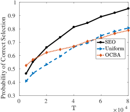
(a) $K=16$

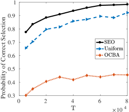
(b) $K=40$

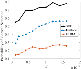
(c) $K=128$

Figure 1: The comparison between SEO, uniform sampling and OCBA in the optimal staffing and pricing problem.

5.2 Optimal dosage in the selection of the best drug

In this example, we consider $K$ different drugs (or treatment plans) that are being compared to treat a disease for a targeted population. Each drug can have different expected effect on the population with different dosage amount (Erman et al. (2006), Verweij et al. (2020)). It is a prior not known for each drug what is the dosage amount that has the best expected effect for that drug among a continuous range of allowable dosage amount. Suppose that one can sequentially do $T$ experiments, where each experiment selects one of the $K$ drugs and a specific dosage of that drug. Suppose that for each experiment, a noisy observation can be obtained on the effect without much delay. The goal is to select one drug with the best expected effect under the best dosage amount for each drug. In this experiment setting, we presume that for each drug, the expected effect as a function of the dosage amount is concave. This concavity assumption on one hand has been captured by empirical evidence for some drugs (e.g., Verweij et al. (2020) identifies a quadratic function form) and on the other hand captures the intuition that neither too small dosage nor too large dosage is desirable.

In the new experiments, we based on the results in Verweij et al. (2020), which examined the dose-response of aprocitentan. The effect is measured by the mean change from baseline in sitting diastolic blood pressure (SiSBP) and the dosage amount ranges from 0 to 50 mg. The small SiSBP is, the better. Since the data is not public, we fit Verweij et al. (2020, Figure 3A) as a quadratic function $a_{*}q^{2}+b_{*}q+c_{*}$ with $a_{*}=9/1250,b_{*}=-23/50,c_{*}=-5$ which is also plotted in Figure 2. We call it the “center” system.

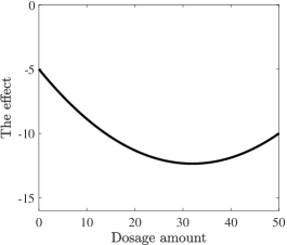
Figure 2: The effect curve with respect to the dosage amount (Verweij et al. 2020, Figure 3A)

We perturb the “center” system to generate $K$ possible systems. Specifically, we first generate $K$ uniform random numbers $u_{1},u_{2},\ldots,u_{K}$ supported in $[-0.1,0.1]$. Then, the $i$-th system is a quadratic function of the form $a_{i}q^{2}+b_{i}q+c_{i}+\epsilon$ with $[a_{i},b_{i},c_{i}]=(1+u_{i})\times[a_{*},b_{*},c_{*}]$ and $\epsilon\sim\mathcal{N}(0,1)$ for $i=1,2,\ldots,K$. For our algorithm (SEO) and the uniform sampling algorithm, we pick the starting point $x_{0}=25$ and the step-size constant $\gamma_{0}=1$. Similar with the simulation optimization discussed in Section 1, we use finite difference gradient estimator with $\Delta_{x}=0.5$. The difference is that we cannot use common random number to generate two samples with $x$ and $x-\Delta_{x}$. Therefore the variance of the gradient will be enlarged. For the OCBA algorithm, we discretize the dosage space as $[11,12,\ldots,40]$.

Figure 3 shows the comparison between SEO, uniform sampling and OCBA algorithms in the optimal dosage problem, which is an analog of 1 in Section 1. We see a clear advantage of our algorithm over the other two algorithms. Since the problem is inherently hard problem as we enforce different drugs have similar effects, the probability of correct selection is still high when $K\leq 40$. More plots are contained in Appendix B.2.

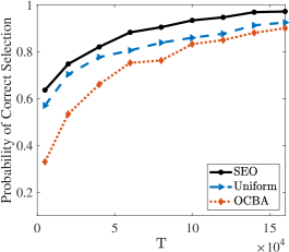
(a) $K=16$

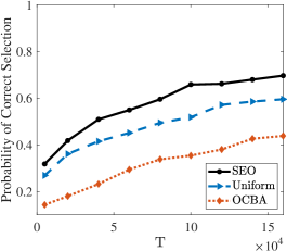
(b) $K=40$

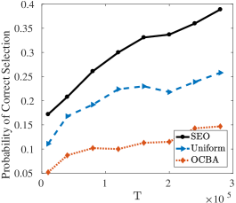
(c) $K=128$

Figure 3: The comparison between SEO, uniform sampling and OCBA in the optimal dosage problem.

5.3 Newsvendor Problem in the selection of the best product

Newsvendor problems Petruzzi and Dada (1999), Arrow et al. (1951), Chen et al. (2016) prevail for decades in revenue management, operations research, and management science, as they are tractable yet still can capture many important realistic characteristics in practice. In the big-data era, date-driven newsvendor problems (Bertsimas and Thiele 2005, Levi et al. 2015, Huber et al. 2019, Ban and Rudin 2019) gains even more attentions since we can utilize more data to get better estimation of uncertainties, therefore informing better business decisions. However, data collection (or data purchasing) can be costly in practice, yielding a need to intelligently collecting data to achieve high-quality decisions.

In this example, we assume there are $K$ products as contenders. Each product is a system, having their own price, cost structure and different demand function. Specifically, we consider the function classes

$$\mathcal{F}_{p,c}=\left\{f_{q}|f_{q}(x)=cq-p\min\left\{q,x\right\},q\geq 0\right\},$$

where $p$ is the price and $c$ denotes the cost. We consider the newsvendar problem

$$v_{i}=\sup_{g\in\mathcal{F}_{p_{i},c_{i}}}\mathbb{E}_{P^{i}}[g(X)]=\sup_{q\geq 0}\mathbb{E}_{P^{i}}[p\min\left\{q,x\right\}-cq],$$

where $p_{i},c_{i},P_{i}$ stands for the price, cost and the demand distribution for the $i$-th product. Here, we assume $p_{i}$ and $c_{i}$ are known beforehand. However $P_{i}$ is not known and we have access to collect costly samples from the distribution $P_{i}$. The goal is to find the best product that gives us the most profits $\max_{i\in\{1,2,\ldots,K\}}$.

For the experiment specifics, we assume that $p_{i}=\tfrac{1}{2}i+5$ and $c_{i}=\tfrac{1}{5}i+1$ and the $P_{i}$ follows $\mathrm{Poi}(\lambda_{i})$, a Poisson distribution with rate $\lambda_{i}=250-6\times i$. The problem (9) can be solved in closed-form since the empirical optimal solution is the $(p_{i}-c_{i})/p_{i}$ quantile of the empirical distribution.

Figure 4 shows the comparison between SEO and uniform sampling algorithms in the newsvendor problem. It is clear that our algorithm has consistently higher probability of correct selection than one of the uniform sampling algorithm. Further, superiority is even more significant when the number of product $K$ is large. We do not compare our algorithm with OCBA since the focus here is the sample-efficiency. Once we collect samples that reflect the unknown underlying distributions, the optimization part is easy and straightforward. Therefore, it is not relevant to discretize the decision space inside each system and perform OCBA. Appendix B.3 contain additional plots.

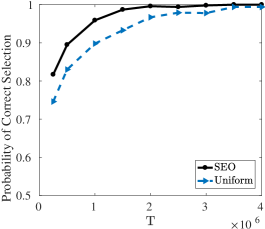
(a) $K=16$

(b) $K=40$

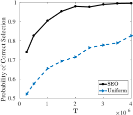
(c) $K=128$

Figure 4: The comparison between SEO and uniform sampling in the newsvendor problem.

6 Conclusion

In this work, we have formulated and provided solutions for a class of problems that we refer to as selecting the best optimizing system (SBOS). In a SBOS problem, there are a finite number of systems as contenders. Inside each system, there is a decision variable that affects the system’s expected performance. The comparison between different systems is based on their expected performances under their own optimally chosen decisions. Without knowing the systems’ expected performances nor what is the optimizing decision inside each system, we design an easy-to-implement algorithm that sequentially assigns samples to different systems and recommends a selection of the best after exhausting a user-specified sampling budget. The proposed algorithm integrates sequential elimination and stochastic gradient descent to exploit the structure inside each system and make comparisons across systems. In this fixed-budget setting, we prove an exponential rate of converge to zero for the algorithm’s probability of false selection as the sampling budget increases. We then demonstrate reliable algorithm performance through three numerical examples.

In future work, we find two lines that are interesting and relevant. The first line concerns a different fixed-precision (or fixed-confidence) framework for SBOS problems, which will have distinct needs for algorithm design and analysis compared to the fixed-budget setting in this work. The second line concerns a distributionally robust framework of SBOS problems. One motivation to consider a distributionally robust setting is because of system non-stationarities, where the probability models built to reflect today’s system can be different (but closely connected) to those of the system in one month. That said, the robust SBOS problems will present a max-max-min structure, demanding new algorithm design and analysis.

Appendix A Proofs of Statements

Appendix A.1 Proof of results in Section 3.2

Proof.

Proof of Proposition 1 Note that

$$\left|\hat{v}_{i}^{T}-v_{i}\right| = \left|\hat{v}_{i}^{T}-\frac{1}{T}\sum_{t=1}^{T}f_{i}(x_{t})+\frac{1}{T}\sum_{t=1}^{T}f_{i}(x_{t})-v_{i}\right|\leq\underbrace{\left|\hat{v}_{i}^{T}-\frac{1}{T}\sum_{t=1}^{T}f_{i}(x_{t})\right|}_{(a)}+\underbrace{\frac{1}{T}v_{i}-\sum_{t=1}^{T}f_{i}(x_{t})}_{(b)}.$$

For part(a), we define a martingale $\{Z_{n}\}_{n=1}^{T}$ with $Z_{0}=0$ and

$$Z_{n}=Z_{n-1}+F_{i}(x_{t},\xi_{t})-\mathbb{E}[F_{i}(x_{t},\xi_{t})|\xi_{1:i-1}]=Z_{n-1}+F_{i}(x_{t},\xi_{t})-f_{i}(x_{t}).$$

We have

$$\exp(\lambda\left(Z_{n}-Z_{n-1}\right)|\xi_{1:i-1})\leq\exp\left(\frac{\lambda^{2}\sigma_{F,i}^{2}}{2}\right).$$

Then, by Azuma’s inequality, we have

$$\mathbb{P}\left(\underbrace{\left|\hat{v}_{i}^{T}-\frac{1}{T}\sum_{t=1}^{T}f_{i}(x_{t})\right|}\geq\epsilon\right)=\mathbb{P}\left(\left|\frac{Z_{T}}{T}\right|\geq\epsilon_{1}\right)\leq 2\exp\left(-\frac{2T\epsilon_{1}^{2}}{\sigma_{F,i}^{2}}\right).$$

For part (b), note that (4.1.10) in Lan (2020) is also vaild for $\frac{1}{T}\sum_{t=1}^{T}f_{i}(x_{t})$ in the sense that

$$v_{i}-\frac{1}{T}\sum_{t=1}^{T}f_{i}(x_{t})\leq\frac{1}{T}\left[\frac{1}{2}\left(x_{1}-x^{\ast}\right)^{2}-\frac{1}{2}\left(x_{T+1}-x^{\ast}\right)^{2}\right.$$

$$+\left.2\sum_{t=1}^{T}\gamma^{2}(M^{2}+\left\|G_{i}(x_{t},\xi_{t})-f_{i}^{\prime}(x_{t})\right\|_{2}^{2}-\sum_{t=1}^{T}\gamma\left\langle G_{i}(x_{t},\xi_{t})-f_{i}^{\prime}(x_{t}),x_{t}-x^{*}\right\rangle\right].$$

And Let $\delta_{t}=G_{i}(x_{t},\xi_{t})-f_{i}^{\prime}(x_{t}).$ Since the step-size is constant, after applying Markov inequality and Assumption 1.3, the (4.1.18) in Lan (2020) can be rewritten as

$$\mathbb{P}\left\{\sum_{t=1}^{T}\left\|\delta_{t}\right\|_{2}^{2}/\sigma_{G,i}^{2}>(1+\lambda)T\right\} \leq \exp(-(1+\lambda)T)\mathbb{E}\left[\exp\left(\sum_{t=1}^{T}\left\|\delta_{t}\right\|_{2}^{2}/\sigma_{G,i}^{2}\right)\right]$$

$$\leq \exp\left(-\lambda T\right).$$

Then, by similar lines with Lan (2020, Proposition 4.1), we have

$$\mathbb{P}\left(v_{i}-\frac{1}{T}\sum_{t=1}^{T}f_{i}(x_{t})\geq\frac{3D_{\mathcal{X}}\sqrt{M^{2}+\sigma^{2}}}{\sqrt{T}}+\epsilon_{2}\right)\leq\exp(-\epsilon_{2}T\sqrt{T}/\left(3\sigma_{G,i}D_{\mathcal{X}_{i}}\right))+\exp\left(-\epsilon_{2}^{2}T/\left(27\sigma_{G,i}^{2}D_{\mathcal{X}}^{2}\right)\right).$$

We let $\epsilon_{1}=\frac{\left(\sigma_{F,i}/\sqrt{2}\right)\epsilon}{3\sqrt{3}\sigma_{G,i}D_{\mathcal{X}_{i}}+\sigma_{F,i}/\sqrt{2}}$ and $\epsilon_{2}=\frac{3\sqrt{3}\sigma_{G,i}D_{\mathcal{X}_{i}}\epsilon}{3\sqrt{3}\sigma_{G,i}D_{\mathcal{X}_{i}}+\sigma_{F,i}/\sqrt{2}}.$ Then, we have

$$\frac{\epsilon_{2}^{2}}{27\sigma_{G,i}^{2}D_{\mathcal{X}_{i}}^{2}}=\frac{2\epsilon_{1}^{2}}{\sigma_{F,i}^{2}}=\frac{\epsilon^{2}}{\left(3\sqrt{3}\sigma_{G,i}D_{\mathcal{X}_{i}}+\sigma_{F,i}/\sqrt{2}\right)^{2}}.$$

∎

Proof of Theorem 1.

We rely on the proof of Theorem 33.10 in Lattimore and Szepesvári (2020). It is easy to note that $|\mathcal{A}_{\ell}|=\lfloor K2^{1-\ell}\rfloor$ and $T_{\ell}\geq T2^{\ell-1}/\lfloor\log_{2}\left(K\right)\rfloor/K.$ We first observe that

$$\mathbb{P}(\hat{v}_{1}^{T_{\ell}}\leq\hat{v}_{i}^{T_{\ell}}|\left\{i,1\right\}\subset\mathcal{A}_{\ell})\leq\mathbb{P}\left(\hat{v}_{1}^{T_{\ell}}\leq v_{1}+\Delta_{i}/2\right)+\mathbb{P}\left(\hat{v}_{i}^{T_{\ell}}\geq v_{i}-\Delta_{i}/2\right).$$

Since $T\geq\lfloor\log_{2}\left(K\right)\rfloor K\left(\max_{i\in[K]}\frac{24D_{\mathcal{X}_{i}}}{\Delta_{i}}\left(\sqrt{M^{2}+\sigma_{G,i}^{2}}\right)\right)^{2}$, we have

$$\frac{3D_{\mathcal{X}_{i}}\sqrt{M^{2}+\sigma_{G,i}^{2}}}{\sqrt{T_{l}}}\leq\Delta_{i}/4.$$

By letting $\epsilon=\Delta_{i}/4,$ and applying Proposition 1 we have

$$\mathbb{P}\left(\left|\hat{v}_{i}^{T_{\ell}}-v_{i}\right|\geq\Delta_{i}/4\right)\leq 3\exp\left(-\frac{T_{\ell}\epsilon^{2}}{16\left(3\sqrt{3}\sigma_{G,i}D_{\mathcal{X}_{i}}+\sigma_{F,i}/\sqrt{2}\right)^{2}}\right)+\exp\left(-\frac{\Delta_{i}T_{\ell}\sqrt{T_{\ell}}}{4(3\sigma_{G,i}D_{\mathcal{X}_{i}}+\sigma_{F,i}/\sqrt{6})}\right),$$

which in turn gives us

$$\mathbb{P}(\hat{v}_{1}^{T_{\ell}}\leq\hat{v}_{i}^{T_{\ell}}|\left\{i,1\right\}\subset\mathcal{A}_{\ell})\leq 6\exp\left(-\frac{T_{\ell}\Delta_{i}^{2}}{48M_{\sigma}^{2}}\right)+2\exp\left(-\frac{\Delta_{i}T_{\ell}\sqrt{T_{\ell}}}{4M_{\sigma}}\right).$$ (A.2)

Next, we define a new set

$$\mathcal{A}_{\ell}^{\prime}=\left\{i\in\mathcal{A}_{\ell}\left|\sum_{j\leq i}\mathbb{I}\left\{j\in A\right\}>\lfloor\left|\mathcal{A}_{\ell}\right|/4\rfloor\right.\right\},$$

to be the bottom (ordered by true value) three-quarters of the systems in round $\ell.$ Then, if the optimal system is eliminated in this round, we must have

$$N_{\ell}=\sum_{i\in\mathcal{A}_{\ell}^{\prime}}\mathbb{I}\{\hat{v}_{1}^{\ell}\geq\hat{v}_{i}^{\ell}\}\geq\left\lfloor\frac{1}{3}(|\mathcal{A}_{\ell}^{\prime}|+1)\right\rfloor.$$ (A.3)

On the other hand, by applying the union bound to the bound (A.2),

$$\mathbb{E}\left[N_{\ell}\right]\leq|\mathcal{A}_{\ell}^{\prime}|\max_{i\in\mathcal{A}_{\ell}^{\prime}}\left\{6\exp\left(-\frac{T_{\ell}\Delta_{i}^{2}}{48M^{2}}\right)+2\exp\left(-\frac{\Delta_{i}T_{\ell}\sqrt{T_{\ell}}}{4M}\right)\right\}.$$

Let $i_{\ell}^{\prime}\triangleq\min\mathcal{A}_{\ell}^{\prime}$ $\geq\lfloor\left|\mathcal{A}_{\ell}\right|/4\rfloor+1\geq K2^{-1-\ell}.$ Then, we have

$$\mathbb{E}\left[N_{\ell}\right] \leq|\mathcal{A}_{\ell}^{\prime}|\max_{i\in\mathcal{A}_{\ell}^{\prime}}\left\{6\exp\left(-\frac{2^{\ell+1}T\Delta_{i}^{2}}{192K\lfloor\log_{2}(K)\rfloor M_{\sigma}^{2}}\right)+2\exp\left(-\frac{\Delta_{i}2^{\ell+1}T\sqrt{T2^{\ell-1}/\lfloor\log_{2}(K)\rfloor/K}}{16K\lfloor\log_{2}(K)\rfloor M_{\sigma}}\right)\right\}$$ (A.4)

$$\leq|\mathcal{A}_{\ell}^{\prime}|\max_{i\in\mathcal{A}_{\ell}^{\prime}}\left\{6\exp\left(-\frac{T\Delta_{i_{\ell}^{\prime}}^{2}}{192\lfloor\log_{2}(K)\rfloor M_{\sigma}^{2}i_{\ell}^{\prime}}\right)+2\exp\left(-\frac{T\sqrt{T}\Delta_{i_{\ell}^{\prime}}}{16\sqrt{K\lfloor\log_{2}(K)\rfloor^{2}}M_{\sigma}i_{\ell}^{\prime}}\right)\right\}.$$ (A.5)

By combining (A.3) and (A.5), we have

$$\mathbb{P}(1\notin\mathcal{A}_{\ell+1}|1\in\mathcal{A}_{\ell}) \leq\mathbb{P}\left(N_{\ell}\geq\left\lfloor\frac{1}{3}(|\mathcal{A}_{\ell}^{\prime}|+1)\right\rfloor\right)\leq\frac{\mathbb{E}[N_{\ell}]}{\left\lfloor(|\mathcal{A}_{\ell}^{\prime}|+1)/3\right\rfloor}$$

$$\leq 4\max_{i\in\mathcal{A}_{\ell}^{\prime}}\left\{6\exp\left(-\frac{T\Delta_{i_{\ell}^{\prime}}^{2}}{192\lfloor\log_{2}(K)\rfloor M_{\sigma}^{2}i_{\ell}^{\prime}}\right)+2\exp\left(-\frac{T\sqrt{T}\Delta_{i_{\ell}^{\prime}}}{16\sqrt{K\lfloor\log_{2}(K)\rfloor^{2}}M_{\sigma}i_{\ell}^{\prime}}\right)\right\}.$$

Finally, by adding the above inequality for all $\ell$ from $1$ to L, we have

$$\mathbb{P}(1 \notin \mathcal{A}_{L+1})\leq\sum_{\ell=1}^{L}\mathbb{P}(1\notin\mathcal{A}_{\ell+1}|1\in\mathcal{A}_{\ell})$$

$$\leq \lfloor\log_{2}(K)\rfloor\left\{24\exp\left(-\frac{T}{192\lfloor\log_{2}(K)\rfloor M_{\sigma}^{2}H_{2}(v)}\right)+8\exp\left(-\frac{T\sqrt{T}}{16\sqrt{K\lfloor\log_{2}(K)\rfloor^{2}}M_{\sigma}H^{\prime}_{2}(v)}\right)\right\},$$

where $H_{2}(v)=\max_{i>1}\frac{i}{\Delta_{i}^{2}},$ and $H^{\prime}_{2}(v)=\max_{i>1}\frac{i}{\Delta_{i}}$.

$\square$ ∎

Appendix A.2 Proof of results in Section 2

We first collect some useful results.

Definition 3 (Rademacher complexity).

Let $\mathcal{F}$ be a family of real-valued functions $f:Z\rightarrow\mathbb{R}$ Then, the Rademacher complexity of $\mathcal{F}$ is defined as

$$\mathcal{R}_{n}\left(\mathcal{F}\right)\triangleq\mathbb{E}_{z,\sigma}\left[\sup_{f\in\mathcal{F}}\left|\frac{1}{n}\sum_{i=1}^{n}\sigma_{i}f(z_{i})\right|\right],$$

where $\sigma_{1},\sigma_{2},\ldots,\sigma_{n}$ are i.i.d with the distribution $\mathbb{P}\left(\sigma_{i}=1\right)=\mathbb{P}\left(\sigma_{i}=-1\right)=1/2.$

Theorem A3 (Theorem 4.10 in Wainwright (2019)).

If $f(z)\in[-B,B],$ we have with probability at least $1-\exp\left(-\frac{n\epsilon^{2}}{2B^{2}}\right)$,

$$\sup_{f\in\mathcal{F}}\left|\frac{1}{n}\sum_{i=1}^{n}f(z_{i})-\mathbb{E}f(z)\right|\leq 2\mathcal{R}_{n}\left(\mathcal{F}\right)+\epsilon.$$

Theorem A4 (Dudley’s Theorem, (5.48) in Wainwright (2019)).

If $f(z)\in[-B,B],$ we have a bound for the Rademacher complexity,

$$\mathcal{R}_{n}\left(\mathcal{F}\right)\leq\frac{24\mathcal{J}(\mathcal{F},P)}{\sqrt{n}},$$

where $N(t,\mathcal{F}$,$\left\|\cdot\right\|_{P_{n}})$ is $t$-covering number of set $\mathcal{F}$ and

Proof of Theorem 2.

Let $g_{\ast}^{i}=\arg\max_{g\in\mathcal{F}_{i}}\mathbb{E}_{P^{i}}\left[g(X)\right].$ Then,

$$v_{i}-\hat{v}_{i}^{n_{i}} = \mathbb{E}_{P^{i}}\left[g_{*}^{i}(X)\right]-\mathbb{E}_{P_{n_{i}}^{i}}\left[g_{\ast}^{i}(X)\right]+\mathbb{E}_{P_{n_{i}}^{i}}\left[g_{\ast}^{i}(X)\right]-\sup_{g\in\mathcal{F}_{i}}\mathbb{E}_{P_{n_{i}}^{i}}\left[g(X)\right]$$

$$\leq \sup_{g\in\mathcal{F}_{i}}\left|\mathbb{E}_{P_{n_{i}}^{i}}\left[g(X)\right]-\mathbb{E}_{P^{i}}\left[g(X)\right]\right|.$$

Similarly, we have

$$\hat{v}_{i}^{n_{i}}-v_{i}\leq\sup_{g\in\mathcal{F}_{i}}\left|\mathbb{E}_{P_{n_{i}}^{i}}\left[g(X)\right]-\mathbb{E}_{P^{i}}\left[g(X)\right]\right|.$$

We define $\mathcal{R}_{n}$ as the Rademacher complexity (Definition 3). By Theorems A3 and A4, we have with probability at least $1-\exp\left(-\frac{n_{i}\epsilon^{2}}{2B^{2}}\right)$,

$$\left|v_{i}-\hat{v}_{i}^{n_{i}}\right|\leq\sup_{f\in\mathcal{F}_{i}}\left|\frac{1}{n_{i}}\sum_{i=1}^{n_{i}}g(z_{i})-\mathbb{E}g(z)\right|\leq 2\mathcal{R}_{n_{i}}\left(\mathcal{F}_{i}\right)+\epsilon\leq\frac{48\mathcal{J}(\mathcal{F},P)}{\sqrt{n_{i}}}+\epsilon,$$

which means

$$\mathbb{P}\left(\hat{v}_{i}^{n_{i}}\notin\left(v_{i}-\frac{48\mathcal{J}(\mathcal{F},P)}{\sqrt{n_{i}}}-\epsilon,v_{i}+\frac{48\mathcal{J}(\mathcal{F},P)}{\sqrt{n_{i}}}+\epsilon\right)\right)\leq\exp\left(-\frac{n_{i}\epsilon^{2}}{2B^{2}}\right).$$

Note that $|\mathcal{A}_{\ell}|=\lfloor K2^{1-\ell}\rfloor$ and $T_{\ell}\geq T2^{\ell-1}/\lfloor\log_{2}\left(K\right)\rfloor/K.$ Similar with the proof of Theorem 1, we observe

$$\mathbb{P}(\hat{v}_{1}^{T_{\ell}}\leq\hat{v}_{i}^{T_{\ell}}|\left\{i,1\right\}\subset\mathcal{A}_{\ell})\leq\mathbb{P}\left(\hat{v}_{1}^{T_{\ell}}\leq v_{1}+\Delta_{i}/2\right)+\mathbb{P}\left(\hat{v}_{i}^{T_{\ell}}\geq v_{i}-\Delta_{i}/2\right).$$

Since $T\geq\lfloor\log_{2}\left(K\right)\rfloor K\left(\max_{i\in[K]}\frac{192}{\Delta_{i}}\left(\mathcal{J}(\mathcal{F}_{i},P^{i})\right)\right)^{2},$ we have

$$\frac{48\mathcal{J}(\mathcal{F},P)}{\sqrt{n_{i}}}\leq\Delta_{i}/4.$$

By letting $\epsilon=\Delta_{i}/4,$ we have

$$\mathbb{P}(\hat{v}_{1}^{T_{\ell}}\geq\hat{v}_{i}^{\ell}|\left\{i,1\right\}\subset\mathcal{A}_{\ell})\leq 2\exp\left(-\frac{T_{\ell}\Delta_{i}^{2}}{32B^{2}}\right).$$ (A.6)

Next, we define a new set

$$\mathcal{A}_{\ell}^{\prime}=\left\{i\in\mathcal{A}_{\ell}\left|\sum_{j\leq i}\mathbb{I}\left\{j\in A\right\}>\lfloor\left|\mathcal{A}_{\ell}\right|/4\rfloor\right.\right\},$$

to be the bottom (ordered by true value) three-quarters of the systems in round $\ell.$ Then, if the optimal system is eliminated in this round, we must have

$$N_{\ell}=\sum_{i\in\mathcal{A}_{\ell}^{\prime}}\mathbb{I}\{\hat{v}_{1}^{\ell}\geq\hat{v}_{i}^{\ell}\}\geq\left\lfloor\frac{1}{3}(|\mathcal{A}_{\ell}^{\prime}|+1)\right\rfloor.$$ (A.7)

On the other hand, by applying the union bound to the bound (A.6),

$$\mathbb{E}\left[N_{\ell}\right]\leq 2|\mathcal{A}_{\ell}^{\prime}|\max_{i\in\mathcal{A}_{\ell}^{\prime}}\exp\left(-\frac{T2^{\ell-1}\Delta_{i}^{2}}{32B^{2}K}\right).$$

Let $i_{\ell}^{\prime}\triangleq\min\mathcal{A}_{\ell}^{\prime}$ $\geq\lfloor\left|\mathcal{A}_{\ell}\right|/4\rfloor+1\geq K2^{-1-\ell}.$ Then, we have

$$\mathbb{E}\left[N_{\ell}\right]\leq 2|\mathcal{A}_{\ell}^{\prime}|\max_{i\in\mathcal{A}_{\ell}^{\prime}}\exp\left(-\frac{T2^{\ell+1}\Delta_{i}^{2}}{128B^{2}\lfloor\log_{2}\left(K\right)\rfloor K}\right)\leq 2|\mathcal{A}_{\ell}^{\prime}|\exp\left(-\frac{T\Delta_{i_{\ell}^{\prime}}^{2}}{128B^{2}\lfloor\log_{2}\left(K\right)\rfloor i_{\ell}^{\prime}}\right).$$ (A.8)

By combining (A.7) and (A.8), we have

$$\mathbb{P}(1\notin\mathcal{A}_{\ell+1}|1\in\mathcal{A}_{\ell})\leq\mathbb{P}\left(N_{\ell}\geq\frac{1}{3}|\mathcal{A}_{\ell}^{\prime}|\right)\leq 8\exp\left(-\frac{T\Delta_{i_{\ell}^{\prime}}^{2}}{128B^{2}\lfloor\log_{2}\left(K\right)\rfloor i_{\ell}^{\prime}}\right).$$

Finally, by adding the above inequality for all $\ell$ from $1$ to L, we have

$$\mathbb{P}(1\notin\mathcal{A}_{L+1})\leq\sum_{\ell=1}^{L}\mathbb{P}(1\notin\mathcal{A}_{\ell+1}|1\in\mathcal{A}_{\ell})\leq 8\lfloor\log_{2}(K)\rfloor\exp\left(-\frac{N}{128B^{2}\lfloor\log_{2}\left(K\right)\rfloor H_{2}(G)}\right),$$

where $H_{2}(G)=\max_{i>1}\frac{i}{\Delta_{i}^{2}}.$

$\square$ ∎

Appendix A.3 Proof of results in Section 5

Proof of Lemma 1.

: We consider $\mathcal{X}\subset\mathbb{R}$. Without loss of generality, we assume $x_{1}<x_{2}<\ldots<x_{d}$. By the pigeonhole principle, there exists a pair of adjacent discretization points whose distance is no less than $D_{\mathcal{X}}/(d+1)$ Then, we assume $x_{j+1}-x_{j}\geq D_{\mathcal{X}}/(d+1)$ Then, we construct $K$ systems, where the first and the second systems are identical on the region $((-\infty,x_{j}]\cup[x_{j+1},+\infty))\cap\mathcal{X}$. Therefore, for $x\in((-\infty,x_{j}]\cup[x_{j+1},+\infty))\cap\mathcal{X}$, we assume

$$F_{i}(x,\xi)=-M|x-(x_{j}+x_{j+1})/2|+\xi,\text{ for }i=1,2,$$

where $\xi$ is a common random variable with mean zero and variance $\sigma_{F}^{2}$. And for $x\in(x_{j-1},x_{j})$, we assume

$$F_{1}(x,\xi)=-M|x-(x_{j}+x_{j+1})/2|+\xi\text{ and }F_{2}(x,\xi)=-M|(x_{j}-x_{j+1})/2|.$$

In this construction, $F_{1}$ $F_{2}$ are concave. $v_{3},v_{4},\ldots,v_{K}$ could be arbitrary small such that for any $\varepsilon>0$, the complexity

$$H<(M|(x_{j}-x_{j+1})/2|)^{-2}+\varepsilon\leq\frac{1}{(MD_{\mathcal{X}}/(d+1)/2)^{2}}+\varepsilon.$$

If $d+1<\frac{MD_{\mathcal{X}}\sqrt{a}}{2}$, we have $H\leq a$ by taking $\varepsilon$ sufficiently small, which means the constructed instance is in $\mathcal{O}_{M,\mathcal{X},K,a}$. Since the first and the second systems are identical at the discretization set, it is impossible for Algorithm 5 to correctly select the best system. ∎

Appendix B Numerical Results

In this section, we provide additional plots regarding different $K$’s.

Appendix B.1 Optimal staffing and pricing in queueing simulation optimization

(a) $K=16$

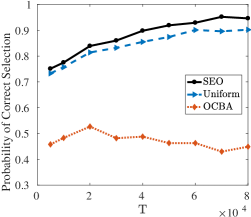
(b) $K=24$

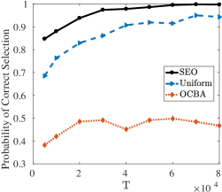
(c) $K=32$

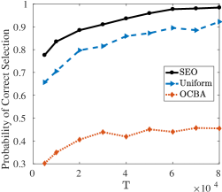
(d) $K=40$

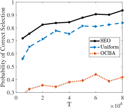
(e) $K=48$

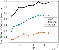
(f) $K=128$

Figure 5: The comparison between SEO, uniform sampling and OCBA in the optimal staffing and pricing problem.

Appendix B.2 Optimal Dosage in the selection of the best drug

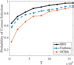
(a) $K=16$

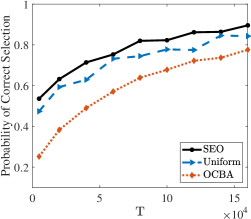
(b) $K=24$

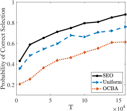
(c) $K=32$

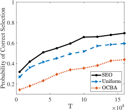
(d) $K=40$

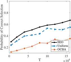
(e) $K=48$

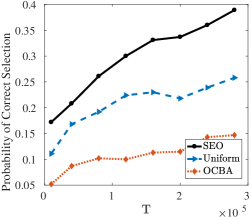
(f) $K=128$

Figure 6: The comparison between SEO, uniform sampling and OCBA in the optimal dosage problem.

Appendix B.3 Newsvendor Problem in the selection of the best product

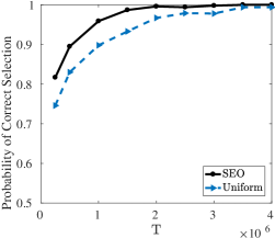
(a) $K=16$

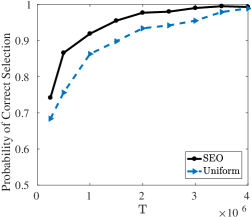
(b) $K=24$

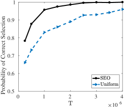
(c) $K=32$

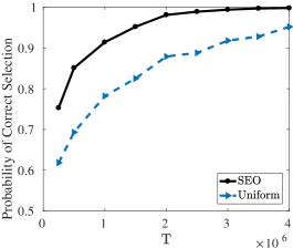
(d) $K=40$

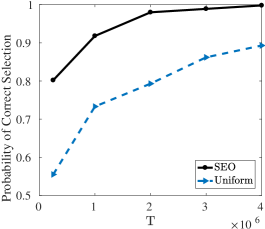
(e) $K=64$

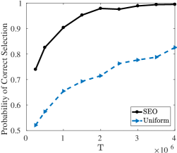
(f) $K=128$

Figure 7: The comparison between SEO and uniform sampling in the newsvendor problem.

References

- Agarwal et al. (2009) Alekh Agarwal, Martin J Wainwright, Peter Bartlett, and Pradeep Ravikumar. Information-theoretic lower bounds on the oracle complexity of convex optimization. Advances in Neural Information Processing Systems, 22:1–9, 2009.
- Arrow et al. (1951) Kenneth J Arrow, Theodore Harris, and Jacob Marschak. Optimal inventory policy. Econometrica: Journal of the Econometric Society, pages 250–272, 1951.
- Audibert et al. (2010) Jean-Yves Audibert, Sébastien Bubeck, and Rémi Munos. Best arm identification in multi-armed bandits. In COLT, pages 41–53. Citeseer, 2010.
- Ban and Rudin (2019) Gah-Yi Ban and Cynthia Rudin. The big data newsvendor: Practical insights from machine learning. Operations Research, 67(1):90–108, 2019.
- Bechhofer et al. (1995) RE Bechhofer, TJ Santner, and DM Goldsman. Design and analysis of experiments for statistical selection, screening, and multiple comparison john wiley and sons. Hoboken, New Jersey, 1995.
- Bechhofer (1954) Robert E Bechhofer. A single-sample multiple decision procedure for ranking means of normal populations with known variances. The Annals of Mathematical Statistics, pages 16–39, 1954.
- Bertsimas and Thiele (2005) Dimitris Bertsimas and Aurélie Thiele. A data-driven approach to newsvendor problems. Working Papere, Massachusetts Institute of Technology, 2005.
- Carpentier and Locatelli (2016) Alexandra Carpentier and Andrea Locatelli. Tight (lower) bounds for the fixed budget best arm identification bandit problem. In Conference on Learning Theory, pages 590–604. PMLR, 2016.
- Chen et al. (2000) Chun-Hung Chen, Jianwu Lin, Enver Yücesan, and Stephen E Chick. Simulation budget allocation for further enhancing the efficiency of ordinal optimization. Discrete Event Dynamic Systems, 10(3):251–270, 2000.
- Chen et al. (2016) Rachel R Chen, TCE Cheng, Tsan-Ming Choi, Yulan Wang, et al. Novel advances in applications of the newsvendor model. 2016.
- Chen et al. (2020) Xinyun Chen, Yunan Liu, and Guiyu Hong. An online learning approach to dynamic pricing and capacity sizing in service systems. arXiv preprint arXiv:2009.02911, 2020.
- Chen and Ryzhov (2019) Ye Chen and Ilya O Ryzhov. Complete expected improvement converges to an optimal budget allocation. Advances in Applied Probability, 51(1):209–235, 2019.
- Chick (2006) Stephen E Chick. Subjective probability and bayesian methodology. Handbooks in Operations Research and Management Science, 13:225–257, 2006.
- Chick and Frazier (2012) Stephen E Chick and Peter Frazier. Sequential sampling with economics of selection procedures. Management Science, 58(3):550–569, 2012.
- Chick and Wu (2005) Stephen E Chick and Yaozhong Wu. Selection procedures with frequentist expected opportunity cost bounds. Operations Research, 53(5):867–878, 2005.
- Chick et al. (2010) Stephen E Chick, Jürgen Branke, and Christian Schmidt. Sequential sampling to myopically maximize the expected value of information. INFORMS Journal on Computing, 22(1):71–80, 2010.
- Chick et al. (2021) Stephen E Chick, Noah Gans, and Özge Yapar. Bayesian sequential learning for clinical trials of multiple correlated medical interventions. Management Science, 2021.
- Erman et al. (2006) Milton Erman, David Seiden, Gary Zammit, Stephen Sainati, and Jeffrey Zhang. An efficacy, safety, and dose–response study of ramelteon in patients with chronic primary insomnia. Sleep medicine, 7(1):17–24, 2006.
- Fan et al. (2016) Weiwei Fan, L Jeff Hong, and Barry L Nelson. Indifference-zone-free selection of the best. Operations Research, 64(6):1499–1514, 2016.
- Fan et al. (2020) Weiwei Fan, L Jeff Hong, and Xiaowei Zhang. Distributionally robust selection of the best. Management Science, 66(1):190–208, 2020.
- Frazier et al. (2009) Peter Frazier, Warren Powell, and Savas Dayanik. The knowledge-gradient policy for correlated normal beliefs. INFORMS journal on Computing, 21(4):599–613, 2009.
- Frazier (2014) Peter I Frazier. A fully sequential elimination procedure for indifference-zone ranking and selection with tight bounds on probability of correct selection. Operations Research, 62(4):926–942, 2014.
- Gabillon et al. (2011) Victor Gabillon, Mohammad Ghavamzadeh, Alessandro Lazaric, and Sébastien Bubeck. Multi-bandit best arm identification. In Proceedings of the 24th International Conference on Neural Information Processing Systems, pages 2222–2230, 2011.
- Glynn and Juneja (2004) Peter Glynn and Sandeep Juneja. A large deviations perspective on ordinal optimization. In Proceedings of the 2004 Winter Simulation Conference, 2004., volume 1. IEEE, 2004.
- Hong and Nelson (2007) L Jeff Hong and Barry L Nelson. Selecting the best system when systems are revealed sequentially. Iie Transactions, 39(7):723–734, 2007.
- Hong et al. (2021) L Jeff Hong, Weiwei Fan, and Jun Luo. Review on ranking and selection: A new perspective. Frontiers of Engineering Management, 8(3):321–343, 2021.
- Huber et al. (2019) Jakob Huber, Sebastian Müller, Moritz Fleischmann, and Heiner Stuckenschmidt. A data-driven newsvendor problem: From data to decision. European Journal of Operational Research, 278(3):904–915, 2019.
- Hunter and Nelson (2017) Susan R Hunter and Barry L Nelson. Parallel ranking and selection. In Advances in Modeling and Simulation, pages 249–275. Springer, 2017.
- Johari et al. (2021) Ramesh Johari, Pete Koomen, Leonid Pekelis, and David Walsh. Always valid inference: Continuous monitoring of a/b tests. Operations Research, 2021.
- Kim and Randhawa (2018) Jeunghyun Kim and Ramandeep S Randhawa. The value of dynamic pricing in large queueing systems. Operations Research, 66(2):409–425, 2018.
- Kim and Nelson (2006) Seong-Hee Kim and Barry L Nelson. Selecting the best system. Handbooks in operations research and management science, 13:501–534, 2006.
- Lan (2020) Guanghui Lan. First-order and Stochastic Optimization Methods for Machine Learning. Springer Nature, 2020.
- Lan et al. (2010) Hai Lan, Barry L Nelson, and Jeremy Staum. A confidence interval procedure for expected shortfall risk measurement via two-level simulation. Operations Research, 58(5):1481–1490, 2010.
- Lattimore and Szepesvári (2020) Tor Lattimore and Csaba Szepesvári. Bandit algorithms. Cambridge University Press, 2020.
- Lee and Ward (2014) Chihoon Lee and Amy R Ward. Optimal pricing and capacity sizing for the gi/gi/1 queue. Operations Research Letters, 42(8):527–531, 2014.
- Lee and Ward (2019) Chihoon Lee and Amy R Ward. Pricing and capacity sizing of a service facility: Customer abandonment effects. Production and Operations Management, 28(8):2031–2043, 2019.
- Levi et al. (2015) Retsef Levi, Georgia Perakis, and Joline Uichanco. The data-driven newsvendor problem: new bounds and insights. Operations Research, 63(6):1294–1306, 2015.
- Li et al. (2020) Haidong Li, Henry Lam, Zhe Liang, and Yijie Peng. Context-dependent ranking and selection under a bayesian framework. In 2020 Winter Simulation Conference (WSC), pages 2060–2070. IEEE, 2020.
- Luo et al. (2015) Jun Luo, L Jeff Hong, Barry L Nelson, and Yang Wu. Fully sequential procedures for large-scale ranking-and-selection problems in parallel computing environments. Operations Research, 63(5):1177–1194, 2015.
- Nemirovskij and Yudin (1983) Arkadij Semenovič Nemirovskij and David Borisovich Yudin. Problem complexity and method efficiency in optimization. 1983.
- Petruzzi and Dada (1999) Nicholas C Petruzzi and Maqbool Dada. Pricing and the newsvendor problem: A review with extensions. Operations research, 47(2):183–194, 1999.
- Russo (2020) Daniel Russo. Simple bayesian algorithms for best-arm identification. Operations Research, 68(6):1625–1647, 2020.
- Ryzhov (2016) Ilya O Ryzhov. On the convergence rates of expected improvement methods. Operations Research, 64(6):1515–1528, 2016.
- Shen et al. (2021) Haihui Shen, L Jeff Hong, and Xiaowei Zhang. Ranking and selection with covariates for personalized decision making. INFORMS Journal on Computing, 2021.
- Van der Vaart (2000) Aad W Van der Vaart. Asymptotic statistics, volume 3. Cambridge university press, 2000.
- Vapnik and Chervonenkis (1971) VN Vapnik and A Ya Chervonenkis. On the uniform convergence of relative frequencies of events to their probabilities. Measures of Complexity, 16(2):11, 1971.
- Verweij et al. (2020) Pierre Verweij, Parisa Danaietash, Bruno Flamion, Joël Ménard, and Marc Bellet. Randomized dose-response study of the new dual endothelin receptor antagonist aprocitentan in hypertension. Hypertension, 75(4):956–965, 2020.
- Waeber et al. (2010) Rolf Waeber, Peter I Frazier, and Shane G Henderson. Performance measures for ranking and selection procedures. In Proceedings of the 2010 Winter Simulation Conference, pages 1235–1245. IEEE, 2010.
- Wainwright (2019) Martin J Wainwright. High-dimensional statistics: A non-asymptotic viewpoint, volume 48. Cambridge University Press, 2019.
- Wu and Zhou (2018) Di Wu and Enlu Zhou. Analyzing and provably improving fixed budget ranking and selection algorithms. arXiv preprint arXiv:1811.12183, 2018.