Stability Based Generalization Bounds
for Exponential Family Langevin Dynamics

Abstract

Recent years have seen advances in generalization bounds for noisy stochastic algorithms, especially stochastic gradient Langevin dynamics (SGLD) based on stability (Mou et al.,, 2018; Li et al.,, 2020) and information theoretic approaches (Xu and Raginsky,, 2017; Negrea et al.,, 2019; Steinke and Zakynthinou,, 2020). In this paper, we unify and substantially generalize stability based generalization bounds and make three technical contributions. First, we bound the generalization error in terms of expected (not uniform) stability which arguably leads to quantitatively sharper bounds. Second, as our main contribution, we introduce Exponential Family Langevin Dynamics (EFLD), a substantial generalization of SGLD, which includes noisy versions of Sign-SGD and quantized SGD as special cases. We establish data-dependent expected stability based generalization bounds for any EFLD algorithm with a $O(1/n)$ sample dependence and dependence on gradient discrepancy rather than the norm of gradients, yielding significantly sharper bounds. Third, we establish optimization guarantees for special cases of EFLD. Further, empirical results on benchmarks illustrate that our bounds are non-vacuous, quantitatively sharper than existing bounds, and behave correctly under noisy labels.

1 Introduction

Recent years have seen renewed interest in characterizing generalization performance of learning algorithms in terms of stability which considers change in performance of a learning algorithm based on change of a single training point (Hardt et al.,, 2016; Bousquet and Elisseeff,, 2002; Li et al.,, 2020; Mou et al.,, 2018). For stochastic gradient descent (SGD), Hardt et al., (2016) established generalization bounds based on uniform stability (Bousquet and Elisseeff,, 2002), although the analysis needed rather small step sizes $\eta_{t}=1/t$ which is arguably not useful in practice. While improving the stability analysis for SGD has remained a challenge, advances have been made on noisy SGD algorithms, especially stochastic gradient Langevin dynamics (SGLD) (Welling and Teh,, 2011; Mou et al.,, 2018; Li et al.,, 2020) which adds Gaussian noise to the stochastic gradients. In parallel, there has been key developments on related information-theoretic generalization bounds applicable to SGLD type algorithms (Negrea et al.,, 2019; Haghifam et al.,, 2020; Xu and Raginsky,, 2017; Russo and Zou,, 2016; Pensia et al.,, 2018; Wang et al., 2021b, ).

While these developments have led to advances in analyzing generalization of noisy SGD algorithms, and we elaborate on these developments in Appendix A, they each have certain limitations, e.g., dependence on global Lipschitz constant $L$ (Mou et al.,, 2018), tiny $O(1/L)$ step sizes (Li et al.,, 2020), $O(1/\sqrt{n})$ sample dependence (Mou et al.,, 2018; Negrea et al.,, 2019), dependence on gradient norms (Li et al.,, 2020), restrictions on nature of mini-batching (Wang et al., 2021b, ), etc. Further, most prior work primarily focuses on SGLD and cannot be readily extended to popular variants such as noisy versions of Sign-SGD or quantized SGD (Bernstein et al., 2018a, ; Alistarh et al.,, 2017; Jiang and Agrawal,, 2018). In this paper, we build on the core strengths of such existing approaches, most notably (a) the $O({1}/{n})$ sample dependence of stability based bounds (Mou et al.,, 2018; Li et al.,, 2020), (b) the dependence on some measures of gradient discrepancy rather than the norm of gradients (Negrea et al.,, 2019; Haghifam et al.,, 2020), and (c) no dependence on the global Lipschitz constant $L$, and develop a framework (Section 2) for establishing generalization bounds for a general family of noisy stochastic iterative algorithms which includes SGLD as a special case. Our framework considers generalization based on the concept of expected stability, rather than uniform stability (Hardt et al.,, 2016; Bousquet and Elisseeff,, 2002; Bousquet et al.,, 2020; Mou et al.,, 2018; Farghly and Rebeschini,, 2021), and yields distribution dependent generalization bounds which avoid the worst-case setting of uniform stability. Recall that for any data domain ${\cal Z}$ and a distribution $D$ over the domain, uniform stability considers the worst case difference in loss over two datasets $S_{n},S^{\prime}_{n}\in{\cal Z}^{n}$ of size $n$ which differ by one point, i.e., over $\sup_{S_{n},S^{\prime}_{n},|S_{n}\Delta S^{\prime}_{n}|=1}\cdots$ (Bousquet and Elisseeff,, 2002; Hardt et al.,, 2016). In Section 2, we show that one gets a valid generalization bound for stochastic algorithms by replacing the supremum $\sup$ by an expectation $\mathbb{E}_{S_{n},S^{\prime}_{n}}$, where $S_{n}\sim D^{n}$ and, without loss of generality, $S^{\prime}_{n}$ shares the first $(n-1)$ samples with $S_{n}$ with the $n$-th sample $z^{\prime}_{n}\sim D$. Replacing $\sup$ by $\mathbb{E}$ makes the bound distribution dependent and arguably leads to quantitatively sharper and computable bounds with less assumptions. Further, we show that expected stability of general noisy stochastic iterative algorithms can be bounded by the expectation of a Le Cam Style Divergence (LSD) between distributions over parameters obtained from $S_{n}$ and $S^{\prime}_{n}$. Thus, getting an expected stability based generalization bound for a specific stochastic algorithm reduces to that of bounding the expected LSD.

In Section 3, we introduce Exponential Family Langevin Dynamics (EFLD), a family of noisy stochastic gradient descent algorithms based on exponential family noise. Special cases of EFLD include SGLD and noisy versions of Sign-SGD or quantized SGD algorithms (Bernstein et al., 2018a, ; Bernstein et al., 2018b, ; Jin et al.,, 2020; Alistarh et al.,, 2017). Our main result provides an expected stability based generalization bound for any EFLD algorithm with several aforementioned desirable properties: (a) a $O({1}/{n})$ sample dependence, (b) a dependence on the gradient discrepancy, a variant of gradient incoherence (Negrea et al.,, 2019), rather than a dependence on the norm of gradients, (c) no dependence on the global Lipschitz constant $L$, and (d) step sizes $\eta_{t}$ need not be tiny, i.e., $\eta_{t}=O(1/L)$ is not needed. Existing generalization bounds for SGLD (Li et al.,, 2020; Negrea et al.,, 2019) usually use properties of the Gaussian distribution, and do not generalize to EFLD. Our proof technique is new, and uses properties of exponential family distributions. We also provide optimization guarantees for EFLD, i.e., convergence results for noisy Sign-SGD and SGLD.

In Section 4, we present experimental results on benchmark datasets. We illustrate that our bounds for SGLD are non-vacuous and quantitatively tighter than existing bounds (Li et al.,, 2020; Negrea et al.,, 2019) due to the desirable dependence on sample size and gradient discrepancy norms, which are empirically shown to be orders of magnitude smaller than gradient norms. We also report results on random labels Zhang et al., (2017) where as the training error goes to zero, our bound correctly captures the increase in generalization error due to increasing fraction of random labels. We also present results for Noisy Sign-SGD and illustrate that our bounds give a quantitatively tight upper bound on the empirical test error across epochs.

2 Expected Stability based Generalization

In the setting of statistical learning, there is an instance space ${\cal Z}$, a hypothesis space ${\cal W}$, and a loss function $\ell:{\cal W}\times{\cal Z}\mapsto\mathbb{R}_{+}$. Let $D$ be an unknown distribution of ${\cal Z}$ and let $S_{n}\sim D^{n}$ be $n$ i.i.d. draws from $D$. For any specific hypothesis $\mathbf{w}\in{\cal W}$, the population and empirical loss are respectively given by

$$L_{D}(\mathbf{w})\triangleq\mathbb{E}_{z\sim D}[\ell(\mathbf{w},z)]~{},\qquad\text{and}\qquad L_{S}(\mathbf{w})\triangleq\frac{1}{n}\sum_{i=1}^{n}\ell(\mathbf{w},z_{i})~{}.$$ (1)

For any distribution $P$ over the hypothesis space, we respectively denote the expected population and empirical loss as

$$L_{D}(P)\triangleq\mathbb{E}_{z\sim D}\mathbb{E}_{\mathbf{w}\sim P}[\ell(\mathbf{w},z)]~{},\quad\text{and}\quad L_{S}(P)\triangleq\frac{1}{n}\sum_{i=1}^{n}\mathbb{E}_{\mathbf{w}\sim P}[\ell(\mathbf{w},z_{i})]~{}.$$ (2)

We consider a randomized algorithm $A$ which works with $S_{n}=\{z_{1},\ldots,z_{n}\}\sim D^{n}$ and creates a distribution over the hypothesis space ${\cal W}$. For convenience, we will denote the distribution as $A(S_{n})$. The focus of our analysis is to bound the generalization error of $A$ defined as:

$$\operatorname{gen}(A(S_{n}))\triangleq L_{D}(A(S_{n}))-L_{S}(A(S_{n}))~{}.$$ (3)

We will assume $A$ is permutation invariant, i.e., the ordering of samples in $S_{n}$ does not modify $A(S_{n})$, an assumption satisfied by most learning algorithms. All technical proofs for results in this section are in Appendix B.

2.1 Bounds based on Expected Stability

We start our analysis by noting that the expected generalization error can be upper bounded by expected stability based on the Hellinger divergence $H(P\|P^{\prime})$ between two distributions given by (Sason and Verdu,, 2016; Li et al.,, 2020): $H^{2}(P\|P^{\prime})=\frac{1}{2}\int_{\mathbf{w}}(\sqrt{p(\mathbf{w})}-\sqrt{p^{\prime}(\mathbf{w})})^{2}d\mathbf{w}$.

Proposition 1.

Let $S_{n}\sim D^{n}$ and let $S^{\prime}_{n}$ be a dataset obtained by replacing $z_{n}\in S_{n}$ with $z^{\prime}_{n}\sim D$. Let $A(S_{n}),A(S^{\prime}_{n})$ respectively denote the distributions over the hypothesis space ${\cal W}$ obtained by running randomized algorithm $A$ on $S_{n},S^{\prime}_{n}$. Assume that for all $S_{n}\in{\cal Z}^{n},z\in{\cal Z}$, $\mathbb{E}_{W\sim A(S_{n})}[\ell^{2}(W,z)]\leq\frac{c^{2}_{0}}{4}$ for some constant $c_{0}>0$. With $H(\cdot,\cdot)$ denoting the Hellinger divergence, we have

$$|\mathbb{E}_{S_{n}\sim D^{n}}[L_{D}(A(S_{n}))-L_{S}(A(S_{n}))]|~{}\leq~{}c_{0}\mathbb{E}_{S_{n}\sim D^{n}}\mathbb{E}_{z^{\prime}_{n}\sim D}\sqrt{2H^{2}\big{(}A(S_{n}),A(S^{\prime}_{n})\big{)}}~{}.$$ (4)

Remark 2.1.

Proposition 4 does not need bounded losses, only the second moment of $\ell(W,z),W\sim A(S_{n}),\forall S_{n},z$ needs to be bounded. In comparison, recent information theoretic bounds (Haghifam et al.,, 2020; Xu and Raginsky,, 2017) assume $\ell(\mathbf{w},Z),Z\sim D,\forall\mathbf{w}\in{\cal W}$ to be sub-Gaussian. Note that these assumptions are satisfied by bounded losses. ∎

Remark 2.2.

The bound in Proposition 4 is in terms of expected stability where we consider $\mathbb{E}_{S_{n}\sim D^{n}}\mathbb{E}_{z^{\prime}_{n}\sim D}[\cdots]$, an important departure from bounds based on uniform stability (Elisseeff et al.,, 2005; Bousquet and Elisseeff,, 2002; Mou et al.,, 2018; Bousquet et al.,, 2020) where one considers $\sup_{S_{n},S_{n}^{\prime}\in{\cal Z}^{n},|S_{n}\Delta S_{n}^{\prime}|=1}[\cdots]$. Replacing $\sup$ by $\mathbb{E}$ makes the bounds distribution dependent, avoids the worst case analysis associated with uniform stability, and arguably leads to quantitatively tighter bounds. ∎

2.2 Expected Stability of Noisy Iterative Algorithms

We consider a general family of noisy stochastic iterative (NSI) algorithms. Given $S_{n}\sim D^{n}$, such iterative algorithms have two (additional) sources of randomness in each iteration $t$:

1. a stochastic mini-batch of samples $S_{B_{t}}$, with $|S_{B_{t}}|=b\leq n$, drawn uniformly at random with replacement from $S_{n}$; and

2. noise $\bm{\xi}_{t}$ suitably included in the iterative update.

In our exposition, $B$ will denote a subset of indices to samples and $S_{B}$ will denote the corresponding mini-batch of samples based on the subset of indices in $B$. In (a) above, $B_{t}\subseteq[n]$ with $|B_{t}|=b$ and $S_{B_{t}}\subseteq S_{n}$ with $|S_{B_{t}}|=b$.

Given a trajectory (realization) of past iterates $W_{0:(t-1)}=\mathbf{w}_{0:(t-1)}$, the new iterate $W_{t}$ is drawn from a distribution $P_{B_{t},\bm{\xi}_{t}|\mathbf{w}_{0:(t-1)}}$ over ${\cal W}$:

$$W_{t}\sim P_{B_{t},\bm{\xi}_{t}|\mathbf{w}_{0:(t-1)}}(W)~{}.$$ (5)

We will often drop conditioning $\mathbf{w}_{0:(t-1)}$ to avoid clutter.

Let $\bar{S}_{n+1}\sim D^{n+1}$ with $\bar{S}_{n+1}=\{z_{1},\ldots,z_{n+1}\}$. Let $S_{0}=\{z_{1},\ldots,z_{n-1}\}$. $S_{n},S^{\prime}_{n}$ are size $n$ subsets of $\bar{S}_{n+1}$ with $S_{n}=S_{0}\cup\{z_{n}\}$ and $S^{\prime}_{n}=S_{0}\cup\{z^{\prime}_{n}\}$, where $z^{\prime}_{n}=z_{n+1}$. The algorithms we consider use a mini-batch of size $b$ in each iteration uniformly sampled from $S_{n}$ or $S^{\prime}_{n}$. Let $G$ denote the set of all mini-batch index subsets of size $b$ that can be drawn from $S_{n}$, $G_{0}$ denote the set of all mini-batch index subsets of size $b$ that can be drawn from $S_{0}$, and $G_{1}$ denote the set of all mini-batch index subsets of size $b$ that can be drawn from $S_{n}$ which includes the last sample $z_{n}$. Formally, with $2^{n]}$ denoting the set of all subsets of $[n]=\{1,\ldots,n\}$

$$G \triangleq\left\{B\subseteq[n]\mid|B|=b,S_{B}\subseteq S_{n}\right\}~{},$$ (6)

$$G_{0} \triangleq\left\{B\subseteq[n]\mid|B|=b,S_{B}\subseteq S_{0}\right\}~{},$$ (7)

$$G_{1} \triangleq\left\{B\subseteq[n]\mid|B|=b,S_{B}\subseteq S_{n},z_{n}\in S_{B}\right\}~{}.$$ (8)

Note that $|G_{0}|=\binom{n-1}{b}$, $|G_{1}|=\binom{n-1}{b-1}$, and $|G_{0}|+|G_{1}|=\binom{n-1}{b}+\binom{n-1}{b-1}=\binom{n}{b}=|G|$. Further, note that one can replace $S_{n}$ in the definition of $G,G_{1}$ with $S^{\prime}_{n}$ when analyzing a stochastic algorithm run on $S^{\prime}_{n}$, and the equation $|G_{0}|+|G_{1}|=|G|$ stays the same.

Based on (5), let $P_{0:(t-1)}$ denote the joint distribution over $W_{0:(t-1)}=(W_{0},\ldots,W_{t-1})$, and let $P_{t|}:=P_{B_{t},\bm{\xi}_{t}|\mathbf{w}_{0:(t-1)}}$ compactly denote the conditional distribution on $W_{t}$. Let $P_{T},P^{\prime}_{T}$ denote the marginal distributions over $W\in{\cal W}$ after $T$ steps of the algorithm based on $S_{n},S^{\prime}_{n}$ respectively. For randomized algorithms of the form (5), from Proposition 4 we first bound the Hellinger divergence with KL-divergence, i.e., $2H^{2}(P_{T},P^{\prime}_{T})\leq KL(P_{T},P^{\prime}_{T})$ (Proposition 2 in Appendix B), and then use the following chain rule (Pensia et al.,, 2018; Negrea et al.,, 2019; Haghifam et al.,, 2020) to bound the KL-divergence between $P_{T}$ and $P^{\prime}_{T}$:

$$KL(P_{T}\|P^{\prime}_{T})\leq KL(P_{0:T}\|P^{\prime}_{0:T})=\sum_{t=1}^{T}\mathbb{E}_{P_{0:(t-1)}}\left[KL(P_{t|}\|P^{\prime}_{t|})\right]~{}.$$ (9)

We can bound the per-step conditional KL-divergences $KL(P_{t|}\|P^{\prime}_{t|})$ in terms of a Le Cam Style Divergence (LSD). While the classical Le Cam divergence (Sason and Verdu,, 2016) is $LSD(P\|P^{\prime})\triangleq\frac{1}{2}\int\frac{(dP-dP^{\prime})^{2}}{dP+dP^{\prime}}$ (where $dP$ denotes the density), our bounds are in terms of

$$\begin{split}LSD(P_{t|}|\|P^{\prime}_{t|})&:=\underset{B_{t}\in G_{1}}{\mathbb{E}}\underset{A_{t}\in G_{0}}{\mathbb{E}}\left[\Lambda(B_{t},A_{t})\right]~{},\\ \text{where}\quad\Lambda(B_{t},A_{t})&:=\int_{\bm{\xi}_{t}}\frac{(dP_{B_{t},\bm{\xi}_{t}}-dP^{\prime}_{B_{t},\bm{\xi}_{t}})^{2}}{dP_{A_{t},\bm{\xi}_{t}}}d\bm{\xi}_{t}~{}.\end{split}$$ (10)

Note that $P_{B_{t},\bm{\xi}_{t}}$ and $P^{\prime}_{B_{t},\bm{\xi}_{t}}$ represent the conditional distribution of $W_{t}$ for $S_{n}$ and $S_{n}^{\prime}$ respectively since the mini-batch $S_{B_{t}}$ of $S_{n}$ and $S_{n}^{\prime}$ differs in the $n$-th sample. Then, we have the following LSD based generalization bound.

Lemma 1.

In the setting of Proposition 4 consider a noisy stochastic iterative algorithms of the form (5) with mini-batch size $b\leq n/2$. Then, with $c_{1}=\sqrt{2}c_{0}$ (with $c_{0}$ as in Proposition 4) and $\Lambda(B_{t},A_{t})$ as in (10), we have

$$|\mathbb{E}_{S_{n}}[L_{D}(A(S_{n}))-L_{S}(A(S_{n}))]|~{}\leq~{}c_{1}\frac{b}{n}\mathbb{E}_{S_{n}}\mathbb{E}_{z^{\prime}_{n}}\sqrt{\sum_{t=1}^{T}\underset{W_{0:(t-1)}}{\mathbb{E}}\underset{B_{t}\in G_{1}}{\mathbb{E}}\underset{A_{t}\in G_{0}}{\mathbb{E}}\left[\Lambda(B_{t},A_{t})\right]}~{}.$$ (11)

Remark 2.3.

Though not stated explicitly, Li et al., (2020) essentially has this result for SGLD and inspired our work. Our proofs are significantly simpler, does not make any additional assumptions, and illustrates applicability to general noisy iterative algorithms of the form (5) not just SGLD with Gaussian noise as in Li et al., (2020). ∎

Remark 2.4.

The bound depends on expectations over samples $S_{n},z^{\prime}_{n}$, trajectories $W_{0:(t-1)}$, and mini-batches $B_{t},A_{t}$. Unlike uniform stability and other worst case analysis, there is no $\sup$ over samples, trajectories, or mini-batches. ∎

Remark 2.5.

The bound seems to worsen with $b$, the size of the mini-batch. As we show in Section 3, the LSD terms $\Lambda(\cdot,\cdot)$ have a $\frac{1}{b^{2}}$ dependence for SGLD and its generalizations we introduce, so the leading $b$ is neutralized. ∎

Remark 2.6.

A high probability version of the result based on an exponential version of the Efron-Stein inequality Boucheron et al., (2013) is presented in Appendix B.2. ∎

3 Exponential Family Langevin Dynamics

Recent years have seen advances in establishing generalization bounds for SGLD (Li et al.,, 2020; Pensia et al.,, 2018; Negrea et al.,, 2019; Haghifam et al.,, 2020) which adds isotropic Gaussian noise at every step of SGD:

$$\mathbf{w}_{t+1}=\mathbf{w}_{t}-\eta_{t}\nabla\ell(\mathbf{w}_{t},S_{B_{t}})+\mathcal{N}\left(0,\sigma_{t}^{2}\mathbb{I}\right)~{},$$ (12)

where $\nabla\ell(\mathbf{w}_{t},S_{B_{t}})$ is the stochastic gradient on mini-batch $B_{t}$, $\eta_{t}$ is the step size, and $\sigma_{t}^{2}$ is noise vairance. We introduce a substantial generalization of SGLD called Exponential Family Langevin Dynamics (EFLD) which uses general exponential family noise in noisy iterative updates of the form (5). In addition to being a mathematical generalization of the popular SGLD, the proposed EFLD provides flexibility to use noisy gradient algorithms with different representation of the gradient, e.g., skewed Rademacher noise for Sign-SGD, discrete distribution for quantized or finite precision SGD, etc. (Canonne et al.,, 2020; Alistarh et al.,, 2017; Jiang and Agrawal,, 2018; Yang et al.,, 2019). All technical proofs for results in this section are in Appendix C.

3.1 Exponential Family Langevin Dynamics (EFLD)

Exponential families (Barndorff-Nielsen,, 2014; Brown,, 1986; Wainwright and Jordan,, 2008) constitute a large family of parametric distributions which include Gaussian, Bernoulli, gamma, Poisson, Dirichlet, etc., as special cases. Exponential families are typically represented in terms of natural parameters $\bm{\theta}$, and we consider component-wise independent distributions with scaled natural parameter $\bm{\theta}_{\alpha}=\bm{\theta}/\alpha$ with scaling $\alpha>0$, i.e.,

$$p_{\psi}(\bm{\xi},\bm{\theta}_{\alpha})=\exp(\langle\bm{\xi},\bm{\theta}_{\alpha}\rangle-\psi(\bm{\theta}_{\alpha}))\bm{\pi}_{0,\alpha}(\bm{\xi})=\prod_{j=1}^{p}\exp(\xi_{j}\theta_{j\alpha}-\psi_{j}(\theta_{j\alpha}))\pi_{0,\alpha}(\xi_{j})~{},\vspace*{-2mm}$$

where $\bm{\xi}\in\mathbb{R}^{p}$ is the sufficient statistic, $\psi(\bm{\theta}_{\alpha})=\sum_{j=1}^{p}\psi_{j}(\theta_{j\alpha})$ is the log-partition function, and $\bm{\pi}_{0,\alpha}(\xi)=\prod_{j=1}^{p}\pi_{0,\alpha}(\xi_{j})$ is the base measure. $\psi$ is a smooth convex function by construction (Barndorff-Nielsen,, 2014; Banerjee et al.,, 2005; Wainwright and Jordan,, 2008) which implies $\nabla_{\bm{\theta}_{\alpha}}^{2}\psi(\bm{\theta}_{\alpha})\leq c_{2}\mathbb{I}$ for some constant $c_{2}>0$.

Exponential family Langevin dynamics (EFLD) uses noisy stochastic gradient updates similar to SGLD, but using exponential family noise rather than Gaussian noise as in SGLD. In particular, for mini-batch $S_{B_{t}}$, EFLD updates are as follows: with step size $\rho_{t}>0$

$$\mathbf{w}_{t}=\mathbf{w}_{t-1}-\rho_{t}\bm{\xi}_{t}~{},\qquad\bm{\xi}_{t}\sim p_{\psi}(\bm{\xi};\bm{\theta}_{B_{t},\alpha_{t}})~{},\vspace{-3mm}$$ (13)

where

$$p_{\psi}(\bm{\xi};\bm{\theta}_{B_{t},\alpha_{t}})=\exp(\langle\bm{\xi},\bm{\theta}_{B_{t},\alpha_{t}}\rangle-\psi(\bm{\theta}_{B_{t},\alpha_{t}}))\bm{\pi}_{0,\alpha}(\bm{\xi})~{},~{}\bm{\theta}_{B_{t},\alpha_{t}}\triangleq\frac{\bm{\theta}_{B_{t}}}{\alpha_{t}}=\frac{\nabla\ell(\mathbf{w}_{t-1},S_{B_{t}})}{\alpha_{t}}~{}.\vspace*{-2mm}$$ (14)

For EFLD, the natural parameter $\bm{\theta}_{B_{t},\alpha_{t}}$ at step $t$ is simply a scaled version of the mini-batch gradient $\nabla\ell(\mathbf{w}_{t-1},S_{B_{t}})$. EFLD becomes SGLD when the exponential family is Gaussian Li et al., (2020). EFLD becomes noisy sign-SGD (Bernstein et al., 2018a, ; Bernstein et al., 2018b, ) when the exponential family is a skewed Rademacher distribution over $\{-1,+1\}$ with $P(\xi_{j}=+1)=\frac{\exp(\nabla\ell_{j})}{\exp(-\nabla\ell_{j})+\exp(\nabla\ell_{j})},P(\xi_{j}=-1)=1-P(\xi_{j}=+1)$ where $\nabla\ell_{j}=[\nabla\ell(\mathbf{w}_{t-1},S_{B_{t}})/\alpha_{t}]_{j}$ which becomes Sign-SGD as $\alpha_{t}\rightarrow 0$. We briefly discuss the case of SGLD here and discuss additional examples including skewed Rademacher (noisy sign-SGD) and Bernoulli in Appendix C.1.

Example 3.1 (Gaussian).

From the EFLLD perspective, SGLD uses scaled Gaussian noise with $\psi(\bm{\theta})=\|\bm{\theta}\|_{2}^{2}/2,\bm{\theta}_{\alpha}=\bm{\theta}/\alpha,\alpha=\sigma/\eta$, $\bm{\pi}_{0,\alpha}(\bm{\xi})=\frac{1}{\sqrt{(2\pi)^{p}\alpha^{p}}}\exp(-\|\bm{\xi}\|_{2}^{2}/2\alpha^{2})$ so that $p_{\psi}(\bm{\xi};\bm{\theta}_{B,\alpha})=\mathcal{N}(\bm{\theta}_{B},\alpha^{2}\mathbb{I}_{d})$. In particular, the distribution from the natural parameter form is:

$$p_{\bm{\theta}/\alpha}(\xi)=\exp(\langle\xi,\bm{\theta}\rangle/\alpha^{2}-\|\theta\|_{2}^{2}/(2\alpha^{2}))\times\frac{1}{\sqrt{2\pi}\alpha}\exp(-\|\xi\|_{2}^{2}/2\alpha^{2})=\frac{1}{\sqrt{2\pi}\alpha}\exp(-\|\bm{\xi}-\bm{\mu}\|_{2}^{2}/2\alpha^{2})~{},$$ (15)

where the expectation parameter $\bm{\mu}=\nabla\psi(\bm{\theta})=\bm{\theta}$. By choosing stepsize $\rho_{t}=\eta_{t}$ in the update in (13), $\rho_{t}\bm{\xi}_{t}$ is distributed as $\mathcal{N}(\eta_{t}\bm{\theta}_{B_{t}},\eta_{t}^{2}\alpha_{t}^{2}\mathbb{I}_{d})=\mathcal{N}(\eta_{t}\nabla\ell(\mathbf{w}_{t-1},S_{B_{t}}),\sigma_{t}^{2}\mathbb{I}_{d})$ since $\eta_{t}\alpha_{t}=\sigma_{t}$. Thus the EFLD update in (13) reduces to the SGLD update:

$$\mathbf{w}_{t}=\mathbf{w}_{t-1}-\eta_{t}\nabla\ell(\mathbf{w}_{t-1},S_{B_{t}})+\mathcal{N}\left(0,\sigma_{t}^{2}\mathbb{I}_{d}\right)~{},$$

illustrating that SGLD is a special case of EFLD. ∎

3.2 Expected Stability of EFLD

From Lemma 11, conditioned on a trajectory $W_{0:(t-1)}=\mathbf{w}_{0:(t-1)}$, mini-batches $S_{B_{t}},S_{A_{t}}$, we can get an expected stability based generalization bound by suitably bounding the expected LSD $\mathbb{E}[\Lambda(B_{t},A_{t})]$ as in (10). For EFLD, we have the following bound on the per step LSD $\Lambda(B_{t},A_{t})$.

Theorem 1.

For a given set $\bar{S}_{n+1}\sim D^{n+1}$ and $\mathbf{w}_{t-1}$ at iteration $(t-1)$, let

$$\Delta_{t|\mathbf{w}_{t-1}}(\bar{S}_{n+1})=\max_{z,z^{\prime}\in\bar{S}_{n+1}}\|\nabla\ell(\mathbf{w}_{t-1},z)-\nabla\ell(\mathbf{w}_{t-1},z^{\prime})\|_{2}~{}.$$

Further, for a $c_{2}$-smooth log-partition function $\psi$, let the scaling $\alpha_{t|\mathbf{w}_{t-1}}$ be data-dependent such that $\alpha_{t|\mathbf{w}_{t-1}}^{2}\geq 8c_{2}\Delta_{t|\mathbf{w}_{t-1}}^{2}(\bar{S}_{n+1})$. Then, for $\Lambda(A_{t},B_{t})$ as in (10) we have

$$\begin{split}\Lambda(A_{t},B_{t})&\leq 5c_{2}\|\bm{\theta}_{B_{t},\alpha_{t}}-\bm{\theta}_{B^{\prime}_{t},\alpha_{t}}\|_{2}^{2}\\ &=\frac{5c_{2}}{2\alpha_{t|\mathbf{w}_{t-1}}^{2}}\left[\left\|\nabla\ell\left(\mathbf{w}_{t-1},{S_{B_{t}}}\right)-\nabla\ell\left(\mathbf{w}_{t-1},S^{\prime}_{B_{t}}\right)\right\|_{2}^{2}\right]~{}.\end{split}$$ (16)

Remark 3.1.

Theorem 1 shows that per step LSD $\Lambda(B_{t},A_{t})$ can be bounded by the (scaled) mini-batch gradient discrepancy. The result holds for all EFLD algorithms of the form (13)-(14). ∎

Remark 3.2.

Since $S_{B_{t}}$ and $S^{\prime}_{B_{t}}$ only differ at samples $z_{n}$ and $z^{\prime}_{n}=z_{n+1}$, $\nabla\ell(\mathbf{w}_{t-1},S_{B_{t}})-\nabla\ell(\mathbf{w}_{t-1},S^{\prime}_{B_{t}})=\frac{1}{b}(\nabla\ell(\mathbf{w}_{t-1},z_{n})-\nabla\ell(\mathbf{w}_{t-1},z^{\prime}_{n}))$. The $1/b$ scale factor neutralizes the leading $b$ term in Lemma 11. ∎

Theorem 1 can now be directly applied to Lemma 11 to get expected stability based generalization bounds for EFLD.

Theorem 2.

In the setting of Proposition 4 consider an exponential family Langevin dynamics (EFLD) algorithm of the form (13)-(14) with a $c_{2}$-smooth log-partition function $\psi$. Then, for mini-batch size $b\leq n/2$, with $c=c_{0}\sqrt{5c_{2}}$ (with $c_{0}$ as in Proposition 4) and $\alpha_{t|}^{2}\geq 8c_{2}\Delta_{t|}^{2}(\bar{S}_{n+1})$ (as in Theorem 1, with the conditioning on $\mathbf{w}_{t-1}$ hidden to avoid clutter), we have

$$|\mathbb{E}_{S}[L_{D}(A(S))-L_{S}(A(S))]|\leq\frac{c}{n}~{}\underset{\bar{S}_{n+1}}{\mathbb{E}}\sqrt{\sum_{t=1}^{T}\underset{W_{0:(t-1)}}{\mathbb{E}}\frac{\left\|\nabla\ell\left(W_{t-1},{z_{n}}\right)-\nabla\ell\left(W_{t-1},{z^{\prime}_{n}}\right)\right\|_{2}^{2}}{\alpha_{t|W_{t-1}}^{2}}}.$$ (17)

Remark 3.3.

The key term in the bound is the expected gradient discrepancy only on the sample $z_{n},z^{\prime}_{n}$ where $S_{n},S^{\prime}_{n}$ differ. Further, the only dependence on the specific exponential family is through the smoothness constant $c_{2}$. ∎

Remark 3.4.

Since SGLD is a special case of EFLD, Theorem 2 gives a generalization bound for SGLD. The bound has effectively the same dependence on $n$ and $T$ as the bound in Li et al., (2020). However, the bound is quantitatively much sharper since the gradient norm term $\frac{1}{n}\sum_{z\in S}\|\nabla\ell(\mathbf{w}_{t},z)\|^{2}$ in Li et al., (2020) gets replaced by the gradient discrepancy term $\|\nabla\ell(\mathbf{w}_{t},z)-\nabla\ell(\mathbf{w}_{t},z^{\prime})\|^{2}$. As illustrated in our experiments (Section 4), the gradient discrepancy is orders of magnitude smaller than the gradient norm. The bound in Negrea et al., (2019) depends on a related gradient incoherence which we found to be empirically smaller than gradient discrepancy in our experiments (Section 4). However, their bound has a ${1}/{\sqrt{n}}$ sample dependence, which is worse than the ${1}/{n}$ dependence in our bound. Wang et al., 2021b also obtained a $1/n$ rate in their bound depending on the sum of gradient variances. However, their bound scales inversely with $b$, since gradient variance increases as $b$ decreases. In contrast, our bound is suitable for small batch size as well. Lei and Ying, (2020) considered “on average stability” based generalization bounds, but has a dependence either on the global Lipschitz constant $L$ or on some form of convexity. Our bound does not depend on $L$, and works for any non-convex and non-smooth loss. ∎

Remark 3.5.

Our bounds hold for non-convex and/or non-smooth loss functions. Hardt et al., (2016) developed uniform stability based generalization bounds for SGD for smooth losses. To compare with Hardt et al., (2016) for the non-convex case, note that by construction, $\gamma_{t}^{2}:=\frac{\|\nabla\ell(w,z_{n})-\nabla\ell(w,z_{n}^{\prime})\|_{2}^{2}}{\alpha^{2}}\leq\frac{\Delta^{2}(\bar{S}_{n+1})}{\alpha^{2}}\leq\frac{1}{8c_{2}}$, so that our bound in Theorem 2 can be upper bounded by $\frac{c}{n}\underset{\bar{S}_{n+1}}{\mathbb{E}}\sqrt{\sum_{t=1}^{T}\underset{W_{0:(t-1)}}{\mathbb{E}}\left[\frac{1}{8c_{2}}\right]}\leq\frac{\sqrt{5}c_{0}}{2\sqrt{2}}\frac{\sqrt{T}}{n}$, since $c=c_{0}\sqrt{5c_{2}}$. For a $\beta=1$ smooth loss, with step size $\eta_{t}=1/t$, Hardt et al., (2016) gets a $O(\sqrt{T}/n)$ bound by their Theorem 3.12. However, we do not need the loss to be smooth and we work with constant step sizes. Their results do not extend to non-smooth losses or constant step sizes. ∎

Remark 3.6.

EFLD can be extended to work with anisotropic noise by using $\bm{\theta}_{B_{t},\bm{\alpha}_{t}}=\nabla\ell(\mathbf{w}_{t-1},S_{B_{t}})\oslash\bm{\alpha}_{t}$ in (14) where $\bm{\alpha}_{t}\in\mathbb{R}^{p}$ determines different scaling for each dimension and $\oslash$ denotes Hadamard division. Theorems 1 and 2 can be extended to such anisotropic noise by using $\bm{\alpha}$-scaled norms for the gradient discrepancy, i.e., $\|\mathbf{g}-\mathbf{g}^{\prime}\|_{2,\bm{\alpha}}^{2}=\sum_{j}(g_{j}-g^{\prime}_{j})^{2}/\alpha_{j}^{2}$. ∎

Remark 3.7.

The lower bound on $\alpha_{t}$ in Theorem 2 is a data-dependent quantity $\Delta_{t|}(\bar{S}_{n+1})$. For SGLD in (12), since $\alpha_{t|}=\sigma_{t}/\eta_{t}$ (see Example 3.1), the condition $\alpha^{2}_{t|}\geq c_{3}^{2}\Delta_{t|}^{2}(\bar{S}_{n+1})$ for some constant $c_{3}$ implies $\eta_{t}\leq\sigma_{t}/c_{3}\Delta_{t}(\bar{S}_{n+1})$, a much more benign (and computable) condition on the step size compared to those in the related work Mou et al., (2018); Li et al., (2020); Hardt et al., (2016) which require step size to be bounded by ${\sigma_{t}}/{L}$, where $L$ is the global Lipschitz constant for the loss $\ell$. Note that $\Delta_{t|}(\bar{S}_{n+1})\ll L$ because $L$ is a uniform bound. Further, $\Delta_{t|}(\bar{S}_{n+1})$ is expected to decrease over iterations, i.e., as $t$ increases, and gradients get smaller. ∎

3.3 Proof Sketches of Main Results: Theorems 1 and 2

We focus on Theorem 1. To avoid clutter, we drop the subscript $t$ for the analysis and note that the analysis holds for any step $t$. When the densities $dP_{B,\bm{\xi}}=p_{\psi}(\bm{\xi};\bm{\theta}_{B,\alpha})$ and $dP^{\prime}_{B,\bm{\xi}}=p_{\psi}(\bm{\xi};\bm{\theta}^{\prime}_{B,\alpha})$, i.e., densities in the same exponential family but with different parameters $\bm{\theta}_{B,\alpha}$ and $\bm{\theta}^{\prime}_{B,\alpha}$ because of the difference in the mini-batches, by mean-value theorem, for each $\bm{\xi}$, we have

$$p_{\psi}(\bm{\xi};\bm{\theta}_{B,\alpha})-p_{\psi}(\bm{\xi};\bm{\theta}^{\prime}_{B,\alpha})=\langle\bm{\theta}_{B,\alpha}-\bm{\theta}^{\prime}_{B,\alpha},\nabla_{\tilde{\bm{\theta}}_{B,\alpha}}p_{\psi}(\bm{\xi};\tilde{\bm{\theta}}_{B,\alpha})\rangle~{},\vspace{-2mm}$$

for some $\tilde{\bm{\theta}}_{B,\alpha}=\gamma_{\bm{\xi}}\bm{\theta}_{B,\alpha}+(1-\gamma_{\bm{\xi}})\bm{\theta}^{\prime}_{B,\alpha}$ where $\gamma_{\bm{\xi}}\in[0,1]$ with the subscript $\bm{\xi}$ illustrating dependence on $\bm{\xi}$. Then,

$$\Lambda_{A,B} =\bigintsss_{\bm{\xi}}\frac{\big{(}p_{\psi}(\bm{\xi};\bm{\theta}_{B,\alpha})-p_{\psi}(\bm{\xi};\bm{\theta}^{\prime}_{B,\alpha})\big{)}^{2}}{p_{\psi}(\bm{\xi};\bm{\theta}_{A,\alpha})}d\bm{\xi}$$

$$= \bigintsss_{\bm{\xi}}\frac{\langle\bm{\theta}_{B,\alpha}-\bm{\theta}^{\prime}_{B,\alpha},\nabla_{\tilde{\bm{\theta}}_{B,\alpha}}p_{\psi}(\bm{\xi};\tilde{\bm{\theta}}_{B,\alpha})\rangle^{2}}{p_{\psi}(\bm{\xi};\bm{\theta}_{A,\alpha})}d\bm{\xi}$$

$$= \bigintsss_{\bm{\xi}}\frac{\langle\bm{\theta}_{B,\alpha}-\bm{\theta}^{\prime}_{B,\alpha},\bm{\xi}-\nabla_{\tilde{\bm{\theta}}_{B,\alpha}}\psi(\bm{\xi};\tilde{\bm{\theta}}_{B,\alpha})\rangle^{2}~{}p_{\psi}^{2}(\bm{\xi};\tilde{\bm{\theta}}_{B,\alpha})}{p_{\psi}(\bm{\xi};\bm{\theta}_{A,\alpha})}d\bm{\xi},\vspace{-3mm}$$ (18)

where since $p_{\psi}(\bm{\xi};\tilde{\bm{\theta}}_{B,\alpha})=\exp(\langle\bm{\xi},\tilde{\bm{\theta}}_{B,\alpha}\rangle-\psi(\tilde{\bm{\theta}}_{B,\alpha}))\pi_{0}(\bm{\xi})$ we have

$$\nabla_{\tilde{\bm{\theta}}_{B,\alpha}}p_{\psi}(\bm{\xi};\tilde{\bm{\theta}}_{B,\alpha})=\allowbreak(\bm{\xi}-\nabla_{\tilde{\bm{\theta}}_{B,\alpha}}\psi(\bm{\xi};\tilde{\bm{\theta}}_{B,\alpha}))p_{\psi}(\bm{\xi};\tilde{\bm{\theta}}_{B,\alpha}).$$

Handling Distributional Dependence of $\tilde{\bm{\theta}}_{B,\alpha}$. Note that it is difficult to proceed with the analysis with the density term depending on parameter $\tilde{\bm{\theta}}_{B,\alpha}$ since $\tilde{\bm{\theta}}_{B,\alpha}$ depends on $\bm{\xi}$ and there is an outside integral over $\bm{\xi}$ in (18). So, we first bound the density term depending on $\tilde{\bm{\theta}}_{B,\alpha}$ in terms of exponential family densities with parameters $\bm{\theta}_{B,\alpha}$ and $\bm{\theta}^{\prime}_{B,\alpha}$ essentially using $c_{2}$-smoothness of $\psi$.

Lemma 2.

With $\tilde{\bm{\theta}}_{B,\alpha}=\gamma_{\bm{\xi}}\bm{\theta}_{B,\alpha}+(1-\gamma_{\bm{\xi}})\bm{\theta}^{\prime}_{B,\alpha}$ for some $\gamma_{\bm{\xi}}\in[0,1]$, we have

$$\frac{\exp\left[\langle\bm{\xi},\tilde{\bm{\theta}}_{B,\alpha}\rangle-\psi(\tilde{\bm{\theta}}_{B,\alpha})\right]}{\max\left(\exp\big{[}\langle\bm{\xi},\bm{\theta}_{B,\alpha}\rangle-\psi(\bm{\theta}_{B,\alpha})\big{]},\exp\left[\langle\bm{\xi},\bm{\theta}^{\prime}_{B,\alpha}\rangle-\psi(\bm{\theta}^{\prime}_{B,\alpha})\right]\right)}\leq\exp\left[c_{2}\|\bm{\theta}_{B,\alpha}-\bm{\theta}^{\prime}_{B,\alpha}\|_{2}^{2}\right]~{}.$$

In other words, for any $\bm{\xi}$ we have

$$p_{\psi}(\bm{\xi};\tilde{\bm{\theta}}_{B,\alpha})\leq\exp\left[c_{2}\|\bm{\theta}_{B,\alpha}-\bm{\theta}^{\prime}_{B,\alpha}\|_{2}^{2}\right]\max\left(p_{\psi}(\bm{\xi};\bm{\theta}_{B,\alpha}),p_{\psi}(\bm{\xi};\bm{\theta}^{\prime}_{B,\alpha})\right)~{}.$$

Since the parameters $\bm{\theta}_{B,\alpha},\bm{\theta}^{\prime}_{B,\alpha}$ in the right-hand-side depend on $\bm{\xi}$, the outside integral over $\bm{\xi}$ in (18) will not pose any unusual challenges.

Bounding the Density Ratio. Next we focus on the density ratio $p^{2}_{\psi}(\bm{\xi},\tilde{\bm{\theta}}_{B,\alpha})/p_{\psi}(\bm{\xi};\bm{\theta}_{A,\alpha})$ in (18). By Lemma 2, it suffices to focus on $p^{2}_{\psi}(\bm{\xi},\bm{\theta}_{B,\alpha})/p_{\psi}(\bm{\xi};\bm{\theta}_{A,\alpha})$ or the equivalent term for $\bm{\theta}^{\prime}_{B,\alpha}$. We show that the density ratio can be bounded by another distribution in the same exponential family $p_{\psi}$ with parameters $(2\bm{\theta}_{B,\alpha}-\bm{\theta}_{A,\alpha})$.

Lemma 3.

For any $\bm{\xi}$, we have

$$\frac{\exp\left[\langle\bm{\xi},2\bm{\theta}_{B,\alpha}\rangle-2\psi(\bm{\theta}_{B,\alpha})\right]}{\exp\left[\langle\bm{\xi},\bm{\theta}_{A,\alpha}\rangle-\psi(\bm{\theta}_{A,\alpha})\right]}\leq\exp\left[2c_{2}\|\bm{\theta}_{B,\alpha}-\bm{\theta}_{A,\alpha}\|_{2}^{2}\right]\exp\left[\langle\bm{\xi},(2\bm{\theta}_{B,\alpha}-\bm{\theta}_{A,\alpha}\rangle-\psi(2\bm{\theta}_{B,\alpha}-\bm{\theta}_{A,\alpha})\right].$$

In other words, for any $\bm{\xi}$ we have

$$\frac{p^{2}_{\psi}(\bm{\xi},\bm{\theta}_{B,\alpha})}{p_{\psi}(\bm{\xi};\bm{\theta}_{A,\alpha})}\leq\exp\left[2c_{2}\|\bm{\theta}_{B,\alpha}-\bm{\theta}_{A,\alpha}\|_{2}^{2}\right]p_{\psi}(\bm{\xi};2\bm{\theta}_{B,\alpha}-\bm{\theta}_{A,\alpha})~{}.$$

The analysis for the term $p^{2}_{\psi}(\bm{\xi},\bm{\theta}^{\prime}_{B,\alpha})/p_{\psi}(\bm{\xi};\bm{\theta}_{A,\alpha})$ is exactly the same.

Bounding the Integral. Ignoring multiplicative terms which do not depend on $\bm{\xi}$ for the moment, the analysis needs to bound an integral term of the form

$$\bigintsss_{\bm{\xi}}\langle\bm{\theta}_{B,\alpha}-\bm{\theta}^{\prime}_{B,\alpha},\bm{\xi}-\nabla\psi(\bm{\xi};\tilde{\bm{\theta}}_{B,\alpha})\rangle^{2}~{}p_{\psi}(\bm{\xi};2\bm{\theta}_{B,\alpha}-\bm{\theta}_{A,\alpha})d\bm{\xi}~{},\vspace{-2mm}$$

and a similar term with $p_{\psi}(\bm{\xi};2\bm{\theta}^{\prime}_{B,\alpha}-\bm{\theta}_{A,\alpha})$. First, note that $\nabla\psi(\bm{\xi};\tilde{\bm{\theta}}_{B,\alpha})=\tilde{\bm{\mu}}_{B,\alpha}$, the expectation parameter for $p_{\psi}(\bm{\xi};\tilde{\bm{\theta}}_{B,\alpha})$ (Wainwright and Jordan,, 2008; Banerjee et al.,, 2005). The integral, however, is with respect to $p_{\psi}(\bm{\xi};2\bm{\theta}_{B,\alpha}-\bm{\theta}_{A,\alpha})$, not $p_{\psi}(\bm{\xi};\tilde{\bm{\theta}}_{B,\alpha})$. We handle this discrepancy by using

$$\langle\bm{\theta}_{B,\alpha}-\bm{\theta}^{\prime}_{B,\alpha},\bm{\xi}-\nabla\psi(\bm{\xi};\tilde{\bm{\theta}}_{B,\alpha})\rangle^{2}$$

$$=\langle\bm{\theta}_{B,\alpha}-\bm{\theta}^{\prime}_{B,\alpha},(\bm{\xi}-\mathbb{E}[\bm{\xi}])+(\mathbb{E}[\bm{\xi}]-\nabla\psi(\bm{\xi};\tilde{\bm{\theta}}_{B,\alpha}))\rangle^{2}$$

$$\leq 2\langle\bm{\theta}_{B,\alpha}-\bm{\theta}^{\prime}_{B,\alpha},\bm{\xi}-\mathbb{E}[\bm{\xi}]\rangle^{2}+2\langle\bm{\theta}_{B,\alpha}-\bm{\theta}^{\prime}_{B,\alpha},\mathbb{E}[\bm{\xi}]-\nabla\psi(\bm{\xi};\tilde{\bm{\theta}}_{B,\alpha})\rangle^{2}~{},$$

where the expectation $\mathbb{E}[\bm{\xi}]$ is with respect to $p_{\psi}(\bm{\xi};2\bm{\theta}_{B,\alpha}-\bm{\theta}_{A,\alpha})$. Quadratic form for the first term yields the covariance $\mathbb{E}[(\bm{\xi}-\mathbb{E}[\bm{\xi}])(\bm{\xi}-\mathbb{E}[\bm{\xi}])^{T}]=\nabla^{2}\psi(\bm{\theta}_{2\bm{\theta}_{B,\alpha}-\bm{\theta}_{A,\alpha}})\leq c_{2}\mathbb{I}$, by smoothness and since the covariance matrix of an exponential family is the Hessian of the log-partition function (Wainwright and Jordan,, 2008). Since $\mathbb{E}[\bm{\xi}]=\nabla\psi(2\bm{\theta}_{B,\alpha}-\bm{\theta}_{A,\alpha})$, the second term depends on the difference of gradients $\nabla\psi(2\bm{\theta}_{B,\alpha}-\bm{\theta}_{A,\alpha})-\nabla\psi(\tilde{\bm{\theta}}_{B,\alpha})$ which, using smoothness and additional analysis, can be bounded by the norm of $(\bm{\theta}_{B,\alpha}-\bm{\theta}_{A,\alpha})$. All the pieces can be put together to get the bound in Theorem 1, which when used in Lemma 11 yields Theorem 2.

3.4 Optimization Guarantees for EFLD

We now establish optimization guarantees for two examples of EFLD, i.e., Noisy Sign-SGD with skewed Rademacher noise over $\{-1,+1\}$ and SGLD with Gaussian noise. The details and the proof for results in this subsection are relegated in Appendix D.

Noisy Sign-SGD. For noisy Sign-SGD with mini-batch $B_{t}$ and scaling $\alpha_{t}$, mini-batch Noisy Sign-SGD updates as $\mathbf{w}_{t}=\mathbf{w}_{t-1}-\eta_{t}\bm{\xi}_{t}$, where each component $j\in[p]$

$$\bm{\xi}_{t,j}\sim p_{\bm{\theta}_{B_{t},\alpha_{t},j}}(\xi_{j})=\frac{\exp(\xi_{j}\theta_{B_{t},\alpha_{t},j})}{\exp(-\theta_{B_{t},\alpha_{t},j})+\exp(\theta_{B_{t},\alpha_{t},j})},$$

where $\xi_{j}\in\{-1,+1\}$ and $\bm{\theta}_{B_{t},\alpha_{t}}=\nabla\ell(\mathbf{w}_{t-1},S_{B_{t}})/\alpha_{t}$ is the scaled mini-batch gradient. The full-batch version uses parameters $\bm{\theta}_{B_{t},\alpha_{t}}=\nabla L_{S}(\mathbf{w}_{t-1})/\alpha_{t}$. For full batch gradient descent, we assume that the loss is smooth.

Assumption 1.

The loss function $L_{S}(\mathbf{w})=\frac{1}{n}\sum_{i=1}^{n}\ell(\mathbf{w},z_{i})$ satisfies: $\forall\mathbf{w},\mathbf{w}^{\prime}$, for some non-negative constants $\vec{K}:=\left[K_{1},\ldots,K_{p}\right]$, we have $L_{S}(\mathbf{w})\leq L_{S}(\mathbf{w}^{\prime})+\nabla L_{S}(\mathbf{w}^{\prime})^{T}(\mathbf{w}-\mathbf{w}^{\prime})+\frac{1}{2}\sum_{i}K_{i}(w_{i}-w^{\prime}_{i})^{2}$.

For mini-batch analysis, we assume the mini-batch gradients are unbiased, symmetric, and sub-Gaussian.

Assumption 2.

Given $\mathbf{w}_{t-1}$, the mini-batch gradient $\nabla\ell(\mathbf{w}_{t-1},S_{B_{t}})$ is (a) unbiased, i.e., $\mathbb{E}_{B_{t}|\mathbf{w}_{t-1}}\nabla\ell(\mathbf{w}_{t-1},S_{B_{t}})=\nabla L_{S}(\mathbf{w}_{t-1})$; (b) symmetric, i.e., the density $p_{B_{t}|\mathbf{w}_{t-1}}(\bm{\xi})$ of $\bm{\xi}\equiv\nabla\ell(\mathbf{w}_{t-1},S_{B_{t}})$ is symmetric and (c) sub-Gaussian, i.e., for any $\lambda>0$, any $\mathbf{v}$ s.t. $\|\mathbf{v}\|_{2}=1$, $\mathbb{E}_{B_{t}|\mathbf{w}_{t-1}}[\exp\lambda\langle\mathbf{v},\nabla\ell(\mathbf{w}_{t-1},S_{B_{t}})-\nabla L_{S}(\mathbf{w}_{t-1})\rangle]\leq\exp(\lambda^{2}\kappa_{t}^{2}/2)~{},$ for some constant $\kappa_{t}>0$.

The smoothness assumption in Assumption 1 is standard in non-convex optimization especially for sign-SGD literature (Bernstein et al., 2018a, ; Bernstein et al., 2018b, ). Assumption 2 for the mini-batch setting helps the theoretical analysis, where (a) is satisfied when the batches $S_{B_{t}}$ are taken uniformly from samples $S$ as the standard training does; (b) assumes symmetry of the mini-batch gradients; and (c) is similar and stronger assumption compared to Assumption 3 in Bernstein et al., 2018a , where they assume bounded variance for stochastic gradient and our assumption implies suitably bounded higher moments of $\nabla\ell(\mathbf{w}_{t-1},S_{B_{t}})-\nabla L_{S}(\mathbf{w}_{t-1})$, which is referred as the minibatch noise in recent noisy SGD literature e.g. Damian et al., (2021). Similar to such literature, if we consider mini-batch stochastic gradient be modeled as the average of $|B_{t}|$ calls to the full-batch gradient, from concentration property $\kappa_{t}$ is scaled by $1/\sqrt{|B_{t}|}$.

Based on the assumptions, we have following optimization guarantee for mini-batch noisy Sign-SGD, the full-batch version can be found in Appendix D.

Theorem 3.

The following holds for any $S$, any initialization $\mathbf{w}_{0}$, and the expectation is taken over the randomness of algorithm: if Assumption 1 and 2 hold, for mini-batch noisy Sign-SGD with step size $\eta_{t}=1/\sqrt{T}$, and $\alpha_{t}$ satisfying $c\geq\alpha_{t}\geq\max[\sqrt{2}\kappa_{t},4\|\nabla L_{S}(\mathbf{w}_{t})\|_{\infty}]$, we have

$$\mathbb{E}\|\nabla L_{S}(\mathbf{w}_{R})\|_{2}^{2}\leq O\left(\frac{1}{\sqrt{T}}\right)+O\left(\frac{\|\vec{K}\|_{1}}{\sqrt{T}}\right)~{},$$

where $\mathbf{w}_{R}$ is uniformly randomly sampled from $\{\mathbf{w}_{t}\}_{t=1}^{T}$.

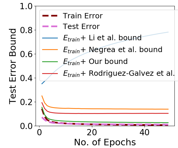
(a) MNIST, $\alpha_{t}^{2}\approx 0.1$

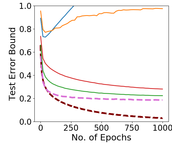
(b) CIFAR-10, $\alpha_{t}^{2}\approx 0.1$

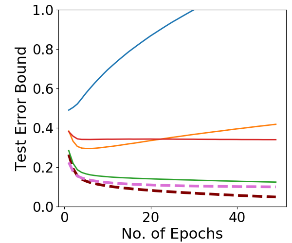
(c) Fashion, $\alpha_{t}^{2}\approx 0.1$

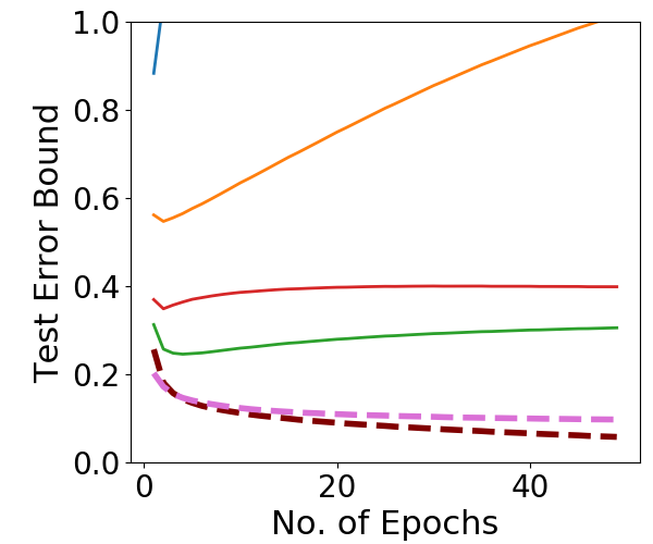
(d) Fashion, $\alpha_{t}^{2}\approx 0.01$

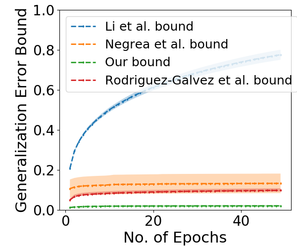
(e) MNIST, $\alpha_{t}^{2}\approx 0.1$

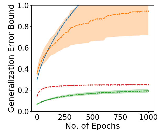
(f) CIFAR-10, $\alpha_{t}^{2}\approx 0.1$

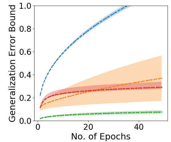
(g) Fashion, $\alpha_{t}^{2}\approx 0.1$

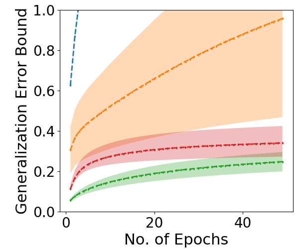
(h) Fashion, $\alpha_{t}^{2}\approx 0.01$

Figure 1: Results for training CNN using SGLD on MNIST, Fashion-MNIST and CIFAR-10. (a)-(d) shows our bound is non-vacuous and can be used to bound the empirical test error. (e)-(h) compare our bound with the existing bounds and show the effect on $\alpha_{t}^{2}$. Our bounds are numerically sharper than existing bounds, and larger $\alpha_{t}^{2}$ leads to tighter generalization bounds which is consistent with Theorem 2.

Stochastic Gradient Langevin Dynamics (SGLD). We acknowledge that following optimization result for SGLD exists in various forms, as noisy gradient descent algorithms with Gaussian noise have been studied in literature such as differential privacy, where SGLD can be viewed as DP-SGD (Bassily et al.,, 2014; Wang and Xu,, 2019) and the proof technique boils down to bounding the stochastic variance of the noisy gradient (Shamir and Zhang,, 2013).

Theorem 4.

The following holds for any $S$, any initialization $\mathbf{w}_{0}$, and the expectation is taken over the randomness of algorithm: under Assumptions 1 and 2 with $K_{i}=K,\forall i\in[p]$, SGLD, i.e., EFLD with Gaussian noise, $\rho_{t}=\eta_{t}$, $\alpha_{t}=\sigma_{t}/\eta_{t}$, and step size $\eta_{t}=\frac{1}{\sqrt{T}}$ satisfies

$$\mathbb{E}\|\nabla L_{S}(\mathbf{w}_{R})\|^{2}\leq O\left(\frac{1}{\sqrt{T}}\right)+O\left(\frac{\frac{K}{2T}\sum_{t=1}^{T}(p\alpha_{t}^{2}+\kappa_{t}^{2})}{\sqrt{T}}\right)~{},$$

where $\mathbf{w}_{R}$ is uniformly randomly sampled from $\{\mathbf{w}_{t}\}_{t=1}^{T}$.

The error rate of SGLD depends on the noise level $\alpha_{t}$ and the sub-Gaussian parameter $\kappa_{t}$. The bound has a $O(1/\sqrt{T})$ rate as long as the average noise level and sub-Gaussian parameter are bounded by a constant. Similar to differentially private SGD, the convergence rate depends on the dimension of the gradient $p$ due to the isotropic Gaussian noise. Special noise structures such as anisotropic noise that align with the gradient structure can improve the dependence on dimension (Kairouz et al.,, 2020; Zhang et al.,, 2021; Asi et al.,, 2021; Zhou et al.,, 2020).

4 Experiments

In this section, we conduct experiments to evaluate our generalization error bounds. For SGLD, we compare our bound in Theorem 2 with existing bounds in Li et al., (2020); Negrea et al., (2019); Rodríguez-Gálvez et al., (2021) for various datasets. Note that the bound presented in Rodríguez-Gálvez et al., (2021) is an extension of that in Haghifam et al., (2020) from full-batch setting to mini-batch setting. We also evaluate the optimization performance of proposed Noisy Sign-SGD, comparing it with the original Sign-SGD (Bernstein et al., 2018a, ) and present the corresponding generalization bound in Theorem 2.

The details of model architectures, learning rate schedules, hyper-parameter selections, and additional experimental results can be found in Appendix E. Evaluation of the expectation in Theorem 2 is done based on (re)sampling (Appendix E). We emphasize that the goal for the experiments is to do a comparative study relative to existing bounds. We note that the empirical performance of the methods can potentially be improved with better architectures and training strategies, e.g., deeper/wider networks, data augmentation, batch/layer normalization, etc.

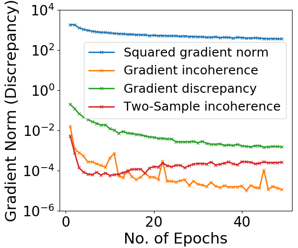
(a) MNIST, $\alpha_{t}^{2}\approx 0.1$

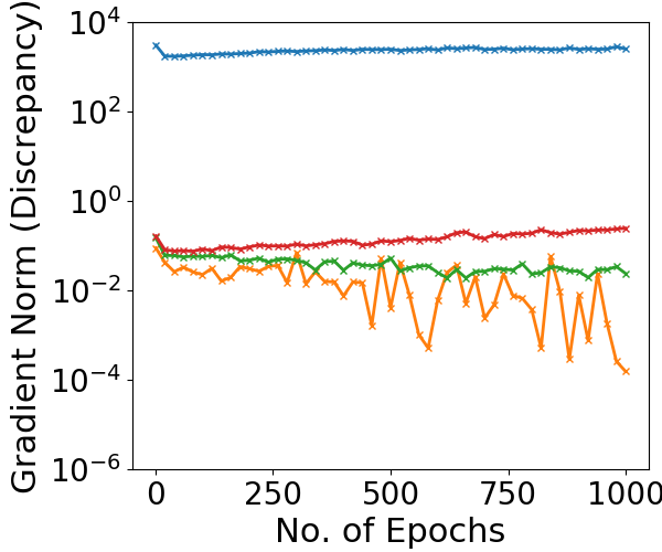
(b) CIFAR-10, $\alpha_{t}^{2}\approx 0.1$

Figure 2: Comparison of the squared gradient norm Li et al., (2020), the gradient incoherence Negrea et al., (2019), the two-sample incoherence Rodríguez-Gálvez et al., (2021), and the gradient discrepancy in our bound. Incoherence or discrepancy based quantities are orders of magnitude smaller than the gradient norm.

4.1 Stochastic Gradient Langevin Dynamics

Comparison with existing work. We have derived generalization error bounds that depend on the data-dependent gradient discrepancy, i.e., $\left\|\nabla\ell\left(\mathbf{w}_{t},z_{n}\right)-\nabla\ell\left(\mathbf{w}_{t},z^{\prime}_{n}\right)\right\|_{2}^{2}$. Existing bounds in Li et al., (2020) and Negrea et al., (2019) have also improved the Lipschitz constant in Mou et al., (2018) to a data-dependent quantity. All these generalization error bounds can be added to the empirical training error to get bounds on the empirical test error. As shown in Figure 1 (a)-(d), our bound is able to generate a much tighter upper bound on the test error. The improvements is mainly due to the fact that we replace the squared gradient norm in Li et al., (2020), the squared norm of gradient incoherence in Negrea et al., (2019), and that of two-sample incoherence in Rodríguez-Gálvez et al., (2021) with the gradient discrepancy while maintaining a $1/n$ sample dependence. Figure 1 (e)-(h) shows that our bounds are much sharper than those of Li et al., (2020) because our gradient discrepancy norms (Figure 2) are usually 2-4 order of magnitude smaller than the squared gradient norms in Li et al., (2020). Our bounds are also sharper than those of Negrea et al., (2019) and Rodríguez-Gálvez et al., (2021) due to our $O(1/n)$ sample dependence compared to their $O(1/\sqrt{n})$ dependence. Although the gradient incoherence in Negrea et al., (2019) is can be about 1 to 2 order of magnitude smaller than the gradient discrepancy for simple problems such as MNIST (Figure 2(a)), the difference between the gradient incoherence and our gradient discrepancy reduces as the problem becomes harder (see results for CIFAR-10 in Figure 2(b)).

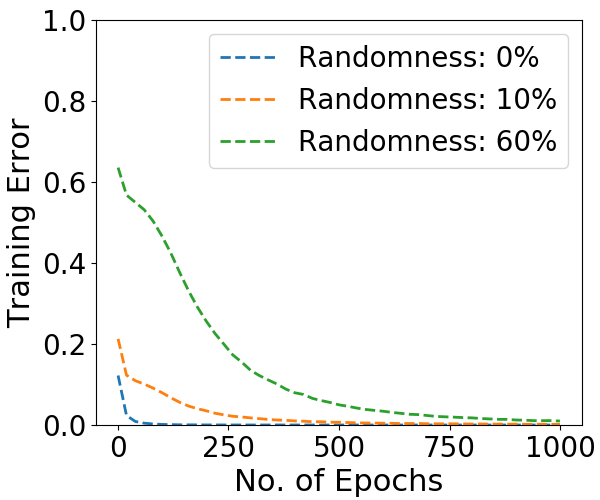
(a) Training Error

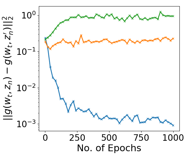
(b) Gradient Discrepancy

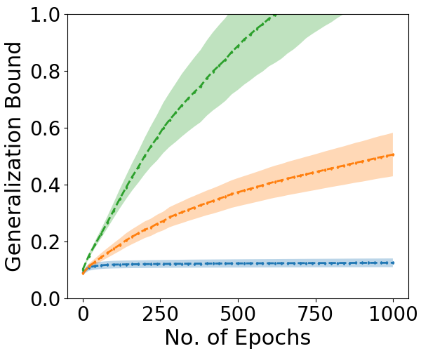
(c) Generalization Bound

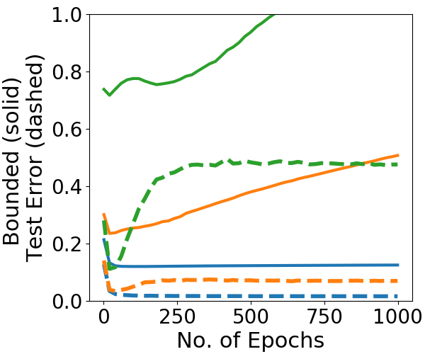
(d) Test Error Bound

Figure 3: Results for training CNN using SGLD on a subset of MNIST ($n=10000$) with different label randomness.(a) Training error: While training takes more epochs with random labels, training error does go to zero. (b) Gradient discrepancy: As the randomness increases, so does the gradient discrepancy, leading to the increase in the generalization bound. (c) Generalization bound: As the randomness increases, so does the generalization bound in Theorem 2. (d) Test error and bound: As the randomness increases, the empirical test error (dashed lines) increases and so does the test error bound (solid lines); overall, the bounds stay valid.

Effect of Random Labels. Motivated by Zhang et al., (2017), we train CNN with SGLD on a smaller subset of MNIST dataset ($n=10,000$) with randomly corrupted labels. The corruption fraction varies from $0\%$ (no label corruption) to $60\%$. As shown in Figure 3 (a), for long enough training time, all experiments with different levels of label randomness can achieve almost zero training error. However, increase in random labels leads to increase in gradient discrepancy (Figure 3(b)) which in turn leads to increase in the generalization bound (Figure 3(c)). As a result, as the empirical error rate increases with increase in label randomness (Figure 3(d) dashed lines), we get the correct increase in the test error bound (solid lines).

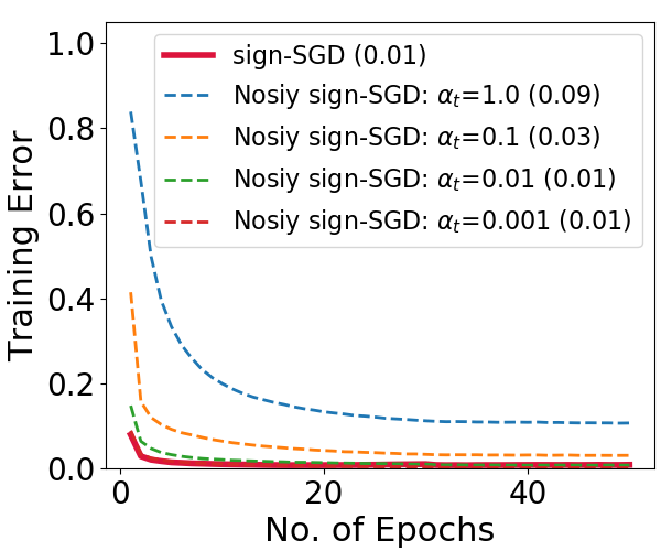
(a) CNN, MNIST

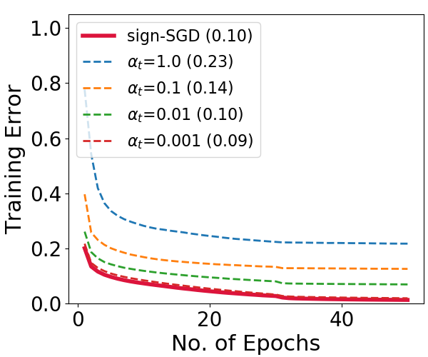
(b) CNN, Fashion

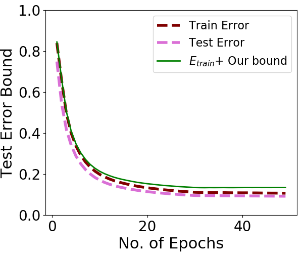
(c) CNN, MNIST, $\alpha_{t}=1$

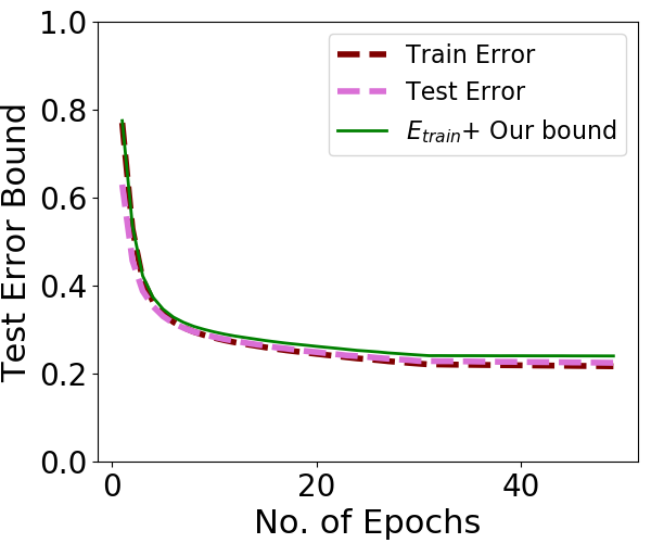
(d) CNN, Fashion, $\alpha_{t}=1$

Figure 4: (a)-(b) show the training dynamics of CNN on MNIST and Fashion-MNIST using noisy sign-SGD with different scaling $\alpha_{t}$. Legends indicate the choice of $\alpha_{t}$ and the numbers in brackets are test errors at convergence. As $\alpha_{t}\to 0$, Nosiy sign-SGD matches both the optimization trajectory as well as the final test accuracy of the original sign-SGD (Bernstein et al., 2018a, ). (c)-(d) show that empirical test error can be bounded by our bound and the corresponding training error.

4.2 Noisy Sign-SGD

In this section, we present numerical results for Noisy Sign-SGD proposed in section 3.1. Since none of the existing bounds can give a valid generalization bound for Noisy Sign-SGD, we only present our bound here.

Optimization. Figure 4 (a)-(b) show the training dynamics of Noisy Sign-SGD under various choices of $\alpha_{t}$. For small $\alpha_{t}$, Noisy Sign-SGD matches both the optimization trajectory as well as the test accuracy of the original Sign-SGD (Bernstein et al., 2018a, ). However, as $\alpha_{t}$ increases, the distribution over $\{-1,+1\}$ is more spread out and the corresponding Noisy Sign-SGD seems to converge but to a sub-optimal value.

Generalization Bound. Figure 4(c)-(d) show that our bound successfully bounds the empirical test error. Larger $\alpha_{t}$ leads to sharper generalization bounds. However, larger $\alpha_{t}$ adversely affects the optimization, e.g., Figure 4 (a)-(b) blue and orange lines. The results illustrate the trade-off between the empirical optimization and the generalization bound. In practice, one needs to balance the optimization error and generalization by choosing a suitable scaling $\alpha_{t}$.

5 Conclusions

Inspired by recent advances in stability based and information theoretic approaches to generalization bounds (Mou et al.,, 2018; Pensia et al.,, 2018; Negrea et al.,, 2019; Li et al.,, 2020; Haghifam et al.,, 2020), we have presented a framework for developing such bounds based on expected stability for noisy stochastic iterative algorithms. We have also introduced Exponential Family Langevin Dynamics (EFLD), a large family of noisy gradient descent algorithms based on exponential family noise, including SGLD and Noisy Sign-SGD as two special cases. We have developed an expected stability based generalization bound applicable to any EFLD algorithm with a $O({1}/{n})$ sample dependence and a dependence on gradient discrepancy, rather than gradient norms. Further, we have provided optimization guarantees for special cases of EFLD, viz. Noisy Sign-SGD and SGLD. Our experiments on various benchmarks illustrate that our bounds are non-vacuous and quantitatively much sharper than existing bounds (Li et al.,, 2020; Negrea et al.,, 2019).

Acknowledgements. The research was supported by NSF grants IIS 21-31335, OAC 21-30835, DBI 20-21898, and a C3.ai research award. We would like to thank the reviewers for valuable comments and the Minnesota Supercomputing Institute (MSI) for computational resources and support.

Appendix A Related Work

Uniform stability. Uniform stability is a classical approach for bounding generalization error (Bousquet and Elisseeff,, 2002; Hardt et al.,, 2016; Bousquet et al.,, 2020; Shalev-Shwartz et al.,, 2009; Feldman and Vondrak,, 2018, 2019), pioneered by Rogers and Wagner, (1978); Devroye and Wagner, (1979). Recently, uniform stability has been used in analyzing the stability of stochastic gradient descent (SGD) (Hardt et al.,, 2016). Mou et al., (2018) prove the uniform stability of SGLD (Welling and Teh,, 2011; Raginsky et al.,, 2017) by showing that uniform stability can be bounded by the squared Hellinger distance, and further they establish discretized Fokker-Planck equations for analyzing the squared Hellinger distance. Then they provide uniform stability based generalization bounds for SGLD as $\frac{L}{n}\sqrt{\sum_{t}\eta^{2}_{t}/\sigma_{t}^{2}}$ which depends on $L$, the global Lipschitz constant for gradients, and the step size $\eta_{t}\leq\frac{\sigma_{t}\ln 2}{L}$ (Mou et al.,, 2018; Li et al.,, 2020). Recently, Li et al., (2020) followed up on Mou et al., (2018) and derived a data-dependent bound based on Bayes-stability, and got a bound of the form $\frac{c}{n}\sqrt{\sum_{t}\eta^{2}_{t}\mathbf{g}_{e}(t)/\sigma_{t}^{2}}$, where $\mathbf{g}_{e}(t)$ is the expected gradient norm square at step $t$. Their bound improves the Lipschitz constant $L$ to the expected gradient norm square. Recently, Farghly and Rebeschini, (2021) provided a time-independent bound for SGLD of the form $O(1/n+\eta^{1/2}d^{1/2})$ which requires the step size scales as $O(1/(n^{2}d))$ to obtain an $O(1/n)$ bound. Bassily et al., (2019) analyze the uniform stability of differentially private SGD (DP-SGD) for convex optimization by showing the gradient update is a non-expansive operation, which is the key fact in proving the stability of SGD (Hardt et al.,, 2016). The approach in Hardt et al., (2016) can extend to non-convex setting as well, however it requires fast decaying in step size as $\eta_{t}=O(1/t)$. Bassily et al., (2020) provide stability analysis of SGD for convex and non-smooth functions.

Information-theoretic bounds. Besides the works mentioned above, other theories of deriving generalization bounds for noisy iterative algorithms have been proposed via information-theoretic approaches (Russo and Zou,, 2016; Xu and Raginsky,, 2017). Such results show that the generalization error of any learning algorithm can be bounded as $O(\sqrt{I(S;W)/n})$, where $I(S;W)$ is the mutual information between the algorithm input $S$ and the algorithm output $W$. Recent work following this approach focus on bounding the mutual information for a broad class of iterative algorithms, including SGLD to obtain a $O(\sqrt{\log T/n})$ generalization bound by choosing $\eta_{t}=O(1/t)$, where $T$ is the total number of iterations (Pensia et al.,, 2018; Bu et al.,, 2019). Subsequent improvements to this technique were made by Negrea et al., (2019); Haghifam et al., (2020); Rodríguez-Gálvez et al., (2021) to prove data-dependent generalization bounds that do not depend on the Lipschitz constant of the loss function and obtain $\sqrt{\sum_{t}\eta_{t}/n}$ bounds. Especially, Haghifam et al., (2020); Zhou et al., (2021) introduce generalization bounds based on conditional mutual information inspired by Steinke and Zakynthinou, (2020), leading to tighter bounds than those based on mutual information, which was extended by Rodríguez-Gálvez et al., (2021) from full-batch gradient to stochastic setting. Recently, Wang et al., 2021b provided a bound for SGLD of the from $O(\frac{b}{n}\sum_{j=1}^{m}\sqrt{\sum_{t\in{{\cal T}}_{j}}\eta_{t}^{2}\textit{Var}(\mathbf{g}_{j}(t))/\sigma_{t}^{2}})$, where $b$ is the mini-batch size, $m$ is the number of mini-batches, ${{\cal T}}_{j}$ contains the indices of iterations for mini-batch $S_{j}$ and $\textit{Var}(\mathbf{g}_{j}(t))$ is the variance of mini-batch gradient on $S_{j}$ evaluated on the training set. However, Wang et al., 2021b requires splitting training samples into disjoint $m$ mini-batches before training and obtained a bound dependending on the sum of gradient variance. Their bound also scales inversely to the batch size since the number of mini-batches $m$ and gradient variance increase as the batch size decreases. Neu et al., (2021) extend this information-theoretic approach to derive generalization bound for vanilla SGD. Hellström and Durisi, (2021) provide a fast-rate bound for bounded loss functions based via Conditional Information Measures (Grünwald et al.,, 2021; Hellström and Durisi,, 2020), which also provides a unified view of some of the above results.

Noisy iterative algorithms. Introducing additional noise in the stochastic gradient has been popular in training deep nets. Noisy iterative methods have proven to be useful for machine learning applications, especially for deep neural networks in terms of escaping from saddle points (Jin et al.,, 2017, 2019), preserving privacy (Bassily et al.,, 2020; Wang and Xu,, 2019), boosting generalization and stability (Mou et al.,, 2018; Li et al.,, 2020). SGLD (Welling and Teh,, 2011) has been one of the most popular noisy iterative algorithms for non-convex learning problems, where an isotropic Gaussian noise is added to the stochastic gradient. There has been some work (Wang et al.,, 2015; Li et al.,, 2019) connecting SGLD with differentially private SGD algorithm (DP-SGD) (Bassily et al.,, 2020; Wang and Xu,, 2019) which usually adds noise with constant variance to the stochastic gradient. Uniform stability has also been popular in the differential privacy literature for analyzing the generalization error bound of DP-SGD algorithms. Recently, noise has been proven to be useful in Sign-SGD (Bernstein et al., 2018a, ; Bernstein et al., 2018b, ; Chen et al.,, 2019) which has gained popularity as it reduces communication cost in distributed learning. Existing versions of noisy sign-SGD first adds symmetric noise to the stochastic gradient, then take the sign of the noisy stochastic gradient to update the parameters (Chen et al.,, 2019; Jin et al.,, 2020). Bernstein et al., 2018b ; Chen et al., (2019); Jin et al., (2020) have shown that when noise is unimodal and symmetric, sign-SGD can guarantee convergence to stationary point. Recently, Wang et al., 2021a study the anisotropic noise for SGLD, where they optimize the information-theoretical generalization bound by manipulating the noise structure in SGLD. They prove that with constraint to guarantee low empirical risk, the optimal noise covariance is the square root of the expected gradient covariance. In recent work, Lei and Ying, (2020) considered “on average stability” based generalization bounds, which is related to our work. Their bound has a dependence either on $L$ or on some form of convexity.

Appendix B Analysis and Proofs for Expected Stability (Section 2)

See 1

Proof.

Let $S_{n}=\left(z_{1},\ldots,z_{n}\right)$ and $\tilde{S}^{\prime}_{n}=\left(z_{1}^{\prime},\ldots,z_{n}^{\prime}\right)$ two independent random samples and let $S^{(i)}_{n}=\left(z_{1},\ldots,z_{i-1},z_{i}^{\prime},z_{i+1},\ldots,z_{n}\right)$ be the sample that is identical to $S$ except in the $i$-th example where we replace $z_{i}$ with $z_{i}^{\prime}$. Note that $S^{(n)}=S^{\prime}_{n}$ where $S^{\prime}_{n}$ is the dataset obtained by replacing $z_{n}\in S_{n}$ with $z^{\prime}_{n}$ as in the Proposition statement. Now, by definition we have

$$\left|\mathbb{E}_{S_{n}\sim D^{n}}[L_{D}(A(S_{n}))-L_{S}(A(S_{n}))]\right|$$

$$=\left|\mathbb{E}_{S_{n}\sim D^{n}}[L_{S}(A(S_{n}))-L_{D}(A(S_{n}))]\right|$$

$$=\left|\mathbb{E}_{S_{n}}\mathbb{E}_{\tilde{S}_{n}^{\prime}}\mathbb{E}_{A}\left[\frac{1}{n}\sum_{i=1}^{n}\left(\ell(A(S_{n}^{(i)}),z_{i}^{\prime})-\ell(A(S_{n}),z_{i}^{\prime})\right)\right]\right|$$

$$=\left|\mathbb{E}_{S_{n}}\mathbb{E}_{\tilde{S}_{n}^{\prime}}\frac{1}{n}\sum_{i=1}^{n}\mathbb{E}_{A}\left[\ell(A(S_{n}^{(i)}),z_{i}^{\prime})-\ell(A(S_{n}),z_{i}^{\prime})\right]\right|$$

$$\overset{(a)}{=}\left|\mathbb{E}_{S_{n}}\mathbb{E}_{\tilde{S}_{n}^{\prime}}\frac{1}{n}\sum_{i=1}^{n}\left(\int_{\mathbb{R}^{d}}\ell(\mathbf{w};z_{i}^{\prime})p^{(i)}(\mathbf{w})d\mathbf{w}-\int_{\mathbb{R}^{d}}\ell(\mathbf{w};z_{i}^{\prime})p(\mathbf{w})d\mathbf{w}\right)\right|$$

$$=\left|\mathbb{E}_{S_{n}}\mathbb{E}_{\tilde{S}_{n}^{\prime}}\frac{1}{n}\sum_{i=1}^{n}\int_{\mathbb{R}^{d}}\ell(\mathbf{w};z_{i}^{\prime})\left(p^{(i)}(\mathbf{w})-p(\mathbf{w})\right)d\mathbf{w}\right|$$

$$=\left|\mathbb{E}_{S_{n}}\mathbb{E}_{\tilde{S}_{n}^{\prime}}\frac{1}{n}\sum_{i=1}^{n}\int_{\mathbb{R}^{d}}\ell(\mathbf{w};z_{i}^{\prime})\left(\sqrt{p^{(i)}(\mathbf{w})}+\sqrt{p(\mathbf{w})}\right)\left(\sqrt{p^{(i)}(\mathbf{w})}-\sqrt{p(\mathbf{w})}\right)d\mathbf{w}\right|$$

$$\overset{(b)}{\leq}\left|\mathbb{E}_{S_{n}}\mathbb{E}_{\tilde{S}_{n}^{\prime}}\frac{1}{n}\sum_{i=1}^{n}\left\{\left(\int_{\mathbb{R}^{d}}\ell^{2}(\mathbf{w};z_{i}^{\prime})\left(\sqrt{p^{(i)}(\mathbf{w})}+\sqrt{p(\mathbf{w})}\right)^{2}d\mathbf{w}\right)^{\frac{1}{2}}\left(\int_{\mathbb{R}^{d}}\left(\sqrt{p^{(i)}(\mathbf{w})}-\sqrt{p(\mathbf{w})}\right)^{2}d\mathbf{w}\right)^{\frac{1}{2}}\right\}\right|$$

where in (a) $p^{(i)}(\mathbf{w}),p(\mathbf{w})$ are respectively the distributions obtained by $A(S_{n}^{(i)}),A(S_{n})$, and (b) follows by Cauchy-Schwartz inequality. Focusing on the first integral, we have:

$$\left(\int_{\mathbb{R}^{d}}\ell^{2}(\mathbf{w};z_{i}^{\prime})\left(\sqrt{p^{(i)}(\mathbf{w})}+\sqrt{p(\mathbf{w})}\right)^{2}d\mathbf{w}\right)^{1/2} \leq\left(2\int_{\mathbb{R}^{d}}\ell^{2}(\mathbf{w};z_{i}^{\prime})p^{(i)}(\mathbf{w})d\mathbf{w}+2\int_{\mathbb{R}^{d}}\ell^{2}(\mathbf{w};z_{i}^{\prime})p(\mathbf{w})d\mathbf{w}\right)^{1/2}$$

$$\leq\left(c_{0}^{2}/2+c_{0}^{2}/2\right)^{1/2}=c_{0}~{}.$$

Hence, by definition of the Hellinger divergence, we have

$$\mathbb{E}_{S_{n}\sim D^{n}}[L_{D}(A(S_{n}))-L_{S}(A(S_{n}))] \leq\mathbb{E}_{S_{n}}\mathbb{E}_{\tilde{S_{n}}^{\prime}}\frac{1}{n}\sum_{i=1}^{n}c_{0}\sqrt{2H^{2}\left(A(S_{n}),A(S_{n}^{(i)})\right)}$$

$$\overset{(a)}{=}\mathbb{E}_{S_{n}}\mathbb{E}_{\tilde{S}_{n}^{\prime}}\frac{1}{n}\sum_{i=1}^{n}c_{0}\sqrt{2H^{2}\left(A(S_{n}),A(S^{\prime}_{n})\right)}$$

$$=c_{0}\mathbb{E}_{S_{n}\sim D^{n}}\mathbb{E}_{z^{\prime}_{n}\sim D}\sqrt{2H^{2}\big{(}A(S_{n}),A(S^{\prime}_{n})\big{)}}~{},$$

where (a) follows since the samples are drawn i.i.d. and the randomized algorithm $A(\cdot)$ is permutation invariant. That completes the proof. ∎

Proposition 2.

For any distributions $P$ and $P^{\prime}$, $2H^{2}(P,P^{\prime})\leq\min\big{\{}KL(P,P^{\prime}),\sqrt{\frac{1}{2}KL(P,P^{\prime})}\big{\}}$.

Proof.

For the first part, note that:

$$KL(P,P^{\prime}) =\int\left(\log\frac{p(\mathbf{w})}{p^{\prime}(\mathbf{w})}\right)p(\mathbf{w})~{}d\mathbf{w}$$

$$=2\int\left(-\log\sqrt{\frac{p^{\prime}(\mathbf{w})}{p(\mathbf{w})}}\right)p(\mathbf{w})~{}d\mathbf{w}$$

$$\overset{(a)}{\geq}2\int\left(1-\sqrt{\frac{p^{\prime}(\mathbf{w})}{p(\mathbf{w})}}\right)p(\mathbf{w})~{}d\mathbf{w}$$

$$=2\int\left(p(\mathbf{w})-\sqrt{p(\mathbf{w})p^{\prime}(\mathbf{w})})\right)~{}d\mathbf{w}$$

$$=\int\left(p(\mathbf{w})+p^{\prime}(\mathbf{w})-2\sqrt{p(\mathbf{w})p^{\prime}(\mathbf{w})}\right)~{}d\mathbf{w}$$

$$=\int\left(\sqrt{p(\mathbf{w})}-\sqrt{p^{\prime}(\mathbf{w})}\right)^{2}~{}d\mathbf{w}$$

$$=2H^{2}(P,P^{\prime})~{},$$

where (a) follows since for $z>-1$, $\log(1+z)\leq z$, using $x=1+z$ and changing signs gives $-\log x\geq 1-x$.

For the second part, note that:

$$2H^{2}(P,P^{\prime}) =\int_{\mathbf{w}}(\sqrt{p(\mathbf{w})}-\sqrt{p^{\prime}(\mathbf{w})})^{2}d\mathbf{w}$$

$$=\int_{\mathbf{w}}|\sqrt{p(\mathbf{w})}-\sqrt{p^{\prime}(\mathbf{w})}|\times|\sqrt{p(\mathbf{w})}-\sqrt{p^{\prime}(\mathbf{w})}|~{}d\mathbf{w}$$

$$\leq\int_{\mathbf{w}}|\sqrt{p(\mathbf{w})}-\sqrt{p^{\prime}(\mathbf{w})}|\times|\sqrt{p(\mathbf{w})}+\sqrt{p^{\prime}(\mathbf{w})}|~{}d\mathbf{w}$$

$$=\int_{\mathbf{w}}|p(\mathbf{w})-p^{\prime}(\mathbf{w})|~{}d\mathbf{w}$$

$$=TV(P,P^{\prime})~{},$$

where $TV(P,P^{\prime})$ denotes the total variation distance (Pollard,, 2002). Further, from Pinsker’s inequality (Tsybakov,, 2008), we have

$$TV(P,P^{\prime})\leq\sqrt{\frac{1}{2}KL(P,P^{\prime})}~{}.$$

Combining the two results completes the proof. ∎

B.1 Proofs for Section 2.2

Our first result establishes a bound on the KL-divergence between two component mixture models in terms of the mixing weight of the unique components. Similar results have appeared in (Li et al.,, 2020; Bun et al.,, 2018) in related contexts. Our proof is different, simple, and self-contained.

Lemma 4.

Let $Q,Q^{\prime},R$ be any three distributions such that $Q,Q^{\prime}$ are both absolutely continuous w.r.t. $R$. Then, for any $s\in(0,1)$

$$KL\left(sQ+(1-s)R~{}\big{\|}~{}sQ^{\prime}+(1-s)R\right)\leq\frac{s^{2}}{1-s}~{}\int_{\mathbf{w}}\frac{(Q(\mathbf{w})-Q^{\prime}(\mathbf{w}))^{2}}{R(\mathbf{w})}d\mathbf{w}~{}.$$ (19)

Proof.

Let $U=sQ^{\prime}+(1-s)R$. Then, with $F(x)=Q(x)-Q^{\prime}(x)$, we have

$$KL(sQ+(1-s)R\|sQ^{\prime}+(1-s)R) =KL(U+s(Q-Q^{\prime})\|U)$$

$$=\int(U(x)+sF(x))\log\left(\frac{U(x)+sF(x)}{U(x)}\right)dx$$

$$=\int(U(x)+sF(x))\log\left(1+\frac{sF(x)}{U(x)}\right)dx$$

$$=\int sF(x)+\frac{s^{2}F^{2}(x)}{2U(x)}-\frac{s^{3}F^{3}(x)}{6U^{2}(x)}+\frac{s^{4}F^{4}(x)}{12U^{3}(x)}-\cdots dx$$

$$=s^{2}\int\frac{F^{2}(x)}{U(x)}\left(\frac{1}{2}-\frac{sF(x)}{6U(x)}+\frac{s^{2}F^{2}(x)}{12U^{2}(x)}-\cdots\right)dx~{},$$

where the first term vanishes since $\int F(x)dx=\int(Q(x)-Q^{\prime}(x))dx=0$. This is the reason the dependency is on $s^{2}$, not $s$. With $W(x)=sF(x)/U(x)$, noting that $W(x)>-1$, and

$$\left(\frac{1}{2}-\frac{W(x)}{6}+\frac{W^{2}(x)}{12}-\cdots\right)=\frac{(1+W(x))\log(1+W(x))-W(x)}{W^{2}(x)}\leq 1~{},$$ (20)

we have

$$KL(sP+(1-s)R\|sQ+(1-s)R) =s^{2}\int\frac{F^{2}(x)}{U(x)}\left(\frac{(1+W(x))\log(1+W(x))-W(x)}{W^{2}(x)}\right)dx$$

$$\leq s^{2}\int\frac{F^{2}(x)}{U(x)}dx~{}$$

$$\leq\frac{s^{2}}{(1-s)}\int\frac{(Q(x)-Q^{\prime}(x))^{2}}{R(x)}dx~{}.$$

That completes the proof. ∎

Proposition 3.

Consider the mixture models $Q_{t|}=\frac{1}{|G_{1}|}\sum_{B_{t}\in G_{1}}P_{B_{t},\bm{\xi}_{t}}$, $Q^{\prime}_{t|}=\frac{1}{|G_{1}|}\sum_{B_{t}\in G_{1}}P^{\prime}_{B_{t},\bm{\xi}_{t}}$, $R_{t}=\frac{1}{|G_{0}|}\sum_{A_{t}\in G_{0}}P_{A_{t},\bm{\xi}_{t}}$. Then, with $s=\frac{|G_{1}|}{|G|}=\frac{\binom{n-1}{b-1}}{\binom{n}{b}}=\frac{b}{n}$, we have

$$P_{t|}=sQ_{t|}+(1-s)R_{t|}~{},\qquad\text{and}\qquad P^{\prime}_{t|}=sQ^{\prime}_{t|}+(1-s)R_{t|}~{}.$$

Proof.

The proof follows the argument in the proof of Lemma 21 in Li et al., (2020).∎

Lemma 5.

Consider a general noisy stochastic iterative algorithm with updates of the form (5) with mini-batch size $B_{t}=b$. Then, conditioned on any trajectory $\mathbf{w}_{0:t-1}$, we have

$$KL\left(P_{t|}\|P_{t|}\right)\leq\frac{b^{2}}{n^{2}}\frac{n}{n-b}\mathbb{E}_{B_{t}\in G_{1}}\mathbb{E}_{A_{t}\in G_{0}}\left[\bigintsss_{\bm{\xi}_{t}}\frac{\left(dP_{B_{t},\bm{\xi}_{t}}-dP^{\prime}_{B_{t},\bm{\xi}_{t}}\right)^{2}}{dP_{A_{t},\bm{\xi}_{t}}}d\bm{\xi}_{t}\right]~{}.$$ (21)

Proof.

By definition, Proposition 3, and Lemma 4 with $s=b/n$, we have

$$KL\left(P_{t|}\|P^{\prime}_{t|}\right) \stackrel{{\scriptstyle(a)}}{{\leq}}\left(\frac{b}{n}\right)^{2}\left(\frac{n}{n-b}\right)\int_{\mathbf{w}}\frac{(Q-Q^{\prime})^{2}}{R}d\mathbf{w}$$

$$=\frac{b^{2}}{n^{2}}\left(1+\frac{b}{n-b}\right)\bigintsss_{\mathbf{w}}\frac{\left(\frac{1}{|G_{1}|}\left[\sum_{B\in G_{1}}dP_{B,\bm{\xi}}(\mathbf{w})-\sum_{B\in G_{1}}P^{\prime}_{B,\bm{\xi}}(\mathbf{w})\right]\right)^{2}}{\frac{1}{|G_{0}|}\sum_{A\in G_{0}}dP_{A,\bm{\xi}}(\mathbf{w})}d\mathbf{w}$$

$$\stackrel{{\scriptstyle(b)}}{{\leq}}\frac{b^{2}}{n^{2}}\left(1+\frac{b}{n-b}\right)\bigintsss_{\mathbf{w}}\frac{1}{|G_{1}|}\sum_{B\in G_{1}}\frac{\left(dP_{B,\bm{\xi}}(\mathbf{w})-P^{\prime}_{B,\bm{\xi}}(\mathbf{w})\right)^{2}}{\frac{1}{|G_{0}|}\sum_{A\in G_{0}}dP_{A,\bm{\xi}}(\mathbf{w})}d\mathbf{w}$$

$$\stackrel{{\scriptstyle(c)}}{{\leq}}\frac{b^{2}}{n^{2}}\left(1+\frac{b}{n-b}\right)\bigintsss_{\mathbf{w}}\frac{1}{|G_{1}|}\sum_{B\in G_{1}}\left\{\left(dP_{B,\bm{\xi}}(\mathbf{w})-P^{\prime}_{B,\bm{\xi}}(\mathbf{w})\right)^{2}\frac{1}{|G_{0}|}\sum_{A\in G_{0}}\frac{1}{dP_{A,\bm{\xi}}(\mathbf{w})}\right\}d\mathbf{w}$$

$$=\frac{b^{2}}{n^{2}}\left(1+\frac{b}{n-b}\right)\frac{1}{|G_{1}||G_{0}|}\sum_{B\in G_{1}}\sum_{A\in G_{0}}\bigintsss_{\mathbf{w}}\frac{\left(dP_{B,\bm{\xi}}(\mathbf{w})-P^{\prime}_{B,\bm{\xi}}(\mathbf{w})\right)^{2}}{dP_{A,\bm{\xi}}(\mathbf{w})}d\mathbf{w}~{},$$

where (a) is from Lemma 4, (b)(c) is from Jensen’s inequality since function $f(x)=x^{2}$ is convex and $f(x)=\frac{1}{x}$ is convex on $(0,\infty)$. That completes the proof. ∎

Now we have all the pieces to prove the following result:

See 1

Proof.

Based on Propositions 4 and 2, we have

$$\mathbb{E}_{S\sim D^{n}}[L_{D}(A(S))-L_{S}(A(S))] \leq\sqrt{KL\left(P_{T}\|P_{T}^{\prime}\right)}\leq\sqrt{\sum_{t=1}^{T}\mathbb{E}_{P_{0:(t-1)}}\left[KL\left(P_{t\mid}\|P_{t\mid}^{\prime}\right)\right]}$$

Applying Lemma 5 to bound $KL\left(P_{t\mid}\|P_{t\mid}^{\prime}\right)$ and noting that $b/(n-b)\leq 1$ for $b\leq n/2$ completes the proof. ∎

B.2 High Probability Generalization Bounds

Let $S\sim D^{n}$ with $S=(Z_{1}\ldots,Z_{n})$ corresponding to the training data. Consider the random variable $Y(S)$, the Scaled (by $n$) Generalization Error (SGE), defined as

$$Y(S)\triangleq\sum_{i=1}^{n}\mathbb{E}_{A}\big{[}\mathbb{E}_{Z\sim D}[\ell(A(S),Z)]-\ell(A(S),Z_{i})\big{]}=n\big{(}L_{D}(A(S))-L_{S}(A(S))\big{)}~{}.$$ (22)

Theorem 11 establishes a bound on $|\frac{1}{n}\mathbb{E}_{S}[Y(S)]|$. We now focus on establishing a high probability bound on $\frac{1}{n}(Y(S)-\mathbb{E}_{S}[Y(S)])$. Let $S^{\prime}=(Z^{\prime}_{1},\ldots,Z^{\prime}_{n})$ be such that $Z^{\prime}_{i}$ is an independent copy of $Z_{i}$. Further, let $S^{\prime}_{i}=(Z_{1},\ldots,Z_{i-1},Z^{\prime}_{i},Z_{i+1},\ldots,Z_{n})$. Then, the change in SGE

$$Y(S)-Y(S^{\prime}_{i})=n\big{[}\big{(}L_{D}(A(S))-L_{D}(A(S^{\prime}_{i}))\big{)}-\big{(}L_{S}(A(S))-L_{S^{\prime}_{i}}(A(S^{\prime}_{i})\big{)}\big{]}$$ (23)

is a symmetric random variable, and is identically distributed for $i=1,\ldots,n$. Our analysis is based on the following assumption:

Assumption 3.

The random variable $(Y(S)-Y(S^{\prime}_{i}))^{2}$ is sub-Gaussian with $\psi_{2}$-norm $\kappa_{A}^{2}$, i.e., $\|(Y-Y^{\prime}_{i})^{2}\|_{\psi_{2}}=\sup_{q\geq 1}(\mathbb{E}_{S.S^{\prime}}|Y(S)-Y(S^{\prime}_{i})|^{2q})^{1/q}/\sqrt{q}=\kappa_{A}^{2}$.

Assumption 3 implies that $\|Y-Y^{\prime}_{i}\|_{\psi_{2}}\leq\kappa_{A}$. Note that since $Y(S)-Y(S^{\prime}_{i})$ is identically distributed for all $i$, $\kappa_{A}$ is the same for all $i$. Further, $\kappa_{A}$ is a property of the algorithm $A$, and can be viewed as a measure of stability. If $\kappa_{A}=O(1)$, i.e., swapping one point effectively leads to $O(\frac{1}{n})$ change in the generalization error, then $A$ can be considered stable; on the other hand, if $\kappa_{A}=O(\sqrt{n})$, then $A$ is not stable since the effective change in generalization error $\frac{1}{n}(Y(S)-Y(S^{\prime}_{i}))$ is $O(1/\sqrt{n})$, the same order as typical generalization error $\frac{1}{n}Y(S)$ itself. The sharpness of the high-probability bound we present meaningfully depends on $\kappa_{A}$, with smaller values implying sharper bounds.

Theorem 5.

Under Assumption 3, with probability at least $(1-\delta)$ over the draw $S\sim D^{n}$, we have

$$L_{D}(A(S))\leq L_{S}(A(S))+\mathbb{E}_{S}\bigg{[}L_{D}(A(S)-L_{S}(A(S))\bigg{]}+\max\left(\frac{1}{n},\frac{c_{1}\kappa_{A}}{\sqrt{n}}\right)\log\left(\frac{16}{\delta}\right)~{}.$$ (24)

If $\kappa_{A}=O(1)$, i.e., swapping one point effectively leads to $O(\frac{1}{n})$ change in the generalization error, then $A$ can be considered very stable; if $\kappa_{A}=O(\sqrt[4]{n})$, then $A$ can be considered somewhat stable; and if $\kappa^{2}_{A}=O(\sqrt{n})$, then $A$ is not stable since the effective change in generalization error $\frac{1}{n}(Y(S)-Y(S^{\prime}_{i}))$ is $O(1/\sqrt{n})$, the same order as the generalization error $\frac{1}{n}Y(S)$ itself.

Proof.

Let $S=(Z_{1},\ldots,Z_{n})$ and let $S^{\prime}=(Z^{\prime}_{1},\ldots,Z^{\prime}_{n})$ be such that $Z^{\prime}_{i}$ is an independent copy of $Z_{i}$. With $(x)_{+}=max(x,0)$, let

$$V^{+}=V^{+}(S)=\sum_{i=1}^{n}\mathbb{E}_{S^{\prime}}[(Y-Y^{\prime}_{i})_{+}^{2}]~{},$$ (25)

Our proof uses the following exponential version of the Efron-Stein inequality [Theorem 6.16 in Boucheron et al., (2013)], whose proof is based on a combination of the symmetric modified log-Sobolev inequality [Theorem 6.15 in Boucheron et al., (2013)] with the change of measure:

Theorem 6.

Let $Y=f(Z_{1},\ldots,Z_{n})$, where $Z_{i},i=1,\ldots,n$ are independent. Let $\theta,\lambda>0$ be such that $\theta\lambda<1$ and $\mathbb{E}[\exp(\lambda V^{+}/\theta)]<\infty$. Then,

$$\log\mathbb{E}\left[e^{\lambda(Y-\mathbb{E}Y)}\right]\leq\frac{\lambda\theta}{1-\lambda\theta}\log\mathbb{E}\left[e^{\lambda V^{+}/\theta}\right]~{}.$$ (26)

For the proof of Theorem 24, note that $V^{+}$ is sub-Gaussian with $\|V^{+}\|_{\psi_{2}}\leq n\kappa_{A}^{2}$. Let $\mu_{+}=\mathbb{E}[V^{+}]$ and $\kappa_{+}=\|V^{+}\|_{\psi_{2}}$. Then from Theorem 6, we have

$$\psi(\lambda)\triangleq\log\mathbb{E}\left[e^{\lambda(Y-\mathbb{E}Y)}\right]\leq\frac{\lambda\theta}{1-\lambda\theta}\left[\frac{\lambda\mu_{+}}{\theta}+c\frac{\lambda^{2}\kappa_{+}^{2}}{\theta^{2}}\right].$$

Then, by Markov’s inequality we have

$$\log\mathbb{P}(Y-\mathbb{E}Y>t) \leq\psi(\lambda)-\lambda t$$

$$\leq\frac{1}{1-\lambda\theta}\left[\lambda^{2}\mu_{+}+c\lambda^{3}\kappa_{+}^{2}/\theta-(1-\lambda\theta)\lambda t\right]~{}.$$

Choosing $\theta=1/(2\lambda)$, we have

$$\log\mathbb{P}(Y-\mathbb{E}Y>t) \leq 2\lambda^{2}\mu_{+}+4c\lambda^{4}\kappa_{+}^{2}-\lambda t~{}.$$

Consider choosing $\lambda=\min\left\{1,\frac{1}{c_{0}\sqrt{2\kappa_{+}}}\right\}$, where $c_{0}=\max(1,\sqrt[4]{c})$. Since $\mu_{+}\leq\kappa_{+}$, we have

$$\log\mathbb{P}(Y-\mathbb{E}Y>t) \leq 2-\min\left\{1,\frac{1}{c_{0}\sqrt{2\kappa_{+}}}\right\}t$$

$$\Rightarrow\quad\mathbb{P}(Y-\mathbb{E}Y>t) \leq 8\exp\left(-\min\left\{1,\frac{1}{c_{0}\sqrt{2\kappa_{+}}}\right\}t\right)~{}.$$

With $t=n\epsilon$, and noting that $\kappa_{+}\leq n\kappa_{A}^{2}$, with $c_{1}=c_{0}\sqrt{2}$, we have

$$\mathbb{P}\left(Y-\mathbb{E}Y>n\epsilon\right) \leq 8\exp\left(-\min\left\{n,\frac{\sqrt{n}}{c_{1}\kappa_{A}}\right\}\epsilon\right)~{}.$$

Now, we choose $\delta$ such that

$$8\exp\left(-\min\left\{n,\frac{\sqrt{n}}{c_{1}\kappa_{A}}\right\}\epsilon\right)\leq 8\exp\left(-n\epsilon\right)+8\exp\left(-\frac{\sqrt{n}}{c_{1}\kappa_{A}}\epsilon\right)\leq\delta~{}.$$

It suffices to choose $\epsilon$ such that

$$8\exp\left(-n\epsilon\right)\leq\delta/2 \qquad\Rightarrow\qquad\epsilon\geq\frac{1}{n}\log\left(\frac{16}{\delta}\right)$$

$$8\exp\left(-\frac{\sqrt{n}}{c_{1}\kappa_{A}}\epsilon\right)\leq\delta/2 \qquad\Rightarrow\qquad\epsilon\geq\frac{c_{1}\kappa_{A}}{\sqrt{n}}\log\left(\frac{16}{\delta}\right)~{}.$$

As a result,

$$\mathbb{P}\left(\frac{1}{n}(Y-\mathbb{E}Y)>\max\left(\frac{1}{n},\frac{c_{1}\kappa_{A}}{\sqrt{n}}\right)\log\left(\frac{16}{\delta}\right)\right) \leq\delta~{}.$$

That completes the proof. ∎

Appendix C Analysis and Proofs for EFLD (Section 3)

In this section, we provide the proofs for Section 3. We first review and show details of a few examples of exponential family.

C.1 Examples of Exponential Family

We show that EFLD becomes SGLD when the exponential family is Gaussian, and becomes a noisy version of sign-SGD (Bernstein et al., 2018a, ; Bernstein et al., 2018b, ) when the exponential family is skewed over $\{-1,+1\}$.

Example C.1 (Gaussian).

SGLD uses scaled Gaussian noise with $\psi(\bm{\theta})=\|\bm{\theta}\|_{2}^{2}/2,\alpha_{t}=\sigma_{t}/\eta_{t}$, $\bm{\pi}_{0,\alpha_{t}}(\bm{\xi})=\frac{1}{\sqrt{(2\pi)^{p}\alpha_{t}^{p}}}\exp(-\|\bm{\xi}\|_{2}^{2}/2\alpha_{t}^{2})$ so that $p_{\psi}(\bm{\xi};\bm{\theta}_{B_{t},\alpha_{t}})=\mathcal{N}(\bm{\theta}_{B_{t}},\alpha_{t}^{2}\mathbb{I}_{d})$. Then, the distribution from the natural parameter form is:

$$p_{\bm{\theta}/\sigma}(\xi)=\exp(\langle\xi,\bm{\theta}\rangle/\sigma^{2}-\|\theta\|_{2}^{2}/(2\sigma^{2}))\times\frac{1}{\sqrt{2\pi}\sigma}\exp(-\|\xi\|_{2}^{2}/2\sigma^{2})=\frac{1}{\sqrt{2\pi}\sigma}\exp(-\|\bm{\xi}-\bm{\mu}\|_{2}^{2}/2\sigma^{2})~{}.$$ (27)

The expectation parameter $\bm{\mu}=\nabla\psi(\bm{\theta})=\bm{\theta}$. The scaled expectation parameter $\bm{\mu}_{\alpha}=\nabla\psi(\bm{\theta}_{\alpha})=\bm{\theta}_{\alpha}=\bm{\theta}/\sigma=\bm{\mu}/\sigma$. Since $\xi=x/\sigma$ and the Bregman divergence $d_{\phi}(\bm{\xi},\bm{\mu})=\frac{1}{2}\|\bm{\xi}-\bm{\mu}\|_{2}^{2}$, the expectation parameter form

$$p_{\bm{\mu}_{\alpha}}(\bm{\xi})=\exp(-\|\bm{\xi}/\sigma-\bm{\mu}/\sigma\|_{2}^{2}/2)\frac{1}{\sqrt{2\pi}\sigma}=\frac{1}{\sqrt{2\pi}\sigma}\exp(-\|\bm{\xi}-\bm{\mu}\|_{2}^{2}/2\sigma^{2})~{}.$$ (28)

By taking $\rho_{t}=\eta_{t}$, the update (13) based on $\rho_{t}\bm{\xi}_{t}$ is distributed as $\mathcal{N}(\eta_{t}\bm{\theta}_{B_{t}},\eta_{t}^{2}\alpha_{t}^{2}\mathbb{I}_{d})=\mathcal{N}(\eta_{t}\nabla\ell(\mathbf{w}_{t-1},S_{B_{t}}),\sigma_{t}^{2}\mathbb{I}_{d})$. Thus the EFLD update reduces to the SGLD update: $\mathbf{w}_{t}=\mathbf{w}_{t-1}-\eta_{t}\nabla\ell(\mathbf{w}_{t-1},S_{B_{t}})+\mathcal{N}\left(0,\sigma_{t}^{2}\mathbb{I}_{d}\right).$ ∎

Example C.2 (Skewed Rademacher).

For skewed Rademacher over $\{-1,1\}$, the sufficient statistic $\xi\in\{-1,1\}$, base measure is 1 on $\{-1,1\}$, and the log-partition function $\psi(\theta)=\log(\exp(-\theta)+\exp(\theta))$ for natural parameter $\theta\in\mathbb{R}$. The expectation parameter $\mu=\nabla\psi(\theta)=\frac{\exp(\theta)-\exp(-\theta)}{\exp(-\theta)+\exp(\theta)}=\frac{\exp(2\theta)-1}{\exp(2\theta)+1}$, then its inverse function $\theta=\nabla\phi(\mu)=\frac{1}{2}\log\left(\frac{1+\mu}{1-\mu}\right)$, by integration we have $\phi(\mu)=\frac{1+\mu}{2}\log\frac{1+\mu}{2}+\frac{1-\mu}{2}\log\frac{1-\mu}{2}$. The expectation parameter $\mu=\nabla\psi(\theta)=\frac{\exp(\theta)}{1+\exp(\theta)}=\frac{1}{1+\exp(-\theta)}$, the sigmoid function of $\theta$. The Bregman divergence is the Bernoulli KL-divergence given by: $d_{\phi}(\xi,\mu)=\xi\log\frac{\xi}{\mu}+(1-\xi)\log\frac{1-\xi}{1-\mu}$. For scaled parameters $\theta_{\alpha}=\theta/\alpha$, the corresponding expectation parameter $\mu_{\alpha}=\frac{1}{1+\exp(-\theta_{\alpha})}$. The mean parameter form distribution is given by

$$p_{\mu_{\alpha}}(\xi)=\exp(-d_{\phi}(\xi,\mu_{\alpha}))=\mu_{\alpha}^{\xi}(1-\mu_{\alpha})^{1-\xi}~{}.$$ (29)

Noisy Sign-SGD takes $\rho_{t}=\eta_{t}$ and componentwise $\xi_{j}\in\{-1,1\},~{}\pi_{0,\alpha_{t}}(\xi_{j})=1,~{}\psi(\theta)=\log(\exp(-\theta)+\exp(\theta))$ in exponential family update equation (13), the $j$-th component of exponential family distribution $p_{\psi}(\bm{\xi};\bm{\theta}_{B_{t},\alpha_{t}})$ becomes

$$p_{\psi}(\xi_{j};\bm{\theta}_{B_{t},\alpha_{t},j})=\frac{\exp(\xi_{j}\bm{\theta}_{B_{t},\alpha_{t},j})}{\exp(-\theta_{B_{t},\alpha_{t},j})+\exp(\theta_{B_{t},\alpha_{t},j})}~{}.$$ (30)

Thus, the EFLD update reduces to a noisy version of Sign-SGD: $\mathbf{w}_{t}=\mathbf{w}_{t-1}-\eta_{t}\bm{\xi}_{t}$, $\xi_{t,j}\sim p_{\psi}(\xi_{j},\theta_{B_{t},\alpha_{t},j})$, $j\in[p]$, where $\bm{\theta}_{B_{t},\alpha_{t}}=\nabla\ell(\mathbf{w}_{t-1},S_{B_{t}})/\alpha_{t}$ is the scaled mini-batch gradient. ∎

Example C.3 (Bernoulli over $\{0,1\}$).

For Bernoulli over $\{0,1\}$, the sufficient statistic $\xi=x\in\{0,1\}$, base measure is 1 on $\{0,1\}$, and the log-partition function $\psi(\theta)=\log(1+\exp(\theta))$ for natural parameter $\theta\in\mathbb{R}$. The expectation parameter $\mu=\nabla\psi(\theta)=\frac{exp(\theta)}{1+\exp(\theta)}=\frac{1}{1+\exp(-\theta)}$, the sigmoid function of $\theta$. The Bregman divergence is the Bernoulli KL-divergence given by: $d_{\phi}(\xi,\mu)=x\log\frac{x}{\mu}+(1-x)\log\frac{1-x}{1-\mu}$. For scaled parameters $\theta_{\alpha}=\theta/\alpha$, the corresponding expectation parameter $\mu_{\alpha}=\frac{1}{1+\exp(-\theta_{\alpha})}$. The mean parameter form distribution is given by

$$p_{\mu_{\alpha}}(\xi)=\exp(-d_{\phi}(\xi,\mu_{\alpha}))=\mu_{\alpha}^{\xi}(1-\mu_{\alpha})^{1-\xi}~{}.$$ (31)

By taking the $j$-th component of exponential family distribution $p_{\psi}(\bm{\xi};\bm{\theta}_{B_{t},\alpha_{t}})$ becomes $p_{\psi}(\xi_{j};\theta_{B_{t},\alpha_{t},j})=\frac{\exp(\xi_{j}\theta_{B_{t},\alpha_{t},j})}{1+\exp(\theta_{B_{t},\alpha_{t},j})}$. Thus, the EFLD update reduces to : $\mathbf{w}_{t}=\mathbf{w}_{t-1}-\eta_{t}\bm{\xi}_{t}$, $\xi_{t,j}\sim p_{\psi}(\xi_{j},\bm{\theta}_{B_{t},\alpha_{t},j})$, $j\in[p]$, where $\bm{\theta}_{B_{t},\alpha_{t}}=\nabla\ell(\mathbf{w}_{t-1},S_{B_{t}})/\alpha_{t}$ is the scaled mini-batch gradient. ∎

C.2 Proof of Theorem 1

See 1

To avoid clutter, we drop the subscript $t$ for the analysis and note that the analysis holds for any step $t$. When the density $dP_{B,\bm{\xi}}=\mathbf{p}_{\psi}(\bm{\xi};\bm{\theta}_{B,\alpha})$, by mean-value theorem, for each $\bm{\xi}$, we have

$$p_{\psi}(\bm{\xi};\bm{\theta}_{B,\alpha})-p_{\psi}(\bm{\xi};\bm{\theta}_{B^{\prime},\alpha})=\langle\bm{\theta}_{B,\alpha}-\bm{\theta}_{B^{\prime},\alpha},\nabla_{\tilde{\bm{\theta}}_{B,\alpha}}p_{\psi}(\bm{\xi};\tilde{\bm{\theta}}_{B,\alpha})\rangle~{},$$ (32)

for some $\tilde{\bm{\theta}}_{B,\alpha}=\gamma_{\bm{\xi}}\bm{\theta}_{B,\alpha}+(1-\gamma_{\bm{\xi}})\bm{\theta}^{\prime}_{B,\alpha}$ where $\gamma_{\bm{\xi}}\in[0,1]$. Then,

$$I_{A,B} =\bigintsss_{\bm{\xi}}\frac{\big{(}p_{\psi}(\bm{\xi};\bm{\theta}_{B,\alpha})-p_{\psi}(\bm{\xi};\bm{\theta}_{B^{\prime},\alpha})\big{)}^{2}}{p_{\psi}(\bm{\xi};\bm{\theta}_{A,\alpha})}d\bm{\xi}=\bigintsss_{\bm{\xi}}\frac{\langle\bm{\theta}_{B,\alpha}-\bm{\theta}_{B^{\prime},\alpha},\nabla_{\tilde{\bm{\theta}}_{B,\alpha}}p_{\psi}(\bm{\xi};\tilde{\bm{\theta}}_{B,\alpha})\rangle^{2}}{p_{\psi}(\bm{\xi};\bm{\theta}_{A,\alpha})}d\bm{\xi}$$

$$=\bigintsss_{\bm{\xi}}\frac{\langle\bm{\theta}_{B,\alpha}-\bm{\theta}^{\prime}_{B,\alpha},\bm{\xi}-\nabla_{\tilde{\bm{\theta}}_{B^{\prime},\alpha}}\psi(\bm{\xi};\tilde{\bm{\theta}}_{B,\alpha})\rangle^{2}p_{\psi}^{2}(\bm{\xi};\tilde{\bm{\theta}}_{B,\alpha})}{p_{\psi}(\bm{\xi};\bm{\theta}_{A,\alpha})}d\bm{\xi}~{},$$ (33)

since $p_{\psi}(\bm{\xi};\tilde{\bm{\theta}}_{B,\alpha})=\exp(\langle\bm{\xi},\tilde{\bm{\theta}}_{B,\alpha}\rangle-\psi(\tilde{\bm{\theta}}_{B,\alpha}))\pi_{0}(\bm{\xi})$.

C.2.1 Handling Distributional Dependency of $\tilde{\bm{\theta}}_{B}$

Note that we cannot proceed with the analysis with the density term depending on $\tilde{\bm{\theta}}_{B}$ since $\tilde{\bm{\theta}}_{B}$ depends on $\bm{\xi}$. In this step we focus on bounding the density term depending on $\tilde{\bm{\theta}}_{B}$ in terms of exponential family densities with parameters $\bm{\theta}_{B}$ and $\bm{\theta}^{\prime}_{B}$.

See 2

Proof.

Denoting $\gamma_{\bm{\xi}}$ as $\gamma$ for convenience (the dependence on $\bm{\xi}$ does not play a role in the analysis), we have

$$\langle\bm{\xi}, \tilde{\bm{\theta}}_{B,\alpha}\rangle-\psi(\tilde{\bm{\theta}}_{B,\alpha})=\langle\bm{\xi},\gamma\bm{\theta}_{B,\alpha}+(1-\gamma)\bm{\theta}^{\prime}_{B,\alpha}\rangle-\psi\left(\gamma\bm{\theta}_{B,\alpha}+(1-\gamma)\bm{\theta}^{\prime}_{B,\alpha}\right)$$

$$=\gamma\bigg{[}\langle\bm{\xi},\bm{\theta}_{B,\alpha}\rangle-\psi(\bm{\theta}_{B,\alpha})\bigg{]}+(1-\gamma)\bigg{[}\langle\bm{\xi},\bm{\theta}^{\prime}_{B,\alpha}\rangle-\psi(\bm{\theta}^{\prime}_{B,\alpha})\bigg{]}$$

$$~{}~{}~{}~{}~{}~{}~{}~{}~{}~{}~{}~{}~{}~{}~{}+\bigg{[}\gamma\psi(\bm{\theta}_{B,\alpha})+(1-\gamma)\psi(\bm{\theta}^{\prime}_{B,\alpha})-\psi(\gamma\bm{\theta}_{B,\alpha}+(1-\gamma)\bm{\theta}^{\prime}_{B,\alpha})\bigg{]}$$

$$\stackrel{{\scriptstyle(a)}}{{\leq}}\max\bigg{(}\langle\bm{\xi},\bm{\theta}_{B,\alpha}\rangle-\psi(\bm{\theta}_{B,\alpha}),\langle\bm{\xi},\bm{\theta}^{\prime}_{B,\alpha}\rangle-\psi(\bm{\theta}^{\prime}_{B,\alpha})\bigg{)}$$

$$~{}~{}~{}~{}~{}~{}~{}~{}~{}~{}~{}~{}~{}~{}~{}+\bigg{[}\gamma d_{\psi}(\bm{\theta}_{B,\alpha},\tilde{\bm{\theta}}_{B,\alpha})+(1-\gamma)d_{\psi}(\bm{\theta}^{\prime}_{B,\alpha},\tilde{\bm{\theta}}_{B,\alpha})\bigg{]}~{},$$

where the second term in (a) follows since difference between two sides of Jensen’s inequality is given by the Bregman information, i.e., expected Bregman divergence to the expectation (See section 3.1.1 in Banerjee et al., (2005)):

$$\gamma\psi(\bm{\theta}_{B,\alpha})+(1-\gamma)\psi(\bm{\theta}^{\prime}_{B,\alpha})-\psi(\gamma\bm{\theta}_{B,\alpha}+(1-\gamma)\bm{\theta}^{\prime}_{B,\alpha})=\gamma d_{\psi}(\bm{\theta}_{B,\alpha},\tilde{\bm{\theta}}_{B,\alpha})+(1-\gamma)d_{\psi}(\bm{\theta}^{\prime}_{B,\alpha},\tilde{\bm{\theta}}_{B,\alpha})~{}.$$

Now, note that

$$\gamma d_{\psi}(\bm{\theta}_{B,\alpha},\tilde{\bm{\theta}}_{B,\alpha})+(1-\gamma)d_{\psi}(\bm{\theta}^{\prime}_{B,\alpha},\tilde{\bm{\theta}}_{B,\alpha}) \leq\gamma d_{\psi}(\bm{\theta}_{B,\alpha},\bm{\theta}^{\prime}_{B,\alpha})+(1-\gamma)d_{\psi}(\bm{\theta}^{\prime}_{B,\alpha},\bm{\theta}_{B,\alpha})$$

$$\leq\gamma c_{2}\|\bm{\theta}^{\prime}_{B,\alpha}-\bm{\theta}_{B,\alpha}\|_{2}^{2}+(1-\gamma)c_{2}\|\bm{\theta}_{B,\alpha}-\bm{\theta}^{\prime}_{B,\alpha}\|_{2}^{2}$$

$$\leq c_{2}\|\bm{\theta}_{B,\alpha}-\bm{\theta}_{B^{\prime},\alpha}\|_{2}^{2}~{}.$$

As a result,

$$\frac{\exp\left[\langle\bm{\xi},\tilde{\bm{\theta}}_{B,\alpha}\rangle-\psi(\tilde{\bm{\theta}}_{B,\alpha})\right]}{\max\left(\exp\left[\langle\bm{\xi},\bm{\theta}_{B,\alpha}\rangle-\psi(\bm{\theta}_{B,\alpha})\right],\exp\left[\langle\bm{\xi},\bm{\theta}^{\prime}_{B,\alpha}\rangle-\psi(\bm{\theta}^{\prime}_{B,\alpha})\right]\right)}$$

$$~{}~{}~{}~{}~{}\leq\exp\left[c_{2}\|\bm{\theta}_{B,\alpha}-\bm{\theta}_{B^{\prime},\alpha}\|_{2}^{2}\right]\frac{\exp\left[\max\bigg{(}\langle\bm{\xi},\bm{\theta}_{B,\alpha}\rangle-\psi(\bm{\theta}_{B,\alpha}),\langle\bm{\xi},\bm{\theta}^{\prime}_{B,\alpha}\rangle-\psi(\bm{\theta}^{\prime}_{B,\alpha})\bigg{)}\right]}{\max\left(\exp\left[\langle\bm{\xi},\bm{\theta}_{B,\alpha}\rangle-\psi(\bm{\theta}_{B,\alpha})\right],\exp\left[\langle\bm{\xi},\bm{\theta}^{\prime}_{B,\alpha}\rangle-\psi(\bm{\theta}^{\prime}_{B,\alpha})\right]\right)}$$

$$~{}~{}~{}~{}~{}=\exp\left[c_{2}\|\bm{\theta}_{B,\alpha}-\bm{\theta}_{B^{\prime},\alpha}\|_{2}^{2}\right]~{}.$$

That completes the proof.∎

C.2.2 Bounding the Density Ratio

Focusing on density ratio, we have

See 3

Proof.

Note that

$$\frac{\exp\left[\langle\bm{\xi},2\bm{\theta}_{B,\alpha}\rangle-2\psi(\bm{\theta}_{B,\alpha})\right]}{\exp\left[\langle\bm{\xi},\bm{\theta}_{A,\alpha}\rangle-\psi(\bm{\theta}_{A,\alpha})\right]} =\exp\left[\langle\bm{\xi},(2\bm{\theta}_{B,\alpha}-\bm{\theta}_{A,\alpha})\rangle-\big{(}2\psi(\bm{\theta}_{B,\alpha})-\psi(\bm{\theta}_{A,\alpha})\big{)}\right]$$

$$=\beta_{B,A,\alpha}\exp\left[\langle\bm{\xi},(2\bm{\theta}_{B,\alpha}-\bm{\theta}_{A,\alpha}\rangle-\psi((2\bm{\theta}_{B,\alpha}-\bm{\theta}_{A,\alpha})\right]~{},$$

where

$$\beta_{B,A,\alpha} =\exp\left[\psi((2\bm{\theta}_{B,\alpha}-\bm{\theta}_{A,\alpha})-\big{(}2\psi(\bm{\theta}_{B,\alpha})-\psi(\bm{\theta}_{A,\alpha})\big{)}\right]~{}.$$

Note that

$$\log\beta_{B,A,\alpha} =\psi((2\bm{\theta}_{B,\alpha}-\bm{\theta}_{A,\alpha})-\big{(}2\psi(\bm{\theta}_{B,\alpha})-\psi(\bm{\theta}_{A,\alpha})\big{)}$$

$$=-\bigg{(}\psi(\bm{\theta}_{B,\alpha})-\psi((2\bm{\theta}_{B,\alpha}-\bm{\theta}_{A,\alpha})\bigg{)}-\bigg{(}\psi(\bm{\theta}_{B,\alpha})-\psi(\bm{\theta}_{A,\alpha})\bigg{)}$$

$$\stackrel{{\scriptstyle(a)}}{{\leq}}\bigg{\langle}\bm{\theta}_{B,\alpha}-\bm{\theta}_{A,\alpha},\nabla\psi(2\bm{\theta}_{B,\alpha}-\bm{\theta}_{A,\alpha})\bigg{\rangle}+\bigg{\langle}\bm{\theta}_{A,\alpha}-\bm{\theta}_{B,\alpha},\nabla\psi(\bm{\theta}_{A,\alpha}\bigg{\rangle}$$

$$=\bigg{\langle}\bm{\theta}_{B,\alpha}-\bm{\theta}_{A,\alpha},\nabla\psi((2\bm{\theta}_{B,\alpha}-\bm{\theta}_{A,\alpha})-\nabla\psi(\bm{\theta}_{A,\alpha})\bigg{\rangle}$$

$$\stackrel{{\scriptstyle(b)}}{{\leq}}\|\bm{\theta}_{B,\alpha}-\bm{\theta}_{A,\alpha}\|_{2}\|\nabla\psi((2\bm{\theta}_{B,\alpha}-\bm{\theta}_{A,\alpha})-\nabla\psi(\bm{\theta}_{A,\alpha})\|_{2}$$

$$\stackrel{{\scriptstyle(c)}}{{\leq}}c_{2}\|\bm{\theta}_{B,\alpha}-\bm{\theta}_{A,\alpha}\|_{2}\|(2\bm{\theta}_{B,\alpha}-\bm{\theta}_{A,\alpha})-\bm{\theta}_{A,\alpha}\|_{2}$$

$$=2c_{2}\|\bm{\theta}_{B,\alpha}-\bm{\theta}_{A,\alpha}\|_{2}^{2}~{},$$

where (a) follows from the convexity of $\psi$, (b) follows from Cauchy-Schwartz, and (c) follows by smoothness of $\psi$.

As a result, we have

$$\frac{\exp\left[\langle\bm{\xi},2\bm{\theta}_{B,\alpha}\rangle-2\psi(\bm{\theta}_{B,\alpha})\right]}{\exp\left[\langle\bm{\xi},\bm{\theta}_{A,\alpha}\rangle-\psi(\bm{\theta}_{A,\alpha})\right]} \leq\exp\left[2c_{2}\|\bm{\theta}_{B,\alpha}-\bm{\theta}_{A,\alpha}\|_{2}^{2}\right]\exp\left[\langle\bm{\xi},(2\bm{\theta}_{B}-\bm{\theta}_{A})/\alpha\rangle-\psi((2\bm{\theta}_{B}-\bm{\theta}_{A})/\alpha)\right]~{}.$$

That completes the proof.∎

The analysis for the term involving $\bm{\theta}^{\prime}_{B}$ is exactly the same.

Combining Lemma 2 and 3, we have the following result:

Lemma 6.

We have

$$\begin{split}\frac{p^{2}_{\psi}(\bm{\xi};\tilde{\bm{\theta}}_{B,\alpha})}{p_{\psi}(\bm{\xi};\bm{\theta}_{A,\alpha})}&\leq\exp\left[2c_{2}\|\bm{\theta}_{B,\alpha}-\bm{\theta}_{B^{\prime},\alpha}\|_{2}^{2}\right]\\ &\phantom{...........}\times\max\big{(}\exp\left[2c_{2}\|\bm{\theta}_{B,\alpha}-\bm{\theta}_{A,\alpha}\|_{2}^{2}\right]p_{\psi}(\bm{\xi};2\bm{\theta}_{B,\alpha}-\bm{\theta}_{A,\alpha})~{},\big{.}\\ &\phantom{........................}\left.\exp\left[2c_{2}\|\bm{\theta}_{B^{\prime},\alpha}-\bm{\theta}_{A,\alpha}\|_{2}^{2}\right]p_{\psi}(\bm{\xi};2\bm{\theta}_{B^{\prime},\alpha}-\bm{\theta}_{A,\alpha})\right)~{}.\end{split}$$ (34)

Proof.

From Lemma 2, we have

$$p_{\psi}^{2}(\bm{\xi};\tilde{\bm{\theta}}_{B,\alpha}) =\exp\left[2\left\langle\bm{\xi},\tilde{\bm{\theta}}_{B,\alpha}\right\rangle-2\psi\left(\tilde{\bm{\theta}}_{B,\alpha}\right)\right]$$

$$\leq\exp\left[c_{2}\left\|\bm{\theta}_{B,\alpha}-\bm{\theta}_{B^{\prime},\alpha}\right\|_{2}^{2}\right]\cdot\max\left(\exp\left[\left\langle\bm{\xi},\bm{\theta}_{B,\alpha}\right\rangle-\psi\left(\bm{\theta}_{B,\alpha}\right)\right],\exp\left[\left\langle\bm{\xi},\bm{\theta}_{B^{\prime},\alpha}\right\rangle-\psi\left(\bm{\theta}_{B^{\prime},\alpha}\right)\right]\right)$$

Thus,

$$\frac{p_{\psi}^{2}\left(\bm{\xi};\tilde{\bm{\theta}}_{B,\alpha}\right)}{p_{\psi}\left(\bm{\xi};\bm{\theta}_{A,\alpha}\right)}\leq\exp\left[2c_{2}\left\|\bm{\theta}_{B,\alpha}-\bm{\theta}_{B^{\prime},\alpha}\right\|_{2}^{2}\right]\cdot\frac{\max\left(\exp\left[2\left\langle\bm{\xi},\bm{\theta}_{B,\alpha}\right\rangle-2\psi\left(\bm{\theta}_{B,\alpha}\right)\right],\exp\left[2\left\langle\bm{\xi},\bm{\theta}_{B^{\prime},\alpha}\right\rangle-2\psi\left(\bm{\theta}_{B^{\prime},\alpha}\right)\right]\right)}{\exp\left[\left\langle\bm{\xi},\bm{\theta}_{A,\alpha}\right\rangle-\psi\left(\bm{\theta}_{A,\alpha}\right)\right]}$$

Based on Lemma 3, we have

$$\frac{\exp\left[\left\langle\bm{\xi},2\bm{\theta}_{B,\alpha}\right\rangle-2\psi\left(\bm{\theta}_{B,\alpha}\right)\right]}{\exp\left[\left\langle\bm{\xi},\bm{\theta}_{A,\alpha}\right\rangle-\psi\left(\bm{\theta}_{A,\alpha}\right)\right]}\leq\exp\left[2c_{2}\left\|\bm{\theta}_{B,\alpha}-\bm{\theta}_{A,\alpha}\right\|_{2}^{2}\right]\exp\left[\left\langle\bm{\xi},\left(2\bm{\theta}_{B}-\bm{\theta}_{A}\right)/\alpha\right\rangle-\psi\left(\left(2\bm{\theta}_{B}-\bm{\theta}_{A}\right)/\alpha\right)\right]$$

Combining above inequalities we have

$$\begin{split}\frac{p^{2}_{\psi}(\bm{\xi};\tilde{\bm{\theta}}_{B,\alpha})}{p_{\psi}(\bm{\xi};\bm{\theta}_{A,\alpha})}&\leq\exp\left[2c_{2}\|\bm{\theta}_{B,\alpha}-\bm{\theta}_{B^{\prime},\alpha}\|_{2}^{2}\right]\\ &\phantom{...........}\times\max\big{(}\exp\left[2c_{2}\|\bm{\theta}_{B,\alpha}-\bm{\theta}_{A,\alpha}\|_{2}^{2}\right]p_{\psi}(\bm{\xi};2\bm{\theta}_{B,\alpha}-\bm{\theta}_{A,\alpha})~{},\big{.}\\ &\phantom{........................}\left.\exp\left[2c_{2}\|\bm{\theta}_{B^{\prime},\alpha}-\bm{\theta}_{A,\alpha}\|_{2}^{2}\right]p_{\psi}(\bm{\xi};2\bm{\theta}_{B^{\prime},\alpha}-\bm{\theta}_{A,\alpha})\right)~{}.\end{split}$$ (35)

That completes the proof. ∎

C.2.3 Bounding the Integral

Ignoring multiplicative terms which do not depend on $\bm{\xi}$ for the moment, the analysis needs to bound an integral term of the form

$$\bigintsss_{\bm{\xi}}\langle\bm{\theta}_{B,\alpha}-\bm{\theta}^{\prime}_{B,\alpha},\bm{\xi}-\nabla\psi(\bm{\xi};\tilde{\bm{\theta}}_{B,\alpha})\rangle^{2}~{}p_{\psi}(\bm{\xi};2\bm{\theta}_{B,\alpha}-\bm{\theta}_{A,\alpha})d\bm{\xi}~{},$$ (36)

and a similar term with $p_{\psi}^{2}(\bm{\xi};2\bm{\theta}_{B^{\prime},\alpha}-\bm{\theta}_{A,\alpha})$. The proof of Theorem 1 can be done by suitably bounding the integral.

Proof of Theorem 1. From Lemma 34, we have

$$I_{A,B}\leq\bigintsss_{\bm{\xi}}\frac{\left\langle\bm{\theta}_{B,\alpha}-\bm{\theta}^{\prime}_{B,\alpha},\bm{\xi}-\nabla\psi(\tilde{\bm{\theta}}_{B,\alpha})\right\rangle^{2}p^{2}_{\psi}(\bm{\xi};\tilde{\bm{\theta}}_{B,\alpha})}{p_{\psi}(\bm{\xi};\bm{\theta}_{A,\alpha})}d\bm{\xi}$$

$$\leq\exp\left[2c_{2}\|\bm{\theta}_{B,\alpha}-\bm{\theta}_{B^{\prime},\alpha}\|_{2}^{2}\right]$$

$$~{}~{}~{}~{}~{}~{}~{}~{}~{}~{}~{}~{}~{}~{}~{}~{}~{}~{}~{}~{}\times\max\left(\exp\left[2c_{2}\|\bm{\theta}_{B,\alpha}-\bm{\theta}_{A,\alpha}\|_{2}^{2}\right]\bigintsss_{\bm{\xi}}\left\langle\bm{\theta}_{B,\alpha}-\bm{\theta}_{B,\alpha},\bm{\xi}-\nabla\psi(\tilde{\bm{\theta}}_{B,\alpha})\right\rangle^{2}p_{\psi}(\bm{\xi};2\bm{\theta}_{B,\alpha}-\bm{\theta}_{A,\alpha})d\bm{\xi}\right.~{},$$

$$~{}~{}~{}~{}~{}~{}~{}~{}~{}~{}~{}~{}~{}~{}~{}~{}~{}~{}~{}~{}~{}~{}~{}~{}~{}~{}~{}\left.\exp\left[2c_{2}\|\bm{\theta}_{B^{\prime},\alpha}-\bm{\theta}_{A,\alpha}\|_{2}^{2}\right]\bigintsss_{\bm{\xi}}\left\langle\bm{\theta}_{B,\alpha}-\bm{\theta}_{B^{\prime},\alpha},\bm{\xi}-\nabla\psi(\tilde{\bm{\theta}}_{B,\alpha})\right\rangle^{2}p_{\psi}(\bm{\xi};2\bm{\theta}_{B^{\prime},\alpha}-\bm{\theta}_{A,\alpha})d\bm{\xi}\right)~{}.$$

Focusing on the integral in the first term (the analysis for the second term is essentially the same), we have

$$\bigintsss_{\bm{\xi}}\left\langle\bm{\theta}_{B,\alpha}-\bm{\theta}_{B^{\prime},\alpha},\bm{\xi}-\nabla\psi(\tilde{\bm{\theta}}_{B,\alpha})\right\rangle^{2}p_{\psi}(\bm{\xi};2\bm{\theta}_{B,\alpha}-\bm{\theta}_{A,\alpha})d\bm{\xi}$$

$$=\bigintsss_{\bm{\xi}}\left\langle\bm{\theta}_{B,\alpha}-\bm{\theta}_{B^{\prime},\alpha},\big{(}\bm{\xi}-\mathbb{E}[\bm{\xi}]\big{)}-\left(\nabla\psi(\tilde{\bm{\theta}}_{B,\alpha})-\mathbb{E}[\bm{\xi}]\right)\right\rangle^{2}p_{\psi}(\bm{\xi};2\bm{\theta}_{B,\alpha}-\bm{\theta}_{A,\alpha})d\bm{\xi}$$

$$\leq 2\underbrace{\bigintsss_{\bm{\xi}}\left\langle\bm{\theta}_{B,\alpha}-\bm{\theta}_{B^{\prime},\alpha},\bm{\xi}-\mathbb{E}[\bm{\xi}]\right\rangle^{2}p_{\psi}(\bm{\xi};2\bm{\theta}_{B,\alpha}-\bm{\theta}_{A,\alpha})d\bm{\xi}}_{T_{1}}$$

$$\phantom{\leq}+2\underbrace{\bigintsss_{\bm{\xi}}\left\langle\bm{\theta}_{B,\alpha}-\bm{\theta}_{B,\alpha},\nabla\psi(\tilde{\bm{\theta}}_{B,\alpha})-\mathbb{E}[\bm{\xi}]\right\rangle^{2}p_{\psi}(\bm{\xi};2\bm{\theta}_{B,\alpha}-\bm{\theta}_{A,\alpha})d\bm{\xi}}_{T_{2}}~{}.$$

For $T_{1}$, note that

$$T_{1} =\mathbb{E}_{\bm{\xi}\sim p_{\psi}(\bm{\xi};2\bm{\theta}_{B,\alpha}-\bm{\theta}_{A,\alpha})}\left[\left\langle\bm{\theta}_{B,\alpha}-\bm{\theta}_{B^{\prime},\alpha},\bm{\xi}-\mathbb{E}[\bm{\xi}]\right\rangle^{2}\right]$$

$$=(\bm{\theta}_{B,\alpha}-\bm{\theta}_{B^{\prime},\alpha})^{T}\mathbb{E}_{\bm{\xi}\sim p_{\psi}(2\bm{\theta}_{B,\alpha}-\bm{\theta}_{A,\alpha})}\left[(\bm{\xi}-\mathbb{E}[\bm{\xi}])(\bm{\xi}-\mathbb{E}[\bm{\xi}])^{T}\right](\bm{\theta}_{B,\alpha}-\bm{\theta}_{B^{\prime},\alpha})~{}$$

$$=(\bm{\theta}_{B,\alpha}-\bm{\theta}_{B,\alpha})^{T}\nabla^{2}\psi(2\bm{\theta}_{B,\alpha}-\bm{\theta}_{A,\alpha})(\bm{\theta}_{B,\alpha}-\bm{\theta}_{B^{\prime},\alpha})$$

$$\leq c_{2}\|\bm{\theta}_{B,\alpha}-\bm{\theta}_{B,\alpha}\|_{2}^{2}~{},$$

since, by smoothness, the spectral norm of $\nabla^{2}\psi$ is bounded by $c_{2}$.

For $T_{2}$, first note that

$$\mathbb{E}_{\bm{\xi}\sim p_{\psi}(\bm{\xi};2\bm{\theta}_{B,\alpha}-\bm{\theta}_{A,\alpha})}[\bm{\xi}]=\nabla\psi(2\bm{\theta}_{B,\alpha}-\bm{\theta}_{A,\alpha}))~{}.$$

Hence, with $\tilde{\bm{\theta}}_{B,\alpha}=\gamma_{\bm{\xi}}\bm{\theta}_{B,\alpha}+(1-\gamma_{\bm{\xi}})\bm{\theta}_{B^{\prime},\alpha}$ for some $\gamma_{\bm{\xi}}\in[0,1]$, we have

$$T_{2} =\mathbb{E}_{\bm{\xi}\sim p_{\psi}(\bm{\xi};2\bm{\theta}_{B,\alpha}-\bm{\theta}_{A,\alpha})}\left[\left\langle\bm{\theta}_{B,\alpha}-\bm{\theta}_{B,\alpha},\nabla\psi(\tilde{\bm{\theta}}_{B,\alpha})-\mathbb{E}[\bm{\xi}]\right\rangle^{2}\right]$$

$$=\mathbb{E}_{\bm{\xi}\sim p_{\psi}(\bm{\xi};2\bm{\theta}_{B,\alpha}-\bm{\theta}_{A,\alpha})}\left[\left\langle\bm{\theta}_{B,\alpha}-\bm{\theta}_{B^{\prime},\alpha},\nabla\psi(\tilde{\bm{\theta}}_{B,\alpha})-\nabla\psi(2\bm{\theta}_{B,\alpha}-\bm{\theta}_{A,\alpha})\right\rangle^{2}\right]$$

$$\leq\|\bm{\theta}_{B,\alpha}-\bm{\theta}_{B,\alpha}\|_{2}^{2}~{}~{}~{}\mathbb{E}_{\bm{\xi}\sim p_{\psi}(\bm{\xi};2\bm{\theta}_{B,\alpha}-\bm{\theta}_{A,\alpha})}\left[\left\|\nabla\psi(\tilde{\bm{\theta}}_{B,\alpha})-\nabla\psi((2\bm{\theta}_{B,\alpha}-\bm{\theta}_{A,\alpha})\right\|_{2}^{2}\right]$$

$$=c_{2}^{2}\|\bm{\theta}_{B,\alpha}-\bm{\theta}_{B^{\prime},\alpha}\|_{2}^{2}~{}~{}~{}\mathbb{E}_{\bm{\xi}\sim p_{\psi}(\bm{\xi};2\bm{\theta}_{B,\alpha}-\bm{\theta}_{A,\alpha})}\left[\left\|\tilde{\bm{\theta}}_{B,\alpha}-(2\bm{\theta}_{B,\alpha}-\bm{\theta}_{A,\alpha})\right\|_{2}^{2}\right]$$

$$=c_{2}^{2}\|\bm{\theta}_{B,\alpha}-\bm{\theta}_{B^{\prime},\alpha}\|_{2}^{2}~{}~{}~{}\mathbb{E}_{\bm{\xi}\sim p_{\psi}(\bm{\xi};2\bm{\theta}_{B,\alpha}-\bm{\theta}_{A,\alpha})}\left[\big{\|}\gamma_{\bm{\xi}}\bm{\theta}_{B,\alpha}+(1-\gamma_{\bm{\xi}})\bm{\theta}_{B^{\prime},\alpha}-\bm{\theta}_{B,\alpha}-(\bm{\theta}_{B,\alpha}-\bm{\theta}_{A,\alpha})\big{\|}_{2}^{2}\right]$$

$$=c_{2}^{2}\|\bm{\theta}_{B,\alpha}-\bm{\theta}_{B^{\prime},\alpha}\|_{2}^{2}~{}~{}~{}\mathbb{E}_{\bm{\xi}\sim p_{\psi}(\bm{\xi};2\bm{\theta}_{B,\alpha}-\bm{\theta}_{A,\alpha})}\left[\big{\|}(1-\gamma_{\bm{\xi}})(\bm{\theta}_{B^{\prime},\alpha}-\bm{\theta}_{B,\alpha})-(\bm{\theta}_{B,\alpha}-\bm{\theta}_{A,\alpha})\big{\|}_{2}^{2}\right]$$

$$\leq 2c_{2}^{2}\|\bm{\theta}_{B,\alpha}-\bm{\theta}_{B^{\prime},\alpha}\|_{2}^{2}~{}~{}~{}\bigg{(}\mathbb{E}_{\bm{\xi}\sim p_{\psi}(\bm{\xi};2\bm{\theta}_{B,\alpha}-\bm{\theta}_{A,\alpha})}\left[(1-\gamma_{\bm{\xi}})^{2}\big{\|}\bm{\theta}_{B^{\prime},\alpha}-\bm{\theta}_{B,\alpha}\big{\|}_{2}^{2}\right]$$

$$\qquad+\mathbb{E}_{\bm{\xi}\sim p_{\psi}(\bm{\xi};2\bm{\theta}_{B,\alpha}-\bm{\theta}_{A,\alpha})}\left[\big{\|}\bm{\theta}_{B,\alpha}-\bm{\theta}_{A,\alpha}\big{\|}_{2}^{2}\right]\bigg{)}$$

$$=2c_{2}^{2}\|\bm{\theta}_{B,\alpha}-\bm{\theta}_{B^{\prime},\alpha}\|_{2}^{2}~{}~{}~{}\left(\big{\|}\bm{\theta}_{B^{\prime},\alpha}-\bm{\theta}_{B,\alpha}\big{\|}_{2}^{2}\mathbb{E}_{\bm{\xi}\sim p_{\psi}(\bm{\xi};2\bm{\theta}_{B,\alpha}-\bm{\theta}_{A,\alpha})}\left[(1-\gamma_{\bm{\xi}})^{2}\right]+\big{\|}\bm{\theta}_{B,\alpha}-\bm{\theta}_{A,\alpha}\big{\|}_{2}^{2}\right)$$

$$\leq 2c_{2}^{2}\|\bm{\theta}_{B,\alpha}-\bm{\theta}_{B^{\prime},\alpha}\|_{2}^{2}~{}~{}~{}\left(\|\bm{\theta}_{B,\alpha}-\bm{\theta}_{B^{\prime},\alpha}\|_{2}^{2}+\|\bm{\theta}_{B,\alpha}-\bm{\theta}_{A,\alpha}\|_{2}^{2}\right)~{}.$$

Putting everything back together

$$\bigintsss_{\bm{\xi}}\left\langle\bm{\theta}_{B,\alpha}-\bm{\theta}_{B^{\prime},\alpha},\bm{\xi}-\nabla\psi(\tilde{\bm{\theta}}_{B,\alpha})\right\rangle^{2} p_{\psi}(\bm{\xi};2\bm{\theta}_{B,\alpha}-\bm{\theta}_{A,\alpha})d\bm{\xi}$$

$$=c_{2}\|\bm{\theta}_{B,\alpha}-\bm{\theta}_{B^{\prime},\alpha}\|_{2}^{2}~{}~{}\left(1+2c_{2}\|\bm{\theta}_{B,\alpha}-\bm{\theta}_{B^{\prime},\alpha}\|_{2}^{2}+2c_{2}\|\bm{\theta}_{B,\alpha}-\bm{\theta}_{A,\alpha}\|_{2}^{2}\right)~{}.$$

Similarly

$$\bigintsss_{\bm{\xi}}\left\langle\bm{\theta}_{B,\alpha}-\bm{\theta}_{B^{\prime},\alpha},\bm{\xi}-\nabla\psi(\tilde{\bm{\theta}}_{B,\alpha})\right\rangle^{2} p_{\psi}(\bm{\xi};2\bm{\theta}_{B^{\prime},\alpha}-\bm{\theta}_{A,\alpha})d\bm{\xi}$$

$$=c_{2}\|\bm{\theta}_{B,\alpha}-\bm{\theta}_{B^{\prime},\alpha}\|_{2}^{2}~{}~{}\left(1+2c_{2}\|\bm{\theta}_{B,\alpha}-\bm{\theta}_{B^{\prime},\alpha}\|_{2}^{2}+2c_{2}\|\bm{\theta}_{B^{\prime},\alpha}-\bm{\theta}_{A,\alpha}\|_{2}^{2}\right)~{}.$$

Then, plugging into bound on $I_{A,B}$, we have

$$I_{A,B} \leq c_{2}\|\bm{\theta}_{B,\alpha}-\bm{\theta}_{B^{\prime},\alpha}\|_{2}^{2}\times\exp\left[2c_{2}\|\bm{\theta}_{B,\alpha}-\bm{\theta}_{B^{\prime},\alpha}\|_{2}^{2}\right]$$

$$~{}~{}~{}~{}~{}\times\max\big{(}\exp\left[2c_{2}\|\bm{\theta}_{B,\alpha}-\bm{\theta}_{A,\alpha}\|_{2}^{2}\right]\times\left(1+2c_{2}\|\bm{\theta}_{B,\alpha}-\bm{\theta}_{B^{\prime},\alpha}\|_{2}^{2}+2c_{2}\|\bm{\theta}_{B,\alpha}-\bm{\theta}_{A,\alpha}\|_{2}^{2}\right)\big{.}~{},$$

$$~{}~{}~{}~{}~{}~{}~{}~{}~{}~{}~{}~{}\exp\left[2c_{2}\|\bm{\theta}_{B^{\prime},\alpha}-\bm{\theta}_{A,\alpha}\|_{2}^{2}\right]\times\left(1+2c_{2}\|\bm{\theta}_{B,\alpha}-\bm{\theta}_{B^{\prime},\alpha}\|_{2}^{2}+2c_{2}\|\bm{\theta}_{B^{\prime},\alpha}-\bm{\theta}_{A,\alpha}\|_{2}^{2}\right)\big{)}~{}.$$

Since $\alpha^{2}\geq 8c_{2}\Delta^{2}(S_{n+1})$ where $\Delta(S_{n+1})=\max_{z,z^{\prime}\in S_{n+1}}\|\nabla\ell(\mathbf{w},z)-\nabla\ell(\mathbf{w},z^{\prime})\|_{2}$, recalling that $\bm{\theta}_{B,\alpha}=\nabla\ell(\mathbf{w},B)/\alpha$, we have

$$2c_{2}\|\bm{\theta}_{B,\alpha}-\bm{\theta}_{B^{\prime},\alpha}\|_{2}^{2} \leq\frac{1}{4}~{},~{}~{}~{}2c_{2}\|\bm{\theta}_{B,\alpha}-\bm{\theta}_{A,\alpha}\|_{2}^{2}\leq\frac{1}{4}~{},~{}~{}~{}2c_{2}\|\bm{\theta}_{B^{\prime},\alpha}-\bm{\theta}_{A,\alpha}\|_{2}^{2}\leq\frac{1}{4}~{}.$$

As a result, we have

$$I_{A,B} \leq c_{2}\|\bm{\theta}_{B,\alpha}-\bm{\theta}_{B^{\prime},\alpha}\|_{2}^{2}\times\exp\left(\frac{1}{4}\right)\times\exp\left(\frac{1}{4}\right)\times\left(1+\frac{1}{4}+\frac{1}{4}\right)$$

$$\leq\frac{5c_{2}}{2\alpha^{2}}\|\nabla\ell(\mathbf{w},S_{B})-\nabla\ell(\mathbf{w},S^{\prime}_{B})\|_{2}^{2}~{}.$$

That completes the proof. ∎

C.3 Expected Stability of EFLD

See 2

Proof.

Based on Lemma 11, we have

$$|\mathbb{E}_{S}[L_{D}(A(S))-L_{S}(A(S))]|\leq c_{1}\frac{b}{n}\mathbb{E}_{S}\mathbb{E}_{z^{\prime}_{n}}\sqrt{\sum_{t=1}^{T}\underset{W_{0:(t-1)}}{\mathbb{E}}\underset{B_{t}\in G_{1}}{\mathbb{E}}\underset{A_{t}\in G_{0}}{\mathbb{E}}\left[I_{A_{t},B_{t}}\right]}~{}.$$ (37)

with $I_{A_{t},B_{t}}=\bigintsss_{\bm{\xi}_{t}}\frac{\left(dP_{B_{t},\bm{\xi}_{t}}-dP^{\prime}_{B_{t},\bm{\xi}_{t}}\right)^{2}}{dP_{A_{t},\bm{\xi}_{t}}}d\bm{\xi}_{t}$.

From Theorem 1, we have

$$I_{A_{t},B_{t}} \leq\frac{5c_{2}}{2\alpha_{t\mid\mathbf{w}_{t-1}}^{2}}\left[\left\|\nabla\ell\left(\mathbf{w}_{t-1},S_{B_{t}}\right)-\nabla\ell\left(\mathbf{w}_{t-1},S_{B_{t}}^{\prime}\right)\right\|_{2}^{2}\right]$$

$$=\frac{5c_{2}}{2\alpha_{t\mid\mathbf{w}_{t-1}}^{2}}\left[\left\|\frac{1}{b}\sum_{z\in S^{\prime}_{B_{t}}}\nabla\ell\left(\mathbf{w}_{t-1},z\right)-\frac{1}{b}\sum_{z\in S_{B_{t}}}\nabla\ell\left(\mathbf{w}_{t-1},z\right)\right\|_{2}^{2}\right]$$

$$=\frac{5c_{2}}{2b\alpha_{t\mid\mathbf{w}_{t-1}}^{2}}\left[\left\|\nabla\ell\left(\mathbf{w}_{t-1},z_{n}\right)-\nabla\ell\left(\mathbf{w}_{t-1},z_{n}^{\prime}\right)\right\|_{2}^{2}\right]~{},$$

where the last equation holds because $S_{B_{t}}$ and $S^{\prime}_{B_{t}}$ only differ at $z_{n}$ and $z_{n}^{\prime}$.

Combining the above two inequalities, we have

$$|\mathbb{E}_{S}[L_{D}(A(S))-L_{S}(A(S))]|\leq c_{1}\frac{b}{n}\mathbb{E}_{S}\mathbb{E}_{z^{\prime}_{n}}\sqrt{\sum_{t=1}^{T}\underset{W_{0:(t-1)}}{\mathbb{E}}\left[\left\|\nabla\ell\left(\mathbf{w}_{t-1},z_{n}\right)-\nabla\ell\left(\mathbf{w}_{t-1},z_{n}^{\prime}\right)\right\|_{2}^{2}\right]}~{}.$$

That completes the proof. ∎

Appendix D Optimization Guarantees for EFLD

D.1 Optimization Guarantees for Noisy Sign-SGD

The “density” for a mini-batch $B$ at scale $\alpha$ is:

$$p_{\psi}(\bm{\xi};\bm{\theta}_{B,\alpha})=\exp(\langle\bm{\xi},\bm{\theta}_{B,\alpha}\rangle-\psi(\bm{\theta}_{B,\alpha}))\bm{\pi}_{0}(\bm{\xi})~{},\qquad\bm{\theta}_{B,\alpha}\triangleq\frac{\bm{\theta}_{B}}{\alpha}=\frac{\nabla\ell(\mathbf{w}_{t},S_{B})}{\alpha}~{}.$$ (38)

Note that the corresponding expectation parameter

$$\bm{\mu}_{B,\alpha}=\nabla_{\bm{\theta}_{B,\alpha}}\psi(\theta_{B,\alpha})~{}.$$ (39)

The full-batch Noisy Sign-SGD update the parameters as

$$\mathbf{w}_{t+1}=\mathbf{w}_{t}-\eta_{t}\bm{\xi}_{t}~{},\qquad\bm{\xi}_{t,i}\sim\text{Rad}\left(\frac{1}{1+\exp\left(-2\nabla L_{S}(\mathbf{w}_{t})/\alpha_{t}\right)}\right)~{},~{}\forall i\in[d]~{},$$ (40)

where $\text{Rad}(x)$ is the parametric Rademacher distribution with density $x$ at $1$ and density $1-x$ at $-1$. For mini-batch $B_{t}$ and scaling $\alpha_{t}$, mini-batch Noisy Sign-SGD updates the parameters as

$$\mathbf{w}_{t+1}=\mathbf{w}_{t}-\eta_{t}\bm{\xi}_{t}~{},\qquad\bm{\xi}_{t,i}\sim\text{Rad}\left(\frac{1}{1+\exp\left(-2\bm{\theta}_{B_{t},\alpha_{t}}\right)}\right)~{},~{}\forall i\in[d]~{}.$$ (41)

We make the following smoothness assumptions of the empirical loss function $L_{S}(\mathbf{w})$: See 1 The assumption on on the empirical loss $L_{S}(\mathbf{w})$ is common in optimization analysis, besides that, we also assume some natural statistical properties of the batch gradient of the loss $\nabla\ell(\mathbf{w}_{t},S_{B_{t}})$, where the randomness comes from batches conditioned on $\mathbf{w}_{t}$, satisfies the following assumptions: See 2 With Assumption 1 and Assumption 2, we have the following guarantee for convergence of noisy signSGD under full batch and mini batch settings. The following is a restate theorem from the main paper for the mini-batch Noisy Sign-SGD

Theorem 7.

The following holds for any $S$, any initialization $\mathbf{w}_{0}$, and the expectation is taken over the randomness of algorithm: if the loss satisfies Assumption 1, for full-batch noisy Sign-SGD with step size $\eta_{t}=1/\sqrt{T}$ and $\alpha_{t}$ satisfying $c\geq\alpha_{t}\geq\|\nabla L_{S}(\mathbf{w}_{t})\|_{\infty}$, we have

$$\mathbb{E}\left[\frac{1}{T}\sum_{t=1}^{T}\|\nabla L_{S}(\mathbf{w}_{t})\|_{2}^{2}\right]\leq\frac{5c}{3\sqrt{T}}\left(L_{S}(\mathbf{w}_{0})-L_{S}(\mathbf{w}^{*})+\frac{1}{2}\|\vec{K}\|_{1}\right).\vspace*{-3mm}$$ (42)

Further, if Assumption 2 holds, for mini-batch noisy Sign-SGD with step size $\eta_{t}=1/\sqrt{T}$, and $\alpha_{t}$ satisfying $c\geq\alpha_{t}\geq\max[\sqrt{2}\kappa_{t},4\|\nabla L_{S}(\mathbf{w}_{t})\|_{\infty}]$, we have

$$\mathbb{E}\left[\frac{1}{T}\sum_{t=1}^{T}\|\nabla L_{S}(\mathbf{w}_{t})\|_{2}^{2}\right]\leq\frac{4c}{\sqrt{T}}\left(L_{S}(\mathbf{w}_{0})-L_{S}(\mathbf{w}^{*})+\frac{1}{2}\|\vec{K}\|_{1}\right).\vspace{-5mm}$$ (43)

Proof.

First we prove Equation (42) for full-batched settings. Conditioned at $t$-th iteration, with Assumption 1, we have

$$L_{S}(\mathbf{w}_{t+1})-L_{S}(\mathbf{w}_{t}) \leq\nabla L_{S}(\mathbf{w}_{t})^{T}(\mathbf{w}_{t+1}-\mathbf{w}_{t})+\frac{1}{2}\sum_{i=1}^{d}K_{i}(\mathbf{w}_{t+1,i}-\mathbf{w}_{t,i})^{2}$$

$$=-\eta_{t}\nabla L_{S}(\mathbf{w}_{t})^{T}\bm{\xi}_{t}+\eta_{t}^{2}\sum_{i=1}^{d}\frac{K_{i}}{2}.$$

Then taking conditional expectation on both side for above equation we have

$$\mathbb{E}[L_{S}(\mathbf{w}_{t+1})-L_{S}(\mathbf{w}_{t})|\mathbf{w}_{t}] \leq-\eta_{t}\nabla L_{S}(\mathbf{w}_{t})^{T}\mathbb{E}_{\bm{\xi}_{t}|\mathbf{w}_{t}}\bm{\xi}_{t}+\frac{\eta_{t}^{2}}{2}\|\vec{K}\|_{1}$$

$$=-\eta_{t}\sum_{i}\nabla L_{S}(\mathbf{w}_{t})_{i}\left(\frac{2}{1+\exp\left(-2\nabla L_{S}(\mathbf{w}_{t})_{i}/\alpha_{t}\right)}-1\right)+\frac{\eta_{t}^{2}}{2}\|\vec{K}\|_{1}$$

$$=-\eta_{t}\sum_{i}\nabla L_{S}(\mathbf{w}_{t})_{i}\left(\frac{\exp\left(2\nabla L_{S}(\mathbf{w}_{t})_{i}/\alpha_{t}\right)-1}{\exp\left(2\nabla L_{S}(\mathbf{w}_{t})_{i}/\alpha_{t}\right)+1}\right)+\frac{\eta_{t}^{2}}{2}\|\vec{K}\|_{1}$$

$$=-\eta_{t}\sum_{i}\nabla L_{S}(\mathbf{w}_{t})_{i}\tanh(\nabla L_{S}(\mathbf{w}_{t})_{i}/\alpha_{t})+\frac{\eta_{t}^{2}}{2}\|\vec{K}\|_{1}$$

$$=-\eta_{t}\sum_{i}|\nabla L_{S}(\mathbf{w}_{t})_{i}||\tanh(\nabla L_{S}(\mathbf{w}_{t})_{i}/\alpha_{t})|+\frac{\eta_{t}^{2}}{2}\|\vec{K}\|_{1}.$$

By taking $c\geq\alpha_{t}\geq\|\nabla L_{S}(\mathbf{w}_{t})\|_{\infty}$, and $\eta_{t}=1/\sqrt{T}$, we have $\nabla L_{S}(\mathbf{w}_{t})_{i}/\alpha_{t}\leq 1$ so we can apply Lemma 7 to have

$$\mathbb{E}[L_{S}(\mathbf{w}_{t+1})-L_{S}(\mathbf{w}_{t})|\mathbf{w}_{t}] \leq-\frac{e^{2}-1}{(e^{2}+1)\alpha_{t}\sqrt{T}}\|\nabla L_{S}(\mathbf{w}_{t})\|_{2}^{2}+\frac{1}{2T}\|\vec{K}\|_{1}$$

$$\leq-\frac{3}{5c\sqrt{T}}\|\nabla L_{S}(\mathbf{w}_{t})\|_{2}^{2}+\frac{1}{2T}\|\vec{K}\|_{1}.$$

By telescope sum we have

$$\mathbb{E}\left[\frac{1}{T}\sum_{t=1}^{T}\|\nabla L_{S}(\mathbf{w}_{t})\|_{2}^{2}\right]\leq\frac{5c}{3\sqrt{T}}\left(L_{S}(\mathbf{w}_{0})-L_{S}(\mathbf{w}^{*})+\frac{1}{2}\|\vec{K}\|_{1}\right),$$

which completes the proof of full-batch updates.

Then we turn to prove Equation (43) for mini-batch settings. From smoothness condition Assumption 1, we have

$$\mathbb{E}[L_{S}(\mathbf{w}_{t+1})-L_{S}(\mathbf{w}_{t})|\mathbf{w}_{t}] \leq\mathbb{E}_{\mathbf{w}_{t+1}|\mathbf{w}_{t}}\nabla L_{S}(\mathbf{w}_{t})^{T}(\mathbf{w}_{t+1}-\mathbf{w}_{t})+\frac{1}{2}\mathbb{E}_{\mathbf{w}_{t+1}|\mathbf{w}_{t}}\sum_{i=1}^{d}L_{i}(\mathbf{w}_{t+1,i}-\mathbf{w}_{t,i})^{2}$$

$$=\mathbb{E}_{\bm{\xi}_{t}|\mathbf{w}_{t}}\nabla L_{S}(\mathbf{w}_{t})^{T}(-\eta_{t}\bm{\xi}_{t})+\frac{1}{2}\mathbb{E}_{\bm{\xi}_{t}|\mathbf{w}_{t}}\sum_{i=1}^{d}L_{i}(-\eta_{t}\bm{\xi}_{t})^{2}$$

$$=-\eta_{t}\nabla L_{S}(\mathbf{w}_{t})^{T}\mathbb{E}_{\bm{\xi}_{t}|\mathbf{w}_{t}}\bm{\xi}_{t}+\frac{\eta_{t}^{2}}{2}\|\vec{K}\|_{1}$$

$$=-\eta_{t}\sum_{i}\nabla L_{S}(\mathbf{w}_{t})_{i}\mathbb{E}_{B_{t}|\mathbf{w}_{t}}\left[\frac{2}{1+\exp\left(-2\nabla_{i}\ell(\mathbf{w}_{t},S_{B_{t}}/\alpha_{t})\right)}-1\right]+\frac{\eta_{t}^{2}}{2}\|\vec{K}\|_{1}$$

$$=-\eta_{t}\sum_{i}\nabla L_{S}(\mathbf{w}_{t})_{i}\mathbb{E}_{B_{t}|\mathbf{w}_{t}}\left[\frac{\exp\left(2\nabla_{i}\ell(\mathbf{w}_{t},S_{B_{t}})/\alpha_{t}\right)-1}{\exp\left(2\nabla_{i}\ell(\mathbf{w}_{t},S_{B_{t}})/\alpha_{t}\right)+1}\right]+\frac{\eta_{t}^{2}}{2}\|\vec{K}\|_{1}$$

$$=-\eta_{t}\sum_{i}\mathbb{E}_{B_{t}|\mathbf{w}_{t}}[\theta_{B_{t},i}]\mathbb{E}\left[\frac{\exp\left(2\theta_{B_{t},i}/\alpha_{t}\right)-1}{\exp\left(2\theta_{B_{t},i}/\alpha_{t}\right)+1}\right]+\frac{\eta_{t}^{2}}{2}\|\vec{K}\|_{1}.$$

Focus on each individual term in the sum, we have

$$\mathbb{E}_{B_{t}|\mathbf{w}_{t}} [\theta_{B,i}]\mathbb{E}_{B_{t}|\mathbf{w}_{t}}\left[\frac{\exp\left(2\theta_{B_{t},i}/\alpha_{t}\right)-1}{\exp\left(2\theta_{B_{t},i}/\alpha_{t}\right)+1}\right]$$

$$=\mathbb{E}_{B_{t}|\mathbf{w}_{t}}[\theta_{B_{t},i}]\mathbb{E}_{B_{t}|\mathbf{w}_{t}}\left[\frac{\exp\left(2\theta_{B_{t},i}/\alpha_{t}-2\mathbb{E}_{B_{t}|\mathbf{w}_{t}}[\theta_{B_{t},i}/\alpha_{t}]\right)-\exp-2\mathbb{E}_{B_{t}|\mathbf{w}_{t}}\theta_{B_{t},i}/\alpha_{t}}{\exp\left(2\theta_{B_{t},i}/\alpha_{t}-2\mathbb{E}_{B_{t}|\mathbf{w}_{t}}[\theta_{B_{t},i}/\alpha_{t}]\right)+\exp-2\mathbb{E}_{B_{t}|\mathbf{w}_{t}}\theta_{B_{t},i}/\alpha_{t}}\right]$$

For ease of notation, denote $2\theta_{B,i}/\alpha_{t}-\mathbb{E}_{B_{t}|\mathbf{w}_{t}}[2\theta_{B,i}/\alpha_{t}]=\theta,~{}\mathbb{E}_{B_{t}|\mathbf{w}_{t}}[2\theta_{B,i}/\alpha_{t}]=\mu$, and the pdf of $\theta$ is $p_{\theta}$ for the moment, then from Assumption 2, we have $\theta$ is mean zero, symmetric around zero, and subgaussian with $\psi_{2}$ norm $2\kappa_{t}/\alpha_{t}$ by taking $\lambda=1,~{}v=\mathbbm{1}_{i}$ in the sub-Gaussian assumption: $\mathbb{E}_{\theta}[\exp\theta]\leq\exp(2\kappa_{t}^{2}/\alpha_{t}^{2})$.

Therefore, by changing notation we have

$$\mathbb{E}_{B_{t}|\mathbf{w}_{t}}[\theta_{B,i}]\mathbb{E}_{B_{t}|\mathbf{w}_{t}}\left[\frac{\exp\left(2\theta_{B_{t},i}/\alpha_{t}\right)-1}{\exp\left(2\theta_{B_{t},i}/\alpha_{t}\right)+1}\right]=\frac{\alpha_{t}\mu}{2}\mathbb{E}_{\theta}\left[\frac{\exp\theta-\exp(-\mu)}{\exp\theta+\exp(-\mu)}\right].$$

By symmetry of the distribution of $\theta$, we have

$$\frac{\alpha_{t}\mu}{2}\mu\mathbb{E} {}_{\theta}\left[\frac{\exp\theta-\exp(-\mu)}{\exp\theta+\exp(-\mu)}\right]$$

$$=\frac{\alpha_{t}\mu}{2}\int_{-\infty}^{\infty}p_{\theta}(x)\left[\frac{\exp x-\exp(-\mu)}{\exp x+\exp(-\mu)}\right]dx$$

$$=\frac{\alpha_{t}\mu}{2}\int_{0}^{\infty}p_{\theta}(x)\left[\frac{\exp x-\exp(-\mu)}{\exp x+\exp(-\mu)}+\frac{\exp(-x)-\exp(-\mu)}{\exp(-x)+\exp(-\mu)}\right]dx$$

$$=\frac{\alpha_{t}\mu}{2}\int_{0}^{\infty}p_{\theta}(x)\frac{(\exp x-\exp(-\mu))(\exp(-x)+\exp(-\mu))+(\exp(-x)-\exp(-\mu))(\exp x+\exp(-\mu))}{(\exp x+\exp(-\mu))(\exp(-x)+\exp(-\mu))}dx$$

$$=\alpha_{t}/2\int_{0}^{\infty}p_{\theta}(x)\frac{2\mu(1-\exp(-2\mu))}{(\exp x+\exp(-\mu))(\exp(-x)+\exp(-\mu))}dx$$

By symmetry, we have $p_{\theta}(x)=p_{\theta}(-x)$, and therefore

$$\alpha_{t}/2 \int_{0}^{\infty}p_{\theta}(x)\frac{2\mu(1-\exp(-2\mu))}{(\exp x+\exp(-\mu))(\exp(-x)+\exp(-\mu))}dx$$

$$=\alpha_{t}/2\int_{-\infty}^{\infty}p_{\theta}(x)\frac{\mu(1-\exp(-2\mu))}{(\exp x+\exp(-\mu))(\exp(-x)+\exp(-\mu))}dx$$

$$=\frac{\alpha_{t}}{2}(\mu(1-\exp(-2\mu)))\mathbb{E}_{\theta}\frac{1}{(\exp\theta+\exp(-\mu))(\exp(-\theta)+\exp(-\mu))}$$

Since $\frac{\alpha_{t}}{2}(\mu(1-\exp(-2\mu)))\geq 0$, and $\frac{1}{x}$ is convex on $\mathbb{R}_{+}$, we have

$$\frac{\alpha_{t}}{2}(\mu(1-\exp(-2\mu)))\mathbb{E}_{\theta}\frac{1}{(\exp\theta+\exp(-\mu))(\exp(-\theta)+\exp(-\mu))}$$

$$\geq \frac{\alpha_{t}}{2}(\mu(1-\exp(-2\mu)))\frac{1}{\mathbb{E}_{\theta}(\exp\theta+\exp(-\mu))(\exp(-\theta)+\exp(-\mu))}.$$

Using the sub-Gaussian property of $\theta$: $\mathbb{E}_{\theta}[\exp\theta]\leq\exp(2\kappa_{t}^{2}/\alpha_{t}^{2})$, and symmetry so $\mathbb{E}_{\theta}[\exp-\theta]\leq\exp(2\kappa_{t}^{2}/\alpha_{t}^{2})$, we have

$$\frac{\alpha_{t}}{2}(\mu(1-\exp(-2\mu)))\frac{1}{\mathbb{E}_{\theta}(\exp\theta+\exp(-\mu))(\exp(-\theta)+\exp(-\mu))}$$

$$=\frac{\alpha_{t}}{2}(\mu(1-\exp(-2\mu)))\frac{1}{1+\exp(-2\mu)+\exp(-\mu)(\mathbb{E}\exp\theta+\mathbb{E}\exp(-\theta))}$$

$$\geq\frac{\alpha_{t}}{2}(\mu(1-\exp(-2\mu)))\frac{1}{1+\exp(-2\mu)+2\exp(-\mu)\exp(2\kappa_{t}^{2}/\alpha_{t}^{2})}$$

$$\geq\frac{\alpha_{t}}{2}(\mu(1-\exp(-2\mu)))\frac{1}{2+2\exp(2\kappa_{t}^{2}/\alpha_{t}^{2})}.$$

Switching back to our previous notation:

$$\frac{\alpha_{t}}{2}(\mu(1-\exp(-2\mu)))\frac{1}{2+2\exp(2\kappa_{t}^{2}/\alpha_{t}^{2})} =\mathbb{E}_{B_{t}|\mathbf{w}_{t}}\theta_{B,i}(1-\exp(-4\mathbb{E}_{B_{t}|\mathbf{w}_{t}}\theta_{B,i}/\alpha_{t}))\frac{1}{2+2\exp(2\kappa_{t}^{2}/\alpha_{t}^{2})}$$

$$=\nabla L_{S}(\mathbf{w}_{t})_{i}(1-\exp(-4\nabla L_{S}(\mathbf{w}_{t})_{i}/\alpha_{t}))\frac{1}{2+2\exp(2\kappa_{t}^{2}/\alpha_{t}^{2})},$$

which implies we have

$$\mathbb{E}[L_{S}(\mathbf{w}_{t+1})-L_{S}(\mathbf{w}_{t})|\mathbf{w}_{t}]\leq-\frac{\eta_{t}}{2+2\exp(2\kappa_{t}^{2}/\alpha_{t}^{2})}\sum_{i}\nabla L_{S}(\mathbf{w}_{t})_{i}(1-\exp(-4\nabla L_{S}(\mathbf{w}_{t})_{i}/\alpha_{t}))+\frac{\eta_{t}^{2}}{2}\|\vec{K}\|_{1}.$$

Using Lemma 8, we have

$$\mathbb{E}[L_{S}(\mathbf{w}_{t+1})-L_{S}(\mathbf{w}_{t})|\mathbf{w}_{t}]\leq-\frac{\eta_{t}}{2(1+\exp(2\kappa_{t}^{2}/\alpha_{t}^{2}))}\sum_{i}|\nabla L_{S}(\mathbf{w}_{t})_{i}|\min\bigg{[}|2\nabla L_{S}(\mathbf{w}_{t})_{i}/\alpha_{t}|,0.5\bigg{]}+\frac{\eta_{t}^{2}}{2}\|\vec{K}\|_{1}.$$ (44)

We choose $\alpha_{t}$ such that $\alpha_{t}\geq 4\|\nabla L_{S}(\mathbf{w}_{t})\|_{\infty}$, then we have

$$\mathbb{E}[L_{S}(\mathbf{w}_{t+1})-L_{S}(\mathbf{w}_{t})|\mathbf{w}_{t}]\leq-\frac{\eta_{t}}{\alpha_{t}(1+\exp(2\kappa_{t}^{2}/\alpha_{t}^{2}))}\|\nabla L_{S}(\mathbf{w}_{t})\|_{2}^{2}+\frac{\eta_{t}^{2}}{2}\|\vec{K}\|_{1}.$$ (45)

We choose $\alpha_{t}$ such that $c\geq\alpha_{t}\geq\max[\sqrt{2}\kappa_{t},4\|\nabla L_{S}(\mathbf{w}_{t})\|_{\infty}]$, then we have

$$\mathbb{E}[L_{S}(\mathbf{w}_{t+1})-L_{S}(\mathbf{w}_{t})|\mathbf{w}_{t}]\leq-\frac{\eta_{t}}{c(1+e)}\|\nabla L_{S}(\mathbf{w}_{t})\|_{2}^{2}+\frac{\eta_{t}^{2}}{2}\|\vec{K}\|_{1}.$$ (46)

Therefore, if we choose $\eta_{t}=1/\sqrt{T}$, we have

$$\mathbb{E}[L_{S}(\mathbf{w}_{t+1})-L_{S}(\mathbf{w}_{t})|\mathbf{w}_{t}]\leq-\frac{1}{c(1+e)\sqrt{T}}\|\nabla L_{S}(\mathbf{w}_{t})\|_{2}^{2}+\frac{1}{2T}\|\vec{K}\|_{1}.$$ (47)

By telescope sum, we have

$$\mathbb{E}\left[\frac{1}{T}\sum_{t=1}^{T}\|\nabla L_{S}(\mathbf{w}_{t})\|_{2}^{2}\right]\leq\frac{(1+e)c}{\sqrt{T}}\left(L_{S}(\mathbf{w}_{0})-L_{S}(\mathbf{w}^{*})+\frac{1}{2}\|\vec{K}\|_{1}\right).$$ (48)

With $\mathbf{w}_{R}$ to be uniformly randomly sampled from $\{\mathbf{w}_{1},..,\mathbf{w}_{T}\}$, we have

$$\mathbb{E}\|\nabla L_{S}(\mathbf{w}_{R})\|_{2}^{2}\leq\frac{(1+e)c}{\sqrt{T}}\left(L_{S}(\mathbf{w}_{0})-L_{S}(\mathbf{w}^{*})+\frac{1}{2}\|\vec{K}\|_{1}\right),$$ (49)

and note that $1+e<4$ which completes the proof. ∎

Lemma 7.

For any $-1\leq x\leq 1$, the following holds:

$$|\tanh x|\geq\frac{e^{2}-1}{e^{2}+1}|x|$$ (50)

Proof.

Without loss of generality, we focus on $0<x\leq 1$. we prove $\tanh x/x$ is decreasing function on $\mathbb{R}^{+}$, which is equivalent to

$$(\frac{\tanh x}{x})^{\prime}=\frac{x(1-\tanh^{2}x)-\tanh x}{x^{2}}\leq 0,$$

and is equivalent to

$$x\leq\frac{\tanh x}{1-\tanh^{2}x},$$

where the right hand side is $\sinh x$ and use the fact that $x\leq\sinh x$ for $x>0$ implies $\tanh x/x$ is decreasing function, so

$$\tanh x/x\geq\tanh 1=\frac{e^{2}-1}{e^{2}+1},$$

which completes the proof. ∎

Lemma 8.

For any $x$,

$$|1-\exp(-2x))|\geq\min(|x|,\frac{1}{2}).$$

Proof.

Since $\exp(-x)\geq 1-x$, so we have for $x<0$:

$$1-\exp(-2x)\leq 2x\leq x.$$

For $x>0$, since $\exp x\geq 1+x$, we have $\exp-x\leq\frac{1}{1+x}$, so

$$1-\exp(-2x)\geq\frac{2x}{1+2x}.$$

Then when $\frac{1}{2}>x>0$,

$$\frac{2x}{1+2x}>x,$$

and when $x\geq\frac{1}{2}$,

$$\frac{2x}{1+2x}\geq\frac{1}{2},$$

which completes the proof.∎

See 4

Proof.

Recall that the update of SGLD is

$$\mathbf{w}_{t+1}=\mathbf{w}_{t}-\eta_{t}\nabla\ell\left(\mathbf{w}_{t},S_{B_{t}}\right)+\sigma_{t}\mathcal{N}\left(0,\mathbb{I}_{d}\right)~{}.$$ (51)

By smoothness of the loss, taking expectation w.r.t. the randomness of the mini-batch $B_{t}$ and the Gaussian draw $\mathbf{g}_{t}\sim{\cal N}(0,\mathbb{I}_{d})$ conditioned on $\mathbf{w}_{1:t}$, we have

$$\mathbb{E}[L_{S}(\mathbf{w}_{t+1})] \leq L_{S}(\mathbf{w}_{t})+\mathbb{E}[\left\langle\nabla L_{S}(\mathbf{w}_{t}),\mathbf{w}_{t+1}-\mathbf{w}_{t}\right\rangle]+\frac{K}{2}\mathbb{E}[\|\mathbf{w}_{t+1}-\mathbf{w}_{t}\|^{2}]$$

$$=L_{S}(\mathbf{w}_{t})+\mathbb{E}[\left\langle\nabla L_{S}(\mathbf{w}_{t}),-\eta_{t}\nabla\ell\left(\mathbf{w}_{t},S_{B_{t}}\right)+\sigma_{t}\mathbf{g}_{t}\right\rangle]+\frac{K}{2}\mathbb{E}[\|-\eta_{t}\nabla\ell\left(\mathbf{w}_{t},S_{B_{t}}\right)+\sigma_{t}\mathbf{g}_{t}\|^{2}]$$

$$\overset{(a)}{\leq}L_{S}(\mathbf{w}_{t})-\eta_{t}\|\nabla L_{S}(\mathbf{w}_{t})\|^{2}+\frac{K\eta_{t}^{2}}{2}\left(c_{3}\kappa_{t}^{2}+p\sigma_{t}^{2}/\eta_{t}^{2}\right)~{},$$

where (a) follows since $\mathbb{E}[\nabla\ell\left(\mathbf{w}_{t},S_{B_{t}}\right)]=0,\mathbb{E}[\mathbf{g}]=0,\mathbb{E}[\|\mathbf{g}\|^{2}]=p$, and $\mathbb{E}[\|\nabla\ell\left(\mathbf{w}_{t},S_{B_{t}}\right)\|^{2}]\leq c_{3}\kappa_{t}^{2}$ for some absolute constant $c_{3}$ since $\nabla\ell\left(\mathbf{w}_{t},S_{B_{t}}\right)$ is sub-Gaussian with $\psi_{2}$-norm $\kappa_{t}$.

Rearranging the above inequality and using $\alpha_{t}=\sigma_{t}/\eta_{t}$ we have

$$\eta_{t}\|\nabla L_{S}(\mathbf{w}_{t})\|^{2}\leq L_{S}(\mathbf{w}_{t})-\mathbb{E}[L_{S}(\mathbf{w}_{t+1})]+\frac{K\eta_{k}^{2}}{2}\left(c_{3}\kappa_{t}^{2}+p\alpha_{t}^{2}\right)~{}.$$ (52)

Summing over $t=1$ to $t=T$ and apply expectation over the trajectory at each step, we have

$$\sum_{t=1}^{T}\eta_{t}\mathbb{E}\|\nabla L_{S}(\mathbf{w}_{t})\|^{2}\leq L_{S}(\mathbf{w}_{1})-L_{S}(\mathbf{w}^{\star})+\sum_{t=1}^{T}\frac{K\eta_{t}^{2}}{2}(p\alpha_{t}^{2}+\kappa_{t}^{2})~{},$$

where $\mathbf{w}^{*}$ is a minima of $L_{S}(\mathbf{w})$. With $\eta_{t}=\frac{1}{\sqrt{T}}$ for all $t\in[T]$, we have

$$\frac{1}{T}\sum_{t=1}^{T}\mathbb{E}\|\nabla L_{S}(\mathbf{w}_{t})\|^{2}\leq\frac{L_{S}(\mathbf{w}_{1})-L_{S}(\mathbf{w}^{\star})}{\sqrt{T}}+\frac{\frac{K}{2T}\sum_{t=1}^{T}(p\alpha_{t}^{2}+c_{3}\kappa_{t}^{2})}{\sqrt{T}}~{}.$$

With $\mathbf{w}_{R}$ to be uniformly randomly sampled from $\{\mathbf{w}_{1},..,\mathbf{w}_{T}\}$, we have

$$\mathbb{E}\|\nabla L_{S}(\mathbf{w}_{R})\|^{2}\leq\frac{L_{S}(\mathbf{w}_{1})-L_{S}(\mathbf{w}^{\star})}{\sqrt{T}}+\frac{\frac{K}{2T}\sum_{t=1}^{T}(p\alpha_{t}^{2}+c_{3}\kappa_{t}^{2})}{\sqrt{T}}~{}.$$

That completes the proof. ∎

Appendix E Experiment Details

E.1 Datasets

We use MNIST LeCun et al., (1998), Fashion-MNIST Xiao et al., (2017), CIFAR-10 Krizhevsky, (2009) and CIFAR-100 Krizhevsky, (2009) in our experiments.

MNIST dataset: 60,000 black and white training images, including handwritten digits 0 to 9. We use a subset of MNIST with $n=10,000$ data points where 1,000 samples from each class are randomly selected. Each image of size $28\times 28$ is first re-scaled into [0,1] by dividing each pixel value by 255, then z-scored by subtracting the mean and dividing the standard deviation of the training set.

Fashion-MNIST dataset: 60,000 gray-scale training images and 10,000 test images, including 10 clothing categories such as shirts, dresses, sandals, etc. Each image of size $28\times 28$ is first re-scaled into [0,1] by dividing each pixel value by 255, then z-scored by subtracting the mean and dividing the standard deviation of the training set.

CIFAR-10/-100 dataset: 60,000 color images consisting of 10/100 categories, e.g., airplane, cat, dog etc. The training set includes 50,000 images while the test set contains the rest 10,000 images. Each image of size $32\times 32$ has 3 color channels. We first re-scale each image into [0, 1] by dividing each pixel value by 255, then each image is normalized by subtracting the mean and dividing the standard deviation of the training set for each color channel. We also use RandomCrop and RandomHorizontalFlip for data augmentation.

E.2 Network Architectures

For experiments on both MNIST and Fashion-MNIST, we use a convolutional neural network with two convolutional layers followed by two fully connected layers with ReLU activations. For experiments use the CIFAR-10 dataset, we consider CNN architecture with two convolutional layers and three fully connected layers. The detail of each CNN architecture can be found in Table 1 and Table 2.

Table 1: CNN architecture for MNIST and Fashion MNIST.

Layer	Parameters
Convolution	32 filters of $5\times 5$
Max-Pooling	$2\times 2$
Convolution	64 filters of $5\times 5$
Max-Pooling	$2\times 2$
Fully connected	1024 units
Softmax	10 units

Table 2: CNN architecture for CIFAR-10.

Layer	Parameters
Convolution	64 filters of $5\times 5$
Max-Pooling	$2\times 2$
Convolution	192 filters of $5\times 5$
Max-Pooling	$2\times 2$
Fully connected	384 units
Fully connected	192 units
Softmax	10 units

E.3 Experimental Setup

We are interested in stochastic gradient Langevin dynamics, whose iterative updates are given by $\mathbf{w}_{t}=\mathbf{w}_{t-1}-\eta_{t}\nabla\ell(\mathbf{w}_{t-1},S_{B_{t}})+\mathcal{N}\left(0,\sigma_{t}^{2}\mathbb{I}_{d}\right).$ We also denote $\beta_{t}=2\eta_{t}/\sigma_{t}^{2}$ as the inverse temperature at time t. For MNIST and Fashion-MNIST, the initial learning rate is $\eta_{0}=0.004$ and it decays by 0.96 after every 5 epochs. For CIFAR-10,the initial learning rate is $\eta_{0}=0.005$ and it decays by 0.995 after every 5 epochs. We use batch size $|B_{t}|=100$ for MNIST and Fashion-MNIST, and $|B_{t}|=200$ for CIFAR-10.

Motivated by Zhang et al., (2017), we train CNN with SGLD on a smaller subset of MNIST dataset ($n=10000$) with randomly corrupted labels. The corruption fraction varies from $0\%$ (without label corruption) to $60\%$. For different level of randomness, we use the same training setting with batch size $|B_{t}|=100$, initial step size $\eta_{0}=0.005$, noise variance $\sigma_{t}=0.2\cdot\eta_{t}$, and we decay $\eta_{t}$ by 0.995 for every 30 epochs.

We are also interested in Noisy Sign-SGD whose iterative updates are given by $\mathbf{w}_{t+1}=\mathbf{w}_{t}-\eta_{t}\bm{\xi}_{t}$, where $\bm{\xi}_{t,j}\sim p_{\bm{\theta}_{B_{t},\alpha_{t},j}}(\xi_{j})=\frac{\exp(\xi_{j}\bm{\theta}_{B_{t},\alpha_{t}})}{\exp(-\bm{\theta}_{B_{t},\alpha_{t}})+\exp(\bm{\theta}_{B_{t},\alpha_{t}})}$. The initial learning rate is $\eta_{0}=10^{-4}$ and it decays by 0.1 after every 30 epochs. We use batch size $|B_{t}|=100$ for all benchmarks.

All experiments minimize cross-entropy loss for a fixed number of epochs and have been run on NVIDIA Tesla K40m GPUs. For CNN, we repeat each experiment 30 times, and for ResNet-18, we repeat 5 times.

E.4 Evaluation of the bound in Theorem 2

Estimation of $c_{0}$ in Proposition 1. Something similar to $c_{0}$ exists in all prior bounds, e.g., see Lemma 1 of Xu and Raginsky, (2017), Theorem 9 in Li et al., (2020), etc. If the loss is bounded, then one can get $c_{0}$, but in general, it is difficult. Empirically, we chose $c_{0}$ based on maximum observed training loss for our bound as well as baseline approaches.

Computation of $\Delta_{t}^{2}(\bar{S}_{n+1})$ and the expectation over $S_{n+1}$ in Theorem 2. We start with the uniform analysis. Let $L$ be the Lipschitz constant so $\|\nabla\ell(w,z)\|_{2}\leq L$. Then $\Delta_{t|}(\bar{S}_{n+1})\leq 2L$. So, suffices to have $\alpha_{t}=4\sqrt{2}c_{2}L$. This will always work if $L$ is known or ensured using gradient clipping.

More generally, for any given $\bar{S}_{n+1}$, $\Delta_{t|}(\bar{S}_{n+1})$ can be computed by definition from Theorem 1 by taking the maximum discrepancy over all $\binom{n+1}{2}$ pairs of points in $\bar{S}_{n+1}$. The argmax for the discrepancy will arguably have $z\in S_{n}$ and $z^{\prime}=z_{n+1}$, which simplifies the argmax to just consider $n$ pairs rather than $\binom{n+1}{2}$. We verified and used this simpler calculation for the experiments.

The expectation over $\bar{S}_{n+1}$ is hard to compute but (re)sampling based estimates can be used. The term entails sampling $\bar{S}_{n+1}$, running the training with $n$ samples $S_{n}$, using $z_{n+1}$ to compute the discrepancy. To get Monte Carlo estimates, the analysis has to be repeated for different $z_{n+1}$ (done in the main paper) or by resampling $(S_{n},z_{n+1})$, and computing the average which we show in Figure 5 (a). The estimates are shown to have rather low variance.

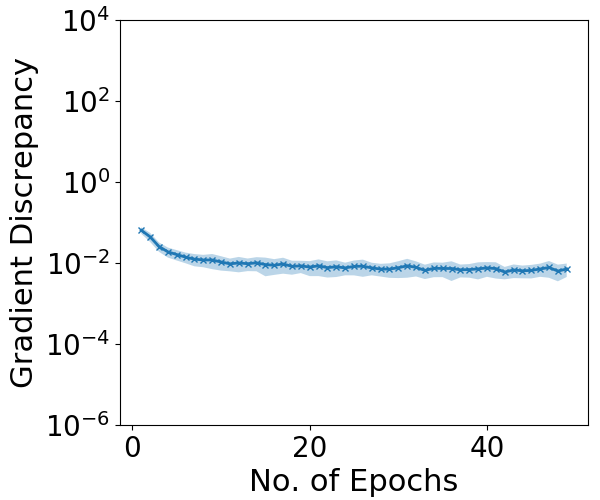
(a) Estimates of $\Delta_{t}^{2}(\bar{S}_{n+1})$

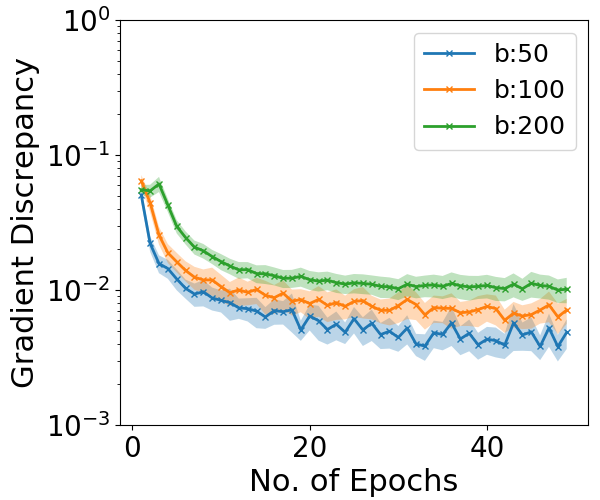
(b) Effect of batch size

Figure 5: Results for training CNN using SGLD on MNIST. (a) Estimation of $\Delta_{t}^{2}(\bar{S}_{n+1})$ using re-sampled $(S_{n},z_{n+1})$. The variance of such estimation is small. (b) The gradient discrepancy for different batch sizes. Overall, the differences are not significant.

Dependence of the bound on batchsize $b$. Our bound in Theorem 2 does not have a dependence on $b$, because of what Remark 3.2 shows, i.e., the $1/b$ scale factor neutralizes the leading b term in Lemma 1. The gradient discrepancy term itself may have a mild dependence on $b$, with smaller batch sizes having mildly smaller empirical gradient discrepancy as shown in Figure 5 (b).

Table 3: Details of Experiments reported in Figure 1 and 6 for MNIST and Fashion-MNIST with CNN

Parameter	Values
Dataset	MNIST/ Fashion-MNIST
Architecture	CNN with 2 conv. layers and 2 linear layers
Batch Size	$100$
Learning Rate	$\eta_{0}=4\times 10^{-3}$, decay epochs=5, decay rate=0.96
Inverse Temperature	$\beta\in[5000,55000]$
Number of Epochs	50
No. of training examples	55000
Number of Repeated Runs	30

Table 4: Details of Experiments reported in Figure 1 and 7 for CIFAR-10 with CNN

Parameter	Values
Dataset	CIFAR-10
Architecture	CNN with 2 conv. layers and 3 linear layers
Batch Size	$200$
Learning Rate	$\eta_{0}=5\times 10^{-3}$, decay epochs=5, decay rate=0.995
Inverse Temperature	$\beta\in[5000,55000]$
Number of Epochs	1000
No. of training examples	55000
Number of Repeated Runs	20

Table 5: Details of Experiments reported in Figure 3 for MNIST with CNN ($\sigma_{t}=0.2\cdot\eta_{t}$)

Parameter	Values
Dataset	MNIST
Architecture	CNN with 2 conv. layers and 2 linear layers
Batch Size	$100$
Learning Rate	$\eta_{0}=5\times 10^{-3}$, decay epochs=30, decay rate=0.995
Number of Epochs	1000
No. of training examples	10000
Number of Repeated Runs	30

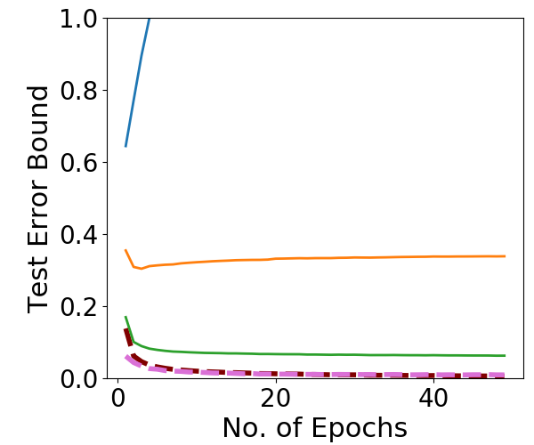
(a) MNIST, $\alpha_{t}^{2}\approx 0.1$, $\beta_{t}=55000$

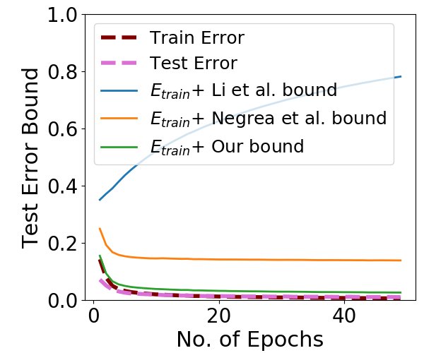
(b) MNIST, $\alpha_{t}^{2}\approx 0.1$, $\beta_{t}=5000$

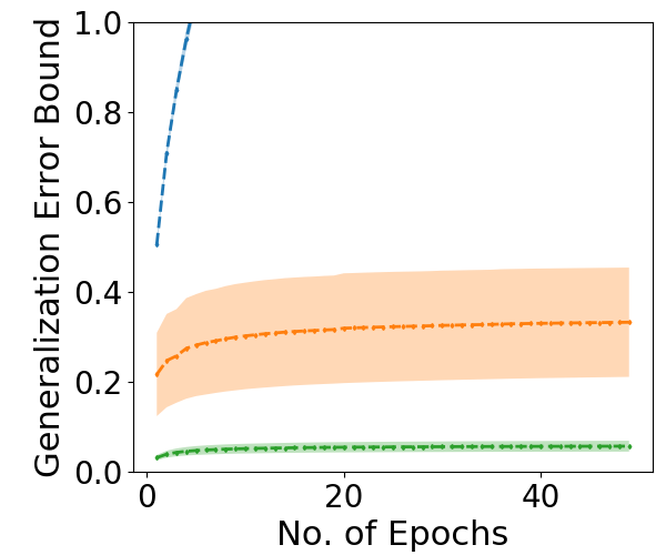
(c) MNIST, $\alpha_{t}^{2}\approx 0.1$, $\beta_{t}=55000$

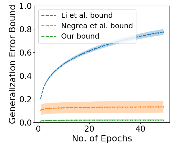
(d) MNIST, $\alpha_{t}^{2}\approx 0.1$, $\beta_{t}=5000$

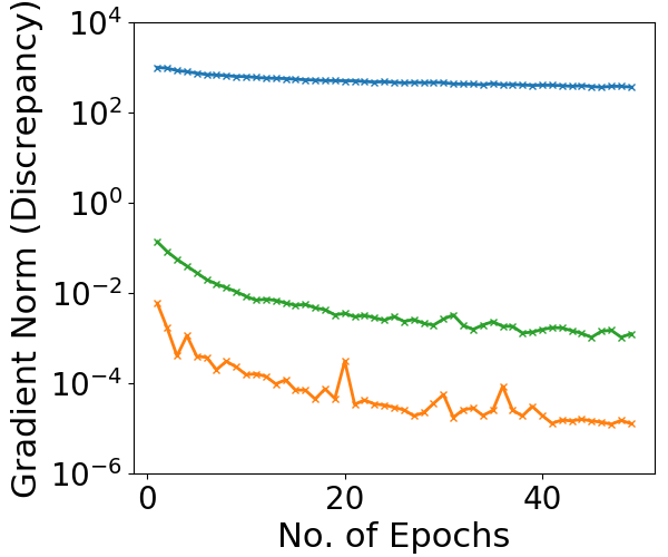
(e) MNIST, $\alpha_{t}^{2}\approx 0.1$, $\beta_{t}=55000$

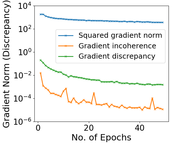
(f) MNIST, $\alpha_{t}^{2}\approx 0.1$, $\beta_{t}=5000$

Figure 6: Numerical results for CNN trained on MNIST using SGLD with a small noise variance $\sigma_{t}\approx 10^{-4}$.

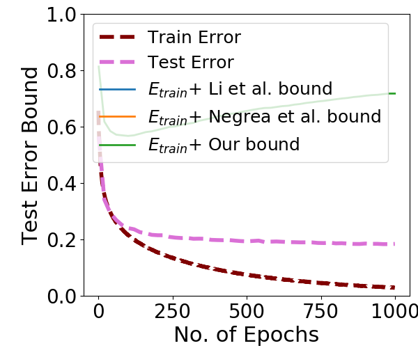
(a) CIFAR-10, $\alpha_{t}^{2}\approx 0.01$, $\beta_{t}=55000$

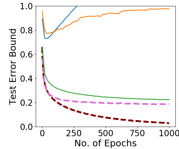
(b) CIFAR-10, $\alpha_{t}^{2}\approx 0.1$, $\beta_{t}=5000$

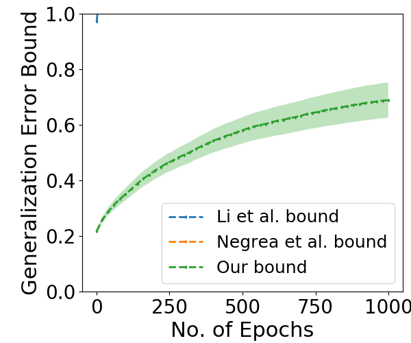
(c) CIFAR-10, $\alpha_{t}^{2}\approx 0.01$, $\beta_{t}=55000$

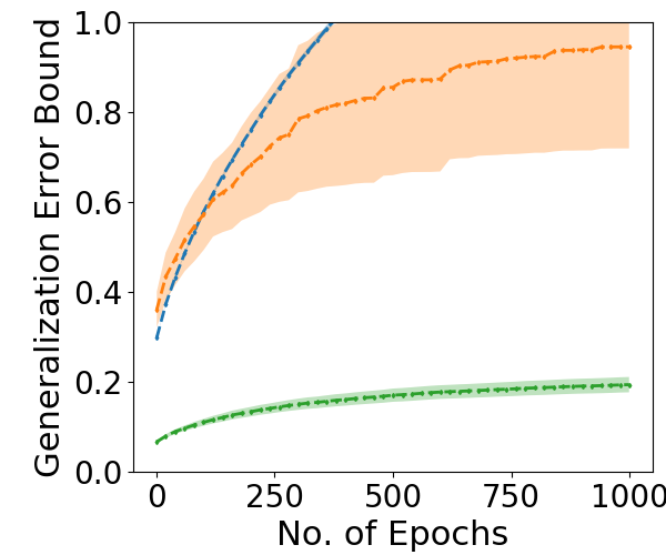
(d) CIFAR-10, $\alpha_{t}^{2}\approx 0.1$, $\beta_{t}=5000$

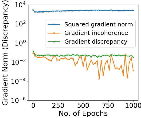
(e) CIFAR-10, $\alpha_{t}^{2}\approx 0.01$, $\beta_{t}=55000$

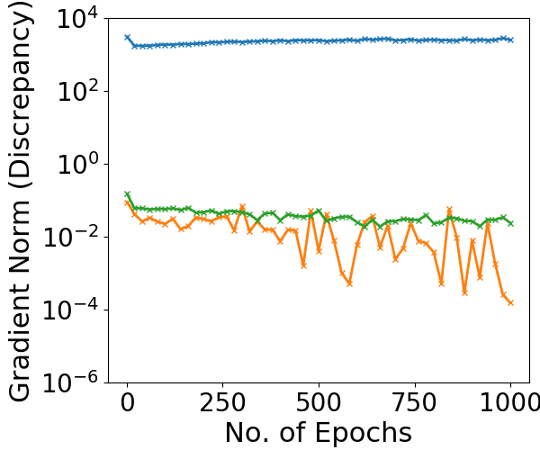
(f) CIFAR-10, $\alpha_{t}^{2}\approx 0.1$, $\beta_{t}=5000$

Figure 7: Numerical results for training CNN using SGLD on CIFAR-10.

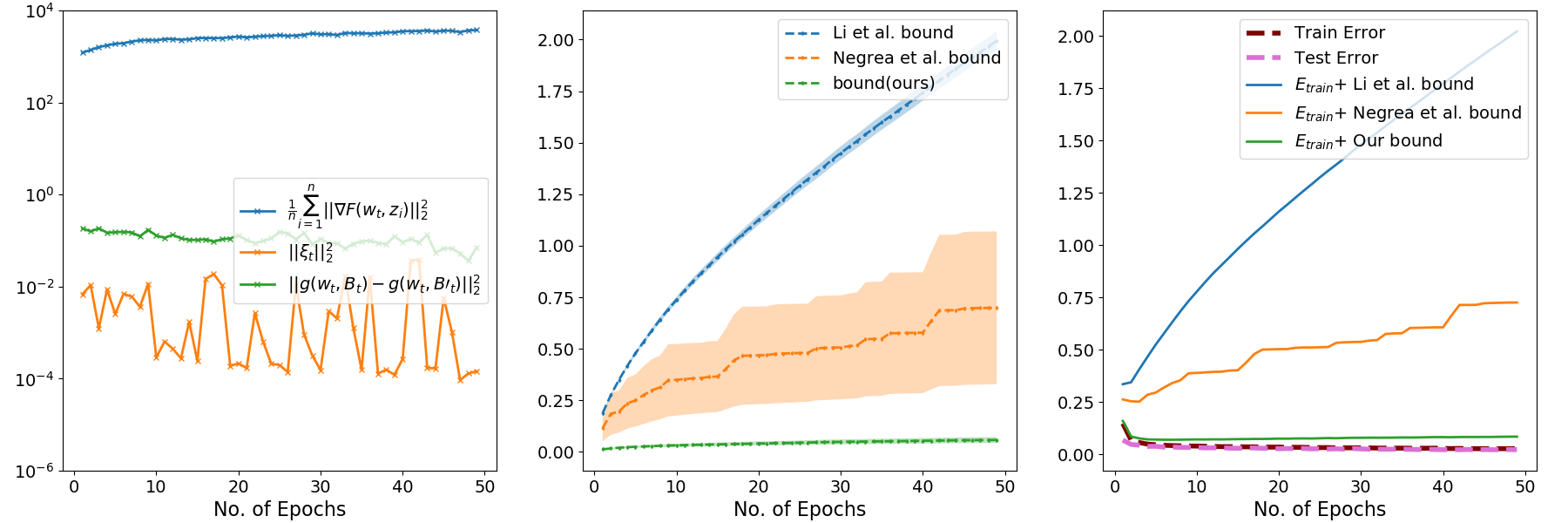
(a) CNN, MNIST, Noisy-SGD, $\alpha_{t}=0.2$, $\sigma_{t}\approx 10^{-4}$

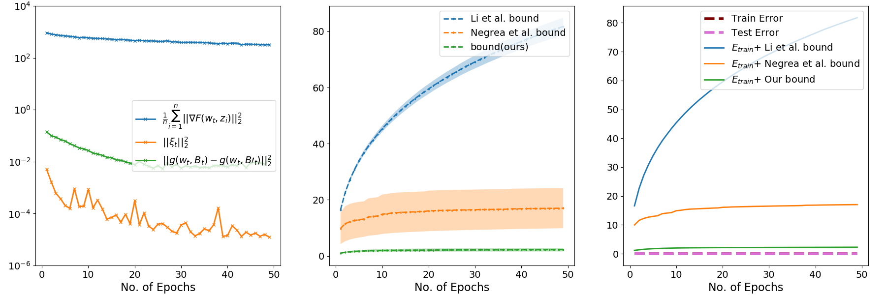
(b) CNN, MNIST, Noisy-SGD, $\alpha_{t}=0.002$, $\sigma_{t}\approx 10^{-6}$

Figure 8: Numerical results for CNN trained on MNIST using Noisy SGD. We follow the setting described in Li et al., (2020). The initial $\eta_{t}$ is $4\times 10^{-3}$, and decays by 0.95 ($\alpha_{t}=0.2$) or 0.995 ($\alpha_{t}=0.002$) for every 5 epochs.

(a) CNN, MNIST

(b) CNN, Fashion

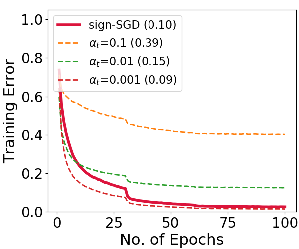
(c) ResNet-18, CIFAR10

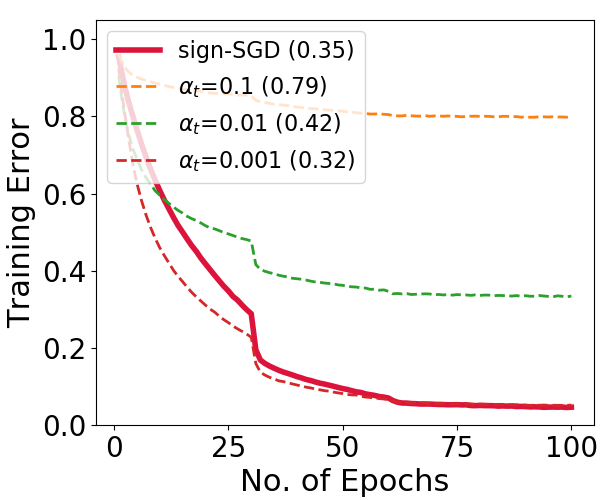
(d) ResNet-18, CIFAR100

Figure 9: Training dynamics of CNN on MNIST and Fashion-MNIST, and ResNet-18 on CIFAR-10 and CIFAR-100 using noisy sign-SGD with different scaling $\alpha_{t}$. Legends indicate the choice of $\alpha_{t}$ and the numbers in brackets are test errors at convergence. As $\alpha_{t}\to 0$, Nosiy sign-SGD matches both the optimization trajectory as well as the final test accuracy of the original sign-SGD (Bernstein et al., 2018a, ).

(a) MNIST, $\alpha_{t}=1.0$

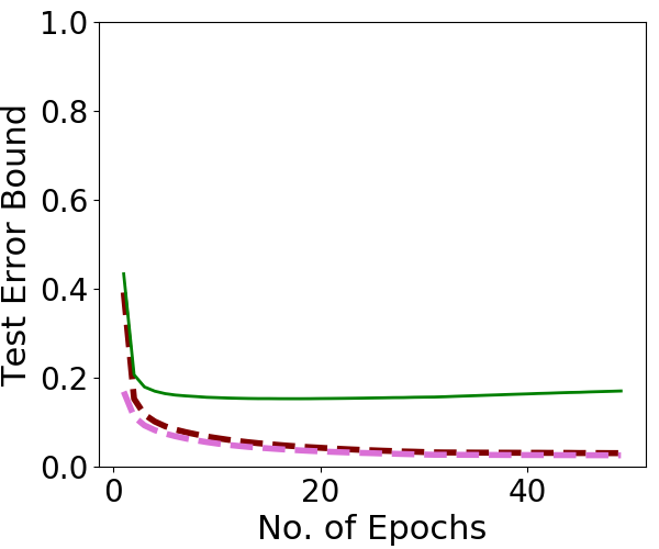
(b) MNIST, $\alpha_{t}=0.1$

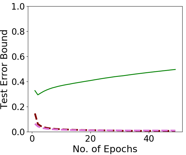
(c) MNIST, $\alpha_{t}=0.01$

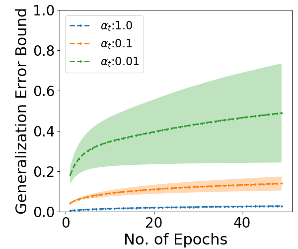
(d) MNIST, Our Bound

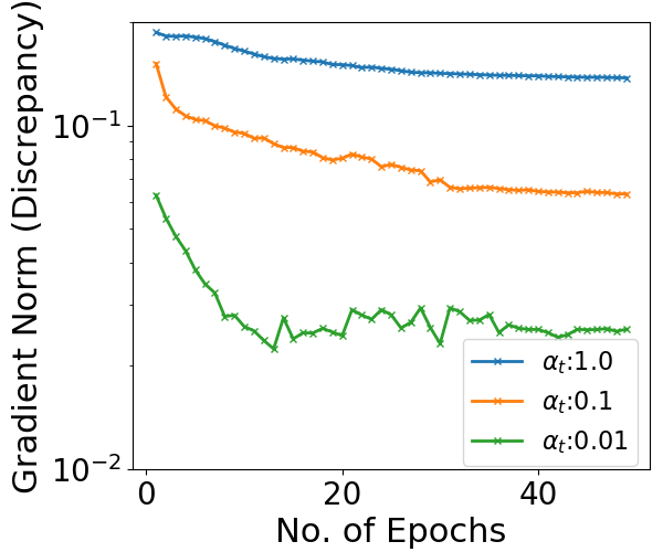
(e) MNIST, Gradient Discrepancy

(f) Fashion, $\alpha_{t}=1.0$

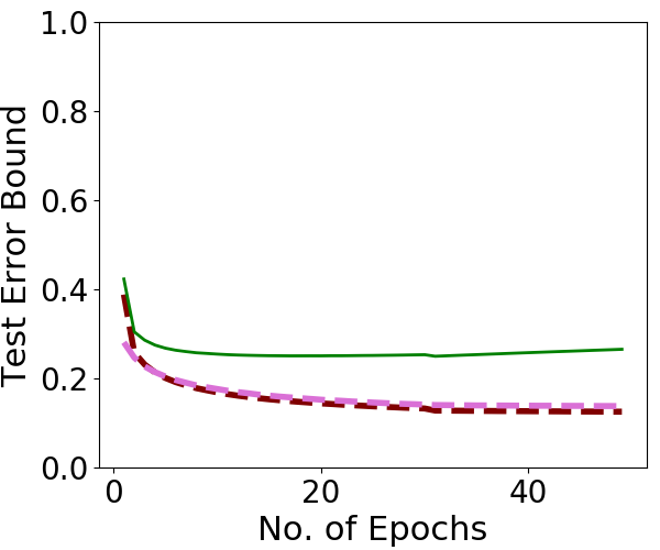
(g) Fashion, $\alpha_{t}=0.1$

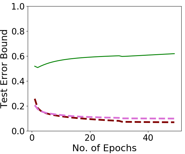
(h) Fashion, $\alpha_{t}=0.01$

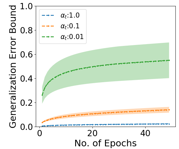
(i) Fashion, Our Bound

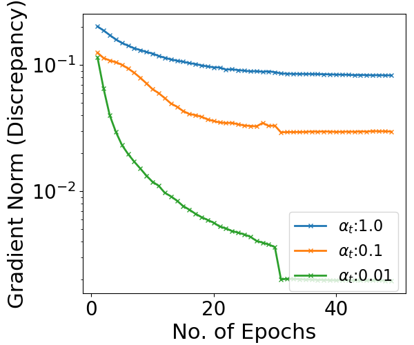
(j) Fashion, Gradient Discrepancy

Figure 10: Numerical results for training CNN on MNIST and Fashion-MNIST using Noisy Sign-SGD. Increasing $\alpha_{t}$ leads to a tighter generalization bound even though it leads to a slightly larger gradient discrepancy.

References

- Alistarh et al., (2017) Alistarh, D., Grubic, D., Li, J., Tomioka, R., and Vojnovic, M. (2017). Qsgd: Communication-efficient sgd via gradient quantization and encoding. In Guyon, I., Luxburg, U. V., Bengio, S., Wallach, H., Fergus, R., Vishwanathan, S., and Garnett, R., editors, Advances in Neural Information Processing Systems 30, pages 1709–1720. Curran Associates, Inc.
- Asi et al., (2021) Asi, H., Duchi, J., Fallah, A., Javidbakht, O., and Talwar, K. (2021). Private adaptive gradient methods for convex optimization. In International Conference on Machine Learning, pages 383–392. PMLR.
- Banerjee et al., (2005) Banerjee, A., Merugu, S., Dhillon, I. S., and Ghosh, J. (2005). Clustering with bregman divergences. Journal of machine learning research, 6(10).
- Barndorff-Nielsen, (2014) Barndorff-Nielsen, O. (2014). Information and exponential families: in statistical theory. John Wiley & Sons.
- Bassily et al., (2020) Bassily, R., Feldman, V., Guzmán, C., and Talwar, K. (2020). Stability of stochastic gradient descent on nonsmooth convex losses. Advances in Neural Information Processing Systems, 33.
- Bassily et al., (2019) Bassily, R., Feldman, V., Talwar, K., and Guha Thakurta, A. (2019). Private stochastic convex optimization with optimal rates. Advances in neural information processing systems.
- Bassily et al., (2014) Bassily, R., Smith, A., and Thakurta, A. (2014). Private empirical risk minimization: Efficient algorithms and tight error bounds. In 2014 IEEE 55th Annual Symposium on Foundations of Computer Science, pages 464–473. IEEE.
- (8) Bernstein, J., Wang, Y.-X., Azizzadenesheli, K., and Anandkumar, A. (2018a). signsgd: Compressed optimisation for non-convex problems. In International Conference on Machine Learning, pages 560–569. PMLR.
- (9) Bernstein, J., Zhao, J., Azizzadenesheli, K., and Anandkumar, A. (2018b). signsgd with majority vote is communication efficient and fault tolerant. In International Conference on Learning Representations.
- Boucheron et al., (2013) Boucheron, S., Lugosi, G., and Massart, P. (2013). Concentration inequalities: A nonasymptotic theory of independence. Oxford university press.
- Bousquet and Elisseeff, (2002) Bousquet, O. and Elisseeff, A. (2002). Stability and generalization. Journal of Machine Learning Research, 2:499–526.
- Bousquet et al., (2020) Bousquet, O., Klochkov, Y., and Zhivotovskiy, N. (2020). Sharper bounds for uniformly stable algorithms. In Conference on Learning Theory, pages 610–626. PMLR.
- Brown, (1986) Brown, L. D. (1986). Fundamentals of statistical exponential families: with applications in statistical decision theory. Ims.
- Bu et al., (2019) Bu, Y., Zou, S., and Veeravalli, V. V. (2019). Tightening mutual information based bounds on generalization error. In 2019 IEEE International Symposium on Information Theory (ISIT), pages 587–591. IEEE.
- Bun et al., (2018) Bun, M., Dwork, C., Rothblum, G. N., and Steinke, T. (2018). Composable and versatile privacy via truncated cdp. In Proceedings of the 50th Annual ACM SIGACT Symposium on Theory of Computing, pages 74–86.
- Canonne et al., (2020) Canonne, C. L., Kamath, G., and Steinke, T. (2020). The discrete gaussian for differential privacy. In NeurIPS.
- Chen et al., (2019) Chen, X., Chen, T., Sun, H., Wu, Z. S., and Hong, M. (2019). Distributed training with heterogeneous data: Bridging median-and mean-based algorithms. arXiv preprint arXiv:1906.01736.
- Damian et al., (2021) Damian, A., Ma, T., and Lee, J. (2021). Label noise sgd provably prefers flat global minimizers. arXiv preprint arXiv:2106.06530.
- Devroye and Wagner, (1979) Devroye, L. and Wagner, T. (1979). Distribution-free inequalities for the deleted and holdout error estimates. IEEE Transactions on Information Theory, 25(2):202–207.
- Elisseeff et al., (2005) Elisseeff, A., Evgeniou, T., Pontil, M., and Kaelbing, L. P. (2005). Stability of randomized learning algorithms. Journal of Machine Learning Research, 6(1).
- Farghly and Rebeschini, (2021) Farghly, T. and Rebeschini, P. (2021). Time-independent generalization bounds for SGLD in non-convex settings. In Beygelzimer, A., Dauphin, Y., Liang, P., and Vaughan, J. W., editors, Advances in Neural Information Processing Systems.
- Feldman and Vondrak, (2018) Feldman, V. and Vondrak, J. (2018). Generalization bounds for uniformly stable algorithms. In Proceedings of the 32nd International Conference on Neural Information Processing Systems, pages 9770–9780.
- Feldman and Vondrak, (2019) Feldman, V. and Vondrak, J. (2019). High probability generalization bounds for uniformly stable algorithms with nearly optimal rate. In Conference on Learning Theory, pages 1270–1279. PMLR.
- Grünwald et al., (2021) Grünwald, P., Steinke, T., and Zakynthinou, L. (2021). Pac-bayes, mac-bayes and conditional mutual information: Fast rate bounds that handle general vc classes. arXiv preprint arXiv:2106.09683.
- Haghifam et al., (2020) Haghifam, M., Negrea, J., Khisti, A., Roy, D. M., and Dziugaite, G. K. (2020). Sharpened generalization bounds based on conditional mutual information and an application to noisy, iterative algorithms. Advances in Neural Information Processing Systems.
- Hardt et al., (2016) Hardt, M., Recht, B., and Singer, Y. (2016). Train faster, generalize better: Stability of stochastic gradient descent. In International Conference on Machine Learning, pages 1225–1234.
- Hellström and Durisi, (2020) Hellström, F. and Durisi, G. (2020). Generalization bounds via information density and conditional information density. IEEE Journal on Selected Areas in Information Theory, 1(3):824–839.
- Hellström and Durisi, (2021) Hellström, F. and Durisi, G. (2021). Fast-rate loss bounds via conditional information measures with applications to neural networks. In 2021 IEEE International Symposium on Information Theory (ISIT), pages 952–957. IEEE.
- Jiang and Agrawal, (2018) Jiang, P. and Agrawal, G. (2018). A linear speedup analysis of distributed deep learning with sparse and quantized communication. In Bengio, S., Wallach, H., Larochelle, H., Grauman, K., Cesa-Bianchi, N., and Garnett, R., editors, Advances in Neural Information Processing Systems 31, pages 2525–2536. Curran Associates, Inc.
- Jin et al., (2017) Jin, C., Ge, R., Netrapalli, P., Kakade, S. M., and Jordan, M. I. (2017). How to escape saddle points efficiently. In International Conference on Machine Learning, pages 1724–1732.
- Jin et al., (2019) Jin, C., Netrapalli, P., Ge, R., Kakade, S. M., and Jordan, M. I. (2019). On nonconvex optimization for machine learning: Gradients, stochasticity, and saddle points. arXiv preprint arXiv:1902.04811.
- Jin et al., (2020) Jin, R., Huang, Y., He, X., Wu, T., and Dai, H. (2020). Stochastic-sign sgd for federated learning with theoretical guarantees. arXiv preprint arXiv:2002.10940.
- Kairouz et al., (2020) Kairouz, P., Ribero, M., Rush, K., and Thakurta, A. (2020). Dimension independence in unconstrained private erm via adaptive preconditioning. arXiv preprint arXiv:2008.06570.
- Krizhevsky, (2009) Krizhevsky, A. (2009). Learning Multiple Layers of Features from Tiny Images. Technical Report Vol. 1. No. 4., University of Toronto.
- LeCun et al., (1998) LeCun, Y., Bottou, L., Bengio, Y., and Haffner, P. (1998). Gradient-based learning applied to document recognition. Proceedings of the IEEE, 86(11):2278–2324.
- Lei and Ying, (2020) Lei, Y. and Ying, Y. (2020). Fine-grained analysis of stability and generalization for stochastic gradient descent. In International Conference on Machine Learning.
- Li et al., (2019) Li, B., Chen, C., Liu, H., and Carin, L. (2019). On connecting stochastic gradient mcmc and differential privacy. In The 22nd International Conference on Artificial Intelligence and Statistics, pages 557–566. PMLR.
- Li et al., (2020) Li, J., Luo, X., and Qiao, M. (2020). On generalization error bounds of noisy gradient methods for non-convex learning. In International Conference on Learning Representations.
- Mou et al., (2018) Mou, W., Wang, L., Zhai, X., and Zheng, K. (2018). Generalization bounds of sgld for non-convex learning: Two theoretical viewpoints. In Conference on Learning Theory, pages 605–638. PMLR.
- Negrea et al., (2019) Negrea, J., Haghifam, M., Dziugaite, G. K., Khisti, A., and Roy, D. M. (2019). Information-theoretic generalization bounds for sgld via data-dependent estimates. In Advances in Neural Information Processing Systems.
- Neu et al., (2021) Neu, G., Dziugaite, G. K., Haghifam, M., and Roy, D. M. (2021). Information-theoretic generalization bounds for stochastic gradient descent. In COLT.
- Pensia et al., (2018) Pensia, A., Jog, V., and Loh, P.-L. (2018). Generalization error bounds for noisy, iterative algorithms. In 2018 IEEE International Symposium on Information Theory (ISIT), pages 546–550. IEEE.
- Pollard, (2002) Pollard, D. (2002). A user’s guide to measure theoretic probability. Number 8. Cambridge University Press.
- Raginsky et al., (2017) Raginsky, M., Rakhlin, A., and Telgarsky, M. (2017). Non-convex learning via stochastic gradient langevin dynamics: a nonasymptotic analysis. In Conference on Learning Theory, pages 1674–1703. PMLR.
- Rodríguez-Gálvez et al., (2021) Rodríguez-Gálvez, B., Bassi, G., Thobaben, R., and Skoglund, M. (2021). On random subset generalization error bounds and the stochastic gradient langevin dynamics algorithm. In 2020 IEEE Information Theory Workshop (ITW), pages 1–5. IEEE.
- Rogers and Wagner, (1978) Rogers, W. H. and Wagner, T. J. (1978). A finite sample distribution-free performance bound for local discrimination rules. The Annals of Statistics, pages 506–514.
- Russo and Zou, (2016) Russo, D. and Zou, J. (2016). Controlling bias in adaptive data analysis using information theory. In Artificial Intelligence and Statistics, pages 1232–1240. PMLR.
- Sason and Verdu, (2016) Sason, I. and Verdu, S. (2016). -divergence inequalities. IEEE Transactions on Information Theory, 62.
- Shalev-Shwartz et al., (2009) Shalev-Shwartz, S., Shamir, O., Srebro, N., and Sridharan, K. (2009). Stochastic convex optimization. In COLT.
- Shamir and Zhang, (2013) Shamir, O. and Zhang, T. (2013). Stochastic gradient descent for non-smooth optimization: Convergence results and optimal averaging schemes. In International conference on machine learning, pages 71–79. PMLR.
- Steinke and Zakynthinou, (2020) Steinke, T. and Zakynthinou, L. (2020). Reasoning about generalization via conditional mutual information. In Conference on Learning Theory, pages 3437–3452. PMLR.
- Tsybakov, (2008) Tsybakov, A. B. (2008). Introduction to nonparametric estimation. Springer Science & Business Media.
- Wainwright and Jordan, (2008) Wainwright, M. J. and Jordan, M. I. (2008). Graphical models, exponential families, and variational inference. Now Publishers Inc.
- (54) Wang, B., Zhang, H., Zhang, J., Meng, Q., Chen, W., and Liu, T.-Y. (2021a). Optimizing information-theoretical generalization bound via anisotropic noise of SGLD. In Beygelzimer, A., Dauphin, Y., Liang, P., and Vaughan, J. W., editors, Advances in Neural Information Processing Systems.
- Wang and Xu, (2019) Wang, D. and Xu, J. (2019). Differentially private empirical risk minimization with smooth non-convex loss functions: A non-stationary view. In Proceedings of the AAAI Conference on Artificial Intelligence, volume 33, pages 1182–1189.
- (56) Wang, H., Huang, Y., Gao, R., and Calmon, F. (2021b). Analyzing the generalization capability of sgld using properties of gaussian channels. Advances in Neural Information Processing Systems, 34.
- Wang et al., (2015) Wang, Y.-X., Fienberg, S., and Smola, A. (2015). Privacy for free: Posterior sampling and stochastic gradient monte carlo. In International Conference on Machine Learning, pages 2493–2502. PMLR.
- Welling and Teh, (2011) Welling, M. and Teh, Y. W. (2011). Bayesian learning via stochastic gradient langevin dynamics. In International Conference on Machine Learning, ICML ’11, pages 681–688.
- Xiao et al., (2017) Xiao, H., Rasul, K., and Vollgraf, R. (2017). Fashion-mnist: a novel image dataset for benchmarking machine learning algorithms.
- Xu and Raginsky, (2017) Xu, A. and Raginsky, M. (2017). Information-theoretic analysis of generalization capability of learning algorithms. Advances in Neural Information Processing Systems, 2017:2525–2534.
- Yang et al., (2019) Yang, G., Zhang, T., Kirichenko, P., Bai, J., Wilson, A. G., and De Sa, C. (2019). Swalp: Stochastic weight averaging in low-precision training. 36th International Conference on Machine Learning (ICML).
- Zhang et al., (2017) Zhang, C., Bengio, S., Hardt, M., Recht, B., and Vinyals, O. (2017). Understanding deep learning requires rethinking generalization. In 5th International Conference on Learning Representations, ICLR 2017, Toulon, France, April 24-26, 2017, Conference Track Proceedings. OpenReview.net.
- Zhang et al., (2021) Zhang, H., Mironov, I., and Hejazinia, M. (2021). Wide network learning with differential privacy. arXiv preprint arXiv:2103.01294.
- Zhou et al., (2021) Zhou, R., Tian, C., and Liu, T. (2021). Individually conditional individual mutual information bound on generalization error. In 2021 IEEE International Symposium on Information Theory (ISIT), pages 670–675. IEEE.
- Zhou et al., (2020) Zhou, Y., Wu, S., and Banerjee, A. (2020). Bypassing the ambient dimension: Private sgd with gradient subspace identification. In International Conference on Learning Representations.