Hadronic molecule model for the doubly charmed state $T^{+}_{cc}$

Abstract

The mass, current coupling, and width of the doubly charmed four-quark meson $T_{cc}^{+}$ are explored by treating it as a hadronic molecule $M_{cc}^{+}\equiv D^{0}D^{\ast+}$. The mass and current coupling of this molecule are calculated using the QCD two-point sum rule method by including into analysis contributions of various vacuum condensates up to dimension $10$. The prediction for the mass $m=(4060\pm 130)~{}\mathrm{MeV}$ exceeds the two-meson $D^{0}D^{\ast+}$ threshold $3875.1~{}\mathrm{MeV}$, which makes decay of the molecule $M_{cc}^{+}$ to a pair of conventional mesons $D^{0}D^{\ast+}$ kinematically allowed process. The strong coupling $G$ of particles at the vertex $M_{cc}^{+}D^{0}D^{\ast+}$ is found by applying the QCD three-point sum rule approach, and used to evaluate the width of the decay $M_{cc}^{+}\to D^{0}D^{\ast+}$. Obtained result for the width $\Gamma=(3.8\pm 1.7)~{}\mathrm{MeV}$ demonstrates that $M_{cc}^{+}$ is wider than the resonance $T_{cc}^{+}$.

I Introduction

Recently, the LHCb collaboration informed about observation, for the first time, of a doubly charmed axial-vector state $T_{cc}^{+}$  composed of four quarks $cc\overline{u}\overline{d}$ Aaij:2021vvq ; LHCb:2021auc . This state was fixed in $D^{0}D^{0}\pi^{+}$ mass distribution as a narrow peak with the width $\Gamma=(410\pm 165\pm 43_{-38}^{+18})~{}\mathrm{keV}$, which means that it is longest living exotic meson discovered till now. The mass of $T_{cc}^{+}$ is very close to the two-meson $D^{0}D^{\ast+}$ threshold $3875.1~{}\mathrm{MeV}$, but is smaller than this limit by an amount of $\delta m_{\exp}=(-273\pm 61\pm 5_{-14}^{+11})~{}\mathrm{keV}$. These features of $T_{cc}^{+}$, in particular its narrow width, made the doubly charmed exotic meson $T_{cc}^{+}$ an object of intensive studies Agaev:2021vur ; Feijoo:2021ppq ; Yan:2021wdl ; Fleming:2021wmk ; Azizi:2021aib ; Meng:2021jnw ; Ling:2021bir ; Chen:2021vhg ; Xin:2021wcr .

It is worth emphasizing that doubly charmed tetraquarks attracted already interests of researchers. This is connected with estimated stability some of tetraquarks containing heavy diquarks $bb$, $bc$ and $cc$ against strong and maybe electromagnetic decays. If exist, such particles can transform to mesons only through weak decays, and have mean lifetimes which would be considerably longer than that of conventional mesons Agaev:2018khe ; Agaev:2019lwh ; Agaev:2020zag ; Agaev:2019kkz . There is growing conviction that tetraquarks built of $bb$ diquarks are stable particles, whereas the situation with ones composed of $bc$ and $cc$ diquarks is still remaining controversial Karliner:2017qjm ; Eichten:2017ffp ; Agaev:2020zad .

Because the present work is devoted to investigation of doubly charmed states, below we restrict ourselves by analyses of problems and achievements connected only with these particles. Thus, tetraquarks $cc\overline{q}\overline{q}^{\prime}$ were theoretically studied using different methods of the high energy physics. In the framework of the QCD sum rule method they were analyzed in Refs. Navarra:2007yw ; Du:2012wp . In the first article the authors explored the axial-vector tetraquark $cc\overline{u}\overline{d}$. Prediction for its mass $(4000\pm 200)~{}\mathrm{MeV}$ implies that the axial-vector tetraquark $cc\overline{u}\overline{d}$ is unstable and readily decays to mesons $D^{0}D^{\ast}{}^{+}$. Four-quark exotic mesons of general $cc\overline{q}\overline{q}^{\prime}$ content and quantum numbers $J^{\mathrm{P}}=0^{-},~{}0^{+},~{}1^{-}$ and $1^{+}$ were investigated in Ref. Du:2012wp . In accordance with results of this analysis, masses of tetraquarks $cc\overline{q}\overline{q}$, $cc\overline{q}\overline{s}$, and $cc\overline{s}\overline{s}$ are above corresponding thresholds for all explored quantum numbers. In other words, a class of tetraquarks composed of a diquark $cc$ and a light antidiquark does not contain strong-interaction stable particles.

Discovery of doubly charmed baryon $\Xi_{cc}^{++}=ccu$ by the LHCb collaboration Aaij:2017ueg , and extracted experimental information stimulated relatively new studies of heavy tetraquarks. A reason was that, these experimental data were employed as new input parameters in a phenomenological model to estimate masses of the axial-vector tetraquarks $T_{bb;\overline{u}\overline{d}}^{-}$ and $T_{cc;\overline{u}\overline{d}}^{+}$ Karliner:2017qjm ; Eichten:2017ffp . In these articles it was demonstrated that $T_{cc;\overline{u}\overline{d}}^{+}$ has the mass $(3882\pm 12)~{}\mathrm{MeV}$ and $3978~{}\mathrm{MeV}$, respectively, which are above thresholds for both $D^{0}D^{\ast+}$ and $D^{0}D^{+}\gamma$ decays. Other members of $cc\overline{q}\overline{q}$, and $cc\overline{q}\overline{s}$ families were considered in Ref. Eichten:2017ffp : None of them were classified as a stable state. Similar conclusions about properties of $T_{cc;\overline{u}\overline{d}}^{+}$ were drawn in Refs. Wang:2017dtg ; Braaten:2020nwp ; Cheng:2020wxa as well. Contrary to these studies, in Ref. Meng:2020knc the authors calculated the mass of $T_{cc;\overline{u}\overline{d}}^{+}$ using a constituent quark model and found that it is $23~{}\mathrm{MeV}$ below the two-meson threshold. Stable nature of $T_{cc;\overline{u}\overline{d}}^{+}$ was demonstrated also by means of lattice simulations Junnarkar:2018twb , in which its mass was estimated $(-23\pm 11)~{}\mathrm{MeV}$ below the two-meson threshold.

Detailed studies of pseudoscalar and scalar exotic mesons $cc\overline{u}\overline{d}$ were done in Ref. Agaev:2019qqn . Analysis performed there, demonstrated that these particles are strong-interaction unstable structures, and fall apart to conventional mesons. Full widths of these tetraquarks were evaluated by utilizing their decays to $D^{+}D^{\ast}(2007)^{0}$, $D^{0}D^{\ast}(2010)^{+}$, and $D^{0}D^{+}$ mesons, respectively. It was found, that these structures with widths $\sim 130~{}\mathrm{MeV}$ and $\sim 12~{}\mathrm{MeV}$ are relatively wide resonances. Structures $cc\overline{s}\overline{s}$ and $cc\overline{d}\overline{s}$ form another interesting subgroup of doubly charmed tetraquarks, because they are also doubly charged particles. Masses and widths of such pseudoscalar tetraquarks were evaluated in Ref. Agaev:2018vag .

Doubly charmed four-quark structures were studied also in the context of the hadronic molecule picture, i.e., they were modeled as molecules of conventional mesons. It is worth noting that charmonium molecules are not new objects for investigations: Problems of such compounds were addressed in literature decades ago Novikov:1977dq . As a hadronic molecule $M_{cc}^{+}\equiv D^{0}D^{\ast+}$ built of ordinary mesons $D^{0}$ and $D^{\ast+}$, the axial-vector state $cc\overline{u}\overline{d}$ was considered in Refs. Dias:2011mi ; Li:2012ss . The mass of $M_{cc}^{+}$ was estimated in Ref. Dias:2011mi using the QCD spectral sum rule approach. Obtained prediction $(3872.2\pm 39.5)~{}\mathrm{MeV}$ shows that this molecule cannot decay to mesons $D^{0}$ and $D^{\ast+}$, but its mass is enough to trigger the strong decay $M_{cc}^{+}\rightarrow D^{0}D^{0}\pi^{+}$.

In our recent article, we treated $T_{cc}^{+}$ as an axial-vector diquark-antidiquark (tetraquark) state with quark content $cc\overline{u}\overline{d}$, and calculated its spectroscopic parameters and full width Agaev:2021vur . Computations performed in the context of the QCD two-point sum rule method led for the mass of this state to the result $(3868\pm 124)~{}\mathrm{MeV}$, which is consistent with the LHCb measurements. This means that $T_{cc}^{+}$ does not decay to a meson pair $D^{0}D^{\ast+}$. Therefore, we evaluated full width of $T_{cc}^{+}$ by considering its alternative strong decay channels. In fact, production of $D^{0}D^{0}\pi^{+}$ can run through decay of $T_{cc}^{+}$ to a scalar tetraquark $T_{cc;\overline{u}\overline{u}}^{0}$ and $\pi^{+}$ followed by the process $T_{cc;\overline{u}\overline{u}}^{0}\rightarrow D^{0}D^{0}$. The process $T_{cc}^{+}\rightarrow\widetilde{T}\pi^{0}\rightarrow D^{0}D^{+}\pi^{0}$ is another decay mode of $T_{cc}^{+}$. Here, $\widetilde{T}$  is the scalar exotic meson with content $cc\overline{u}\overline{d}$. This means, that in our analysis decays to scalar tetraquarks $T_{cc;\overline{u}\overline{u}}^{0}$ and $\widetilde{T}$  was considered as a dominant mechanism for transformation of $T_{cc}^{+}$ . Full width of $T_{cc}^{+}$ estimated in Ref. Agaev:2021vur equals to $\Gamma=(489\pm 92)~{}\mathrm{keV}$ which nicely agrees with the experimental data.

As is seen, an assumption about the diquark-antidiquark structure of $T_{cc}^{+}$ gives for its mass and width results compatible with the LHCb data Agaev:2021vur . In accordance to Ref. Dias:2011mi , the molecule model for the mass of $M_{cc}^{+}$ leads to almost the same prediction. Unfortunately, in this paper the authors did not compute width of the molecule $M_{cc}^{+}$, therefore it is difficult to declare a full convergence of results for $T_{cc}^{+}$ and $M_{cc}^{+}$ obtained in the framework of the QCD sum rule method. The reason is that masses of $T_{cc}^{+}$ and $M_{cc}^{+}$ were extracted, as usual, with theoretical uncertainties, and due to overlapping of relevant regions, this information is not enough to distinguish diquark-antidiquark and molecule states. To make reliable statements about internal organization of the four-quark state seen by LHCb, it is necessary to investigate decay modes of this particle, and calculate its full width.

The program outlined above was realized in the diquark-antidiquark picture in our article Agaev:2021vur . In the present work, we consider this problem in the framework of the hadronic molecule model, and calculate the mass and width of $M_{cc}^{+}$. We wish to answer a question whether both the mass and width of $M_{cc}^{+}$ agree with new LHCb data. For these purposes, we calculate the spectroscopic parameters of $M_{cc}^{+}$ using the QCD two-point sum rule method Shifman:1978bx ; Shifman:1978by . Our analysis proves that the mass of $M_{cc}^{+}$ exceeds the LHCb data, which makes the process $M_{cc}^{+}\rightarrow D^{0}D^{\ast+}$ kinematically allowed one. The width of this decay channel is found by means of the three-point version of QCD sum rule approach: It is used to extract the strong coupling $G$ at the vertex $M_{cc}^{+}D^{0}D^{\ast+}$.

This article is structured in the following manner: In Sec. II, we compute the mass $m$ and coupling $f$ of the molecule $M_{cc}^{+}$ in the context of the QCD two-point sum rule method. In these calculations, we take into account various vacuum condensates up to dimension $10$. In Sec. III, we consider the decay mode $M_{cc}^{+}\rightarrow D^{0}D^{\ast+}$, find the strong coupling $G$ and evaluate the width of this process. We reserve Sec. IV for discussion and conclusions.

II Spectroscopic parameters of $M_{cc}^{+}$

The sum rules necessary to evaluate the spectroscopic parameters of the molecule $M_{cc}^{+}$ can be derived from analysis of the correlation function

$$\Pi_{\mu\nu}(p)=i\int d^{4}xe^{ipx}\langle 0|\mathcal{T}\{J_{\mu}(x)J_{\nu}^{{\dagger}}(0)\}|0\rangle,$$ (1)

where $J_{\mu}(x)$ is the interpolation current for the axial-vector state $M_{cc}^{+}$. In the hadronic molecule model the current $J_{\mu}(x)$ is given by the expression

$$J_{\mu}(x)=\overline{d}_{a}(x)\gamma_{\mu}c_{a}(x)\overline{u}_{b}(x)\gamma_{5}c_{b}(x),$$ (2)

where $a$ and $b$ are color indices.

To find the sum rules for $m$ and $f$, we express the correlation function $\Pi_{\mu\nu}(p)$ in terms of $M_{cc}^{+}$ molecule’s physical parameters. Because $M_{cc}^{+}$ is composed of ground-state mesons $D^{0}$ and $D^{\ast+}$, it can be treated as lowest lying system in this class of particles. Therefore, in the correlation function $\Pi_{\mu\nu}^{\mathrm{Phys}}(p)$, we write down explicitly only first term that corresponds to $M_{cc}^{+}$

$$\Pi_{\mu\nu}^{\mathrm{Phys}}(p)=\frac{\langle 0|J_{\mu}|M_{cc}^{+}(p,\epsilon)\rangle\langle M_{cc}^{+}(p,\epsilon)|J_{\nu}^{\dagger}|0\rangle}{m^{2}-p^{2}}+\cdots.$$ (3)

The $\Pi_{\mu\nu}^{\mathrm{Phys}}(p)$ is obtained by inserting into the correlation function Eq. (1) the full set of states with spin-parities $J^{\mathrm{P}}=1^{+}$, and carrying out integration over $x$. The dots in Eq. (3) denote contributions coming from higher resonances and continuum states.

To derive Eq. (3), we assume that the physical side of the sum rule can be approximated by a single pole term. In the case of the multiquark systems $\Pi_{\mu\nu}^{\mathrm{Phys}}(p)$ receives contribution, however, also from two-meson reducible terms Kondo:2004cr ; Lee:2004xk . That is because the current $J_{\mu}(x)$ interacts not only with a molecule $M_{cc}^{+}$, but also with the two-meson continuum with the same quantum numbers and quark content. Effects of current-continuum interaction, properly taken into account, generates a finite width $\Gamma(p^{2})$ of the hadronic molecule and leads to the modification in Eq. (3) in accordance with the prescription Wang:2015nwa

$$\frac{1}{m^{2}-p^{2}}\rightarrow\frac{1}{m^{2}-p^{2}-i\sqrt{p^{2}}\Gamma(p^{2})}.$$ (4)

The two-meson contributions can be included into analysis by rescaling the coupling $f$ of $M_{cc}^{+}$, and keeping untouched its mass. Calculations demonstrated that these effects are small and do not exceed uncertainties of sum rule calculations. Indeed, in the case of the doubly charmed pseudoscalar tetraquark $cc\overline{s}\overline{s}$ with the mass $m_{T}=4390~{}\mathrm{MeV}$ and full width $\Gamma_{T}\approx 300~{}\mathrm{MeV}$, two-meson effects lead to additional $\approx 7\%$ uncertainty in the current coupling $f_{T}$ Agaev:2018vag . For the resonance $Z_{c}^{-}(4100)$ these ambiguities amount to $\approx 5\%$ of the coupling $f_{Z_{c}}$ Sundu:2018nxt . As we shall see below, the molecule $M_{cc}^{+}$ has the width $(3.8\pm 1.7)~{}\mathrm{MeV}$. Therefore, aforementioned effects are negligible, and in $\Pi_{\mu\nu}^{\mathrm{Phys}}(p)$ it is enough to employ the zero-width single-pole approximation.

The function $\Pi_{\mu\nu}^{\mathrm{Phys}}(p)$ can be presented in a more compact form. To this end, we introduce the matrix element

$$\langle 0|J_{\mu}|M_{cc}^{+}(p,\epsilon)\rangle=fm\epsilon_{\mu},$$ (5)

where $\epsilon_{\mu}$ is the polarization vector of the molecule $M_{cc}^{+}$. It is not difficult to demonstrate that the function $\Pi_{\mu\nu}^{\mathrm{Phys}}(p)$ in terms of $m$ and $f$  has the simple form

$$\Pi_{\mu\nu}^{\mathrm{Phys}}(p)=\frac{m^{2}f^{2}}{m^{2}-p^{2}}\left(-g_{\mu\nu}+\frac{p_{\mu}p_{\nu}}{m^{2}}\right)+\cdots.$$ (6)

The QCD side of the sum rules $\Pi_{\mu\nu}^{\mathrm{OPE}}(p)$ has to be calculated in the operator product expansion ($\mathrm{OPE}$) with some fixed accuracy. To find $\Pi_{\mu\nu}^{\mathrm{OPE}}(p)$, we calculate the correlation function using explicit form of the current $J_{\mu}(x)$. As a result, we express $\Pi_{\mu\nu}^{\mathrm{OPE}}(p)$ in terms of heavy and light quark propagators

$$\Pi_{\mu\nu}^{\mathrm{OPE}}(p)=i\int d^{4}xe^{ip\cdot x}\left\{\mathrm{Tr}\left[\gamma_{5}S_{c}^{bb^{\prime}}(x)\gamma_{5}S_{u}^{b^{\prime}b}(-x)\right]\right.$$

$$\times\mathrm{Tr}\left[\gamma_{\mu}S_{c}^{aa^{\prime}}(x)\gamma_{\nu}S_{d}^{a^{\prime}a}(-x)\right]-\mathrm{Tr}\left[\gamma_{\mu}S_{c}^{ab^{\prime}}(x)\gamma_{5}\right.$$

$$\left.\left.\times S_{u}^{b^{\prime}b}(-x)\gamma_{5}S_{c}^{ba^{\prime}}(x)\gamma_{\nu}S_{d}^{a^{\prime}a}(-x)\right]\right\}.$$ (7)

In Eq. (7) $S_{q}^{ab}(x)$ and $S_{c}^{ab}(x)$ are propagators of $q(u,d)$ and $c$-quarks, formulas for which are collected in Appendix.

The QCD sum rules can be derived using the same Lorentz structures in $\Pi_{\mu\nu}^{\mathrm{Phys}}(p)$ and $\Pi_{\mu\nu}^{\mathrm{OPE}}(p)$. For our purposes, the structures proportional to $g_{\mu\nu}$ are appropriate, because they are free of contributions of spin-$0$ particles. To obtain a sum rule, we equate invariant amplitudes $\Pi^{\mathrm{Phys}}(p^{2})$ and $\Pi^{\mathrm{OPE}}(p^{2})$ corresponding to these structures, and apply the Borel transformation to both sides of the obtained expression. The last operation is necessary to suppress contributions stemming from the higher resonances and continuum states. At the following phase of manipulations, we make use an assumption about the quark-hadron duality, and subtract from the physical side of the equality higher resonances’ and continuum contributions. By this way, the final sum rule equality acquires a dependence on the Borel $M^{2}$ and continuum threshold (subtraction) $s_{0}$ parameters. This equality, and second expression obtained by applying the operator $d/d(-1/M^{2})$ to its both sides, form a system which is used to find sum rules for the mass $m$ and coupling $f$

$$m^{2}=\frac{\Pi^{\prime}(M^{2},s_{0})}{\Pi(M^{2},s_{0})},$$ (8)

$$f^{2}=\frac{e^{m^{2}/M^{2}}}{m^{2}}\Pi(M^{2},s_{0}),$$ (9)

where $\Pi^{\prime}(M^{2},s_{0})=d\Pi(M^{2},s_{0})/d(-1/M^{2})$.

In Eqs. (8) and (9) the function $\Pi(M^{2},s_{0})$ is Borel transformed and continuum subtracted invariant amplitude $\Pi^{\mathrm{OPE}}(p^{2})$. We calculate $\Pi(M^{2},s_{0})$ by taking into account quark, gluon and mixed vacuum condensates up to dimension $10$. It has the following form

$$\Pi(M^{2},s_{0})=\int_{4m_{c}^{2}}^{s_{0}}ds\rho^{\mathrm{OPE}}(s)e^{-s/M^{2}}+\Pi(M^{2}),$$ (10)

where $\rho^{\mathrm{OPE}}(s)$ is the two-point spectral density. The second component of the invariant amplitude $\Pi(M^{2})$ contains nonperturbative contributions calculated directly from $\Pi_{\mu\nu}^{\mathrm{OPE}}(p)$. The explicit expression of the function $\Pi(M^{2},s_{0})$ is removed to Appendix.

The quark, gluon and mixed condensates which enter to the sum rules (8) and (9) are universal parameters of computations:

$$\langle\overline{q}q\rangle=-(0.24\pm 0.01)^{3}~{}\mathrm{GeV}^{3},\$$

$$\langle\overline{q}g_{s}\sigma Gq\rangle=m_{0}^{2}\langle\overline{q}q\rangle,\ m_{0}^{2}=(0.8\pm 0.1)~{}\mathrm{GeV}^{2},\$$

$$\langle\frac{\alpha_{s}G^{2}}{\pi}\rangle=(0.012\pm 0.004)~{}\mathrm{GeV}^{4},$$

$$\langle g_{s}^{3}G^{3}\rangle=(0.57\pm 0.29)~{}\mathrm{GeV}^{6},$$

$$m_{c}=1.275\pm 0.025~{}\mathrm{GeV}.$$ (11)

The correlation function $\Pi(M^{2},s_{0})$ depends on the $c$ quark mass, numerical value of which is shown in Eq. (11) as well. Contrary, the Borel and continuum threshold parameters $M^{2}$ and $s_{0}$ are auxiliary quantities of calculations: Their choice depends on the problem under consideration, and has to meet restrictions imposed on the pole contribution ($\mathrm{PC}$) and convergence of $\mathrm{OPE}$.

To estimate the $\mathrm{PC}$, we use the expression

$$\mathrm{PC}=\frac{\Pi(M^{2},s_{0})}{\Pi(M^{2},\infty)}.$$ (12)

The convergence of the operator product expansion is checked by means of the formula

$$R(M^{2})=\frac{\Pi^{\mathrm{DimN}}(M^{2},s_{0})}{\Pi(M^{2},s_{0})},$$ (13)

where $\Pi^{\mathrm{DimN}}(M^{2},s_{0})$ is the contribution of the last three terms in $\mathrm{OPE}$, i.e., $\mathrm{DimN=Dim(8+9+10)}$ .

In the current investigation, we use a restriction $\mathrm{PC\geq 0.2}$ which is typical for multiquark hadrons. We also consider $\mathrm{OPE}$ as a convergent provided at the minimum of the Borel parameter the ratio $R(M^{2})$ is less than $0.01$. Calculations confirm that the working windows that satisfy these requirements are

$$M^{2}\in[4,6]~{}\mathrm{GeV}^{2},\ s_{0}\in[19.5,21.5]~{}\mathrm{GeV}^{2}.$$ (14)

In fact, within these regions $\mathrm{PC}$ changes on average in limits $0.20\leq\mathrm{PC}\leq 0.61,$ and at the minimum $M^{2}=4~{}\mathrm{GeV}^{2}$, we get $R(M^{2})\leq 0.01$. In general, sum rules’ predictions should not depend on the choice of $M^{2}$, but in real analysis there is a undesirable dependence of $m$ and $f$ on the Borel parameter $M^{2}$. Therefore, the window for $M^{2}$ should minimize this dependence as well, and the region from Eq. (14) obeys this condition.

To extract the mass $m$ and coupling $f$, we calculate them at different choices of the parameters $M^{2}$ and $s_{0}$, and find their values averaged over the working regions Eq. (14)

$$m = (4060\pm 130)~{}\mathrm{MeV},$$

$$f = (5.1\pm 0.8)\times 10^{-3}~{}\mathrm{GeV}^{4}.$$ (15)

These results correspond to the point $M^{2}=5~{}\mathrm{GeV}^{2}$ and $s_{0}=20.4~{}\mathrm{GeV}^{2}$ which is approximately at middle of the regions Eq. (14). The pole contribution computed at this point is equal to $\mathrm{PC}\approx 0.53$, which guarantees credibility of obtained predictions, and the ground-state nature of $M_{cc}^{+}$ in its class of particles.

The mass $m$ of the molecule $M_{cc}^{+}$ as a function of $M^{2}$ is plotted in Fig. 1. Here, we show dependence of $m$ on the Borel parameter in a wide range of $M^{2}$. One can see, that predictions obtained at values of $M^{2}$ from Eq. (14) are relatively stable, though residual effects of $M^{2}$ on $m$ is evident in this region as well: This is unavoidable feature of the sum rule method which limits its accuracy. At the same time, this method allows one to estimate ambiguities of performed analysis which is the case only for some of nonperturbative QCD approaches.

The second source of uncertainties is the continuum threshold parameter $s_{0}$, that separates a ground-state term from contributions of higher resonances and continuum states. It carries also physical information about first excitation of the $M_{cc}^{+}$, meaning that $\sqrt{s_{0}}$ should be smaller than a mass of such state. Parameters of excited conventional hadrons are known from theoretical studies or were measured in numerous experiments. Therefore, a choice of the scale $s_{0}$ in relevant studies does not create new problems. The mass spectra of multiquark hadrons, in general, may have more complex structure. Additionally, there are only a few resonances, which can be considered as radially or orbitally excited exotic hadrons. Thus, the resonances $Z_{c}(3900)$ and $Z_{c}(4430)$ with a mass gap $\approx 530~{}\mathrm{MeV}$ may be treated as the ground-state and first radially excited axial-vector tetraquark $[cu][\overline{c}\overline{d}]$, respectively Maiani:2014 . This conjecture was later confirmed by the sum rule calculations in Refs. Wang:2014vha ; Agaev:2017tzv . The mass spectra of the doubly heavy tetraquarks were analyzed in Ref. Kim:2022mpa in the framework of a chiral-diquark picture. The difference between masses of doubly charmed $1S$ and $2S$ axial-vector tetraquarks was found there equal to $\approx 400~{}\mathrm{MeV}$. In light of these investigations, $\sqrt{s_{0}}$ may exceed $m$ approximately $0.4-0.6~{}\mathrm{MeV}$. In our case, this gap is $\sqrt{s_{0}}-m\approx 450~{}\mathrm{MeV}$ which is a reasonable estimate for an exotic state composed of mesons $D^{0}$ and $D^{\ast+}$ and containing two $c$ quarks. Dependence of $m$ on the continuum threshold parameter $s_{0}$ is shown in Fig. 2.

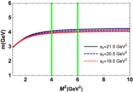
Figure 1: The mass of the hadronic molecule $M_{cc}^{+}$ as a function of the Borel parameter $M^{2}$ at fixed $s_{0}$. Vertical lines show boundaries of working region for $M^{2}$ used in numerical computations.

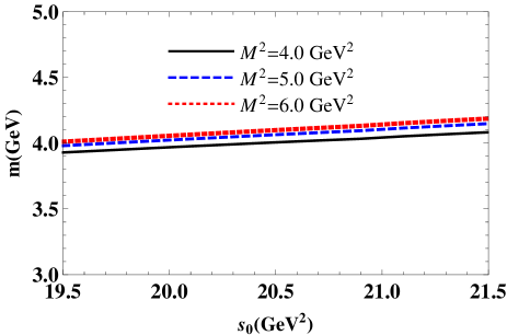
Figure 2: Dependence of $m$ on the continuum threshold parameter $s_{0}$ at fixed $M^{2}$.

The central value of the mass $m$ is above the two-meson $D^{0}D^{\ast}(2010)^{+}$ threshold $3875.1~{}\mathrm{MeV}$, and exceeds the datum of the LHCb collaboration. Even the low estimate for the mass $3930~{}\mathrm{MeV}$ overshoots this boundary. In other words, the dominant decay channel of the molecule $M_{cc}^{+}$ is the process $M_{cc}^{+}\rightarrow D^{0}D^{\ast+}$. In the next section, we are going to calculate the width of $M_{cc}^{+}$ using this decay.

III Width of the decay $M_{cc}^{+}\rightarrow D^{0}D^{\ast+}$

The four-quark state $T_{cc}^{+}$ was observed in $D^{0}D^{0}\pi^{+}$ mass distribution, and therefore it decays strongly to these mesons. The hadronic molecule $M_{cc}^{+}$ has the same quantum numbers and quark content, therefore the process $M_{cc}^{+}\rightarrow D^{0}D^{0}\pi^{+}$ is among possible decay modes of $M_{cc}^{+}$. This decay may proceed through two stages: the process $M_{cc}^{+}\rightarrow D^{0}D^{\ast+}$ followed by the decay $D^{\ast+}\rightarrow D^{0}\pi^{+}$. Our calculations show that the mass of $M_{cc}^{+}$ is enough to generate this chain of transformations.

In this section, we study the decay $M_{cc}^{+}\rightarrow D^{0}D^{\ast+}$ and find the strong coupling $G$ of particles at the vertex $M_{cc}^{+}D^{0}D^{\ast+}$. The QCD three-point sum rule for this coupling can be derived from analysis of the correlation function

$$\Pi_{\mu\nu}(p,p^{\prime})=i^{2}\int d^{4}xd^{4}ye^{i(p^{\prime}y-px)}\langle 0|\mathcal{T}\{J_{\nu}^{D^{\ast}}(y)$$

$$\times J^{D}(0)J_{\mu}^{\dagger}(x)\}|0\rangle,$$ (16)

where $J_{\mu}(x)$, $\ J_{\nu}^{D^{\ast}}(x)$ and $J^{D}(x)$ are the relevant interpolating currents. For the molecule $M_{cc}^{+}$ the current $J_{\mu}(x)$ is given by Eq. (2). The $J_{\nu}^{D^{\ast}}(x)$ and $J^{D}(x)$ are currents of the mesons $D^{\ast+}$ and $D^{0}$, which have the following forms

$$J_{\nu}^{D^{\ast}}(x)=\overline{d}_{i}(x)\gamma_{\nu}c_{i}(x),\ J^{D}(x)=\overline{u}_{j}(x)i\gamma_{5}c_{i}(x),$$ (17)

where $i$ and $j$ are color indices. The 4-momenta of the particles $M_{cc}^{+}$ and $D^{\ast+}$ are $p$ and $p^{\prime}$, respectively, hence the momentum of the $D^{0}$ meson is $q=p-p^{\prime}$.

We continue using standard prescriptions of the sum rule method and, first calculate the correlation function $\Pi_{\mu\nu}(p,p^{\prime})$ in terms of physical parameters of involved particles. Isolating in Eq. (16)  a contribution of the ground-state particles, we get

$$\Pi_{\mu\nu}^{\mathrm{Phys}}(p,p^{\prime})=\frac{\langle 0|J_{\nu}^{D^{\ast}}|D^{\ast+}(p^{\prime},\varepsilon)\rangle\langle 0|J^{D}|D^{0}(q)\rangle}{(p^{2}-m^{2})(p^{\prime 2}-m_{D^{\ast}}^{2})(q^{2}-m_{D}^{2})}$$

$$\times\langle M_{cc}^{+}(p,\epsilon)|J_{\mu}^{\dagger}|0\rangle\langle D^{0}(q)D^{\ast+}(p^{\prime},\varepsilon)|M_{cc}^{+}(p,\epsilon)\rangle+\cdots,$$

(18)

which is the physical side of the sum rule. In Eq. (18) $m_{D^{\ast}}$ and $m_{D}$ are the masses of the $D^{\ast+}$ and $D^{0}$ mesons PDG:2020 , respectively:

$$m_{D^{\ast}} = (2010.26\pm 0.05)~{}\mathrm{MeV},$$

$$m_{D} = (1864.84\pm 0.05)~{}\mathrm{MeV}.$$ (19)

For our purposes, it is necessary to employ the $D^{\ast+}$ and $D^{0}$ mesons’  matrix elements, and, by this way to find compact expression for the function $\Pi_{\mu\nu}^{\mathrm{Phys}}(p,p^{\prime})$. This can be achieved by using the matrix elements

$$\langle 0|J_{\nu}^{D^{\ast}}|D^{\ast+}(p^{\prime},\varepsilon)\rangle=f_{D^{\ast}}m_{D^{\ast}}\varepsilon_{\nu},\$$

$$\langle 0|J^{D}|D^{0}(q)\rangle=\frac{f_{D}m_{D}^{2}}{m_{c}},$$ (20)

where $f_{D^{\ast}}$ and $f_{D}$ are their decay constants, whereas $\varepsilon_{\nu}$ is the polarization vector of the meson $D^{\ast+}$. We model the vertex $\langle D^{0}(q)D^{\ast+}(p^{\prime},\varepsilon)|M_{cc}^{+}(p,\epsilon)\rangle$ by the expression

$$\langle D^{0}(q)D^{\ast+}(p^{\prime},\varepsilon)|M_{cc}^{+}(p,\epsilon)\rangle=G(q^{2})\left[(p\cdot p^{\prime})\right.$$

$$\left.\times(\varepsilon^{\ast}\cdot\epsilon)-(p\cdot\varepsilon^{\ast})(p^{\prime}\cdot\epsilon)\right],$$ (21)

with $G(q^{2})$ being the strong coupling at the vertex $M_{cc}^{+}D^{0}D^{\ast+}$. Then, it is not difficult to show that

$$\Pi_{\mu\nu}^{\mathrm{Phys}}(p,p^{\prime})=G(q^{2})\frac{fmf_{D^{\ast}}m_{D^{\ast}}m_{D}^{2}f_{D}}{m_{c}(p^{2}-m^{2})(p^{\prime 2}-m_{D^{\ast}}^{2})}$$

$$\times\frac{1}{(q^{2}-m_{D}^{2})}\left(\frac{m^{2}+m_{D^{\ast}}^{2}-q^{2}}{2}g_{\mu\nu}-p_{\nu}p_{\mu}^{\prime}\right)+\cdots.$$

(22)

The double Borel transformation of $\Pi_{\mu\nu}^{\mathrm{Phys}}(p,p^{\prime})$ over variables $p^{2}$ and $p^{\prime 2}$ yields

$$\mathcal{B}\Pi_{\mu\nu}^{\mathrm{Phys}}(p,p^{\prime})=G(q^{2})\frac{fmf_{D^{\ast}}m_{D^{\ast}}m_{D}^{2}f_{D}}{m_{c}(q^{2}-m_{D}^{2})}e^{-m^{2}/M_{1}^{2}}$$

$$\times e^{-m_{D^{\ast}}^{2}/M_{2}^{2}}\left(\frac{m^{2}+m_{D^{\ast}}^{2}-q^{2}}{2}g_{\mu\nu}-p_{\nu}p_{\mu}^{\prime}\right)+\cdots.$$

The function $\mathcal{B}\Pi_{\mu\nu}^{\mathrm{Phys}}(p,p^{\prime})$ is the sum of two terms $\sim g_{\mu\nu}$ and $\sim p_{\nu}p_{\mu}^{\prime}$, which may be utilized to obtain the required sum rule. For further studies, we choose the invariant amplitude $\Pi^{\mathrm{Phys}}(p^{2},p^{\prime 2},q^{2})$ corresponding to the structure $\sim g_{\mu\nu}$. The Borel transformation of this amplitude constitutes the physical side of the sum rule.

To determine the QCD side of the three-point sum rule, one should compute $\Pi_{\mu\nu}(p,p^{\prime})$ using quark propagators. As a result, one gets

$$\Pi_{\mu\nu}^{\mathrm{OPE}}(p,p^{\prime})=i^{2}\int d^{4}xd^{4}ye^{i(p^{\prime}y-px)}\left\{\mathrm{Tr}\left[\gamma_{\nu}S_{c}^{ia}(y-x)\right.\right.$$

$$\left.\times\gamma_{\mu}S_{d}^{ai}(x-y)\right]\mathrm{Tr}\left[\gamma_{5}S_{u}^{bj}(x)\gamma_{5}S_{c}^{jb}(-x)\right]$$

$$\left.-\mathrm{Tr}\left[\gamma_{\nu}S_{c}^{ib}(y-x)\gamma_{5}S_{u}^{bj}(x)\gamma_{5}S_{c}^{ja}(-x)\gamma_{\mu}S_{d}^{ai}(x-y)\right]\right\}.$$

(24)

The correlation function $\Pi_{\mu\nu}^{\mathrm{OPE}}(p,p^{\prime})$ is computed by taking into account terms up to dimension $6$, and has structures identical to ones from $\Pi_{\mu\nu}^{\mathrm{Phys}}(p,p^{\prime})$. The explicit expression of $\Pi_{\mu\nu}^{\mathrm{OPE}}(p,p^{\prime})$ is rather lengthy, therefore we do not provide it here.

The double Borel transform of the invariant amplitude $\Pi^{\mathrm{OPE}}(p^{2},p^{\prime 2},q^{2})$ which corresponds to the term $\sim g_{\mu\nu}$ forms the QCD side of the sum rule. By equating the Borel transforms of the amplitudes $\Pi^{\mathrm{OPE}}(p^{2},p^{\prime 2},q^{2})$ and $\Pi^{\mathrm{Phys}}(p^{2},p^{\prime 2},q^{2})$, and carrying out the continuum subtraction, one gets the sum rule for the coupling $G(q^{2})$.

The amplitude $\Pi^{\mathrm{OPE}}(p^{2},p^{\prime 2},q^{2})$ after the Borel transformation and subtraction can be expressed in terms of the spectral density $\rho(s,s^{\prime},q^{2})$ which is determined as a relevant imaginary part of $\Pi_{\mu\nu}^{\mathrm{OPE}}(p,p^{\prime})$,

$$\Pi(\mathbf{M}^{2},\mathbf{s}_{0},q^{2})=\int_{4m_{c}^{2}}^{s_{0}}ds\int_{m_{c}^{2}}^{s_{0}^{\prime}}ds^{\prime}\rho(s,s^{\prime},q^{2})$$

$$\times e^{-s/M_{1}^{2}}e^{-s^{\prime}/M_{2}^{2}}.$$ (25)

Here, $\mathbf{M}^{2}=(M_{1}^{2},M_{2}^{2})$ and $\mathbf{s}_{0}=(s_{0},s_{0}^{\prime})$ are the Borel and continuum threshold parameters, respectively. The sum rule for $G(q^{2})$ is given by the following expression

$$G(q^{2})=\frac{2m_{c}}{fmf_{D^{\ast}}m_{D^{\ast}}m_{D}^{2}f_{D}}\frac{q^{2}-m_{D}^{2}}{m^{2}+m_{D^{\ast}}^{2}-q^{2}}$$

$$\times e^{m^{2}/M_{1}^{2}}e^{m_{D^{\ast}}^{2}/M_{2}^{2}}\Pi(\mathbf{M}^{2},\mathbf{s}_{0},q^{2}).$$ (26)

The coupling $G(q^{2})$ is a function of $q^{2}$ and parameters $(\mathbf{M}^{2},\mathbf{s}_{0})$: the latter, for simplicity, are not written down in Eq. (26) as its arguments. In what follows, we use a new variable $Q^{2}=-q^{2}$ and fix the obtained function by the notation $G(Q^{2})$.

The sum rule Eq. (26) depends on the mass and coupling of the hadronic molecule $M_{cc}^{+}$, which are original results of the current work and have been presented in Eq. (15). The equation (26) also contains the masses and decay constants of the mesons $D^{\ast+}$ and $D^{0}$. The masses of these mesons have been written down in Eq. (19), whereas for their decay constants, we employ

$$f_{D^{\ast}} = (223.5\pm 8.4)~{}\mathrm{MeV},$$

$$f_{D} = (212.6\pm 0.7)~{}\mathrm{MeV}.$$ (27)

Besides these parameters, for computation of $G(Q^{2})$ one should choose working windows for $\mathbf{M}^{2}$ and $\mathbf{s}_{0}$ as well. The restrictions used in such analysis are standard ones for sum rule computations and have been considered above.

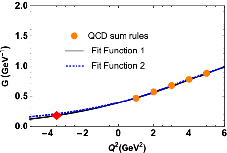
Figure 3: The sum rule results and functions $F(Q^{2})$ (FF 1) and $\overline{F}(Q^{2})$ (FF 2) for the strong coupling $G(Q^{2})$. The red diamond fixes the point $Q^{2}=-m_{D}^{2}$.

The windows for $M_{1}^{2}$ and $s_{0}$ correspond to the $M_{cc}^{+}$ channel and are given by Eq. (14). The parameters $(M_{2}^{2},s_{0}^{\prime})$ for the $D^{\ast+}$ meson’s channel vary inside the intervals

$$M_{2}^{2}\in[2,4]~{}\mathrm{GeV}^{2},\ s_{0}^{\prime}\in[5.5,6.5]~{}\mathrm{GeV}^{2}.$$ (28)

We calculate $G(Q^{2})$ at fixed $Q^{2}=1-6~{}\mathrm{GeV}^{2}$ and plot obtained results in Fig. 3. It is worth noting that at each $Q^{2}$ computations satisfy constraints imposed on parameters $\mathbf{M}^{2}$ and $\mathbf{s}_{0}$ by the sum rule analysis. Thus, in Fig. 4 the coupling $G(Q^{2})$ is depicted as a function of the parameters $M_{1}^{2}$ and $M_{2}^{2}$ at $Q^{2}=1~{}\mathrm{GeV}^{2}$ and middle of the regions $s_{0}$ and $s_{0}^{\prime}$. A relative stability of $G(1\ \mathrm{GeV}^{2})$ upon changing of $\mathbf{M}^{2}$ is evident: Variations of $M_{1}^{2}$ and $M_{2}^{2}$ within explored regions do not exceed $30\%$ of the central value for $G(1\ \mathrm{GeV}^{2})$. Numerically, we find

$$G(1\ \mathrm{GeV}^{2})=0.48_{-0.09}^{+0.14}~{}\mathrm{GeV}^{-1}.$$ (29)

Figure 4: The strong coupling $G=G(1~{}\mathrm{GeV}^{2})$ as a function of the Borel parameters $M_{1}^{2}$ and $M_{2}^{2}$ at $s_{0}=20.5~{}\mathrm{GeV}^{2}$ and $s_{0}^{\prime}=6~{}\mathrm{GeV}^{2}$.

The width of the process $M_{cc}^{+}\rightarrow D^{0}D^{\ast+}$ is determined by the coupling $G$ at the mass shell $q^{2}=m_{D}^{2}$ of the meson $D^{0}$, which cannot be calculated directly using the sum rule method. To avoid this difficulty, we introduce fit functions $F(Q^{2})$ and $\overline{F}(Q^{2})$ that for the momenta $Q^{2}>0$ give results identical to QCD sum rule’s ones, but can be extrapolated to the region of $Q^{2}<0$ to fix $G$. We employ the fit functions $F(Q^{2})$ and $\overline{F}(Q^{2})$ given by the expressions

$$F(Q^{2})=F_{0}\mathrm{\exp}\left[c_{1}\frac{Q^{2}}{m^{2}}+c_{2}\left(\frac{Q^{2}}{m^{2}}\right)^{2}\right],$$ (30)

and

$$\overline{F}(Q^{2})=\frac{\overline{F}_{0}}{\left(1-\frac{Q^{2}}{m^{2}}\right)\left(1-\sigma_{1}\frac{Q^{2}}{m^{2}}+\sigma_{2}\left(\frac{Q^{2}}{m^{2}}\right)^{2}\right)},$$ (31)

where $F_{0}$, $c_{1}$ and $c_{2}$ and $\overline{F}_{0}$, $\sigma_{1}$ and $\sigma_{2}$ are fitting parameters. From numerical computations, it is not difficult to find that $F_{0}=0.39~{}\mathrm{GeV}^{-1},$ $c_{1}=3.29$ and $c_{2}=-1.95$. Similar analysis gives $\overline{F}_{0}=0.39~{}\mathrm{GeV}^{-1},$ $\sigma_{1}=2.11$ and $\sigma_{2}=2.97$. In Fig. 3, along with the sum rule results for $G(Q^{2})$, we plot also the functions $F(Q^{2})$ and $\overline{F}(Q^{2})$. It is seen, that there are nice agreements between the fit functions and QCD data. Their predictions for the coupling $G$ are also very close to each other, and generate only small additional uncertainties $\pm 0.01$ in $G$.

The functions $F(Q^{2})$ and $\overline{F}(Q^{2})$ at the $D^{0}$ meson’s mass shell lead to the average result

$$G=(0.192\pm 0.061)~{}\mathrm{GeV}^{-1},$$ (32)

where the theoretical errors are the sum (in quadrature) of uncertainties coming from sum rule computations $\pm 0.06$ and ones due to fitting procedures. The width of decay $M_{cc}^{+}\rightarrow D^{0}D^{\ast+}$ is determined by the expression

$$\Gamma\left[M_{cc}^{+}\rightarrow D^{0}D^{\ast+}\right]=G^{2}\frac{m_{D^{\ast}}^{2}\lambda\left(m,m_{D^{\ast}},m_{D}\right)}{24\pi}$$

$$\times\left(3+\frac{2\lambda^{2}\left(m,m_{D^{\ast}},m_{D}\right)}{m_{D^{\ast}}^{2}}\right),$$ (33)

where

$$\lambda\left(a,b,c\right)=\frac{1}{2a}\sqrt{a^{4}+b^{4}+c^{4}-2\left(a^{2}b^{2}+a^{2}c^{2}+b^{2}c^{2}\right)}.$$ (34)

Using the strong coupling from Eq. (32), one can evaluate width of the process $M_{cc}^{+}\rightarrow D^{0}D^{\ast+}$

$$\Gamma\left[M_{cc}^{+}\rightarrow D^{0}D^{\ast+}\right]=(3.8\pm 1.7)~{}\mathrm{MeV}.$$ (35)

There are also other decay modes of the molecule $M_{cc}^{+}$, which produce mesons $D^{0}D^{0}\pi^{+}$ or $D^{0}D^{+}\pi^{0}$. They run through creation of intermediate scalar tetraquarks followed by their decays to a pair of conventional mesons Agaev:2021vur . These modes establish the main mechanism for strong decays of $T_{cc}^{+}$, but are subdominant processes for the molecule $M_{cc}^{+}$, and therefore can be neglected. Our prediction for the width of $M_{cc}^{+}$ demonstrates that it is a relatively wide resonance.

IV Discussion and conclusions

We have calculated the mass and width of the doubly charmed axial-vector state with quark content $cc\overline{u}\overline{d}$ by modeling it as the hadronic molecule $M_{cc}^{+}=D^{0}D^{\ast+}$. Predictions obtained for the mass $m=(4060\pm 130)~{}\mathrm{MeV}$ and width $\Gamma=(3.8\pm 1.7)~{}\mathrm{MeV}$ of this molecule exceed the LHCb data Aaij:2021vvq ; LHCb:2021auc . In our previous work, we carried out similar analysis by treating the axial-vector $T_{cc}^{+}=cc\overline{u}\overline{d}$ state in the context of the tetraquark model Agaev:2021vur . Parameters of the exotic meson $T_{cc}^{+}$ agree nicely with data of the LHCb collaboration. Comparing with each another results extracted from the sum rules in tetraquark and molecule models, we see that the molecule $M_{cc}^{+}$ is heavier and wider than the tetraquark structure.

Actually one might expect such outcome, because colored diquark and antidiquark compact to form tightly-bound state, whereas interaction of two colorless mesons is less intensive. Decays of tetraquarks and molecules to conventional mesons also differ from each other. Indeed, in the case of a tetraquark these processes require reorganization of its quark structure. Contrary, a hadronic molecule’s dissociation is free of such obstacles. Hence, hadronic molecules are usually heavier and wider than their tetraquark counterparts.

In this regards, it is instructive to recall a situation with the resonance $X_{0}(2900)$ discovered also by the LHCb collaboration. In Ref. Agaev:2020nrc , we investigated $X_{0}$ and evaluated its parameters. Results obtained for the mass and width of $X_{0}$ allowed us to interpret it as the hadronic molecule $\overline{D}^{\ast}K^{\ast}$. We argued additionally that a ground-state $1S$ scalar tetraquark with the same content should have considerably smaller mass. This conclusion was supported by analysis of Ref. He:2020jna , in which $X_{0}$ was considered as the radially excited $2S$ tetraquark $[ud][\overline{s}\overline{c}]$. The mass difference between $1S$ and $2S$ particles equals there to $\approx 500~{}\mathrm{MeV}$. Because the molecule $\overline{D}^{\ast}K^{\ast}$ and $2S$ tetraquark $[ud][\overline{s}\overline{c}]$ have approximately equal masses, the same estimate is valid for a mass gap between the molecule $\overline{D}^{\ast}K^{\ast}$ and ground state tetraquark. In the case of the exotic mesons $M_{cc}^{+}$ and $T_{cc}^{+}$ this mass difference amounts to approximately $200$ $\mathrm{MeV}$ being in a qualitative agreement with the above analysis.

The molecule $M_{cc}^{+}$ was considered using the QCD sum rule method also in other articles. Thus, in Ref. Dias:2011mi the mass of $M_{cc}^{+}$ was estimated indirectly using the spectral sum rule prediction for the ratio between the masses of $M_{cc}^{+}$ and resonance $X(3872)$. Let us note that relevant calculations were carried by taking into account condensates up to dimension-$6$. The prediction $m=(3872.2\pm 39.5)~{}\mathrm{MeV}$ obtained there for the mass of $M_{cc}^{+}$ is below two-meson threshold and close to the LHCb data.

Direct sum rule computations of parameters of doubly charmed axial-vector states $cc\overline{u}\overline{d}$ were performed in Refs. Xin:2021wcr ; Wang:2017dtg . In the tetraquark model the mass of such state was predicted within the range Wang:2017dtg

$$\widetilde{m}=(3900\pm 90)~{}\mathrm{MeV}.$$ (36)

This is higher than the LHCb data, and exceeds also our result $(3868\pm 124)~{}\mathrm{MeV}$ for this model from Ref. Agaev:2021vur .

The axial-vector isoscalar and isovector molecules built of mesons $D^{0}$ and $D^{\ast+}$ were explored in Ref. Xin:2021wcr , in which their masses were found equal to

$$m_{\mathrm{I=0}} = (3880\pm 110)~{}\mathrm{MeV},$$

$$m_{\mathrm{I=1}} = (3890\pm 110)~{}\mathrm{MeV},$$ (37)

respectively. The isoscalar molecule was interpreted as the LHCb resonance $T_{cc}^{+}$, or its essential component. Of course, comparing Eqs. (15) and (37) one sees overlapping regions for the mass of $M_{cc}^{+}$, but there are essential differences between relevant central values.

It is interesting that masses of the tetraquark and molecule states from Eqs. (36) and (37) coincide with each other. This fact may be explained by different choices for the renormalization/factorization scale $\mu$ used to evolve vacuum condensates and quark masses. Indeed, $\widetilde{m}$ was obtained at $\mu=1.3~{}\mathrm{GeV}$, whereas $m_{\mathrm{I}}$ extracted by employing the scale $\mu=1.4~{}\mathrm{GeV}$. Different scales presumably eliminate a typical mass gap between tetraquark and molecule structures. The choice for the scale $\mu>1\ \mathrm{GeV}$ may also generate the discrepancy between Eq. (37) and our result for the molecule $D^{0}D^{\ast+}$. It is worth to note that Eq. (15) have been obtained at $\mu=1~{}\mathrm{GeV}$, which is necessary for leading-order QCD calculations.

To fix the scale $\mu$ unambiguously and damp sensitivity of results against its variations, one needs to find physical quantities with the next-to-leading order (NLO) accuracy: The NLO results have enhanced predictive power, and their comparisons with data lead to more reliable conclusions. The factorized NLO perturbative corrections to doubly heavy exotic mesons’ masses and couplings were computed in Ref. Albuquerque:2022weq in QCD Inverse Laplace sum rule approach. These corrections are important to legitimate the choice of heavy quark masses used in relevant studies, though in the $\overline{\mathrm{MS}}$ scheme NLO effects themselves are small Albuquerque:2022weq . The authors explained by this fact success of corresponding leading-order QCD analyses. It is possible to carry out similar NLO computations in the context of the two-point sum rule method to remove ambiguities in the choice of the scale $\mu$ while calculating parameters of $T_{cc}^{+}$ and $M_{cc}^{+}$, which, however, are beyond the scope of the current article.

Summing up, investigations of $T_{cc}^{+}$ and $M_{cc}^{+}$ in the framework of QCD sum rule method lead for these states to wide diversity of predictions. The sum rule method relies on fundamental principles of QCD and uses universal vacuum condensates to extract parameters of various hadrons, nevertheless it suffers from theoretical errors which make difficult unambiguous interpretation of obtained results. Thus, predictions for the mass and width of the hadronic molecule $M_{cc}^{+}$ obtained in the current article differ from relevant LHCb data, but these differences remain within $1.5$ and $2$ standard deviations, respectively. Therefore, though our studies demonstrate that a preferable assignment for the LHCb resonance is the tetraquark model $T_{cc}^{+}$, within the theoretical uncertainties, they also do not rule out the molecule picture $M_{cc}^{+}\equiv D^{0}D^{\ast+}$.

Controversial predictions for parameters of the molecule $M_{cc}^{+}$ were made in the context of alternative methods Meng:2021jnw ; Ling:2021bir ; Chen:2021vhg as well. Results for the full width of the $M_{cc}^{+}$ obtained in papers Meng:2021jnw ; Ling:2021bir are rather small compared with the LHCb data. At the same time, a nice agreement with recent measurements was declared in Ref. Chen:2021vhg . Moreover, in this work the authors predicted existence of another doubly charmed resonance with the mass $m=3876~{}\mathrm{MeV}$ and width $\Gamma=412~{}\mathrm{keV}$.

As is seen, even in the context of same models and methods, theoretical investigations sometimes lead to contradictory predictions for the parameters of the molecule $M_{cc}^{+}$: New efforts are required to settle existing problems. Additionally, more accurate LHCb data are necessary for the full width of the doubly charmed state $T_{cc}^{+}$ to compare with different theoretical results.

*

Appendix A The propagators $S_{q(Q)}(x)$ and invariant amplitude $\Pi(M^{2},s_{0})$

In the current article, for the light quark propagator $S_{q}^{ab}(x)$, we employ the following expression

$$S_{q}^{ab}(x)=i\delta_{ab}\frac{\not{x}}{2\pi^{2}x^{4}}-\delta_{ab}\frac{m_{q}}{4\pi^{2}x^{2}}-\delta_{ab}\frac{\langle\overline{q}q\rangle}{12}+i\delta_{ab}\frac{\not{x}m_{q}\langle\overline{q}q\rangle}{48}-\delta_{ab}\frac{x^{2}}{192}\langle\overline{q}g_{s}\sigma Gq\rangle$$

$$+i\delta_{ab}\frac{x^{2}\not{x}m_{q}}{1152}\langle\overline{q}g_{s}\sigma Gq\rangle-i\frac{g_{s}G_{ab}^{\alpha\beta}}{32\pi^{2}x^{2}}\left[\not{x}{\sigma_{\alpha\beta}+\sigma_{\alpha\beta}}\not{x}\right]-i\delta_{ab}\frac{x^{2}\not{x}g_{s}^{2}\langle\overline{q}q\rangle^{2}}{7776}$$

$$-\delta_{ab}\frac{x^{4}\langle\overline{q}q\rangle\langle g_{s}^{2}G^{2}\rangle}{27648}+\cdots.$$ (A.38)

For the heavy quark $Q=c$, we use the propagator $S_{Q}^{ab}(x)$

$$S_{Q}^{ab}(x)=i\int\frac{d^{4}k}{(2\pi)^{4}}e^{-ikx}\Bigg{\{}\frac{\delta_{ab}\left({\not{k}}+m_{Q}\right)}{k^{2}-m_{Q}^{2}}-\frac{g_{s}G_{ab}^{\alpha\beta}}{4}\frac{\sigma_{\alpha\beta}\left({\not{k}}+m_{Q}\right)+\left({\not{k}}+m_{Q}\right)\sigma_{\alpha\beta}}{(k^{2}-m_{Q}^{2})^{2}}$$

$$+\frac{g_{s}^{2}G^{2}}{12}\delta_{ab}m_{Q}\frac{k^{2}+m_{Q}{\not{k}}}{(k^{2}-m_{Q}^{2})^{4}}+\frac{g_{s}^{3}G^{3}}{48}\delta_{ab}\frac{\left({\not{k}}+m_{Q}\right)}{(k^{2}-m_{Q}^{2})^{6}}\left[{\not{k}}\left(k^{2}-3m_{Q}^{2}\right)+2m_{Q}\left(2k^{2}-m_{Q}^{2}\right)\right]\left({\not{k}}+m_{Q}\right)+\cdots\Bigg{\}}.$$

Here, we have used the short-hand notations

$$G_{ab}^{\alpha\beta}\equiv G_{A}^{\alpha\beta}\lambda_{ab}^{A}/2,\ \ G^{2}=G_{\alpha\beta}^{A}G_{A}^{\alpha\beta},\ G^{3}=f^{ABC}G_{\alpha\beta}^{A}G^{B\beta\delta}G_{\delta}^{C\alpha},$$ (A.40)

where $G_{A}^{\alpha\beta}$ is the gluon field strength tensor, $\lambda^{A}$ and $f^{ABC}$ are the Gell-Mann matrices and structure constants of the color group $SU_{c}(3)$, respectively. The indices $A,B,C$ run in the range $1,2,\ldots 8$.

The invariant amplitude $\Pi(M^{2},s_{0})$ obtained after the Borel transformation and subtraction procedures is given by Eq. (10)

$$\Pi(M^{2},s_{0})=\int_{4m_{c}^{2}}^{s_{0}}ds\rho^{\mathrm{OPE}}(s)e^{-s/M^{2}}+\Pi(M^{2}),$$

where the spectral density $\rho^{\mathrm{OPE}}(s)$ and the function $\Pi(M^{2})$ are determined by formulas

$$\rho^{\mathrm{OPE}}(s)=\rho^{\mathrm{pert.}}(s)+\sum_{N=3}^{8}\rho^{\mathrm{DimN}}(s),\ \ \Pi(M^{2})=\sum_{N=6}^{10}\Pi^{\mathrm{DimN}}(M^{2}),$$ (A.41)

respectively. The components of $\rho^{\mathrm{OPE}}(s)$ and $\Pi(M^{2})$ are given by the expressions

$$\rho^{\mathrm{DimN}}(s)=\int_{0}^{1}d\alpha\int_{0}^{1-a}d\beta\rho^{\mathrm{DimN}}(s,\alpha,\beta),\ \ \rho^{\mathrm{DimN}}(s)=\int_{0}^{1}d\alpha\rho^{\mathrm{DimN}}(s,\alpha),$$ (A.42)

and

$$\Pi^{\mathrm{DimN}}(M^{2})=\int_{0}^{1}d\alpha\int_{0}^{1-a}d\beta\Pi^{\mathrm{DimN}}(M^{2},\alpha,\beta),\ \ \Pi^{\mathrm{DimN}}(M^{2})=\int_{0}^{1}d\alpha\Pi^{\mathrm{DimN}}(M^{2},\alpha).$$ (A.43)

depending on whether $\rho$ and $\Pi(M^{2})$ are functions of $\alpha$ and $\beta$ or only of $\alpha$. In Eqs. (A.42) and (A.43) variables $\alpha$ and $\beta$ are Feynman parameters.

The perturbative and nonperturbative components of the spectral density $\rho^{\mathrm{pert.}}(s,\alpha,\beta)$ and $\rho^{\mathrm{Dim3(4,5,6,7,8)}}(s,\alpha,\beta)$  have the forms:

$$\rho^{\mathrm{pert.}}(s,\alpha,\beta)=\frac{\Theta(L_{1})}{49152\pi^{6}L^{2}N_{1}^{8}}\left[m_{c}^{2}N_{2}-s\alpha\beta L\right]^{2}\left\{s^{2}\alpha^{2}\beta^{2}L^{3}\left[18\beta^{2}+18\alpha(\alpha-1)-\beta(18+325\alpha)\right]+m_{c}^{4}N_{1}^{2}\left[18\beta^{5}\right.\right.$$

$$\left.+18\alpha^{3}(\alpha-1)^{2}+\beta^{4}(37\alpha-36)+\beta^{2}\alpha(54-110\alpha+29\alpha^{2})+\beta^{3}(18-91\alpha+29\alpha^{2})+\beta\alpha^{2}(54-91\alpha+37\alpha^{2})\right]$$

$$-2m_{c}^{2}s\alpha\beta\left[18\beta^{7}+18\alpha^{3}(\alpha-1)^{4}-3\beta\alpha^{2}(\alpha-1)^{3}(18+13\alpha)-3\beta^{6}(24+13\alpha)+\beta^{5}(108+63\alpha-296\alpha^{2})\right.$$

$$-2\beta^{2}\alpha(\alpha-1)^{2}(-27-3\alpha+148\alpha^{2})+\beta^{4}(-72+45\alpha+598\alpha^{2}-571\alpha^{3})+\beta^{3}\left(18-123\alpha-254\alpha^{2}+930\alpha^{3}\right.$$

$$\left.\left.\left.-517\alpha^{4}\right)\right]\right\},$$ (A.44)

$$\rho^{\mathrm{Dim3}}(s,\alpha,\beta)=\frac{m_{c}\Theta(L_{1})}{512\pi^{4}N_{1}^{5}}\left[m_{c}^{2}N_{2}-s\alpha\beta L\right]\left\{2\langle\overline{d}d\rangle(11\beta-\alpha)\left[m_{c}^{2}N_{2}-2s\alpha\beta L\right]-\langle\overline{u}u\rangle(\beta-11\alpha)\left[m_{c}^{2}N_{2}-3s\alpha\beta L\right]\right\},$$ (A.45)

$$\rho^{\mathrm{Dim4}}(s,\alpha,\beta)=\frac{\langle\alpha_{s}G^{2}/\pi\rangle\Theta(L_{1})}{73728\pi^{4}(\beta-1)L^{2}N_{1}^{6}}\left\{-s^{2}(\beta-1)\alpha^{2}\beta^{2}L^{2}\left[18\beta^{4}+6\alpha(\alpha-1)^{2}(3\alpha-2)+3\beta^{3}(417\alpha-16)\right.\right.$$

$$\left.+\beta^{2}(42-1521\alpha-91\alpha^{2})-3\beta(4-94\alpha-333\alpha^{2}+423\alpha^{3})\right]-m_{c}^{4}N_{1}^{2}\left[18\beta^{8}+\beta^{7}(611\alpha-108)\right.$$

$$+\beta^{6}(228-2053\alpha+1918\alpha^{2})-6\alpha^{3}(\alpha-1)^{2}(2-9\alpha+3\alpha^{2}+2\alpha^{3})+\beta^{5}(-216+2567\alpha-5375\alpha^{2}+2181\alpha^{3})$$

$$+\beta^{4}(90-1455\alpha+5518\alpha^{2}-5083\alpha^{3}+857\alpha^{4})+\beta\alpha^{2}(-36+342\alpha-555\alpha^{2}+248\alpha^{3}+23\alpha^{4}-22\alpha^{5})$$

$$-\beta^{3}(12-366\alpha+2565\alpha^{2}-4315\alpha^{3}+1686\alpha^{4}+94\alpha^{5})-\beta^{2}\alpha\left(36-540\alpha+1743\alpha^{2}-1306\alpha^{3}+16\alpha^{4}\right.$$

$$\left.+105\alpha^{5}\right)+2m_{c}^{2}s\alpha\beta\left[15\beta^{10}+13\beta^{9}(74\alpha-9)+\beta^{8}(372-5060\alpha+3754\alpha^{2})-3\alpha^{3}(\alpha-1)^{4}(4-14\alpha+5\alpha^{2}+2\alpha^{3})\right.$$

$$+\beta^{7}\left(-630+10956\alpha-17152\alpha^{2}+6047\alpha^{3}\right)-\beta\alpha^{2}(\alpha-1)^{3}(-36+348\alpha+174\alpha^{2}-439\alpha^{3}+11\alpha^{4})$$

$$+\beta^{6}\left(615-12500\alpha+31809\alpha^{2}-23517\alpha^{3}+4514\alpha^{4}\right)+\beta^{5}\left(-345+7970\alpha-30691\alpha^{2}+36238\alpha^{3}-13408\alpha^{4}+160\alpha^{5}\right)$$

$$-\beta^{2}\alpha(\alpha-1)^{2}\left(36-672\alpha+1809\alpha^{2}+1220\alpha^{3}-2788\alpha^{4}+538\alpha^{5}\right)+\beta^{4}\left(102-2772\alpha+16465\alpha^{2}-28426\alpha^{3}+14658\alpha^{4}\right.$$

$$\left.\left.\left.+2648\alpha^{5}-2675\alpha^{6}\right)-\beta^{3}\left(12-480\alpha+4893\alpha^{2}-12403\alpha^{3}+7946\alpha^{4}+6091\alpha^{5}-8153\alpha^{6}+2094\alpha^{7}\right)\right]\right\},$$ (A.46)

$$\rho^{\mathrm{Dim5}}(s,\alpha,\beta) = -\frac{m_{c}\Theta(L_{1})L}{1024\pi^{4}N_{1}^{4}}\left\{-\langle\overline{u}g_{s}\sigma Gu\rangle(\beta-11\alpha)\left[m_{c}^{2}N_{2}-2s\alpha\beta L\right]\right.$$ (A.47)

$$\left.+\langle\overline{d}g_{s}\sigma Gd\rangle(11\beta-\alpha)\left[m_{c}^{2}N_{2}-3s\alpha\beta L\right]\right\},$$

$$\rho_{1}^{\mathrm{Dim6}}(M^{2},\alpha,\beta)=\frac{\langle g_{s}^{3}G^{3}\rangle\Theta(L_{1})}{45\cdot 2^{19}\pi^{6}L^{2}N_{1}^{7}}\left\{36m_{c}^{2}N_{1}^{2}\left[12\beta^{9}-5\beta^{4}\alpha^{5}-4\beta^{3}\alpha^{5}(\alpha-1)+12\beta\alpha^{5}(\alpha-1)^{3}+12\alpha^{6}(\alpha-1)^{3}\right.\right.$$

$$+4\beta^{8}(8\alpha-9)+\beta^{2}\alpha^{5}(13-18\alpha+5\alpha^{2})+\beta^{7}(36-76\alpha+45\alpha^{2})+3\beta^{5}\alpha(-4+11\alpha-12\alpha^{2}+5\alpha^{3})+2\beta^{6}\left(-6\right.$$

$$\left.\left.+28\alpha-39\alpha^{2}+18\alpha^{3}\right)\right]-s\alpha\beta L^{2}\left[216\beta^{9}+216\alpha^{6}(\alpha-1)^{3}-24\beta\alpha^{5}(\alpha-1)^{2}(3+73\alpha)-24\beta^{8}(27+73\alpha)\right.$$

$$+\beta^{2}\alpha^{4}(\alpha-1)^{2}(144+2773\alpha)+\beta^{3}\alpha^{4}(-543-1759\alpha+2302\alpha^{2})+\beta^{7}(648+3432\alpha+2611\alpha^{2})$$

$$-3\beta^{4}\alpha^{2}(-48+235\alpha-544\alpha^{2}+357\alpha^{3})+2\beta^{6}(-108-804\alpha-2539\alpha^{2}+989\alpha^{3})$$

$$\left.-\beta^{5}\alpha(72-2323\alpha+1273\alpha^{2}+1233\alpha^{3})\right]+72m_{c}^{2}\left[2\beta^{13}+2\alpha^{8}(\alpha-1)^{5}-\beta\alpha^{7}(\alpha-1)^{4}(6+\alpha)-\beta^{12}(10+\alpha)\right.$$

$$+\beta^{11}(20-2\alpha-5\alpha^{2})-\beta^{2}\alpha^{6}(\alpha-1)^{3}(-6+10\alpha+5\alpha^{2})+\beta^{3}\alpha^{5}(\alpha-1)^{3}(2-21\alpha+8\alpha^{2})+\beta^{4}\alpha^{5}(\alpha-1)^{2}$$

$$\times(12-46\alpha+31\alpha^{2})+\beta^{10}(-20+18\alpha+5\alpha^{2}+8\alpha^{3})+\beta^{5}\alpha^{3}(\alpha-1)^{2}(-2+8\alpha-30\alpha^{2}+41\alpha^{3})+\beta^{9}\left(10-32\alpha\right.$$

$$\left.+21\alpha^{2}-45\alpha^{3}+31\alpha^{4}\right)+\beta^{8}(-2+23\alpha-43\alpha^{2}+89\alpha^{3}-108\alpha^{4}+41\alpha^{5})+\beta^{7}\alpha\left(-6+28\alpha-77\alpha^{2}+135\alpha^{3}\right.$$

$$\left.\left.\left.-112\alpha^{4}+32\alpha^{5}\right)+\beta^{6}\alpha^{2}(-6+27\alpha-70\alpha^{2}+109\alpha^{3}-92\alpha^{4}+32\alpha^{5})\right]\right\},$$ (A.48)

$$\rho_{1}^{\mathrm{Dim7}}(M^{2},\alpha,\beta)=\frac{m_{c}\langle\alpha_{s}G^{2}/\pi\rangle\Theta(L_{1})}{4608\pi^{2}N_{1}^{4}}\left\{2\langle\overline{d}d\rangle\left[25\beta^{5}-2\beta^{4}(14+19\alpha)+\beta^{3}(3+65\alpha-68\alpha^{2})\right.\right.$$

$$\left.+\beta^{2}\alpha(-27+84\alpha-56\alpha^{2})+\beta\alpha^{2}(-27+53\alpha-26\alpha^{2})+\alpha^{3}(3-4\alpha+\alpha^{2})\right]$$

$$+\langle\overline{u}u\rangle\left[-5\beta^{5}+\beta^{4}(8+22\alpha)+\beta\alpha^{2}(27-37\alpha+10\alpha^{2})+\alpha^{3}(-3-16\alpha+19\alpha^{2})\right.$$

$$\left.\left.+\beta^{2}\alpha(27-72\alpha+34\alpha^{2})+\beta^{3}(-3-49\alpha+46\alpha^{2})\right]\right\},$$ (A.49)

$$\rho_{1}^{\mathrm{Dim8}}(M^{2},\alpha,\beta)=-\frac{\langle\alpha_{s}G^{2}/\pi\rangle^{2}}{24576\pi^{2}N_{1}^{3}}\Theta(L_{1})\alpha\beta L.$$ (A.50)

The components $\rho^{\mathrm{Dim6(7,8)}}(s,\alpha)$ are given by the formulas

$$\rho_{2}^{\mathrm{Dim6}}(s,\alpha)=\frac{\langle\overline{d}d\rangle\langle\overline{u}u\rangle}{192\pi^{2}}\Theta(L_{2})\left[13m_{c}^{2}+3s\alpha(\alpha-1)\right],\ \$$ (A.51)

$$\rho_{2}^{\mathrm{Dim7}}(s,\alpha)=\frac{m_{c}\langle\alpha_{s}G^{2}/\pi\rangle}{9216\pi^{2}}\Theta(L_{2})\left[\langle\overline{u}u\rangle(1-12\alpha)+\langle\overline{d}d\rangle(-22+24\alpha)\right],\$$ (A.52)

and

$$\rho_{2}^{\mathrm{Dim8}}(s,\alpha)=\frac{\langle\overline{d}d\rangle\langle\overline{u}g_{s}\sigma Gu\rangle}{48\pi^{2}}\Theta(L_{2})\alpha(\alpha-1).\$$ (A.53)

Components of the function $\Pi(M^{2})$ are:

$$\Pi^{\mathrm{Dim6}}(M^{2},\alpha,\beta)=\frac{m_{c}^{4}\langle g_{s}^{3}G^{3}\rangle}{45\cdot 2^{18}\pi^{6}\alpha\beta(\beta-1)L^{3}N_{1}^{4}}\exp\left[-\frac{m_{c}^{2}N_{2}}{M^{2}\alpha\beta L}\right]\left[29\beta^{11}-(\alpha-1)^{3}\alpha^{7}(99+70\alpha)\right.$$

$$+\beta^{10}(-186+113\alpha)+\beta^{9}(384-447\alpha-50\alpha^{2})-\beta(\alpha-1)^{2}\alpha^{6}(-108+212\alpha+111\alpha^{2})$$

$$+\beta^{8}(-326+663\alpha+200\alpha^{2}-447\alpha^{3})+\beta^{6}\alpha(108+340\alpha-1886\alpha^{2}+2485\alpha^{3}-1042\alpha^{4})$$

$$+\beta^{7}(99-437\alpha-370\alpha^{2}+1510\alpha^{3}-880\alpha^{4})+\beta^{5}\alpha^{2}(-120+1030\alpha-2607\alpha^{2}+2577\alpha^{3}-740\alpha^{4})$$

$$+\beta^{4}\alpha^{3}(-207+1209\alpha-2358\alpha^{2}+1593\alpha^{3}-377\alpha^{4})+\beta^{3}\alpha^{4}\left(-270+943\alpha-1143\alpha^{2}\right.$$

$$\left.\left.+527\alpha^{3}-120\alpha^{4}\right)+\beta^{2}\alpha^{5}(-120+112\alpha+179\alpha^{2}-74\alpha^{3}-97\alpha^{4})\right],$$ (A.54)

$$\Pi^{\mathrm{Dim7}}(M^{2},\alpha,\beta)=\frac{m_{c}\langle\alpha_{s}G^{2}/\pi\rangle}{4608\pi^{2}M^{2}\alpha\beta L^{2}N_{1}^{4}}\left\{M^{2}\alpha^{2}\beta^{2}L^{3}[2\langle\overline{d}d\rangle(11\beta^{2}-\alpha^{2})+\langle\overline{u}u\rangle(11\alpha^{2}-\beta^{2})]\right.$$

$$+m_{c}^{4}\langle\overline{u}u\rangle N_{1}^{2}\exp\left[-\frac{m_{c}^{2}N_{2}}{M^{2}\alpha\beta L}\right]\left[10\beta^{5}+10\alpha^{4}(\alpha-1)+\beta^{4}(-10+19\alpha)+\beta^{3}\alpha(-20+29\alpha)\right.$$

$$\left.+\beta\alpha^{3}(-20+31\alpha)+\beta^{2}\alpha^{2}(-20+41\alpha)\right]+m_{c}^{2}\langle\overline{d}d\rangle\exp\left[-\frac{m_{c}^{2}N_{2}}{M^{2}\alpha\beta L}\right]\left[m_{c}^{2}N_{1}^{2}\left(10\beta^{5}+10\alpha^{4}(\alpha-1)\right.\right.$$

$$\left.+\beta\alpha^{3}(-20+19\alpha)+\beta^{2}\alpha^{2}(-20+29\alpha)+\beta^{4}(-10+31\alpha)+\beta^{3}\alpha(-20+41\alpha)\right)$$

$$-M^{2}\alpha\beta\left(10\beta^{7}+10\alpha^{4}(\alpha-1)^{3}+\alpha^{3}\beta(\alpha-1)^{2}(-20+29\alpha)+\beta^{6}(-30+41\alpha)+2\beta^{5}(15-51\alpha+41\alpha^{2})\right.$$

$$+\beta^{2}\alpha^{2}(-20+99\alpha-137\alpha^{2}+58\alpha^{3})+\beta^{3}\alpha(-20+111\alpha-180\alpha^{2}+89\alpha^{3})$$

$$\left.\left.\left.+\beta^{4}(-10+81\alpha-173\alpha^{2}+101\alpha^{3})\right)\right]\right\},$$ (A.55)

$$\Pi^{\mathrm{Dim8}}(M^{2},\alpha,\beta)=\frac{\langle\alpha_{s}G^{2}/\pi\rangle^{2}}{27\cdot 2^{13}\pi^{2}M^{4}\alpha^{2}\beta^{2}L^{4}N_{1}^{3}}\left\{3M^{4}\alpha^{3}\beta^{3}L^{5}+m_{c}^{2}\exp\left[-\frac{m_{c}^{2}N_{2}}{M^{2}\alpha\beta L}\right]\left\{8m_{c}^{4}\alpha^{2}\beta^{2}N_{1}^{2}\right.\right.$$

$$\times\left[2\beta^{3}+2\alpha^{2}(\alpha-1)+\alpha\beta(-4+5\alpha)+\beta^{2}(-2+5\alpha)\right]-8m_{c}^{2}M^{2}\left[3\beta^{11}+3\alpha^{6}(\alpha-1)^{5}+3\beta^{10}(-5+7\alpha)\right.$$

$$+3\beta\alpha^{5}(\alpha-1)^{4}(-4+7\alpha)+\beta^{9}(30-96\alpha+74\alpha^{2})+\beta^{2}\alpha^{4}(\alpha-1)^{3}(21-84\alpha+74\alpha^{2})$$

$$+3\beta^{8}(-10+58\alpha-102\alpha^{2}+57\alpha^{3})+\beta^{3}\alpha^{3}(\alpha-1)^{2}(-24+153\alpha-295\alpha^{2}+171\alpha^{3})$$

$$+\beta^{4}\alpha^{2}(\alpha-1)^{2}(-21+159\alpha-385\alpha^{2}+286\alpha^{3})+\beta^{7}(15-156\alpha+495\alpha^{2}-637\alpha^{3}+286\alpha^{4})$$

$$+\beta^{5}\alpha(-12+147\alpha-625\alpha^{2}+1215\alpha^{3}-1091\alpha^{4}+366\alpha^{5})+\beta^{6}\left(-3+69\alpha-389\alpha^{2}+914\alpha^{3}\right.$$

$$\left.\left.-957\alpha^{4}+366\alpha^{5}\right)\right]+M^{4}\alpha\beta\left[48\beta^{9}+48\alpha^{4}(\alpha-1)^{5}+3\beta^{8}(-80+71\alpha)+3\beta\alpha^{3}(\alpha-1)^{4}(-23+71\alpha)\right.$$

$$+2\beta^{2}\alpha^{2}(\alpha-1)^{3}(21-180\alpha+239\alpha^{2})+\beta^{7}(480-921\alpha+478\alpha^{2})+6\beta^{6}(-80+259\alpha-299\alpha^{2}+120\alpha^{3})$$

$$+3\beta^{3}\alpha(\alpha-1)^{2}(-23+116\alpha-317\alpha^{2}+240\alpha^{3})+3\beta^{5}(80-422\alpha+852\alpha^{2}-797\alpha^{3}+287\alpha^{4})$$

$$\left.\left.+\beta^{4}(-48+489\alpha-1684\alpha^{2}+2970\alpha^{3}-2588\alpha^{4}+861\alpha^{5})\right]\right\}.$$ (A.56)

The dimension $9$ contribution to the correlation function is equal to zero. The $\mathrm{Dim10}$ term is exclusively of the type (A.43) and has two components $\Pi_{1}^{\mathrm{Dim10}}(M^{2},\alpha,\beta)$ and $\Pi_{2}^{\mathrm{Dim10}}(M^{2},\alpha)$

$$\Pi_{1}^{\mathrm{Dim10}}(M^{2},\alpha,\beta)=\frac{\langle\alpha_{s}G^{2}/\pi\rangle\langle g_{s}^{3}G^{3}\rangle}{135\cdot 2^{16}\pi^{2}M^{8}\alpha^{4}\beta^{4}(\beta-1)^{2}L^{6}N_{1}^{4}}\exp\left[-\frac{m_{c}^{2}N_{2}}{M^{2}\alpha\beta L}\right]\left\{36M^{8}\alpha^{3}\beta^{3}L^{6}R_{1}(\alpha,\beta)\right.$$

$$-m_{c}^{8}\alpha\beta(\beta-1)^{2}N_{1}^{4}R_{2}(\alpha,\beta)+m_{c}^{6}M^{2}(\beta-1)^{2}N_{1}^{3}R_{3}(\alpha,\beta)-2m_{c}^{4}M^{4}\alpha\beta(\beta-1)^{2}N_{1}^{2}R_{4}(\alpha,\beta)$$

$$\left.-2m_{c}^{2}M^{6}\alpha^{2}\beta^{2}L^{2}R_{5}(\alpha,\beta)\right\},$$ (A.57)

and

$$\Pi_{2}^{\mathrm{Dim10}}(M^{2},\alpha)=\frac{m_{c}^{2}\langle\alpha_{s}G^{2}/\pi\rangle\langle\overline{d}d\rangle\langle\overline{u}u\rangle}{432M^{4}\alpha^{3}(\alpha-1)^{3}}\exp\left[-\frac{m_{c}^{2}}{M^{2}\alpha(\alpha-1)}\right]\left[m_{c}^{2}+2M^{2}\alpha(\alpha-1)\right]$$

$$\times\left(1-2\alpha+2\alpha^{2}\right),$$ (A.58)

where the functions $R_{i}(\alpha,\beta)$ are:

$$R_{1}(\alpha,\beta)=\beta^{5}-4\beta^{6}+6\beta^{7}-4\beta^{8}+\beta^{9}+\beta^{4}\alpha^{5}+4\beta^{3}\alpha^{5}(\alpha-1)+6\beta^{2}\alpha^{5}(\alpha-1)^{2}+4\beta\alpha^{5}(\alpha-1)^{3}$$

$$+\alpha^{5}(\alpha-1)^{4};$$

$$R_{2}(\alpha,\beta)=2\beta^{9}+16\beta\alpha^{6}(\alpha-1)^{2}+2\alpha^{7}(\alpha-1)^{2}+4\beta^{8}(4\alpha-1)+\beta^{5}\alpha^{2}(12+64\alpha-111\alpha^{2})$$

$$+\beta^{6}\alpha(16-30\alpha-35\alpha^{2})+\beta^{3}\alpha^{4}(-30+64\alpha-35\alpha^{2})+6\beta^{2}\alpha^{5}(2-5\alpha+3\alpha^{2})+2\beta^{7}\left(1-16\alpha\right.$$

$$\left.+9\alpha^{2}\right)-3\beta^{4}\alpha^{3}(10-44\alpha+37\alpha^{2});$$

$$R_{3}(\alpha,\beta)=27\beta^{13}+27\alpha^{8}(\alpha-1)^{5}+75\beta\alpha^{7}(\alpha-1)^{4}(2\alpha-1)+15\beta^{12}(-9+10\alpha)+\beta^{11}\left(270-675\alpha\right.$$

$$\left.+376\alpha^{2}\right)+\beta^{2}\alpha^{6}(\alpha-1)^{3}(42-333\alpha+376\alpha^{2})+3\beta^{10}(-90+400\alpha-487\alpha^{2}+139\alpha^{3})$$

$$+3\beta^{3}\alpha^{5}(\alpha-1)^{2}(25-23\alpha-130\alpha^{2}+139\alpha^{3})-\beta^{4}\alpha^{4}(\alpha-1)^{2}(-138+741\alpha-1056\alpha^{2}+326\alpha^{3})$$

$$+\beta^{9}(135-1050\alpha+2169\alpha^{2}-1224\alpha^{3}-326\alpha^{4})+\beta^{8}\left(-27+450\alpha-1501\alpha^{2}+1128\alpha^{3}\right.$$

$$\left.+1708\alpha^{4}-1960\alpha^{5}\right)+\beta^{5}\alpha^{3}(75-1017\alpha+4264\alpha^{2}-7734\alpha^{3}+6372\alpha^{4}-1960\alpha^{5})$$

$$-\beta^{6}\alpha^{2}(42+219\alpha-2676\alpha^{2}+7734\alpha^{3}-8756\alpha^{4}+3438\alpha^{5})$$

$$-\beta^{7}\alpha(75-459\alpha+177\alpha^{2}+3179\alpha^{3}-6372\alpha^{4}+3438\alpha^{5});$$

$$R_{4}(\alpha,\beta)=6\beta^{13}+6\alpha^{7}(\alpha-1)^{6}-12\beta\alpha^{6}(\alpha-1)^{5}(-6+5\alpha)-12\beta^{12}(3+5\alpha)+\beta^{11}(90+372\alpha-552\alpha^{2})$$

$$-3\beta^{2}\alpha^{5}(\alpha-1)^{4}(75-257\alpha+184\alpha^{2})-\beta^{3}\alpha^{4}(\alpha-1)^{3}(-273+1914\alpha-3696\alpha^{2}+2087\alpha^{3})$$

$$-\beta^{10}(120+960\alpha-2979\alpha^{2}+2087\alpha^{3})+\beta^{9}\left(90+1320\alpha\right.$$

$$\left.-6621\alpha^{2}+9957\alpha^{3}-4948\alpha^{4}\right)-\beta^{4}\alpha^{3}(\alpha-1)^{2}(273-2490\alpha+8327\alpha^{2}-11038\alpha^{3}+4948\alpha^{4})$$

$$-\beta^{5}\alpha^{2}(\alpha-1)^{2}(225-2283\alpha+8789\alpha^{2}-14735\alpha^{3}+8390\alpha^{4})-\beta^{8}\left(36+1020\alpha-7734\alpha^{2}+19263\alpha^{3}\right.$$

$$\left.-20934\alpha^{4}+8390\alpha^{5}\right)+\beta^{7}(6+420\alpha-4986\alpha^{2}+19190\alpha^{3}-35351\alpha^{4}+31515\alpha^{5}-10793\alpha^{6})$$

$$+\beta^{6}\alpha(-72+1671\alpha-10257\alpha^{2}+30182\alpha^{3}-46649\alpha^{4}+35918\alpha^{5}-10793\alpha^{6})$$

$$R_{5}(\alpha,\beta)=99\beta^{15}+99\alpha^{7}(\alpha-1)^{6}+\beta^{14}(-792+591\alpha)-3\beta\alpha^{6}(\alpha-1)^{5}(116-263\alpha+66\alpha^{2})$$

$$+3\beta^{13}(924-1495\alpha+615\alpha^{2})+3\beta^{12}(-1848+4949\alpha-4384\alpha^{2}+1279\alpha^{3})$$

$$+3\beta^{2}\alpha^{5}(\alpha-1)^{4}(154-926\alpha+1274\alpha^{2}-460\alpha^{3}+33\alpha^{4})+\beta^{11}\left(6930-27993\alpha+40629\alpha^{2}\right.$$

$$\left.-25599\alpha^{3}+6053\alpha^{4}\right)+3\beta^{3}\alpha^{4}(\alpha-1)^{3}(-113+1295\alpha-3950\alpha^{2}+4306\alpha^{3}-1722\alpha^{4}+199\alpha^{5})$$ (A.59)

$$+\beta^{4}\alpha^{3}(\alpha-1)^{3}(-339+3231\alpha-13948\alpha^{2}+21305\alpha^{3}-11307\alpha^{4}+1809\alpha^{5})$$

$$+\beta^{10}(-5544+32865\alpha-70902\alpha^{2}+73401\alpha^{3}-37829\alpha^{4}+7829\alpha^{5})+\beta^{5}\alpha^{2}(\alpha-1)^{2}\left(462-3732\alpha\right.$$

$$\left.+15793\alpha^{2}-38400\alpha^{3}+43898\alpha^{4}-21541\alpha^{5}+3639\alpha^{6}\right)+\beta^{9}\left(2772-24591\alpha+76245\alpha^{2}\right.$$

$$\left.-117654\alpha^{3}+100903\alpha^{4}-46182\alpha^{5}+8648\alpha^{6}\right)+\beta^{8}\left(-792+11445\alpha-51540\alpha^{2}+114630\alpha^{3}\right.$$

$$\left.-149274\alpha^{4}+116108\alpha^{5}-48984\alpha^{6}+8414\alpha^{7}\right)+\beta^{6}\alpha\left(348-4854\alpha+24609\alpha^{2}-72793\alpha^{3}\right.$$

$$\left.+137991\alpha^{4}-162173\alpha^{5}+110796\alpha^{6}-39539\alpha^{7}+5615\alpha^{8}\right)+\beta^{7}\left(99-3027\alpha+21267\alpha^{2}\right.$$

$$\left.-68907\alpha^{3}+133130\alpha^{4}-162246\alpha^{5}+118955\alpha^{6}-46584\alpha^{7}+7313\alpha^{8}\right).$$ (A.60)

In expressions above, $\Theta(z)$ is Unit Step function. We have used also the following short-hand notations

$$N_{1} = \beta^{2}+\beta(\alpha-1)+\alpha(\alpha-1),\ \ \ \ \ N_{2}=(\alpha+\beta)N_{1},\ L=\alpha+\beta-1,\$$

$$,\ \ \ L_{1} \equiv L_{1}(s,\alpha,\beta)=\frac{(1-\beta)}{N_{1}^{2}}\left[m_{c}^{2}N_{2}-s\alpha\beta L\right],\ L_{2}\equiv L_{2}(s,\alpha)=s\alpha(1-\alpha)-m_{c}^{2},\$$ (A.61)

References

(1) R. Aaij et al. [LHCb Collaboration],
arXiv:2109.01038 [hep-ex].
(2) R. Aaij et al. [LHCb Collaboration],
arXiv:2109.01056 [hep-ex].
(3) S. S. Agaev, K. Azizi, and H. Sundu,
Nucl. Phys. B 975, 115650 (2022).
(4) A. Feijoo, W. H. Liang, and E. Oset,
arXiv:2108.02730 [hep-ph].
(5) M. J. Yan, and M. P. Valderrama, Phys. Rev. D 105, 014007 (2022).
(6) S. Fleming, R. Hodges, and T. Mehen, Phys. Rev. D
104, 116010 (2021).
(7) K. Azizi, U. Özdem, Phys. Rev. D 104,
114002 (2021).
(8) L. Meng, G. J. Wang, B .Wang, and S. L. Zhu, Phys. Rev. D 104, 051502 (2021).
(9) X. Z. Ling, M. Z. Liu, L. S .Geng, E. Wang, and
J. J. Xie, arXiv:2108.00947 [hep-ph].
(10) R. Chen, Q. Huang, X. Liu, and S. L. Zhu, Phys. Rev. D 104, 114042 (2021).
(11) Q. Xin, and Z. G. Wang,
arXiv:2108.12597 [hep-ph].
(12) S. S. Agaev, K. Azizi, B. Barsbay, and H. Sundu,
Phys. Rev. D 99, 033002 (2019).
(13) S. S. Agaev, K. Azizi, B. Barsbay, and H. Sundu,
Phys. Rev. D 101, 094026 (2020).
(14) S. S. Agaev, K. Azizi, B. Barsbay, and H. Sundu,
Chin. Phys. C 45, 013105 (2021).
(15) S. S. Agaev, K. Azizi and H. Sundu,
Nucl. Phys. B 951, 114890 (2020).
(16) M. Karliner and J. L. Rosner,
Phys. Rev. Lett. 119, 202001 (2017).
(17) E. J. Eichten and C. Quigg,
Phys. Rev. Lett. 119, 202002 (2017).
(18) S. S. Agaev, K. Azizi and H. Sundu,
Turk. J. Phys. 44, 95 (2020).
(19) F. S. Navarra, M. Nielsen and S. H. Lee,
Phys. Lett. B 649, 166 (2007).
(20) M. L. Du, W. Chen, X. L. Chen and S. L. Zhu,
Phys. Rev. D 87, 014003 (2013).
(21) R. Aaij et al. [LHCb Collaboration],
Phys. Rev. Lett. 119, 112001 (2017).
(22) Z. G. Wang, and Z. H. Yan,
Eur. Phys. J. C 78, 19 (2018).
(23) E. Braaten, L. P. He, and A. Mohapatra,
Phys. Rev. D 103, 016001 (2021).
(24) J. B. Cheng, S. Y. Li, Y. R. Liu, Z. G. Si, and
T. Yao, Chin. Phys. C 45, 043102 (2021).
(25) Q. Meng, E. Hiyama, A. Hosaka, M. Oka, P. Gubler,
K. U. Can, T. T. Takahashi, and H. S. Zong,
Phys. Lett. B 814, 136095 (2021).
(26) P. Junnarkar, N. Mathur, and M. Padmanath,
Phys. Rev. D 99, 034507 (2019).
(27) S. S. Agaev, K. Azizi, and H. Sundu,
Phys. Rev. D 99, 114016 (2019).
(28) S. S. Agaev, K. Azizi, B. Barsbay and H. Sundu,
Nucl. Phys. B 939, 130 (2019).
(29) V. A. Novikov, L. B. Okun, M. A. Shifman,
A. I. Vainshtein, M. B. Voloshin, and V. I. Zakharov, Phys. Rept. 41, 1 (1978).
(30) J. M. Dias, S. Narison, F. S. Navarra, M. Nielsen, and
J. M. Richard, Phys. Lett. B 703, 274 (2011).
(31) N. Li, Z. F. Sun, X. Liu and S. L. Zhu,
Phys. Rev. D 88, 114008 (2013).
(32) M. A. Shifman, A. I. Vainshtein and V. I. Zakharov,
Nucl. Phys. B 147, 385 (1979).
(33) M. A. Shifman, A. I. Vainshtein and V. I. Zakharov,
Nucl. Phys. B 147, 448 (1979).
(34) Y. Kondo, O. Morimatsu and T. Nishikawa,
Phys. Lett. B 611, 93 (2005).
(35) S. H. Lee, H. Kim and Y. Kwon,
Phys. Lett. B 609, 252 (2005).
(36) Z. G. Wang,
Int. J. Mod. Phys. A 30, 1550168 (2015).
(37) H. Sundu, S. S. Agaev and K. Azizi, Eur. Phys. J.
C 79, 215 (2019).
(38) L. Maiani, F. Piccinini, A. D. Polosa and V. Riquer,
Phys. Rev. D 89, 114010 (2014).
(39) Z. G. Wang,
Commun. Theor. Phys. 63, 325 (2015).
(40) S. S. Agaev, K. Azizi and H. Sundu,
Phys. Rev. D 96, 034026 (2017).
(41) Y. Kim, M. Oka and K. Suzuki,
Phys. Rev. D 105, 074021 (2022).
(42) P. A. Zyla et al. [Particle Data Group], Prog. Theor. Exp. Phys. 2020, 083C01 (2020).
(43) S. S. Agaev, K. Azizi and H. Sundu,
J. Phys. G. 48, 085012 (2021).
(44) X. G. He, W. Wang and R. Zhu,
Eur. Phys. J. C 80, 1026 (2020).
(45) R. Albuquerque, S. Narison, and
D. Rabetiarivony Nucl. Phys. A 1023, 122451 (2022).