Age-of-information minimization via opportunistic sampling by an energy harvesting source

Abstract

Herein, minimization of time-averaged age-of-information (AoI) in an energy harvesting (EH) source equipped remote sensing setting is considered. The EH source opportunistically samples one or multiple processes over discrete time instants, and sends the status updates to a sink node over a time-varying wireless link. At any discrete time instant, the EH node decides whether to ascertain the link quality using its stored energy (called probing) and then, decides whether to sample a process and communicate the data based on the channel probe outcome. The trade-off is between the freshness of information available at the sink node and the available energy at the energy buffer of the source node. To this end, infinite horizon Markov decision process (MDP) theory is used to formulate the problem of minimization of time-averaged expected AoI for a single energy harvesting source node. The following two scenarios are considered: (i) energy arrival process and channel fading process are independent and identically distributed (i.i.d.) across time, (ii) energy arrival process and channel fading process are Markovian. In the i.i.d. setting, after probing a channel, the optimal source node sampling policy is shown to be a threshold policy involving the instantaneous age of the process, the available energy in the buffer and the instantaneous channel quality as the decision variables. Also, for unknown channel state and energy harvesting characteristics, a variant of the Q-learning algorithm is proposed for the two-stage action taken by the source, that seeks to learn the optimal status update policy over time. For Markovian channel and Markovian energy arrival processes, the problem is again formulated as an MDP, and a learning algorithm is provided to handle unknown dynamics. Finally, numerical results are provided to demonstrate the policy structures and performance trade-offs.

I Introduction

In recent years, the need for combining the physical systems with the cyber-world has attracted significant research interest. These cyber-physical systems (CPS) are supported by ultra-low power, low latency Internet of Things (IoT) networks, and encompass a large number of applications such as vehicle tracking, environment monitoring, intelligent transportation, industrial process monitoring, smart home systems etc. Such systems often require deployment of sensor nodes to monitor a physical process and send the real time status updates to a remote estimator over a wireless network. However, for such critical CPS applications, minimizing mean packet delay without accounting for delay jitter can often be detrimental for the system performance. Also, mean delay minimization does not guarantee delivery of the observation packets to the sink node in the same order in which they were generated, thereby often resulting in unnecessarily dedicating network resources towards delivering outdated observation packets despite the availability of a freshly generated observation packet in the system. Hence, it is necessary to take into account the freshness of information of the data packets, apart from the mean packet delay.

Recently, a metric named Age of Information (AoI) has been proposed [2] as a measure of the freshness of the information update. In this setting, a sensor monitoring a system generates time stamped status update and sends it to the sink over a network. At time $t$, if the latest monitoring information available to the sink node comes from a packet whose time-stamped generation instant was $t^{\prime}$, then the AoI at the sink node is computed as $(t-t\textquoteright)$. Thus, AoI has emerged as an alternative metric to mean delay [3].

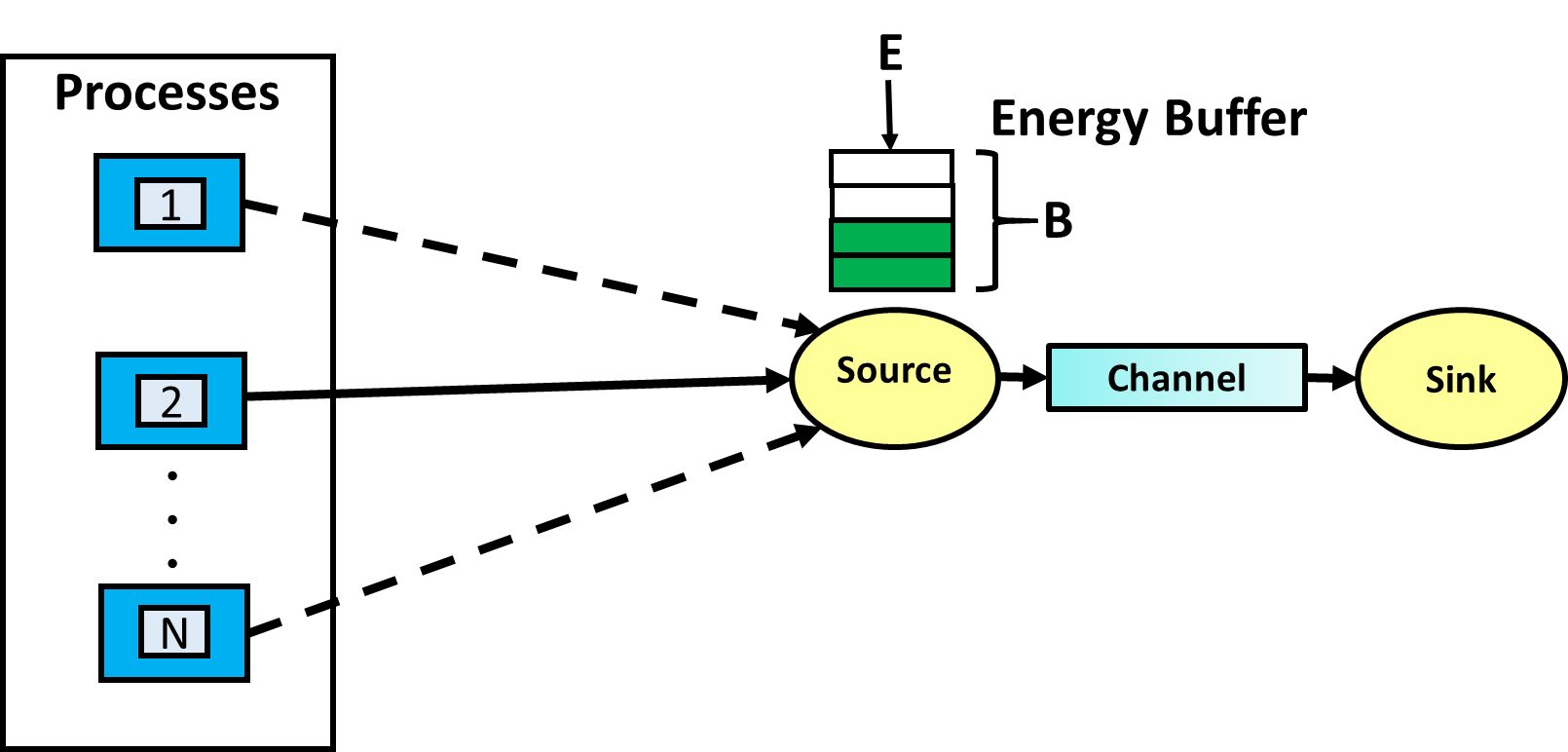
Figure 1: Pictorial representation of a remote sensing system where an EH source samples one of $N$ number of processes at a time and sends the observation packet to a sink node.

However, timely delivery of the status updates is often limited by energy and bandwidth constraints in the network. Recent efforts towards designing EH source nodes (e.g., source nodes equipped with solar panels) have opened a new research paradigm for IoT network operations. The energy generation process in such nodes are very uncertain and typically modeled as a stochastic process. The harvested energy is stored in an energy buffer as energy packets, and used for sensing and communication as and when needed. This EH capability significantly improves network lifetime and eliminates the need for frequent manual battery replacement, but poses a new challenge towards network operations due to uncertainty in the available energy at the source nodes at any given time.

Motivated by the above challenges, we consider the problem of minimizing the time-averaged expected AoI in a remote sensing setting, where a single EH source probes the channel state, samples one or multiple processes and sends the observation packets to the sink node over a fading channel. Energy generation process is modeled as a discrete-time i.i.d. process, and a finite energy buffer is considered. Two variants of the problem are considered: (i) single process with CSIT, (ii) multiple processes with CSIT. Channel state probing and process sampling for time-averaged expected AoI minimization is formulated as an MDP, and the threshold nature of the optimal policy is established analytically for each case. Next, we propose reinforcement learning (RL) algorithms to find the optimal policy when the channel statistics and energy harvesting characteristics are unknown. We also extend these works to the setting where the system has Markovian channel and Markovian energy harvesting process. Numerical results validate the theoretical results and intuitions.

I-A Related work

Initial efforts towards optimizing AoI mostly involved the analysis of various queueing models; e.g., [2] for analysing a single source single server queueing system with FCFS service discipline, [4] for LCFS service discipline for M/M/1 queue, [5] and [6] for multi-source single sink system with M/M/1 queueing at each source, [7] for AoI performance analysis for multi-source single-sink infinite-buffer queueing system where unserved packets are substituted by available newer ones, etc.

On the other hand, a number of papers have considered AoI minimization problem under EH setting: [8] for derivation of average AoI for a single source having finite battery capacity, [9] for derivation of the minimal age policy for EH two hop network, [10] for average AoI expression for single source EH server, [11] for AoI minimization for wirelessly powered user, [12] for sampling, transmission scheduling and transmit power selection for a single source single sink system over infinite time horizon where delay is dependent on the packet transmission energy. The authors in [13] considered two source nodes (power grid node and EH sensor node) sending different data packets to a common destination by using multiple access channel, and derived the delay and AoI of two source nodes respectively.

There have also been several other works on developing optimal scheduling policy for minimizing AoI for EH sensor networks [14, 15, 16, 17, 18, 19, 20, 21, 22, 23, 24]. For example, [14] has investigated optimal online policy for single sensor single sink system with a noiseless channel for infinite, finite and unit size battery capacity; for finite battery size, it has provided energy aware status update policy. The paper [15] has considered a multi-sensor single sink system with infinite battery size, and proposed a randomized myopic scheduling scheme. For an EH source with finite battery and Poisson energy arrival process, the authors in [16] have provided age-energy trade-off and optimal threshold policy for AoI minimization, but unlike our work, they do not consider probing/estimation of a fading channel while making a sampling decision. In [17], the optimal online status update policy to minimize the long run average AoI for EH source with updating erasures have been proposed. It has been shown that the best effort uniform updating policy is optimal when there is no feedback and best-effort uniform updating with re-transmission (BUR) policy is optimal when feedback is available to the source. The authors of [18] examined the problem of minimizing AoI under a constraint on the count of status updates. The authors of [19] addressed AoI minimization problem for cognitive radio communication system with EH capability; they formulated optimal sensing and updating for perfect and imperfect sensing as a partially observable Markov decision process (POMDP). Information source diversity, i.e., multiple sources tracking the same process but with dissimilar energy cost, and sending status updates to the EH monitoring node with finite battery size, has been considered in [20] with an MDP formulation, but no structure was provided for the optimal policy. In [21], reinforcement learning has been used to minimize AoI for a single EH sensor with HARQ protocol, but no clear intuition on the policy structure was provided. In [23], the authors have formulated optimal transmission schemes for an EH sensor which sends update packets to the BS by considering different transmission modes (controlled by power and error probability) and battery recovery setting as an MDP. The authors of [24] have developed a threshold policy for minimizing AoI for a single sensor single sink system with erasure channel and no channel feedback. For a system with Poisson energy arrival, unit battery size and error-free channel, it has shown that a threshold policy achieves average age lower than that of zero-wait policy; based on this, lower bound on average age for general battery size and erasure channel has been derived. The papers [25] and [26] have proposed threshold based sampling policies for AoI minimization in a multi-source system, and also use deep reinforcement learning to learn the optimal policy. However, these paper do not consider channel probing as done in our paper. A very similar claim applies to [27] which also proposes threshold-based scheduling policy.

I-B Our contributions and organization

1. We formulate the problem of minimizing the time-averaged expected AoI in an EH remote sensing system with a single source monitoring one or multiple processes, as an MDP with two stage action model, which is different from standard MDP in the literature. Under the assumptions of i.i.d. time-varying channel with CSIT, channel state probing capability at the source, and finite battery size, we derive the optimal policy structures which turn out to be simple threshold policies. The source node, depending on the current age of a process, decides whether to probe the channel or not. Afterwards, based on the channel probe outcome, the source node decides whether to sample the process and send an observation packet, or to remain idle. Thus, the MDP involves taking action in two stages at each time instant.

2. We prove convergence of an analogue of value iteration for this two-stage MDP.

3. The threshold for multiple processes turns out to be a function of the relative age of the processes.

4. We prove certain interesting properties of various cost functions and some properties of the thresholds as a function of energy and age of the process, either analytically or numerically.

5. We also formulate the AoI minimization problem for a Markovian system as an MDP; the channel dynamics and energy harvesting characteristics are modeled as Markov chains in this case. We provide optimality equations for the MDP. Certain conjectures regarding the threshold structure of the optimal policy for this MDP are validated numerically.

6. For unknown channel statistics and energy harvesting characteristics, we propose reinforcement learning algorithms that yield the optimal policies for the formulated MDPs. However, unlike standard Q-learning algorithm involving a single action at each time instant, we propose a variant of the Q-learning algorithm, that involves taking the action in two stages; first the source decides whether to probe the channel quality, and if the channel quality turns out to be good, then it further decides whether to sample and communicate based on its available energy and age in sampling.

7. We numerically compare the AoI performance of our algorithm with the case where channel probing is not allowed. Surprisingly, it turns out that probing is sometimes better and sometimes worse than no probing; we provide intuitive justification for this, and also assert that channel probing leads to smaller AoI in many practical scenarios.

The rest of the paper is organized as follows. The system model has been explained in Section II. AoI minimization for both single and multiple process case with i.i.d. system model is addressed in Section III, whereas AoI minimization for Markovian system model is considered in Section IV. Further, reinforcement learning for i.i.d. and Markovian system model is proposed in Section V. Lastly, numerical results are provided in Section VI, followed by the conclusions in Section VII. All proofs are provided in the appendices.

II System model

We consider an EH source capable of sensing one out of $N$ different processes at a time, and reporting the observation packet to a sink node over a fading channel; see Figure 1. Time is discretized with the discrete time index $t\in\{0,1,2,3,\cdots\}$. At each time, the source node can decide whether to estimate the quality of the channel from the source to the sink, or not. If the source node decides to probe the channel state, it can further decide whether to sample a process and communicate the data packet to the sink or not, depending on the instantaneous channel quality. The source has a finite energy buffer of size $B$ units, where $E_{p}$ units of buffer energy is used to probe the channel once and $E_{s}$ units of buffer energy is used in sensing and communication of one packet.

II-A Channel model

We consider a fading channel between the source and the sink, where a particular fading state is characterized by the probability of success of a transmitted packet. We denote by $p(t)\in\{p_{1},p_{2},\cdots,p_{m}\}$ the probability of packet transmission success from the source to the sink node at time $t$, and by $C(t)\in\{C_{1},C_{2},\cdots,C_{m}\}$ the corresponding channel state. The packet success probability corresponding to channel state $C_{j}$ is given by $p(C_{j})=p_{j}$. Let us also denote by $r(t)\in\{0,1\}$ the indicator that the packet transmission from the source to the sink at time $t$ is successful. Obviously, $\mathbb{P}(r(t)=1|C(t)=C_{j})=p_{j}$ for all $j\in\{1,2,\cdots,m\}$. It is assumed that the channel state $C(t)$ is learnt perfectly via a channel probe.

I.I.D. channel model: In this case, we assume that $\{p(t)\}_{t\geq 0}$ is i.i.d. across $t$, with $\mathbb{P}(p(t)=p_{j})=q_{j}$ for all $j\in\{1,2,\cdots,m\}$.

Markovian channel model: Here the fading channel is modelled as finite state Markov chain [28], where the one-step state transition probability from state $C_{i}$ to state $C_{j}$ is denoted by $q_{i,j}$ and the $t$-step transition probability is given by $q_{i,j}^{(t)}=P(C(t)=C_{j}|C(0)=C_{i})$ for all $i,j\in\{1,2,\cdots,m\}$.

II-B Energy harvesting process

Let $A(t)$ denote the number of energy packet arrivals to the energy buffer at time $t$, and $E(t)$ denote the energy available to the source at time $t$, for all $t\geq 0$. We consider the following two models for energy harvesting.

I.I.D. model: The energy packet generation process $\{A(t)\}_{t\geq 0}$ in the energy buffer is assumed to be an i.i.d. process with known mean $\lambda>0$.

Markov model: Here the EH state of the source is modelled as a two state Markov chain with states $\{H_{1},H_{2}\}$, where $H_{1}$ is called the harvesting state and $H_{2}$ is called the non harvesting state. When the source node is in harvesting state, the energy packet generation process is considered to be an i.i.d. process with known mean $\lambda>0$. When the source node is in non-harvesting state, then the energy packet generation rate is zero. The transition probability from state $H_{1}$ to state $H_{2}$ is $h_{1,2}$ and from state $H_{2}$ to state $H_{1}$ is $h_{2,1}$. Markov process for energy arrival has previously been used in [29, 30].

We assume that, in case the energy buffer at the source node is full, the newly generated energy packets will not be accommodated unless $E_{p}$ unit of energy is spent in probing.

II-C Decision process and policy

At time $t$, let $b(t)\in\{0,1\}$ denote the indicator of deciding to probe the channel, and $a(t)\in\{0,1,\cdots,N\}$ denote the identity of the process being sampled, with $a(t)=0$ meaning that no process is sampled, and $b(t)=0$ meaning that the channel is not probed. Also, $b(t)=0$ implies $a(t)=0$. The set of possible actions or decisions is denoted by $\mathcal{A}=\{\{0,0\}\cup\{1\times\{0,1,2,\cdots,N\}\}\}$, where a generic action at time $t$ is denoted by $(b(t),a(t))$.

Let us denote by $\tau_{k}(t)\doteq\sup\{0\leq\tau<t:a(\tau)=k,r(\tau)=1\}$ the last time instant before time $t$, when process $k$ was sampled and the observation packet was successfully delivered to the sink. The age of information (AoI) for the $k$-th process at time $t$ is given by $T_{k}(t)=(t-\tau_{k}(t))$. However, if $a(t)=k$ and $r(t)=1$, then $T_{k}(t)=0$ since the current observation of the $k$-th process is available to the sink node. A generic Markov scheduling policy is a collection of mappings $\{\mu_{t}\}_{t\geq 0}$. where $\mu_{t}$ maps $(E(t),C(t),\{T_{k}(t)\}_{1\leq k\leq N})$ to the action space $\mathcal{A}$. If $\mu_{t}=\mu$ for all $t\geq 0$, the policy is called stationary, else non-stationary.

We seek to find a stationary scheduling policy $\mu$ that minimizes the expected sum AoI which is averaged over time:

$$\footnotesize\min_{\mu}\frac{1}{T}\sum_{t=0}^{T}\sum_{k=1}^{N}\mathbb{E}_{\mu}(T_{k}(t))\normalsize$$ (1)

III I.I.D. system

In this section, we derive the optimal channel probing, source activation and data transmission policy for a single EH source sampling a single process ($N=1$) or multiple processes, when the channel and energy harvesting processes follow the i.i.d. model as described in Section II.

III-A Single process ($N=1$)

Here, we formulate (1) as a long-run average cost MDP with state space $\mathcal{S}\doteq\{0,1,\cdots,B\}\times\mathbb{Z}_{+}$ and an intermediate state space $\mathcal{V}=\{0,1,…..,B\}\times\mathbb{Z}_{+}\times\{C_{1},C_{2},\cdots,C_{m}\}$. A generic state $s=(E,T)$ means that the energy buffer has $E$ energy packets, and the source was last activated $T$ slots ago. A generic intermediate state $v=(E,T,C)$ additionally means that the current channel state obtained via probing is $C$. The action space is $\mathcal{A}=\{\{0,0\}\cup\{1\times\{0,1\}\}\}$ with $a(t),b(t)\in\{0,1\}$. At each time, if the source node decides not to probe the channel ($b(t)=0$) and consequently does not sample ($a(t)=0$), the expected single-stage AoI cost is $T$. However, if $b(t)=1$, then the expected single-stage AoI cost is $T$ for $a(t)=0$ and $T(1-p(C))$ for $a(t)=1$, where the expectation of the single stage cost is taken over packet success probability $p(C)$. We first formulate the average-cost MDP problem as an $\alpha$-discounted cost MDP problem with $\alpha\in(0,1)$, and derive the optimal policy, from which the solution of the average cost minimization problem can be obtained by taking $\alpha\rightarrow 1$ [31, Section 4.1].

III-A1 Optimality equation

Let $J^{*}(E,T)$ be the optimal value function for state $(E,T)$ in the discounted cost problem, and let $W^{*}(E,T,C)$ be the cost-to-go from an intermediate state $(E,T,C)$. The Bellman equations are given by:

$$J^{*}(E\geq E_{p}+E_{s},T) = min\bigg{\{}T+\alpha\mathbb{E}_{A}J^{*}(min\{E+A,B\},T+1),$$

$$V^{*}(E,T)\bigg{\}}$$

$$V^{*}(E,T) = \sum_{j=1}^{m}q_{j}W^{*}(E,T,C_{j})$$

$$W^{*}(E,T,C) = min\{T+\alpha\mathbb{E}_{A}J^{*}(min\{E-E_{p}+A,B\},T+1),$$

$$T(1-p(C))+\alpha p(C)\mathbb{E}_{A}J^{*}(min\{E-E_{p}-E_{s}+$$

$$A,B\},1)+\alpha(1-p(C))\mathbb{E}_{A}J^{*}(min\{E-E_{p}-E_{s}+$$

$$A,B\},T+1)\}$$

$$J^{*}(E<E_{p}+E_{s},T) = T+\alpha\mathbb{E}_{A}J^{*}(min\{E+A,B\},T+1)$$ (2)

The first expression in the minimization in the R.H.S. of the first equation in (III-A1) is the cost of not probing channel state ($b(t)=0$), which includes single-stage AoI cost $T$ and an $\alpha$ discounted future cost for a random next state $(min\{E+A,B\},T+1)$, averaged over the distribution of the number of energy packet generation $A$. The quantity $V^{*}(E,T)$ is the expected cost of probing the channel state, which explains the second equation in (III-A1). At an intermediate state $(E,T,C)$, if $a(t)=0$, a single stage AoI cost $T$ is incurred and the next state becomes $(min\{E-E_{p}+A,B\},T+1)$; if $a(t)=1$, the expected AoI cost is $T(1-p(C))$ (expectation taken over the packet success probability $p(C)$), and the next random state becomes $(min\{E-E_{p}-E_{s}+A,B\},1)$ and $(min\{E-E_{p}-E_{s}+A,B\},T+1)$ if $r(t)=1$ and $r(t)=0$, respectively. The last equation in (III-A1) follows similarly since $b(t)=0,a(t)=0$ is the only possible action when $E<E_{p}+E_{s}$.

Substituting the value of $V^{*}(E,T)$ in the first equation of (III-A1), we obtain the following Bellman equations:

$$J^{*}(E\geq E_{p}+E_{s},T)$$ (3)

$$= min\bigg{\{}T+\alpha\mathbb{E}_{A}J^{*}(min\{E+A,B\},T+1),\mathbb{E}_{C}\bigg{(}min\{T+$$

$$\alpha\mathbb{E}_{A}J^{*}(min\{E-E_{p}+A,B\},T+1),T(1-p(C))+$$

$$\alpha p(C)\mathbb{E}_{A}J^{*}(min\{E-E_{p}-E_{s}+A,B\},1)+$$

$$\alpha(1-p(C))\mathbb{E}_{A}J^{*}(min\{E-E_{p}-E_{s}+A,B\},T+1)\}\bigg{)}\bigg{\}}$$

$$J^{*}(E<E_{p}+E_{s},T)$$

$$= T+\alpha\mathbb{E}_{A}J^{*}(min\{E+A,B\},T+1)$$

III-A2 Policy structure

We first provide the convergence proof of value iteration since we have a two-stage decision process as opposed to traditional MDP where a single action is taken.

Proposition 1.

The value function $J^{(t)}(s)$ converges to $J^{*}(s)$ as $t\rightarrow\infty$.

Proof.

See Appendix  A. ∎

Next we provide some properties of the value function, which will help in proving the structure of the optimal policy.

Lemma 1.

For $N=1$, $J^{*}(E,T)$ is increasing in $T$ and $W^{*}(E,T,C)$ is decreasing in $p(C)$.

Proof.

See Appendix  B. ∎

Conjecture 1.

For $N=1$, the optimal probing policy for the $\alpha$-discounted AoI cost minimization problem is a threshold policy on $T$. For any $E\geq E_{p}+E_{s}$, the optimal action is to probe the channel state if and only if $T\geq T_{th}(E)$ for a threshold function $T_{th}(E)$ of $E$.

This conjecture and many other conjectures later have been validated numerically in Section VI.

Theorem 1.

For $N=1$, at any time, if the source decides to probe the channel, then the optimal sampling policy is a threshold policy on $p(C)$. For any $E\geq E_{p}+E_{s}$ and probed channel state, the optimal action is to sample the source node if and only if $p(C)\geq p_{th}(E,T)$ for a threshold function $p_{th}(E,T)$ of $E$ and $T$.

Proof.

See Appendix  C. ∎

The policy structure supports the following two intuitions. Firstly, given $E$ and $T$, the source decides to probe the channel state if AoI is greater than some threshold value. Secondly, given $E$ and $T$ and probed channel state, if the channel quality is better than a threshold, then the optimal action is to sample the process and communicate the observation to the sink node. We will later numerically observe in Section VI some intuitive properties of $T_{th}(E)$ as a function of $E$ and $\lambda$, and $p_{th}(E,T)$ as a function of $E$, $T$ and $\lambda$.

III-A3 No probing case

If we consider the case where the source samples the process directly without channel probing, then the Bellman equations for this case is given by:

$$J^{*}(E\geq E_{s},T) = min\bigg{\{}T+\alpha\mathbb{E}_{A}J^{*}(min\{E+A,B\},T+1),$$

$$\mathbb{E}_{C}\bigg{(}T(1-p(C))+\alpha p(C)\mathbb{E}_{A}J^{*}(min\{E-E_{s}+A,B\},$$

$$1)+\alpha(1-p(C))\mathbb{E}_{A}J^{*}(min\{E-E_{s}+A,B\},T+1)\bigg{)}\bigg{\}}$$

$$J^{*}(E<E_{s},T) = T+\alpha\mathbb{E}_{A}J^{*}(min\{E+A,B\},T+1)$$ (4)

Here also we numerically observe an optimal threshold policy on $T$; see Section VI.

III-B Multiple processes($N>1$)

Here we formulate the $\alpha$-discounted cost version of (1) as an MDP with a generic state $s=(E,T_{1},T_{2},\cdots,T_{N})$ which means that the energy buffer has $E$ energy packets, and the k-th process was last activated $T_{k}$ slots ago. Also, a generic intermediate state is $v=(E,T_{1},T_{2},\cdots,T_{N},C)$ which additionally means that the current channel state $C$ is learnt by probing, has packet success probability $p(C)$. The action space $\mathcal{A}=\{\{0,0\}\cup\{1\times\{0,1,2,\cdots,N\}\}\}$ with $b(t)\in\{0,1\}$ and $a(t)\in\{0,1,\cdots,N\}$. At each time, if the source node decides not to probe the channel state then it will not sample any process, thus $b(t)=0,a(t)=0$ and the expected single stage AoI cost is $\sum_{i=1}^{N}T_{i}$. However, if the source node decides to probe the channel state $(b(t)=1)$, the expected single stage AoI cost is $\sum_{i=1}^{N}T_{i}$ for $a(t)=0$ and $\sum_{i\neq k}T_{i}+T_{k}(1-p(C))$ for $a(t)=k$ where the expectation is taken over packet success probability $p(C)$.

III-B1 Optimality equation

In this case, the Bellman equations are given by:

$$J^{*}(E\geq E_{p}+E_{s},T_{1},T_{2},\cdots,T_{N})$$ (5)

$$= min\bigg{\{}\sum_{i=1}^{N}T_{i}+\alpha\mathbb{E}_{A}J^{*}(min\{E+A,B\},T_{1}+1,T_{2}+1,\cdots,T_{N}+1),$$

$$V^{*}(E,T_{1},T_{2},\cdots,T_{N})\bigg{\}}$$

$$V^{*}(E,T_{1},T_{2},\cdots,T_{N})$$

$$= \sum_{j=1}^{m}q_{j}W^{*}(E,T_{1},T_{2},\cdots,T_{N},C_{j})$$

$$W^{*}(E,T_{1},T_{2},\cdots,T_{N},C)$$

$$= min\{\sum_{i=1}^{N}T_{i}+\alpha\mathbb{E}_{A}J^{*}(min\{E-E_{p}+A,B\},T_{1}+1,T_{2}+1,\cdots,T_{N}+1),$$

$$\min_{1\leq k\leq N}\bigg{(}\sum_{i\neq k}T_{i}+T_{k}(1-p(C))+\alpha p(C)\mathbb{E}_{A}J^{*}(min\{E-E_{p}-E_{s}+A,$$

$$B\},T_{1}+1,T_{2}+1,\cdots,T_{k}^{\prime}=1,T_{k+1}+1,\cdots,T_{N}+1)+\alpha(1-p(C))$$

$$\mathbb{E}_{A}J^{*}(min\{E-E_{p}-E_{s}+A,B\},T_{1}+1,T_{2}+1,\cdots,T_{N}+1)\bigg{)}\}$$

$$J^{*}(E<E_{p}+E_{s},T_{1},T_{2},\cdots,T_{N})$$

$$= \sum_{i=1}^{N}T_{i}+\alpha\mathbb{E}_{A}J^{*}(min\{E+A,B\},T_{1}+1,T_{2}+1,\cdots,T_{N}+1)$$

The first expression in the minimization in the R.H.S. of the first equation in (5) is the cost of not probing channel state ($b(t)=0$), which includes single-stage AoI cost $\sum_{i=1}^{N}T_{i}$ and an $\alpha$ discounted future cost with a random next state $(\min\{E+A,B\},T_{1}+1,T_{2}+1,\cdots,T_{N}+1)$, averaged over the distribution of the number of energy packet generation $A$. The quantity $V^{*}(E,T_{1},T_{2},\cdots,T_{N})$ is the optimal expected cost of probing the channel state, which explains the second equation in (5). At an intermediate state $(E,T_{1},T_{2},\cdots,T_{N},C)$, if $a(t)=0$, a single stage AoI cost $\sum_{i=1}^{N}T_{i}$ is incurred and the next state becomes $(\min\{E-E_{p}+A,B\},T_{1}+1,T_{2}+1,\cdots,T_{N}+1)$; if $a(t)=k$, the expected AoI cost is $\sum_{i\neq k}T_{i}+T_{k}(1-p(C))$ (expectation taken over the packet success probability $p(C)$), and the next random state becomes $(\min\{E-E_{p}-E_{s}+A,B\},T_{1}+1,T_{2}+1,\cdots,T_{k}^{\prime}=1,T_{k+1}+1,\cdots,T_{N}+1)$ and $(\min\{E-E_{p}-E_{s}+A,B\},T_{1}+1,T_{2}+1,\cdots,T_{N}+1)$ if $r(t)=1$ and $r(t)=0$, respectively. The last equation in (5) follows similarly since $b(t)=0,a(t)=0$ is the only possible action when $E<E_{p}+E_{s}$.

Substituting the value of $V^{*}(E,T_{1},T_{2},\cdots,T_{N})$ in the first equation of (5), we obtain the Bellman equations (III-B1).

$$J^{*}(E\geq E_{p}+E_{s},T_{1},T_{2},\cdots,T_{N}) = min\bigg{\{}\sum_{i=1}^{N}T_{i}+\alpha\mathbb{E}_{A}J^{*}(min\{E+A,B\},T_{1}+1,T_{2}+1,\cdots,T_{N}+1),$$

$$\mathbb{E}_{C}\bigg{(}min\{\sum_{i=1}^{N}T_{i}+\alpha\mathbb{E}_{A}J^{*}(min\{E-E_{p}+A,B\},T_{1}+1,T_{2}+1,\cdots,T_{N}+1),$$

$$\min_{1\leq k\leq N}\bigg{(}\sum_{i\neq k}T_{i}+T_{k}(1-p(C))+\alpha p(C)\mathbb{E}_{A}J^{*}(min\{E-E_{p}-E_{s}+A,B\},T_{1}+1,$$

$$T_{2}+1,\cdots,T_{k}^{\prime}=1,T_{k+1}+1,\cdots,T_{N}+1)+\alpha(1-p(C))\mathbb{E}_{A}J^{*}(min\{E-E_{p}-E_{s}+A,B\},$$

$$T_{1}+1,T_{2}+1,\cdots,T_{N}+1)\bigg{)}\}\bigg{)}\bigg{\}}$$

$$J^{*}(E<E_{p}+E_{s},T_{1},T_{2},\cdots,T_{N}) = \sum_{i=1}^{N}T_{i}+\alpha\mathbb{E}_{A}J^{*}(min\{E+A,B\},T_{1}+1,T_{2}+1,\cdots,T_{N}+1)$$ (6)

 

III-B2 Policy structure

Lemma 2.

For $N>1$, the value function $J^{*}(E,T_{1},T_{2},\cdots,T_{N})$ is increasing in each of $T_{1},T_{2},\cdots,T_{N}$ and $W^{*}(E,T_{1},T_{2},\cdots,T_{N},C)$ is decreasing in $p(C)$.

Proof.

See Appendix  D. ∎

Let us define $\bm{T}=[T_{1},T_{2},\cdots,T_{N}]$ and $\bm{T}_{-k}=[T_{1},T_{2},\cdots,T_{k-1},T_{k+1},\cdots,T_{N}]$.

Conjecture 2.

For $N>1$, the optimal probing policy for the $\alpha$-discounted AoI cost minimization problem is a threshold policy on $\max_{1\leq k\leq N}T_{k}\doteq T_{k^{*}}$. For any $E\geq E_{p}+E_{s}$, the optimal action is to probe the channel state if and only if $\max_{1\leq k\leq N}T_{k}\geq T_{th}(E,\bm{T}_{-k^{*}})$ for a threshold function $T_{th}(E,\bm{T}_{-k^{*}})$ of $E$ and $\bm{T}_{-k^{*}}$.

We next show that sampling the process with largest AoI is optimal.

Theorem 2.

For $N>1$, after probing the channel state, the optimal source activation policy for the $\alpha$-discounted cost problem is a threshold policy on p(C). For any $E\geq E_{p}+E_{s}$ and probed channel state, the optimal action is to sample the process $\arg\max_{1\leq k\leq N}T_{k}$ if and only if $p(C)\geq p_{th}(E,\bm{T})$ for a threshold function $p_{th}(E,\bm{T})$ of $(E,\bm{T})$.

Proof.

See Appendix  E. ∎

We will later numerically demonstrate some intuitive properties of $T_{th}(E,\bm{T}_{-k})$ as a function of $E$, $\bm{T}_{-k}$ and $\lambda$ and $p_{th}(E,T_{1},T_{2},\cdots,T_{N})$ as a function of $E$, $(T_{1},T_{2},\cdots,T_{N})$ and $\lambda$ in Section VI.

IV Markovian System Model: single process

Here, we derive the optimal channel probing, source activation and data transmission policy for an EH source sampling a single process with Markovian channel and Markovian energy arrival process. We formulate the $\alpha$-discounted cost version of (1) as an MDP with state space $\mathcal{S}\doteq\{0,1,\cdots,B\}\times\mathbb{Z}_{+}\times\mathbb{Z}_{+}\times\{C_{1},C_{2},\cdots,C_{m}\}\times\{H_{1},H_{2}\}$ where a generic state $s=(E,T,\tau,C_{prev},H_{1})$ means that the energy buffer has $E$ energy packets, the source was last activated $T$ slots ago, the channel state was last probed $\tau$ slots ago where $\tau\leq T$, the previous channel state obtained via probing is $C_{prev}\in\{C_{1},C_{2},\cdots,C_{m}\}$, and the EH source is in harvesting state $H_{1}$. A generic state $s=(E,T,\tau,C_{prev},H_{2})$ similarly means that the EH source is in non-harvesting state $H_{2}$. Also, $\mathcal{V}$ denotes intermediate state space where a generic state $v=(E,T,C,H_{1})$ or $v=(E,T,C,H_{2})$ is used for current channel state $C$ (obtained after probing). The action space $\mathcal{A}=\{\{0,0\}\cup\{1\times\{0,1\}\}\}$ with $a(t),b(t)\in\{0,1\}$. At each time, if $b(t)=0,a(t)=0$, then the expected single-stage AoI cost is $T$. However, if $b(t)=1$, the expected single-stage AoI cost is $T$ and $T(1-p(C))$ for $a(t)=0$ and $a(t)=1$, respectively.

IV-A Optimality equation

In this case, for state $(E,T,\tau,C_{prev},H_{1})$, the Bellman equations are given by:

$$J^{*}(E\geq E_{p}+E_{s},T,\tau,C_{prev},H_{1})$$

$$= min\bigg{\{}T+\alpha\mathbb{E}_{A|H_{1},H_{next}|H_{1}}J^{*}(min\{E+A,B\},T+1,\tau+1,C_{prev},$$

$$H_{next}),V^{*}(E,T,\tau,C_{prev},H_{1})\bigg{\}}$$

$$V^{*}(E,T,\tau,C_{prev},H_{1})$$

$$= \mathbb{E}_{C\sim q^{(\tau)}(\cdot|C_{prev})}W^{*}(E,T,C,H_{1})$$

$$W^{*}(E,T,C,H_{1})$$

$$= min\{T+\alpha\mathbb{E}_{A|H_{1},H_{next}|H_{1}}J^{*}(min\{E-E_{p}+A,B\},T+1,1,C,$$

$$H_{next}),T(1-p(C))+\alpha p(C)\mathbb{E}_{A|H_{1},H_{next}|H_{1}}J^{*}(min\{E-E_{p}-$$

$$E_{s}+A,B\},1,1,C,H_{next})+\alpha(1-p(C))\mathbb{E}_{A|H_{1},H_{next}|H_{1}}J^{*}(min$$

$$\{E-E_{p}-E_{s}+A,B\},T+1,1,C,H_{next})\}$$

$$J^{*}(E<E_{p}+E_{s},T,\tau,C_{prev},H_{1})$$

$$= T+\alpha\mathbb{E}_{A|H_{1},H_{next}|H_{1}}J^{*}(min\{E+A,B\},T+1,\tau+1,C_{prev},H_{next})$$

The first expression in the minimization in the R.H.S. of the first equation in (IV-A) is the cost when $b(t)=0$. The quantity $V^{*}(E,T,\tau,C_{prev},H_{1})$ is the expected cost when $b(t)=1$, which explains the second equation in (IV-A). Here $q^{(\tau)}$ denote the $\tau$-step transition probability of the channel dynamics, starting from $C_{prev}$.

Similarly, in (IV-A), if we consider $H_{2}$ for state $(E,T,\tau,C_{prev},H_{2})$ then the same Bellman equations hold with $A=0$.

IV-B Policy structure

We conjecture the following properties regarding the value function and the optimal policy. Numerical validation of these conjectures is given in VI-C.

Conjecture 3.

For Markovian system model and $N=1$, the value function $J^{*}(E,T,\tau,C_{prev},H)$ is increasing in $T$ and $W^{*}(E,T,C,H)$ is decreasing in $p(C)$.

Conjecture 4.

For Markovian system model and $N=1$, the optimal probing policy for the $\alpha$-discounted AoI cost minimization problem is a threshold policy on $T$. For any $E\geq E_{p}+E_{s}$, the optimal action is to probe the channel state if and only if $T\geq T_{th}(E,\tau,C_{prev},H)$ for a threshold function $T_{th}(E,\tau,C_{prev},H)$ of $E,\tau,C_{prev},H$.

Conjecture 5.

For Markovian system model and $N=1$, at any time, if the source decides to probe the channel, then the optimal sampling policy is a threshold policy on $p(C)$. For any $E\geq E_{p}+E_{s}$ and probed channel state, the optimal action is to sample the source node if and only if $p(C)\geq p_{th}(E,T,H)$ for a threshold function $p_{th}(E,T,H)$ of $E$, $T$ and $H$.

V Reinforcement Learning for AoI Optimization: Single Process

If the channel statistics and the energy harvesting characteristics are not known at the source, then the source has to learn them with time. We adapt the Q-learning technique [32, Section 11.4.2] to find the optimal policy for our two-stage action model.

V-A I.I.D. system

Here we assume that the energy generation rate $\lambda$ and the channel state probabilities $\{q_{j}\}_{1\leq j\leq m}$ are not known to the source. The packet success probabilities $\{p_{j}\}_{1\leq j\leq m}$ are either known or unknown; the packet success indicator $r(t)$ is used to estimate $p_{j}$ if it is unknown.

V-A1 Optimality equation in terms of Q-function

The optimal Q function is denoted by $Q^{*}(E,T,b)$ for a generic state-action pair $(E,T,b)$, where the state is $(E,T)$ and the action is $b\in\{0,1\}$. The quantity $Q^{*}(E,T,b)$ denotes the expected cost obtained if the current state is $(E,T)$, current action chosen is $b$, and an optimal policy is employed from the next time instant. Also, $Q^{*}(E,T,C,a)$ corresponds to the intermediate state $(E,T,C)$ and a corresponding action $a\in\{0,1\}$. It is important to note that, we have to maintain two different types of Q functions to handle states and intermediate states; this is not done in standard Q-learning. The optimal Q-value functions are given by:

$$Q^{*}(E\geq E_{p}+E_{s},T,b=0)$$ (8)

$$= T+\alpha\mathbb{E}_{A}J^{*}(min\{E+A,B\},T+1)$$

$$= T+\alpha\mathbb{E}_{A}\min_{b\in\{0,1\}}Q^{*}(min\{E+A,B\},T+1,b)$$

Here the terms in the R.H.S of the first equality operator in (8) is the immediate cost of not probing channel state action $(b=0)$ when state is $(E\geq E_{p}+E_{s},T)$ and an $\alpha$ discounted future cost $\mathbb{E}_{A}J^{*}(min\{E+A,B\},T+1)$ which is later substituted by $\mathbb{E}_{A}\min_{b\in\{0,1\}}Q^{*}(min\{E+A,B\},T+1,b)$ (averaged over the distribution of A). On the other hand,

$$Q^{*}(E\geq E_{p}+E_{s},T,b=1) = \sum_{j=1}^{m}q_{j}W^{*}(E,T,C_{j})$$ (9)

$$= \sum_{j=1}^{m}q_{j}\min_{a\in\{0,1\}}Q^{*}(E,T,C_{j},a)$$

Now,

$$Q^{*}(E,T,C,a=0)$$ (10)

$$= T+\alpha\mathbb{E}_{A}\underbrace{\min_{b\in\{0,1\}}Q^{*}(min\{E-E_{p}+A,B\},T+1,b)}_{=J^{*}(min\{E-E_{p}+A,B\},T+1)}$$

and

$$Q^{*}(E,T,C,a=1)$$

$$= T(1-p(C))+\alpha p(C)\mathbb{E}_{A}\min_{b\in\{0,1\}}Q^{*}(min\{E-E_{p}-E_{s}+A,B\},1,b)$$

$$+\alpha(1-p(C))\mathbb{E}_{A}\min_{b\in\{0,1\}}Q^{*}(min\{E-E_{p}-E_{s}+A,B\},T+1,b)$$

Similarly, the optimal Q-function for state $(E<E_{p}+E_{s},T)$ is given by (12) in which only not probing $(b=0)$ is a feasible action:

$$Q^{*}(E<E_{p}+E_{s},T,b=0)$$ (12)

$$= T+\alpha\mathbb{E}_{A}J^{*}(min\{E+A,B\},T+1)$$

$$= T+\alpha\mathbb{E}_{A}\min_{b\in\{0,1\}}Q^{*}(min\{E+A,B\},T+1,b)$$

V-A2 Q-Learning algorithm

The optimal Q function is given by the zeros of (8)-(12). Here, we employ asynchronous stochastic approximation [33] to iteratively converge to the optimal Q function, starting from any arbitrary Q-function. Online learning is facilitated by sequentially observing $C(t)$ (via channel probing), $r(t)$ (via transmission ACK/NACK) and the number $A(t)$ of energy packets harvested at time $t$.

In asynchronous stochastic approximation, we need step size sequence $d(t)$ ($t\geq 0$) which satisfies the following assumptions [34]:

Assumption 1.

(i) $0<d(t)\leq\bar{d}$ where $\bar{d}>0$,
(ii) $d(t+1)\leq d(t)$ for all $t\geq 0$,
(iii) $\sum_{t=0}^{\infty}d(t)=\infty$ and $\sum_{t=0}^{\infty}(d(t))^{2}<\infty$.

Let us denote by $\nu_{t}(s,b)$ the number of occurrences of the state-action pair $(s,b)$ up to iteration $t$ where $s\in\mathcal{S}$ and $b\in\{0,1\}$. A similar notation is assumed for any generic intermediate state $v$ and the corresponding action $a$. The following assumption is required for the convergence of asynchronous stochastic approximation [34].

Assumption 2.

$\lim\inf_{t\rightarrow\infty}\frac{\nu_{t}(s,b)}{t}>0$ almost surely $\forall(s,b)$, and $\lim\inf_{t\rightarrow\infty}\frac{\nu_{t}(v,a)}{t}>0$ almost surely $\forall(v,a)$.

The proposed algorithm maintains a look-up table $Q_{t}(\cdot,\cdot)$ for various state-action pairs, and iteratively updates its entries depending on the current state, current action taken and the observed next state. However, Assumption 2 requires that all state-action pairs should be visited infinitely and comparatively often. This is ensured by taking a random action (uniformly chosen) with probability $\epsilon$ at each decision instant, and taking the action $\arg min_{b}Q(s,b)$ or $\arg min_{a}Q(v,a)$ with probability $(1-\epsilon)$.

One example of Q-value update is the following, aimed at convergence to the solution of (8):

$$Q_{t+1}(E\geq E_{p}+E_{s},T,b=0)$$ (13)

$$= Q_{t}(E,T,b=0)+d(\nu_{t}(E,T,b=0))\mathrm{\mathbf{1}}\{s(t)=(E,T),b(t)=0\}[T$$

$$+\alpha\min_{b\in\{0,1\}}Q_{t}(min\{E+A(t),B\},T+1,b)-Q_{t}(E,T,b=0)]$$

Here $\mathrm{\mathbf{1}}\{\cdot\}$ is the indicator function. It is important to note that, this $Q$ update can be performed only when the random next state $(min\{E+A(t),B\},T+1)$ is is observed.

In a similar fashion, equations (9)-(12) lead to the following Q-updates for various states and intermediate states:

$$Q_{t+1}(E\geq E_{p}+E_{s},T,b=1)$$ (14)

$$= Q_{t}(E,T,b=1)+d(\nu_{t}(E,T,b=1)\mathrm{\mathbf{1}}\{s(t)=(E,T),b(t)=1\}$$

$$[\min_{a\in\{0,1\}}Q_{t}(E,T,C,a)-Q_{t}(E,T,b=1)]$$

$$Q_{t+1}(E,T,C,a=0)$$ (15)

$$= Q_{t}(E,T,C,a=0)+d(\nu_{t}(E,T,C,a=0))\mathrm{\mathbf{1}}\{v(t)=(E,T,C),$$

$$a(t)=0\}[T+\alpha\min_{b\in\{0,1\}}Q_{t}(min\{E-E_{p}+A(t),B\},T+1,b)$$

$$-Q_{t}(E,T,C,a=0)]$$

$$Q_{t+1}(E,T,C,a=1)$$ (16)

$$= Q_{t}(E,T,C,a=1)+d(\nu_{t}(E,T,C,a=1))\mathrm{\mathbf{1}}\{v(t)=(E,T,C),$$

$$a(t)=1\}[T(1-p(C))+\alpha p(C)\min_{b\in\{0,1\}}Q_{t}(min\{E-E_{p}-E_{s}+A(t),$$

$$B\},1,b)+\alpha(1-p(C))\min_{b\in\{0,1\}}Q_{t}(min\{E-E_{p}-E_{s}+A(t),B\},T+1,$$

$$b)-Q_{t}(E,T,C,a=1)]$$

$$Q_{t+1}(E<E_{p}+E_{s},T,b=0)$$ (17)

$$= Q_{t}(E,T,b=0)+d(\nu_{t}(E,T,b=0))\mathrm{\mathbf{1}}\{s(t)=(E,T),b(t)=0\}[T+$$

$$\alpha\min_{b\in\{0,1\}}Q_{t}(min\{E+A(t),B\},T+1,b)-Q_{t}(E,T,b=0)]$$

In (16), we consider the case where packet success probability $p(C)$ for channel state $C$ is known to the source. However, if these probabilities are unknown, then one can replace $p(C)$ in (16) by $r(t)$ to obtain a valid Q-update.

Q learning type algorithm for $N>1$ can also be formulated similarly.

V-B Markovian system

Here we adapt Q-learning for the Markovian model with unknown channel statistics and unknown energy harvesting characteristics to obtain the optimal solutions for (IV-A).

V-B1 Optimality equation in terms of Q-function

The optimal Q-value functions are given by:

$$Q^{*}(E\geq E_{p}+E_{s},T,\tau,C_{prev},H_{1},b=0)$$ (18)

$$= T+\alpha\mathbb{E}_{A|H_{1},H_{next}|H_{1}}J^{*}(min\{E+A,B\},T+1,\tau+1,C_{prev},$$

$$H_{next})$$

$$= T+\alpha\mathbb{E}_{A|H_{1},H_{next}|H_{1}}\min_{b\in\{0,1\}}Q^{*}(min\{E+A,B\},T+1,\tau+1,$$

$$C_{prev},H_{next},b)$$

On the other hand,

$$Q^{*}(E\geq E_{p}+E_{s},T,\tau,C_{prev},H_{1},b=1)$$ (19)

$$= \mathbb{E}_{C\sim q^{(\tau)}(\cdot|C_{prev})}W^{*}(E,T,C,H_{1})$$

$$= \mathbb{E}_{C\sim q^{(\tau)}(\cdot|C_{prev})}\min_{a\in\{0,1\}}Q^{*}(E,T,C,H_{1},a)$$

When $b(t)=1$, for a current measured channel state $C$, the optimal ${Q}^{*}$ functions for action $a=0$ and $a=1$ are given by:

$${Q}^{*}(E,T,C,H_{1},a=0)$$ (20)

$$= T+\alpha\mathbb{E}_{A|H_{1},H_{next}|H_{1}}\min_{b\in\{0,1\}}Q^{*}(min\{E-E_{p}+A,B\},T+1,$$

$$1,C,H_{next},b)$$

$${Q}^{*}(E,T,C,H_{1},a=1)$$ (21)

$$= T(1-p(C))+\alpha p(C)\mathbb{E}_{A|H_{1},H_{next}|H_{1}}\min_{b\in\{0,1\}}Q^{*}(min\{E-E_{p}-E_{s}$$

$$+A,B\},1,1,C,H_{next},b)+\alpha(1-p(C))\mathbb{E}_{A|H_{1},H_{next}|H_{1}}\min_{b\in\{0,1\}}$$

$$Q^{*}(min\{E-E_{p}-E_{s}+A,B\},T+1,1,C,H_{next},b)\}$$

Also, the optimal Q-function for state $(E<E_{p}+E_{s},T,\tau,C_{prev},H_{1})$ is given by:

$$Q^{*}(E<E_{p}+E_{s},T,\tau,C_{prev},H_{1},b=0)$$ (22)

$$= T+\alpha\mathbb{E}_{A|H_{1},H_{next}|H_{1}}\min_{b\in\{0,1\}}Q^{*}(min\{E+A,B\},T+1,\tau+1,$$

$$C_{prev},H_{next},b)$$

Similarly, the Q functions are given for state $(E,T,\tau,C_{prev},H_{2})$ by putting $A=0$.

V-B2 Q-Learning algorithm

Here also we employ asynchronous stochastic approximation to find the solution of (18)-(22) as in V-A. The Q-updates for various states and intermediate states are given by following:

$$Q_{t+1}(E\geq E_{p}+E_{s},T,\tau,C_{prev},H_{1},b=0)$$ (23)

$$= Q_{t}(E,T,\tau,C_{prev},H_{1},b=0)+d(\nu_{t}(E,T,\tau,C_{prev},H_{1},b=0))$$

$$\mathrm{\mathbf{1}}\{s(t)=(E,T,\tau,C_{prev},H_{1}),b(t)=0\}[T+\alpha\min_{b\in\{0,1\}}Q_{t}(min\{E+A(t),$$

$$B\},T+1,\tau+1,C_{prev},H_{next},b)-Q_{t}(E,T,\tau,C_{prev},H_{1},b=0)]$$

$$Q_{t+1}(E\geq E_{p}+E_{s},T,\tau,C_{prev},H_{1},b=1)$$ (24)

$$= Q_{t}(E,T,\tau,C_{prev},H_{1},b=1)+d(\nu_{t}(E,T,\tau,C_{prev},H_{1},b=1))$$

$$\mathrm{\mathbf{1}}\{s(t)=(E,T,\tau,C_{prev},H_{1}),b(t)=1\}[\min_{a\in\{0,1\}}Q_{t}(E,T,C,H_{1},a)-$$

$$Q_{t}(E,T,\tau,C_{prev},H_{1},b=1)]$$

$$Q_{t+1}(E,T,C,H_{1},a=0)$$ (25)

$$= Q_{t}(E,T,C,H_{1},a=0)+d(\nu_{t}(E,T,C,H_{1},a=0))\mathrm{\mathbf{1}}\{v(t)=$$

$$(E,T,C,H_{1}),a(t)=0\}[T+\alpha\min_{b\in\{0,1\}}Q_{t}(min\{E-E_{p}+A(t),B\},$$

$$T+1,1,C,H_{next},b)-Q_{t}(E,T,C,H_{1},a=0)]$$

$$Q_{t+1}(E,T,C,H_{1},a=1)$$

$$= Q_{t}(E,T,C,H_{1},a=1)+d(\nu_{t}(E,T,C,H_{1},a=1))\mathrm{\mathbf{1}}\{v(t)=$$

$$(E,T,C,H_{1}),a(t)=1\}[T(1-p(C))+\alpha p(C)\min_{b\in\{0,1\}}Q_{t}(min\{E-$$

$$E_{p}-E_{s}+A(t),B\},1,1,C,H_{next},b)+\alpha(1-p(C))\min_{b\in\{0,1\}}Q_{t}(min\{E$$

$$-E_{p}-E_{s}+A(t),B\},T+1,1,C,H_{next},b)-Q_{t}(E,T,C,H_{1},a=1)]$$

$$Q_{t+1}(E<E_{p}+E_{s},T,\tau,C_{prev},H_{1},b=0)$$

$$= Q_{t}(E,T,\tau,C_{prev},H_{1},b=0)+d(\nu_{t}(E,T,\tau,C_{prev},H_{1},b=0))$$

$$\mathrm{\mathbf{1}}\{s(t)=(E,T,\tau,C_{prev},H_{1}),b(t)=0\}[T+\alpha\min_{b\in\{0,1\}}Q_{t}(min\{E+A(t),$$

$$B\},T+1,\tau+1,C_{prev},H_{next},b)-Q_{t}(E,T,\tau,C_{prev},H_{1},b=0)]$$

Similarly, the Q-value function iteration updates are given for state $(E,T,\tau,C_{prev},H_{2})$ by taking $A=0$. Also, when $p(C)$ is not known, it can be replaced by $r(t)$ in (V-B2).

VI Numerical results

VI-A Single process, I.I.D. system, known dynamics

We consider five channel states ($m=5$) with channel state occurrence probabilities $\bm{q}=[0.2,0.2,0.2,0.2,0.2]$ and the corresponding packet success probabilities $\bm{p}=[0.9,0.7,0.5,0.3,0.1]$. Energy arrival process is i.i.d. $Bernoulli(\lambda)$ with energy buffer size $B=12$, $E_{p}=1$ unit, $E_{s}=1$ unit. Numerical exploration reveals that there exists a threshold policy on $T$ in decision making for channel state probing; see Figure  2(a) which substantiates our conjecture in III-A2. It is observed that this $T_{th}(E)$ decreases with $E$ since higher available energy in the energy buffer allows the EH node to probe the channel state more aggressively. Similar reasoning explains the observation that $T_{th}(E)$ decreases with $\lambda$. For probed channel state, Figure 2(b) shows the variation of $p_{th}(E,T)$ with $E,T,\lambda$. It is observed that $p_{th}(E,T)$ decreases with $E$, since the EH node tries to sample the process more aggressively if more energy is available in the buffer. Similarly, higher value of $T$ results in aggressive sampling, and hence $p_{th}(E,T)$ decreases with $T$. By similar arguments as before, we can explain the observation that this $p_{th}(E,T)$ decreases with $\lambda$.

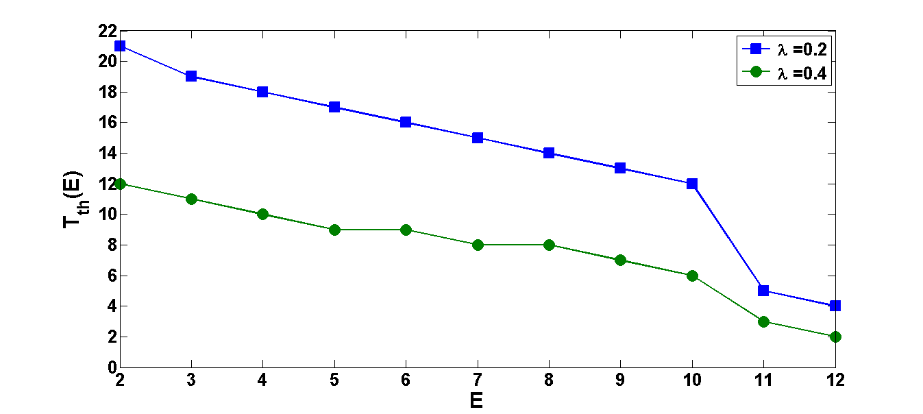
(a)

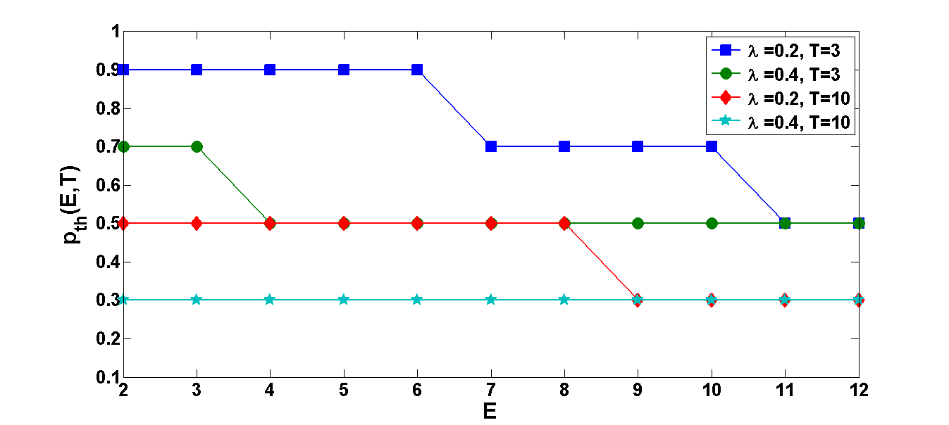
(b)

Figure 2: Single process ($N=1$), I.I.D. model, known dynamics: (a) Variation of $T_{th}(E)$ with $E,\lambda$ and (b) Variation of $p_{th}(E,T)$ with $E,T,\lambda$.

VI-B Multiple processes ($N>1$), I.I.D. model, known dynamics

We choose $N=3,B=12,E_{p}=1,E_{s}=1$ and the same channel model and parameters as in Section VI-A. Figure 3(a) provides validation to our conjecture for optimal probing policy in III-B2 by demonstrating the variation on the threshold on $T_{1}$ for given $T_{2},T_{3}$, for channel state probing. It is observed that $T_{th}(E,T_{2},T_{3})$ decreases with $E$ and $\lambda$. Extensive numerical work also demonstrated that this threshold decreases with each of $T_{2}$, $T_{3}$. For probed channel state, Figure 3(b) shows that $p_{th}(E,T_{1},T_{2},T_{3})$ decreases with $E$ and $\lambda$. Further numerical analysis also demonstrated that this threshold decreases with each of $T_{1}$, $T_{2}$, $T_{3}$ .

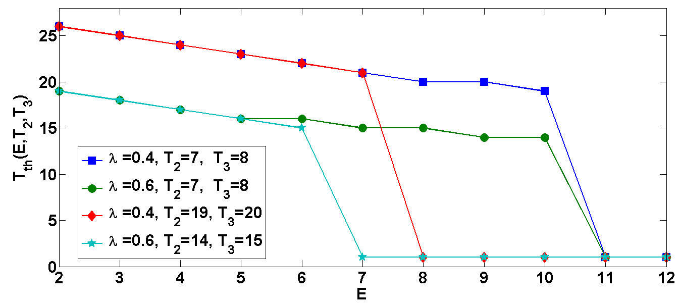
(a)

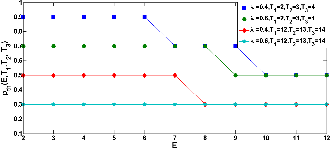
(b)

Figure 3: $N=3$, I.I.D. model, known dynamics: (a) Variation of $T_{th}(E,T_{2},T_{3})$ with $E,T_{2},T_{3},\lambda$ and (b) Variation of $p_{th}(E,T_{1},T_{2},T_{3})$ with $E,T_{1},T_{2},T_{3},\lambda$.

VI-C Markovian model, $N=1$, known dynamics

We consider a two state Markovian fading channel ($m=2$), where $C_{1}$ is the good channel state and $C_{2}$ is the bad channel state. The channel state transition probabilities are $q_{1,2}=0.1$ and $q_{2,1}=0.1$, and the corresponding packet transmission success probabilities are $p_{1}=0.9,p_{2}=0.4$. Also, for the Markovian energy harvesting process, we consider the transition probabilities $h_{1,2}=0.3$ and $h_{2,1}=0.3$. When the source node is in harvesting state, the energy packet generation process is i.i.d. $Bernoulli(\lambda)$ across time, and otherwise zero. We consider $B=9$, $E_{p}=1$ unit, $E_{s}=1$ unit, and $\lambda=0.4$.

Our numerical exploration demonstrated the threshold nature of the optimal policy which verified conjectures predicted in IV-B. Figure 4 shows that, for a fixed $\tau$, $T_{th}(E,\tau,C_{prev},H)$ decreases with $E$, $T_{th}(E,\tau,C_{prev},H_{1})\leq T_{th}(E,\tau,C_{prev},H_{2})$ and $T_{th}(E,\tau,C_{1},H)\leq T_{th}(E,\tau,C_{2},H)$ (because probability of packet success in channel state $C_{1}$ is higher than that in $C_{2}$). Also, from Figure 5(a) it is observed that for probed channel state, $p_{th}(E,T,H)$ decreases with $E$ and $T$, and $p_{th}(E,T,H_{1})\leq p_{th}(E,T,H_{2})$.

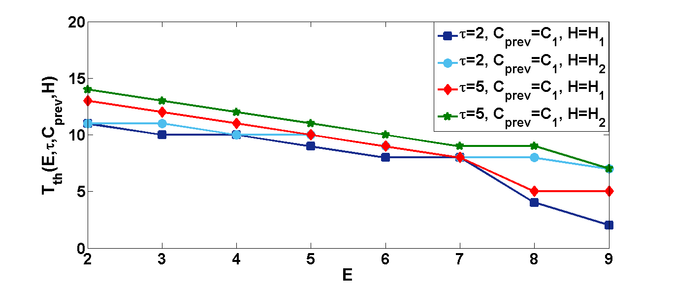
(a)

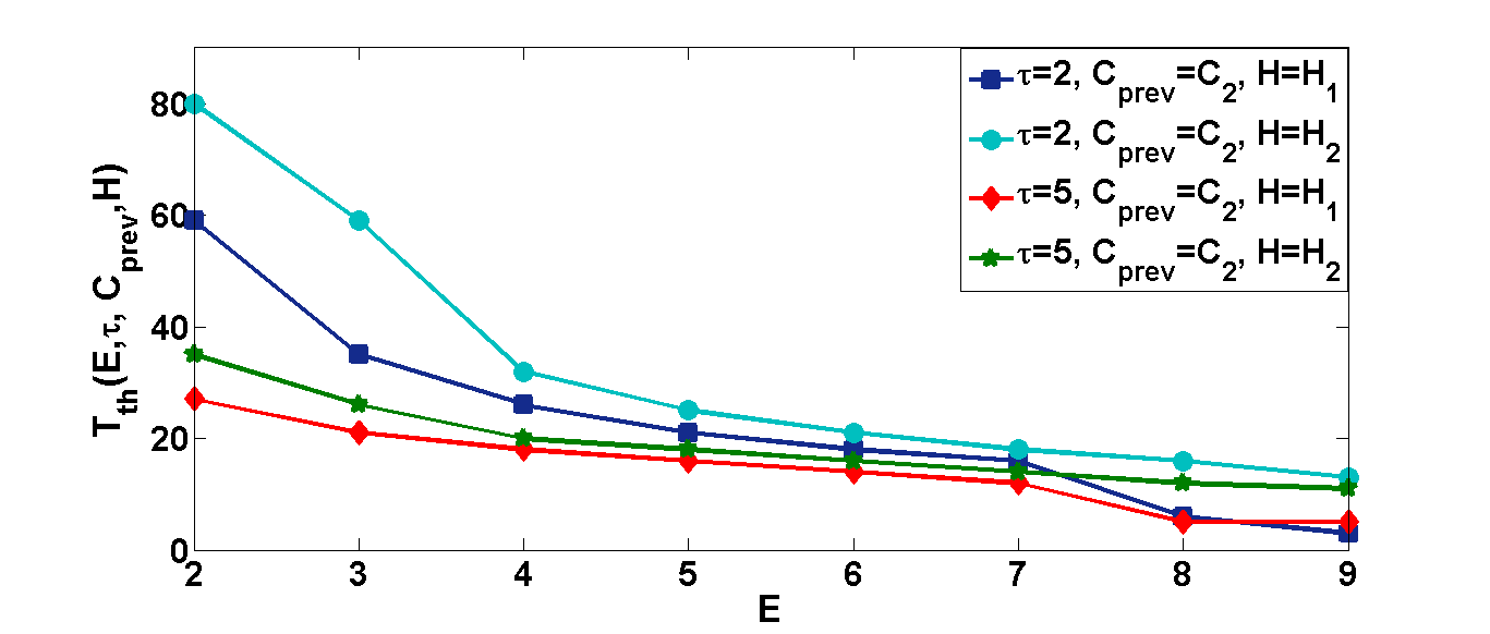
(b)

Figure 4: $N=1$, Markov model: (a) Variation of $T_{th}(E,\tau,C_{prev},H)$ with $E$, $\tau$, $C_{prev}=C_{1}$ and $H$ and (b) Variation of $T_{th}(E,\tau,C_{prev},H)$ with $E$, $\tau$, $C_{prev}=C_{2}$ and $H$.

Also, numerical exploration revealed that, after probing is done, the optimal sampling policy can also be represented as a threshold policy on $T$ instead of $p(C)$; in this case, sampling is done when $T\geq T_{th}(E,C,H)$. The variation of $T_{th}(E,C,H)$ with $E,C,H$ is shown in Figure  5(b), which supports many intuitive justifications provided earlier in this section.

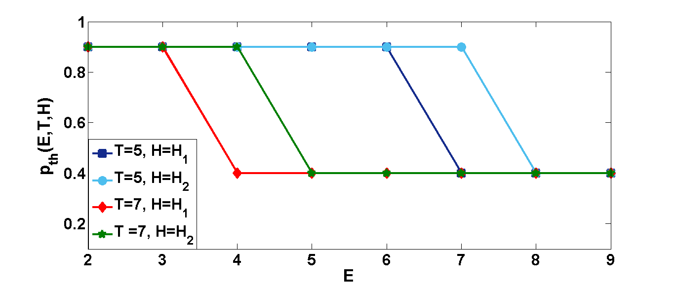
(a)

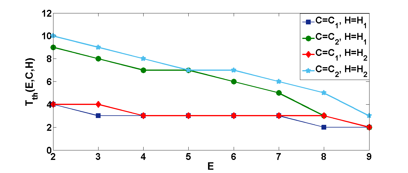
(b)

Figure 5: $N=1$, Markov model: (a) Variation of $p_{th}(E,T,H)$ with $E$, $T$, and $H$ (b) Variation of $T_{th}(E,C,H)$ with $E$, $C$, and $H$.

VI-D Comparison between probing and not probing

VI-D1 I.I.D. System

We consider $N=1$ and the same model as in Section VI-A, and compare the performance of our probing based threshold policy against the optimal policy that involves sampling mandatorily without probing (as in Section III-A3) based on $T$ and $E$. The results are summarised in Figure 6 (a); we note that AoI increases with $E_{p}$ and $E_{s}$ since each action becomes more costly for the source. One interesting observation is that when the sensing energy is close to probing energy ($E_{s}=1,E_{p}=1$), we see slightly higher time averaged AoI values for probing case compared to the case with $E_{s}=1$ and no probing. This happens because the advantage offered by probing is being overshadowed by the extra amount of energy expended for it. However, when $E_{s}=5,E_{p}=1$, we notice that probing yields a lower time averaged AoI. Obviously, the importance of probing is dependent on the trade off between the advantage offered by probing and the extra energy required for it. Typically, $E_{p}$ is much smaller than $E_{s}$ since probing requires less energy as compared to sampling and transmitting a data packet. We have also observed numerically that, when there is sufficient variation in the channel quality, probing improves the AoI performance. On the other hand, when channel variation is not predominant, spending energy in probing tends to hit the AoI performance and can sometimes render it worse than no probing.

VI-D2 Markovian System

We consider the same system parameters as in Section VI-C. Here also Figure 6 (b) exhibits similar trade-off between the improvement offered by probing and the energy spent in it, as seen for the i.i.d. model.

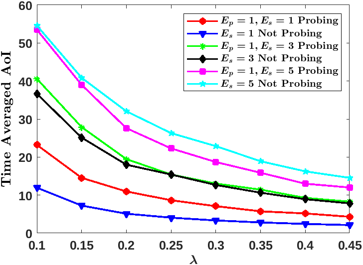
(a)

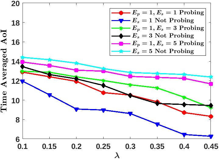
(b)

Figure 6: For $N=1$, Variation of time averaged AoI and comparison of a probing and non-probing system with change in $\lambda,E_{p}$ and $E_{s}$ for (a) I.I.D. model, (b) Markovian model.

VI-E Q-Learning

We consider the same settings as Section VI-A and Section VI-C, except that we set $B=5$ and an upper bound on the age as $T_{max}=7$, in order to reduce the number of possible states. We then run an online Q-learning scheme across two different sample paths. For the sake of comparison, we also plot the time averaged AoI of a uniform random strategy as well as that of the optimal policy derived through value iteration. Convergence of the time-averaged AoI under Q-learning to the optimal AoI for the i.i.d. channel system and the Markovian model can be seen in Figure 7 (a) and Figure 7 (b), respectively. We also observe significant improvement from the initial policy which always picks an action uniformly at random; this demonstrates the necessity of the MDP based formulation for probing and sampling.

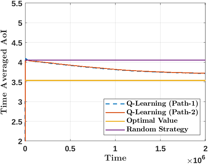
(a)

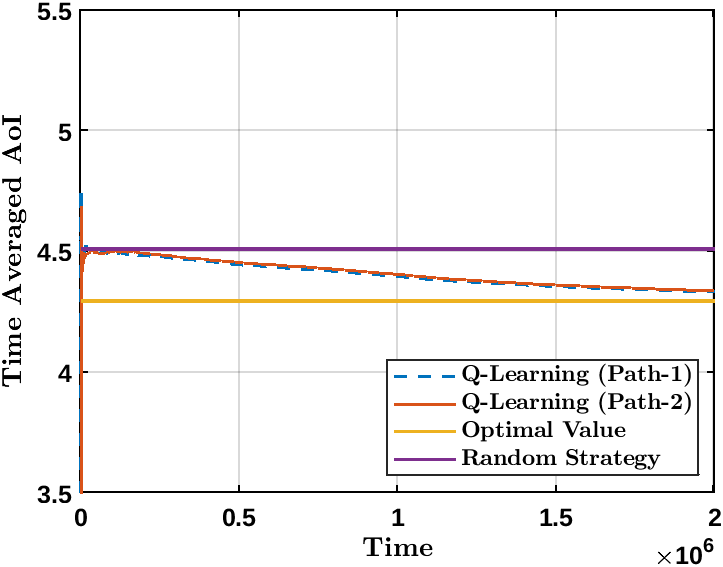
(b)

Figure 7: Improvement in time averaged AoI exhibited by Q-learning, $N=1$, (a) I.I.D. model, (b) Markovian model.

VII Conclusions

In this paper, we have derived optimal policy structures for minimizing the time-averaged expected AoI under an energy-harvesting source. We considered single and multiple processes, i.i.d. and Markovian time varying channels, time varying characteristics for energy harvesting, and channel probing capability at the source. The optimal source sampling policy often turned out to be a threshold policy. We have also proposed RL algorithms for unknown channel statistics and energy harvesting characteristics. However, there are a number of issues that remain untouched, such as multi-source star topology and multi-hop network setting with multiple source and sink nodes. We plan to address these issues in our future research endeavours.

Appendix A Proof of proposition 1

We prove that $max_{s\in\mathcal{S}}|J^{(t)}(s)-J^{*}(s)|\uparrow 0$ as $t\uparrow\infty$. Let us define the error $e_{t}=\max_{s\in\mathcal{S}}|J^{(t)}(s)-J^{*}(s)|$ and $J^{(0)}(s)$ as initial estimate for $J^{*}(s)$. For any state $s$, we seek to establish relation between the error at time $t+1$ to the error at time $t$.

$$J^{(t+1)}(E\geq E_{p}+E_{s},T)$$ (28)

$$= min\bigg{\{}T+\alpha\mathbb{E}_{A}J^{(t)}(min\{E+A,B\},T+1),$$

$$\mathbb{E}_{C}\bigg{(}min\{T+\alpha\mathbb{E}_{A}J^{(t)}(min\{E-E_{p}+A,B\},T+1),$$

$$T(1-p(C))+\alpha p(C)\mathbb{E}_{A}J^{(t)}(min\{E-E_{p}-E_{s}+A,B\},1)+$$

$$\alpha(1-p(C))\mathbb{E}_{A}J^{(t)}(min\{E-E_{p}-E_{s}+A,B\},T+1)\}\bigg{)}\bigg{\}}$$

We assume there exists an optimal value function $J^{*}(E,T)$ for the discounted cost problem. By using the fact that $J^{(t)}(E,T)\leq J^{*}(E,T)+e_{t}$ in (28), we obtain:

$$J^{(t+1)}(E\geq E_{p}+E_{s},T)$$ (29)

$$\leq min\bigg{\{}T+\alpha\mathbb{E}_{A}(J^{*}(min\{E+A,B\},T+1)+e_{t}),$$

$$\mathbb{E}_{C}\bigg{(}min\{T+\alpha\mathbb{E}_{A}(J^{*}(min\{E-E_{p}+A,B\},T+1)+e_{t}),$$

$$T(1-p(C))+\alpha p(C)\mathbb{E}_{A}(J^{*}(min\{E-E_{p}-E_{s}+A,B\},1)+e_{t})$$

$$+\alpha(1-p(C))\mathbb{E}_{A}(J^{*}(min\{E-E_{p}-E_{s}+A,B\},T+1)+e_{t})\}\bigg{)}\bigg{\}}$$

Similarly, using $J^{(t)}(E,T)\geq J^{*}(E,T)-e_{t}$ in (28), we obtain:

$$J^{(t+1)}(E\geq E_{p}+E_{s},T)$$ (30)

$$\geq min\bigg{\{}T+\alpha\mathbb{E}_{A}(J^{*}(min\{E+A,B\},T+1)-e_{t}),$$

$$\mathbb{E}_{C}\bigg{(}min\{T+\alpha\mathbb{E}_{A}(J^{*}(min\{E-E_{p}+A,B\},T+1)-e_{t}),$$

$$T(1-p(C))+\alpha p(C)\mathbb{E}_{A}(J^{*}(min\{E-E_{p}-E_{s}+A,B\},1)-e_{t})$$

$$+\alpha(1-p(C))\mathbb{E}_{A}(J^{*}(min\{E-E_{p}-E_{s}+A,B\},T+1)-e_{t})\}\bigg{)}\bigg{\}}$$

$$J^{*}(E\geq E_{p}+E_{s},T)-\alpha e_{t}$$ (31)

$$\leq J^{(t+1)}(E\geq E_{p}+E_{s},T)\leq J^{*}(E\geq E_{p}+E_{s},T)+\alpha e_{t}$$

$$\implies |J^{(t+1)}(E\geq E_{p}+E_{s},T)-J^{*}(E\geq E_{p}+E_{s},T)|\leq\alpha e_{t}$$

$$\implies \max_{s\in\mathcal{S}}|J^{(t+1)}(s)-J^{*}(s)|\leq\alpha e_{t}$$

$$\implies e_{t+1}\leq\alpha e_{t}$$

$$\implies \lim_{t\rightarrow\infty}e_{t}=0$$

Hence, $J^{(t)}(s)$ converges to $J^{*}(s)$.

Appendix B Proof of Lemma 1

We prove this result by value iteration:

$$J^{(t+1)}(E\geq E_{p}+E_{s},T)$$ (32)

$$= min\bigg{\{}T+\alpha\mathbb{E}_{A}J^{(t)}(min\{E+A,B\},T+1),$$

$$\mathbb{E}_{C}\bigg{(}min\{T+\alpha\mathbb{E}_{A}J^{(t)}(min\{E-E_{p}+A,B\},T+1),$$

$$T(1-p(C))+\alpha p(C)\mathbb{E}_{A}J^{(t)}(min\{E-E_{p}-E_{s}+A,B\},1)+$$

$$\alpha(1-p(C))\mathbb{E}_{A}J^{(t)}(min\{E-E_{p}-E_{s}+A,B\},T+1)\}\bigg{)}\bigg{\}}$$

$$J^{(t+1)}(E<E_{p}+E_{s},T)$$

$$= T+\alpha\mathbb{E}_{A}J^{(t)}(min\{E+A,B\},T+1)$$

Let us start with $J^{(0)}(s)=0$ for all $s\in S$. Clearly, $J^{(1)}(E\geq E_{p}+E_{s},T)=min\{T,\mathbb{E}_{C}(min\{T,T(1-p(C))\})\}$ $=min\{T,\mathbb{E}_{C}(T(1-p(C))\}$ and $J^{(1)}(E<E_{p}+E_{s},T)=T$. Hence, for any given $E$, the value function $J^{(1)}(E,T)$ is an increasing function of $T$. As induction hypothesis, we assume that $J^{(t)}(E,T)$ is also increasing function of $T$. Now,

$$J^{(t+1)}(E\geq E_{p}+E_{s},T)$$ (33)

$$= min\bigg{\{}T+\alpha\mathbb{E}_{A}J^{(t)}(min\{E+A,B\},T+1),$$

$$\mathbb{E}_{C}\bigg{(}min\{T+\alpha\mathbb{E}_{A}J^{(t)}(min\{E-E_{p}+A,B\},T+1),$$

$$T(1-p(C))+\alpha p(C)\mathbb{E}_{A}J^{(t)}(min\{E-E_{p}-E_{s}+A,B\},1)+$$

$$\alpha(1-p(C))\mathbb{E}_{A}J^{(t)}(min\{E-E_{p}-E_{s}+A,B\},T+1)\}\bigg{)}\bigg{\}}$$

We need to show that $J^{(t+1)}(E\geq E_{p}+E_{s},T)$ is also increasing in $T$. The first term inside the minimization operation in (33) is increasing in $T$, by the induction hypothesis and from the fact that expectation is a linear operation. On the other hand, the second term has linear expectation over channel state and another minimization operator. Also, the first and second terms inside the second minimization operation in (33) are increasing in $T$ by the induction hypothesis and the linearity of expectation operation. Thus, $J^{(t+1)}(E\geq E_{p}+E_{s},T)$ is also increasing in $T$. By similar arguments, we can claim that $J^{(t+1)}(E<E_{p}+E_{s},T)$ is increasing in $T$. Now, since $J^{(t)}(\cdot)\uparrow J^{*}(\cdot)$ as $t\uparrow\infty$ by proof of Proposition 1, $J^{*}(E,T)$ is also increasing in $T$. Hence, the first part of the lemma is proved.
For currrent probed channel state, the value function $W^{(t+1)}(E,T,C)$ is given by:

$$W^{(t+1)}(E,T,C)$$ (34)

$$= min\{T+\alpha\mathbb{E}_{A}J^{(t)}(min\{E-E_{p}+A,B\},T+1),$$

$$T(1-p(C))+\alpha p(C)\mathbb{E}_{A}J^{(t)}(min\{E-E_{p}-E_{s}+A,B\},1)+$$

$$\alpha(1-p(C))\mathbb{E}_{A}J^{(t)}(min\{E-E_{p}-E_{s}+A,B\},T+1)\}$$

The first term (cost of not sampling a source) inside the minimization operation in (34) is independent of $p(C)$, whereas the second term (cost of sampling a source) inside the minimization operation in (34) is given by:

$$T(1-p(C))+\alpha p(C)\mathbb{E}_{A}J^{(t)}(min\{E-E_{p}-E_{s}+A,B\},1)+$$ (35)

$$\alpha(1-p(C))\mathbb{E}_{A}J^{(t)}(min\{E-E_{p}-E_{s}+A,B\},T+1)$$

$$= T(1-p(C))+\alpha\mathbb{E}_{A}J^{(t)}(min\{E-E_{p}-E_{s}+A,B\},T+1)-$$

$$p(C)\alpha\bigg{(}\mathbb{E}_{A}J^{(t)}(min\{E-E_{p}-E_{s}+A,B\},T+1)-$$

$$\mathbb{E}_{A}J^{(t)}(min\{E-E_{p}-E_{s}+A,B\},1)\bigg{)}$$

By the induction hypothesis and the linearity of expectation operation, $\mathbb{E}_{A}J^{(t)}(min\{E-E_{p}-E_{s}+A,B\},T+1)-\mathbb{E}_{A}J^{(t)}(min\{E-E_{p}-E_{s}+A,B\},1)$ is non-negative. Thus, the second term inside the minimization operation in (34) is decreasing in $p(C)$. Now, since $W^{(t)}(\cdot)\uparrow W^{*}(\cdot)$ as $t\uparrow\infty$, $W^{*}(E,T,C)$ is also decreasing in $p(C)$.

Appendix C Proof of Theorem 1

From (3), it is obvious that for probed channel state the optimal decision for $E\geq E_{p}+E_{s}$ is to sample the source if and only if the cost of sampling is lower than the cost of not sampling the source, i.e., $T+\alpha\mathbb{E}_{A}J^{*}(min\{E-E_{p}+A,B\},T+1)\geq T(1-p(C))+\alpha\mathbb{E}_{A}J^{*}(min\{E-E_{p}-E_{s}+A,B\},T+1)-\alpha p(C)\bigg{(}\mathbb{E}_{A}J^{*}(min\{E-E_{p}-E_{s}+A,B\},T+1)-\mathbb{E}_{A}J^{*}(min\{E-E_{p}-E_{s}+A,B\},1)\bigg{)}$. Now, by Lemma 1, $\mathbb{E}_{A}J^{*}(min\{E-E_{p}-E_{s}+A,B\},T+1)-\mathbb{E}_{A}J^{*}(min\{E-E_{p}-E_{s}+A,B\},1)$ is non-negative. Thus the R.H.S. decreases with $p(C)$, whereas the L.H.S. is independent of $p(C)$. Hence, for probed channel state the optimal action is to sample if and only if $p(C)\geq p_{th}(E,T)$ for some suitable threshold function $p_{th}(E,T)$.

Appendix D Proof of Lemma 2

The proof is similar to the proof of Lemma 1 and it follows from the convergence of value iteration as given below:

$$J^{(t+1)}(E\geq E_{p}+E_{s},T_{1},T_{2},\cdots,T_{N})$$

$$= min\bigg{\{}\sum_{i=1}^{N}T_{i}+\alpha\mathbb{E}_{A}J^{(t)}(min\{E+A,B\},T_{1}+1,T_{2}+1,\cdots,T_{N}+1),$$

$$\mathbb{E}_{C}\bigg{(}min\{\sum_{i=1}^{N}T_{i}+\alpha\mathbb{E}_{A}J^{(t)}(min\{E-E_{p}+A,B\},T_{1}+1,T_{2}+1,\cdots,$$

$$T_{N}+1),\min_{1\leq k\leq N}\bigg{(}\sum_{i\neq k}T_{i}+T_{k}(1-p(C))+\alpha p(C)\mathbb{E}_{A}J^{(t)}(min\{E-E_{p}$$

$$-E_{s}+A,B\},T_{1}+1,T_{2}+1,\cdots,T_{k}^{\prime}=1,T_{k+1}+1,\cdots,T_{N}+1)+$$

$$\alpha(1-p(C))\mathbb{E}_{A}J^{(t)}(min\{E-E_{p}-E_{s}+A,B\},T_{1}+1,T_{2}+1,\cdots,$$

$$T_{N}+1)\bigg{)}\}\bigg{)}\bigg{\}}$$

$$J^{(t+1)}(E<E_{p}+E_{s},T_{1},T_{2},\cdots,T_{N})$$

$$= \sum_{i=1}^{N}T_{i}+\alpha\mathbb{E}_{A}J^{(t)}(min\{E+A,B\},T_{1}+1,T_{2}+1,\cdots,T_{N}+1)$$

Let us start with $J^{(0)}(s)=0$ for all $s\in S$. Clearly, $J^{(1)}(E\geq E_{p}+E_{s},T_{1},T_{2},\cdots,T_{N})=\min\{\sum_{i=1}^{N}T_{i},\mathbb{E}_{C}(min\{\sum_{i=1}^{N}T_{i},\min_{1\leq k\leq N}(\sum_{i\neq k}T_{i}+T_{k}(1-p(C)))\}\}$ and $J^{(1)}(E<E_{p}+E_{s},T_{1},T_{2},\cdots,T_{N})=\sum_{i=1}^{N}T_{i}$. Hence, for any given $E$, the value function $J^{(1)}(E,T_{1},T_{2},\cdots,T_{N})$ is an increasing function of $T_{1},T_{2},\cdots,T_{N}$. As induction hypothesis, we assume that $J^{(t)}(E,T_{1},T_{2},\cdots,T_{N})$ is also increasing function of $T_{1},T_{2},\cdots,T_{N}$. Now,

$$J^{(t+1)}(E\geq E_{p}+E_{s},T_{1},T_{2},\cdots,T_{N})$$ (37)

$$= min\bigg{\{}\sum_{i=1}^{N}T_{i}+\alpha\mathbb{E}_{A}J^{(t)}(min\{E+A,B\},T_{1}+1,T_{2}+1,\cdots,T_{N}+1),$$

$$\mathbb{E}_{C}\bigg{(}min\{\sum_{i=1}^{N}T_{i}+\alpha\mathbb{E}_{A}J^{(t)}(min\{E-E_{p}+A,B\},T_{1}+1,T_{2}+1,\cdots,$$

$$T_{N}+1),\min_{1\leq k\leq N}\bigg{(}\sum_{i\neq k}T_{i}+T_{k}(1-p(C))+\alpha p(C)\mathbb{E}_{A}J^{(t)}(min\{E-E_{p}$$

$$-E_{s}+A,B\},T_{1}+1,T_{2}+1,\cdots,T_{k}^{\prime}=1,T_{k+1}+1,\cdots,T_{N}+1)+$$

$$\alpha(1-p(C))\mathbb{E}_{A}J^{(t)}(min\{E-E_{p}-E_{s}+A,B\},T_{1}+1,T_{2}+1,\cdots,$$

$$T_{N}+1)\bigg{)}\}\bigg{)}\bigg{\}}$$

We seek to show that $J^{(t+1)}(E\geq E_{p}+E_{s},T_{1},T_{2},\cdots,T_{N})$ is also increasing in each of $T_{1},T_{2},\cdots,T_{N}$. The first term inner to the minimization operation in (37) is increasing in each of $T_{1},T_{2},\cdots,T_{N}$, utilizing the induction hypothesis and linear property of expectation operation. On the other hand, the second term has expectation over channel state and another minimization operator. Also, the fist and second term of second minimization operator is increasing in each of $T_{1},T_{2},\cdots,T_{N}$ by using induction hypothesis and the linearity of expectation operation. Thus, $J^{(t+1)}(E\geq E_{p}+E_{s},T_{1},T_{2},\cdots,T_{N})$ is also increasing in each of $T_{1},T_{2},\cdots,T_{N}$. Similarly, we can assert that $J^{(t+1)}(E<E_{p}+E_{s},T_{1},T_{2},\cdots,T_{N})$ is increasing in each of $T_{1},T_{2},\cdots,T_{N}$. Now, since $J^{(t)}(\cdot)\uparrow J^{*}(\cdot)$ as $t\uparrow\infty$, $J^{*}(E,T_{1},T_{2},\cdots,T_{N})$ is also increasing in each of $T_{1},T_{2},\cdots,T_{N}$. Hence, the first part of the lemma is proved. Proof of second part of Lemma 2 is similar to the proof of second part of Lemma 1

Appendix E Proof of Theorem  2

It is obvious that $J^{*}(\cdot)$ is invariant to any permutation of $(T_{1},T_{2},\cdots,T_{N})$. Hence, by Lemma 2, $\arg\min_{1\leq k\leq N}\bigg{(}\sum_{i\neq k}T_{i}+T_{k}(1-p(C))+\alpha p(C)\mathbb{E}_{A}J^{(t)}(min\{E-E_{p}-E_{s}+A,B\},T_{1}+1,T_{2}+1,\cdots,T_{k}^{\prime}=1,T_{k+1}+1,\cdots,T_{N}+1)+\alpha(1-p(C))\mathbb{E}_{A}J^{(t)}(min\{E-E_{p}-E_{s}+A,B\},T_{1}+1,T_{2}+1,\cdots,T_{N}+1)\bigg{)}=\arg\max_{1\leq k\leq N}T_{k}$, i.e., the best process to activate is $k^{*}\doteq\arg\max_{1\leq k\leq N}T_{k}$ in case one process has to be activated. For probed channel state, it is optimal to sample a process if and only if the cost of sampling this process is less than or equal to the cost of not sampling this process, which translates into $T_{k^{*}}+\alpha\mathbb{E}_{A}J^{*}(min\{E-E_{p}+A,B\},T_{1}+1,T_{2}+1,\cdots,T_{N}+1)\geq T_{k^{*}}(1-p(C))+\alpha\mathbb{E}_{A}J^{*}(min\{E-E_{p}-E_{s}+A,B\},T_{1}+1,T_{2}+1,\cdots,T_{N}+1)-\alpha p(C)\bigg{(}\mathbb{E}_{A}J^{*}(min\{E-E_{p}-E_{s}+A,B\},T_{1}+1,T_{2}+1,\cdots,T_{N}+1)-\mathbb{E}_{A}J^{*}(min\{E-E_{p}-E_{s}+A,B\},T_{1}+1,T_{2}+1,\cdots,T_{k}^{\prime}=1,T_{k+1}+1,\cdots,T_{N}+1)\bigg{)}$. Now, by Lemma 2, $\mathbb{E}_{A}J^{*}(min\{E-E_{p}-E_{s}+A,B\},T_{1}+1,T_{2}+1,\cdots,T_{N}+1)-\mathbb{E}_{A}J^{*}(min\{E-E_{p}-E_{s}+A,B\},T_{1}+1,T_{2}+1,\cdots,T_{k}^{\prime}=1,T_{k+1}+1,\cdots,T_{N}+1)$ is non negative. Thus, the R.H.S. is decreasing in $p(C)$ and the L.H.S. is independent of $p(C)$. Hence, the threshold structure of the optimal sampling policy is proved.

References

- [1] A. Jaiswal and A. Chattopadhyay, “Minimization of age-of-information in remote sensing with energy harvesting,” in 2021 IEEE International Symposium on Information Theory (ISIT). IEEE, 2021, pp. 3249–3254.
- [2] S. Kaul, R. Yates, and M. Gruteser, “Real-time status: How often should one update?” in 2012 Proceedings IEEE INFOCOM. IEEE, 2012, pp. 2731–2735.
- [3] R. Talak, S. Karaman, and E. Modiano, “Can determinacy minimize age of information?” arXiv preprint arXiv:1810.04371, 2018.
- [4] S. K. Kaul, R. D. Yates, and M. Gruteser, “Status updates through queues,” in 2012 46th Annual Conference on Information Sciences and Systems (CISS). IEEE, 2012, pp. 1–6.
- [5] R. D. Yates and S. K. Kaul, “The age of information: Real-time status updating by multiple sources,” IEEE Transactions on Information Theory, vol. 65, no. 3, pp. 1807–1827, 2018.
- [6] S. K. Kaul and R. D. Yates, “Timely updates by multiple sources: The m/m/1 queue revisited,” in 2020 54th Annual Conference on Information Sciences and Systems (CISS). IEEE, 2020, pp. 1–6.
- [7] A. Kosta, N. Pappas, A. Ephremides, and V. Angelakis, “Age of information performance of multiaccess strategies with packet management,” Journal of Communications and Networks, vol. 21, no. 3, pp. 244–255, 2019.
- [8] S. Farazi, A. G. Klein, and D. R. Brown, “Age of information in energy harvesting status update systems: When to preempt in service?” in 2018 IEEE International Symposium on Information Theory (ISIT). IEEE, 2018, pp. 2436–2440.
- [9] A. Arafa and S. Ulukus, “Age-minimal transmission in energy harvesting two-hop networks,” in GLOBECOM 2017-2017 IEEE Global Communications Conference. IEEE, 2017, pp. 1–6.
- [10] S. Farazi, A. G. Klein, and D. R. Brown, “Average age of information for status update systems with an energy harvesting server,” in IEEE INFOCOM 2018-IEEE Conference on Computer Communications Workshops (INFOCOM WKSHPS). IEEE, 2018, pp. 112–117.
- [11] H. Hu, K. Xiong, Y. Zhang, P. Fan, T. Liu, and S. Kang, “Age of information in wireless powered networks in low snr region for future 5g,” Entropy, vol. 20, no. 12, p. 948, 2018.
- [12] A. Arafa and S. Ulukus, “Age minimization in energy harvesting communications: Energy-controlled delays,” in 2017 51st Asilomar Conference on Signals, Systems, and Computers. IEEE, 2017, pp. 1801–1805.
- [13] Z. Chen, N. Pappas, E. Björnson, and E. G. Larsson, “Age of information in a multiple access channel with heterogeneous traffic and an energy harvesting node,” in IEEE INFOCOM 2019-IEEE Conference on Computer Communications Workshops (INFOCOM WKSHPS). IEEE, 2019, pp. 662–667.
- [14] X. Wu, J. Yang, and J. Wu, “Optimal status update for age of information minimization with an energy harvesting source,” IEEE Transactions on Green Communications and Networking, vol. 2, no. 1, pp. 193–204, 2017.
- [15] J. Yang, X. Wu, and J. Wu, “Optimal scheduling of collaborative sensing in energy harvesting sensor networks,” IEEE Journal on Selected Areas in Communications, vol. 33, no. 3, pp. 512–523, 2015.
- [16] B. T. Bacinoglu, Y. Sun, E. Uysal-Bivikoglu, and V. Mutlu, “Achieving the age-energy tradeoff with a finite-battery energy harvesting source,” in 2018 IEEE International Symposium on Information Theory (ISIT). IEEE, 2018, pp. 876–880.
- [17] S. Feng and J. Yang, “Age of information minimization for an energy harvesting source with updating erasures: With and without feedback,” arXiv preprint arXiv:1808.05141, 2018.
- [18] B. T. Bacinoglu, E. T. Ceran, and E. Uysal-Biyikoglu, “Age of information under energy replenishment constraints,” in 2015 Information Theory and Applications Workshop (ITA). IEEE, 2015, pp. 25–31.
- [19] S. Leng and A. Yener, “Age of information minimization for an energy harvesting cognitive radio,” IEEE Transactions on Cognitive Communications and Networking, vol. 5, no. 2, pp. 427–439, 2019.
- [20] E. Gindullina, L. Badia, and D. Gündüz, “Age-of-information with information source diversity in an energy harvesting system,” arXiv preprint arXiv:2004.11135, 2020.
- [21] E. T. Ceran, D. Gündüz, and A. György, “Reinforcement learning to minimize age of information with an energy harvesting sensor with harq and sensing cost,” in IEEE INFOCOM 2019-IEEE Conference on Computer Communications Workshops (INFOCOM WKSHPS). IEEE, 2019, pp. 656–661.
- [22] A. Arafa, J. Yang, and S. Ulukus, “Age-minimal online policies for energy harvesting sensors with random battery recharges,” in 2018 IEEE International Conference on Communications (ICC). IEEE, 2018, pp. 1–6.
- [23] C. Tunc and S. Panwar, “Optimal transmission policies for energy harvesting age of information systems with battery recovery,” in 2019 53rd Asilomar Conference on Signals, Systems, and Computers. IEEE, 2019, pp. 2012–2016.
- [24] B. T. Bacinoglu and E. Uysal-Biyikoglu, “Scheduling status updates to minimize age of information with an energy harvesting sensor,” in 2017 IEEE International Symposium on Information Theory (ISIT). IEEE, 2017, pp. 1122–1126.
- [25] M. A. Abd-Elmagid, H. S. Dhillon, and N. Pappas, “A reinforcement learning framework for optimizing age of information in rf-powered communication systems,” IEEE Transactions on Communications, vol. 68, no. 8, pp. 4747–4760, 2020.
- [26] M. Hatami, M. Leinonen, and M. Codreanu, “Aoi minimization in status update control with energy harvesting sensors,” arXiv preprint arXiv:2009.04224, 2020.
- [27] A. Arafa, J. Yang, S. Ulukus, and H. V. Poor, “Timely status updating over erasure channels using an energy harvesting sensor: Single and multiple sources,” IEEE Transactions on Green Communications and Networking, 2021.
- [28] G. Yao, A. M. Bedewy, and N. B. Shroff, “Age-optimal low-power status update over time-correlated fading channel,” in 2021 IEEE International Symposium on Information Theory (ISIT). IEEE, 2021, pp. 2972–2977.
- [29] N. Michelusi, K. Stamatiou, and M. Zorzi, “Transmission policies for energy harvesting sensors with time-correlated energy supply,” IEEE Transactions on Communications, vol. 61, no. 7, pp. 2988–3001, 2013.
- [30] B. Sombabu and S. Moharir, “Age-of-information aware scheduling under markovian energy arrivals,” in 2020 International Conference on Signal Processing and Communications (SPCOM). IEEE, 2020, pp. 1–5.
- [31] D. P. Bertsekas, “Dynamic programming and optimal control 3rd edition, volume ii,” Belmont, MA: Athena Scientific, 2011.
- [32] S. Bhatnagar, H. Prasad, and L. Prashanth, Stochastic Recursive Algorithms for Optimization: Simultaneous Perturbation Methods. Springer, 2013.
- [33] V. S. Borkar, “Asynchronous stochastic approximations,” SIAM Journal on Control and Optimization, vol. 36, no. 3, pp. 840–851, 1998.
- [34] S. Bhatnagar, “The borkar–meyn theorem for asynchronous stochastic approximations,” Systems & control letters, vol. 60, no. 7, pp. 472–478, 2011.