Non-classicality criteria for N-dimensional optical fields detected by quadratic detectors

Abstract

Non-classicality criteria for general $N$-dimensional optical fields are derived. They involve intensity moments, the probabilities of photon-number distributions or combinations of both. The Hillery criteria for the sums of the probabilities of even or odd photon numbers are generalized to $N$-dimensional fields. As an example, the derived non-classicality criteria are applied to an experimental 3-mode optical field containing two types of photon-pair contributions. The accompanying non-classicality depths are used to mutually compare their performance.

I Introduction

Identification of non-classicality of optical fields Mandel and Wolf (1995) has a long-lasting tradition in quantum optics. For many years, the non-classicality was identified and quantified by specific physical quantities suitable for revealing the non-classicality of different kinds of quantum fields Mandel and Wolf (1995). The Fano factor that quantifies the strength of photon-number fluctuations and the principal squeeze variance Lukš et al. (1988) that measures the squeezing of field phase fluctuations serve as typical examples. With the fast development of quantum optics, a large variety of nonclassical fields has been suggested and experimentally realized Dodonov (2002); Lvovsky and Raymer (2009). Many of them have no distinct properties that would allow to tailor specific non-classicality criteria (NCCa) for them. For this reason, the NCCa started to be investigated from the general point of view.

Here, we address the NCCa based on the measurement of photon-number distributions Peřina (1991) by quadratic detectors. Though these criteria are not sensitive to the phases of optical fields, they are extraordinarily useful for (spatio-spectrally) multi-mode optical fields. The multi-mode character of these fields implies that their statistical properties are fully characterized by photon-number measurements. The NCCa are traditionally written as the non-classicality inequalities that involve the moments of integrated intensities. These integrated-intensity moments denote the normally-ordered photon number moments Peřina (1991) that are derived from the photon-number distributions and their usual photon-number moments with the help of the commutation relations Peřina Jr. et al. (2020a). A great deal of attention has been devoted to such NCCa for 1-dimensional (1D) Short and Mandel (1983); Teich and Saleh (1985); Lee (1990a) and 2-dimensional (2D) Allevi et al. (2012, 2013); Sperling et al. (2015); Harder et al. (2016); Magańa-Loaiza et al. (2019); Peřina Jr. et al. (2021a, b) optical fields for practical reasons. Among others, they allow to identify the non-classicality of sub-Poissonian fields (1D) and twin beams (2D). Useful NCCa were derived by several approaches including the Cauchy-Schwarz inequality, majorization theory and by using the classically nonnegative polynomials. They were summarized in Ref. Arkhipov et al. (2016) for 1D and in Ref. Peřina Jr. et al. (2017a) for 2D optical fields.

Klyshko suggested in Ref. Klyshko (1996) the use of the Mandel detection formula Mandel and Wolf (1995); Peřina (1991) in combination with the NCCa involving the intensity moments to arrive at the NCCa written in the photon-number probabilities. These criteria are in general more sensitive to the non-classicality Waks et al. (2004, 2006); Wakui et al. (2014); Peřina Jr. et al. (2017b). Some of them also allow to identify the regions of photon-number distributions where the non-classicality resides. They were extensively studied in Ref. Peřina Jr. et al. (2020b) for 1D and Ref. Peřina Jr. et al. (2020a) for 2D optical fields.

The 1D and 2D NCCa represent special variants of the general NCCa written for arbitrary dimensions and addressed in this paper. They are applied to marginal 1D and 2D fields of the general $N$-dimensional fields obtained by tracing out over the remaining dimensions. Thus the NCCa for dimensions greater than two are in principle more general than those written in 1D and 2D. They are indispensable for identification and quantification of the non-classicality of fields exhibiting genuine higher-order quantum correlations. This is topical for 3-dimensional (3D) fields generated in the process of third-harmonic generation (triples of photons) Chekhova et al. (2005), cascaded second-order processes Shalm et al. (2013); Hamel et al. (2014) or by post-selection Alexander et al. (2020) (GHZ-like states).

Here, we provide the derivation of the NCCa for general $N$-dimensional optical fields by generalizing the approaches applied earlier to 1D and 2D optical fields. We reveal general relations among the derived NCCa. We show that the commonly used NCCa originating in the matrix approach using $2\times 2$ matrices form a subset inside the group of the NCCa stemming from the Cauchy-Schwarz inequality. We further show that the NCCa provided by the majorization theory can be decomposed into the much simpler ones. These fundamental NCCa can easily be derived assuming simple non-negative polynomials. In general, we identify the fundamental non-classicality inequalities, i.e. the inequalities that are not implied by other even simpler non-classicality inequalities. We develop the approach for deriving an $N$-dimensional form of the Hillery non-classicality criteria Hillery (1985). We also suggest a new type of the NCCa - the hybrid NCCa. They contain the field intensity moments in some dimensions while using the probabilities of photon-number distributions in the remaining dimensions.

The NCCa allow not only to identify the non-classicality. They are useful in quantifying the non-classicality when the Lee concept of non-classicality depth (NCD) Lee (1991) or non-classicality counting parameter Peřina Jr. et al. (2019) are applied. This allows to judge the performance of NCCa and identify the NCCa suitable for revealing the non-classicality for given types of nonclassical states. Moreover, when greater number of the NCCa is applied, the maximal reached NCDs are assumed to give fair estimate of the overall non-classicality of the analyzed state. This is important in numerous applications that exploit nonclassical states.

We note that the NCCa can also be applied to optical fields that are modified before detection. This improves the ability of the NCCa to reveal the non-classicality. Mixing of an analyzed field with a known coherent state at a beam-splitter serves as a typical example Kuhn et al. (2017); Arkhipov (2018).

To demonstrate the performance of the derived NCCa, we apply the derived NCCa to a 3D optical field that is built from two photon-pair contributions. This example allows us to demonstrate the main features of the derived NCCa.

The paper is organized as follows. We bring the intensity NCCa in Sec. II whose subsections are devoted to specific kinds of the NCCa. The probability NCCa are summarized in Sec. III. Hybrid criteria are introduced in Sec. IV. The general derivation of the Hillery criteria is contained in Sec. V. Section VI is devoted to non-classicality quantification. As an example, an experimental 3D optical field with pairwise correlations is analyzed in Sec. VII. Conclusions are drawn in Sec. VIII.

II Intensity non-classicality criteria

In this section, we pay attention to the non-classicality inequalities that use the (integrated) intensity moments Peřina (1991). In the following subsections, we apply the Cauchy-Schwarz inequality, the matrix approach, the majorization theory and the method that uses nonnegative polynomials to arrive at the intensity NCCa in $N$ dimensions. We consider $N$ fields described by their intensities $W_{j}$ and photon numbers $n_{j}$, $j=1,\ldots,N$. To formally simplify the description we write the intensities $W_{j}$ of the constituting fields as the elements of an $N$-dimensional intensity vector ${\bf W}\equiv\{W_{1},\ldots,W_{N}\}$. Similarly the corresponding photon numbers $n_{j}$ occurring in the detection of the constituting fields are conveniently arranged into a photon-number vector ${\bf n}\equiv\{n_{1},\ldots,n_{N}\}$. The joint state of these fields is characterized by the joint quasi-distribution $P({\bf W})$ of integrated intensities and joint photon-number distribution $p({\bf n})$. Intensity moments of the overall field can then be expressed as $\langle{\bf W}^{\bf i}\rangle\equiv\langle W_{1}^{i_{1}}\cdots W_{N}^{i_{N}}\rangle$ using the integer vector ${\bf i}\equiv\{i_{1},\ldots,i_{N}\}$ containing the powers in individual dimensions. We also introduce the notation for $N$-dimensional factorial ${\bf i}!\equiv i_{1}!\ldots i_{N}!$.

II.1 Intensity criteria based on the Cauchy-Schwarz inequality

For 2D optical fields, the Cauchy-Schwarz inequality provides a group of powerful criteria Peřina Jr. et al. (2017b, 2020a). When we consider the real functions $f({\bf W})={\bf W}^{{\bf l}/2+{\bf k}}$ and $g({\bf W})={\bf W}^{{\bf l}/2+{\bf k}^{\prime}}$ for arbitrary integer vectors ${\bf l}$, ${\bf k}$ and ${\bf k}^{\prime}$, the Cauchy-Schwarz inequality $|\int f({\bf W})g({\bf W})P({\bf W})d{\bf W}|^{2}\leq\int f^{2}({\bf W})P({\bf W})d{\bf W}\int g^{2}({\bf W})P({\bf W})d{\bf W}$ written for a classical nonnegative probability distribution $P({\bf W})$ takes the form:

$$\langle{\bf W}^{{\bf l}+{\bf k}+{\bf k}^{\prime}}\rangle^{2}\leq\langle{\bf W}^{{\bf l}+2{\bf k}}\rangle\langle{\bf W}^{{\bf l}+2{\bf k}^{\prime}}\rangle,$$ (1)

where we use the notation $\langle\ldots\rangle=\int d{\bf W}P({\bf W})\ldots$ for the mean value and $d{\bf W}\equiv dW_{1}\cdots dW_{N}$. Introducing the integer vectors ${\bf n}={\bf l}+{\bf k}+{\bf k}^{\prime}$ and ${\bf m}={\bf l}+2{\bf k}$ we derive the following NCCa from the classical inequality (1):

$$C_{\bf n}^{\bf m}=\langle{\bf W}^{\bf m}\rangle\langle{\bf W}^{2{\bf n}-{\bf m}}\rangle-\langle{\bf W}^{\bf n}\rangle^{2}<0.$$ (2)

II.2 Intensity criteria based on the matrix approach

Nonnegative quadratic forms are conveniently written in the matrix form. Their consideration leads to powerful and versatile NCCa for 1D Arkhipov et al. (2016) and 2D Agarwal and Tara (1992); Shchukin et al. (2005); Vogel (2008); Miranowicz et al. (2010) optical fields. Considering determinant of the $2\times 2$ matrix

$${\rm det}\langle\left[\begin{array}[]{cc}{\bf W}^{2{\bf k}}&{\bf W}^{{\bf k}+{\bf l}}\\ {\bf W}^{{\bf l}+{\bf k}}&{\bf W}^{2{\bf l}}\end{array}\right]\rangle=\langle{\bf W}^{2{\bf k}}\rangle\langle{\bf W}^{2{\bf l}}\rangle-\langle{\bf W}^{{\bf k}+{\bf l}}\rangle^{2}$$ (5)

describing the quadratic form $({\bf W}^{\bf k}+{\bf W}^{\bf l})^{2}$ we arrive at the NCCa that form a subset of the group $C_{\bf n}^{\bf m}$ in Eq. (2) [${\bf n}\leftarrow{\bf k}+{\bf l}$, ${\bf m}\leftarrow 2{\bf l}$].

On the other hand, the quadratic form $({\bf W}^{\bf k}+{\bf W}^{\bf l}+{\bf W}^{\bf m})^{2}$ encoded into the $3\times 3$ matrix

$$\left[\begin{array}[]{ccc}{\bf W}^{2{\bf k}}&{\bf W}^{{\bf k}+{\bf l}}&{\bf W}^{{\bf k}+{\bf m}}\\ {\bf W}^{{\bf l}+{\bf k}}&{\bf W}^{2{\bf l}}&{\bf W}^{{\bf l}+{\bf m}}\\ {\bf W}^{{\bf m}+{\bf k}}&{\bf W}^{{\bf m}+{\bf l}}&{\bf W}^{2{\bf m}}\end{array}\right]$$ (9)

provides the powerful NCCa with the complex structure:

$$M_{\bf klm}=\bigl{\{}\langle{\bf W}^{2{\bf k}}\rangle[\langle{\bf W}^{2{\bf l}}\rangle\langle{\bf W}^{2{\bf m}}\rangle-\langle{\bf W}^{{\bf l}+{\bf m}}\rangle^{2}]$$

$$+({\bf klm})\leftarrow({\bf lmk})+({\bf klm})\leftarrow({\bf mkl})\bigr{\}}$$

$$+2[\langle{\bf W}^{{\bf k}+{\bf l}}\rangle\langle{\bf W}^{{\bf k}+{\bf m}}\rangle\langle{\bf W}^{{\bf l}+{\bf m}}\rangle-\langle{\bf W}^{2{\bf k}}\rangle\langle{\bf W}^{2{\bf l}}\rangle\langle{\bf W}^{2{\bf m}}\rangle]$$

$$<0.$$ (10)

Symbol $\leftarrow$ used in Eq. (10) stands for the terms derived from the explicitly written ones by the indicated change of indices.

II.3 Intensity criteria originating in majorization theory and nonnegative polynomials

In the majorization theory Marshall et al. (2010) many classical inequalities for polynomials written in fixed numbers of independent variables are derived Lee (1990b). The inequalities describing ’the movement of one ball towards the right’ Marshall et al. (2010) represent the basic building blocks of the remaining inequalities. Assuming the integer vectors ${\bf i}$ and ${\bf i}^{\prime}=\{i_{1},\ldots,i_{k}+1,\ldots,i_{l}-1,\ldots,i_{N}\}$, $k<l$, such that the vector ${\bf i}^{\prime}$ majorizes the vector ${\bf i}$ (${\bf i}^{\prime}\succ{\bf i}$, $i_{1}-1\geq i_{2}-1\geq\ldots\geq i_{k-1}-1\geq i_{k}\geq\ldots\geq i_{l}\geq i_{l+1}+1\geq\ldots\geq i_{N}+1$) they give rise to the following non-classicality inequalities:

$$\sum_{{\cal P}{\bf i}^{\prime}}\langle{\bf W}^{{\bf i}^{\prime}}\rangle<\sum_{{\cal P}{\bf i}}\langle{\bf W}^{{\bf i}}\rangle.$$ (11)

In Eq. (11), symbol $\cal P{\bf i}$ stands for all permutations of the elements of vector $\bf i$.

The non-classicality inequalities (11) can be conveniently decomposed into the much simpler ones expressed as:

$$E_{\bf i}^{kl}=\langle{\bf W}^{\bf i}(W_{k}-W_{l})^{2}\rangle=\langle{\bf W}_{kl}^{{\bf i}_{kl}^{\perp}}(W_{k}^{i_{k}+2}W_{l}^{i_{l}}$$

$$-2W_{k}^{i_{k}+1}W_{l}^{i_{l}+1}+W_{k}^{i_{k}}W_{l}^{i_{l}+2})\rangle<0;$$ (12)

${\bf W}_{kl}=W_{1}\ldots W_{k-1}W_{k+1}\ldots W_{l-1}W_{l+1}\ldots W_{N}$ and ${\bf i}_{kl}^{\perp}=\{i_{1},\ldots,i_{k-1},i_{k+1},\ldots,i_{l-1},i_{l+1},\ldots,i_{N}\}$. The inequality (11) can be expressed in terms of the simpler inequalities $E_{\bf i}^{kl}$ as follows ($i_{k}\geq i_{l}$):

$$\sum_{k^{\prime}=1}^{N}\sum_{l^{\prime}=1}^{k^{\prime}-1}\sum_{{\cal P}{\bf i}_{k^{\prime}l^{\prime}}^{\perp}}\Bigl{[}E_{{\cal P}_{k}^{k^{\prime}}{\cal P}_{l}^{l^{\prime}}\{\ldots,i_{k}-1,\ldots,i_{l}-1,\ldots\}}^{k^{\prime}l^{\prime}}$$

$$+E_{{\cal P}_{k}^{k^{\prime}}{\cal P}_{l}^{l^{\prime}}\{\ldots,i_{k}-2,\ldots,i_{l},\ldots\}}^{k^{\prime}l^{\prime}}+E_{{\cal P}_{k}^{k^{\prime}}{\cal P}_{l}^{l^{\prime}}\{\ldots,i_{k}-3,\ldots,i_{l}+1,\ldots\}}^{k^{\prime}l^{\prime}}$$

$$+\ldots+E_{{\cal P}_{k}^{k^{\prime}}{\cal P}_{l}^{l^{\prime}}\{\ldots,i_{l}+1,\ldots,i_{k}-3,\ldots\}}^{k^{\prime}l^{\prime}}+E_{{\cal P}_{k}^{k^{\prime}}{\cal P}_{l}^{l^{\prime}}\{\ldots,i_{l},\ldots,i_{k}-2,\ldots\}}^{k^{\prime}l^{\prime}}$$

$$+E_{{\cal P}_{k}^{k^{\prime}}{\cal P}_{l}^{l^{\prime}}\{\ldots,i_{l}-1,\ldots,i_{k}-1,\ldots\}}^{k^{\prime}l^{\prime}}\Bigr{]}<0$$ (13)

and ${\cal P}_{k}^{k^{\prime}}\{\ldots,i_{k},\ldots,i_{k^{\prime}},\ldots\}=\{\ldots,i_{k^{\prime}},\ldots,i_{k},\ldots\}$.

As a consequence, any non-classicality inequality stemming from the majorization theory is implied by the non-classicality inequalities $E_{\bf i}^{kl}$ given in Eq. (12). They can simply be generalized into the NCCa

$$E_{\bf i}^{\bf I}=\langle{\bf W}^{\bf i}\prod_{k=1}^{N}\prod_{l=k+1}^{N}(W_{k}-W_{l})^{2I_{kl}}\rangle<0$$ (14)

in which the integers $I_{kl}$ form an upper triangular matrix ${\bf I}$.

Also other NCCa based on nonnegative polynomials can be constructed. They are useful for the states with specific forms of correlations. As an example we write the NCCa $P^{k}$ and $P^{kl}$,

$$P^{k} = \langle\left(\sum_{k^{\prime}=1}^{N}W_{k^{\prime}}-2W_{k}\right)^{2}\rangle,$$ (15)

$$P^{kl} = \langle\left(\sum_{k^{\prime}=1}^{N}W_{k^{\prime}}-2W_{k}\right)^{2}\left(\sum_{l^{\prime}=1}^{N}W_{l^{\prime}}-2W_{l}\right)^{2}\rangle,$$ (16)

useful for the non-classicality analysis of the states in Sec. VI.

III Probability non-classicality criteria

The Mandel detection formula Mandel and Wolf (1995); Peřina (1991) written for an $N$-dimensional optical field as

$$p({\bf n})=\frac{1}{{\bf n}!}\int d{\bf W}{\bf W}^{\bf n}\exp(-\Sigma{\bf W})P({\bf W}),$$ (17)

$\Sigma{\bf W}=\sum_{k=1}^{N}W_{k}$, allows to derive the probability NCCa from the corresponding intensity NCCa according to the following mapping (for details, see the next section):

$${\bf W}^{\bf n}\leftarrow{\bf n}!p({\bf n})/p({\bf 0});$$ (18)

symbol ${\bf 0}$ denotes the vector with all elements equal to 0.

Using the mapping (18), the intensity NCCa $C_{\bf n}^{\bf m}$ from Eq. (5) derived from the Cauchy-Schwarz inequality give the following probability NCCa:

$$\bar{C}_{\bf n}^{\bf m}=\frac{(2\bf{n}-{\bf m})!{\bf m}!}{({\bf n}!)^{2}}p({\bf m})p(2{\bf n}-{\bf m})-p^{2}({\bf n})<0.$$ (19)

Similarly, the intensity NCCa $M_{\bf klm}$ in Eq. (10) obtained by the matrix approach are transformed into the following probability NCCa:

$$\bar{M}_{\bf klm}=\Bigl{\{}p(2{\bf k})\Bigl{[}p(2{\bf l})p(2{\bf m})-\frac{({\bf l}+{\bf m})!^{2}}{(2{\bf l})!(2{\bf m})!}p^{2}({\bf l}+{\bf m})\Bigr{]}$$

$$+({\bf klm})\leftarrow({\bf mkl})+({\bf klm})\leftarrow({\bf lmk})\bigr{\}}$$

$$+2\Bigl{[}\frac{({\bf k}+{\bf l})!({\bf k}+{\bf m})!({\bf l}+{\bf m})!}{(2{\bf k})!(2{\bf l})!(2{\bf m})!}p({\bf k}+{\bf l})p({\bf k}+{\bf m})$$

$$\times p({\bf l}+{\bf m})-p(2{\bf k})p(2{\bf l})p(2{\bf m})\bigr{]}<0.$$ (20)

Finally, the NCCa $E_{\bf i}^{kl}$ from Eq. (12) give rise to the following probability NCCa:

$$\bar{E}_{\bf i}^{kl}=(i_{k}+2)(i_{k}+1)p(\ldots,i_{k}+2,\ldots,i_{l},\ldots)$$

$$+(i_{l}+2)(i_{l}+1)p(\ldots,i_{k},\ldots,i_{l}+2,\ldots)$$

$$-2(i_{k}+1)(i_{l}+1)p(\ldots,i_{k}+1,\ldots,i_{l}+1,\ldots)<0.$$

(21)

IV Hybrid non-classicality criteria

In general, we may map via the mapping in Eq. (18) the intensity moments to the probabilities only in some dimensions. This leads to hybrid NCCa that combine the intensity moments and probabilities. This results in the use of ’mixed moments’ that are determined along the formula

$$\langle{\bf W}_{W}^{{\bf i}_{W}}\rangle_{p_{p}({\bf i}_{p})}=\int d{\bf W}_{W}\,{\bf W}_{W}^{{\bf i}_{W}}\frac{1}{{\bf i}_{p}!}\int d{\bf W}_{p}\,{\bf W}_{p}^{{\bf i}_{p}}$$

$$\mbox{}\times\exp(-\Sigma{\bf W}_{p})P({\bf W}_{W},{\bf W}_{p}),$$ (22)

in which we split the elements of integer vector ${\bf i}$ describing the intensity-moment powers into two groups. In Eq. (22), we denote the corresponding integer vectors by ${\bf i}_{W}$ and ${\bf i}_{p}$ and the corresponding intensities by ${\bf W}_{W}$ and ${\bf W}_{p}$.

To reveal the mapping between the intensity and probability NCCa, let us consider the normalized distribution $P^{\prime}({\bf W}_{W},{\bf W}_{p})=\exp(-\Sigma{\bf W}_{p})P({\bf W}_{W},{\bf W}_{p})$ $/[\int d{\bf W}^{\prime}_{W}\int d{\bf W}^{\prime}_{p}\,\exp(-\Sigma{\bf W}^{\prime}_{p})P({\bf W}^{\prime}_{W},{\bf W}^{\prime}_{p})]$ that stays nonnegative provided that the original distribution $P({\bf W}_{W},{\bf W}_{p})$ is nonnegative. Thus the moments of this distribution $\langle\langle{\bf W}_{W}^{{\bf i}_{W}}{\bf W}_{p}^{{\bf i}_{p}}\rangle\rangle$,

$$\langle\langle{\bf W}_{W}^{{\bf i}_{W}}{\bf W}_{p}^{{\bf i}_{p}}\rangle\rangle=\int d{\bf W}_{W}\int d{\bf W}_{p}\,{\bf W}_{W}^{{\bf i}_{W}}{\bf W}_{p}^{{\bf i}_{p}}$$

$$\mbox{}\times P^{\prime}({\bf W}_{W},{\bf W}_{p}),$$ (23)

when substituted into the non-classicality inequalities with intensity moments in Sec. II give rise to the NCCa. When we express these NCCa in terms of the ’mixed moments’ defined in Eq. (22) we reveal the following mapping

$${\bf W}_{W}^{{\bf i}_{W}}{\bf W}_{p}^{{\bf i}_{p}}\leftarrow{\bf W}_{W}^{{\bf i}_{W}}{\bf i}_{p}!p_{p}({\bf i}_{p})/p_{p}({\bf 0})$$ (24)

in which the marginal photon-number distribution $p_{p}$ is defined in the dimensions grouped into the integer vector ${\bf i}_{p}$:

$$p_{p}({\bf i}_{p})=\frac{1}{{\bf i}_{p}!}\int d{\bf W}_{p}{\bf W}_{p}^{{\bf i}_{p}}\exp(-\Sigma{\bf W}_{p})$$

$$\mbox{}\times\int d{\bf W}_{W}P({\bf W}_{W},{\bf W}_{p}).$$ (25)

As an example of mapping in Eq. (24) we write the hybrid NCCa derived from the intensity NCCa in Eq. (2) that originate in the Cauchy-Schwarz inequality:

$$\tilde{C}_{{\bf n}_{W},{\bf n}_{p}}^{{\bf m}_{W},{\bf m}_{p}}=\frac{(2\bf{n}_{p}-{\bf m}_{p})!{\bf m}_{p}!}{({\bf n}_{p}!)^{2}}\langle{\bf W}_{W}^{2{\bf n}_{W}-{\bf m}_{W}}\rangle_{p_{p}(2{\bf n}_{p}-{\bf m}_{p})}$$

$$\mbox{}\times\langle{\bf W}_{W}^{{\bf m}_{W}}\rangle_{p_{p}({\bf m}_{p})}-\langle{\bf W}_{W}^{{\bf n}_{W}}\rangle_{p_{p}({\bf n}_{p})}^{2}<0;$$ (26)

the hybrid moments are determined along Eq. (22).

V Generalized Hillery non-classicality criteria

The Hillery NCCa were derived for the sums of probabilities of even and odd photon numbers for 1D optical fields Hillery (1985). They are suitable, e.g., for evidencing the non-classicality of single-mode squeezed-vacuum states.

To reveal their $N$-dimensional generalizations, we first consider the following classical inequality

$$\int d{\bf W}\,{\rm ch}(W_{+})\exp(-W_{+})P({\bf W})\geq 1/2$$ (27)

valid for any classical nonnegative distribution $P({\bf W})$. In Eq. (27), ${\rm ch}$ stands for the hyperbolic cosine and $W_{+}=\Sigma{\bf W}$. A suitable unitary transformation to new variables that involves the variable $W_{+}$ and replacement of ${\rm ch}$ function by the defining exponentials immediately reveal the inequality (27). The Taylor expansion of ${\rm ch}$ function and use of multinomial expansion transform the inequality (27) into the form:

$$\sum_{l=0}^{\infty}\sum_{{\bf n}={\bf 0},\sum{\bf n}=2l}^{\infty}\frac{1}{{\bf n}!}\int d{\bf W}\,{\bf W}^{\bf n}\exp(-W_{+})P({\bf W})\geq 1/2.$$ (28)

The comparison of integrals in Eq. (28) with the Mandel detection formula (17) results in the following generalized Hillery NCC $H_{1}$ for the probabilities of even-summed photon numbers:

$$H_{1}=\sum_{l=0}^{\infty}\sum_{{\bf n}={\bf 0},\sum{\bf n}=2l}^{\infty}p({\bf n})-1/2<0.$$ (29)

The second Hillery NCC is obtained starting from the classical inequality

$$\int d{\bf W}\,[{\rm sh}(W_{+})-{\rm ch}(W_{+})+1]\exp(-W_{+})P({\bf W})\geq 0$$ (30)

in which ${\rm sh}$ denotes the hyperbolic sine. Similarly as above, the use of the Taylor expansion for ${\rm sh}$ and ${\rm ch}$ functions, multinomial expansion and the Mandel detection formula leaves us with the following NCC:

$$\sum_{l=0}^{\infty}\sum_{{\bf n}={\bf 0},\sum{\bf n}=1+2l}^{\infty}p({\bf n})-\sum_{l=0}^{\infty}\sum_{{\bf n}={\bf 0},\sum{\bf n}=2l}^{\infty}p({\bf n})+p({\bf 0})<0.$$ (31)

The use of the normalization condition $\sum_{{\bf n}={\bf 0}}^{\infty}p({\bf n})=1$ in Eq. (31) leads to the second generalized Hillery NCC $H_{2}$ for the probabilities of odd-summed photon numbers:

$$H_{2}=\sum_{l=0}^{\infty}\sum_{{\bf n}={\bf 0},\sum{\bf n}=1+2l}^{\infty}p({\bf n})-[1-p({\bf 0})]/2<0.$$ (32)

VI Quantification of non-classicality

The above written NCCa can be used not only as non-classicality identifiers. When we apply the concept of the Lee non-classicality depth Lee (1991), they also quantitatively characterize the non-classicality. This quantification is based upon the properties of optical fields described in different field-operator orderings Perina199. Whereas the normally-ordered intensity moments contain only the intrinsic noise of the field, the general $s$-ordered intensity moments involve an additional ’detection’ thermal noise with the mean photon number $(1-s)/2$ per one mode Peřina (1991); Lee (1991). Such noise gradually decreases the non-classicality as the ordering parameter $s$ decreases. The threshold value $s_{\rm th}$ at which a given field loses its non-classicality then determines the non-classicality depth (NCD) $\tau$ Lee (1991):

$$\tau=\frac{1-s_{\rm th}}{2}.$$ (33)

We note that, alternatively, we may apply the non-classicality counting parameter introduced in Ref. Peřina Jr. et al. (2019).

To arrive at the NCDs $\tau$ of the above written NCCa, we have to transform the ’mixed moments’ $\langle{\bf W}_{W}^{{\bf i}_{W}}\rangle_{p_{p}({\bf i}_{p})}$ of Eq. (22) to their general $s$-ordered form $\langle{\bf W}_{W}^{{\bf i}_{W}}\rangle_{p_{p}({\bf i}_{p}),s}$. Using the results of Refs. Peřina (1991); Peřina Jr. et al. (2020a) the corresponding transformation is accomplished via the matrices $S_{W}$ and $S_{p}$ appropriate to the intensity moments and probabilities, respectively,

$$\langle{\bf W}_{W}^{{\bf i}_{W}}\rangle_{p_{p}({\bf i}_{p}),s}=\sum_{{\bf i}^{\prime}_{W}={\bf 1}}^{{\bf i}_{W}}S_{W}(i_{1_{W}},i^{\prime}_{1_{W}};s,M_{1_{W}})\ldots$$

$$S_{W}(i_{N_{W}},i^{\prime}_{N_{W}};s,M_{N_{W}})\sum_{{\bf i}^{\prime}_{p}={\bf 0}}^{\infty}S_{p}(i_{1_{p}},i^{\prime}_{1_{p}};s,M_{1_{p}})$$

$$\ldots S_{p}(i_{N_{p}},i^{\prime}_{N_{p}};s,M_{N_{p}})\langle{\bf W}_{W}^{{\bf i}^{\prime}_{W}}\rangle_{p_{p}({\bf i}^{\prime}_{p})},$$ (34)

${\bf 1}\equiv\{1,1,\ldots\}$ and integer vectors ${\bf M}_{W}\equiv\{M_{1_{W}},\ldots,M_{N_{W}}\}$ and ${\bf M}_{p}\equiv\{M_{1_{p}},\ldots,M_{N_{p}}\}$ give the numbers of modes in all dimensions of the analyzed optical field. In Eq. (34), the transformation matrices $S_{W}$ and $S_{p}$ are defined as follows:

$$S_{W}(i,i^{\prime};s,M) = \left(\begin{array}[]{c}i\\ i^{\prime}\end{array}\right)\frac{\Gamma(i+M)}{\Gamma(i^{\prime}+M)}\left(\frac{1-s}{2}\right)^{i-i^{\prime}},$$ (37)

$$S_{p}(i,i^{\prime};s,M) = \left(\frac{2}{3-s}\right)^{M}\left(\frac{1+s}{1-s}\right)^{i^{\prime}}\left(\frac{1-s}{3-s}\right)^{i}$$ (43)

$$\times\sum_{l=0}^{i^{\prime}}(-1)^{i^{\prime}-l}\left(\begin{array}[]{c}i^{\prime}\\ l\end{array}\right)\left(\begin{array}[]{c}i+l+M-1\\ i\end{array}\right)$$

$$\times\left(\frac{4}{(1+s)(3-s)}\right)^{l}.$$

VII Application of the derived non-classicality criteria to a 3-dimensional optical field

We demonstrate the performance of the above written NCCa in revealing the non-classicality using a 3D optical field containing two types of photon pairs. This 3D field was generated in the pulsed multimode spontaneous parametric down-conversion from two nonlinear crystals that produced two types of photon pairs differing in polarization (for details, see Peřina Jr. et al. (2021a)). While the idler fields constitute fields 1 and 2, the signal fields overlap in a common detection area and together form field 3, as schematically shown in Fig. 1.

Figure 1: Structure of the analyzed 3D optical field composed of ideal photon-pair fields 13 and 23 and noise fields 1, 2 and 3.

The experimental photocount histogram $f(c_{1},c_{2},c_{3})$ that gives the normalized number of simultaneous detections of $c_{i}$ photocounts in field $i$, $i=1,2,3$, in $1.2\times 10^{6}$ measurements Peřina Jr. et al. (2021a) was reconstructed using the maximum likelihood (ML) approach Dempster et al. (1977); Vardi and Lee (1993). The iteration algorithm ($j$ numbers the iteration steps)

$$p^{(j+1)}({\bf n}) = \sum_{{\bf c}={\bf 0}}^{\infty}\frac{f({\bf c})T({\bf c},{\bf n})}{\sum_{{\bf n}^{\prime}={\bf 0}}^{\infty}T({\bf c},{\bf n}^{\prime})p^{(j)}({\bf n}^{\prime})}$$ (44)

provided the reconstructed 3D photon-number distribution $p(n_{1},n_{2},n_{3})$ that we analyze below from the point of view of its non-classicality. In Eq. (44), the detection function $T({\bf c},{\bf n})$ gives the probability of detecting ${\bf c}$ photocounts at $N$ detectors being illuminated by ${\bf n}$ photons. The theoretical prediction $f^{\rm th}({\bf c})$ for the photocount histogram is obtained as $f^{\rm th}({\bf c})=\sum_{{\bf n}={\bf 0}}^{\infty}T({\bf c},{\bf n})p({\bf n})$. The analyzed photon-number distribution $p$ is shown in Fig. 2 in two characteristic cuts suitable for visualization of its pairwise structure.

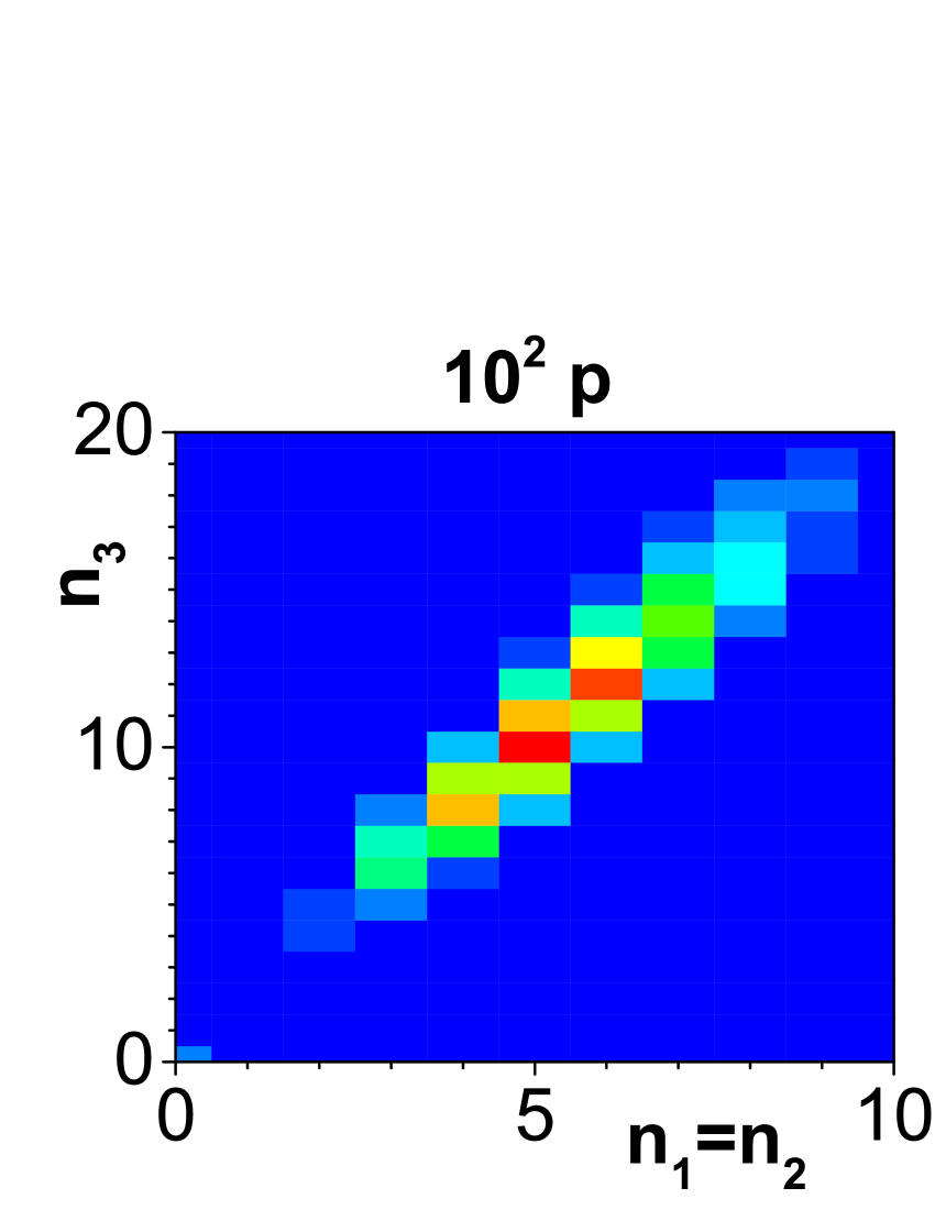
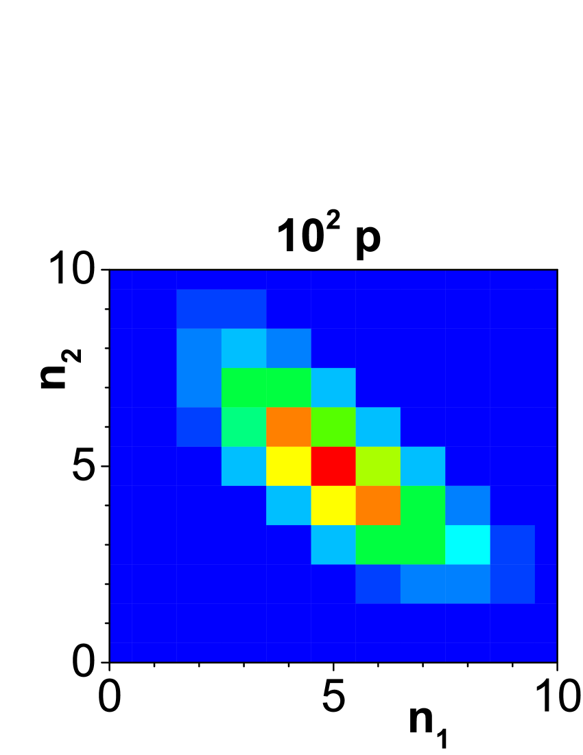
(a)                               (b)

Figure 2: Photon-number distribution $p(n_{1},n_{2},n_{3})$ obtained by ML approach in 2D cuts: (a) $p(n_{1}=n_{2},n_{3})$ and (b) $p(n_{1},n_{2},n_{3}=10)$. Relative errors are better than 1 %.

The experimental 3D optical field was also fitted by the model of two ideal multi-mode Gaussian twin beams ($6.15\pm 0.05$ and $5.95\pm 0.05$ mean photon pairs) and three multi-mode Gaussian noise fields ($0.11\pm 0.02$, $0.07\pm 0.01$ and $0.02\pm 0.01$ mean noise photons). Details are found in Ref. Peřina Jr. et al. (2021a).

By definition, the non-classicality of an optical field means that its quasi-distributions $P_{W}$ of integrated intensities attain negative values for ordering parameters $s>s_{\rm th}$ where $s_{\rm th}$ denotes a threshold value of the ordering parameter. An $s$-ordered quasi-distribution $P_{W,s}({\bf W})$ of integrated intensities for one effective mode in each field is obtained by the following formula Peřina (1991):

$$P_{W,s}({\bf W})=\frac{2^{N}}{(1-s)^{N}}\exp\left(-\frac{2\Sigma{\bf W}}{1-s}\right)\sum_{{\bf n}={\bf 0}}^{\infty}\frac{p({\bf n})}{{\bf n}!}$$

$$\times\left(\frac{s+1}{s-1}\right)^{\Sigma{\bf n}}L_{n_{1}}\left(\frac{4W_{1}}{1-s^{2}}\right)\ldots L_{n_{N}}\left(\frac{4W_{N}}{1-s^{2}}\right);$$ (45)

$L_{k}$ stand for the Laguerre polynomials Morse and Feshbach (1953). We demonstrate the nonclassical behavior of quasi-distribution $P_{W}$ in Fig. 3 where we plot two characteristic cuts for $s=0.02$. Whereas the quasi-distribution $P_{W}$ creates hyperbolic structures in planes $(W_{1},W_{2})$ (for fixed values of intensity $W_{3}$), it forms the structure of rays coming from the point $(W_{1},W_{2},W_{3})=(0,0,0)$ in plane $(W_{1}=W_{2},W_{3})$ that is well known for twin beams Peřina Jr. et al. (2017a).

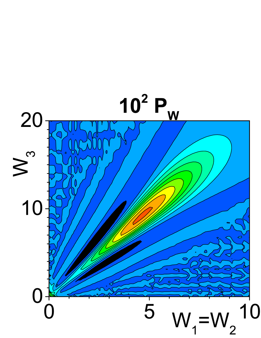
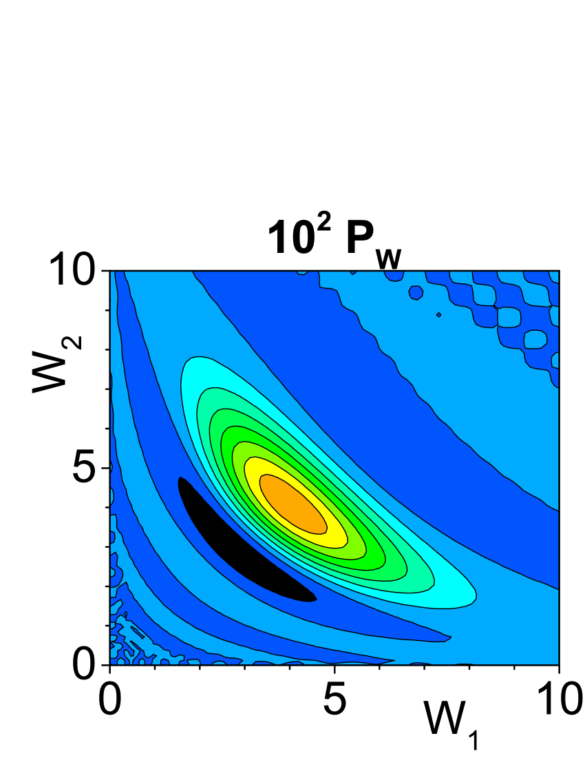
(a)                               (b)

Figure 3: Quasi-distribution $P_{W}(W_{1},W_{2},W_{3})$ of integrated intensities for the ordering parameter $s=0.02$ and the field obtained by ML approach in 2D cuts: (a) $P_{W}(W_{1}=W_{2},W_{3})$ and (b) $P_{W}(W_{1},W_{2},W_{3}=7.9)$.

Now we apply the appropriate NCCa of Sec. II for the introduced $N=3$ dimensional optical field. We address in turn intensity NCCa, probability NCCa and hybrid NCCa.

VII.1 Application of intensity non-classicality criteria

The intensity NCCa containing the lower-order intensity moments are in general stable when applied to the experimental data. This is a consequence of the fact that all experimental data are exploited when the intensity moments are determined. This contrasts with the probability NCCa where only a rather limited amount of the experimental data is used for each NCC. It holds in general for the intensity NCCa that the greater the order of the moments used in a given NCC is the greater the experimental error is. Nevertheless, the NCCa containing the lowest-order intensity moments are usually reliable and very efficient in revealing the non-classicality.

The following intensity NCCa (arranged according to the increasing order of involved intensity moments) derived from the general ones in Eqs. (2), (10) [assuming ${\bf k}=(1,0,0)$, ${\bf l}=(0,1,0)$,${\bf m}=(0,0,1)$], (15) and (16) are capable of identifying the non-classicality of the analyzed field:

$$P^{W,3} = \langle(W_{1}+W_{2}-W_{3})^{2}\rangle<0,$$

$$P^{W,13} = \langle(-W_{1}+W_{2}+W_{3})^{2}(W_{1}+W_{2}-W_{3})^{2}\rangle<0,$$

$$P^{W,23} = \langle(W_{1}-W_{2}+W_{3})^{2}(W_{1}+W_{2}-W_{3})^{2}\rangle<0,$$

$$C_{111}^{120} = \langle W_{1}W_{2}^{2}\rangle\langle W_{1}W_{3}^{2}\rangle-\langle W_{1}W_{2}W_{3}\rangle^{2}<0,$$

$$C_{111}^{210} = \langle W_{1}^{2}W_{2}\rangle\langle W_{2}W_{3}^{2}\rangle-\langle W_{1}W_{2}W_{3}\rangle^{2}<0,$$

$$C_{111}^{002} = \langle W_{1}^{2}W_{2}^{2}\rangle\langle W_{3}^{2}\rangle-\langle W_{1}W_{2}W_{3}\rangle^{2}<0,$$

$$M^{W} = \langle W_{1}^{2}\rangle\langle W_{2}^{2}\rangle\langle W_{3}^{2}\rangle+\langle W_{1}W_{2}\rangle\langle W_{1}W_{3}\rangle\langle W_{2}W_{3}\rangle$$ (46)

$$\mbox{}-\langle W_{1}^{2}\rangle\langle W_{2}W_{3}\rangle^{2}-\langle W_{2}^{2}\rangle\langle W_{1}W_{3}\rangle^{2}$$

$$\mbox{}-\langle W_{3}^{2}\rangle\langle W_{1}W_{2}\rangle^{2}.$$

The polynomial NCC $P^{W,3}$ and the matrix NCC $M^{W}$ provide the greatest values of their NCDs $\tau$ around 0.4, as it follows from the graph in Fig. 4(a).

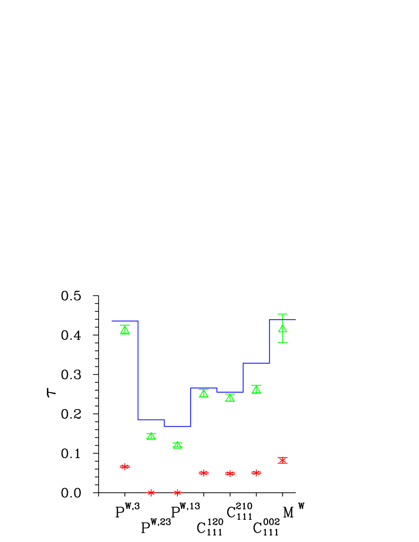
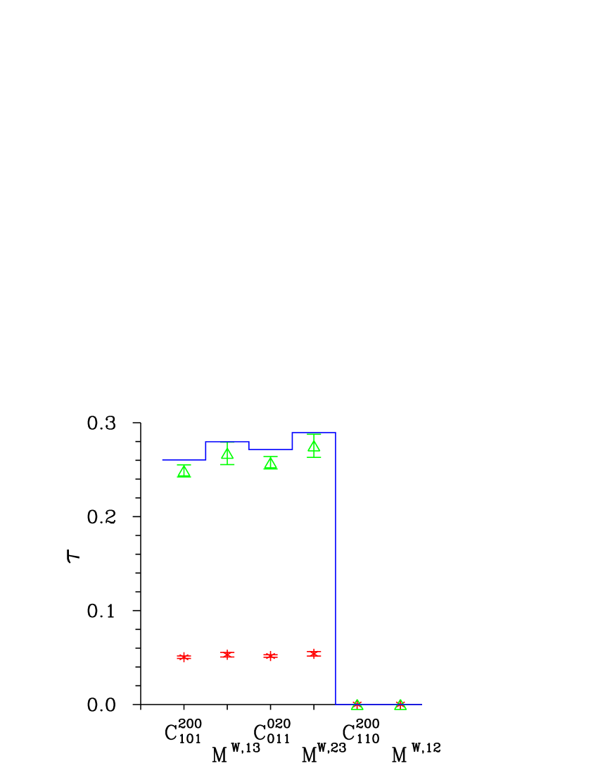
(a)                               (b)

Figure 4: Non-classicality depths $\tau$ for (a) 3D and (b) 2D intensity NCCa. Isolated symbols with error bars are drawn for the experimental photocount histogram (red $\ast$) and field reconstructed by ML approach (green $\triangle$); solid blue curves originate in 3D Gaussian model.

Whereas the matrix NCCa with their complex moment structures are in general successful in revealing the non-classicality, the simple polynomial NCC $P^{W,3}$ complies with the pairwise structure of the analyzed field. The specific type of pairwise correlations in the analyzed field is also detected by the fourth-order Cauchy-Schwarz NCCa $C_{111}^{120}$, $C_{111}^{210}$ and $C_{111}^{002}$ though the values of the corresponding NCDs $\tau$ are smaller. Also the fourth-order polynomial NCCa $P^{W,13}$ and $P^{W,23}$ reveal the non-classicality, owing to the involved term $(W_{1}+W_{2}-W_{3})^{2}$ that they share with the powerful NCC $P^{W,3}$.

More detailed information about the structure of correlations in the analyzed field is obtained when the marginal intensity quasi-distributions are analyzed. The following fourth-order intensity NCCa derived from Eqs. (2) and (10) [assuming ${\bf k}=(0,0)$, ${\bf l}=(1,0)$, ${\bf m}=(0,1)$]

$$C_{101}^{200} = \langle W_{1}^{2}\rangle\langle W_{3}^{2}\rangle-\langle W_{1}W_{3}\rangle^{2}<0,$$

$$C_{110}^{200} = \langle W_{1}^{2}\rangle\langle W_{2}^{2}\rangle-\langle W_{1}W_{2}\rangle^{2}<0,$$

$$C_{011}^{020} = \langle W_{2}^{2}\rangle\langle W_{3}^{2}\rangle-\langle W_{2}W_{3}\rangle^{2}<0,$$

$$M^{W,ij} = \langle W_{i}^{2}\rangle\langle W_{j}^{2}\rangle+2\langle W_{i}\rangle\langle W_{j}\rangle\langle W_{i}W_{j}\rangle$$ (47)

$$\mbox{}-\langle W_{i}\rangle^{2}\langle W_{j}^{2}\rangle-\langle W_{i}^{2}\rangle\langle W_{j}\rangle^{2}-\langle W_{i}W_{j}\rangle^{2},$$

$$\mbox{}\hskip 8.53581pt(i,j)=(1,2),(1,3)(2,3),$$

were found useful for this task. The corresponding NCDs $\tau$ are shown in Fig. 4(b). They reveal strong correlations in the marginal fields (1,3) and (2,3) and no correlation in the marginal field (1,2), in agreement with the structure of the experimentally generated 3D field. Both the matrix and the Cauchy-Schwarz NCCa lead to the values of NCDs $\tau$ around 0.25 for the fields (1,3) and (2,3). The NCDs $\tau$ shown in Fig. 4 indicate slightly greater non-classicality in the field (2,3) compared to the field (1,3).

The values of NCDs $\tau$ in Fig. 4 determined for the model Gaussian field (solid blue curves) are slightly greater than those obtained for the analyzed field reconstructed by the ML approach (green $\triangle$). This reflects the fact that the Gaussian model partly conceals the noise present in the experimental data. For comparison, we plot in Fig. 4 also the values of the NCDs $\tau$ determined directly from the experimental photocount histogram $f$ (red $\ast$). Whereas the NCCa $P^{W,3}$ and $M^{W}$ give the greatest values of NCDs $\tau$ already for the histogram $f$, the NCCa $P^{W,13}$ and $P^{W,23}$ do not indicate the non-classicality in the histogram $f$; they need stronger and less-noisy fields for successful application.

VII.2 Probability non-classicality criteria

In general the probability NCCa are more efficient in revealing the non-classicality Peřina Jr. et al. (2017b, 2020b) compared to their intensity counterparts. The reason is that they test the field non-classicality locally via the probabilities in the field photon-number distribution. On the other hand, the determination of probabilities is more prone to experimental errors compared to the intensity moments whose determination involves all probabilities.

Local non-classicality can be investigated using suitable probability NCCa containing only the probabilities from small regions. We illustrate this approach by defining the probability NCCa $C^{p}$ and $M^{p}$ that are in fact specific groups of the Cauchy-Schwarz and the matrix NCCa from Eqs. (19) and (20):

$$C^{p}_{\bf n} = \min_{{\bf m},|{\bf m}-{\bf n}|\leq 1}\{\bar{C}_{\bf n}^{\bf m}\}<0,$$

$$M^{p}_{\bf n} = \min_{{\bf k},{\bf l},|{\bf k}-{\bf n}|\leq 1,|{\bf l}-{\bf n}|\leq 1}\{\bar{M}_{\bf kln}\}<0,$$ (48)

where $|{\bf m}-{\bf n}|\leq 1$ stands for the simultaneous conditions $|m_{i}-n_{i}|\leq 1$ for $i=1,2,3$. We also consider the probability polynomial NCCa $E^{p,13}$ derived from the intensity NCCa in Eq. (12) because these NCCa are efficient in identifying the non-classicality originating in photon pairing Peřina Jr. et al. (2020a):

$$E^{p,13}_{\bf n} = \frac{n_{1}+2}{n_{3}+1}p(n_{1}+2,n_{2},n_{3})+\frac{n_{3}+2}{n_{1}+1}p(n_{1},n_{2},n_{3}+2)$$ (49)

$$\mbox{}-2p(n_{1}+1,n_{2},n_{3}+1)<0.$$

The cuts of the probability NCCa $C^{p}$, $M^{p}$ and $E^{p,13}$ plotted in Fig. 5, that correspond to the cuts of the photon-number distribution $p$ in Fig. 2, reveal that the greatest values of the NCDs $\tau$ occur in the central part of the 3D photon-number distribution $p$. These values drop down as we move towards the photon-number distribution tails.

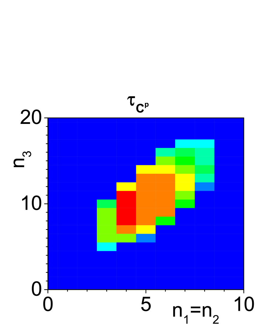
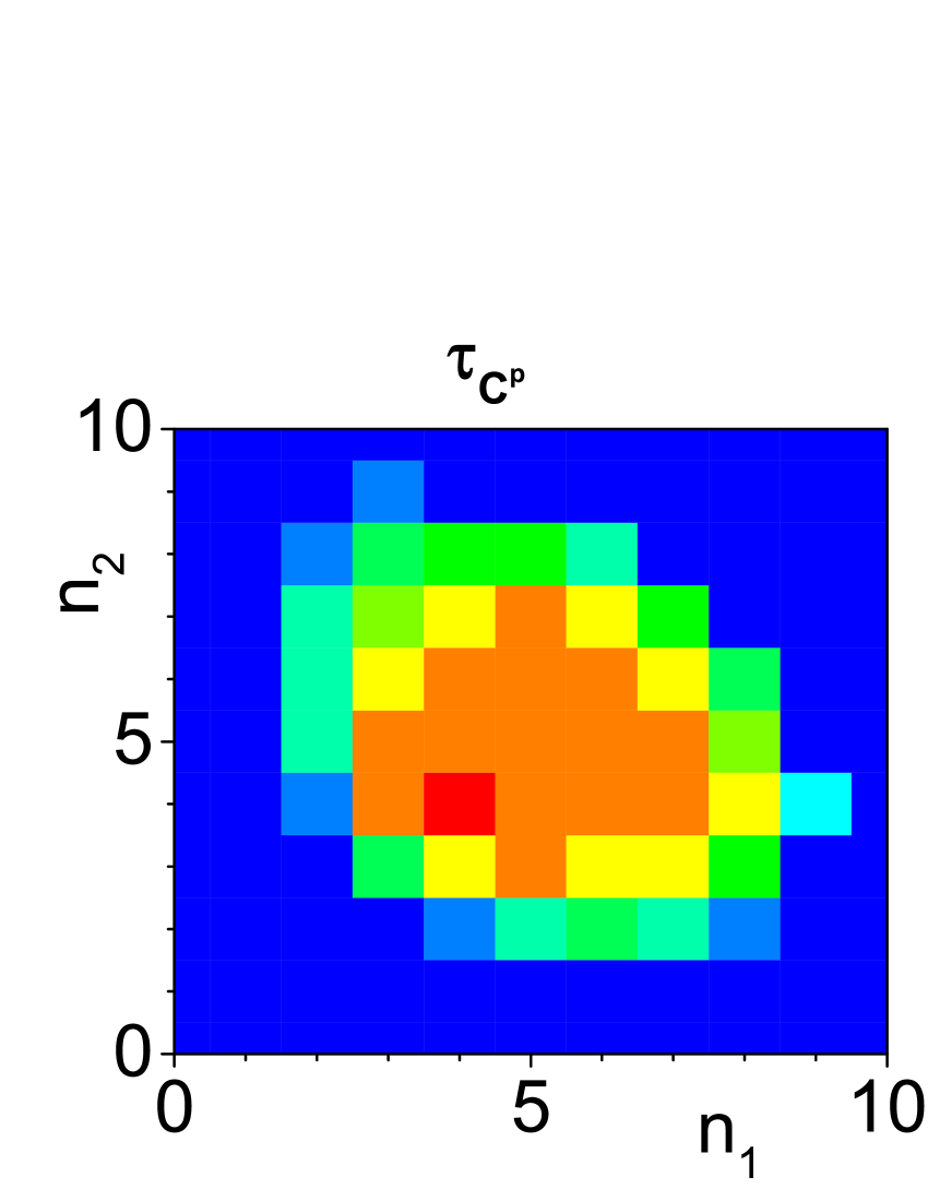
(a)                               (b)

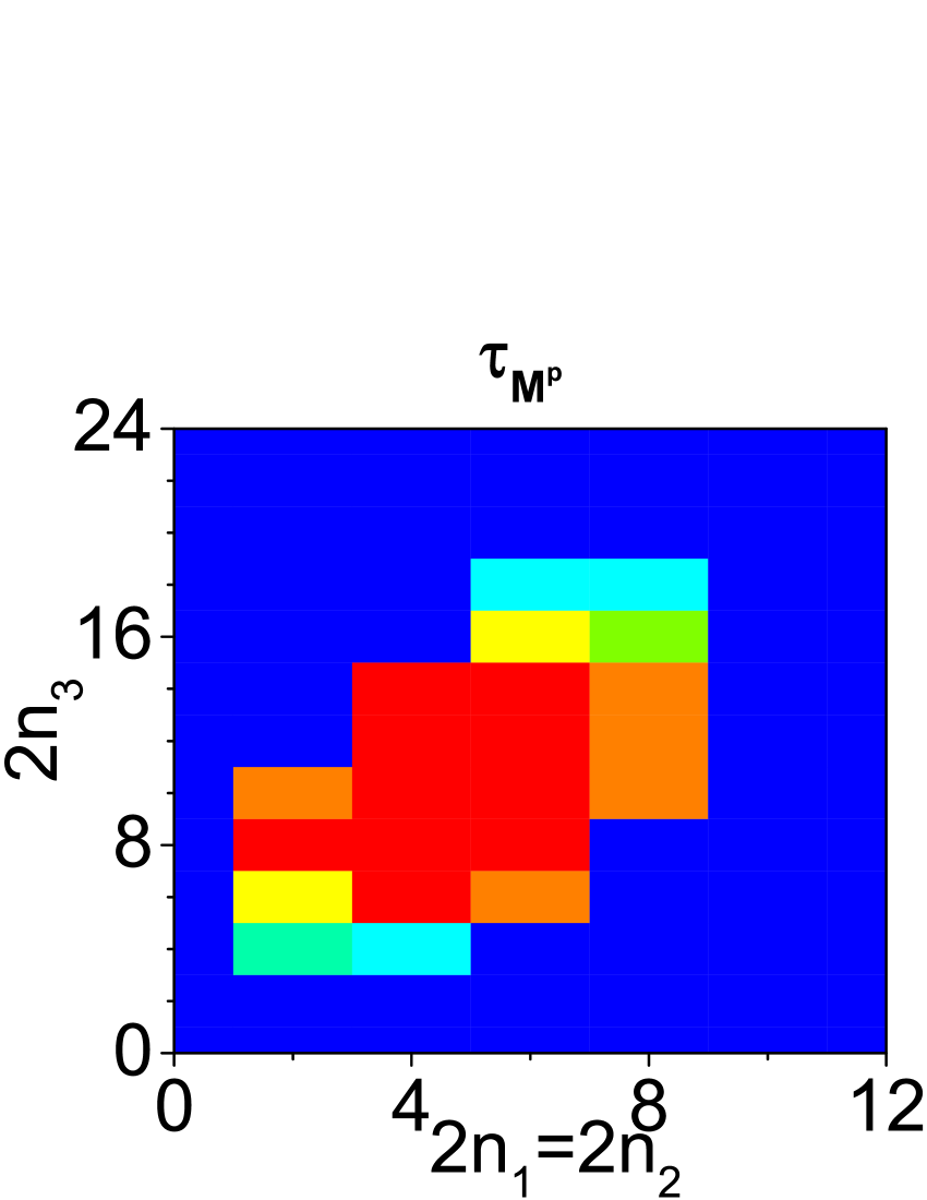
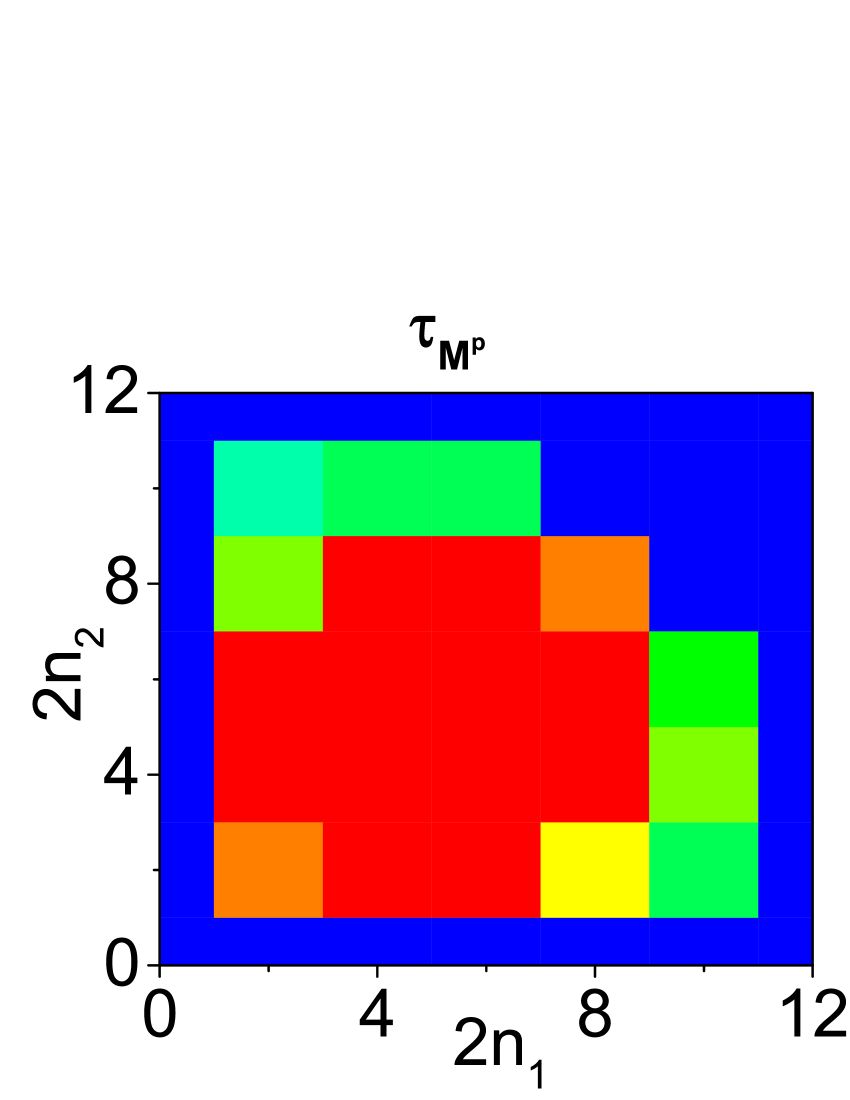
(c)                               (d)

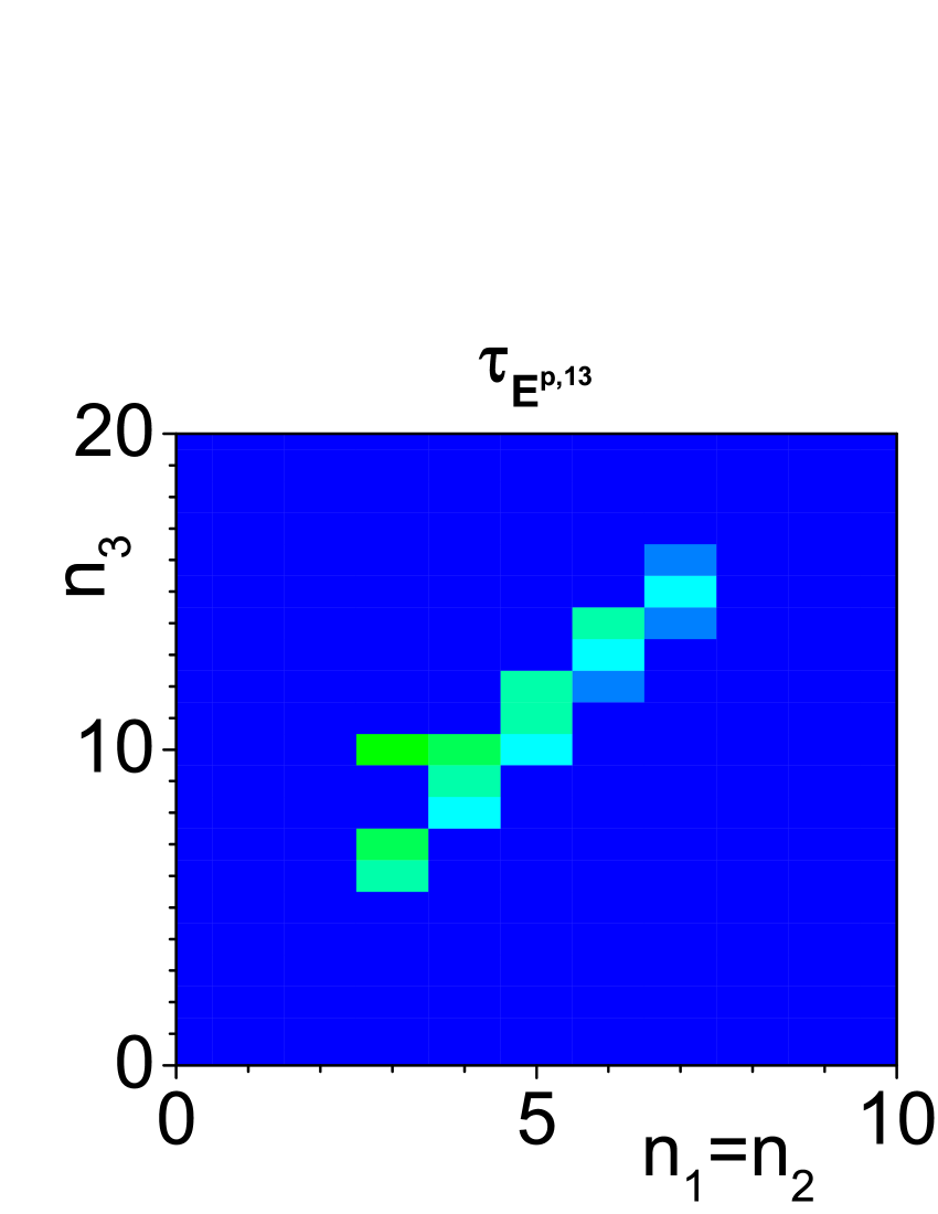
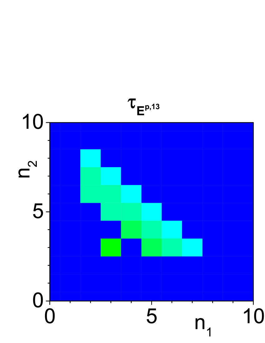
(e)                               (f)

Figure 5: Non-classicality depths $\tau$ for probability NCCa (a,b) $C^{p}$, (c,d) $M^{p}$ and (e,f) $E^{p,13}$ as they depend on photon numbers $n_{1}$, $n_{2}$ and $n_{3}$ in 2D cuts; $n_{3}=10$ in (b,f), $2n_{3}=10$ in (d). Only the NCCa for which the mean value of the used probabilities is greater than 0.001 are taken into account. Relative errors in (a,b), (c,d) and (e,f) are in turn better than 3 %, 8 % and 2 %.

As documented in the graphs of Fig. 5 the matrix NCCa $M^{p}$ perform the best followed by the Cauchy-Schwarz NCCa $C^{p}$; both types of NCCa indicate the greatest values of NCDs $\tau$ close to 0.5. The polynomial NCCa $E^{p,13}$ give the maximal values of NCDs $\tau$ only around 0.3, which is a consequence of their structure that is sensitive only to photon pairs in the field 13. Comparing the probability NCCa with their intensity counterparts, the NCDs $\tau$ are greater by around 0.1 (0.2) for the matrix (Cauchy-Schwarz) NCCa.

Contrary to the probability NCCa discussed above and containing finite numbers of probabilities, the Hillery criteria $H_{1}$ and $H_{2}$ from Eqs. (29) and (32) contain infinite numbers of probabilities. However, they did not perform well when analyzing the 3D field reconstructed by the ML approach: Only the NCC $H_{2}$ applied in 3D provided non-zero value of NCD $\tau=0.020\pm 0.001$. On the other hand, for the model Gaussian field the NCCa $H_{2}$ revealed the non-classicality of 3D field [$\tau=0.211$] as well as the marginal 2D fields (1,3) [$\tau=0.015$] and (2,3) [$\tau=0.050$]. This indicates that the Hillery criteria are not suitable for identifying the non-classicality in experimental photon-number distributions because of the inevitable noise.

VII.3 Hybrid non-classicality criteria

The hybrid criteria that contain both probabilities and intensity moments represent in certain sense a bridge between the intensity and probability NCCa. Their expected performance in revealing the non-classicality and resistance against the experimental errors lie in the middle. On one side they are less efficient but more stable than the probability NCCa, on the other side they are more powerful but less stable than the intensity NCCa. With their help, we can monitor specific aspects of the non-classicality of the analyzed fields including the experimental issues.

To demonstrate their properties, we first consider the following Cauchy-Schwarz and the matrix NCCa derived from Eq. (26) [assuming ${\bf m}_{W}=(0,2)$, ${\bf n}_{W}=(1,1)$, ${\bf m}_{p}=(n_{k}-m_{k})$, ${\bf n}_{p}=(n_{k})$] and Eq. (10) converted partly into the probability NCCa via the mapping in Eq. (24) [assuming ${\bf k}=(0,0,n_{k})$, ${\bf l}=(1,0,n_{k})$, ${\bf m}=(0,1,n_{k})$]:

$$C^{pW,k}_{n_{k},m_{k}} = \frac{(n_{k}+m_{k})!(n_{k}-m_{k})!}{(n_{k}!)^{2}}\langle W_{i}^{2}\rangle_{p_{k}(n_{k}+m_{k})}$$

$$\mbox{}\times\langle W_{j}^{2}\rangle_{p_{k}(n_{k}-m_{k})}-\langle W_{i}W_{j}\rangle_{p_{k}(n_{k})}^{2}<0,$$

$$M^{pW,k}_{n_{k}} = \langle 1\rangle_{p_{k}(2n_{k})}\langle W_{i}^{2}\rangle_{p_{k}(2n_{k})}\langle W_{j}^{2}\rangle_{p_{k}(2n_{k})}$$ (50)

$$\mbox{}+2\langle W_{i}\rangle_{p_{k}(2n_{k})}\langle W_{j}\rangle_{p_{k}(2n_{k})}\langle W_{i}W_{j}\rangle_{p_{k}(2n_{k})}$$

$$\mbox{}-\langle W_{i}\rangle^{2}_{p_{k}(2n_{k})}\langle W_{j}^{2}\rangle_{p_{k}(2n_{k})}-\langle W_{i}^{2}\rangle_{p_{k}(2n_{k})}\langle W_{j}\rangle^{2}_{p_{k}(2n_{k})}$$

$$\mbox{}-\langle 1\rangle_{p_{k}(2n_{k})}\langle W_{i}W_{j}\rangle_{p_{k}(2n_{k})}^{2}<0,$$

$$(i,j,k)=(1,2,3),(2,3,1),(3,1,2).$$

The Cauchy-Schwarz NCC $C^{pW,k}$ for $m_{k}=0$ represents a 2D intensity NCC for the field ($i,j$) conditioned by the detection of $n_{k}$ photons in field $k$. The values of NCDs $\tau$ for the field (2,3) lie around 0.35, as documented in Fig. 6(a).

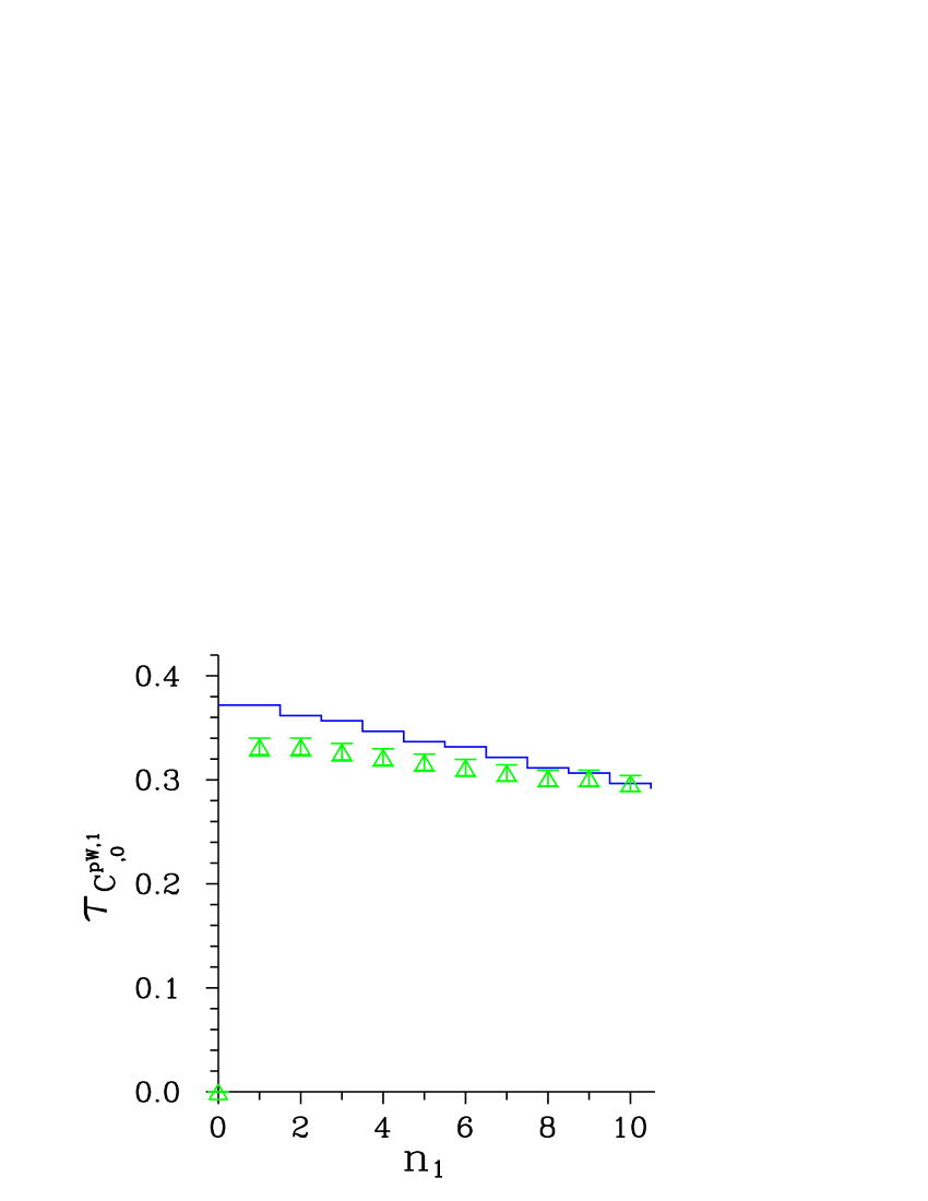
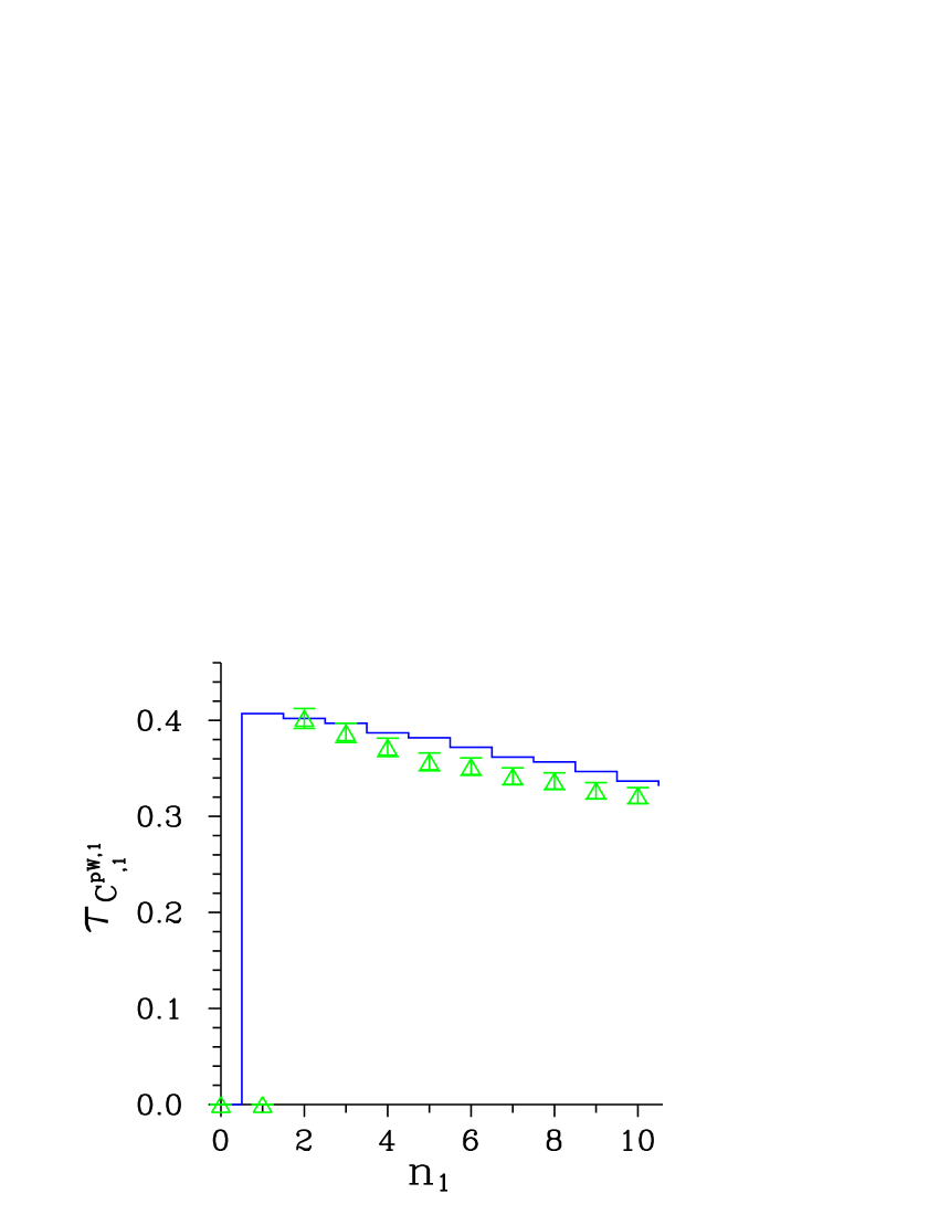
(a)                               (b)

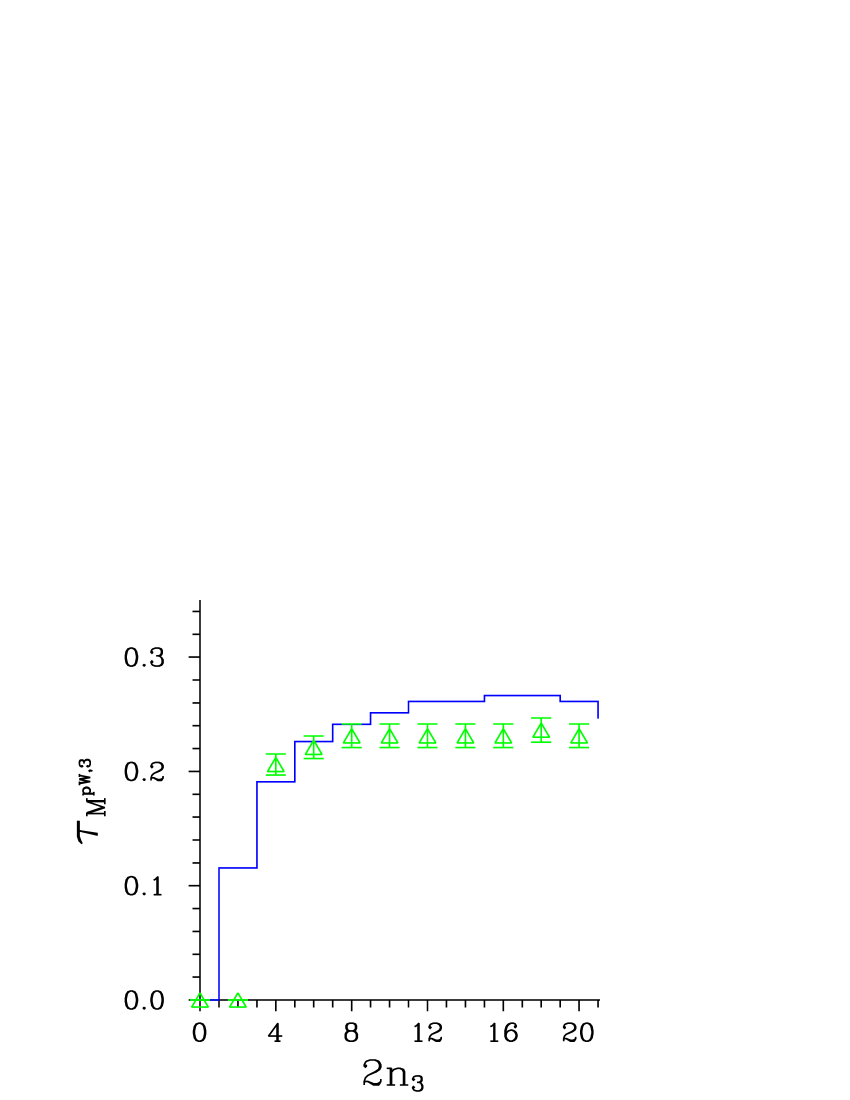
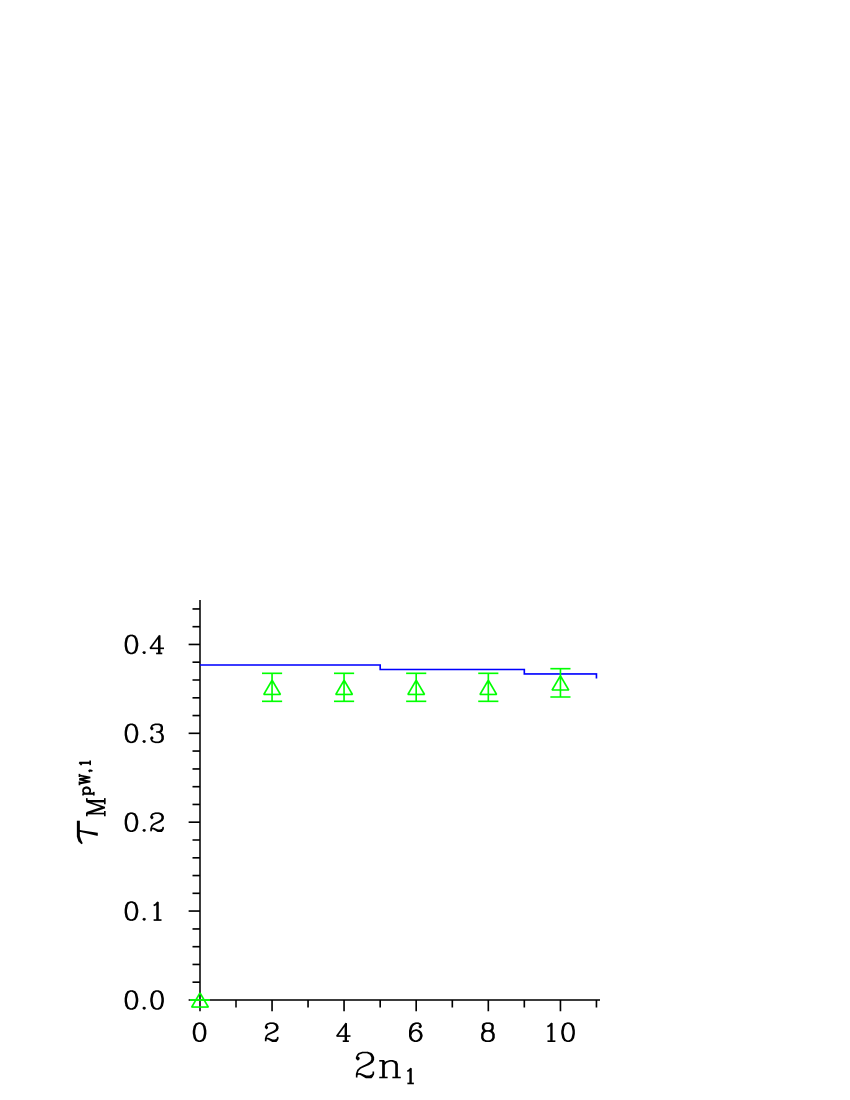
(c)                               (d)

Figure 6: Non-classicality depths $\tau$ for hybrid NCCa (a) $C^{pW,1}_{,0}$, (b) $C^{pW,1}_{,1}$, (c) $M^{pW,3}$, and (c) $M^{pW,1}$ as they depend on the corresponding photon numbers $n_{1}$, $2n_{1}$ and $2n_{3}$. Isolated symbols with error bars are plotted for the field reconstructed by ML approach (green $\triangle$); solid blue curves originate in 3D Gaussian model.

They are greater by around 0.1 compared to the value $\tau=0.257\pm 0.007$ for the NCC $C^{020}_{011}$ of the marginal field (2,3). This is explained as follows. The conditional fields occur in the decomposition of the marginal field (2,3) (with appropriate weights). Composing the marginal field from its conditional constituents we partly conceal the non-classicality. The Cauchy-Schwarz NCC $C^{pW,k}$ in its general form ($m_{k}\neq 0$) involves the moments of three 2D fields ($i,j$) conditioned by the detection of $n_{k}-m_{k}$, $n_{k}$ and $n_{k}+m_{k}$ photons in field $k$. In its general form it allows to reach even greater values of the NCDs $\tau$, as demonstrated in Fig. 6(b).

Two limiting cases of the behavior of the non-classicality when composing the field from its conditional constituents are shown in Figs. 6(c,d) considering the matrix NCCa $M^{pW,1}$ and $M^{pW,3}$ from Eq. (48). Whereas the hybrid NCCa $M^{pW,3}$ indicate the NCDs $\tau$ around 0.22 for the conditional fields (1,2) in Fig. 6(c), the marginal field (1,2) is classical ($M^{W,23}=0$). On the other hand, the hybrid NCCa $M^{pW,1}$ assign the NCDs $\tau$ around 0.35 for the conditional fields (2,3) and similar value $\tau=0.28\pm 0.01$ is obtained for the marginal field (2,3) applying the NCC $M^{W,23}$. We note that, in Fig. 6, similarly as in the case of intensity NCCa, the values of NCDs $\tau$ obtained from the model Gaussian field are slightly greater than those characterizing the field reconstructed by the ML approach.

As another example, we consider the following hybrid Cauchy-Schwarz and matrix criteria $C^{Wp,i}$ and $M^{Wp,i}$ obtained from Eq. (26) [assuming ${\bf m}_{W}=(0)$, ${\bf n}_{W}=(1)$, ${\bf m}_{p}={\bf n}_{p}=(n_{j},n_{k})$] and Eq. (10) converted into the probability NCCa [assuming ${\bf k}=(0,n_{j},n_{k})$, ${\bf l}=(1,n_{j},n_{k})$, ${\bf m}=(2,n_{j},n_{k})$] using the mapping in Eq. (24):

$$C^{Wp,i}_{n_{j},n_{k}} = \langle W_{i}^{2}\rangle_{p_{jk}(n_{j},n_{k})}\langle 1\rangle_{p_{jk}(n_{j},n_{k})}$$

$$\mbox{}-\langle W_{i}\rangle_{p_{jk}(n_{j},n_{k})}^{2}<0,$$

$$M^{Wp,i}_{n_{j},n_{k}} = \langle 1\rangle_{p_{jk}(2n_{j},2n_{k})}\langle W_{i}^{2}\rangle_{p_{jk}(2n_{j},2n_{k})}\langle W_{i}^{4}\rangle_{p_{jk}(2n_{j},2n_{k})}$$ (51)

$$\mbox{}+2\langle W_{i}\rangle_{p_{jk}(2n_{j},2n_{k})}\langle W_{i}^{2}\rangle_{p_{jk}(2n_{j},2n_{k})}\langle W_{i}^{3}\rangle_{p_{jk}(2n_{j},2n_{k})}$$

$$\mbox{}-\langle 1\rangle_{p_{jk}(2n_{j},2n_{k})}\langle W_{i}^{3}\rangle_{p_{jk}(2n_{j},2n_{k})}^{2}-\langle W_{i}\rangle_{p_{jk}(2n_{j},2n_{k})}^{2}$$

$$\mbox{}\times\langle W_{i}^{4}\rangle_{p_{jk}(2n_{j},2n_{k})}-\langle W_{i}^{2}\rangle_{p_{jk}(2n_{j},2n_{k})}^{3}<0,$$

$$(i,j,k)=(1,2,3),(2,3,1),(3,1,2).$$

The hybrid NCCa in Eq. (51) represent 1D intensity NCCa for the field $i$ conditioned by simultaneous detection of $n_{j}$ photons in field $j$ and $n_{k}$ photons in field $k$.

For the analyzed 3D field, the conditional fields 1 are less nonclassical than the conditional fields 3, as evidenced in the graphs of Fig. 7 showing the NCDs $\tau$ of the NCCa $C^{Wp,1}$ and $M^{Wp,1}$ belonging to conditional fields 1 and $C^{Wp,3}$ and $M^{Wp,3}$ quantifying the non-classicality of conditional fields 3. The NCCa $C^{Wp,1}$ and $M^{Wp,1}$ ($C^{Wp,3}$ and $M^{Wp,3}$) assign the values of NCDs $\tau$ around 0.2 (0.3) for the conditional fields 1 (3).

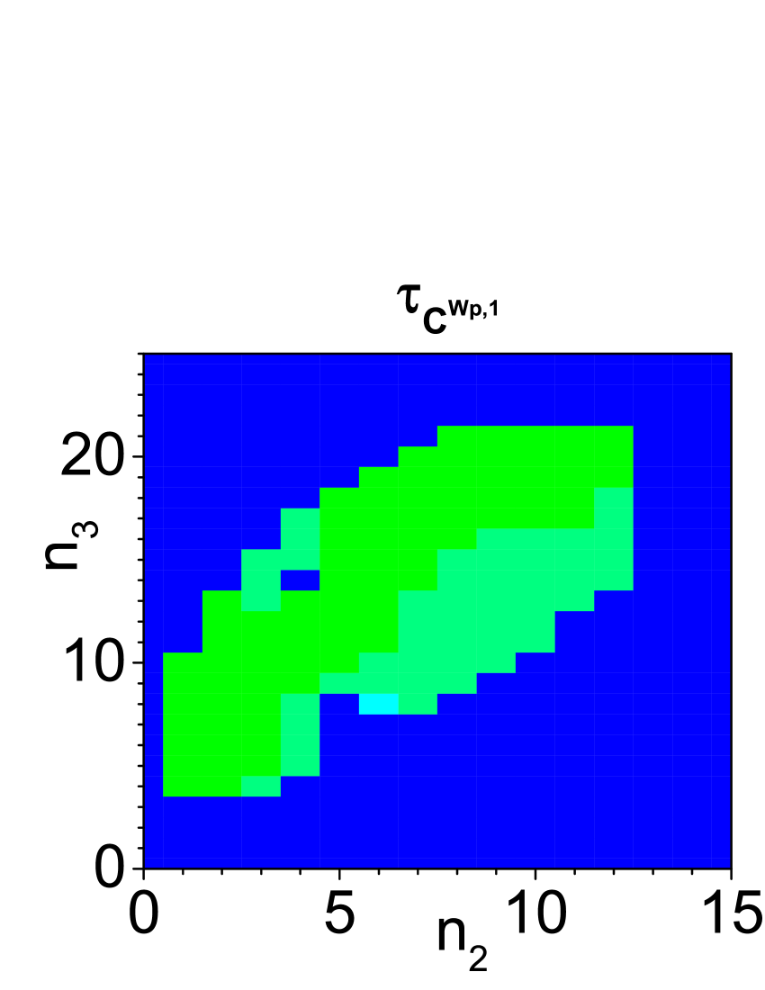
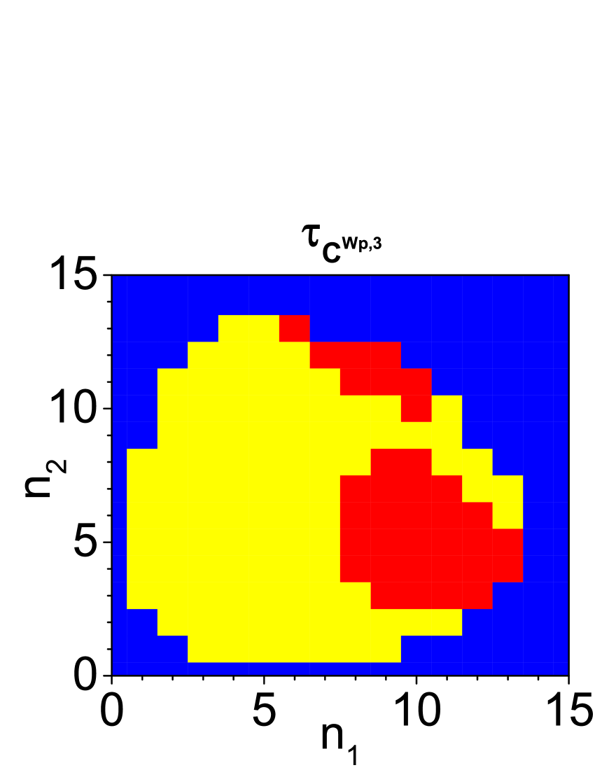
(a)                               (b)

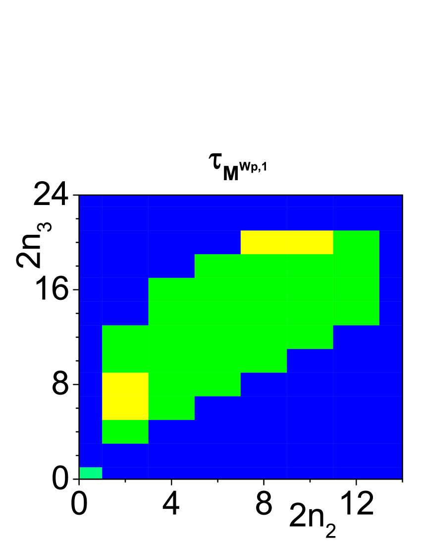
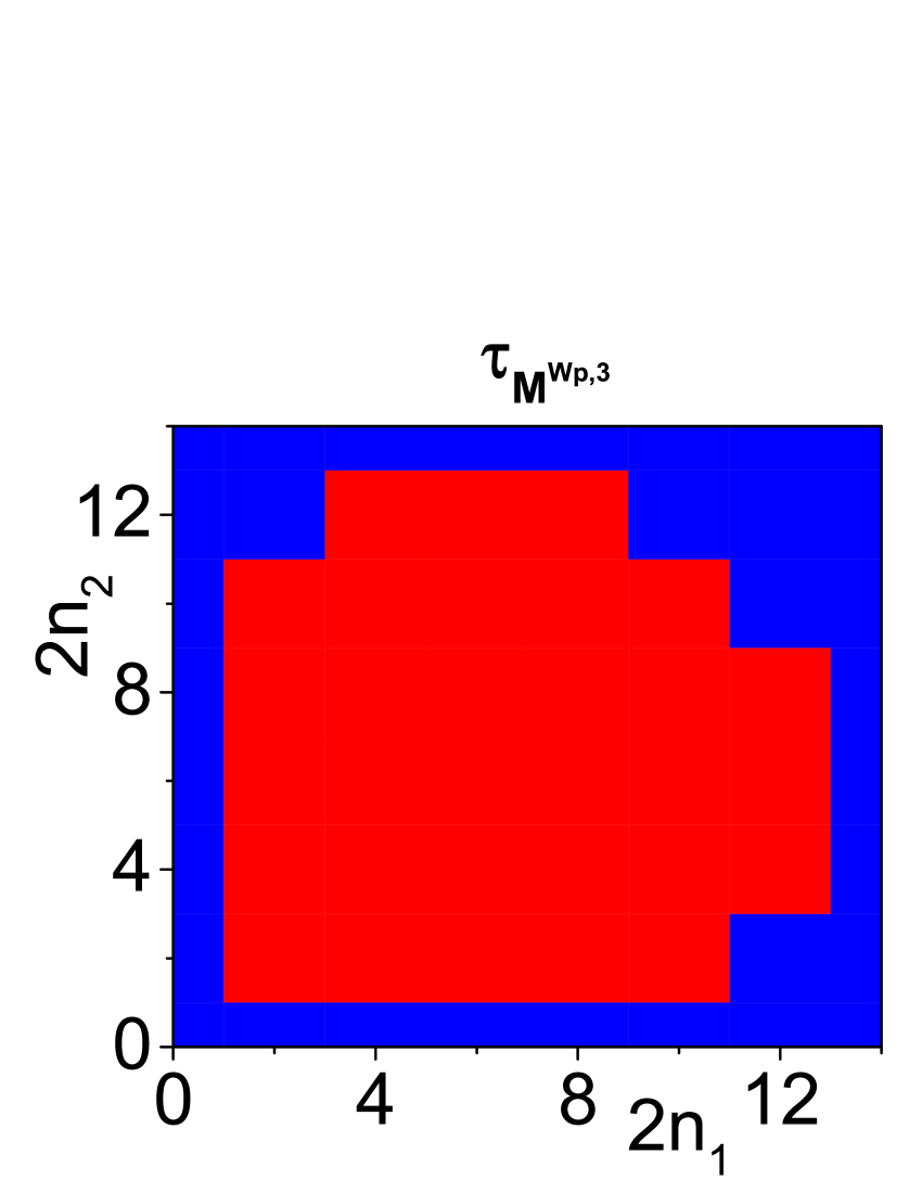
(c)                               (d)

Figure 7: Non-classicality depths $\tau$ for hybrid NCCa (a) $C^{Wp,1}$, (b) $C^{Wp,3}$, (c) $M^{Wp,1}$, and (c) $M^{Wp,3}$ as they depend on the corresponding photon numbers $n_{1}$, $n_{2}$, $n_{3}$, $2n_{1}$, $2n_{2}$, and $2n_{3}$. Relative errors in (a,b) [(c,d)] are better than 3 % [15 %].

This asymmetry originates in the structure of the analyzed 3D field. Whereas the non-classicality in conditional fields 1 is caused by photon pairs residing in the fields 13 and 23 whose numbers are chosen by ’two-step’ post-selection based on the detection of given numbers of photons in the fields 2 and 3, the non-classicality of conditional fields 3 has its origin in both types of photon pairs (residing in fields 13 and 23) and independent post-selections requiring the detection of given numbers of photons in the fields 1 and 2.

VIII Conclusions

Using the Cauchy-Schwarz inequality, nonnegative quadratic forms, the majorization theory and nonnegative polynomials we have formulated large groups of non-classicality criteria for general $N$-dimensional optical fields. The non-classicality criteria were written in intensity moments, probabilities of photon-number distributions and a specific hybrid form that simultaneously includes both intensity moments and probabilities. The derived non-classicality criteria were decomposed into the simplest building blocks and then mutually compared. The fundamental non-classicality criteria suitable for application were identified. As a special example, an $N$-dimensional form of the Hillery non-classicality criteria was derived.

Discussing the transformation of intensity moments and photon-number distributions between different field-operator orderings, quantification of the non-classicality based on these criteria and using the non-classicality depth was accomplished.

The properties as well as the performance of the derived non-classicality criteria were demonstrated considering an experimental 3-dimensional optical field containing two types of photon pairs. It was shown that the intensity non-classicality criteria are both efficient in revealing the non-classicality and robust with respect to experimental errors. The ability of the probability non-classicality criteria to provide insight into the distribution of non-classicality across the profile of photon-number distribution was demonstrated. The hybrid non-classicality criteria were presented as a useful alternative to the intensity and probability non-classicality criteria.

The analyzed experimental example proved that the non-classicality criteria represent a very powerful tool in identifying and quantifying the non-classicality in its various forms. The derived non-classicality criteria are versatile and as such they can be successfully applied to any optical field.