The dynamics of representation learning in shallow, non-linear autoencoders

Abstract

Autoencoders are the simplest neural network for unsupervised learning, and thus an ideal framework for studying feature learning. While a detailed understanding of the dynamics of linear autoencoders has recently been obtained, the study of non-linear autoencoders has been hindered by the technical difficulty of handling training data with non-trivial correlations – a fundamental prerequisite for feature extraction. Here, we study the dynamics of feature learning in non-linear, shallow autoencoders. We derive a set of asymptotically exact equations that describe the generalisation dynamics of autoencoders trained with stochastic gradient descent (SGD) in the limit of high-dimensional inputs. These equations reveal that autoencoders learn the leading principal components of their inputs sequentially. An analysis of the long-time dynamics explains the failure of sigmoidal autoencoders to learn with tied weights, and highlights the importance of training the bias in ReLU autoencoders. Building on previous results for linear networks, we analyse a modification of the vanilla SGD algorithm which allows learning of the exact principal components. Finally, we show that our equations accurately describe the generalisation dynamics of non-linear autoencoders trained on realistic datasets such as CIFAR10, thus establishing shallow autoencoders as an instance of the recently observed Gaussian universality.

1 Introduction

Autoencoders are a class of neural networks trained to reconstruct their inputs by minimising the distance between an input $\boldsymbol{x}\in\mathcal{X}$, and the network output $\hat{\boldsymbol{x}}\in\mathcal{X}$. The key idea for learning good features with autoencoders is to make the intermediate layer in the middle of the network (significantly) smaller than the input dimension. This “bottleneck” forces the network to develop a compressed representation of its inputs, together with an encoder and a decoder. Autoencoders of this type are called undercomplete, see fig. 1, and provide an ideal framework to study feature learning, which appears to be a key property of deep learning, yet remains poorly understood from a theoretical point of view.

How well can shallow autoencoders with a single hidden layer of neurons perform on a reconstruction task? For linear autoencoders, Eckart & Young (1936) established that the optimal reconstruction error is obtained by a network whose weights are given by (a rotation of) the $K$ leading principal components of the data, i.e. the $K$ leading eigenvectors of the input covariance matrix. The reconstruction error of such a network is therefore called the PCA error. How linear autoencoders learn these components when trained using stochastic gradient descent (SGD) was first studied by Bourlard & Kamp (1988) and Baldi & Hornik (1989). A series of recent work analysed linear autoencoders in more detail, focusing on the loss landscape (Kunin et al., 2019), the convergence and implicit bias of SGD dynamics (Pretorius et al., 2018; Saxe et al., 2019; Nguyen et al., 2019), and on recovering the exact principal components (Gidel et al., 2019; Bao et al., 2020; Oftadeh et al., 2020).

Adding a non-linearity to autoencoders is a key step on the way to more realistic models of neural networks, which crucially rely on non-linearities in their hidden layers to extract good features from data. On the other hand, non-linearities pose a challenge for theoretical analysis. In the context of high-dimensional models of learning, an additional complication arises from analysing non-linear models trained on inputs with non-trivial correlations, which are a fundamental prerequisite for unsupervised learning. The first step in this direction was taken by Nguyen (2021), who analysed overcomplete autoencoders where the number of hidden neurons grows polynomially with the input dimension, focusing on the special case of weight-tied autoencoders, where encoder and decoder have the same weights.

Here, we leverage recent developments in the analysis of supervised learning on complex input distributions to study the learning dynamics of undercomplete, non-linear autoencoders with both tied and untied weights. While their reconstruction error is also limited by the PCA reconstruction error (Bourlard & Kamp, 1988; Baldi & Hornik, 1989), we will see that their learning dynamics is rich and raises a series of questions: can non-linear AE trained with SGD reach the PCA error, and if so, how do they do it? How do the representations they learn depend on the architecture of the network, or the learning rule used to train them?

We describe our setup in detail in section 2. Our main contributions can be summarised as follows:

1. We derive a set of asymptotically exact equations that describe the generalisation dynamics of shallow, non-linear autoencoders trained using online stochastic gradient descent (SGD) (section 3.1);

2. Using these equations, we show how autoencoders learn important features of their data sequentially (3.2); we analyse the long-time dynamics of learning and highlight the importance of untying the weights of decoder and encoder (3.3); and we show that training the biases is necessary for ReLU autoencoders; (3.4)

3. We illustrate how a modification of vanilla SGD breaking the rotational symmetry of neurons yields the exact principal components of the data (section 3.5);

4. We finally show that the equations also capture the learning dynamics of non-linear autoencoders trained on more realistic datasets such as CIFAR10 with great accuracy, and discuss connections with recent results on Gaussian universality in neural network models in section 4.

Reproducibility

We provide code to solve the dynamical equations of section 3.1 and to reproduce our plots at https://github.com/mariaref/NonLinearShallowAE.

2 Setup

Architecture

We study the performance and learning dynamics of shallow non-linear autoencoders with $K$ neurons in the hidden layer. Given a $D$-dimensional input $\boldsymbol{x}=(x_{i})$, the output of the autoencoder is given by

$$\hat{x}_{i}=\sum_{k}^{K}v_{i}^{k}g\left(\lambda^{k}\right),\qquad\lambda^{k}\equiv\frac{\boldsymbol{w}^{k}\boldsymbol{x}}{\sqrt{D}}$$ (1)

where $\boldsymbol{w}^{k},\boldsymbol{v}^{k}\in\mathbb{R}^{D}$ are the encoder and decoder weight of the $k$th hidden neuron, resp., and $g(\cdot)$ is a non-linear function. We study this model in the thermodynamic limit where we let the input dimension $D\!\to\!\infty$ while keeping the number of hidden neurons $K$ finite, as shown in fig. 1 (a). The performance of a given autoencoder is measured by the population reconstruction mean-squared error,

$$\operatorname{\sf pmse}\equiv\frac{1}{D}\sum_{i}\mathbb{E}(x_{i}-\hat{x}_{i})^{2},$$ (2)

where the expectation $\mathbb{E}\,$ is taken with respect to the data distribution. Nguyen (2021) analysed shallow autoencoders in a complementary mean-field limit, where the number of hidden neurons $K$ grows polynomially with the input dimension. Here, by focusing on the case $K\!<\!D$, we study the case where the hidden layer is a bottleneck. Nguyen (2021) considers tied autoencoders, where a single set of weights is shared between encoder and decoder, $w^{k}\!=\!v^{k}$. We will see in section 3.3 that untying the weights is critical to achieve a non-trivial reconstruction error in the regime $K<D$.

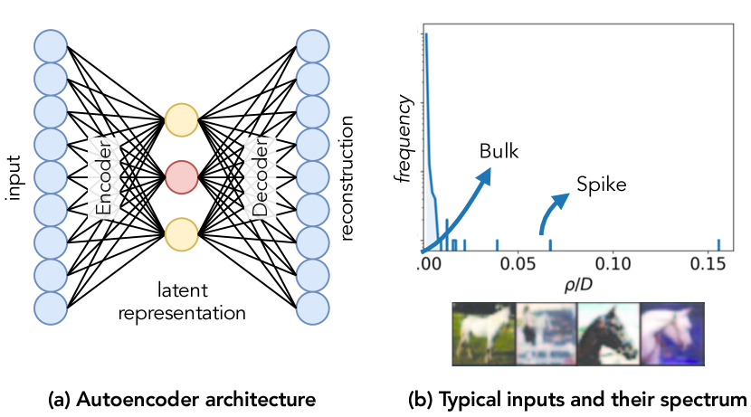
Figure 1: Shallow autoencoders and their inputs (a) We analyse two-layer autoencoders with non-linear activation function in the hidden layer. (b) Top: Rescaled eigenvalues of the covariance matrix of inputs drawn from the spiked Wishart model in eq. 3, which can be divided into a bulk and a finite number of outliers. Bottom: example inputs drawn from CIFAR10 (Krizhevsky et al., 2009), a benchmark data set we use for our experiments with realistic data in section 4.

Data model

We derive our theoretical results for inputs drawn from a spiked Wishart model (Wishart, 1928; Potters & Bouchaud, 2020), which has been widely studied in statistics to analyse the performance of unsupervised learning algorithms. In this model, inputs are sampled according to

$$\boldsymbol{x}_{\mu}=\text{{A}}\boldsymbol{c}_{\mu}+\sqrt{\sigma}\boldsymbol{\xi}_{\mu},$$ (3)

where $\mu$ is an index that runs over the inputs in the training set, $\boldsymbol{\xi}_{\mu}$ is a $D$-dimensional vector whose elements are drawn i.i.d. from a standard Gaussian distribution and $\sigma\!>\!0$. The matrix $\text{{A}}\!\in\!\mathbb{R}^{D\times M}$ has elements of order $\order{1}$ and is fixed for all inputs, while we sample $\boldsymbol{c}_{\mu}\!\in\!\mathbb{R}^{M}$ from some distribution. Different choices for A and the distribution of $\boldsymbol{c}$ allow modelling of Gaussian mixtures, sparse codes, and non-negative sparse coding.

Spectral properties of the inputs

The spectrum of the covariance of the inputs is determined by A and $\boldsymbol{c}$. It governs the dynamics and the performance of autoencoders (by construction, we have $\mathbb{E}\,x_{i}\!=\!0$). If we set $\boldsymbol{c}_{\mu}\!=\!0$ in eq. 3, inputs would be i.i.d. Gaussian vectors with an average covariance of $\mathbb{E}x_{i}x_{j}\!=\!\delta_{ij}$, where $\delta_{ij}$ is the Kronecker delta. The empirical covariance matrix of a finite data set with $P\!\sim\!\order{D}$ samples has a Marchenko–Pastur distribution with a scale controlled by $\sigma$ (Marchenko & Pastur, 1967; Potters & Bouchaud, 2020). By sampling the $m$th element of $\boldsymbol{c}$ as $c_{m}\!\sim\!\mathcal{N}(0,\tilde{\rho}_{m})$, we ensure that the input-input covariance has $M$ eigenvalues $\rho_{m}\!=\!D\tilde{\rho}_{m}$ with the columns of A as the corresponding eigenvectors. The remaining $D\!-\!M$ eigenvalues of the empirical covariance, i.e. the bulk, still follow the Marchenko-Pastur distribution. We further ensure that the reconstruction task for the autoencoder is well-posed by letting the outlier eigenvalues scale as $\rho_{m}\!\sim\!\order{D}$ (or $\tilde{\rho}_{m}\!\sim\!\order{1}$), resulting in spectra such as the one shown in fig. 1(b). If the largest eigenvalues were of order one, an autoencoder with a finite number of neurons $K$ could not obtain a $\operatorname{\sf pmse}$ better than random guessing as the input dimension $D\!\to\!\infty$.

Training

We train the autoencoder on the quadratic error in the one-pass (or online) limit of stochastic gradient descent (SGD), where a previously unseen input $\boldsymbol{x}$ is presented to the network at each step of SGD. This limit is extensively used to analyse the dynamics of non-linear networks for both supervised and unsupervised learning, and it has been shown experimentally to capture the dynamics of deep networks trained with data augmentation well (Nakkiran et al., 2021). The SGD weight increments for the network parameters are then given by:

$$\differential w_{i}^{k} =-\frac{\eta_{W}}{D}\left(\frac{1}{\sqrt{D}}\sum_{j}v_{j}^{k}\Delta_{j}g^{\prime}(\lambda^{k})x_{i}\right)-\frac{\kappa}{D}w_{i}^{k},$$ (4a)

$$\differential v_{i}^{k} =-\frac{\eta_{V}}{D}g(\lambda^{k})\Delta_{i}-\frac{\kappa}{D}v_{i}^{k},$$ (4b)

where $\Delta_{i}\equiv(\hat{x}_{i}-x_{i})$ and $\kappa\!\geq\!0$ is the $\ell_{2}$ regularisation constant. In order to obtain a well defined limit in the limit $D\!\to\!\infty$, we rescale the learning rates as $\eta_{W}\!=\!\eta/D$, $\eta_{V}\!=\!\eta$ for some fixed $\eta\!>\!0$.

3 Results

3.1 Dynamical equations to describe feature learning

The starting point for deriving the dynamical equations is the observation that the $\operatorname{\sf pmse}$ defined in eq. 2 depends on the inputs only via their low-dimensional projections on the network’s weights

$$\lambda^{k}\equiv\frac{\boldsymbol{w}^{k}\boldsymbol{x}}{\sqrt{D}},\qquad\nu^{k}\equiv\frac{\boldsymbol{v}^{k}\boldsymbol{x}}{D}.$$ (5)

This allows us to replace the high-dimensional expectation over the inputs in eq. 2 with a $K$-dimensional expectation over the local fields $\boldsymbol{\lambda}\!=\!(\lambda^{k})$ and $\boldsymbol{\nu}\!=\!(\nu^{k})$. For Gaussian inputs drawn from (3), $(\boldsymbol{\lambda},\boldsymbol{\nu})$ are jointly Gaussian and their distribution is entirely characterised by their second moments:

$$T_{1}^{k\ell}\equiv\mathbb{E}\,\nu^{k}\nu^{\ell} =\frac{1}{D^{2}}\sum_{i,j}v^{k}_{i}\Omega_{ij}v^{\ell}_{j},$$ (6)

$$\quad Q_{1}^{k\ell}\equiv\mathbb{E}\,\lambda^{k}\lambda^{\ell} =\frac{1}{D}\sum_{i,j}w^{k}_{i}\Omega_{ij}w^{\ell}_{j},$$ (7)

$$\quad R_{1}^{k\ell}\equiv\mathbb{E}\,\nu^{k}\lambda^{\ell} =\frac{1}{D^{\nicefrac{{3}}{{2}}}}\sum_{i,j}v^{k}_{i}\Omega_{ij}w^{\ell}_{j}.$$ (8)

where $\Omega_{ij}=\mathbb{E}\,x_{i}x_{j}$ is the covariance of the inputs. These macroscopic overlaps, often referred to as order parameters in the statistical physics of learning, together with $T^{kl}_{0}\!~{}=~{}\!\sum_{i}\nicefrac{{v_{i}^{k}v_{i}^{\ell}}}{{D}}$, are sufficient to evaluate the $\operatorname{\sf pmse}$. To analyse the dynamics of learning, the goal is then to derive a closed set of differential equations which describe how the order parameters evolve as the network is trained using SGD (4). Solving these equations then yields performance of the network at all times. Note that feature learning requires the weights of the encoder and the decoder move far away from their initial values. Hence, we cannot resort to the framework of the neural tangent kernel or lazy learning (Jacot et al., 2018; Chizat et al., 2019).

Instead, here we build on an approach that was pioneered by Saad & Solla (1995a, b) and Riegler & Biehl (1995) to analyse supervised learning in two-layer networks with uncorrelated inputs; Saad (2009) provides a summary of the ensuing work. We face two new challenges when analysing autoencoders in this setup. First, autoencoders cannot be formulated in the usual teacher-student setup, where a student network is trained on inputs whose label is provided by a fixed teacher network, because it is impossible to choose a teacher autoencoder which exactly implements the “identify function” $x\to x$ with $K<D$. Likewise, a teacher autoencoder with random weights, the typical choice in supervised learning, is not an option since such an autoencoder does not implement the identity function, either. Instead, we bypass introducing a teacher and develop a description starting from the data properties. The second challenge is then to handle the non-trivial correlations in the inputs (3), where we build on recent advances in supervised learning on structured data (Yoshida & Okada, 2019; Goldt et al., 2020, 2022; Refinetti et al., 2021).

3.1.1 Derivation: a sketch

Here, we sketch the derivation of the equation of motion for the order parameter $\text{{T}}_{1}$; a complete derivation for $\text{{T}}_{1}$ and all other order parameters is given in appendix B. We define the eigen-decomposition of the covariance matrix $\Omega_{rs}\!=\!\nicefrac{{1}}{{D}}\sum_{\tau=1}^{D}\Gamma_{s\tau}\Gamma_{r\tau}\rho_{\tau}$ and the rotation of any vector $z\in\{w^{k},v^{k},x\}$ onto this basis as $z_{\tau}\!\equiv\!\nicefrac{{1}}{{\sqrt{D}}}\sum_{s=1}^{D}\Gamma_{\tau s}z_{s}$. The eigenvectors are normalised as $\sum_{i}\Gamma_{\tau i}\Gamma_{\tau^{\prime}i}\!=\!D\delta_{\tau\tau^{\prime}}$ and $\sum_{\tau}\Gamma_{\tau i}\Gamma_{\tau j}\!=\!D\delta_{ij}$. Using this decomposition, we can re-write $T_{1}$ and its update at step $\mu$ as:

$$\left(T_{1}^{k\ell}\right)_{\mu\!+\!1}\!\!\!\!-\left(T_{1}^{k\ell}\right)_{\mu}\!\! =\!\frac{1}{D^{2}}\!\sum_{\tau}\!\rho_{\tau}\!\left(\differential v_{\tau}^{k}v_{\tau}^{\ell}\!+\!v_{\tau}^{k}\differential v_{\tau}^{\ell}\!+\!\differential v_{\tau}^{k}\differential v_{\tau}^{\ell}\right).$$

We introduce the order-parameter density $t(\rho,s)$ that depends on $\rho$ and on the normalised number of steps $s\!=\!\nicefrac{{\mu}}{{D}}$, which we interpret as a continuous time variable in the limit $D\!\to\!\infty$,

$$t^{k\ell}(\rho,s) =\frac{1}{D^{2}\epsilon_{\rho}}\sum_{\tau}v^{k}_{\tau}v^{\ell}_{\tau}\mathbbm{1}_{\left(\rho_{\tau}\in\mathopen{[}\rho,\rho+\varepsilon_{\rho}\mathclose{[}\right)},$$ (9)

where $\mathbbm{1}(.)$ is the indicator function and the limit $\epsilon_{\rho}\!\to\!0$ is taken after the thermodynamic limit $D\to\infty$. Similarly $r(\rho,s)$ and $q(\rho,s)$ are introduced as order parameter densities corresponding to $R_{1}$ and $Q_{1}$ respectively. Now, inserting the update for $\boldsymbol{v}$ (4) in the expression of $t^{k\ell}$, and evaluating the expectation over a fresh sample $\boldsymbol{x}$, we obtain the dynamical equation:

$$\frac{\partial t^{k\ell}(\rho,s)}{\partial s}=\eta\left(\frac{\mathbb{E}\,\lambda^{k}g(\lambda^{k})}{Q_{1}^{kk}}\frac{\rho}{D}r^{\ell k}(\rho,s)\right.\\ \left.\qquad\quad-\sum_{a}t^{\ell k}(\rho,s)\mathbb{E}\,g(\lambda^{k})g(\lambda^{a})\right)+(k\leftrightarrow\ell).$$ (10)

where we write $k\leftrightarrow\ell$ to denote the same term with the indices $k$ and $\ell$ permuted. The order parameter is recovered by integrating the density $t^{\ell k}(\rho,s)$ over the spectral density $\mu_{\Omega}$ of the covariance matrix: $T_{1}^{k\ell}\!\!~{}=~{}\!\!\int\!\!\differential\mu_{\Omega}(\rho)\;\nicefrac{{\rho}}{{D}}\;t^{k\ell}(\rho,s)$.

We can finally close the equations by evaluating the remaining averages such as $\mathbb{E}\,\lambda^{k}g(\lambda^{k})$. For some activation functions, such as the ReLU or sigmoidal activation $g(x)\!=\!\erf\left(\nicefrac{{x}}{{\sqrt{2}}}\right)$, these integrals have an analytical closed form. In any case, the averages only depend on the second moments of the Gaussian random variables $(\boldsymbol{\lambda},\boldsymbol{\nu})$, which are given by the order parameters, allowing us to close the equations on the order parameters.

We derived these equations using heuristic methods from statistical physics. While we conjecture that they are exact, we leave it to future work to prove their asymptotic correctness in the limit $D\to\infty$. We anticipate that techniques to prove the correctness of dynamical equations for supervised learning Goldt et al. (2019); Veiga et al. (2022) should extend to this case after controlling for the spectral dependence of order parameters.

3.1.2 Separation between bulk modes and principal components

We can exploit the separation of bulk and outlier eigenvalues to decompose the integral (9) into an integral over the bulk of the spectrum and a sum over the outliers. This results in a decomposition of the overlap $\text{{T}}_{1}$ as:

$$\text{{T}}_{1} =\sum_{i\in\text{outliers}}^{M}\tilde{\rho}_{i}t_{i}+\text{{T}}_{\text{bulk}},$$ (11)

$$\text{{T}}_{\text{bulk}} =\frac{1}{D}\int_{\rho\in{\text{bulk}}}\differential\mu_{\Omega}(\rho)\rho t(\rho),$$ (12)

and likewise for other order parameters. Leveraging the fact that the bulk eigenvalues are of order $\order{1}$, and that we take the $D\to\infty$ limit, we can write the equation for $\text{{T}}_{\text{bulk}}$ as:

$$\frac{\partial T^{kl}_{\text{bulk}}}{\partial s} =-\eta\sum_{a}T^{al}_{\text{bulk}}\mathbb{E}\,g(\lambda^{k})g(\lambda^{a})+(k\leftrightarrow\ell).$$ (13)

On the other hand, the $M$ outlier eigenvalues, i.e. the spikes, are of order $\order{D}$. We thus need to keep track of all the terms in their equations of motion. Similarly to eq. 10, they are written:

$$\frac{\partial t^{k\ell}_{\tau}}{\partial s}= \eta\left(\frac{\mathbb{E}\,\lambda^{k}g(\lambda^{k})}{Q_{1}^{kk}}\tilde{\rho}_{\tau}r^{\ell k}_{\tau}-\sum_{a}t^{\ell k}_{\tau}\mathbb{E}\,g(\lambda^{k})g(\lambda^{a})\right)$$

$$+(k\leftrightarrow\ell)$$ (14)

Note that the evolution of $\{t_{i}\}_{i=1,..,M}$ is coupled to the one of $\text{{T}}_{\text{bulk}}$ only through the expectations of the local fields. A similar derivation, which we defer to section B.3, can be carried out for $\text{{R}}_{1}$ and $\text{{Q}}_{1}$.

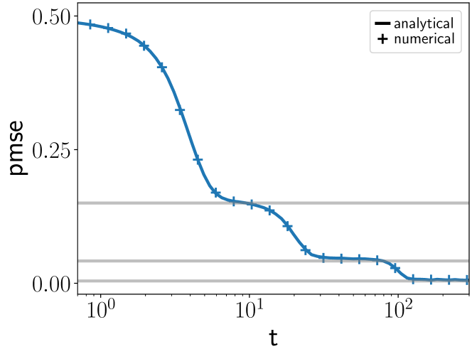
Figure 2: The dynamical equations describe the learning dynamics of autoencoders Prediction mean-squared error $\operatorname{\sf pmse}$ (2) of an autoencoder with $K\!=\!3$ hidden neurons during training on with stochastic gradient descent on the spiked Wishart model in the one-pass limit. We obtained the $\operatorname{\sf pmse}$ directly from a simulation (crosses) and from integration of the dynamical equations describing learning that we derive in section 3.1 (line). Horizontal lines indicate the PCA reconstruction error with increasing numbers of principal components. Parameters: $M\!=\!3,\eta\!=\!1$, $D\!=\!1000$.

3.1.3 Empirical verification

In fig. 2, we plot the $\operatorname{\sf pmse}$ of an autoencoder with $K\!=\!3$ hidden neurons during training on a dataset drawn from eq. 3 with $M\!=\!3$. We plot the $\operatorname{\sf pmse}$ both obtained from training the network using SGD (4) (crosses) and obtained from integrating the equations of motion that we just derived (lines). The agreement between the theoretical description in terms of bulk and spike modes captures the training dynamics well, even at an intermediate input dimension of $D\!=\!1000$. In the following, we analyse these equations, and hence the behaviour of the autoencoder during training, in more detail.

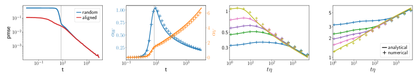
Figure 3: Two phases of learning in sigmoidal autoencoders. (a) Prediction error $\operatorname{\sf pmse}$ (2) of a sigmoidal autoencoder with a single hidden neuron starting from random initial conditions (blue). The error first decays exponentially, then as a power law. During this second phase of learning, the $\operatorname{\sf pmse}$ is identical to the $\operatorname{\sf pmse}$ of an autoencoder whose weights are proportional to the leading eigenvector $\Gamma$ of the input covariance at all times: $w(t)\propto\alpha_{w}(t)\Gamma,\quad v(t)\propto\alpha_{v}(t)\Gamma$, cf. eq. 19. (b) Dynamics of the scaling constants $\alpha_{w}$ and $\alpha_{v}$ obtained through simulations of an autoencoder starting from random weights (crosses) and from integration of a reduced set of dynamical equations, eq. C.8. (c,d) The norm of the encoder (left) and decoder (right) weights. Their weights shrink, respectively grow, as a power law $\sqrt{\rho}(\eta t)^{\pm\delta}$ with exponent $\delta\simeq 1/6$. This allows the sigmoidal network to remain in the linear region of its activation function and to achieve PCA performance. Solid lines are obtained from integration of a reduced set of dynamical equations, eq. C.8, crosses are from simulations for various combinations of learning rates and leading eigenvalue $\rho$ (different colours). Parameters: $D=500,\eta=1(a,b),M=1,K=1$.

3.2 Nonlinear autoencoders learn principal components sequentially

The dynamical equations of the encoder-encoder overlap $q^{k\ell}$, eq. B.28, takes the form

$$\frac{\partial q^{k\ell}_{1}(\rho,t)}{\partial t} =\frac{\eta\rho}{D}\left\{\cdots\right\}.$$ (15)

The learning rate of each mode of $q^{k\ell}$ is thus rescaled by the corresponding eigenvalue, suggesting that the principal components that correspond to each to each mode are learnt at different speeds, with the modes corresponding to the largest eigenvalues being learnt the fastest. For the other order parameters $r^{k\ell}$ and $t^{k\ell}$, all the terms in the equations of motion eq. B.24 and eq. B.29 are rescaled by $\rho$ except for one:

$$\frac{\partial r^{k\ell}_{1}(\rho,t)}{\partial t} =\frac{\eta\rho}{D}\left\{\cdots\right\}-\eta\sum_{a}r^{ak}(\rho,s)I^{\ell a}_{2}(Q_{1}),$$ (16)

$$\frac{\partial t^{k\ell}_{1}(\rho,t)}{\partial t} =\frac{\eta\rho}{D}\left\{\cdots\right\}-\eta\sum_{a}t^{\ell a}(\rho,s)I^{ka}_{2}(Q_{1})$$ (17)

Indeed, the $\operatorname{\sf pmse}$ of the sigmoidal autoencoder shown in fig. 2 goes through several sudden decreases, preceded by plateaus with quasi-stationary $\operatorname{\sf pmse}$. Each transition is related to the network “picking up” an additional principal component. By comparing the error of the network on the plateaus to the PCA reconstruction error with an increasing number of principal components (solid horizontal lines in fig. 2), we confirm that the plateaus correspond to stationary points where the network has learnt (a rotation of) the first leading principal components. Whether or not the plateaus are clearly visible in the curves depends on the separation between the eigenvalues of the leading eigenvectors.

This sequential learning of principal components has also been observed in several other models of learning. It appears in unsupervised learning rules such as Sanger’s rule (Sanger, 1989) (aka as generalised Hebbian learning, cf. appendix A) that was analysed by Biehl & Schlösser (1998). Gunasekar et al. (2017); Gidel et al. (2019) found a sudden transition from the initial to the final error in linear models $\hat{\boldsymbol{x}}=\text{{W}}\boldsymbol{x}$, but step-wise transitions for factorised models, i.e. linear autoencoders of the form $\hat{\boldsymbol{x}}=\text{{V}}\text{{W}}\boldsymbol{x}$. Saxe et al. (2019) also highlighted the sequential learning of principal components, sorted by singular values.

The evolution of the bulk order parameters obeys

$$\begin{split}\frac{\partial T^{kl}_{\text{bulk}}}{\partial s}&=-\eta\sum_{a}T^{al}_{\text{bulk}}\mathbb{E}\,g(\lambda^{k})g(\lambda^{a})+(k\leftrightarrow\ell)\\ \frac{\partial R^{kl}_{\text{bulk}}}{\partial s}&=-\eta\sum_{a}R^{al}_{\text{bulk}}\mathbb{E}\,g(\lambda^{k})g(\lambda^{a}),\quad\frac{\partial Q^{kl}_{\text{bulk}}}{\partial s}=0\end{split}$$ (18)

As a consequence, in the early stages of training, to first approximation, the bulk component of $\text{{R}}_{1}$ and $\text{{T}}_{1}$ follow an exponential decay towards $0$. The characteristic time of this decay is given by the expectation $\mathbb{E}\,g(\lambda^{k})g(\lambda^{\ell})|_{s=0}$ which only depends on $\text{{Q}}_{1}|_{s=0}$. In addition, the last equation implies that the evolution of $\text{{Q}}_{1}$ is entirely determined by the dynamics of the spike modes.

3.3 The long-time dynamics of learning: align, then rescale

At long training times, we expect a sigmoidal autoencoder with untied weights to have retrieved the leading PCA subspace since it achieves the PCA reconstruction error. This motivates an ansatz for the dynamical equations where the network weights are proportional to the eigenvectors of the covariance $\Gamma^{k}$,

$$w_{i}^{k}(t)=\nicefrac{{\alpha^{k}_{\omega}(t)}}{{\sqrt{D}}}\;\Gamma_{i}^{k}\qquad v_{i}^{k}=\alpha^{k}_{v}(t)\Gamma_{i}^{k},$$ (19)

where $\boldsymbol{\alpha}_{\omega},\boldsymbol{\alpha}_{v}\in\mathbb{R}^{K}$ are scaling constants that evolve in time. With this ansatz, the order parameters are diagonal, and we are left with a reduced set of $2K$ equations describing the dynamics of $\alpha_{w}^{k}$ and $\alpha^{k}_{v}$ which are given in eq. C.8 together with their detailed derivation.

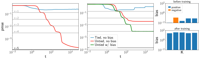
Figure 4: Shallow autoencoders require untied weights, and ReLU autoencoders also need biases. (a) Prediction error $\operatorname{\sf pmse}$ (2) of sigmoidal autoencoders with untied weights (red) and with tied weights $v^{k}=w^{k}$ (blue). Horizontal lines indicate PCA errors for rank $r$. (b) Same plot for ReLU autoencoders with three different architectures: tied weights, no bias (blue), untied weights without bias (red) and untied weights with bias (green). Only the latter architecture achieves close to PCA error. (c) Distribution of biases in a ReLU network before (top) and after training (bottom). The biases increase throughout training, hence pushing the network into the linear region of its activation function. Parameters: $D=1000,K=5,\eta=1$.

We first verify the validity of the reduced equations (C.8) to describe the long-time dynamics of sigmoidal autoencoders. In fig. 3(a), we show the generalisation dynamics of a sigmoidal autoencoder starting from random initial conditions (blue). We see two phases of learning: after an exponential decay of the $\operatorname{\sf pmse}$ up to time $t\sim 10$, the $\operatorname{\sf pmse}$ decays as a power-law. This latter decay is well captured by the evolution of the $\operatorname{\sf pmse}$ of a model which we initialised with weights aligned to the leading PCs. We deduce that during the exponential decay of the error, the weights align to the leading PCA directions and stay aligned during the power-law decay of the error.

After having recovered the suitable subspace, the network adjusts the norm of its weights to decrease the error. A look at the dynamics of the scale parameters $\boldsymbol{\alpha}_{w}$ and $\boldsymbol{\alpha}_{v}$ during this second phase of learning reveals that the encoder’s weights shrink, while the decoder’s weights grow, cf. fig. 3(b). Together, these changes lead to the power-law decay of the $\operatorname{\sf pmse}$. Note that we chose a dataset with only one leading eigenvalue so as to guarantee that the AE recovers the leading principal component, rather than a rotation of them. A scaling analysis of the evolution of the scaling constants $\alpha^{k}_{w}$ and $\alpha^{k}_{v}$ shows that the weights decay, respectively grow, as a power-law with time, $\alpha^{k}_{w}\propto\nicefrac{{1}}{{\sqrt{\rho}}}\;(\eta t)^{-\delta}$ and $\alpha^{k}_{v}\propto\nicefrac{{1}}{{\sqrt{\rho}}}\;(\eta t)^{\delta}$, see fig. 3(c-d).

We can understand this behaviour by recalling the linearity of $g(x)~{}\!=~{}\!\erf\left(\nicefrac{{x}}{{\sqrt{2}}}\right)$ around the origin, where $g(x)~{}\!\sim\!~{}\sqrt{\nicefrac{{2}}{{\pi}}}\;x$. By shrinking the encoder’s weights, the autoencoder thus performs a linear transformation of its inputs, despite the non-linearity. It recovers the linear performance of a network given by PCA if the decoder’s weights grow correspondingly for the reconstructed input $\hat{\boldsymbol{x}}$ to have the same norm as the input $\boldsymbol{x}$.

We can find a relation between the scaling constants $\alpha^{k}_{v}$ and $\alpha^{k}_{w}$ at long times using the ansatz eq. 19 in the expression of the $\operatorname{\sf pmse}$:

$$\begin{split}\operatorname{\sf pmse}=\sum_{k=1}^{K}\underbrace{\left\{\tilde{\rho}_{k}+\alpha_{v}^{k2}\mathbb{E}\,g(\lambda^{k})^{2}-2\mathbb{E}\,\nu^{k}g(\lambda^{k})\right\}}_{f(\alpha^{k}_{v},\alpha^{k}_{w})}+\sum_{k>K}^{D}\tilde{\rho}_{k},\end{split}$$ (20)

where the second term is simply the rank $K$ PCA error. The first term should be minimised to achieve PCA error, i.e. $f(\alpha^{k}_{w},\alpha_{v}^{k*})\!=\!0$ for all $k$. For a linear autoencoder, we find $\alpha_{v}^{k*}\!=\!\nicefrac{{1}}{{\alpha_{w}^{k}}}$: as expected, any rescaling of the encoder’s weights needs to be compensated in the decoder. For a sigmoidal autoencoder instead, we find

$$\alpha_{v}^{k*}= \frac{1}{\alpha_{w}^{k}}\sqrt{\frac{\pi}{2}\left(1+\tilde{\rho}^{k}\alpha_{w}^{k2}\right)}$$ (21)

Note, that at small $\alpha^{k}_{w}$ we recover the linear scaling $\alpha^{k*}_{v}~{}\!~{}\sim~{}\!~{}\left(g^{\prime}(0)\alpha^{k}_{w}\right)^{-1}$.

The importance of untying the weights for sigmoidal autoencoders

The need to let the encoder and decoder weights grow, resp. shrink, to achieve PCA error makes learning impossible in sigmoidal autoencoders with tied weights, where $\boldsymbol{v}^{k}\!=\!\boldsymbol{w}^{k}$. Such an autoencoder evidently cannot perform the rescaling required to enter the linear regime of its activation function, and is therefore not able able to achieve PCA error. Even worse, the learning dynamics shown in fig. 4(a) show that a sigmoidal autoencoder with tied weights (blue) hardly achieves a reconstruction error better than chance, in stark contrast to the same network with untied weights (red).

3.4 The importance of the bias in ReLU autoencoders

Sigmoidal autoencoders achieve the PCA error by exploiting the linear region of their activation function. We can hence expect that in order to successfully train a ReLU AE, which is linear for all positive arguments, it is necessary to add biases at the hidden layer. The error curves for ReLU autoencoders shown in fig. 4(b) show indeed that ReLU autoencoders achieve an error close to the PCA error only if the weights are untied and the biases are trained. If the biases are not trained, we found that a ReLU autoencoder with $K$ hidden neurons generally achieves a reconstruction error of roughly $K/2$, presumably because only $K/2$ nodes have a positive pre-activation and can exploit the linear region of ReLU. Training the biases consistently resulted in large, positive biases at the end of training, fig. 4(c). The large biases, however, result in a small residual error that negatively affects the final performance of a ReLU network when compared to the PCA performances, as can be seen from linearising the output of the ReLU autoencoder:

$$\hat{\boldsymbol{x}}=\sum_{k}\boldsymbol{v}^{k}\max(0,\lambda^{k}+b^{k})=\underbrace{\sum_{k}\boldsymbol{v}^{k}\lambda^{k}}_{\text{PCA}}+\underbrace{\sum_{k}\boldsymbol{v}^{k}b^{k}}_{\text{residual}},$$ (22)

where $b^{k}\in\mathbb{R}$ is the bias of the $k$th neuron.

3.5 Breaking the symmetry of SGD yields the exact principal components

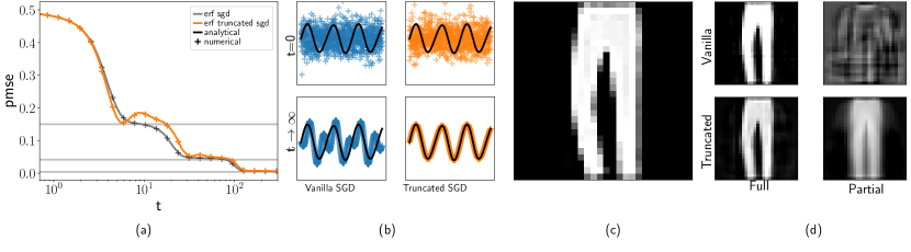
Figure 5: Breaking the symmetry between neurons yields the exact principal components of the data. (a) Prediction mean-squared error (2) of an autoencoder trained using vanilla SGD (eq. 4, blue) and truncated SGD (eq. 23, orange). Grey horizontal lines indicate PCA reconstruction errors. (b) We show the weight vector of the first neuron of the autoencoder before and after training (top vs bottom) with vanilla and truncated SGD (left and right, resp.). In contrast to vanilla SGD, truncated SGD recovers the true leading principal component of the inputs, a sinusoidal wave (black). (c) Example image taken from Fashion MNIST. (d) The left column shows reconstructions of the image from (c) using all $K=64$ neurons of an autoencoder trained with vanilla (top) and truncated SGD (bottom) on the full Fashion MNIST database. The right column shows reconstructions using only the first 5 neurons of the same autoencoders. Parameters: $\eta=1$, $K=4$ ((a) and (b)), $K=64$ ((c) and (d)), $bs=1,P=60000$.

Linear autoencoders do not retrieve the exact principal components of the inputs, but some rotation of them due to the rotational symmetry of the square loss (Bishop, 2006). While this does not affect performance, it would still be desirable to obtain the leading eigenvectors exactly to identify the important features in the data.

The symmetry between neurons can be broken in a number of ways. In linear autoencoders, previous work considered applying different amounts of regularisation to each neuron (Mianjy et al., 2018; Plaut, 2018; Kunin et al., 2019; Bao et al., 2020) or optimising a modified loss (Oftadeh et al., 2020). In unsupervised learning, Sanger’s rule (Sanger, 1989) breaks the symmetry by making the update of the weights of the first neuron independent of all other neurons; the update of the second neuron only depends on the first neuron, etc. This idea was extended to linear autoencoders by Oftadeh et al. (2020); Bao et al. (2020). We can easily extend this approach to non-linear autoencoders by training the decoder weights following

$$\differential v_{i}^{k}=-\frac{\eta_{V}}{D}g(\lambda^{k})\left(x_{i}-\sum_{\ell=1}^{{\color[rgb]{1,0,0}k}}v^{\ell}_{i}g(\lambda^{\ell})\right),$$ (23)

where the sum now only runs up to $k$ instead of $K$. The update for the encoder weights $\boldsymbol{w}^{k}$ is unchanged from eq. 4, but the error term is changed to $\Delta_{i}^{k}\!=\!x_{i}-\sum_{\ell=1}^{{\color[rgb]{1,0,0}k}}v^{\ell}_{i}g(\lambda^{\ell})$.

We can appreciate the effect of this change by considering a fixed point $\{\text{{W}}^{*},\text{{V}}^{*}\}$ of the vanilla SGD updates eq. 4 with $\differential\boldsymbol{w}^{*k}\!=\!0$ and $\differential\boldsymbol{v}^{*k}\!=\!0$. Multiplying this solution by an orthogonal matrix $\text{{O}}\!\in\!O(K)$ i.e. $\{\tilde{\text{{W}}},\tilde{\text{{V}}}\}\!=\!\{\text{{O}}\text{{W}}^{*},\text{{O}}\text{{V}}^{*}\}$ yields another fixed point, since

$$\begin{split}\differential\tilde{v}^{k}_{i}&=-\frac{\eta_{V}}{D}g(\tilde{\lambda}^{k})\left(x_{i}-\sum_{\ell_{1}\ell_{2}=1}^{K}\underbrace{\sum_{\ell=1}^{K}O^{\ell\ell_{2}}O^{\ell\ell_{3}}}_{\delta^{\ell_{2}\ell_{3}}}v^{*\ell_{2}}_{i}g(\lambda^{*\ell_{3}})\right)\\ &=-\frac{\eta_{V}}{D}g(\tilde{\lambda}^{k})\left(x_{i}-\sum_{\ell=1}^{K}v^{*\ell}_{i}g(\lambda^{*\ell})\right)=0\end{split}$$ (24)

for the decoder, and likewise for the encoder weights. For truncated SGD (23), the underbrace term in eq. 24 is no longer the identity and the rotated weights $\{\tilde{\text{{W}}},\tilde{\text{{V}}}\}$ are no longer a fixed point.

We show the $\operatorname{\sf pmse}$ of a sigmoidal autoencoder trained with vanilla and truncated SGD in fig. 5(a), together with the theoretical prediction from a modified set of dynamical equations. The theory captures both learning curves perfectly, and we can see that using truncated SGD incurs no performance penalty - both autoencoders achieve the PCA reconstruction error. Note that the reconstruction error can increase temporarily while training with the truncated algorithm since the updates do not minimise the square loss directly. In this experiment, we trained the networks on a synthetic dataset where the eigenvectors are chosen to be sinusoidal (black lines in fig. 5 b). As desired, the weights of the network trained with truncated SGD converges to the exact principal components, while vanilla SGD only recovers a linear combination of them.

The advantage of recovering the exact principal components is illustrated with the partial reconstructions of a test image from the FashionMNIST database (Xiao et al., 2017). We train autoencoders with $K\!=\!64$ neurons to reconstruct FashionMNIST images using the vanilla and truncated SGD algorithms until convergence. We show the reconstruction using all the neurons of the networks in the left column of fig. 5(d). Since the networks achieve essentially the same performance, both reconstructions look similar. The partial reconstruction using only the first five neurons of the networks shown on the right are very different: while the partial reconstruction from truncated SGD is close to the original image, the reconstruction of the vanilla autoencoder shows traces of pants mixed with those of a sweatshirt.

4 Representation learning on realistic data under standard conditions

We have derived a series of results on the training of non-linear AEs derived in the case of synthetic, Gaussian datasets. Most of our simplifying assumptions are not valid on real datasets, because they contain only a finite number of samples, and because these samples are finite-dimensional and not normally distributed. Furthermore, we had to choose certain scalings of the pre-activations (5) and the learning rates to ensure the existence of a well-defined asymptotic limit $D\to\infty$. Here, we show that the dynamical equations of section 3.1 describe the dynamics of an autoencoder trained on more realistic images rather well, even if we don’t perform any explicit rescalings in the simulations.

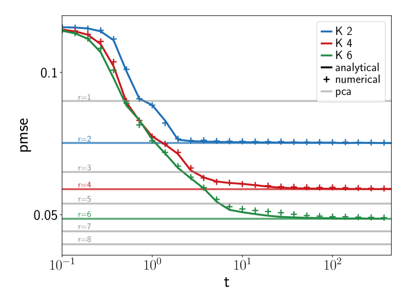
Figure 6: Theory vs. simulations for sigmoidal autoencoders trained on CIFAR10. Prediction mean-squared error $\operatorname{\sf pmse}$ (2) of a sigmoidal autoencoder with $K=2,4,6$ hidden neurons trained on 10 000 greyscale CIFAR10 images (Krizhevsky et al., 2009) (crosses). Solid lines show the $\operatorname{\sf pmse}$ predicted from integrating the dynamical equations of section 3.1, using the empirical covariance matrix of the training inputs. Horizontal lines indicate the PCA error with varying rank $r$. Parameters: $D=1024,\eta=1$.

Realistic data

In fig. 6, we show the $\operatorname{\sf pmse}$ of autoencoders of increasing size trained on 10k greyscale images from CIFAR10 (Krizhevsky et al., 2009) with crosses. The solid lines are obtained from integration the equations of motion of appendix B, using the empirical covariance of the training images. The accuracy of the equations to describe the learning dynamics at all times implies that the low-dimensional projections $\boldsymbol{\lambda}$ and $\boldsymbol{\nu}$ introduced in eq. 5 are very close to being normally distributed. This is by no means obvious, since the images clearly do not follow a normal distribution and the weights of the autoencoder are obtained from training on said images, making them correlated with the data. Instead, fig. 6 suggests that from the point of view of a shallow, sigmoidal autoencoder, the inputs can be replaced by Gaussian vectors with the same mean and covariance without changing the dynamics of the autoencoder. In fig. 8 in the appendix, we show that this behaviour persists also for ReLU autoencoders and, as would be expected, for linear autoencoders. Nguyen (2021) observed a similar phenomenon for tied-weight autoencoders with a number of hidden neurons that grows polynomially with the input dimension $D$. We also verified that several insights developed in the case of Gaussian data carry over to real data. In particular, we demonstrate in fig. 9 that sigmoidal AE require untied weights to learn, ReLU networks require adding biases to the encoder weights, and that the principal components of realistic data are also learnt sequentially.

Relation to the Gaussian equivalence

The fact that the learning dynamics of the autoencoders trained on CIFAR10 are well captured by an equivalent Gaussian model is an example of the Gaussian equivalence principle, or Gaussian universality, that received a lot of attention recently in the context of supervised learning with random features (Liao & Couillet, 2018; Seddik et al., 2019; Mei & Montanari, 2021) or one- and two-layer neural networks (Hu & Lu, 2020; Goldt et al., 2020, 2022; Loureiro et al., 2021). These works showed that the performance of these different neural networks is asymptotically well captured by an appropriately chosen Gaussian model for the data. While previous work on Gaussian equivalence in two-layer networks crucially assumes that the network has a number of hidden neurons $K$ that is small compared to the input dimension, here we find that the Gaussian equivalence of autoencoders extends to essentially any number of hidden neurons, for example $K=D/2$, as we show in fig. 8 in the appendix.

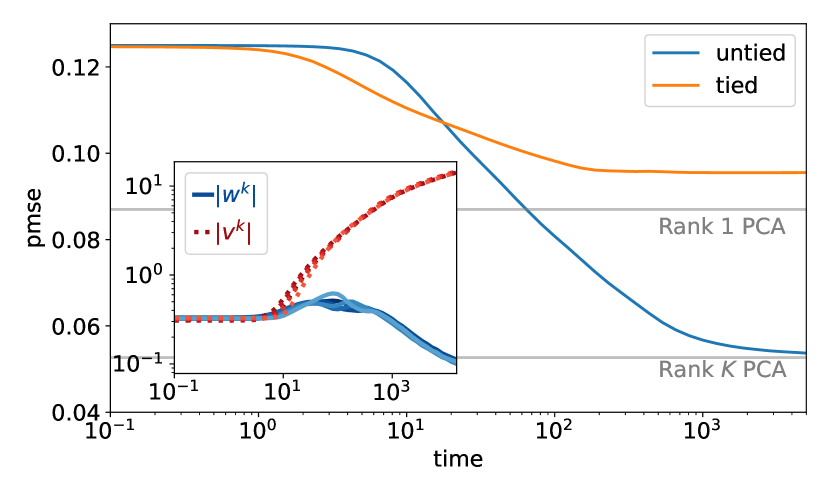
Figure 7: Training an autoencoder without explicit rescalings Prediction mean-squared error (pmse) of a sigmoidal autoencoder (AE) on grayscale CIFAR10 using vanilla SGD with untied (blue) and tied (orange) weights. In this experiment, we did not rescale the eigenvalues of the data, the pre-activations (5), or the learning rates. Inset: $\ell_{2}$ norm of decoder (blue) and encoder (red) weights. Parameters: $D=1024,K=5,\eta=10^{-2}$

Robustness of the dynamical equations to rescalings

The scaling of the local fields in eq. 5, and hence of the order parameters, is necessary to ensure that in the high-dimensional limit $D\to\infty$, all three terms in the $\operatorname{\sf pmse}$ are non-vanishing. As we describe in the derivation, the rescaling of the learning rates are then necessary to obtain a set of closed equations. Nevertheless, we verified that the conclusions of the paper are not an artefact of these scalings. To this end, we trained a sigmoidal AE $\hat{x}_{i}=\sum_{k}^{K}v^{k}_{i}g(w^{k}x)$ on grayscale CIFAR10 using SGD without rescaling the eigenvalues of the inputs, pre-activations $\lambda^{k}=w^{k}x$, or the learning rates. As we show in fig. 7, we recover the three key phenomena described in the paper: autoencoders with tied weights fail to achieve rank-1 PCA error (orange); autoencoders with untied weights achieve rank-$K$ PCA error (blue); and for sigmoidal autoencoders, the encoder weights $w$ shrink, while decoder weights $v$ grow to reach the linear regime (inset). These results underline that our theoretical results describe AEs under “standard conditions”.

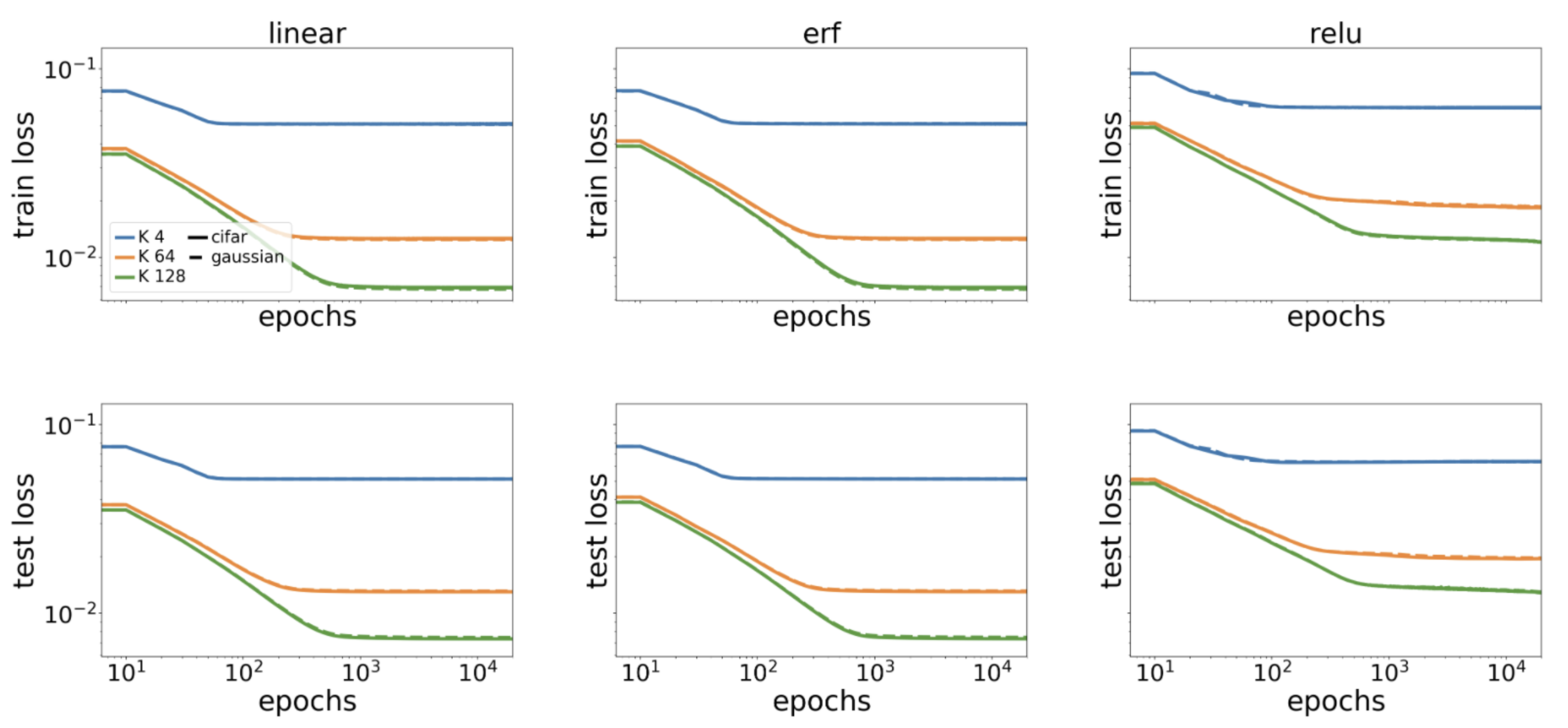
Figure 8: Gaussian equivalence for autoencoders Train and test mean-squared error for linear, sigmoidal and relu autoencoders with different numbers of hidden neurons ($K=4,64,128$ in blue, orange and green, resp.) The autoencoders were trained on CIFAR10 grayscale images (solid lines) or, starting from the same initial conditions, on Gaussian inputs with the same covariance (dashed lines). The agreement is essentially perfect. Parameters: 10k training samples, $D=1024$, mini-batch size=1, $\eta=1$.

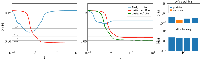
Figure 9: Results derived on synthetic data carry over to finite real datasets (a) Also in real dataset, a sigmoidal AE requires untied weights to attain good performances. For an untied student, which asymptotically performs as PCA, the dynamics slow down at intermediary ranks, signalling a sequential learning of different modes. (b) In order to learn, a ReLU autoencoder requires training the bias in the encoder’s weights. The asymptotic error is given by PCA plus a residual due to the biases. Parameters: CIFAR10 and FashionMNIST with 10k images. batch-size=1, $\eta=1$.

Appendix A Online learning algorithms for PCA

We briefly review a number of unsupervised learning algorithms for principal component analysis, leading to Sanger’s rule which is the inspiration for the truncated SGD algorithm of section 3.5.

Setup

We consider inputs $\boldsymbol{x}=(x_{i}),i=1,\ldots,D$ with first two moments equal to

$$\mathbb{E}\,x_{i}=0\mbox{\quad and\quad}\mathbb{E}\,x_{i}x_{j}=\Omega_{ij}.$$ (A.1)

We work in the thermodynamic limit $D\to\infty$.

Hebbian learning

The Hebbian learning rule allows to obtain an estimate of the leading PC by considering a linear linear model $y=\lambda=\sum_{i}\nicefrac{{w_{i}x_{i}}}{{\sqrt{D}}}$ with $i=1,\ldots,D$ and the loss function $\mathcal{L}(\lambda)=-\lambda^{2}$. It updates the weights as:

$$\differential w_{i}^{t}=-\eta_{t}\nabla_{w_{i}}\mathcal{L}(\lambda)=\frac{1}{\sqrt{D}}\eta_{t}yx_{i}$$ (A.2)

In other words, the Hebbian learning rule tries to maximise the second moment of the pre-activation $\lambda$. That using this update we obtain an estimate of the first principal component makes intuitive sense. Consider the average over the inputs of the loss:

$$\mathbb{E}\,\mathcal{L}(\lambda)=-\frac{1}{D}w_{i}\Omega_{ij}w_{j}.$$ (A.3)

If the weight vector $\boldsymbol{w}$ is equal to the $\tau$th eigenvector of $\Omega$, then $\mathbb{E}\,\mathcal{L}(\lambda)=-\rho_{\tau}/D$, and the loss is minimised by converging to the eigenvector with the larges eigenvalue. Also note, that similar to what we find in the main text, this result also suggests that the leading eigenvalue in the large-$D$ limit should scale as $\rho_{\tau}\sim D$. The Hebbian rule has the well-known deficit that it imposes no bound on the growth of the weight vector. A natural remedy is to introduce some form of weight decay such that

$$\differential w_{i}^{t}=\frac{\eta}{\sqrt{D}}(yx_{i}-\kappa w_{i}).$$ (A.4)

Oja’s rule (Oja, 1982) offers a smart choice for the weight decay constant $\kappa$. Consider the same linear model $y=\lambda$ trained with a Hebbian rule and weight decay $\kappa=y^{2}$:

$$\differential w_{i}^{t}=\frac{\eta}{\sqrt{D}}(yx_{i}-y^{2}w_{i})$$ (A.5)

The purpose of this choice can be appreciated from substituting in the linear model and setting the update rule to zero, which yields (dropping the constants)

$$\sum_{j}\Omega_{ij}w_{j}=\sum_{j,l}w_{j}\Omega_{j\ell}w_{\ell}w_{i}$$ (A.6)

which is precisely the eigenvalue equation for $\Omega$.

Then, Oja’s update rule is then derived from Hebb’s rule by adding normalisation to the Hebbian update (A.2),

$$w_{i}^{t+1}=\frac{w_{i}^{t}+\eta yx_{i}}{\left(\sum\left[w_{i}^{t}+\eta yx_{i}\right]^{p}\right)^{1/p}}$$ (A.7)

with $p$ integer (in Oja’s original paper, $p=2$.) This learning rule can be seen as a power iteration update. Substituting for $y$, we see that the numerator corresponds to, on average, repeated multiplication of the weight vector with the average covariance matrix. Expanding eq. A.7 around $\eta=0$ yields Oja’s algorithm (while also assuming that the weight vector is normalised to one). One can show that Oja’s rule indeed converges to the PC with the largest eigenvalue by allowing the learning rate to vary with time and imposing the mild conditions

$$\lim_{T\to\infty}\sum_{t=0}^{T}\eta_{t}\to\infty,\qquad\qquad\lim_{T\to\infty}\sum_{t=0}^{T}\eta_{t}^{p}<\infty\mbox{\quad for\quad}p>1.$$ (A.8)

Sanger’s rule (Sanger, 1989)

is also known as generalised Hebbian learning in the literature and extends the idea behind Oja’s rule to networks with multiple outputs $y^{k}=w^{k}_{i}x_{i}$. It allows estimation of the first few leading eigenvectors by using the update rule is given by

$$\differential w^{k}_{i}=\frac{\eta}{\sqrt{D}}y^{k}\left(x_{i}-\sum_{\ell=1}^{k}y^{\ell}w^{\ell}_{i}\right).$$ (A.9)

Note that the second sum extends only to the $k$; the dynamics of the $k$th input vector hence only depends on weight vectors $w^{\ell}$ with $\ell<k$. This dependence is one of the similarities of Sanger’s rule with the Gram-Schmidt procedure for orthogonalising a set of vectors (cf. sec. 0.6.4 of Horn & Johnson (2012)). The dynamics of Sanger’s rule in the online setting were studied by Biehl & Schlösser (1998); Schlösser et al. (1999). Sanger’s rule reduces to Oja’s rule for $K=1$.

Appendix B Online learning in autoencoders

Here we derive the set of equations tracking the dynamics of shallow non-linear autoencoders trained in the one-pass limit of stochastic gradient descent (SGD). These equations are derived for Gaussian inputs $\boldsymbol{x}\in\mathbb{R}^{D}$ drawn from the generative model eq. 3, but as we discuss in section 4, they also capture accurately the dynamics of training on real data.

B.1 Statics

The starting point of the analysis is the definition of the test error (2) and the identification of order parameters, i.e. low dimensional overlaps of high dimensional vectors.

$$\operatorname{\sf pmse} \equiv\frac{1}{D}\sum_{i}\mathbb{E}(x_{i}-\hat{x}_{i})^{2}$$ (B.1)

$$=\frac{1}{D}\Tr\boldsymbol{\Omega}+\frac{1}{D}\sum_{i}\sum_{k,\ell}v_{i}^{k}v_{i}^{\ell}\mathbb{E}\,g\left(\sum_{i}\frac{w^{k}_{i}x_{i}}{\sqrt{D}}\right)g\left(\sum_{i}\frac{w^{\ell}_{i}x_{i}}{\sqrt{D}}\right)-2\frac{1}{D}\sum_{i}\sum_{k}v^{k}_{i}x_{i}g\left(\sum_{i}\frac{w^{k}_{i}x_{i}}{\sqrt{D}}\right).$$ (B.2)

First we introduce the local fields corresponding to the encoder and decoder’s weights,

$$\lambda^{k}\equiv\sum_{i}\frac{w^{k}_{i}x_{i}}{\sqrt{D}}\qquad\nu^{k}\equiv\sum_{i}\frac{v^{k}_{i}x_{i}}{D},$$ (B.3)

as well as the order parameter tracking the overlap between the decoder weights:

$$T^{k\ell}_{0}\equiv\frac{1}{D}\sum_{i}v^{k}_{i}v^{\ell}_{i}.$$ (B.4)

Note the unusual scaling of $\nu^{k}$ with $D$; the intuition here is that in shallow autoencoders, the second-layer weights will be strongly correlated with the eigenvectors of the input-input covariance, and hence with the inputs, requiring the scaling $1/D$ instead of $1/\sqrt{D}$. This scaling is also the one that yields a set of self-consistent equations in the limit $D\to\infty$. The generalisation error becomes

$$\operatorname{\sf pmse}=\frac{1}{D}\Tr\Omega+\sum_{k,\ell}T_{0}^{k\ell}\mathbb{E}\,g(\lambda^{k})g(\lambda^{\ell})-2\sum_{k}\mathbb{E}\,\nu^{k}g(\lambda^{k}).$$ (B.5)

Crucially, the local fields $\lambda$ and $\nu$ are jointly Gaussian since the inputs are Gaussian. Since we have $\mathbb{E}\,\lambda^{k}=\mathbb{E}\,\nu^{k}=0$, the $\operatorname{\sf pmse}$ can be written in terms of the second moments of these fields only:

$$T_{1}^{k\ell}\equiv\mathbb{E}\,\nu^{k}\nu^{\ell}=\frac{1}{D^{2}}\sum_{i,j}v^{k}_{i}\Omega_{ij}v^{\ell}_{j},$$ (B.6)

$$Q_{1}^{k\ell}\equiv\mathbb{E}\,\lambda^{k}\lambda^{\ell}=\frac{1}{\sqrt{D}}\sum_{i,j}w^{k}_{i}\Omega_{ij}w^{\ell}_{j},$$ (B.7)

$$R_{1}^{k\ell}\equiv\mathbb{E}\,\nu^{k}\lambda^{\ell}=\frac{1}{D^{\nicefrac{{3}}{{2}}}}\sum_{i,j}v^{k}_{i}\Omega_{ij}w^{\ell}_{j}.$$ (B.8)

The full expression of $\mathbb{E}\,g(\lambda^{k})g(\lambda^{\ell})$ and $\mathbb{E}\,\nu^{k}g(\lambda^{k})$ in terms of the order parameters is given, for various activation functions, in App D. Note the different scalings of these overlaps with $D$. These are a direct consequence of the different scaling of the local fields $\lambda^{k}$ and $\nu^{k}$. In order to derive the equations of motion, it is useful to introduce the decomposition of $\boldsymbol{\Omega}$ in its eigenbasis:

$$\Omega_{rs}=\frac{1}{D}\sum_{\tau=1}^{D}\Gamma_{s\tau}\Gamma_{r\tau}\rho_{\tau}.$$ (B.9)

The eigenvectors $\Gamma_{s\tau}$ are normalised as $\sum_{i}\Gamma_{\tau i}\Gamma_{\tau^{\prime}i}=D\delta_{\tau\tau^{\prime}}$ and $\sum_{\tau}\Gamma_{\tau i}\Gamma_{\tau j}=D\delta_{ij}$. We further define the rotation of any $z_{i}\in\{w^{k}_{i},v^{k}_{i},x_{i}\}$ onto this basis as $z_{\tau}\equiv\nicefrac{{1}}{{\sqrt{D}}}\sum_{s=1}^{D}\Gamma_{\tau s}z_{s}$. The order parameters are then written:

$$T_{1}^{k\ell}=\frac{1}{D^{2}}\sum_{\tau}\rho_{\tau}v_{\tau}^{k}v_{\tau}^{\ell},\qquad R_{1}^{k\ell}=\frac{1}{D^{3/2}}\sum_{\tau}\rho_{\tau}w^{k}_{\tau}v^{\ell}_{\tau},\qquad Q_{1}^{k\ell}=\frac{1}{D}\sum_{\tau}\rho_{\tau}w^{k}_{\tau}w^{\ell}_{\tau}.$$ (B.10)

B.2 Averages over non-linear functions of weakly correlated variables

We briefly recall expressions to compute averages over non-linear functions of weakly correlated random variables that were also used by Goldt et al. (2020). These expressions will be extensively used in the following derivation. Consider $x$, $y\in\mathbb{R}$, two weakly correlated jointly Gaussian random variables with covariance matrix

$$M_{12}=\begin{bmatrix}C_{x}&\quad\epsilon M_{12}\\ \epsilon M_{12}&\quad C_{y}\end{bmatrix}$$ (B.11)

with $\epsilon\ll 1\in\mathbb{R}$ which encodes the weak correlation between $x$ and $y$. Then, the expectation of the product of any two real valued functions $f,h:\mathbb{R}\to\mathbb{R}$, is given, to leading order in $\epsilon$ by:

$$\mathop{\mathbb{E}\,}_{(x,y)}\left[f(x)h(y)\right]= \mathop{\mathbb{E}\,}_{x}\left[f(x)\right]\mathop{\mathbb{E}\,}_{y}\left[h(y)\right]$$

$$+\epsilon\mathop{\mathbb{E}\,}_{x}\left[f(x)(x-\bar{x})\right]\left(C_{x}^{-1}M_{12}C_{y}^{-1}\right)\mathop{\mathbb{E}\,}_{y}\left[h(y)(y-\bar{y})\right]+O(\epsilon^{2}).$$ (B.12)

Similarly, for 3 random variables $\{x_{i}\}$ with $x_{1}$ and $x_{2}$ weakly correlated with $x_{3}$ but not between each other, i.e. $\operatorname{Cov}(x_{1},x_{2})=M_{12}\!\sim\!O(1)$, one can compute the expectation of product of three real valued functions $f,g,h$ to leading order in $\epsilon$ as:

$$\begin{split}\mathbb{E}\,\left[f(x_{1})g(x_{2})h(x_{3})\right]=&\mathbb{E}\,\left[f(x_{1})g(x_{2})\right]\mathbb{E}\,\left[h(x_{3})\right]\\ &+\epsilon\frac{\mathbb{E}\,\left[h(x_{3})(x_{3}-\bar{x}_{3})\right]}{\left(C_{x_{1}}C_{x_{2}}-M_{12}^{2}\right)C_{x_{3}}}\left\{\mathbb{E}\,\left[f(x_{1})g(x_{2})(x_{1}-\bar{x}_{1})\right]M_{13}C_{x_{2}}\right.\\ &\hskip 110.00017pt\left.+\mathbb{E}\,\left[f(x_{1})g(x_{2})(x_{2}-\bar{x}_{2})\right]M_{23}C_{x_{1}}\right.\\ &\hskip 110.00017pt\left.-\mathbb{E}\,\left[f(x_{1})g(x_{2})(x_{1}-\bar{x}_{1})\right]M_{12}M_{23}\right.\\ &\hskip 110.00017pt\left.-\mathbb{E}\,\left[f(x_{1})g(x_{2})(x_{2}-\bar{x}_{2})\right]M_{13}M_{12}\right\}+O(\epsilon^{2}).\end{split}$$ (B.13)

B.3 Derivation of dynamical equations

At the $\mu$th step of training, the SGD update for the rotated weights reads

$$\differential w_{\tau}^{k}\equiv\left(w_{\tau}^{k}\right)_{\mu+1}-\left(w_{\tau}^{k}\right)_{\mu} =-\frac{\eta_{W}}{D}\frac{1}{\sqrt{D}}\sum_{j}^{D}\left(\sum_{\ell}^{K}v^{\ell}_{j}g(\lambda^{\ell})-x_{j}\right)v_{j}^{k}g^{\prime}(\lambda^{k})x_{\tau}-\frac{\kappa}{D}w_{\tau}^{k}$$

$$=-\frac{\eta_{W}}{\sqrt{D}}\left(\sum_{\ell}^{K}T_{0}^{\ell k}g(\lambda^{\ell})-\nu^{k}\right)g^{\prime}(\lambda^{k})x_{\tau}-\frac{\kappa}{D}w_{\tau}^{k},$$ (B.14)

$$\differential v_{\tau}^{k} =-\frac{\eta_{V}}{D}g(\lambda^{k})\left(\sum_{m}^{K}v_{\tau}^{m}g(\lambda^{m})-x_{\tau}\right)-\frac{\kappa}{D}v_{\tau}^{k}.$$ (B.15)

To keep notation concise, we drop the weight decay term in the following analysis. We can now compute the update of the various order parameters by inserting the above into the definition of the order parameters. The stochastic process described by the resulting equations concentrates, in the $D\to\infty$ limit, to its expectation over the input distribution. By performing the average over a fresh sample $x$, we therefore obtain a closed set of deterministic ODEs tracking the dynamics of training in the high-dimensional limit. We also show in simulations that these are able to capture well the dynamics also at finite dimension $D\sim 500$.

Update of $\text{{T}}_{0}$ the overlap of the decoder’s weights

Let us start with the update equation for $T_{0}^{k\ell}~{}=~{}\nicefrac{{1}}{{D}}\sum_{\tau}v_{\tau}^{k}v_{\tau}^{\ell}$ which is easily obtained by using the sgd update (B.3).

$$\begin{split}T_{0\mu+1}^{k\ell}-T_{0\mu}^{k\ell}=\frac{1}{D}\sum_{\tau}dv_{\tau}^{k}v_{\tau}^{\ell}+v_{\tau}^{k}dv_{\tau}^{\ell}=-\frac{\eta_{V}}{D}\left(\sum_{a}g(\lambda^{k})g(\lambda^{a})T_{0}^{a\ell}+\nu^{\ell}g(\lambda^{k})\right)+(k\leftrightarrow\ell)\end{split}$$ (B.16)

By taking the expectation over a fresh sample $x$ and the $D\to\infty$ limit of one-pass SGD, we obtain a continuous in the normalised number of steps $s=\nicefrac{{\mu}}{{D}}$, which we interpret as a continuous time variable, as:

$$\begin{split}\frac{\partial T_{0}^{k\ell}}{\partial s}=-\eta_{V}\left(\sum_{a}\mathbb{E}\,g(\lambda^{k})g(\lambda^{a})T_{0}^{a\ell}+\mathbb{E}\,\nu^{\ell}g(\lambda^{k})\right)+(k\leftrightarrow\ell),\end{split}$$ (B.17)

where the notation $(k\leftrightarrow\ell)$ indicates an additional term identical to the first except for exchange of the indices $k$ and $l$. This equation requires to evaluate $I_{22}\equiv\mathbb{E}\,g(\lambda^{k})g(\lambda^{k})$, $I_{21}\equiv\mathbb{E}\,\nu^{\ell}g(\lambda^{k})$, which are two-dimensional Gaussian integrals with covariance matrix given by the order parameters. We give their expression in appendix D. We also note that the second order term $\propto\differential v^{k}\differential v^{\ell}$ is sub-leading in the high dimensional limit we work in.

Update of $\text{{T}}_{1}$

The update equation for $T_{1}^{k\ell}~{}=~{}\nicefrac{{1}}{{D^{2}}}\sum_{\tau}\rho_{\tau}v_{\tau}^{k}v_{\tau}^{\ell}$ is obtained similarly as before by using the SGD update (B.3) and taking the high-dimensional limit.

$$\begin{split}\frac{\partial T_{1}^{k\ell}}{\partial s}=-\eta_{V}\left(\sum_{a}\mathbb{E}\,g(\lambda^{k})g(\lambda^{a})T_{1}^{al}+\sum_{\tau}\rho_{\tau}\frac{v^{\ell}_{\tau}}{D^{2}}\mathbb{E}\,g(\lambda^{k})x_{\tau}\right)+(k\leftrightarrow\ell)\end{split}$$ (B.18)

To make progress, we have to evaluate $\mathbb{E}\,g(\lambda^{k})x_{\tau}$. For this purpose it is crucial to notice that the rotated inputs $x_{\tau}$ are weakly correlated with the local fields:

$$\begin{split}\mathbb{E}\,\lambda^{k}x_{\tau}=\frac{1}{D}\sum_{i,j}w_{i}^{k}\Omega_{ij}\Gamma_{\tau j}=\frac{1}{\sqrt{D}}\rho_{\tau}w_{\tau}^{k},\\ \mathbb{E}\,\nu^{k}x_{\tau}=\frac{1}{D^{\nicefrac{{3}}{{2}}}}\sum_{i,j}v_{i}^{k}\Omega_{ij}\Gamma_{\tau j}=\frac{1}{D}\rho_{\tau}v_{\tau}^{k}.\end{split}$$ (B.19)

Then, we can compute the expectation $\mathbb{E}\,g(\lambda^{k})x_{\tau}$ using the results of section B.2, i.e. Eq. (B.2) with $f(x)=g(x)$ and $h(y)=y$, thus obtaining:

$$\mathbb{E}\,g(\lambda^{k})x_{\tau}=\frac{\mathbb{E}\,\lambda^{k}g(\lambda^{k})}{Q_{1}^{kk}}\frac{\rho_{\tau}w^{k}_{\tau}}{\sqrt{D}}$$ (B.20)

Inserting the above expression in the update of $\text{{T}}_{1}$ yields:

$$\frac{\partial T_{1}^{k\ell}}{\partial s} =\eta_{V}\left(\frac{\mathbb{E}\,\lambda^{k}g(\lambda^{k})}{Q_{1}^{kk}}\sum_{\tau}\rho^{2}_{\tau}\frac{v_{\tau}^{\ell}w^{k}_{\tau}}{D^{5/2}}-\sum_{a}\mathbb{E}\,g(\lambda^{k})g(\lambda^{a})T_{1}^{al}\right)+(k\leftrightarrow\ell)$$ (B.21)

Notice, that in this equation we have the the appearance of $\sum_{\tau}\rho^{2}_{\tau}\frac{v_{\tau}^{\ell}w^{k}_{\tau}}{D^{5/2}}$, a term which cannot be simply expressed in terms of order parameters. Similar terms appear in the equation for $\text{{Q}}_{1}$ and $\text{{R}}_{1}$. To close the equations, we are thus led to introduce order parameter densities in the next step.

Order parameters as integrals over densities

To proceed, we introduce the densities $q(\rho,s),r(\rho,s)$ and $t(\rho,s)$. These depend on $\rho$ and on the normalised number of steps $s=\nicefrac{{\mu}}{{D}}$:

$$\begin{split}q^{k\ell}(\rho,s)&=\frac{1}{D\epsilon_{\rho}}\sum_{\tau}w^{k}_{\tau}w^{\ell}_{\tau}\mathbbm{1}_{\left(\rho_{\tau}\in\mathopen{[}\rho,\rho+\varepsilon_{\rho}\mathclose{[}\right)},\\ r^{k\ell}(\rho,s)&=\frac{1}{D^{\nicefrac{{3}}{{2}}}\epsilon_{\rho}}\sum_{\tau}v^{k}_{\tau}w^{\ell}_{\tau}\mathbbm{1}_{\left(\rho_{\tau}\in\mathopen{[}\rho,\rho+\varepsilon_{\rho}\mathclose{[}\right)},\\ t^{k\ell}(\rho,s)&=\frac{1}{D^{2}\epsilon_{\rho}}\sum_{\tau}v^{k}_{\tau}v^{\ell}_{\tau}\mathbbm{1}_{\left(\rho_{\tau}\in\mathopen{[}\rho,\rho+\varepsilon_{\rho}\mathclose{[}\right)},\end{split}$$ (B.22)

where $\mathbbm{1}(.)$ is the indicator function and the limit $\epsilon_{\rho}\to 0$ is taken after the thermodynamic limit. The order parameters are obtained by integrating these densities over the spectrum of the input-input covariance matrix:

$$Q_{1}^{k\ell}=\frac{1}{D}\int\differential\rho p_{\Omega}(\rho)\rho q^{k\ell}(\rho,s),\quad R_{1}^{k\ell}=\frac{1}{D}\int\differential\rho p_{\Omega}(\rho)\rho r^{k\ell}(\rho,s),\quad T_{1}^{k\ell}=\frac{1}{D}\int\differential\rho p_{\Omega}(\rho)\rho t^{k\ell}(\rho,s).$$ (B.23)

It follows that tracking the dynamics of the functions $q,r$ and $t$, we obtain the dynamics of the overlaps $\text{{Q}}_{1},\text{{R}}_{1}$ and $\text{{T}}_{1}$.

Dynamics of $t(s,\rho)$

The dynamics of $t$ is given straightforwardly from eq. B.21 as:

$$\frac{\partial t^{k\ell}(\rho,s)}{\partial s} =\eta_{V}\left(\frac{\mathbb{E}\,\lambda^{k}g(\lambda^{k})}{Q_{1}^{kk}}\tilde{\rho}r^{\ell k}(\rho,s)-\sum_{a}t^{\ell a}(\rho,s)\mathbb{E}\,g(\lambda^{k})g(\lambda^{a})\right)+(k\leftrightarrow\ell)$$ (B.24)

where we defined the rescalled eigenvalue $\tilde{\rho}\equiv\nicefrac{{\rho}}{{D}}$. Here again, straightforward algebra shows that the second order term is sub-leading in the limit of high input dimensions.

Dynamics of $q(s,\rho)$

In a similar way, we compute the dynamical equation for $q(s,\rho)$ by using the encoder’s weight’s update in section B.3 and taking the expectation over the input distribution.

$$\frac{\partial q^{k\ell}(\rho,s)}{\partial s}=\frac{\eta_{W}}{\sqrt{D}}\rho\sum_{\tau}\mathbbm{1}_{\left(\rho_{\tau}\in\mathopen{[}\rho,\rho+\varepsilon_{\rho}\mathclose{[}\right)}\ w_{\tau}^{\ell}\left(\mathbb{E}\,g^{\prime}(\lambda^{k})\nu^{k}x_{\tau}-\sum_{a}T^{ak}\mathbb{E}\,g^{\prime}(\lambda^{k})g(\lambda^{a})x_{\tau}\right)+(k\leftrightarrow\ell)$$ (B.25)

In the above, we have the appearance of the expectations:

$$\mathcal{A}^{ka}_{\tau}=\mathbb{E}\,[g^{\prime}(\lambda^{k})g(\lambda^{a})x_{\tau}]\qquad\mathcal{B}^{k}_{\tau}=\mathbb{E}\,[g^{\prime}(\lambda^{k})g(\lambda^{k})x_{\tau}]\qquad\mathcal{C}^{k}_{\tau}=\mathbb{E}\,[\nu^{k}g^{\prime}(\lambda^{k})x_{\tau}]$$ (B.26)

To compute these, we use our results for weakly correlated variables from section B.2 and obtain:

$$\begin{split}\mathcal{A}^{ka}_{\tau}=&\frac{1}{Q_{1}^{kk}Q_{1}^{aa}-\left(Q_{1}^{ka}\right)^{2}}\left(Q_{1}^{aa}\mathbb{E}\left[g^{\prime}\left(\lambda^{k}\right)\lambda^{k}g(\lambda^{a})\right]\frac{\rho_{\tau}w_{\tau}^{k}}{\sqrt{D}}-Q_{1}^{ka}\mathbb{E}\left[g^{\prime}\left(\lambda^{k}\right)\lambda^{a}g(\lambda^{a})\right]\frac{\rho_{\tau}w_{\tau}^{k}}{\sqrt{D}}\right.\\ &\qquad\qquad\qquad\qquad\quad\left.-Q_{1}^{ka}\mathbb{E}\left[g^{\prime}\left(\lambda^{k}\right)\lambda^{k}g(\lambda^{a})\right]\frac{\rho_{\tau}w_{\tau}^{a}}{\sqrt{D}}+Q_{1}^{kk}\mathbb{E}\left[g^{\prime}\left(\lambda^{k}\right)\lambda^{a}g(\lambda^{a})\right]\frac{\rho_{\tau}w_{\tau}^{a}}{\sqrt{D}}\right)\\ \mathcal{B}^{k}_{\tau}=&\frac{\mathbb{E}\left[g^{\prime}\left(\lambda^{k}\right)\lambda^{k}g(\lambda^{k})\right]}{Q_{1}^{kk}}\frac{\rho_{\tau}w_{\tau}^{k}}{\sqrt{D}}\\ \mathcal{C}^{k}_{\tau}=&\frac{1}{Q_{1}^{kk}T_{1}^{kk}-\left(R_{1}^{kk}\right)^{2}}\left(T_{1}^{kk}\mathbb{E}\left[g^{\prime}\left(\lambda^{k}\right)\lambda^{k}\nu^{k}\right]\frac{\rho_{\tau}w_{\tau}^{k}}{\sqrt{D}}-R_{1}^{kk}\mathbb{E}\left[g^{\prime}\left(\lambda^{k}\right)\nu^{k2}\right]\frac{\rho_{\tau}w_{\tau}^{k}}{\sqrt{D}}\right.\\ &\qquad\qquad\qquad\qquad\quad\left.-R_{1}^{kk}\mathbb{E}\left[g^{\prime}\left(\lambda^{k}\right)\lambda^{k}\nu^{k}\right]\frac{\rho_{\tau}v_{\tau}^{k}}{D}+Q_{1}^{kk}\mathbb{E}\left[g^{\prime}\left(\lambda^{k}\right)\nu^{k2}\right]\frac{\rho_{\tau}v_{\tau}^{k}}{D}\right)\end{split}$$ (B.27)

Using these results in the equations for $q(\rho,s)$ we find:

$$\begin{split}\frac{\partial q^{k\ell}(\rho,s)}{\partial s}&=\eta_{W}D{\tilde{\rho}}\left\{\frac{1}{Q_{1}^{kk}T_{1}^{kk}-\left(R_{1}^{kk}\right)^{2}}\left(T_{1}^{kk}\mathbb{E}\left[g^{\prime}\left(\lambda^{k}\right)\lambda^{k}\nu^{k}\right]q^{kl}(\rho,t)-R_{1}^{kk}\mathbb{E}\left[g^{\prime}\left(\lambda^{k}\right)\nu^{k2}\right]q^{kl}(\rho,t)\right.\right.\\ &\qquad\qquad\qquad\qquad\qquad\qquad\quad\left.\left.-R_{1}^{kk}\mathbb{E}\left[g^{\prime}\left(\lambda^{k}\right)\lambda^{k}\nu^{k}\right]r(\rho,t)^{kl}+Q_{1}^{kk}\mathbb{E}\left[g^{\prime}\left(\lambda^{k}\right)\nu^{k2}\right]r(\rho)^{kl}\right)\right.\\ &\qquad\quad-\sum_{a\neq k}T_{0}^{ka}\left.\frac{1}{Q_{1}^{kk}Q_{1}^{aa}-\left(Q_{1}^{ka}\right)^{2}}\left(Q_{1}^{aa}\mathbb{E}\left[g^{\prime}\left(\lambda^{k}\right)\lambda^{k}g(\lambda^{a})\right]q^{kl}(\rho,t)-Q_{1}^{ka}\mathbb{E}\left[g^{\prime}\left(\lambda^{k}\right)\lambda^{a}g(\lambda^{a})\right]q^{kl}(\rho,t)\right.\right.\\ &\qquad\qquad\qquad\quad\qquad\qquad\qquad\qquad\left.\left.-Q_{1}^{ka}\mathbb{E}\left[g^{\prime}\left(\lambda^{k}\right)\lambda^{k}g(\lambda^{a})\right]q(\rho)^{al}+Q_{1}^{kk}\mathbb{E}\left[g^{\prime}\left(\lambda^{k}\right)\lambda^{a}g(\lambda^{a})\right]q(\rho,t)^{al}\right)\right.\\ &\qquad\quad-T_{0}^{kk}\left.\frac{\mathbb{E}\left[g^{\prime}\left(\lambda^{k}\right)\lambda^{k}g(\lambda^{k})\right]}{Q_{1}^{kk}}q^{kl}(\rho,t)\right\}\\ &+\left(l\leftrightarrow k\right)\end{split}$$ (B.28)

Note, that as explained in the main text, in order to find a well defined $D\to\infty$ limit, we rescale the learning rate of the encoder’s weights as $\eta_{W}=\nicefrac{{\eta}}{{D}}$.

Dynamics of $r(s,\rho)$

Lastly, we obtain the equation for $r(\rho,s)$ in the same way as the two previous ones. We use section B.3 and evaluate the expectation over a fresh sample $x$.

$$\begin{split}\frac{\partial r^{k\ell}(\rho,s)}{\partial s}&=\eta\left(\frac{1}{\epsilon_{g}D^{\nicefrac{{3}}{{2}}}}\sum_{\tau}\mathbbm{1}_{\left(\rho_{\tau}\in\mathopen{[}\rho,\rho+\varepsilon_{\rho}\mathclose{[}\right)}w^{\ell}_{\tau}\mathbb{E}\,x_{\tau}g(\lambda^{k})-\sum_{a}\frac{1}{\epsilon_{g}D^{\nicefrac{{3}}{{2}}}}\sum_{\tau}\mathbbm{1}_{\left(\rho_{\tau}\in\mathopen{[}\rho,\rho+\varepsilon_{\rho}\mathclose{[}\right)}w^{\ell}_{\tau}v^{a}_{\tau}\mathbb{E}\,g(\lambda^{k})g(\lambda^{a})\right)\\ &+\eta\left(\frac{1}{\epsilon_{g}D}\sum_{\tau}\mathbbm{1}_{\left(\rho_{\tau}\in\mathopen{[}\rho,\rho+\varepsilon_{\rho}\mathclose{[}\right)}v^{k}_{\tau}\mathbb{E}\,g^{\prime}(\lambda^{\ell})\nu^{\ell}x_{\tau}-\sum_{a}T_{0}^{al}\frac{1}{\epsilon_{g}D}\sum_{\tau}\mathbbm{1}_{\left(\rho_{\tau}\in\mathopen{[}\rho,\rho+\varepsilon_{\rho}\mathclose{[}\right)}v^{k}_{\tau}\mathbb{E}\,g^{\prime}(\lambda^{\ell})g(\lambda^{a})x_{\tau}\right)\end{split}$$ (B.29)

We can evaluate the expectations as before (B.2). Thus, we obtain the equation of motion for $r(\rho,s)$ as:

$$\begin{split}\frac{\partial r^{k\ell}(\rho,s)}{\partial s}=&\eta\tilde{\rho}\left\{\frac{1}{Q_{1}^{kk}T_{1}^{kk}-\left(R_{1}^{kk}\right)^{2}}\left(T_{1}^{kk}\mathbb{E}\left[g^{\prime}\left(\lambda^{k}\right)\lambda^{k}\nu^{k}\right]r^{\ell k}(\rho,t)-R_{1}^{kk}\mathbb{E}\left[g^{\prime}\left(\lambda^{k}\right)\nu^{k2}\right]r^{\ell k}(\rho,t)\right.\right.\\ &\qquad\qquad\qquad\qquad\quad\left.\left.-R_{1}^{kk}\mathbb{E}\left[g^{\prime}\left(\lambda^{k}\right)\lambda^{k}\nu^{k}\right]t^{k\ell}(\rho,t)+Q_{1}^{kk}\mathbb{E}\left[g^{\prime}\left(\lambda^{k}\right)\nu^{k2}\right]t^{k\ell}(\rho,t)\right)\right.\\ &-\sum_{a\neq k}T_{0}^{ka}\left.\frac{1}{Q_{1}^{kk}Q_{1}^{aa}-\left(Q_{1}^{ka}\right)^{2}}\left(Q_{1}^{aa}\mathbb{E}\left[g^{\prime}\left(\lambda^{k}\right)\lambda^{k}g(\lambda^{a})\right]r^{lk}(\rho,t)-Q_{1}^{ka}\mathbb{E}\left[g^{\prime}\left(\lambda^{k}\right)\lambda^{a}g(\lambda^{a})\right]r^{lk}(\rho,t)\right.\right.\\ &\qquad\qquad\qquad\qquad\quad\left.\left.-Q_{1}^{ka}\mathbb{E}\left[g^{\prime}\left(\lambda^{k}\right)\lambda^{k}g(\lambda^{a})\right]r^{la}(\rho,t)+Q_{1}^{kk}\mathbb{E}\left[g^{\prime}\left(\lambda^{k}\right)\lambda^{a}g(\lambda^{a})\right]r^{la}(\rho,t)\right)\right.\\ &-T_{0}^{kk}\left.\frac{\mathbb{E}\left[g^{\prime}\left(\lambda^{k}\right)\lambda^{k}g(\lambda^{k})\right]}{Q_{1}^{kk}}r^{\ell k}(\rho,t)\right\}\\ &+\eta\left\{\frac{\mathbb{E}\,\lambda^{\ell}g(\lambda^{\ell})}{Q_{1}^{\ell\ell}}{\tilde{\rho}}q(\rho,t)-\sum_{a}r^{ak}(\rho,t)\mathbb{E}\,g(\lambda^{\ell})g(\lambda^{a})\right\}\end{split}$$ (B.30)

B.4 Simplification of the equations for spiked covariance matrices

In the case of the synthetic dataset defined as $\boldsymbol{x}=\text{{A}}\boldsymbol{c}+\boldsymbol{\xi}$, the spectrum of the covariance matrix is decomposed into a bulk of small, i.e. $\order{1}$ eigenvalues, of continuous support, and a few outlier eigenvalues taking values of order $\order{D}$ (see fig. 1). This allows to obtain $M$ equations for controlling the evolution of the spikes modes and one equation controlling the evolution of the bulk for all order parameters. Indeed we can simplify the equations of motion of the bulk eigenvalues (i.e. those for which $\rho\sim O(1)$) by neglecting terms proportional to $\nicefrac{{\rho}}{{D}}\ll 1$. Doing so leads to:

$$\begin{split}\frac{\partial t^{k\ell}(\rho,s)}{\partial s}&=-\eta\sum_{a}t^{\ell k}(\rho,s)\mathbb{E}\,g(\lambda^{k})g(\lambda^{a})+(k\leftrightarrow\ell)-\kappa t^{k\ell}(\rho,s)\\ \frac{\partial r^{kl}(\rho,s)}{\partial s}&=-\eta\sum_{a}\mathbb{E}\,g(\lambda^{k})g(\lambda^{a})r^{ak}(\rho,t)-\kappa r^{k\ell}(\rho,s)\\ \frac{\partial q^{k\ell}(\rho,s)}{\partial s}&=-\kappa q^{k\ell}(\rho,s).\end{split}$$ (B.31)

We can define bulk order parameters, that take into account the contribution from the bulk modes as:

$$\begin{split}\text{{T}}_{\text{bulk}}=\int_{\rho\in{\text{bulk}}}\differential\!p_{\Omega}(\rho)\frac{\rho}{D}t(\rho),\qquad\text{{R}}_{\text{bulk}}=\int_{\rho\in{\text{bulk}}}\differential\!p_{\Omega}(\rho)\frac{\rho}{D}r(\rho),\qquad\text{{Q}}_{\text{bulk}}=\int_{\rho\in{\text{bulk}}}\differential\!p_{\Omega}(\rho)\frac{\rho}{D}q(\rho).\end{split}$$ (B.32)

Note that even though the integrals involve $\nicefrac{{\rho}}{{D}}\sim O(\nicefrac{{1}}{{D}})$ since we are integrating over a large number ($O(D)$) of modes, the result is of order 1. The equation for these overlaps are thus obtained as the integrated form of Eq. (B.31):

$$\begin{split}\frac{\partial T_{\text{bulk}}^{k\ell}}{\partial s}=&-\eta\sum_{a}T_{\text{bulk}}^{\ell a}\mathbb{E}\,g(\lambda^{k})g(\lambda^{a})+(k\leftrightarrow\ell)-\kappa T_{\text{bulk}}^{k\ell}\\ \frac{\partial R_{\text{bulk}}^{k\ell}}{\partial s}=&-\eta\sum_{a}R_{\text{bulk}}^{ak}(\rho,t)\mathbb{E}\,g(\lambda^{k})g(\lambda^{a})-\kappa R^{k\ell}_{\text{bulk}}\\ \frac{\partial Q_{\text{bulk}}^{k\ell}}{\partial s}=&-\kappa Q_{\text{bulk}}^{k\ell}.\end{split}$$ (B.33)

The order parameters can be decomposed into the contribution from the bulk eigenvalues and those of the spikes as:

$$\begin{split}\text{{T}}_{1}=\sum_{i\in\text{outliers}}^{M}\tilde{\rho}_{i}t_{i}+T_{\text{bulk}}\end{split}$$ (B.34)

and similarly for $\text{{Q}}_{1}$ and $\text{{R}}_{1}$. The $M$ spike modes $t_{i},r_{i}$ and $q_{i}$ obey the full equations Eq. (B.24) , Eq. (B.29) and Eq. (B.28). In particular, it is clear from Eq. (B.33) that for any non-zero weight decay constant $\kappa$, the bulk contribution to $\text{{Q}}_{1}$ will decay to $0$ in a characteristic time $\kappa^{-1}$. Further note that the equations for $\text{{T}}_{\text{bulk}}$ and $\text{{R}}_{\text{bulk}}$ result in an exponential decay of the bulk modes towards $0$.

Appendix C Reduced equations for long-time dynamics of learning

In this section we illustrate how to use the equations of motion in order to study the long training time dynamics of shallow non-linear autoencoders. At sufficiently long times, we have seen that the weights of the network span the leading PC subspace of the covariance matrix. We restrict to the case in which the eigenvectors are recovered directly. The case in which a rotation of them is found follows straightforwardly. We also restrict to the matched case in which $K=M$.

Consider the following ansatz on the weights configuration: $w_{i}^{k}=\nicefrac{{\alpha_{\omega}}}{{\sqrt{D}}}\Gamma_{i}^{k}$ and $v_{i}^{k}=\alpha^{k}_{v}\Gamma_{i}^{k}$. We defined dynamical constants $\alpha^{k}_{w},\alpha_{v}^{k}\in\mathbb{R}$ which control the norm of the weights. Using this ansatz, the order parameters take the form:

$$Q_{1}^{k\ell}=\alpha^{k2}_{w}\tilde{\rho}_{k}\delta^{k\ell}\qquad R_{1}^{k\ell}=\alpha^{k}_{w}\alpha^{k}_{v}\tilde{\rho}_{k}\delta^{k\ell}\qquad T_{1}^{k\ell}=\alpha^{k2}_{v}\tilde{\rho}_{k}\delta^{k\ell}\qquad T_{0}^{k\ell}=\alpha^{k2}_{v}\delta^{k\ell}$$ (C.1)

Using the above, we can rewrite the $\operatorname{\sf pmse}$ as:

$$\operatorname{\sf pmse}(\alpha^{k}_{w},\alpha^{k}_{v})=\sum_{k}\left\{T_{0}^{kk}\mathbb{E}\,g(\lambda^{k})^{2}-2\mathbb{E}\,\nu^{k}g(\lambda^{k})+\tilde{\rho}_{k}\right\}+\sum_{i>K}\tilde{\rho}_{i}$$ (C.2)

The first observation is that the generalisation error reaches a minimum when the term in bracket $f^{k}$ is minimised. Minimising it leads to an equation $\alpha^{*k}_{v}(\alpha_{w})$ at which $f^{k}(\alpha^{*k}_{v}(\alpha_{w}),\alpha_{w})=0$ and the $\operatorname{\sf pmse}$ is equal to the PCA reconstruction error.

For a linear activation function, we have

$$\operatorname{\sf pmse}(\alpha^{k}_{w},\alpha^{k}_{v})=\sum_{k}\underbrace{\left\{\alpha^{k2}_{v}\alpha^{k2}_{w}\tilde{\rho}_{k}-2\alpha^{k}_{w}\alpha^{k}_{v}\tilde{\rho}_{k}+\tilde{\rho}_{k}\right\}}_{f_{k}(\alpha^{k}_{v},\alpha^{k}_{w})}+\underbrace{\sum_{i>K}\tilde{\rho}_{i}}_{\text{PCA reconstruction error}}$$ (C.3)

The $\operatorname{\sf pmse}$ is a function only of the product $\alpha^{k2}\equiv\alpha_{w}^{k}\alpha^{k}_{v}$ and is minimal and equal to the PCA reconstruction error whenever:

$$\frac{\partial f_{k}(\alpha_{v}^{k},\alpha^{k}_{w})}{\partial\alpha_{v}^{l}}=0\Longrightarrow\alpha_{v}^{*k}=\frac{1}{\alpha^{k}_{w}},\quad\forall k\qquad\text{and}\qquad f_{k}(\frac{1}{\alpha^{k}_{w}},\alpha^{k}_{w})=0$$ (C.4)

The above is nothing but the intuitive result that for a linear autoencoder, any rescaling of the encoder’s weights can be compensated by the decoder’s weights.

For a sigmoidal autoencoder, instead, the expressions of the integrals given in App. D, give:

$$\operatorname{\sf pmse}(\alpha^{k}_{w},\alpha^{k}_{v})=\sum_{k}\underbrace{\left\{\frac{2}{\pi}\alpha^{k2}_{v}\frac{\alpha^{k2}_{w}\tilde{\rho}_{k}}{1+\alpha^{k2}_{w}\tilde{\rho}_{k}}-\sqrt{\frac{2}{\pi(1+\alpha^{k2}_{w}\tilde{\rho}_{k})}}2\alpha^{k}_{w}\alpha^{k}_{v}\tilde{\rho}_{k}+\tilde{\rho}_{k}\right\}}_{f_{k}(\alpha^{k}_{v},\alpha^{k}_{w})}+\sum_{i>K}\tilde{\rho}_{i}$$ (C.5)

Differentiating $f_{K}$ with respect to $\alpha^{k}_{w}$, and requiring the derivative to be $0$, we find the equation:

$$\begin{split}2\pi\left(1+\tilde{\rho}^{k}\alpha_{\omega}^{k2}\right)^{2}=&4\alpha_{\omega}^{k2}\alpha_{v}^{k2}\left(1+\tilde{\rho}^{k}\alpha_{\omega}^{k2}\right)\\ \Longrightarrow\alpha_{v}^{k*2}(\alpha_{w})=&\frac{\pi}{2}\left(\frac{1}{\alpha_{w}^{2k}}+\tilde{\rho}\right)\end{split}$$ (C.6)

We point out that this solution is independent of the sign of $\alpha^{k}_{\omega}$ or $\alpha^{k}_{v}$ as recovering the eigenvectors or minus the eigenvectors is equivalent. Replacing this solution for $\alpha_{\omega}^{k}$ in the expression for the $\operatorname{\sf pmse}$, we find $f^{k}(\alpha_{v}^{k*}(\alpha_{w}),\alpha_{w}^{k})=0$. The autoencoder reaches the same reconstruction error as the one achieved by PCA.

Ansatz in the equations of motion

The ansatz Eq. 19 results in order parameters of the form:

$$q^{kl}(\rho_{m})=\frac{\alpha^{k2}_{w}}{D}\delta^{kl}\delta^{k}_{m}\qquad r^{kl}(\rho_{m})=\frac{\alpha^{k}_{w}\alpha^{k}_{v}}{D}\delta^{kl}\delta^{k}_{m}\qquad t^{kl}(\rho_{m})=\frac{\alpha^{k2}_{v}}{D}\delta^{kl}\delta^{k}_{m}$$ (C.7)

Inserting these expressions into the full dynamical equations of motion Eq. (B.28), Eq. (B.29) and Eq. (B.24), allows us to finnd a simplified set of $2K$ ODEs for the scaling constants $\alpha^{k}_{v}$ and $\alpha^{k}_{w}$:

$$\begin{split}\frac{\partial\alpha_{v}^{k}}{\partial s}&=\frac{\tilde{\rho}^{k}\alpha_{w}^{k}}{\pi\left(\alpha_{w}^{k2}\tilde{\rho}+1\right)}\sqrt{2\pi\left(\alpha_{w}^{k2}\tilde{\rho}+1\right)-2\alpha_{v}^{k}\alpha_{w}^{k}}\\ \frac{\partial\alpha_{w}^{k}}{\partial s}&=\alpha^{k}_{v}\tilde{\rho}^{k}\sqrt{\frac{2}{\pi\left(\alpha_{w}^{k2}\tilde{\rho}+1\right)^{3}}}\left(1-\sqrt{\frac{2\left(\alpha_{w}^{k2}\tilde{\rho}+1\right)}{\pi\left(2\alpha_{w}^{k2}\tilde{\rho}+1\right)}}\alpha_{v}^{k}\alpha_{w}^{k}\right)\end{split}$$ (C.8)

The validity of the equations is verified in Fig. 3 where we compare the result of integrating them to simulations. We provide a Mathematica notebook which allows to derive these equations on the Github repository of this paper.

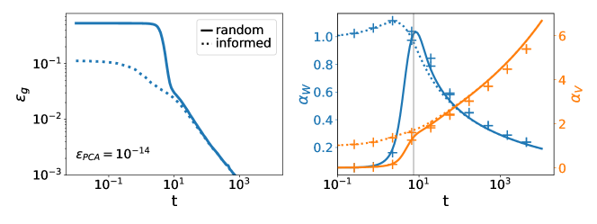
Figure 10: Learning in non-linear shallow AE occurs in two phases (a) The $\operatorname{\sf pmse}$ of an auto-encoder trained from random initial conditions first decays exponentially and then as a power law in time. Dynamics of the scaling constants $\alpha_{v}$ and $\alpha_{w}$ The reduced set of $2K$ ODEs match the results of simulations. The dynamics of an AE initialised randomly with random initial conditions become indistinguishable with those of an AE whose weights are initialised proportional to the PCs. This shows that the network first recovers the leading PCs subspace and then adjusts the norm of the weights in order to recover the linear regime. Parameters: $\eta=1,K=64,bs=1$

To validate our calculations for autoencoders with finite $D$, we trained an autoencoder from three distinct initial conditions: A random one, an informed configuration in which the weights are initialised as in Eq. 19 with $\alpha_{v}^{k}=\alpha_{w}^{k}=1$ and a perfect one, in which additionally, $\alpha_{v}^{k}$ is initialised from the minimal $\operatorname{\sf pmse}$ solution Eq. C.6. The first observation is that the $\operatorname{\sf pmse}$ of the network started with perfect initial conditions remains at the PCA reconstruction error, thus validating Eq. C.6. Since we have a noiseless dataset, the PCA error is given by the numerical error, however we note that the same conclusion caries over to noisy datasets with finite PCA reconstruction error. In fig. 10, we plot the $\operatorname{\sf pmse}$ of the randomly initialised and informed autoencoders on the left as well as the evolution of $\alpha_{v}^{k}$ and $\alpha_{w}^{k}$, i.e. of the overlap between the weights and the eigenvectors during training, on the right. We can see that the network with random initial weights learns in two phases: first the $\operatorname{\sf pmse}$ decays exponentially until it reaches the error of the aligned network. Then, its $\operatorname{\sf pmse}$ coincides with that of the informed network and the error decays as a power-law. This shows that during the first phase of exponential learning, the network recovers the leading PC subspace. This occurs early on in training. In the second phase, the networks adjust the norm of the weights to reach PCA performances. As discussed in the main text, this is achieved in the sigmoidal network by shrinking the encoder’s weights, so as to recover the linear regime of the activation function. It keeps the norm of the reconstruction similar to the one of the input by and growing the decoder’s weights.

Appendix D Analytical formula of the integral

In this subsection we define $C=(c_{ij})_{i,j=1,..,k}$ the covariance matrix of the variables $\{x_{i}\}_{i=1,..,k}$ appearing in the expectation. For e.g. $\mathbb{E}\,x_{1}x_{2}-\mathbb{E}\,x_{1}\mathbb{E}\,x_{2}=c_{12}$.

Sigmoidal activation function

$$I_{2} \equiv\mathbb{E}\,g(x_{1})g(x_{2})=\frac{2}{\pi}\left[\frac{c_{12}}{\sqrt{1+c_{11}}\sqrt{1+c_{22}}}\right]$$ (D.1)

$$J_{2} \equiv\mathbb{E}\,x_{1}g(x_{2})=\sqrt{\frac{2}{\pi(1+c_{22})}}c_{12}$$ (D.2)

$$I_{3} \equiv\mathbb{E}\,g^{\prime}(x_{1})x_{2}g(x_{3})=\frac{2}{\pi}\frac{1}{\sqrt{(1+c_{11})(1+c_{33})-c_{13}^{2}}}\frac{c_{23}(1+c_{11})-c_{12}c_{13}}{1+c_{11}}$$ (D.3)

$$I_{21} \equiv\mathbb{E}\,g^{\prime}(x_{1})x_{1}x_{2}=\sqrt{\frac{2}{\pi}}\frac{c_{12}}{(c_{11}+1)^{3/2}}$$ (D.4)

$$I_{22} \equiv\mathbb{E}\,g^{\prime}(x_{1})x_{2}^{2}=\sqrt{\frac{2}{\pi}}\frac{\left(c_{11}c_{22}-c_{12}^{2}+c_{22}\right)}{(c_{11}+1)^{3/2}}$$ (D.5)

Linear activation function

$$I_{2}=J_{2}=I_{21}\equiv\mathbb{E}\,x_{1}x_{2}=c_{12}$$ (D.6)

$$I_{22}\equiv\mathbb{E}\,x_{2}^{2}=c_{22}$$ (D.7)

$$I_{3}\equiv\mathbb{E}\,x_{2}x_{3}=c_{23}$$ (D.8)

ReLU activation function

$$I_{2} \equiv\mathbb{E}\,g(x_{1})g(x_{2})=\frac{1}{8\pi}\left[2\sqrt{c_{11}c_{22}-c_{12}^{2}}+c_{12}\pi+2c_{12}+\arctan{\frac{c_{12}}{\sqrt{c_{11}c_{22}-c_{12}^{2}}}}\right]$$ (D.10)

$$J_{2} \equiv\mathbb{E}\,x_{1}g(x_{2})=\frac{c_{12}}{2}$$ (D.11)

References

- Baldi & Hornik (1989) Baldi, P. and Hornik, K. Neural networks and principal component analysis: Learning from examples without local minima. Neural networks, 2(1):53–58, 1989.
- Bao et al. (2020) Bao, X., Lucas, J., Sachdeva, S., and Grosse, R. B. Regularized linear autoencoders recover the principal components, eventually. In Larochelle, H., Ranzato, M., Hadsell, R., Balcan, M. F., and Lin, H. (eds.), Advances in Neural Information Processing Systems, volume 33, pp. 6971–6981. Curran Associates, Inc., 2020. URL https://proceedings.neurips.cc/paper/2020/file/4dd9cec1c21bc54eecb53786a2c5fa09-Paper.pdf.
- Biehl & Schlösser (1998) Biehl, M. and Schlösser, E. The dynamics of on-line principal component analysis. Journal of Physics A: Mathematical and General, 31(5):L97–L103, 1998. doi: 10.1088/0305-4470/31/5/002. URL https://doi.org/10.1088/0305-4470/31/5/002.
- Bishop (2006) Bishop, C. Pattern recognition and machine learning. Springer, New York, 2006.
- Bourlard & Kamp (1988) Bourlard, H. and Kamp, Y. Auto-association by multilayer perceptrons and singular value decomposition. Biological cybernetics, 59(4):291–294, 1988.
- Chizat et al. (2019) Chizat, L., Oyallon, E., and Bach, F. On lazy training in differentiable programming. In Advances in Neural Information Processing Systems, pp. 2937–2947, 2019.
- Eckart & Young (1936) Eckart, C. and Young, G. The approximation of one matrix by another of lower rank. Psychometrika, 1(3):211–218, 1936.
- Gidel et al. (2019) Gidel, G., Bach, F., and Lacoste-Julien, S. Implicit regularization of discrete gradient dynamics in linear neural networks. In Wallach, H., Larochelle, H., Beygelzimer, A., d'Alché-Buc, F., Fox, E., and Garnett, R. (eds.), Advances in Neural Information Processing Systems, volume 32. Curran Associates, Inc., 2019. URL https://proceedings.neurips.cc/paper/2019/file/f39ae9ff3a81f499230c4126e01f421b-Paper.pdf.
- Goldt et al. (2019) Goldt, S., Advani, M., Saxe, A., Krzakala, F., and Zdeborová, L. Dynamics of stochastic gradient descent for two-layer neural networks in the teacher-student setup. In Advances in Neural Information Processing Systems 32, 2019.
- Goldt et al. (2020) Goldt, S., Mézard, M., Krzakala, F., and Zdeborová, L. Modeling the influence of data structure on learning in neural networks: The hidden manifold model. Phys. Rev. X, 10(4):041044, 2020.
- Goldt et al. (2022) Goldt, S., Loureiro, B., Reeves, G., Krzakala, F., Mezard, M., and Zdeborova, L. The gaussian equivalence of generative models for learning with shallow neural networks. In Bruna, J., Hesthaven, J., and Zdeborova, L. (eds.), Proceedings of the 2nd Mathematical and Scientific Machine Learning Conference, volume 145 of Proceedings of Machine Learning Research, pp. 426–471. PMLR, 2022.
- Gunasekar et al. (2017) Gunasekar, S., Woodworth, B., Bhojanapalli, S., Neyshabur, B., and Srebro, N. Implicit Regularization in Matrix Factorization. In Advances in Neural Information Processing Systems 30, pp. 6151–6159, 2017.
- Horn & Johnson (2012) Horn, R. A. and Johnson, C. R. Matrix analysis. Cambridge university press, 2012.
- Hu & Lu (2020) Hu, H. and Lu, Y. M. Universality laws for high-dimensional learning with random features. arXiv:2009.07669, 2020.
- Jacot et al. (2018) Jacot, A., Gabriel, F., and Hongler, C. Neural tangent kernel: Convergence and generalization in neural networks. In Advances in Neural Information Processing Systems 32, pp. 8571–8580, 2018.
- Krizhevsky et al. (2009) Krizhevsky, A., Hinton, G., et al. Learning multiple layers of features from tiny images. arXiV preprint, 2009. URL https://www.cs.toronto.edu/~kriz/learning-features-2009-TR.pdf.
- Kunin et al. (2019) Kunin, D., Bloom, J., Goeva, A., and Seed, C. Loss landscapes of regularized linear autoencoders. In Chaudhuri, K. and Salakhutdinov, R. (eds.), Proceedings of the 36th International Conference on Machine Learning, volume 97 of Proceedings of Machine Learning Research, pp. 3560–3569. PMLR, 2019. URL https://proceedings.mlr.press/v97/kunin19a.html.
- Liao & Couillet (2018) Liao, Z. and Couillet, R. On the spectrum of random features maps of high dimensional data. In International Conference on Machine Learning, pp. 3063–3071. PMLR, 2018.
- Loureiro et al. (2021) Loureiro, B., Gerbelot, C., Cui, H., Goldt, S., Krzakala, F., Mézard, M., and Zdeborová, L. Learning curves of generic features maps for realistic datasets with a teacher-student model. In Advances in Neural Information Processing Systems, volume 34, 2021.
- Marchenko & Pastur (1967) Marchenko, V. and Pastur, L. Distribution of eigenvalues for some sets of random matrices. Matematicheskii Sbornik, 114(4):507–536, 1967.
- Mei & Montanari (2021) Mei, S. and Montanari, A. The generalization error of random features regression: Precise asymptotics and the double descent curve. Communications on Pure and Applied Mathematics, 2021. doi: https://doi.org/10.1002/cpa.22008. URL https://onlinelibrary.wiley.com/doi/abs/10.1002/cpa.22008.
- Mianjy et al. (2018) Mianjy, P., Arora, R., and Vidal, R. On the implicit bias of dropout. In Dy, J. and Krause, A. (eds.), Proceedings of the 35th International Conference on Machine Learning, volume 80 of Proceedings of Machine Learning Research, pp. 3540–3548. PMLR, 2018. URL https://proceedings.mlr.press/v80/mianjy18b.html.
- Nakkiran et al. (2021) Nakkiran, P., Neyshabur, B., and Sedghi, H. The bootstrap framework: Generalization through the lens of online optimization. In International Conference on Learning Representations, 2021. URL https://openreview.net/forum?id=guetrIHLFGI.
- Nguyen (2021) Nguyen, P.-M. Analysis of feature learning in weight-tied autoencoders via the mean field lens. arXiv preprint arXiv:2102.08373, 2021.
- Nguyen et al. (2019) Nguyen, T. V., Wong, R. K., and Hegde, C. On the dynamics of gradient descent for autoencoders. In The 22nd International Conference on Artificial Intelligence and Statistics, pp. 2858–2867. PMLR, 2019.
- Oftadeh et al. (2020) Oftadeh, R., Shen, J., Wang, Z., and Shell, D. Eliminating the invariance on the loss landscape of linear autoencoders. In III, H. D. and Singh, A. (eds.), Proceedings of the 37th International Conference on Machine Learning, volume 119 of Proceedings of Machine Learning Research, pp. 7405–7413. PMLR, 07 2020. URL https://proceedings.mlr.press/v119/oftadeh20a.html.
- Oja (1982) Oja, E. Simplified neuron model as a principal component analyzer. Journal of mathematical biology, 15(3):267–273, 1982.
- Plaut (2018) Plaut, E. From principal subspaces to principal components with linear autoencoders. arXiv preprint arXiv:1804.10253, 2018.
- Potters & Bouchaud (2020) Potters, M. and Bouchaud, J.-P. A First Course in Random Matrix Theory: For Physicists, Engineers and Data Scientists. Cambridge University Press, 2020.
- Pretorius et al. (2018) Pretorius, A., Kroon, S., and Kamper, H. Learning dynamics of linear denoising autoencoders. In International Conference on Machine Learning, pp. 4141–4150. PMLR, 2018.
- Refinetti et al. (2021) Refinetti, M., Goldt, S., Krzakala, F., and Zdeborova, L. Classifying high-dimensional gaussian mixtures: Where kernel methods fail and neural networks succeed. In Meila, M. and Zhang, T. (eds.), Proceedings of the 38th International Conference on Machine Learning, volume 139 of Proceedings of Machine Learning Research, pp. 8936–8947. PMLR, 2021. URL https://proceedings.mlr.press/v139/refinetti21b.html.
- Riegler & Biehl (1995) Riegler, P. and Biehl, M. On-line backpropagation in two-layered neural networks. Journal of Physics A: Mathematical and General, 28(20), 1995.
- Saad (2009) Saad, D. On-line learning in neural networks, volume 17. Cambridge University Press, 2009.
- Saad & Solla (1995a) Saad, D. and Solla, S. Exact Solution for On-Line Learning in Multilayer Neural Networks. Phys. Rev. Lett., 74(21):4337–4340, 1995a.
- Saad & Solla (1995b) Saad, D. and Solla, S. On-line learning in soft committee machines. Phys. Rev. E, 52(4):4225–4243, 1995b.
- Sanger (1989) Sanger, T. D. Optimal unsupervised learning in a single-layer linear feedforward neural network. Neural networks, 2(6):459–473, 1989.
- Saxe et al. (2019) Saxe, A., McClelland, J., and Ganguli, S. A mathematical theory of semantic development in deep neural networks. Proceedings of the National Academy of Sciences, 116(23):11537–11546, 2019.
- Schlösser et al. (1999) Schlösser, E., Saad, D., and Biehl, M. Optimization of on-line principal component analysis. Journal of Physics A: Mathematical and General, 32(22):4061–4067, 1999. doi: 10.1088/0305-4470/32/22/306. URL https://doi.org/10.1088/0305-4470/32/22/306.
- Seddik et al. (2019) Seddik, M., Tamaazousti, M., and Couillet, R. Kernel random matrices of large concentrated data: the example of gan-generated images. In ICASSP 2019-2019 IEEE International Conference on Acoustics, Speech and Signal Processing (ICASSP), pp. 7480–7484. IEEE, 2019.
- Veiga et al. (2022) Veiga, R., Stephan, L., Loureiro, B., Krzakala, F., and Zdeborová, L. Phase diagram of stochastic gradient descent in high-dimensional two-layer neural networks. arXiv preprint arXiv:2202.00293, 2022.
- Wishart (1928) Wishart, J. The generalised product moment distribution in samples from a normal multivariate population. Biometrika, 20(1/2):32–52, 1928.
- Xiao et al. (2017) Xiao, H., Rasul, K., and Vollgraf, R. Fashion-mnist: a novel image dataset for benchmarking machine learning algorithms. arXiV preprint, 2017. URL https://arxiv.org/pdf/1708.07747.pdf.
- Yoshida & Okada (2019) Yoshida, Y. and Okada, M. Data-dependence of plateau phenomenon in learning with neural network — statistical mechanical analysis. In Advances in Neural Information Processing Systems 32, pp. 1720–1728, 2019.