Nondivergent deflection of light around a photon sphere of a compact object

Abstract

We demonstrate that the location of a stable photon sphere (PS) in a compact object is not always an edge such as the inner boundary of a black hole shadow, whereas the location of an unstable PS is known to be the shadow edge notably in the Schwarzschild black hole. If a static spherically symmetric (SSS) spacetime has the stable outermost PS, the spacetime cannot be asymptotically flat. A nondivergent deflection is caused for a photon traveling around a stable PS, though a logarithmic divergent behavior is known to appear in most of SSS compact objects with an unstable photon sphere. The reason for the nondivergence is that the closest approach of a photon is prohibited in the immediate vicinity of the stable PS when the photon is emitted from a source (or reaches a receiver) distant from a lens object. The finite gap size depends on the receiver and source distances from the lens as well as the lens parameters. The mild deflection angle of light can be approximated by an arcsine function. A class of SSS solutions in Weyl gravity exemplify the nondivergent deflection near the stable outer PS.

I Introduction

Since the first measurement by Eddington and his collaborators Eddington , the gravitational deflection of light has offered us a powerful tool for tests of gravitational theories including the theory of general relativity as well as for astronomical probes of dark matter. The Event Horizon Telescope (EHT) team has recently succeeded in taking a direct image of the immediate vicinity of the central black hole candidate of M87 galaxy EHT . In addition, the same team has just reported measurements of linear polarizations around the same black hole candidate EHT2021a , which has led to an estimation of the mass accretion rate EHT2021b . These observations have increased our renewed interest in the strong deflection of light in the strong gravity region.

The strong deflection of light by Schwarzschild black hole was pointed out by Darwin Darwin . This phenomena is closely related with a photon sphere (PS) that, with a horizon, features black holes and other compact objects Perlick ; CVE ; Bozza2002 ; Hod2013 ; Sanchez ; DFR ; WLG ; SYG ; CGP ; Tsukamoto2017 ; GW2016 ; Ohgami2015 ; Koga2016 ; Koga2018 ; Koga2019 ; Koga2020 ; Koga2021 ; Tsukamoto2020 ; Shiromizu ; Yoshino2017 ; Yoshino2020a ; Yoshino2020b ; Yang2020 ; Tsukamoto2021a ; Izumi2021 ; Tsukamoto2021b ; CG2016 ; Mishra2019 ; CG2021 ; Guo2021 ; Konoplya2021 ; Gan2021 ; Ghosh2021 ; Siino2021a ; Siino2021b . A photon surface for a less symmetric case is a generalization of PSs CVE .

Many years later, Bozza showed that the strong deflection behavior in Schwarzschild black hole can be well described as the logarithmic divergence in the deflection angle Bozza2002 . Such a strong deflection as the logarithmic divergence occurs also in other exotic objects such as wormholes. For instance, Tsukamoto conducted several extensions of Bozza method for the strong deflection of light Tsukamoto2017 ; Tsukamoto2020 , in which the logarithmic behavior is shown to be a quite general feature for a static and spherically symmetric (SSS) compact object that has a PS, e.g. Ellis wormholes. The logarithmic behavior in the strong deflection for a finite-distance receiver and source has been recently confirmed Takizawa2021 by solving the exact gravitational lens that stands even for an asymptotically nonflat spacetime Bozza2008 ; Takizawa2020a ; Takizawa2020b .

There exists a single PS outside the horizon of the Schwarzschild black hole, while Ellis wormhole has a PS without horizons. For both cases, the number of PSs is one. Tsukamoto obtained the logarithmic behavior for such a SSS spacetime with a single PS, which was assumed to be unstable. In both of Schwarzschild black hole and Ellis wormhole, there exists only the unstable PS. Cunha et al. have recently proven that ultra-compact objects have an even number of PSs, one of which is stable Cunha . Regarding the interesting theorem, Hod has found an exception for horizonless spacetimes that possess no stable PS Hod2018 . What happens, if the PS is stable and a light ray is deflected around the stable PS?

The main purpose of the present paper is to study the deflection of light around a PS when the PS is stable in a SSS spacetime. This situation has not often been considered in detail e.g. Darwin ; Bozza2002 ; Tsukamoto2017 ; Tsukamoto2021a ; Tsukamoto2021b , except for Hasse and Perlick (2002) HP that provided a theorem on a connection among three properties of (1) the presence of a PS for a saddle point case and a stable case as well as an unstable one, (2) the centrifugal force reversal and (3) infinitely many images in any SSS spacetime. Hasse and Perlick (2002), however, did not calculate the deflection angle of light, because they focused on the multiple imaging HP . We shall show that, in stead of the logarithmic type of the strong deflection, a mild deflection is caused near the stable PS.

This paper is organized as follows. In Section II, we reexamine the deflection angle of light when there exists a stable outer PS in a SSS spacetime. In Section III, we study how light is deflected in the presence of the stable outer PS. It is shown that the deflection behavior is not too strong to make the logarithmic divergence but mild enough to be approximated by an arcsine function. As an example for such a mild deflection of light, we consider a class of Weyl gravity model in Section IV. Section V concludes the present paper. Throughout this paper, we use the unit of $G=c=1$.

II Deflection angle integral

II.1 SSS spacetime

We consider a SSS spacetime, for which the metric reads

$$ds^{2}=-A(r)dt^{2}+B(r)dr^{2}+C(r)(d\theta^{2}+\sin^{2}\theta d\phi^{2}),$$ (1)

where $A(r)>0$, $B(r)>0$, and $C(r)>0$ are assumed to be finite. If the SSS spacetime possesses a horizon, we focus on the outside of the horizon. We do not assume the asymptotic flatness of the spacetime. Actually, the present paper considers an asymptotically nonflat case. A lemma on this issue is given at the end of the present section.

II.2 Photon orbits

Without loss of generality, we can consider a photon orbit on the equatorial plane $(\theta=\pi/2)$ because of the spherical symmetry of the spacetime. On the equatorial plane in the SSS spacetime, a light ray has two constants of motion. One is the specific energy $E\equiv A(r)\dot{t}$ and the other is the specific angular momentum $L\equiv C(r)\dot{\phi}$, where the overdot denotes the derivative with respect to the affine parameter $\lambda$ along the light ray.

By using the two constants $E$ and $L$, the impact parameter of light becomes $b=L/E$. Without loss of generality, we assume $b>0$.

In terms of $b$, the null condition $ds^{2}=0$ is rearranged as the orbit equation

$$\dot{r}^{2}+V(r)=0,$$ (2)

where $V(r)$ is defined as

$$V(r)\equiv-\frac{L^{2}F(r)}{B(r)C(r)}.$$ (3)

Here,

$$F(r)\equiv\frac{C(r)}{A(r)b^{2}}-1.$$ (4)

The closest approach of a light ray is denoted as $r_{0}$, which satisfies $V(r_{0})=0$ from the definition of $r_{0}$. Henceforth, evaluation at $r=r_{0}$ is indicated by the subscript $0$. For instance, $V(r_{0})=0$ is equivalent to $F_{0}=0$, where $F_{0}\equiv F(r_{0})$. By combining $F_{0}=0$ and Eq. (4), we obtain

$$b=\sqrt{\frac{C_{0}}{A_{0}}}.$$ (5)

This offers a relation between $b$ and $r_{0}$.

Following Hasse and Perlick HP , we use a particular form of the potential $\tilde{V}(r)$ that is defined as

$$\tilde{V}(r)\equiv\frac{A(r)}{C(r)},$$ (6)

which is conformally invariant. Thereby Eq. (2) is rewritten as

$$A(r)B(r)\dot{r}^{2}+L^{2}\tilde{V}(r)-E^{2}=0.$$ (7)

This simplifies the analysis of the photon sphere and its linear perturbation, because $V(r)$ depends on $b$ as well as $r$, whereas $\tilde{V}(r)$ does not include $b$. The potential $\tilde{V}(r)$ plays the central role in the proof of a theorem that clarifies a connection among three properties of the presence of a PS, the centrifugal force reversal and infinitely many images in any SSS spacetime HP .

For the later convenience, we write down the first and second derivatives of $\tilde{V}(r)$,

$$\tilde{V}^{{}^{\prime}}(r)= -\frac{A(r)D(r)}{C(r)},$$ (8)

$$\tilde{V}^{{}^{\prime\prime}}(r)= -\frac{A(r)}{C(r)}\left[D^{{}^{\prime}}(r)-D(r)^{2}\right],$$ (9)

where the prime denotes the differentiation with respect to $r$, and the functions $D$ is defined as

$$D(r) \equiv\frac{C^{\prime}(r)}{C(r)}-\frac{A^{\prime}(r)}{A(r)}.$$ (10)

From Eq. (7), we obtain

$$[A(r)B(r)]^{{}^{\prime}}\dot{r}^{2}+2A(r)B(r)\ddot{r}+L^{2}\tilde{V}^{{}^{\prime}}(r)=0.$$ (11)

Eqs. (7) and (11) tell that a photon orbit is a circle if and only if $r=r_{m}$ satisfies $\tilde{V}(r_{m})=(b_{m})^{-2}$ and $\tilde{V}^{{}^{\prime}}(r_{m})=0$, where $r_{m}$ denotes the radius of the PS and the subscript $m$ denotes the value at $r=r_{m}$. From $\tilde{V}(r_{m})=(b_{m})^{-2}$, the impact parameter for the PS is obtained as

$$b_{m}=\sqrt{\frac{C_{m}}{A_{m}}},$$ (12)

where Eq. (6) is used.

II.3 Classification of PS stability

We consider a small displacement $\delta r$ around the PS orbit, $r=r_{m}+\delta r$. At the linear order in $\delta r$, Eq, (11) gives

$$\frac{d^{2}}{d\lambda^{2}}(\delta r) =-\frac{L^{2}\tilde{V}^{{}^{\prime\prime}}(r_{m})}{2A_{m}B_{m}}\delta r$$

$$=\frac{L^{2}D^{{}^{\prime}}_{m}}{2B_{m}C_{m}}\delta r,$$ (13)

where Eq. (9) and $D(r_{m})=0$ from $\tilde{V}^{{}^{\prime}}(r_{m})=0$ are used.

The linear stability of the perturbed orbit is determined only by the sign of $D_{m}^{{}^{\prime}}$, because $A(r)>0$, $B(r)>0$, $C(r)>0$ and $L\neq 0$. A PS is stable if $D_{m}^{{}^{\prime}}<0$, whereas it is unstable for $D_{m}^{{}^{\prime}}>0$.

From Eq. (10), we obtain

$$D^{{}^{\prime}}(r)=\frac{C^{\prime\prime}(r)}{C(r)}-\frac{A^{\prime\prime}(r)}{A(r)}-D(r)\left(\frac{C^{\prime}(r)}{C(r)}+\frac{A^{\prime}(r)}{A(r)}\right).$$ (14)

On the PS, this is reduced to

$$D^{\prime}_{m}=\frac{C_{m}^{\prime\prime}}{C_{m}}-\frac{A_{m}^{\prime\prime}}{A_{m}}.$$ (15)

Bozza and Tsukamoto assumed $D^{\prime}_{m}>0$, which means an unstable PS Bozza2002 ; Tsukamoto2017 . Henceforth, we focus on a stable case $D^{\prime}_{m}<0$. Such an unusual case is realized in a class of Weyl gravity model as shown in Section VI.

II.4 Total angle integral

From Eq. (2), we obtain

$$\frac{dr}{d\phi}=\pm\sqrt{\frac{C(r)F(r)}{B(r)}},$$ (16)

for which we choose the plus sign without loss of generality. Integrating this from a source (denoted as S) to a receiver (denoted as R) leads to the total change in the longitudinal angle.

$$I_{F}(r_{S},r_{R},r_{0}) \equiv\sum_{i=S,R}\int_{r_{0}}^{r_{i}}\frac{dr}{\sqrt{\frac{C(r)F(r)}{B(r)}}}.$$ (17)

Note that a conventional method discusses the total integral $I$ for the asymptotic receiver and source ($r_{R}\to\infty$ and $r_{S}\to\infty$) e.g. Darwin ; Bozza2002 ; Tsukamoto2017 , for which $I-\pi$ gives the deflection angle of light. On the other hand, the present paper considers finite distance between the receiver and source. In order to clarify this difference, we use $I_{F}$ in stead of $I$. Rigorously speaking, $I_{F}-\pi$ is not the deflection angle but $I_{F}$ is the dominant component of the deflection angle. This issue is beyond the scope of this paper. See e.g. References Ishihara2016 ; Ishihara2017 ; Ono2017 ; Ono2019U on how to define geometrically the deflection angle for the finite-distance receiver and source.

Following Bozza and Tsukamoto Bozza2002 ; Tsukamoto2017 , we introduce a variable as

$$z\equiv 1-\frac{r_{0}}{r},$$ (18)

to rewrite Eq. (17) as

$$I_{F}(z_{S},z_{R},r_{0})=\sum_{i=S,R}\int_{0}^{z_{i}}f(z,r_{0})dz,$$ (19)

where we define $z_{i}\equiv 1-r_{0}/r_{i}$ $(i=R,S)$,

$$H(z,r_{0}) \equiv\frac{CF}{B}(1-z)^{4},$$ (20)

and

$$f(z,r_{0}) \equiv\frac{r_{0}}{\sqrt{H(z,r_{0})}}.$$ (21)

In the next subsection, we shall examine the integrand in Eq. (19).

II.5 Analysis in the vicinity of PS

By noting $F_{0}=0$, the function $H$ is expanded around $r=r_{0}$ ($z=0$) as

$$H(z,r_{0})=\sum_{n=1}^{\infty}c_{n}(r_{0})z^{n},$$ (22)

where

$$c_{1}(r_{0}) =\frac{C_{0}D_{0}r_{0}}{B_{0}},$$ (23)

$$c_{2}(r_{0}) =\frac{C_{0}}{B_{0}}\left[D_{0}r_{0}\left(\frac{C^{\prime}_{0}}{C_{0}}-\frac{B^{\prime}_{0}}{B_{0}}-3\right)+\frac{r_{0}^{2}}{2}(D_{0}^{2}+D^{\prime}_{0})\right],$$ (24)

$$c_{3}(r_{0}) =\frac{C_{0}}{B_{0}}\left[D_{0}r_{0}\left(\frac{3B^{\prime}_{0}r_{0}}{B_{0}}-\frac{3C^{\prime}_{0}r_{0}}{C_{0}}-\frac{B^{\prime}_{0}C^{\prime}_{0}r_{0}^{2}}{B_{0}C_{0}}-3\right)\right.$$

$$~{}~{}~{}~{}~{}~{}~{}~{}~{}+\frac{r_{0}^{2}}{2}(D_{0}^{2}+D^{\prime}_{0})\left(\frac{C^{\prime}_{0}r_{0}}{C_{0}}-\frac{B^{\prime}_{0}r_{0}}{B_{0}}-2\right)$$

$$~{}~{}~{}~{}~{}~{}~{}~{}~{}\left.+\frac{r_{0}^{3}}{6}\left(D_{0}^{3}+3D^{\prime}_{0}D_{0}+D^{\prime\prime}_{0}\right)\right].$$ (25)

When the closest approach is located near the PS ($r_{0}=r_{m}$), Eqs. (23) - (25) become

$$c_{1}(r_{m}) =0,$$ (26)

$$c_{2}(r_{m}) =\frac{r_{m}^{2}C_{m}D_{m}^{\prime}}{2B_{m}},$$ (27)

$$c_{3}(r_{m}) =\frac{r_{m}^{2}C_{m}}{2B_{m}}\left[D_{m}^{\prime}\left(\frac{C_{m}^{\prime}r_{m}}{C_{m}}-\frac{B_{m}^{\prime}r_{m}}{B_{m}}-2\right)+\frac{r_{m}D_{m}^{\prime\prime}}{3}\right].$$ (28)

From Eqs. (26) - (28), we find

$$H(z,r_{m})=c_{2}(r_{m})z^{2}+O(z^{3}).$$ (29)

If the PS is unstable (stable), namely $D^{{}^{\prime}}_{m}>0$ ($D^{{}^{\prime}}_{m}<0$), then, $c_{2}(r_{m})>0$ ($<0$). As pointed by Tsukamoto Tsukamoto2017 , the angle integral $I_{F}$ by Eq. (17) is divergent logarithmically. On the other hand, the stable PS case ($c_{2}(r_{m})<0$) is investigated below in detail.

Before closing this section, we mention a relation of the emergence of the stable outermost PS (SOPS) and the spacetime asymptotic flatness.

Lemma
If a SSS spacetime has the SOPS, the spacetime cannot be asymptotically flat, for which $\tilde{V}^{{}^{\prime}}(r)=[A(r)/C(r)]^{{}^{\prime}}$ is positive everywhere outside the SOPS.

Proof
We denote the radius of the SOPS as $r_{SOPS}$. At the location of the SOPS, $\tilde{V}^{{}^{\prime}}(r_{SOPS})=0$ and $\tilde{V}^{{}^{\prime\prime}}(r_{SOPS})>0$. There exist no PSs outside of the SOPS, because the SOPS is the outermost PS. Therefore, $\tilde{V}^{{}^{\prime\prime}}(r)>0$ for $r>r_{SOPS}$. This means that $\tilde{V}^{{}^{\prime}}(r)$ is an increasing function of $r$ when $r>r_{SOPS}$. Hence, $\tilde{V}^{{}^{\prime}}(r)>0$ for $r>r_{SOPS}$.

Here, we add an assumption that the spacetime were asymptotically flat. Then, we can employ a coordinate system in which Eq. (1) approaches the Minkowski metric in the polar coordinates asymptotically as $r\to\infty$. Namely, $A(r)\to 1+O(1/r)$ and $C(r)\to r^{2}+O(r)$, which lead to $A^{{}^{\prime}}(r)\to O(1/r^{2})$ and $C^{{}^{\prime}}(r)\to 2r+O(r^{0})$. Thereby,

$$\tilde{V}^{{}^{\prime}}(r) =\left(\frac{A(r)}{C(r)}\right)^{{}^{\prime}}$$

$$=-\frac{2}{r^{3}}+O\left(\frac{1}{r^{4}}\right)$$

$$\to 0,$$ (30)

in the limit as $r\to\infty$. This means that $\tilde{V}^{{}^{\prime}}(r)$ has an extremum between $r_{SOPS}$ and $r=\infty$, because of its continuity. This contradicts with that $\tilde{V}^{{}^{\prime}}(r)$ is an increasing function for $r>r_{SOPS}$. Therefore, the spacetime is not asymptotically flat. A proof of the lemma is thus completed.

According to Reference Guo2021 , if an axisymmetric, stationary and asymptotically flat spacetime posses light rings (LRs), the outest LR is unstable. This means that if a SSS spacetime with PSs is asymptotically flat, the outest PS is unstable. The contraposition of this is that, if the outest PS in a SSS spacetime with PSs is stable, the spacetime is not asymptotically flat. This proves a part of the above lemma but tells nothing about the positivity of $\tilde{V}^{{}^{\prime}}(r)$ for $r>r_{SOPS}$.

On the other hand, it is clear that the asymptotic flatness is allowed, if the outermost PS (OPS) is unstable ($\tilde{V}^{{}^{\prime\prime}}(r_{OPS})<0$). In the rest of this paper, we consider that a receiver and source are located outside of a stable outer PS. However, it is not specified below whether or not it is the outermost.

Before closing the section, let us briefly mention the stability of a spacetime that admits a stable PS. Horizonless ultracompact objects with a stable PS may suffer from instabilities due to slowly (at most logarithmically) decaying of perturbations leading to the formation of a trapped surface Cardoso2014 ; Keir ; Cunha ; AMY . In section VI, therefore, we consider a black hole model with a stable PS in Weyl gravity. On the other hand, the above lemma may suggest another possibility compatible with the instability arguments in References Cardoso2014 ; Keir ; Cunha ; AMY . One such candidate is a compact object without a black hole horizon but with a stable PS and a cosmological horizon that is consistent with the asymptotic nonflatness. Its stability issue is beyond the scope of the present paper.

III Mild deflection near the stable outer PS

III.1 Stability classification of the outer PS

In the neighborhood of the closest approach $z\sim 0$, higher order terms of $H(z,r_{m})$ in Eq. (22) are negligible compared with $z$ and $z^{2}$ terms. The dominant part of $f(z,r_{0})$ for $r_{0}\sim r_{m}$ thus becomes

$$f_{D}(z,r_{0})\equiv\frac{r_{0}}{\sqrt{h(z)}},$$ (31)

where $h(z)$ is defined as

$$h(z)=c_{1}(r_{0})z+c_{2}(r_{0})z^{2}.$$ (32)

Associated with $f_{D}(z,r_{0})$, we define the dominant part of the total angle integral as

$$I_{FD}(z_{R},z_{S},r_{0})\equiv\sum_{i=S,R}\int_{0}^{z_{i}}f_{D}(z,r_{0})dz.$$ (33)

Before starting calculations of the angle integral, first we investigate a photon orbit in the stable PS case. If $c_{1}(r_{0})<0$, $h(z)$ is always negative for $z>0$. This is in contradiction with the nonnegativity of $h(z)$. Hence, the case of $c_{1}(r_{0})<0$ is discarded. If $c_{1}(r_{0})=0$, then, $h(z)=c_{2}(r_{0})z^{2}$. The nonnegativity of $h(z)$ together with $c_{2}(r_{0})<0$ admits only $z=0$. This orbit is a circle. We do not discuss this special case any more. For the last case $c_{1}(r_{0})>0$, the nonnegativity of $h(z)$ provides a nontrivial situation; the allowed region for $z$ is

$$0\leq z\leq-\frac{c_{1}(r_{0})}{c_{2}(r_{0})}.$$ (34)

This means that only bound orbits are allowed, whereas the scattering orbits are prohibited. Note that $h(z)=0$ does not make the integral in Eq. (33) divergent. Indeed, $h(z)\sim c_{1}(r_{0})z$ near a point $z=0$ and $h(z)\sim-c_{1}(r_{0})[z+c_{1}(r_{0})/c_{2}(r_{0})]$ near a point $z\sim-c_{1}(r_{0})/c_{2}(r_{0})$. At the two points, therefore, the integral of $h(z)$ is not divergent as $\sim\int z^{-1/2}dz\sim 2\sqrt{z}$. The two points $z=0$ and $z\sim-c_{1}(r_{0})/c_{2}(r_{0})$ are the periastron and apastron, respectively.

III.2 Angle integral for the stable outer PS

Henceforth, we focus on the case of $c_{1}(r_{0})>0$, for which the receiver and source positions satisfy

$$0<z_{i}\leq-\frac{c_{1}(r_{0})}{c_{2}(r_{0})}.$$ (35)

Eq. (33) is integrated as

$$I_{FD}(z_{R},z_{S},r_{0})= \frac{r_{0}}{\sqrt{-c_{2}(r_{0})}}$$

$$\times\left[\pi-\sum_{i=S,R}\arcsin\left(1+\frac{2c_{2}(r_{0})}{c_{1}(r_{0})}z_{i}\right)\right].$$ (36)

It follows that the arcsine term in Eq. (36) is well defined for the allowed region by Eq. (35), because

$$-1\leq 1+\frac{2c_{2}(r_{0})}{c_{1}(r_{0})}z_{i}<1.$$ (37)

III.3 $I_{F}$ in terms of $b$

In most of lens studies including References Bozza2002 ; Tsukamoto2017 , it is convenient to express the deflection angle in terms of the impact parameter in stead to $r_{0}$, mainly because $b\sim D_{L}\theta$ for the lens distance $D_{L}$ and the image angle direction $\theta$.

Therefore, we look for an approximate expression of $b$. Near the PS, $c_{1}(r_{0})$ and $b(r_{0})$ are Taylor-expanded as

$$c_{1}(r_{0}) =\frac{C_{m}r_{m}D^{\prime}_{m}}{B_{m}}(r_{0}-r_{m})+O((r_{0}-r_{m})^{2}),$$ (38)

$$b(r_{0}) =b_{m}+\frac{b_{m}D^{\prime}_{m}}{4}(r_{0}-r_{m})^{2}+O((r_{0}-r_{m})^{3}).$$ (39)

From Eq. (38), we find

$$r_{0}<r_{m},$$ (40)

where $c_{1}(r_{0})>0$ and $D^{{}^{\prime}}_{m}<0$ are used. This inequality means that the light ray passes by the slight inside of the PS. This is because the PS is stable. This unusual behavior of the photon orbit implies also

$$b<b_{m},$$ (41)

from Eq. (39). See Figure 1 for the photon orbit behavior near the PS.

Figure 1: Schematic figure of photon orbits near a PS. The PS is denoted by a solid circle with radius $r_{m}$. The dotted circle has radius $r_{0}$, which is slightly smaller than $r_{m}$. Namely, $r_{m}-r_{0}$ is taken as a perturbation around the PS. The initial position of the photon is $r_{0}$, at which the initial radial velocity is vanishing. The thick dashed blue (in color) arrow denotes a photon motion when the PS is unstable. The orbital deviation grows because of being unstable. Therefore, it is difficult for the inner photon to escape to a far region. This is why the earlier papers focused on $r_{0}>r_{m}$ when an unstable PS is assumed Bozza2002 ; Tsukamoto2017 . On the other hand, the thick solid red (in color) arrow denotes a photon motion when the PS is stable. The orbital deviation gets smaller because of being stable. It is thus possible that the inner photon ($r_{0}<r_{m}$) crosses the PS to reach a distant observer.

By combining Eqs. (38) and (39), we obtain, near the PS, an approximate relation between $c_{1}(r_{0})$ and $b$ as

$$c_{1}(r_{0})\approx\frac{2r_{m}C_{m}\sqrt{-D^{\prime}_{m}}}{B_{m}}\left(1-\frac{b}{b_{m}}\right)^{\frac{1}{2}}.$$ (42)

By substituting this into Eq. (36), we obtain

$$I_{FD}(z_{R},z_{S},b)$$

$$\simeq\frac{r_{m}}{\sqrt{-c_{2}(r_{m})}}$$

$$~{}\times\left[\pi-\sum_{i=S,R}\arcsin\left\{1-\frac{r_{m}\sqrt{-D^{\prime}_{m}}}{2}\left(1-\frac{b}{b_{m}}\right)^{-\frac{1}{2}}z_{i}\right\}\right].$$ (43)

By direct calculations for a photon traveling near the PS, Eq. (35) is rearranged as

$$0<z_{i}\leq\frac{4}{r_{m}\sqrt{-D^{\prime}_{m}}}\left(1-\frac{b}{b_{m}}\right)^{1/2},$$ (44)

for which the arcsine function in Eq. (43) is well defined.

In order to obtain Eq. (43) as an approximate estimation of $I_{F}$ in terms of $b$, we have used the Taylor series expansion as Eq. (39), which is valid if $b_{m}>b_{m}|D^{{}^{\prime}}_{m}|(r_{0}-r_{m})^{2}/4$. This requires that the closest approach of light and the PS are close enough to satisfy

$$|r_{0}-r_{m}|<\frac{2}{\sqrt{|D^{{}^{\prime}}_{m}|}}.$$ (45)

Yet, a lower bound on $|r_{0}-r_{m}|$ exists in the neighborhood of the PS as shown below.

III.4 Discontinuity between the closest approach and the stable PS

Eq. (44) suggests a proposition on the existence of a gap between the allowed closest approach and the stable PS.

Proposition
In a SSS spacetime which possess a stable outer photon sphere, the closest approach of a photon from a source (or to a receiver) located at finite distance from the lens object is not allowed in the infinitesimal neighborhood of the stable PS.

Proof
This proposition can be proven by contradiction as follows. We consider a receiver (or a source) at finite distance from the lens, namely $r_{i}>r_{0}$, which leads to $z_{i}>0$. We assume the closest approach of a photon orbit were in the infinitesimal neighborhood of the stable PS.

On the stable PS, $F_{m}=F^{{}^{\prime}}_{m}=0$, while $F^{{}^{\prime\prime}}_{m}<0$. The last inequality comes from the unstable condition $D^{{}^{\prime}}_{m}<0$. The function $F$ near the PS is thus Taylor-expanded as

$$F_{0}=\frac{1}{2}F^{{}^{\prime\prime}}_{m}(r_{0}-r_{m})^{2}+O\left((r_{0}-r_{m})^{3}\right).$$ (46)

From Eq. (20), $H$ for $r_{0}\approx r_{m}$ is expanded as

$$H=\frac{C_{m}F^{{}^{\prime\prime}}_{m}}{2B_{m}}(1-z)^{4}(r_{0}-r_{m})^{2}+O\left((r_{0}-r_{m})^{3}\right),$$ (47)

where Eq. (46) is used.

By using $B_{m}>0$, $C_{m}>0$ and $F^{{}^{\prime\prime}}_{m}<0$ for Eq. (47), we find $H<0$ if $r_{0}-r_{m}$ is sufficiently small. $H<0$ contradicts with the existence of the photon orbit. Our proof is finished.

The above proposition prohibits the closest approach in the infinitesimal neighborhood of the stable PS. However, it does not tell about a size of the gap between the allowed closest approach and the stable PS. In order to discuss the gap size, we use Eq. (44), which is rewritten as

$$\frac{b}{b_{m}}\leq 1-\frac{r_{m}^{2}z_{i}^{2}(-D_{m}^{{}^{\prime}})}{16}.$$ (48)

Note that Eq. (44) is based on a quadratic approximation up to $z^{2}$.

For finite $z_{i}$ and $D_{m}^{{}^{\prime}}<0$, Eq. (48) demonstrates that $b$ is not allowed in the infinitesimal neighborhood of $b_{m}$. From Eq. (48), the upper bound on $b$ is

$$b_{max}=b_{m}-\frac{b_{m}r_{m}^{2}z_{L}^{2}(-D_{m}^{{}^{\prime}})}{16}.$$ (49)

The gap size $\Delta b\equiv b_{m}-b_{max}$ is thus given by

$$\Delta b=\frac{b_{m}r_{m}^{2}z_{L}^{2}(-D_{m}^{{}^{\prime}})}{16},$$ (50)

where $z_{L}$ is the larger one of $z_{R}$ and $z_{S}$, namely the value of $z$ for the more distant one of the receiver and source.

A separate treatment is needed for the marginal PSs ($D^{\prime}_{m}=0)$ e.g. CT ; Tsukamoto2020 .

III.5 The dominant part and the remainder

Before closing this section, we shall confirm that $I_{FR}\equiv I_{F}-I_{FD}$ is really the remainder. It is written simply as

$$I_{FR}(z_{R},z_{S},r_{0})\equiv\sum_{i=R,S}\int_{0}^{z_{i}}f_{R}(z,r_{0})dz,$$ (51)

where $f_{R}(z,r_{0})\equiv f(z,r_{0})-f_{D}(z,r_{0})$.

From Eq. (51), we obtain, for $z_{i}<1$,

$$I_{FR}(z_{R},z_{S},r_{0})=\sum_{i=R,S}[f_{R}(z_{i},r_{0})z_{i}+O(z_{i}^{2})].$$ (52)

For $r_{0}\sim r_{m}$, $f(z,r_{m})\sim f_{D}(z,r_{m})$ when $z<1$. Hence, by using the Taylor-expansion method, one may think that $f_{R}(z,r_{m})=f(z,r_{m})-f_{D}(z,r_{m})=O(z)$. However, let us more carefully examine an asymptotic expansion of $f_{R}(z,r_{0})$ for $z<1$ footnote-expansion . By straightforward calculations, the asymptotic expansion of $f(z,r_{0})$ for small $z$ is obtained as

$$f(z,r_{0})= \frac{r_{0}}{\sqrt{zc_{1}(r_{0})}}-\frac{r_{0}c_{2}(r_{0})}{2c_{1}(r_{0})^{3/2}}\sqrt{z}+O(z^{3/2}).$$ (53)

Similarly, the asymptotic expansion of $f_{D}(z,r_{0})$ is

$$f_{D}(z,r_{0})= \frac{r_{0}}{\sqrt{zc_{1}(r_{0})}}-\frac{r_{0}c_{2}(r_{0})}{2c_{1}(r_{0})^{3/2}}\sqrt{z}+O(z^{3/2}).$$ (54)

By bringing together Eqs. (53) and (54), we find

$$f_{R}(z,r_{0})=O(z^{3/2}).$$ (55)

By using this for Eq. (52), we find

$$I_{FR}(z_{R},z_{S},r_{0})=O(z_{R}^{5/2},z_{S}^{5/2}).$$ (56)

On the other hand, Eq. (36) is expanded, for small $z_{R}$ and $z_{S}$, as

$$I_{FD}(z_{R},z_{S},r_{0}) =\frac{2r_{0}}{\sqrt{c_{1}(r_{0})}}(\sqrt{z_{R}}+\sqrt{z_{S}})+O(z_{R},z_{S}),$$ (57)

where $\arcsin(1-\varepsilon)=\pi/2-\sqrt{2\varepsilon}+O(\varepsilon)$ is used.

For $z_{R},z_{S}\ll 1$, Eqs. (56) and (57) lead to $I_{FR}(z_{R},z_{S},r_{0})\ll I_{FD}(z_{R},z_{S},r_{0})$. Therefore, we can safely say that $I_{FD}$ is the dominant part and $I_{FR}$ is the remainder.

IV Example: A class of Weyl gravity model

In the Weyl gravity model, Mannheim and Kazanas found a class of SSS solutions MK . The metric reads

$$ds^{2}=-g(r)dt^{2}+g(r)^{-1}dr^{2}+r^{2}(d\theta^{2}+\sin^{2}\theta d\phi^{2}),$$ (58)

where

$$g(r)=1-3\beta\gamma-\frac{\beta(2-3\beta\gamma)}{r}+\gamma r-\kappa r^{2},$$ (59)

and we consider $g(r)>0$, namely the outside of the horizon.

The allowed region for the existence of the stable outer PS is TH

$$\beta>0,$$ (60)

$$\gamma<0,$$ (61)

$$\kappa<0.$$ (62)

In this section, we focus on this parameter region.

Figure 2: Effective potential $\tilde{V}(r)$ in the Weyl gravity model. The solid blue (in color) curve corresponds to $\gamma=-0.5$ and $\kappa=-0.05$ in the unit of $\beta=1$, which leads to the SOPS at $r_{m}=7$. From $(b_{m})^{-2}=\tilde{V}(r_{m})=0.0193878$, $b_{m}=7.18184$ is obtained. $\tilde{V}(r)$ does not vanish for large $r$, because the spacetime is not asymptotically flat.

We solve $D(r)=0$ to find two roots as $r=3\beta$ and $r=3\beta-2/\gamma$. They are corresponding to PSs. One is a stable PS and the other is an unstable one.

In the present case of $\gamma<0$, the stable outer PS is located at

$$r_{m}=3\beta-\frac{2}{\gamma},$$ (63)

because

$$D_{m}^{\prime}= -\frac{2}{r_{m}^{2}g(r_{m})}$$

$$= -\frac{2b_{m}^{2}}{r_{m}^{4}}$$

$$< 0.$$ (64)

The other root $r=3\beta$ is the radius of the unstable inner PS.

Note that $r_{m}$ is larger than $3\beta$ because of $\gamma<0$. See Figure 2 for the effective potential $V(r)$ in the Weyl gravity model with the stable outer PS.

There is a constraint on $\kappa$ as footnote-Horne

$$\kappa<-\frac{\gamma^{2}(1-\beta\gamma)}{(2-3\beta\gamma)^{2}}.$$ (65)

Here, $b_{m}$ denotes the critical impact parameter corresponding to the stable PS. It is obtained as

$$b_{m}=\frac{2-3\beta\gamma}{\sqrt{-\kappa(2-3\beta\gamma)^{2}-\gamma^{2}(1-\beta\gamma)}},$$ (66)

where the inside of the square root is always positive when $\kappa$ satisfies Eq. (65).

Figure 3: The integrands of Eqs. (19) and (33). The solid blue (in clor) curve denotes $f$ ($=d\phi/dz$) in the integral $I_{F}$, while the dashed red (in color) curve denotes $f_{D}$ in $I_{FD}$. The horizontal axis means $z$. We assume $\kappa=-0.05$ in the unit of $\beta=1$ that is roughly corresponding to the conventional unit as mass = 1 in the Schwarzschild or Kottler spacetime. The top and bottom panels assume $\gamma=-0.5$ and $\gamma=-0.1$, respectively, each of which leads to $r_{m}=7.0$ and $b_{m}=7.18185$, and $r_{m}=23$ and $b_{m}=4.56815$, respectively. In both cases, the solid and dashed curves are overlapped better for smaller $z$. For instance, the difference between them is about 10 percents at $z\sim 0.2$. A significant deviation at large $z$ is due to a departure from the quadratic approximation of $H(z)$ in $z$.

From Eqs. (43) and (56), we obtain

$$I_{FD}(z_{S},z_{R},b)$$

$$\simeq\pi-\sum_{i=S,R}\arcsin\left\{1-\frac{b_{m}}{\sqrt{2}r_{m}}\left(1-\frac{b}{b_{m}}\right)^{-1/2}z_{i}\right\},$$ (67)

$$I_{FR}(z_{S},z_{R},b)$$

$$\simeq-\beta\gamma\left(\frac{b_{m}}{2\sqrt{2}r_{m}}\right)^{3/2}\left(1-\frac{b}{b_{m}}\right)^{-3/4}\sum_{i=S,R}z_{i}^{5/2},$$ (68)

where straightforward calculations at $O(z^{5/2})$ are done in Eq. (56).

When $z_{T}\equiv z_{R}=z_{S}\ll(1-b/b_{m})^{1/2}$, Eq. (67) provides an approximate expression of the deflection angle as

$$\Delta\phi= I_{F}$$

$$= 2\sqrt{\frac{\sqrt{2}b_{m}}{r_{m}}\left(1-\frac{b}{b_{m}}\right)^{-1/2}z_{T}}$$

$$+O\left(\frac{b_{m}}{r_{m}}\left(1-\frac{b}{b_{m}}\right)^{-1/2}z_{T}\right).$$ (69)

where we use $\arcsin(1-\varepsilon)=\pi/2-\sqrt{2\varepsilon}+O(\varepsilon)$ for $\varepsilon<1$.

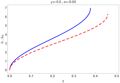
Figure 4: The total angle integrals $I_{F}$ and $I_{FD}$. The solid blue (in color) curve denotes the present approximation of $I_{FD}$ by Eq. (67) and the dashed red (in color) curve denotes numerical calculations of $I_{F}$ in Eq. (19), where we assume the same values for $\kappa$ and $\gamma$ in Figure 3. For the simplicity, we choose $z\equiv z_{R}=z_{S}$, which is denoted by the horizontal axis. For $z\ll 1$, the two curves are very close to each other, because the quadratic approximation works well especially near $z\sim 0$. The two curves are close to each other especially for smaller $z$. For instance, the difference between them is roughly 20 percents at $z\sim 0.2$. A significant deviation at large $z$ reflects a departure from the quadratic approximation of $H(z)$ in $z$.

It is natural that $I_{FR}$ is much smaller than $I_{FD}$, as discussed in Section III. Eq. (67) shows the mild deflection in terms of the arcsine function. See Figure 4 for a comparison of Eq. (67) and numerical calculations for $I_{FD}$. As shown in Figure 3, $f$ are dependent on rather strongly on $\gamma$. The difference between the numerical $f$ and approximate one becomes significant as $z$ is larger. On the other hand, the closest approach and its vicinity make a dominant contribution to the total angle integral $I_{F}$. In Figure 4, therefore, $I_{F}$ shows much weaker dependence on $\gamma$ and $z$.

Finally, we discuss the gap size. By using Eq. (64) for Eq. (50), we obtain

$$\Delta b=\frac{b_{m}^{3}z_{L}^{2}}{8r_{m}^{2}}.$$ (70)

For $b_{m}\sim r_{m}$, furthermore, it becomes simply

$$\Delta b\approx\frac{1}{8}b_{m}z_{L}^{2}.$$ (71)

In a SSS spacetime, the photon sphere was thought to be always an edge such as the inner boundary of a black hole shadow. However, Eqs. (70) and (71) provide a counterexample, when the PS is stable.

V Conclusion

We demonstrated that the location of a stable PS in a compact object is not always an edge such as the inner boundary of a black hole shadow. We showed also that a SSS spacetime cannot be asymptotically flat, when the SOPS exists in the spacetime.

We proved a proposition that the closest approach of a photon is prohibited in the immediate vicinity of the stable PS when the photon is emitted from a source (or reaches a receiver) distant from a lens object. We discussed the gap size. Because of the existence of the gap, the mild deflection is caused for a photon traveling around the stable PS which exists in a class of SSS spacetimes.

Finally, we used a class of SSS solutions in Weyl gravity in order to exemplify the mild deflection near the stable outer PS. It would be interesting to examine whether a light ray is mildly deflected around a stable photon surface in a less symmetric or dynamical spacetime. It is left for future.

- (1) F. W. Dyson, A. S. Eddington, and C. Davidson, Phil. Trans. R. Soc. A 220, 291 (1920).
- (2) K. Akiyama et al. (Event Horizon Telescope Collaboration), Astrophys. J. 875, L1 (2019); Astrophys. J. 875, L2 (2019); Astrophys. J. 875, L3 (2019); Astrophys. J. 875, L4 (2019); Astrophys. J. 875, L5 (2019); Astrophys. J. 875, L6 (2019).
- (3) K. Akiyama et al. (Event Horizon Telescope Collaboration), Astrophys. J. 910, L12 (2021).
- (4) K. Akiyama et al. (Event Horizon Telescope Collaboration), Astrophys. J. 910, L13 (2021).
- (5) C. Darwin, Proc. Roy. Soc. Lond. A 249,180 (1959).
- (6) V. Bozza, Phys. Rev. D 66, 103001 (2002).
- (7) N. Tsukamoto, Phys. Rev. D 95, 064035 (2017).
- (8) N. Tsukamoto, Phys. Rev. D 102, 104029 (2020).
- (9) N. Tsukamoto, Phys. Rev. D 104, 064022 (2021).
- (10) N. Tsukamoto, Phys. Rev. D. 104, 124016 (2021).
- (11) V. Perlick, Living Rev. Relativity 7, 9 (2004).
- (12) N. G. Sanchez, Phys. Rev. D 18, 1030 (1978).
- (13) C. M. Claudel, K. S. Virbhadra, and G. F. R. Ellis, J. Math. Phys. 42, 818 (2001).
- (14) S. Hod, Phys. Lett. B 727, 345 (2013).
- (15) Y. Decanini, A. Folacci, and B. Raffaelli, Phys. Rev. D 81, 104039 (2010).
- (16) S. W. Wei, Y. X. Liu, and H. Guo, Phys. Rev. D 84, 041501(R) (2011).
- (17) I. Z. Stefanov, S. S. Yazadjiev, and G. G. Gyulchev, Phys. Rev. Lett. 104, 251103 (2010).
- (18) M. Cvetic, G. W. Gibbons, and C. N. Pope, Phys. Rev. D 94, 106005 (2016).
- (19) G. W. Gibbons, and C. M. Warnick, Phys. Lett. B 763, 169 (2016).
- (20) T. Ohgami, and N. Sakai, Phys. Rev. D 91, 124020 (2015).
- (21) Y. Koga and T. Harada, Phys. Rev. D 94, 044053 (2016).
- (22) Y. Koga and T. Harada, Phys. Rev. D 98, 024018 (2018).
- (23) Y. Koga, Phys. Rev. D 99, 064034 (2019).
- (24) Y. Koga, Phys. Rev. D 101, 104022 (2020).
- (25) Y. Koga, T. Igata, and K. Nakashi, Phys. Rev. D 103, 044003 (2021).
- (26) T. Shiromizu, Y. Tomikawa, K. Izumi, and H. Yoshino, Prog. Theor. Exp. Phys. 2017, 033E01 (2017).
- (27) H. Yoshino, K. Izumi, T. Shiromizu, and Y. Tomikawa, Prog. Theor. Exp. Phys. 2017, 063E01 (2017).
- (28) H. Yoshino, K. Izumi, T. Shiromizu, and Y. Tomikawa, Prog. Theor. Exp. Phys. 2020, 023E02 (2020).
- (29) H. Yoshino, K. Izumi, T. Shiromizu, and Y. Tomikawa, Prog. Theor. Exp. Phys. 2020, 053E01 (2020).
- (30) R. Yang, and H. Lu, Eur. Phys. J. C 80, 949 (2020).
- (31) K. Izumi, Y. Tomikawa, T. Shiromizu, and H. Yoshino, Prog. Theor. Exp. Phys. 2021, 083E02 (2021).
- (32) C. Cederbaum, and G. J. Galloway, Class. Quantum Grav. 33, 075006 (2016).
- (33) A. K. Mishra, S. Chakraborty, and S. Sarkar, Phys. Rev. D 99, 104080 (2019).
- (34) C. Cederbaum, and G. J. Galloway, J. Math. Phys. 62, 032504 (2021).
- (35) M. Guo, and S. Gao, Phys. Rev. D 103, 104031 (2021).
- (36) R. A. Konoplya, and A. Zhidenko, Phys. Rev. D 103, 104033 (2021).
- (37) Q. Gan, P. Wang, H. Wu, and H. Yang, Phys. Rev. D 104, 024003 (2021).
- (38) R. Ghosh, and S. Sarkar, Phys. Rev. D 104, 044019 (2021).
- (39) M. Siino, Class. Quantum Grav. 38, 025005 (2021).
- (40) M. Siino, ArXiv:2107.06551.
- (41) K. Takizawa, and H. Asada, Phys. Rev. D 103, 104039 (2021).
- (42) V. Bozza, Phys. Rev. D 78, 103005 (2008).
- (43) K. Takizawa, T. Ono, and H. Asada, Phys. Rev. D 101, 104032 (2020).
- (44) K. Takizawa, T. Ono, and H. Asada, Phys. Rev. D 102, 064060 (2020).
- (45) P. V. P. Cunha, E. Berti and C. A. R. Herdeiro, Phys. Rev. Lett. 119, 251102 (2017).
- (46) S. Hod, Phys. Lett. B 776, 1 (2018).
- (47) W. Hasse and V. Perlick, Gen. Rel. Grav. 34, 415, (2002).
- (48) A. Ishihara, Y. Suzuki, T. Ono, T. Kitamura and H. Asada, Phys. Rev. D 94, 084015 (2016).
- (49) A. Ishihara, Y. Suzuki, T. Ono and H. Asada, Phys. Rev. D 95, 044017 (2017).
- (50) T. Ono, A. Ishihara, and H. Asada, Phys. Rev. D 96, 104037 (2017).
- (51) T. Ono, and H. Asada, Universe, 5(11), 218 (2019).
- (52) V. Cardoso, L. C. B. Crispino, C. F. B. Macedo, H. Okawa, and P. Pani, Phys. Rev. D 90, 044069 (2014).
- (53) J. Keir, Class. Quantum Grav. 33, 135009 (2016).
- (54) A. Addazi, A. Marciano, and N. Yunes, Eur. Phys. J. C 80, 36 (2020).
- (55) T. Chiba, and M. Kimura, Prog. Theor. Exp. Phys. 4, 043E01 (2017).
- (56) There is a prohibited region around the stable PS as shown in Section IIID. Because the existence of this gap region, the functions and are not differentiable at . As a result, and cannot be Taylor-expanded around . In stead of Taylor expansions, therefore, we look for asymptotic expansions of , and through , and .
- (57) P. D. Mannheim, and D. Kazanas, Astrophys. J. 342, 635 (1989).
- (58) Turner and Horne realized that a bound orbit of a photon is possible in this parameter region for the SSS solution in Weyl gravity TH .
- (59) G. E. Turner, and K. Horne, Class. Quantum Grav. 37, 095012 (2020).