Bayesian inference and Markov chain Monte Carlo based estimation of a geoscience model parameter

Abstract

The critical slip distance in rate and state model for fault friction in the study of potential earthquakes can vary wildly from micrometers to few meters depending on the length scale of the critically stressed fault. This makes it incredibly important to construct an inversion framework that provides good estimates of the critical slip distance purely based on the observed acceleration at the seismogram. The framework is based on Bayesian inference and Markov chain Monte Carlo. The synthetic data is generated by adding noise to the acceleration output of spring-slider-damper idealization of the rate and state model as the forward model.

backgroundcolor=, commentstyle=, keywordstyle=, numberstyle=, stringstyle=, basicstyle=, breakatwhitespace=false, breaklines=true, captionpos=b, keepspaces=true, numbers=left, numbersep=5pt, showspaces=false, showstringspaces=false, showtabs=false, tabsize=2

[inst1]organization=University of Southern California,city=Los Angeles, postcode=90007, state=CA, country=USA

[inst2]organization=North Carolina State University,city=Raleigh, postcode=27607, state=NC, country=USA

1 Introduction

The quantification of fault slip is achieved using the Rate- and State-dependent Friction (RSF) model for friction evolution, which is considered the gold standard for modeling earthquake cycles on faults [1, 2, 3, 4, 5, 6]. It is given by

$$\left.\begin{array}[]{c}\mu=\mu_{0}+A\ln{\left(\frac{V}{V_{0}}\right)}+B\ln{\left(\frac{V_{0}\theta}{d_{c}}\right)},\\ \frac{d\theta}{dt}=1-\frac{\theta V}{d_{c}},\end{array}\right.$$ (3)

where $V=|d\boldsymbol{d}/dt|$ is the slip rate magnitude, $a=\frac{dV}{dt}$ which we hypothesize is of the same order as recorded by seismograph, $\mu_{0}$ is the steady-state friction coefficient at the reference slip rate $V_{0}$, $A$ and $B$ are empirical dimensionless constants, $\theta$ is the macroscopic variable characterizing state of the surface and $d_{c}$ is a critical slip distance. The critical slip distance is the distance over which a fault loses or regains its frictional strength after a perturbation in the loading conditions [7]. In principle, it determines the maximum slip acceleration and radiated energy to such an extent that it influences the magnitude and time scale of the associated stress breakdown process [8]. Regardless of the importance, it is paradoxical that the values of $d_{c}$ reported in the literature range from a few to tens of microns as determined in typical laboratory experiments [8], to $0.1-5\,m$ as determined in numerical and seismological estimates based on geophysical observations [9], and further to several meters as determined in high‐velocity laboratory experiments [10]. Moreover, in most numerical simulations of dynamic rupture propagation with prescribed friction laws, $d_{c}$ is imposed a priori and its value is often assumed to be constant and uniform on the fault plane. Understanding the physics that controls the critical slip distance and explains the gap between observations from experimental and natural faults is thus one of the crucial problems in both the seismology and laboratory communities [11].

With that in mind, we provide a framework in which synthetic earthquake data is used to quantify uncertainty in critical slip distance. While the resolution and coupled flow and poromechanics [12, 13, 14, 15, 16, 17, 18, 19, 20, 21, 22, 23, 24] associated with subsurface activity in the realm of energy technologies and concomitant earthquake quantification is a hot topic, in this work, we focus on the effect of a standard trigonometric perturbation with exponentially decreasing amplitude. In section 2, we explain the spring slider damper idealization to infer the influence of critical slip distance on RSF without recourse to complicated elastodynamic equations. In section 3, we explain the Bayesian inference framework to inversely quantify uncertainty in the estimation of critical slip distance. In section 4, we present the results from our investigation. In section 5, we present conclusions and outlook for future work.

2 The forward model

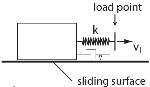
Figure 1: Spring Slider Damper Idealization of Fault Behavior

As shown in Fig. 1, we model a fault by a slider spring system [25, 26, 27]. The slider represents either a fault or a part of the fault that is sliding. The stiffness $k$ represents elastic interactions between the fault patch and the ductile deeper part of the fault, which is assumed to creep at a constant rate. This simple model assumes that slip, stress, and friction law parameters are uniform on the fault patch. The friction coefficient of the block is given by

$$\mu=\frac{\tau}{\sigma}=\frac{\tau_{l}-k\delta-\eta V}{\sigma}$$

where $\sigma$ is the normal stress, $\tau$ the shear stress on the interface, $\tau_{l}$ is the remotely applied stress acting on the fault in the absence of slip, -$k\delta$ is the decrease in stress due to fault slip [28] and $\eta$ is the radiation damping coefficient [29]. We consider the case of a constant stressing rate $\dot{\tau_{l}}=kV_{l}$ where $V_{l}$ is the load point velocity, which we take to be

$$V_{l}=V_{0}(1+\exp{(-t/10)}\,sin(10t))$$ (4)

The stiffness is a function of the fault length $l$ and elastic modulus $E$ as $k\approx\frac{E}{l}$. With $k^{\prime}=\frac{E}{l\sigma}$, we get

$$\dot{\mu}\approx k^{\prime}(V_{l}-V)-k^{\prime\prime}\dot{V}$$ (5)

where $k^{\prime\prime}=\frac{\eta}{\sigma}$. Once the phenomenological form of $\dot{\mu}$ is known, we rewrite Eq. (3) as

$$\left.\begin{array}[]{c}V=V_{0}\exp\left(\frac{1}{A}\left(\mu-\mu_{0}-B\ln{\left(\frac{V_{0}\theta}{d_{c}}\right)}\right)\right),\\ \dot{\theta}=1-\frac{\theta V}{d_{c}},\\ \dot{V}=\frac{V}{A}\left(\dot{\mu}-\frac{B}{\theta}\dot{\theta}\right)\end{array}\right.$$ (6)

The ballpark values are:

• Elastic modulus $E=5\times 10^{10}\,Pa$

• Critical fault length $l=3\times 10^{-2}\,m$

• Normal stress $\sigma=200\times 10^{6}Pa$

• Radiation damping coefficient $\eta=20\times 10^{6}Pa/(m/s)$

• $A=0.011$

• $B=0.014$

• $V_{0}=1\mu m/s$

• $\theta_{0}=0.6$

• $\mu_{0}=\mu_{0}=0.6$

from which the effective stiffness and damping are obtained as

• $k^{\prime}=\frac{E}{l\sigma}=\frac{5\times 10^{10}}{3\times 10^{-2}\times 2\times 10^{8}}[1/m]\approx 10^{-2}[1/\mu m]$

• $k^{\prime\prime}=\frac{\eta}{\sigma}=\frac{2\times 10^{7}}{2\times 10^{8}}[s/m]=10^{-7}[s/\mu m]$

3 Bayesian inversion framework

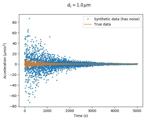
Figure 2: Noise is modeled as normal distribution

To define the inverse problem, considered the relationship between acceleration ($a_{i}(t)$) and the model response by the following statistical model

$$a(t_{i})=f(t_{i},\theta,\mu,A,B,d_{c})+\epsilon_{i}$$ (7)

where $\epsilon_{i}$ is the noise. Assuming the $\epsilon_{i}\sim N(0,\sigma^{2})$ as unbiased, independent and identical normal distribution with standard deviation $\sigma$ allows us to conveniently generate the synthetic data as shown in Fig. 2. The synthetic data over time $a(t_{1}),...,a(t_{n})$ are the $n$ observations for $a(t_{i})$ and $f(A,t_{i},\theta,\mu,A,B,d_{c})$ is the acceleration response of the model over time obtained using the forward model. The goal of the inverse problem is to determine the model parameter ($d_{c}$) from the Eq.(7) . Using the Bayes theorem [30], the distribution for the model parameter is given by the posterior distribution $\pi(d_{c}|a(t_{1}),...,a(t_{n}))$ given by

$$\pi(d_{c}|a(t_{1}),...,a(t_{n}))=\frac{\pi(a(t_{1}),...,a(t_{n})|d_{c})\pi_{0}(d_{c})}{\int_{d_{c}}\pi(a(t_{1}),...,a(t_{n})|d_{c})\pi_{0}(d_{c})dd_{c}}$$ (8)

where $\pi(a(t_{1}),...,a(t_{n})|d_{c})$ is the likelihood given by

$$\pi(a(t_{1}),...,a(t_{n})|d_{c}) =\prod_{i=1}^{n}\pi(a(t_{i})|d_{c})$$

$$=\prod_{i=1}^{n}\frac{1}{\sigma\sqrt{2\pi}}e^{-\frac{1}{2}\left(\frac{a(t_{i})-f(V,t_{i},\theta,\mu,A,B,d_{c})}{\sigma}\right)^{2}}$$ (9)

and $\pi_{0}(d_{c})$ is the prior distribution. The denominator is a normalizing integral. The information of the model parameter can be included in the posterior distribution through the prior, $\pi_{0}(d_{c})$. In this study, the prior is assumed to be uniform distribution and the prior is a constant value inside the uniform distribution limits. The quantity that makes evaluation of the posterior difficult is the integral term in the denominator. Direct evaluation of the integral using quadrature rules is expensive and often requires adaptive methods. Alternatively, sampling methods like Markov chain Monte Carlo (MCMC) methods [31, 32, 33, 34] can be used to evalute the integral.

The MCMC method generates the parameter samples from a proposal distribution, and the sample is rejected or accepted by evaluating the posterior distribution for the corresponding parameter sample. Adaptive Metropolis MCMC algorithm [33] is used as the sampling method. The MCMC simulation starts from a random value for the model parameter generated from uniform bounded distribution. The MCMC sampling method uses the obtained predicted acceleration and a new value for the model parameter is generated using the Markov chain. The errors are assumed to be a normal distribution with a standard deviation and at each iteration of the MCMC sampling method, a new value of standard deviation is generated, associated with the model parameter using inverse-gamma distribution. In the next iteration, the predictive model is solved again for the new parameter and the obtained predicted acceleration is used by the MCMC sampling method to generate the next parameter sample. A total of $n$ MCMC samples are generated from the MCMC sampling method.

4 Results

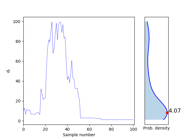
(a) 100 samples

(b) 500 samples

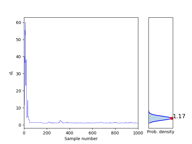
(c) 1000 samples

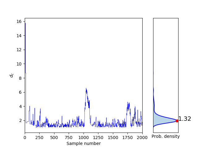
(d) 2000 samples

Figure 3: Output of the Bayesian MCMC framework for model parameter for different sample numbers with true value of $d_{c}=1\,\mu m$ and an initial guess of $10\,\mu m$

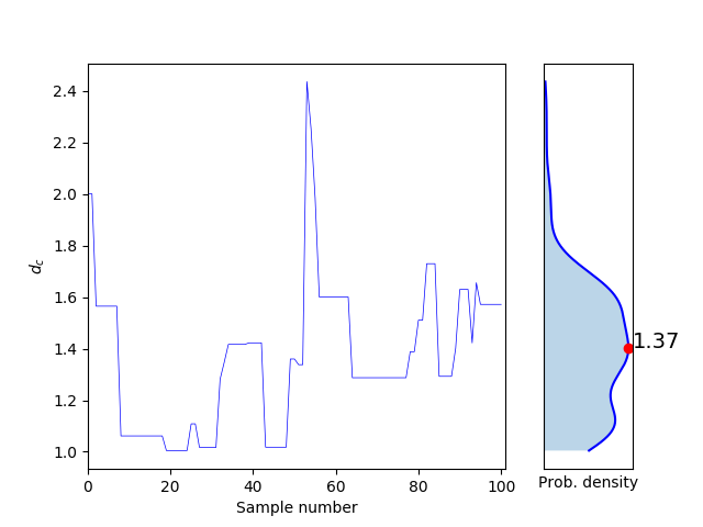
(a) 100 samples

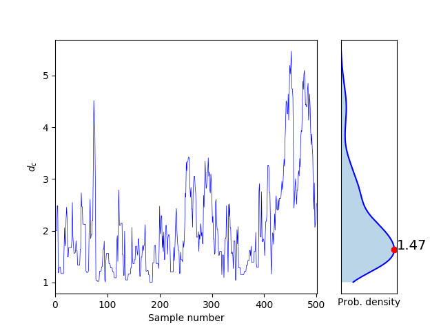
(b) 500 samples

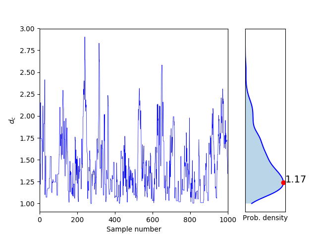
(c) 1000 samples

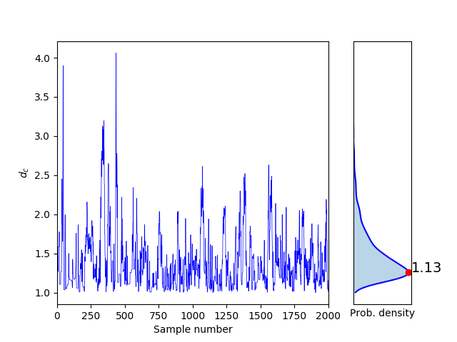
(d) 2000 samples

Figure 4: Output of the Bayesian MCMC framework for model parameter for different sample numbers with true value of $d_{c}=1\,\mu m$ and an initial guess of $2\,\mu m$

Figs. 3- 4 show a gradual improvement in the estimated model parameter as the number of samples is increased. It is evident that the framework has a lot more difficulty converging to the true value if the initial guess is far away from the true value. In reality, it is not really known what the true value is, and arbitrary initial guesses will lend a solution that is way off target regardless of the number of sampling points. We observe that the Bayesian framework settles to a value with maximum probability after a certain number of sampling points regardless of the number of samples following it. In all of the simulations, we observe in all the simulations that the Bayesian framework does an excellent job of dropping to the ballpark of the expected true value within the first few samples. We see that the framework is not heavily reliant on the initial guess for accuracy for the set of simulations we are rendering.

5 Conclusions and Outlook

The rate and state model for fault friction evolution is a piece of the puzzle in which forward simulations are used to arrive at the seismic impact of fault slip on earthquake activity. Typically, the earthquakes are measured with seismograms and geophones on the surface as P-waves and S-waves, and then these readings are used to calibrate the seismic activity for constant monitoring. The acceleration field around the fault slip activity translates to these waves recorded on the surface, and forward simulations with wave propagation bridge that gap. That being said, a seismic recording on the surface cannot easily be backtraced to acceleration around the fault, and finally to the source of the fault slip. That is precisely inverse modeling, and the Bayesian framework coupled with MCMC allows us to put such a framework in place. The accelerations are field quantities, and the inverse estimation of the field around the fault from the time series at the seismogram and/or geophone is not a trivial task. With that in mind, we test the robustness of the Bayesian/MCMC framework to inversely estimate a value instead of a field. The thing is that any inversion framework works on data as the input, and since subsurface data is not available other the sensors at the wells, the forward simulations are used to generate this data with all the computational physics put in place. This generated data is then used to inversely estimate the acceleration field from the data at the surface. Although such forward simulations to generate data are infeasible in real-time scenarios where we need estimates of what is happening in the subsurface from the reading on the surface almost immediately, the framework robustness would eventually lend itself to that scenario. The scenario is that the recording at the seismogram and/or geophone would be fed into the Bayesian/MCMC fraemwork as an input, and the framework would provide an estimate of the acceleration field around the fault as the output. In this work, we work on arriving at estimates of critical slip distance in the rate and state model by running a spring-slider-damper as the forward model instead of using a full-fledged forward simulator. In the future, we will be deploying the coupled flow and geomechanics simulator as the forward model, and gradually arrive at the aforementioned scenario.

References

- [1] A. L. Ruina. Slip instability and state variable friction laws. Geophys. Res. Lett., 88:359–370, 1983.
- [2] C. H. Scholz. Mechanics of faulting. Ann. Rev. Earth Planet. Sci., 17:309–334, 1989.
- [3] C. Marone. Laboratory-derived friction laws and their application to seismic faulting. Ann. Rev. Earth Planet. Sci., 26:643–696, 1998.
- [4] Meng Wei and Pengcheng Shi. Synchronization of earthquake cycles of adjacent segments on oceanic transform faults revealed by numerical simulation in the framework of rate-and-state friction. Journal of Geophysical Research: Solid Earth, 126(1):e2020JB020231, 2021.
- [5] Yunzhong Jia, Jiren Tang, Yiyu Lu, and Zhaohui Lu. The effect of fluid pressure on frictional stability transition from velocity strengthening to velocity weakening and critical slip distance evolution in shale reservoirs. Geomechanics and Geophysics for Geo-Energy and Geo-Resources, 7(1):1–13, 2021.
- [6] Zhu Weiqiang, Kali Allison, Eric Dunham, and Yuyun Yang. Fault valving and pore pressure evolution in simulations of earthquake sequences and aseismic slip. Nature communications, 11:4833, 09 2020.
- [7] Andrew Clennel Palmer and James Robert Rice. The growth of slip surfaces in the progressive failure of over-consolidated clay. Proceedings of the Royal Society of London. A. Mathematical and Physical Sciences, 332(1591):527–548, 1973.
- [8] Christopher H Scholz. The mechanics of earthquakes and faulting. Cambridge university press, 2019.
- [9] Yoshihiro Kaneko, Eiichi Fukuyama, and Ian James Hamling. Slip-weakening distance and energy budget inferred from near-fault ground deformation during the 2016 mw7. 8 kaikōura earthquake. Geophysical Research Letters, 44(10):4765–4773, 2017.
- [10] André Niemeijer, Giulio Di Toro, Stefan Nielsen, and Fabio Di Felice. Frictional melting of gabbro under extreme experimental conditions of normal stress, acceleration, and sliding velocity. Journal of Geophysical Research: Solid Earth, 116(B7), 2011.
- [11] Mitiyasu Ohnaka. A constitutive scaling law and a unified comprehension for frictional slip failure, shear fracture of intact rock, and earthquake rupture. Journal of Geophysical Research: Solid Earth, 108(B2), 2003.
- [12] Saumik Dana and Mary F Wheeler. Augmented lagrangian for treatment of hanging nodes in hexahedral meshes. arXiv preprint arXiv:1809.04031, 2018.
- [13] Saumik Dana and Karthik Reddy Lyathakula. Uncertainty quantification in friction model for earthquakes using bayesian inference. arXiv preprint arXiv:2104.11156, 2021.
- [14] S. Dana and M. F. Wheeler. Convergence analysis of fixed stress split iterative scheme for anisotropic poroelasticity with tensor biot parameter. Computational Geosciences, 22(5):1219–1230, 2018.
- [15] S. Dana and M. F. Wheeler. Convergence analysis of two-grid fixed stress split iterative scheme for coupled flow and deformation in heterogeneous poroelastic media. Computer Methods in Applied Mechanics and Engineering, 341:788–806, 2018.
- [16] Saumik Dana and Mary F Wheeler. Design of convergence criterion for fixed stress split iterative scheme for small strain anisotropic poroelastoplasticity coupled with single phase flow. arXiv preprint arXiv:1912.06476, 2019.
- [17] Saumik Dana and Mary F Wheeler. An efficient algorithm for numerical homogenization of fluid filled porous solids: part-i. arXiv preprint arXiv:2002.03770, 2020.
- [18] Saumik Dana and Mary F Wheeler. A machine learning accelerated fe2 homogenization algorithm for elastic solids. arXiv preprint arXiv:2003.11372, 2020.
- [19] Saumik Dana, Benjamin Ganis, and Mary F. Wheeler. A multiscale fixed stress split iterative scheme for coupled flow and poromechanics in deep subsurface reservoirs. Journal of Computational Physics, 352:1–22, 2018.
- [20] Saumik Dana, Mohamad Jammoul, and Mary F Wheeler. Performance studies of the fixed stress split algorithm for immiscible two-phase flow coupled with linear poromechanics. Computational Geosciences, pages 1–15, 2021.
- [21] Saumik Dana, Joel Ita, and Mary F Wheeler. The correspondence between voigt and reuss bounds and the decoupling constraint in a two-grid staggered algorithm for consolidation in heterogeneous porous media. Multiscale Modeling & Simulation, 18(1):221–239, 2020.
- [22] Saumik Dana. A simple framework for arriving at bounds on effective moduli in heterogeneous anisotropic poroelastic solids. arXiv preprint arXiv:1912.10835, 2019.
- [23] Saumik Dana. System of equations and staggered solution algorithm for immiscible two-phase flow coupled with linear poromechanics. arXiv preprint arXiv:1912.04703, 2019.
- [24] S. Dana. Addressing challenges in modeling of coupled flow and poromechanics in deep subsurface reservoirs. PhD thesis, The University of Texas at Austin, 2018.
- [25] James R Rice and Ji-cheng Gu. Earthquake aftereffects and triggered seismic phenomena. Pure and Applied Geophysics, 121(2):187–219, 1983.
- [26] Ji-Cheng Gu, James R Rice, Andy L Ruina, and T Tse Simon. Slip motion and stability of a single degree of freedom elastic system with rate and state dependent friction. Journal of the Mechanics and Physics of Solids, 32(3):167–196, 1984.
- [27] James H Dieterich. Earthquake nucleation on faults with rate-and state-dependent strength. Tectonophysics, 211(1-4):115–134, 1992.
- [28] Hiroo Kanamori and Emily E Brodsky. The physics of earthquakes. Reports on Progress in Physics, 67(8):1429, 2004.
- [29] Mark W McClure and Roland N Horne. Investigation of injection-induced seismicity using a coupled fluid flow and rate/state friction model. Geophysics, 76(6):WC181–WC198, 2011.
- [30] Ralph C Smith. Uncertainty quantification: theory, implementation, and applications, volume 12. Siam, 2013.
- [31] Alexander Shapiro. Monte carlo sampling methods. Handbooks in operations research and management science, 10:353–425, 2003.
- [32] W Keith Hastings. Monte carlo sampling methods using markov chains and their applications. 1970.
- [33] Heikki Haario, Eero Saksman, and Johanna Tamminen. An adaptive metropolis algorithm. Bernoulli, pages 223–242, 2001.
- [34] Christian Lorenz Mueller. Exploring the common concepts of adaptive mcmc and covariance matrix adaptation schemes. In Dagstuhl Seminar Proceedings. Schloss Dagstuhl-Leibniz-Zentrum fÃr Informatik, 2010.