Free vibrations of axially moving strings: Energy estimates and boundary observability

Abstract.

We study the small vibrations of axially moving strings described by a wave equation in an interval with two endpoints moving in the same direction with a constant speed. The solution is expressed by a series formula where the coefficients are explicitly computed in function of the initial data. We also define an energy expression for the solution that is conserved in time. Then, we establish boundary observability inequalities with explicit constants.

1. Introduction

The present work deals with small transverse vibrations of an infinite string moving axially with a constant speed. Two fixed supports, distanced by $L$ as represented in Figure 1, prevent transversal displacements of the string at the supporting points while the axial motion remains unaffected.

Figure 1. A string travelling to the left with a speed $v$.

We introduce a coordinate system $(x,t)$, attached to the travelling string, where $x$ coincides with the rest state axis of the string and $t$ denotes the time. We denote transverse displacement of the string by $\phi(x,t)$ and we choose the position of the left support to coincide with $x=0$. Assuming that the string travels to the left with a scalar speed $v$, the positions of the left and right supports are $x=vt$ and $x=L+vt$ for $t\geq 0$, respectively. If we assume that the string travels to the right then it suffices to change $v$ by $-v$ in the remainder of this paper.

For $T>0,$ we denote the interval

$$\mathbf{I}_{t}:=\left(vt,L+vt\right),\text{ \ for\ }t\in\left(0,T\right).$$

A simplified model describing the free small transverse vibrations of this string is the following wave equation

$$\left\{\begin{array}[]{ll}\phi_{tt}-\phi_{xx}=0,\ \vskip 3.0pt plus 1.0pt minus 1.0pt&\text{for }x\in\mathbf{I}_{t}\text{ and }t\in\left(0,T\right),\\ \phi\left(vt,t\right)=\phi\left(L+vt,t\right)=0,\vskip 3.0pt plus 1.0pt minus 1.0pt&\text{for }t\in\left(0,T\right),\\ \phi(x,0)=\phi^{0}\left(x\right)\text{, \ \ }\phi_{t}\left(x,0\right)=\phi^{1}\left(x\right),\text{ \ }&\text{for }x\in\mathbf{I}_{0},\end{array}\right.$$ (WP)

where the subscripts $t$ and $x$ stand for the derivatives in time and space variables respectively, $\phi^{0}$ is the initial shape of the string and $\phi^{1}$ is its initial transverse speed. We assume that the speed $v$ is strictly less then the speed of propagation of the wave (here normalized to $c=1$), i.e.

$$0<v<1.$$ (1.1)

If $v\geq 1,$ then the problem is ill-posed, see for instance [1].

The wave equation formulated above is a simple model to represent several mechanical systems such as plastic films, magnetic tapes, elevator cables, textile and fibre winding, see for example [2, 3, 4]. This model can be dated back to Skutch [5], its simplicity is only apparent and we should mention that the method of separation of variables cannot be applied to this problem. Miranker’s work [6] is one of the early influencing papers on the topic of axially moving media. He proposed two approaches to solve Problem (WP). The first one is to ”freeze” the space interval by formulating the problem in the interval $\left(0,L\right)$. Thus, introducing the variables $\eta=x-vt$ and $\tau=t$, the first equation in (WP) becomes

$$\phi_{\tau\tau}-2v\phi_{\eta\tau}-\left(1-v^{2}\right)\phi_{\eta\eta}=0,\text{ \ for }\eta\in\left(0,L\right),\text{ }\tau>0.$$ (1.2)

The obtained problem is more familiar and the vast majority of the literature on travelling strings follows this approach. Some important results in this direction are given by Wickert and Mote [7] where the authors write (1.2) as a first-order differential equation with matrix differential operators (a state space formulation) and obtained a closed form representation of the solution for arbitrary initial conditions. There is also other methods to solve (1.2), for instance a solution by the Laplace transform method is proposed in [8]. The solution can also be constructed using the characteristic method, see for instance [1, 9].

The approach of Miranker [6] is to solve (WP), i.e. keep the space interval depending on time. He obtained a closed form of the solution by a series formulas (See page 39 in [6]). After few rearrangements, his formulas can be rewritten as

$$\phi(x,t)=\sum_{n\in\mathbb{\mathbb{Z}}^{\ast}}c_{n}\left(e^{n\pi i\left(1-v\right)\left(t+x\right)/L}-e^{n\pi i\left(1+v\right)\left(t-x\right)/L}\right),\text{ for }x\in\mathbf{I}_{t}\text{ and }t\in\left(0,T\right).$$ (1.3)

Despite the utility of such a formula for numerical and asymptotic approaches, it remained underexploited in the literature related to axially moving strings.

Since Miranker was not explicit on how to compute the coefficients $c_{n}$, we give in the paper at hands a method to compute each $c_{n}$ in function of the initial data $\phi^{0}\$and $\phi^{1},$ see Theorem 1 in the next section. The idea is inspired from [10] where the second author obtained the exact solution of strings with two linearly moving endpoints at different speeds. Similar techniques were used in [11, 12] for a string with one moving endpoint. Each problem in [10, 11, 12], is set in an interval expanding with time (in the inclusion sense) and the solution is presented by a series containing a type of functions different from those in (1.3). Thus, the results of [10, 12] in particular do not apply to the present problem (WP).

In this work, we show that the series formulas (1.3) can be manipulated to establish the following results:

• A conserved quantity. The functional

  $$\mathcal{E}_{v}\left(t\right)=\frac{1}{2}\int_{vt}^{L+vt}\left(\phi_{t}+v\phi_{x}\right)^{2}+\left(1-v^{2}\right)\phi_{x}^{2}dx,\ \ \ \text{for }t\geq 0,$$ (1.4)

  depending on $L,t,v$ and the solution of $\left(\ref{wave}\right),$ is conserved in time. We give two different proofs for this fact, see Theorem 2. Note that $\phi_{t}+v\phi_{x}=\frac{d}{dt}\left(\phi\left(x+vt,t\right)\right)$ is the total (called also the material) derivative. Under the assumption (1.1), this functional is positive-definite and we will call it the ”energy” of the solution $\phi$. Although there are many expressions of energy for axially moving strings, see for instance [13, 14], we could not find the definition (1.4) in the literature.

• Exact boundary observability.

  • The wave equation (WP) is exactly observable at any endpoint $x=x_{b}+vt,$ where $x_{b}=0$ or $x_{b}=L$. Due to the finite speed of propagation, the time of observability is expected to be positive and depends on the initial length $L$ and the speed $v$. We show that this time is exactly

    $$T_{v}:=2L/(1-v^{2}),$$

    see Theorems 3.

  • If we observe both endpoints, i.e. for $x=vt$ and $x=L+vt,$ the time of observability is reduced to

    $$\tilde{T}_{v}:=L/(1-v),$$

    see Theorem 4.

Although the problem considered here is linear and extensively studied, the application of Fourier series method to establish the above stated results is new to the best of our knowledge. Let us also note that letting $v\rightarrow 0$ in the above results, we recover some known facts for the wave equation in non-travelling intervals [15, 16]. In particular, $\mathcal{E}_{0}\left(t\right)=\frac{1}{2}\int_{0}^{L}\phi_{t}^{2}+\phi_{x}^{2}dx\$is known to be conserved and we get $T_{0}=2L,\tilde{T}_{0}=L$ as sharp values for boundary observability time.

After the present introduction, we derive an expression for the coefficients of the series formula (1.3). In section 3, we show that the energy $\mathcal{E}_{v}$ is conserved in time. The boundary observability results at one endpoint and at both endpoints are addressed in the last section.

2. Computing the coefficients of the series

To simplify some formulas, we introduce the notation

$$\gamma_{v}:=\frac{1+v}{1-v},\text{ \ \ \ \ }L_{1}:=\frac{1-v}{1+v}L\ \ \text{and \ }L_{2}:=\frac{2}{1-v}L$$

since these constants will appear frequently in the sequel. Note that

$$1<\gamma_{v}<+\infty\text{ \ \ and \ \ }0<L_{1}<L<L_{2}/2,\text{ \ for }0<v<1.$$

For every initial data

$$\phi^{0}\in H_{0}^{1}\left(\mathbf{I}_{0}\right),\text{ \ }\phi^{1}\in L^{2}\left(\mathbf{I}_{0}\right),$$ (2.1)

we already know that if (1.1) holds the solution of Problem (WP) exists and satisfies

$$\phi\in C\left([0,T];H_{0}^{1}\left(\mathbf{I}_{t}\right)\right)\text{\ \ \ and \ \ }\phi_{t}\in C\left([0,T];L^{2}\left(\mathbf{I}_{t}\right)\right),$$ (2.2)

see for instance [17, 18]. Moreover, an easy computation shows that the solution $\phi$ given by (1.3) satisfies the periodicity relation

$$\phi(x+vT_{v},t+T_{v})=\phi(x,t),$$ (2.3)

i.e., after a time $T_{v}=2L/\left(1-v^{2}\right)$ the string travels a distance $vT_{v}$ and return to its original form at time $t$.

2.1. Coefficients expressions

Theorem 1.

Under the assumptions (1.1) and (2.1), the solution of Problem (WP) is given by the series (1.3) where the coefficients $c_{n}\in\mathbb{C}$ are given by any of the two following formulas

$$c_{n} =\frac{1}{4n\pi i}\int_{0}^{L_{2}}\left(\tilde{\phi}_{x}^{0}+\tilde{\phi}^{1}\right)e^{-n\pi i\left(1-v\right)x/L}dx,$$ (2.4)

$$=\frac{1}{4n\pi i}\int_{-L_{1}}^{L}\left(\tilde{\phi}_{x}^{0}-\tilde{\phi}^{1}\right)e^{n\pi i\left(1+v\right)x/L}dx\text{, \ \ for }n\in\mathbb{\ \mathbb{Z}}^{\ast},$$ (2.5)

where $\tilde{\phi}_{x}^{0}$ and $\tilde{\phi}^{1}$ are extensions of the initial data $\phi^{0}$and $\phi^{1}$ on the interval $\left(-L_{1},L_{2}\right)$ given below by (2.7) and (2.8) respectively.

Before proceeding to the proof, let us describe how to extend the function $\phi,\$defined only on $\mathbf{I}_{t}=\left(vt,L+vt\right),$ to the intervals $\left(-L_{1}+vt,vt\right)$ and $\left(L+vt,L_{2}+vt\right)$. On one hand, we set

$$\tilde{\phi}(x,t)=\left\{\begin{array}[]{ll}-\phi\left(\gamma_{v}\left(vt-x\right)+vt,t\right),&\text{if }x\in\left(-L_{1}+vt,vt\right),\vskip 3.0pt plus 1.0pt minus 1.0pt\\ \phi\left(x,t\right),&\text{if }x\in\left(vt,L+vt\right),\vskip 3.0pt plus 1.0pt minus 1.0pt\\ -\phi\left(\frac{1}{\gamma_{v}}\left(vt-x\right)+\frac{2L}{1+v}+vt,t\right),\text{ \ \ }&\text{if }x\in\left(L+vt,L_{2}+vt\right).\end{array}\right.$$ (2.6)

The obtained function is well defined since the first variable of $\phi$ remains in the interval $\left(vt,L+vt\right)$. In particular, $\tilde{\phi}(vt,t)=\tilde{\phi}(L+vt,t)=0,\$hence the homogeneous boundary conditions at $x=vt$ and $x=L+vt$ remain satisfied, for every $t\geq 0$.

Figure 2. Example of the extension of an initial data $\phi^{0}$.

Remark 1.

If $v=0$, then $L_{1}=L$ and $L_{2}=2L$. In this case, the functions $\tilde{\phi}$ and $\tilde{\phi}_{t}$ are odd on the intervals $\left(-L,L\right)$ and $\left(0,2L\right)$ with respect to the middle of each interval. The extension $\tilde{\phi}_{x}$ is an even function on these intervals.

Taking the derivative of (2.6) with respect to $x$, we obtain,

$$\tilde{\phi}_{x}(x,t)=\left\{\begin{array}[]{ll}\gamma_{v}\phi_{x}\left(\gamma_{v}\left(vt-x\right)+vt,t\right),&\text{if }x\in\left(-L_{1}+vt,vt\right),\vskip 3.0pt plus 1.0pt minus 1.0pt\\ \phi_{x}\left(x,t\right),&\text{if }x\in\left(vt,L+vt\right),\vskip 3.0pt plus 1.0pt minus 1.0pt\\ \frac{1}{\gamma_{v}}\phi_{x}\left(\frac{1}{\gamma_{v}}\left(vt-x\right)+\frac{2L}{1+v}+vt,t\right),\text{ \ \ \ \ }&\text{if }x\in\left(L+vt,L_{2}+vt\right).\end{array}\right.$$ (2.7)

On the other hand, $\tilde{\phi}_{t}(x,t)$ is extended as follows

$$\tilde{\phi}_{t}(x,t)=\left\{\begin{array}[]{ll}-\gamma_{v}\phi_{t}\left(\gamma_{v}\left(vt-x\right)+vt,t\right),&\text{if }x\in\left(-L_{1}+vt,vt\right),\vskip 3.0pt plus 1.0pt minus 1.0pt\\ \phi_{t}\left(x,t\right),&\text{if }x\in\left(vt,L+vt\right),\vskip 3.0pt plus 1.0pt minus 1.0pt\\ \frac{-1}{\gamma_{v}}\phi_{t}\left(\frac{1}{\gamma_{v}}\left(vt-x\right)+\frac{2L}{1+v}+vt,t\right),\text{ \ \ \ \ }&\text{if }x\in\left(L+vt,L_{2}+vt\right).\end{array}\right.$$ (2.8)

Remark 2.

In Figure 3, let $(x_{1},t_{1})$ be the intersection of the two characteristic starting from the initial endpoints $x=0$ and $x=L$, after one reflection on the boundaries. We can check that, the two backward characteristic lines from $(x_{1},t_{1})$ intersect the $x-$axis precisely at $x=-L_{1}$ and $x=L_{2}$.

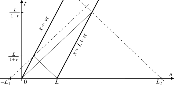
Figure 3. Relation between $L_{1},L_{2}$ and some characteristics of wave propagation.

Now we are ready to show the coefficients formulas.

Proof of Theorem 1.

Thanks to (2.2), we can derive term by term the series (1.3), it comes that

$$\phi_{x}(x,t) =\frac{\pi i}{L}\sum_{n\in\mathbb{\mathbb{Z}}^{\ast}}nc_{n}\left(\left(1-v\right)e^{n\pi i\left(1-v\right)\left(t+x\right)/L}+\left(1+v\right)e^{n\pi i\left(1+v\right)\left(t-x\right)/L}\right),\vskip 3.0pt plus 1.0pt minus 1.0pt$$ (2.9)

$$\phi_{t}(x,t) =\frac{\pi i}{L}\sum_{n\in\mathbb{\mathbb{Z}}^{\ast}}nc_{n}\left(\left(1-v\right)e^{n\pi i\left(1-v\right)\left(t+x\right)/L}-\left(1+v\right)e^{n\pi i\left(1+v\right)\left(t-x\right)/L}\right),$$ (2.10)

where $t\geq 0$, $x\in\left(vt,L+vt\right)$. Combining this, with (2.7) and (2.8), the extensions $\tilde{\phi}_{x}$ and $\tilde{\phi}_{t}$ on the interval $\left(vt,L_{2}+vt\right)$ are given by

$$\tilde{\phi}_{x}(x,t)=\left\{\begin{array}[]{ll}\displaystyle\frac{\pi i}{L}\sum_{n\in\mathbb{\mathbb{Z}}^{\ast}}nc_{n}\left(\left(1-v\right)e^{n\pi i\left(1-v\right)\left(t+x\right)/L}+\left(1+v\right)e^{n\pi i\left(1+v\right)\left(t-x\right)/L}\right),&\text{ if\ }x\in\left(vt,L+vt\right)\vskip 3.0pt plus 1.0pt minus 1.0pt,\\ \displaystyle\frac{\pi i}{\gamma_{v}L}\sum_{n\in\mathbb{\mathbb{Z}}^{\ast}}nc_{n}\left\{\left(1-v\right)e^{\frac{n\pi i\left(1-v\right)}{L}\left(\left(1+v\right)t+\frac{vt-x}{\gamma_{v}}+\frac{2L}{1+v}\right)}\right.,&\\ \lx@intercol\hfil\left.+\left(1+v\right)e^{\frac{n\pi i\left(1+v\right)}{L}\left(\left(1-v\right)t-\frac{vt-x}{\gamma_{v}}-\frac{2L}{1+v}\right)}\right\}\lx@intercol&\lx@intercol\hfil\text{ if\ }x\in\left(L+vt,L_{2}+vt\right),\lx@intercol\end{array}\right.$$ (2.11)

$$\tilde{\phi}_{t}(x,t)=\left\{\begin{array}[]{ll}\displaystyle\frac{\pi i}{L}\sum_{n\in\mathbb{\mathbb{Z}}^{\ast}}nc_{n}\left(\left(1-v\right)e^{n\pi i\left(1-v\right)\left(t+x\right)/L}-\left(1+v\right)e^{n\pi i\left(1+v\right)\left(t-x\right)/L}\right),&\text{ if }x\in\left(vt,L+vt\right)\vskip 3.0pt plus 1.0pt minus 1.0pt,\\ \displaystyle\frac{-\pi i}{\gamma_{v}L}\sum_{n\in\mathbb{\mathbb{Z}}^{\ast}}nc_{n}\left\{\left(1-v\right)e^{\frac{n\pi i\left(1-v\right)}{L}\left(\left(1+v\right)t+\frac{vt-x}{\gamma_{v}}+\frac{2L}{1+v}\right)}\right.,&\\ \lx@intercol\hfil\left.-\left(1+v\right)e^{\frac{n\pi i\left(1+v\right)}{L}\left(\left(1-v\right)t-\frac{vt-x}{\gamma_{v}}-\frac{2L}{1+v}\right)}\right\}\lx@intercol&\lx@intercol\hfil\text{\ if }x\in\left(L+vt,L_{2}+vt\right),\lx@intercol\end{array}\right.$$ (2.12)

Taking the sum of (2.11) and (2.12) on the interval $\left(vt,L_{2}+vt\right)$, we get

$$\tilde{\phi}_{x}+\tilde{\phi}_{t}=\left\{\begin{array}[]{ll}\displaystyle\frac{2\pi i}{L}\left(1-v\right)\sum_{n\in\mathbb{\mathbb{Z}}^{\ast}}nc_{n}e^{n\pi i\left(1-v\right)\left(t+x\right)/L},&x\in\left(vt,L+vt\right),\vskip 6.0pt plus 2.0pt minus 2.0pt\\ \displaystyle\frac{2\pi i}{\gamma_{v}L}\left(1+v\right)\sum_{n\in\mathbb{\mathbb{Z}}^{\ast}}nc_{n}e^{\frac{n\pi i\left(1+v\right)}{L}\left(\left(1-v\right)t-\frac{vt-x}{\gamma_{v}}-\frac{2L}{1+v}\right)},&x\in\left(L+vt,L_{2}+vt\right).\end{array}\right.$$

Since $e^{\frac{n\pi i\left(1+v\right)}{L}\left(\left(1-v\right)t-\frac{vt-x}{\gamma_{v}}-\frac{2L}{1+v}\right)}=e^{n\pi i\left(1-v\right)\left(t+x\right)/L}$, we get the same expression on the two sub-intervals, i.e.

$$\tilde{\phi}_{x}+\tilde{\phi}_{t}=\frac{2\pi i}{L}\left(1-v\right)\sum_{n\in\mathbb{\mathbb{Z}}^{\ast}}nc_{n}e^{n\pi i\left(1-v\right)\left(t+x\right)/L},\text{ \ \ for}\ \ x\in\left(vt,L_{2}+vt\right).$$ (2.13)

Taking into account that $\left\{\sqrt{\frac{1-v}{2L}}e^{n\pi i\left(1-v\right)\left(t+x\right)/L}\right\}_{n\in\mathbb{\mathbb{Z}}}$ is an orthonormal basis for $L^{2}\left(vt,L_{2}+vt\right)$, for every $t\geq 0$, we rewrite (2.13) as

$$\frac{1}{4\pi i}\sqrt{\frac{2L}{1-v}}\left(\tilde{\phi}_{x}+\tilde{\phi}_{t}\right)=\sum_{n\in\mathbb{\mathbb{Z}}^{\ast}}nc_{n}\sqrt{\frac{1-v}{2L}}e^{n\pi i\left(1-v\right)\left(t+x\right)/L},$$ (2.14)

for $x\in\left(vt,L_{2}+vt\right)$. This means that $nc_{n}$ is the $n^{th}$ coefficient of the function

$$\frac{1}{4\pi i}\sqrt{\frac{2L}{1-v}}\left(\tilde{\phi}_{x}+\tilde{\phi}_{t}\right)\in L^{2}\left(vt,L_{2}+vt\right).$$ (2.15)

By consequence,

$$nc_{n}=\frac{1}{4\pi i}\int_{vt}^{L_{2}+vt}\left(\tilde{\phi}_{x}+\tilde{\phi}_{t}\right)e^{-n\pi i\left(1-v\right)\left(t+x\right)/L}dx\text{, \ \ \ for\ }n\in\mathbb{\mathbb{Z}}^{\ast}$$ (2.16)

and (2.4) holds as claimed for $t=0$.

The same argument can be carried out on the interval $\left(-L_{1}+vt,L+vt\right)$ by taking this time the difference between (2.11) and (2.12), we obtain

$$\tilde{\phi}_{x}-\tilde{\phi}_{t}=\left\{\begin{array}[]{ll}\frac{2\pi i}{L}\gamma_{v}\left(1-v\right)\displaystyle\sum_{n\in\mathbb{\ \mathbb{Z}}^{\ast}}nc_{n}e^{n\pi i\left(1-v\right)\left(\left(1+v\right)t+\gamma_{v}\left(vt-x\right)\right)/L},&x\in\left(-L_{1}+vt,vt\right),\vskip 3.0pt plus 1.0pt minus 1.0pt\\ \frac{2\pi i}{L}\left(1+v\right)\displaystyle\sum_{n\in\mathbb{\mathbb{Z}}^{\ast}}nc_{n}e^{n\pi i\left(1+v\right)\left(t-x\right)/L},&x\in\left(vt,L+vt\right).\end{array}\right.$$

After few rearrangement, it follows that

$$\tilde{\phi}_{x}-\tilde{\phi}_{t}=\frac{2\pi i}{L}\left(1+v\right)\sum_{n\in\mathbb{\mathbb{Z}}^{\ast}}nc_{n}e^{n\pi i\left(1+v\right)\left(t-x\right)/L},\text{ \ \ for\ }x\in\left(-L_{1}+vt,L+vt\right).$$ (2.17)

Since $\left\{\sqrt{\frac{1+v}{2L}}e^{n\pi i\left(1+v\right)\left(t-x\right)/L}\right\}_{n\in\mathbb{\mathbb{Z}}}$ is an orthonormal basis for $L^{2}\left(-L_{1}+vt,L+vt\right)$, we deduce that

$$nc_{n}=\frac{1}{4\pi i}\int_{-L_{1}+vt}^{L+vt}\left(\tilde{\phi}_{x}-\tilde{\phi}_{t}\right)e^{-n\pi i\left(1+v\right)\left(t-x\right)/L}dx\text{, \ \ \ for\ }n\in\mathbb{\mathbb{Z}}^{\ast}.$$ (2.18)

For $t=0$, we obtain (2.5) and the theorem follows. ∎

As a byproduct of the above proof, we have the following.

Corollary 1.

Under the assumptions (1.1) and (2.1), the sum $\sum_{n\in\mathbb{\mathbb{Z}}^{\ast}}\left|nc_{n}\right|^{2}$ is finite and is given by any of the two formulas, for $t\geq 0,$

$$\sum_{n\in\mathbb{\mathbb{Z}}^{\ast}}\left|nc_{n}\right|^{2} =\frac{L}{8\pi^{2}\left(1-v\right)}\int_{vt}^{L_{2}+vt}\left(\tilde{\phi}_{x}+\tilde{\phi}_{t}\right)^{2}dx$$ (2.19)

$$=\frac{L}{8\pi^{2}\left(1+v\right)}\int_{-L_{1}+vt}^{L+vt}\left(\tilde{\phi}_{x}-\tilde{\phi}_{t}\right)^{2}dx.$$ (2.20)

Proof.

Parseval’s equality applied to the function given in (2.14) yields

$$\sum_{n\in\mathbb{\mathbb{Z}}^{\ast}}\left|nc_{n}\right|^{2}=\left|\frac{1}{4\pi i}\sqrt{\frac{2L}{1-v}}\right|^{2}\int_{vt}^{L_{2}+vt}\left(\tilde{\phi}_{x}+\tilde{\phi}_{t}\right)^{2}dx\text{, \ \ \ for\ }t\geq 0.$$

Thus (2.19) holds as claimed. The identity (2.20) follows from (2.18) in a similar manner. ∎

2.2. A numerical example

To illustrate the above results, we compute the solution of (WP) for two values of speed $v=0.3$, $v=0.7$ and

$$L=\pi\ ,\phi^{0}\left(x\right)=\sin\left(x\right)/10,\ \ \phi^{1}\left(x\right)=0$$

and use (2.19) for the first 40 frequencies, i.e. $\left|n\right|\leq 40$ in the series sum (1.3). See Figures 4 and 5.

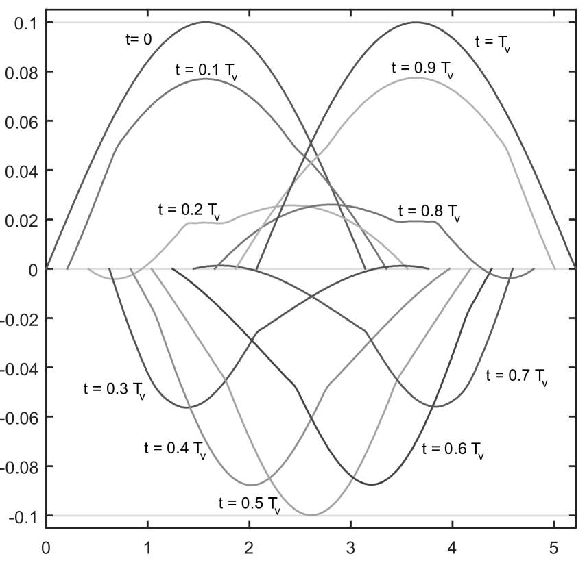
Figure 4. The solution $\phi$ for $v=0.3$ in the interval $(vt,\pi+vt)$ over one period $T_{v}\simeq 6.91$.

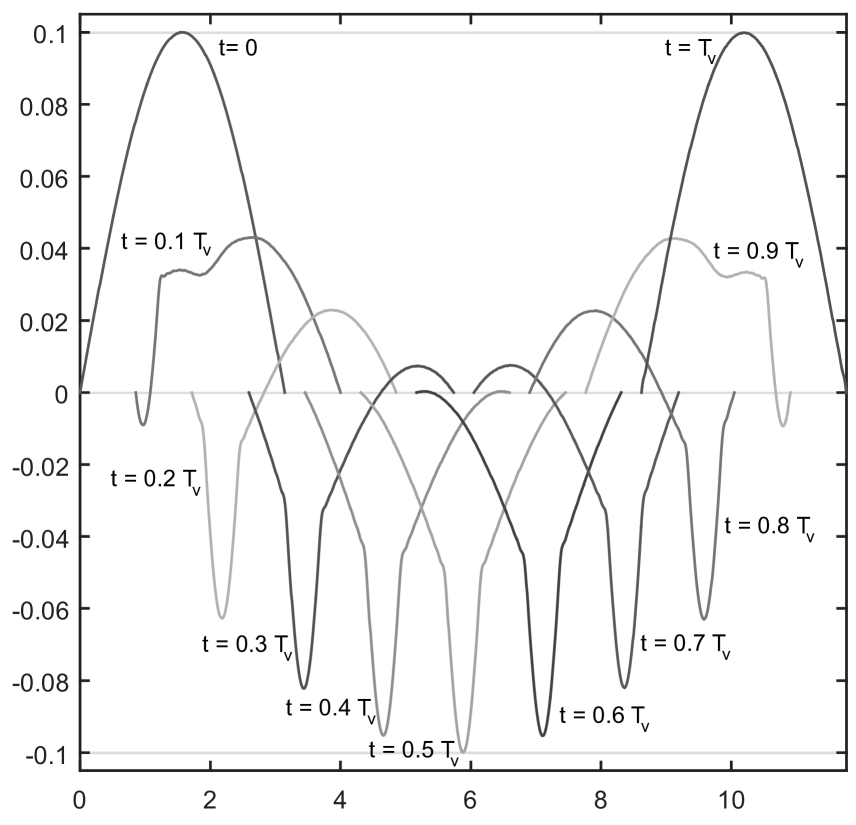
Figure 5. The solution $\phi$ for $v=0.7$ in the interval $(vt,\pi+vt)$ over one period $T_{v}\simeq 12.32$.

3. Energy expressions and estimates

In this section, we show that the energy $\mathcal{E}_{v}\left(t\right)$ of the solution of Problem (WP) is conserved in time.

Theorem 2.

Under the assumptions (1.1) and (2.1), the solution of Problem (WP) satisfies

$$\mathcal{E}_{v}\left(t\right)=\frac{2\pi^{2}\left(1-v^{2}\right)}{L}\sum_{n\in\mathbb{\mathbb{Z}}^{\ast}}\left|nc_{n}\right|^{2},\ \ \ \ \ \text{for}\ t\geq 0.$$ (3.1)

$($the left-hand side is independent of $t).$

Proof.

The two identities (2.19) and (2.20) implies that

$$\frac{1}{1+v}\int_{-L_{1}+vt}^{L+vt}\left(\tilde{\phi}_{x}-\tilde{\phi}_{t}\right)^{2}dx=\frac{1}{1-v}\int_{vt}^{L_{2}+vt}\left(\tilde{\phi}_{x}+\tilde{\phi}_{t}\right)^{2}dx=\frac{8\pi^{2}}{L}\sum_{n\in\mathbb{\ \mathbb{Z}}^{\ast}}\left|nc_{n}\right|^{2}.$$ (3.2)

Using the extensions (2.7), (2.8) and considering the change of variable $x=\frac{1}{\gamma_{v}}\left(vt-\xi\right)+vt$, in $\left(-L_{1}+vt,vt\right),$ we obtain

$$\frac{1}{1+v}\int_{-L_{1}+vt}^{vt}\left(\tilde{\phi}_{x}\left(x,t\right)-\tilde{\phi}_{t}\left(x,t\right)\right)^{2}dx=-\frac{1}{1+v}\int_{L+vt}^{vt}\gamma_{v}\left(\phi_{x}\left(\xi,t\right)+\phi_{t}\left(\xi,t\right)\right)^{2}d\xi\\ =\frac{1}{1-v}\int_{vt}^{L+vt}\left(\phi_{x}\left(\xi,t\right)+\phi_{t}\left(\xi,t\right)\right)^{2}d\xi.$$

Taking $x=\gamma_{v}\left(vt-\xi\right)+\frac{2L}{v-1}+vt$, in $\left(L+vt,L_{2}+vt\right),$ we obtain

$$\frac{1}{1-v}\int_{L+vt}^{L_{2}+vt}\left(\tilde{\phi}_{x}\left(x,t\right)+\tilde{\phi}_{t}\left(x,t\right)\right)^{2}dx=\frac{1}{1+v}\int_{vt}^{L+vt}\left(\phi_{x}\left(\xi,t\right)-\phi_{t}\left(\xi,t\right)\right)^{2}d\xi.$$

Then, taking (3.2) into account, it comes that

$$\frac{1}{1-v}\int_{-L_{1}+vt}^{L+vt}\left(\tilde{\phi}_{t}+\tilde{\phi}_{x}\right)^{2}dx+\frac{1}{1+v}\int_{vt}^{L_{2}+vt}\left(\tilde{\phi}_{x}-\tilde{\phi}_{t}\right)^{2}dx\\ =\frac{2}{1+v}\int_{vt}^{L+vt}\left(\phi_{x}-\phi_{t}\right)^{2}dx+\frac{2}{1-v}\int_{vt}^{L+vt}\left(\phi_{t}+\phi_{x}\right)^{2}dx=\frac{16\pi^{2}}{L}\sum_{n\in\mathbb{\mathbb{Z}}^{\ast}}\left|nc_{n}\right|^{2}.$$

Expanding $\left(\phi_{x}\pm\phi_{t}\right)^{2}$ and collecting similar terms, we get

$$\frac{1}{1-v^{2}}\left(2\int_{vt}^{L+vt}\phi_{x}^{2}+\phi_{t}^{2}+4v\phi_{x}\phi_{t}dx\right)=\frac{8\pi^{2}}{L}\sum_{n\in\mathbb{\mathbb{Z}}^{\ast}}\left|nc_{n}\right|^{2},\text{ \ \ for}\ t\geq 0.$$ (3.3)

Recalling that $\mathcal{E}_{v}\left(t\right)$ is given by (1.4), this identity can be rewritten as in (3.1). This end the proof. ∎

The fact that $\mathcal{E}_{v}\left(t\right)$ is constant in time can be established by using only the identities $\phi_{tt}=\phi_{xx}$ and $\phi\left(vt,t\right)=\phi\left(L+vt,t\right)=0$ from (WP).

A second proof for the conservation of $\mathcal{E}_{v}\left(t\right)$.

It suffices to show that $\frac{d}{dt}\mathcal{E}_{v}\left(t\right)=0.$ First, the boundary conditions $\phi\left(vt,t\right)=\phi\left(L+vt,t\right)=0$ means that $\frac{d}{dt}\phi\left(vt,t\right)=\frac{d}{dt}\phi\left(L+vt,t\right)=0,$ hence

$$\phi_{t}\left(vt,t\right)+v\phi_{x}\left(vt,t\right)=\phi_{t}\left(L+vt,t\right)+v\phi_{x}\left(L+vt,t\right)=0.$$ (3.4)

Since the limits of the integral in the expression of $\mathcal{E}_{v}\left(t\right)$ are time-dependent, then Leibnitz’s rule implies that

$$\frac{d}{dt}\mathcal{E}_{v}\left(t\right)=v\left(1-v^{2}\right)\left(\phi_{x}^{2}\left(L+vt,t\right)-\phi_{x}^{2}\left(vt,t\right)\right)\\ +\int_{vt}^{L+vt}\frac{\partial}{\partial t}\left(\phi_{t}+v\phi_{x}\right)^{2}\ dx+\left(1-v^{2}\right)\frac{\partial}{\partial t}\left(\phi_{x}^{2}\right)dx.$$ (3.5)

The remaining integral equals, after using $\phi_{tt}=\phi_{xx}\$then integrating by parts,

$$\int_{vt}^{L+vt}\left(\phi_{t}+v\phi_{x}\right)\phi_{xx}+\left(v\phi_{t}+\phi_{x}\right)\phi_{xt}dx=\int_{vt}^{L+vt}-\left(\phi_{xt}+v\phi_{xx}\right)\phi_{x}+\left(v\phi_{t}+\phi_{x}\right)\phi_{xt}dx\\ =v\int_{vt}^{L+vt}-\phi_{xx}\phi_{x}+\phi_{t}\phi_{xt}dx,$$

which is nothing but

$$v\int_{vt}^{L+vt}\frac{\partial}{\partial x}\left(\phi_{t}^{2}-\phi_{x}^{2}\right)dx=-v\left(1-v^{2}\right)\left(\phi_{x}^{2}\left(L+vt,t\right)-\phi_{x}^{2}\left(vt,t\right)\right)$$

due to (3.4). Going back to (3.5), we infer that $\frac{d}{dt}\mathcal{E}_{v}\left(t\right)=0$ as claimed. ∎

Let us now compare $\mathcal{E}_{v}\left(t\right)$ to the usual expression of energy for the wave equation

$$E_{v}\left(t\right):=\frac{1}{2}\int_{vt}^{L+vt}\phi_{t}^{2}+\phi_{x}^{2}dx,\text{ \ for}\ t\geq 0.$$

In contrast with $\mathcal{E}_{v}\left(t\right),$ the expression $E_{v}\left(t\right)$ is not conserved in general. Due to the periodicity relation (2.3), we know at least that $E_{v}$ is $T_{v}-$periodic in time. Moreover we have

Corollary 2.

Under the assumptions (1.1) and (2.1), the energy $E_{v}\left(t\right)$ of the solution of Problem (WP) satisfies

$$\frac{\mathcal{E}_{v}\left(t\right)}{1+v}\leq E_{v}\left(t\right)\leq\frac{\mathcal{E}_{v}\left(t\right)}{1-v},\ \ \ \ \ \text{for}\ t\geq 0$$ (3.6)

and

$$\frac{1}{\gamma_{v}}E_{v}\left(0\right)\leq E_{v}\left(t\right)\leq\gamma_{v}E_{v}\left(0\right),\ \ \ \ \ \text{\ for }t\geq 0.$$ (3.7)

Proof.

We can write (3.3) as

$$E_{v}\left(t\right)+v\int_{vt}^{L+vt}\phi_{x}\phi_{t}\ dx=\mathcal{E}_{v}\left(t\right),\text{ \ \ for}\ t\geq 0.$$ (3.8)

Thanks to the algebraic inequality $\pm ab\leq\left(a^{2}+b^{2}\right)/2$ we know that

$$\pm\int_{vt}^{L+vt}\phi_{x}\phi_{t}\ dx\leq E_{v}\left(t\right)\text{, \ \ \ for }t\geq 0.$$

Then, it comes that

$$\mathcal{E}_{v}\left(t\right)\leq\left(1+v\right)E_{v}\left(t\right)\text{ \ \ and \ \ }\left(1-v\right)E_{v}\left(t\right)\leq\mathcal{E}_{v}\left(t\right),\text{ \ for }t\geq 0.$$ (3.9)

This implies (3.6). Since (3.9) holds also for $t=0$, then (3.7) follows by combining the two inequalities

$$\left(1-v\right)E_{v}\left(t\right) \leq\mathcal{E}_{v}\left(t\right)=\mathcal{E}_{v}\left(0\right)\leq\left(1+v\right)E_{v}\left(0\right),$$

$$\left(1-v\right)E_{v}\left(0\right) \leq\mathcal{E}_{v}\left(0\right)=\mathcal{E}_{v}\left(t\right)\leq\left(1+v\right)E_{v}\left(t\right),$$

for $t\geq 0$. ∎

Remark 3.

The equality in estimation (3.6) may hold for some $t\geq 0$. This is the case whenever $\phi_{t}\left(x,t\right)=\pm\phi_{x}\left(x,t\right)$, for $x\in\mathbf{I}_{t}$ and some $t\geq 0$. For instance, if the initial data satisfy $\phi^{1}=\pm\phi_{x}^{0}$ we obtain from (3.8) that

$$\left(1\pm v\right)E_{v}\left(0\right)=E_{v}\left(0\right)+v\int_{0}^{L}\phi_{x}^{0}\phi^{1}\ dx=\mathcal{E}_{v}\left(0\right),$$

i.e. $E_{v}\left(0\right)=\mathcal{E}_{v}\left(0\right)/\left(1\pm v\right)$. By periodicity, we have also $E_{v}\left(nT_{v}\right)=\mathcal{E}_{v}\left(0\right)/\left(1\pm v\right),$ for $n\in\mathbb{Z}$. The + and – signs are used respectively.

Remark 4.

As $v\rightarrow 1^{-},$ we have $\mathcal{E}_{v}\left(0\right)\rightarrow\left\|\phi^{1}+\phi_{x}^{0}\right\|_{L^{2}\left(0,L\right)}/2.$ If the initial data satisfies $\phi^{1}+\phi_{x}^{0}\neq 0,$ it follows from (3.6) that

$$E_{v}\left(t\right)\leq\frac{\mathcal{E}_{v}\left(t\right)}{1-v}=\frac{\mathcal{E}_{v}\left(0\right)}{1-v}\rightarrow+\infty\text{, \ as }v\rightarrow 1^{-}.$$

Taking the precedent remark into account, we may have large value for $E_{v}\left(t\right)$, as $v$ becomes close to the speed of propagation $c=1$, even for small initial value $\mathcal{E}_{v}\left(0\right)$. To see what happens to the string in this case, let us take $v=0.9$ in the precedent numerical example, see Figure 6. We observe a layer effect (i.e. a subregion in $\mathbf{I}_{t}$ where $\phi_{x}$ becomes very large) that travels from the left endpoint to the right one over one period $T_{v}$. This phenomenon becomes more marked as $v$ is closer to $1$.

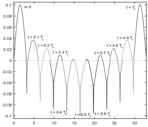
Figure 6. The solution $\phi$ for $v=0.9$ in the interval $(vt,\pi+vt)$ over one period $T_{v}\simeq 33.07$.

4. Boundary observability

In many applications, it is preferred that the sensors do not interfere with the vibrations of the string, so they are placed at the extremities. In addition, interior pointwise sensors are difficult to design and the system may become unobservable depending on the sensors location. This fact was shown by Yang and Mote in [19] where they cast $\left(\ref{freez}\right)$ in a state space form and use semi-group theory.

4.1. Observability at one endpoint

First, we show the observability of (WP) at each endpoint $x_{b}+vt$ where

$$x_{b}=0\ \ \text{or \ }x_{b}=L.$$

The problem of observability considered here can be stated as follows: To give sufficient conditions on the length $T$ of the time interval such that there exists a constant $C(T)>0$ for which the observability inequality

$$\mathcal{E}_{v}\left(0\right)\leq C(T)\int_{0}^{T}\phi_{x}^{2}(x_{b}+vt,t)dt,$$ (4.1)

holds for all the solutions of (WP). This inequality is also called the inverse inequality.

The next theorem shows in particular that the boundary observability holds for $T\geq T_{v}=2L/\left(1-v^{2}\right)$.

Theorem 3.

Under the assumptions (1.1) and (2.1), we have:

$$\int_{0}^{MT_{v}}\phi_{x}^{2}(x_{b}+vt,t)dt=\frac{4M}{\left(1-v^{2}\right)^{2}}\mathcal{E}_{v}\left(0\right).$$ (4.2)

By consequence, the solution of (WP) satisfies the direct inequality

$$\int_{0}^{T}\phi_{x}^{2}(x_{b}+vt,t)dt\leq K_{1}(v,T)\mathcal{E}_{v}\left(0\right)\text{, for every }T\geq 0,$$ (4.3)

with a constant $K_{1}(v,T)$ depending only on $v$ and $T$.

If $T\geq T_{v}$, Problem (WP) is observable at $\xi\left(t\right)=x_{b}+vt$ and it holds that:

$$\mathcal{E}_{v}\left(0\right)\leq\frac{\left(1-v^{2}\right)^{2}}{4}\int_{0}^{T}\phi_{x}^{2}(x_{b}+vt,t)dt.$$ (4.4)

Proof.

Thanks to (2.9), we can evaluate $\phi_{x}$ at the endpoint $x=x_{b}+vt$ . We obtain

$$\phi_{x}(x_{b}+vt,t) =\frac{\pi i}{L}\sum_{n\in\mathbb{\mathbb{Z}}^{\ast}}nc_{n}\left(\left(1-v\right)e^{\frac{n\pi i\left(1-v\right)}{L}\left(\left(1+v\right)t+x_{b}\right)}+\left(1+v\right)e^{\frac{n\pi i\left(1+v\right)}{L}\left(\left(1-v\right)t-x_{b}\right)}\right)$$

$$=\frac{\pi i}{L}\sum_{n\in\mathbb{\mathbb{Z}}^{\ast}}nc_{n}\left(\left(1-v\right)e^{\frac{n\pi i\left(1-v\right)}{L}x_{b}}+\left(1+v\right)e^{-\frac{n\pi i\left(1+v\right)}{L}x_{b}}\right)e^{n\pi i\left(1-v^{2}\right)t/L},$$

which can be rewritten as

$$\phi_{x}(x_{b}+vt,t)=\left\{\begin{array}[]{ll}\displaystyle\frac{2\pi i}{L}\sum_{n\in\mathbb{\mathbb{Z}}^{\ast}}nc_{n}e^{2n\pi it/T_{v}}\vskip 3.0pt plus 1.0pt minus 1.0pt,&\text{if }x_{b}=0,\\ \displaystyle\frac{2\pi i}{L}\sum_{n\in\mathbb{\mathbb{Z}}^{\ast}}nc_{n}e^{-n\pi i\left(1+v\right)}e^{2n\pi it/T_{v}},&\text{if }x_{b}=L.\end{array}\right..$$ (4.5)

Let $M\in\mathbb{N}^{\ast}$. Since the set of functions $\left\{e^{2n\pi it/T_{v}}/\sqrt{T_{v}}\right\}_{n\in\mathbb{\mathbb{Z}}}$ is complete and orthonormal in the space $L^{2}(mT_{v},\left(m+1\right)T_{v})$ for $m=0,...,M-1$, then Parseval’s equality applied to the functions

$$\phi_{x}(x_{b}+vt,t)\in L^{2}(mT_{v},\left(m+1\right)T_{v}),\text{ \ for }m=0,...,M-1,$$

yields, after summing up the integrals for all the subintervals of $\left(0,MT_{v}\right),$

$$\frac{1}{T_{v}}\int_{0}^{MT_{v}}\phi_{x}^{2}(x_{b}+vt,t)dt=\frac{4M\pi^{2}}{L^{2}}\sum_{n\in\mathbb{\mathbb{Z}}^{\ast}}\left|nc_{n}\right|^{2}$$

and (4.2) follows.

For every $T\geq 0$, we can take the integer $M$ large enough to satisfy $MT_{v}=M\frac{2L}{1-v^{2}}\geq T$. Then, the identity (4.2) yields

$$\int_{0}^{T}\phi_{x}^{2}(x_{b}+vt,t)dt\leq\int_{0}^{MT_{v}}\phi_{x}^{2}(x_{b}+vt,t)dt=\frac{4M}{\left(1-v^{2}\right)^{2}}\mathcal{E}_{v}\left(0\right),$$

i.e., (4.3) holds for $K_{1}(v,T):=4M/\left(1-v^{2}\right)^{2}$. The inequality (4.4) follows from (4.2) with $M=1.$ ∎

Remark 5.

Taking (3.4) into account, we have

$$\phi_{t}^{2}(x_{b}+vt,t)=v^{2}\phi_{x}^{2}(x_{b}+vt,t),\text{ \ \ \ for }x_{b}=0\ \text{or }x_{b}=L,\ \forall t\geq 0.$$

Then, the results of Theorem 3 hold if we replace $\phi_{x}(x_{b}+vt,t)$ by $\phi_{t}(x_{b}+vt,t)/v^{2}$ with the same constants in the inequalities.

Remark 6.

The time of boundary observability $T_{v}$ can be predicted by a simple argument, see Figure 7. An initial disturbances concentrated near $x=L+vt$ may propagate to the left as $t$ increases. It reaches the left boundary, when $t$ is close to $\frac{L}{1+v}$. Then travels back to reach the right boundary when $t$ is close to $\frac{2L}{1-v^{2}}=T_{v}$, see Figure 7 (left). We need the same time $T_{v}$ for an initial disturbance concentrated near $x=vt$, see Figure 7 (right).

Figure 7. Propagation of small disturbances with support near an endpoint.

4.2. Observability at both endpoints

Place two sensors at both endpoints $x=vt$ and $x=L+vt$ of the interval $\mathbf{I}_{t}$, one expects a shorter time of observability. The next theorem shows that the observability, in this case, holds for $T\geq\tilde{T}_{v}=L/\left(1-v\right)$.

Theorem 4.

Under the assumption (1.1) and (2.1), we have:

$$\int_{0}^{\frac{L}{1+v}}\phi_{x}^{2}(vt,t)dt+\int_{0}^{\frac{L}{1-v}}\phi_{x}^{2}(L+vt,t)dt=\frac{4\mathcal{E}_{v}\left(0\right)}{\left(1-v^{2}\right)^{2}}.$$ (4.6)

By consequence, the solution of (WP) satisfies the direct inequality

$$\int_{0}^{T}\phi_{x}^{2}(vt,t)+\phi_{x}^{2}(L+vt,t)dt\leq K_{2}(v,T)\mathcal{E}_{v}\left(0\right)\text{, for every }T\geq 0,$$ (4.7)

with a constant $K_{2}(v,T)$ depending only on $v$ and $T$.

If $T\geq\tilde{T}_{v}$, Problem (WP) is observable at both endpoints $x=vt,x=L+vt$ and it holds that

$$\mathcal{E}_{v}\left(0\right)\leq\frac{\left(1-v^{2}\right)^{2}}{4}\int_{0}^{T}\phi_{x}^{2}(vt,t)+\phi_{x}^{2}(L+vt,t)dt.$$ (4.8)

Proof.

Arguing by density as in [10], it suffices to establish (4.6) for smooth initial data. Thus, assuming that $\phi_{x}^{0}$ and $\phi^{1}$ are continuous functions ensures in particular that their Fourier series are absolutely converging. This allow us to to interchange summation and integration in the infinite series considered in the remainder of the proof.

Let $m\in\mathbb{Z}^{\ast}$. On one hand, taking $x_{b}=0$ in (4.5), multiplying by $\overline{imc_{m}e^{2m\pi it/T_{v}}}$ then integrating on $\left(0,L/\left(1+v\right)\right),$ we obtain

$$\int_{0}^{\frac{L}{1+v}}\phi_{x}(vt,t)\text{ }\overline{imc_{m}e^{2m\pi it/T_{v}}}dt=\frac{2\pi}{L}m\bar{c}_{m}\int_{0}^{\frac{L}{1+v}}\left(\sum_{n\in\mathbb{\mathbb{Z}}^{\ast}}nc_{n}e^{2\left(n-m\right)\pi it/T_{v}}\right)dt.$$

Integrating term-by-term, we obtain

$$\int_{0}^{\frac{L}{1+v}}\phi_{x}(vt,t)\text{ }\overline{imc_{m}e^{2m\pi it/T_{v}}}dt=\frac{2\pi}{L}\sum_{n\in\mathbb{\mathbb{Z}}^{\ast}}nmc_{n}\bar{c}_{m}\int_{0}^{\frac{L}{1+v}}e^{2\left(n-m\right)\pi it/T_{v}}dt\\ =\sum_{n\in\mathbb{\mathbb{Z}}^{\ast}}A_{nm},$$ (4.9)

where

$$A_{nm}=\left\{\begin{array}[]{ll}\displaystyle\frac{2\pi}{1+v}\left|mc_{m}\right|^{2},\vskip 6.0pt plus 2.0pt minus 2.0pt&\text{ \ if }n=m,\\ \displaystyle\frac{2nmc_{n}\bar{c}_{m}}{i\left(n-m\right)\left(1-v^{2}\right)}\left(e^{\pi i\left(n-m\right)\left(1-v\right)}-1\right),&\text{ \ if }n\neq m.\end{array}\right.$$

On the other hand, taking $x_{b}=L$ in the identity (4.5), multiplying by $\overline{imc_{m}e^{-m\pi i\left(1+v\right)}e^{2m\pi it/T_{v}}}$, then integrating term-by-term on $\left(0,L/\left(1-v\right)\right)$, we end up with

$$\int_{0}^{\frac{L}{1-v}}\phi_{x}(L+vt,t)\text{ }\overline{imc_{m}e^{-m\pi i\left(1+v\right)}e^{2m\pi it/T_{v}}}dt=\sum_{n\in\mathbb{\mathbb{Z}}^{\ast}}B_{nm},$$ (4.10)

where

$$B_{nm}=\left\{\begin{array}[]{ll}\displaystyle\frac{2\pi}{1-v}\left|mc_{m}\right|^{2},\vskip 6.0pt plus 2.0pt minus 2.0pt&\text{ \ if }n=m,\\ \displaystyle\frac{2nmc_{n}\bar{c}_{m}}{i\left(n-m\right)\left(1-v^{2}\right)}\left(1-e^{-\left(n-m\right)\pi i\left(1+v\right)}\right),&\text{ \ if }n\neq m.\end{array}\right.$$

Computing $A_{nm}+B_{nm}$ we obtain:

• If $n=m,$ then

  $$A_{mm}+B_{mm}=2\pi\left|mc_{m}\right|^{2}\left(\frac{1}{1+v}+\frac{1}{1-v}\right)=\frac{4\pi}{1-v^{2}}\left|mc_{m}\right|^{2}.$$

• If $n\neq m,$ then

  $$A_{nm}+B_{nm} =\frac{2nmc_{n}\bar{c}_{m}}{i\left(n-m\right)\left(1-v^{2}\right)}\left(e^{\pi i\left(n-m\right)\left(1-v\right)}-e^{-\left(n-m\right)\pi i\left(1+v\right)}\right)$$

  $$=\frac{2nmc_{n}\bar{c}_{m}}{i\left(n-m\right)\left(1-v^{2}\right)}e^{-\pi i\left(n-m\right)\left(1-v\right)}\left(e^{\left(n-m\right)\pi i\left(1-v+1+v\right)}-1\right),$$

  i.e., $A_{nm}+B_{nm}=0\text{ if }n\neq m.$

By consequence, the sum of (4.9) and (4.10) is simply given by

$$\int_{0}^{\frac{L}{1+v}}\phi_{x}(vt,t)\overline{imc_{m}e^{2m\pi it/T_{v}}}dt\\ +\int_{0}^{\frac{L}{1-v}}\phi_{x}(L+vt,t)\text{ }\overline{imc_{m}e^{-m\pi i\left(1+v\right)}e^{2m\pi it/T_{v}}}dt=\frac{4\pi}{1-v^{2}}\left|mc_{m}\right|^{2},$$ (4.11)

for every $m\in\mathbb{Z}^{\ast}$. Taking the sum for $m\in\mathbb{\ \mathbb{Z}}^{\ast}$, and interchange summation and integration, it comes that

$$\int_{0}^{\frac{L}{1+v}}\phi_{x}(vt,t)\left(\sum\limits_{m=-\infty}^{+\infty}\overline{imc_{m}e^{2m\pi it/T_{v}}}\right)dt\\ +\int_{0}^{\frac{L}{1-v}}\phi_{x}(L+vt,t)\left(\sum\limits_{m=-\infty}^{+\infty}\overline{imc_{m}e^{-m\pi i\left(1+v\right)}e^{2m\pi it/T_{v}}}\right)dt=\frac{4\pi}{1-v^{2}}\sum\limits_{m=-\infty}^{+\infty}\left|mc_{m}\right|^{2}.$$

Thanks to (4.5), we obtain

$$\frac{L}{2\pi}\left(\int_{0}^{\frac{L}{1+v}}\phi_{x}^{2}(vt,t)dt+\int_{0}^{\frac{L}{1-v}}\phi_{x}^{2}(L+vt,t)dt\right)=\frac{4\pi}{1-v^{2}}\sum\limits_{m=-\infty}^{+\infty}\left|mc_{m}\right|^{2}.$$

This shows (4.6).

Inequality (4.7) is a consequence of Theorem 3, it suffices to choose $x_{b}=vt$ then $x_{b}=L+vt$ in the direct inequality (4.3) and take the sum. The inequality (4.8) holds for $T=\max\left\{\frac{L}{1-v},\frac{L}{1+v}\right\}=\tilde{T}_{v}$ and therefore for every $T\geq\tilde{T}_{v}$ as well. ∎

Remark 7.

If $T<\frac{L}{1-v}$, then the observability does not hold. Indeed, an initial disturbance with sufficiently small support and close to $x=0$ will hit the boundary $x=L+vt$ only after the time $T$, see Figure 7 (Right).

Remark 8.

Thanks to the Hilbert uniqueness method (HUM), due to J-.L. Lions [15], we can easily derive exact boundary controllability results at one or at both endpoints from the above observability results. The proof is not much different from that in [10].

Remark 9.

The techniques used in this paper can be adapted to deal with more complicated boundary conditions for travelling strings. The results will appear in a forthcoming paper.

Acknowledgements

The authors have been supported by the General Direction of Scientific Research and Technological Development (Algerian Ministry of Higher Education and Scientific Research) PRFU # C00L03UN280120220010. They are very grateful to this institution.

ORCID

Abdelmouhcene Sengouga https://orcid.org/0000-0003-3183-7973

References

- [1] Ram Y. M., Caldwell J.. The free vibrations of an axially moving string in a bounded region. Can. Appl. Math. Q.. 1995;3(4):445–471.
- [2] Chen L. Q.. Analysis and control of transverse vibrations of axially moving strings. Appl. Mech. Rev. 2005;58(2):91-116.
- [3] Banichuk N., Barsuk A., Jeronen J., Tuovinen T., Neittaanmäki P.. Stability of axially moving materials. Springer; 2020.
- [4] Hong K.-S., Pham P.-T.. Control of axially moving systems: A review. Int. J. Control Autom. Syst.. 2019;17(12):2983–3008.
- [5] Skutch R.. Uber die Bewegung eines gespannten Fadens, weicher gezwungen ist durch zwei feste Punkte. mit einer constanten Geschwindigkeit zu gehen, und zwischen denselben in Transversal-schwingungen von gerlinger Amplitude versetzt wird. Annalen der Physik und Chemie. 1897;61:190–195.
- [6] Miranker W. L.. The wave equation in a medium in motion. IBM J. Res. Develop.. 1960;4(1):36–42.
- [7] Wickert J. A., Mote C. D.. Classical vibration analysis of axially moving continua. J. Appl. Mech.. 1990;57(3):738.
- [8] van Horssen W. T., Ponomareva S. V.. On the construction of the solution of an equation describing an axially moving string. J. Sound Vib.. 2005;287(1):359-366.
- [9] Chen E. W., Luo Q., Ferguson N. S., Lu Y.M.. A reflected wave superposition method for vibration and energy of a travelling string. J. Sound Vib.. 2017;400:40-57.
- [10] Sengouga A.. Exact boundary observability and controllability of the wave equation in an interval with two moving endpoints. Evol. Equ. Control Theory.. 2020;9(1):1–25.
- [11] Balazs N.. On the solution of the wave equation with moving boundaries.. J. Math. Anal. Appl.. 1961;3:472–484.
- [12] Sengouga A.. Observability and controllability of the 1-D wave cquation in domains with moving boundary. Acta Appli. Math.. 2018;157:117–128.
- [13] Renshaw A. A., Rahn C. D., Wickert J. A., Mote C. D.. Energy and conserved functionals for axially moving materials. J. Vib. Acoust., Trans. ASME. 1998;120(2):634–636.
- [14] Wickert J. A., Mote C. D.. On the energetics of axially moving continua. J. Acoust. Soc. Am.. 1989;85(3):1365-1368.
- [15] Lions J.-L.. Contrôlabilité exacte, stabilisation et perturbations de systemes distribués. Tome 1. Contrôlabilité exacte RMA, vol. 8: . Masson; 1988.
- [16] Komornik V., Loreti P.. Fourier series in control theory. Springer; 2005.
- [17] Da Prato G., Zolésio J. P.. Existence and optimal control for wave equation in moving domain. In: Springer 1990 (pp. 167–190).
- [18] Bardos C., Chen G.. Control and stabilization for the wave equation. III: Domain with moving boundary.. SIAM J. Control Optim.. 1981;19:123–138.
- [19] Yang B., Mote C. D.. Controllability and observability of distributed gyroscopic systems. J. Dyn. Sys., Meas., control.. 1991;113(1):11–17.