Extending the limit of molecular dynamics with ab initio accuracy to 10 billion atoms

Abstract.

High-performance computing, together with a neural network model trained from data generated with first-principles methods, has greatly boosted applications of ab initio molecular dynamics in terms of spatial and temporal scales on modern supercomputers. Previous state-of-the-art can achieve $1-2$ nanoseconds molecular dynamics simulation per day for 100-million atoms on the entire Summit supercomputer. In this paper, we have significantly reduced the memory footprint and computational time by a comprehensive approach with both algorithmic and system innovations. The neural network model is compressed by model tabulation, kernel fusion, and redundancy removal. Then optimizations such as acceleration of customized kernel, tabulation of activation function, MPI+OpenMP parallelization are implemented on GPU and ARM architectures. Testing results of the copper system show that the optimized code can scale up to the entire machine of both Fugaku and Summit, and the corresponding system size can be extended by a factor of $134$ to an unprecedented $17$ billion atoms. The strong scaling of a $13.5$-million atom copper system shows that the time-to-solution can be 7 times faster, reaching $11.2$ nanoseconds per day. This work opens the door for unprecedentedly large-scale molecular dynamics simulations based on ab initio accuracy and can be potentially utilized in studying more realistic applications such as mechanical properties of metals, semiconductor devices, batteries, etc. The optimization techniques detailed in this paper also provide insight for relevant high-performance computing applications.

1. Introduction

Machine learning (ML) applications are playing an increasingly important role in modern high-performance computing (HPC) systems. Besides the optimization of gigantic neural network model training  (Jain et al., 2020; Bian et al., 2021; Floridi and Chiriatti, 2020; Rajbhandari et al., 2020; Li and Hoefler, 2021), HPC plus artificial intelligence (AI) in solving scientific problems are gaining momentum (Casalino et al., ; Jia et al., 2020; Karimpouli and Tahmasebi, 2020; Jumper et al., 2021). One example is the machine-learning molecular dynamics (MLMD), which aims to bridge the gap between first-principles accuracy and Newtonian MD efficiency  (Friederich et al., 2021; Zhang et al., 2018a). In MLMD, the atomic potential energy surface (PES) is fitted to obtain ab initio accuracy via ML-based models trained from first-principles data, which can be generated from density functional theory (DFT) calculation software packages such as VASP, Quantum Espresso, PWmat, etc  (Hacene et al., 2012; Hutchinson and Widom, 2012; Jia et al., 2013a, b; Romero et al., 2018). Many machine-learning models, such as the Gaussian regression  (Bartók et al., 2010; Szlachta et al., 2014), linear regression (Podryabinkin and Shapeev, 2017; Jinnouchi et al., 2019; Thompson et al., 2015; Drautz, 2019), and neural network methods (Behler and Parrinello, 2007; Zhang et al., 2018b), can be applied in the MLMD. The resulting MLMD packages, such as the representative works listed in Table 1, can significantly increase the spatial and temporal limit of AIMD. One state-of-the-art MLMD code is the open-source package DeePMD-kit (Wang et al., 2018), which adopts Deep Potential (Zhang et al., 2018a, b), a neural network approach by combing the symmetry-preserving features and highly efficient implementations. Compared with the best reported AIMD results, the spatial and temporal scales of the accommodated physical systems can speed up by a factor of 100 and 1000, respectively (Jia et al., 2020). Recently, the size of the system that the DeePMD method can handle reaches $100$-million atoms on the entire Summit supercomputer (2020 Gordon Bell prize), achieving $91/171/285$ PFLOPS for double/mixed-single/mixed-half precision arithmetic operation. This opens the door for tackling important scientific problems with unprecedented system size and time scales. For example, recent works that used DeePMD-kit focused on the interactions of molecules in water (Galib and Limmer, 2021), nucleation of liquid silicon (Bonati and Parrinello, 2018), phase transition of water (Gartner et al., 2020), and phase diagram of water (Zhang et al., 2021), etc.

Table 1. Performance of MLMD applications with ab initio accuracy. The abbreviations TtS, BP, and DP stand for time-to-solution, Behler-Parrinello scheme, and Deep Potential, respectively. *The parallel efficiency does not significantly decay at the largest machine scale tested in the work, so it is highly likely that they can scale to larger machines. $\dagger$Vienna Scientific Cluster (VSC), an HPC system with Intel Xeon Gold 6138 CPUs. $\ddagger$An unknown cluster with Intel Xeon E5-2650v2 CPUs at the KISTI supercomputing center. **The baseline is the current state-of-the-art DeePMD-kit.

Work	Year	Pot.	System	# atoms	# CPU cores	# GPUs	Machine	Peak[FLOPS]	TtS [s/step/atom]
Simple-NN (Lee et al., 2019)*	2019	BP	SiO2	14K	80	–	Unknown$\ddagger$	?	$3.6\times 10^{-5}$
Singraber el.al. (Singraber et al., 2019)*	2019	BP	H2O	9K	512	–	VSC$\dagger$	?	$1.3\times 10^{-6}$
Baseline (Jia et al., 2020)**(double)	2020	DP	Cu	127M	27.3K	27.3K	Summit	91P	$8.1\times 10^{-10}$
Baseline (Jia et al., 2020)**(mixed-half)	2020	DP	Cu	127M	27.3K	27.3K	Summit	275P	$2.7\times 10^{-10}$
This work (double)	2021	DP	Cu	3.4B	27.3K	27.3K	Summit	43.7P	$1.1\times 10^{-10}$
This work (double)	2021	DP	Cu	17B	7,630K	-	Fugaku	119P	$4.1\times 10^{-11}$

Despite the success, MLMD software packages still face challenges on modern HPC platforms. First, the diversity of many-core architecture supercomputers has raised the issue of performance portability. For example, the efficient MPI+CUDA implementation of DeePMD-kit cannot be adopted to fully exploit the computing power of Fugaku, which uses many-core ARM CPU and currently ranks No. 1 on the top 500 list (Top 500 list, 8 01). It remains unknown whether the optimal granularity and data parallelism on GPU works on many-core CPU architecture for HPC+AI applications. Second, it is unclear whether the current DeePMD-kit implementation is the optimal choice. For example, model compression techniques, such as pruning and low-rank factorization  (Guo et al., 2020; Han et al., 2015; Hubara et al., 2017; Choudhary et al., 2020), are introduced in the fields of natural language processing and computer vision. The compressed model, as discussed in Ref. (Choudhary et al., 2020), may suffer from accuracy loss by throwing away some parameters. For scientific computing applications such as the MLMD, the difficulty lies in compressing the neural network model without loss of accuracy. Third, for problems in complex chemical reactions, electrochemical cells, nanocrystalline material, radiation damage, dynamic fracture and crack propagation, etc., the required spatial and temporal scales can even go beyond $100$ million atoms and several nanoseconds. Thus, extending the limit of MD with ab initio accuracy is important for many scientific applications. In this paper, we attempt to solve the above problems by algorithmic and system innovations. It is noted that a flat MPI version of DeePMD-kit (Jia et al., 2020) (current state-of-the-art) is set as the baseline throughout this paper.

The main contributions of this paper are:

• We introduce a novel algorithm of tabulating the neural network model with fifth-order polynomials, and save $82\%$ of floating-point operations (FLOPs) compared with the previous state-of-the-art.

• We optimize the memory usage and computational time of the embedding matrix, which take more than $95\%$ of total memory footprint, by applying system optimizations such as kernel fusion, redundancy removal, etc.

• We implement an optimized GPU version of DeePMD-kit on Summit. Testing results show that our optimized code can be 3.7 to 9.7 times faster, and the physical system size can be $26.7$ times bigger (3.4 billion atoms) compared to the current state-of-the-art.

• We implement an optimized version of DeePMD-it on Fugaku, and obtained 21.2 and 46.7 times of speedup for water and copper system, respectively. Normalized testing results with respect to peak performance and power consumption show that our Fugaku implementation can be  $1.2$ and  $1.3$ times faster than V100 GPU, respectively.

• Weak scaling shows that the optimized DeePMD-kit can scale up to the entire Summit and Fugaku, reaching an unprecedented 25 and 17 billion atoms of water and copper, respectively. The strong scaling on Summit shows that DeePMD-kit can reach 11.24 nanoseconds MD simulation per day for a 13.5-million atom copper system. Such spatial and temporal scales further extend the capability of MD with ab intitio accuracy.

The rest of this paper is organized as follows: The Deep Potential algorithm is introduced in Sec. 2, with algorithmic and system innovations provided in Sec. 3. The physical system and testing platform are presented in Sec. 4 and 5, respectively. Results are discussed and analyzed in Sec. 6. Conclusions are drawn in Sec. 7.

2. DEEP POTENTIAL MODEL

The Deep Potential (DP) model is constructed with deep neural networks for representing the potential energy surface in a symmetry preserving manner. It achieves comparable accuracy as the ab initio calculations and reduces the computational complexity to linearly depending on the degrees of freedom in the system. In this section, we introduce the construction of the DP model and analyzing the most expensive part in terms of floating-point operation and memory usage.

2.1. Model definition

A schematic illustration of the DP model is shown in Fig. 1. In a physical system of $N$ atoms, each atom is described by using its atomic position $\bm{r_{i}}=(x_{i},y_{i},z_{i})\in\mathbb{R}^{3}$, $i=1,2,\dots,N$. Each MPI task holds a sub-region of the physical system. Note that the DP model assumes the potential energy $E_{i}$ of atom $i$ only depends on its neighbors $\mathcal{R}_{i}=\{\bm{r_{ij}}|j\in L_{R_{c}}(i)\}$, where $\bm{r_{ij}}=\bm{r_{j}}-\bm{r_{i}}$ and $L_{R_{c}}(i)$ denotes the index set of the neighboring atoms within the cut-off radius $R_{c}$ as shown in Fig. 1 (a). In the execution of the DP model, first, the environment matrix $\tilde{\mathcal{R}}_{i}$ is generated from the neighboring list of a particular atom $i$. Then $s(\bm{r_{ij}})$, the first column of the environment matrix, is passed to a three hidden layer embedding net to obtain the embedding matrix $\mathcal{G}_{i}$. Next, the symmetry-preserving descriptor $\mathcal{D}({\tilde{\mathcal{R}}_{i}})$ is constructed, followed by a three-hidden-layer fitting net to produce $E_{i}$, the potential energy of atom $i$. In the end, the total energy of the system $E$ is calculated by summing each individual potential energy, i.e., $E=\sum_{i}E_{i}$. Note that the $E_{i}$ is evaluated in forward propagation, while the atomic force $F_{i}$, which is the gradient of the potential energy, is calculated in the backward propagation.

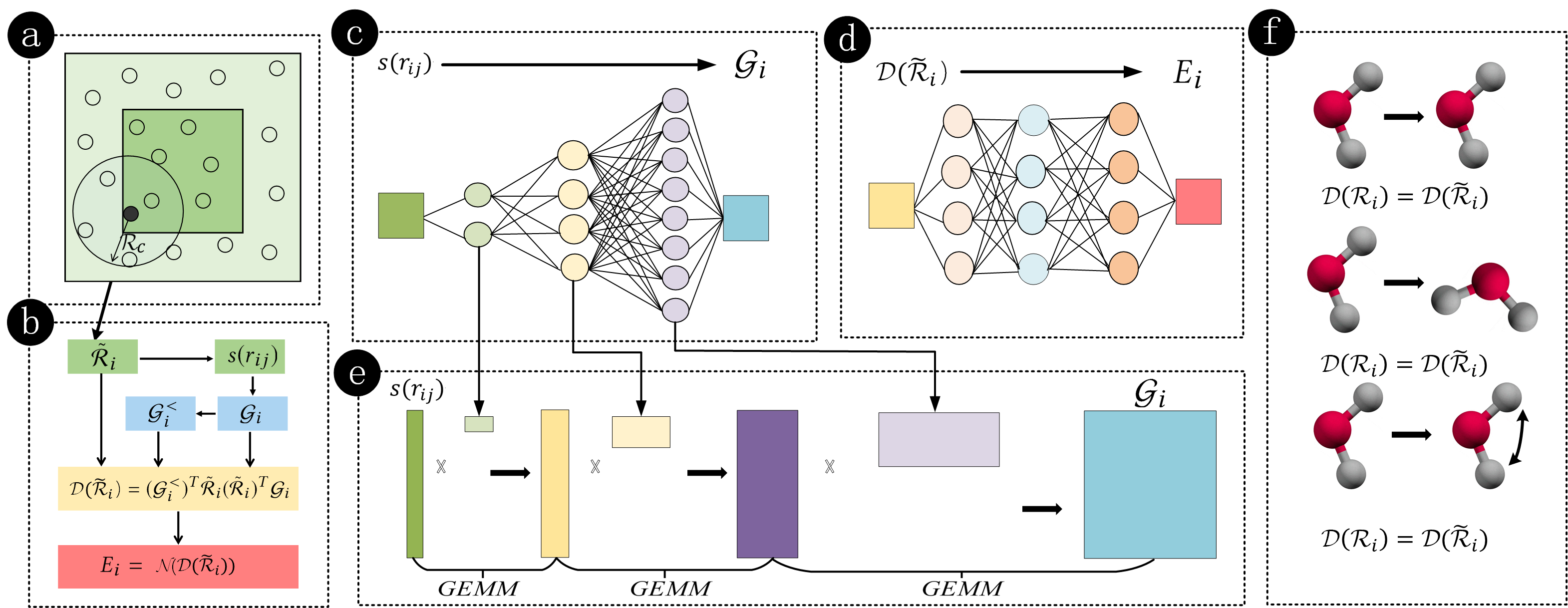
Figure 1. A schematic illustration of the DP model. (a). One sub-region on a single MPI task (Green: local region, light cyan: ghost region). (b). The mapping from local environment $\tilde{\mathcal{R}_{i}}$ to the energy $E_{i}$ for a single atom. (c). Embedding net with three hidden layers. (d). Fitting net with three hidden layers. (e). Execution of the embedding net of the previous DP model via matrix-matrix multiplications, the first layer expands vector $s(r_{ij})$ by a factor of $d_{1}$, the next two layers expand the input matrix by a factor of two. (f). Physical symmetry preserving descriptors.

A detailed mathematical view of the model is the following: The input of the DP model is the environment matrix of each atom $i$, which is denoted as $\tilde{\mathcal{R}_{i}}\in\mathbb{R}^{N_{m}\times 4}$, where $N_{m}$ is the maximum of all neighbor list. $\tilde{\mathcal{R}_{i}}$ is constructed from the local environment, i.e. all relative postitions of neighboring atoms $\bm{r_{ij}}=\bm{r_{j}}-\bm{r_{i}}=\{x_{ij},y_{ij},z_{ij}\}$, with the following equations:

(1) $$\tilde{\mathcal{R}_{i}}=s(r_{ij})\times(1,x_{ij}/{|\bm{r_{ij}}|},y_{ij}/{|\bm{r_{ij}}|},z_{ij}/{|\bm{r_{ij}}|}),$$

where $s(r_{ij})=\omega(|\bm{r_{ij}}|)/{|\bm{r_{ij}}|}$ and $\omega(|\bm{r_{ij}}|)$ is a gating function that decays smoothly from $1$ to $0$ when $|\bm{r_{ij}}|\leq R_{c}$. The DP model is unique in automatically generated descriptors $\mathcal{D}({\tilde{\mathcal{R}}_{i}})$, which preserved physical symmetries such as translational, rotational, and permutational invariance:

(2) $$\mathcal{D}(\tilde{\mathcal{R}}_{i})=(\mathcal{G}_{i}^{<})^{T}\tilde{\mathcal{R}_{i}}(\tilde{\mathcal{R}_{i}})^{T}\mathcal{G}_{i},$$

where $\mathcal{G}_{i}\in\mathbb{R}^{N_{m}\times M}$ is the embedding matrix as illustrated in Fig. 1(b). The matrix $\mathcal{G}_{i}$ obtained by forwarding vector $s(r_{ij})$ through the $m$-layer fully connected embedding net (see Fig. 1 (c)):

(3) $$\mathcal{G}_{i}=\mathcal{L}_{m}^{e}\circ\dots\circ\mathcal{L}_{1}^{e}\circ\mathcal{L}_{0}^{e}(s(r_{ij})).$$

The first layer is a standard fully-connected layer with activation function $\tanh$:

(4) $$\mathcal{L}_{0}^{e}(x)=\tanh(x\cdot W_{0}^{e}+b_{0}^{e}),\quad W_{0}^{e}\in\mathbb{R}^{d_{1}},b_{0}^{e}\in\mathbb{R}^{d_{1}}.$$

The input size is expanded by $d_{1}$ times after the first layer. The rest layers are fully-connected layers with shortcut connection and $\tanh$ activation function:

(5) $$\mathcal{L}_{k}^{e}(x)=(x,x)+\tanh(x\cdot W_{k}^{e}+b_{k}^{e}).$$

The output size of each layer is doubled and final output size is $M$ (see Fig. 1 (e), note $M=4d_{1}$). The matrix $\mathcal{G}_{i}^{<}\in\mathbb{R}^{N_{m}\times M^{<}}$ with $M^{<}<M$ is a sub-matrix of $\mathcal{G}_{i}$ formed by taking the first $M^{<}$ columns of $\mathcal{G}_{i}$.

The symmetry-preserving descriptor $\mathcal{D}$ is mapped to ato-mic energy $E_{i}$ via a fitting network $\mathcal{N}$: $E_{i}=\mathcal{N}(\mathcal{D}(\tilde{{\mathcal{R}}}_{i}))$ (see Fig. 1 (d)). The fitting network $\mathcal{N}$ is a standard fully-connected network with hidden layers being of the same size. A shortcut connection is established between the input and output of each hidden layer of the fitting network. The force on atom $i$ is derived from the negative gradient of the total energy: $F_{i}=-\nabla_{r_{i}}E=-\sum_{j}\nabla_{r_{i}}E_{j}$.

2.2. Computationally intensive parts and memory footprint

Both the training and inference of the DP model are implemented  in  an  open-source  package  DeePMD-kit(Zhang et al., 2018a).  DeePMD-kit is further interfaced with the LAMMPS package (Plimpton, 1995) to perform large-scale MD simulations. The model training generally takes a few hours to one week on a single GPU, depending on the complexity of the physical system (Zhang et al., 2018b). The model inference, on the other hand, can take hours, even days on supercomputers for simulating a large system with long time scales. Thus, in this work, we focus on the computationally intensive part, i.e., the inference of the DP model.

TensorFlow is selected as the framework for building the DP model. All procedures listed in Fig. 1 are implemented either with standard TensorFlow operators or with customized TensorFlow operators. For example, both embedding net and fitting net are constructed with standard TensorFlow operators, and the environment matrix $\tilde{\mathcal{R}_{i}}$ is built via hand-crafted TensorFlow operators.

The most computationally intensive part of the DP model lies in attaining the embedding matrix from $s(r_{ij})$ via the embedding net, as illustrated in Fig. 1 (e). Profiling of the previous DeePMD-kit shows that more than $90$ percent of the total time are spent on execution of the embedding net. The input vector $s(r_{ij})$, which is a smooth function of $\frac{1}{|r_{ij}|}$(see Sec. 2.1), is expanded from size $N_{m}$ to $N_{m}\times 4d_{1}$ by matrix-matrix multiplication operations, where $N_{m}$ is the max length of all atomic neighbor lists and $d_{1}$ is the width of the first fully connected layer. Theoretically, the total FLOPs of the embedding net is $N_{a}\times(N_{m}\times d_{1}+10\times N_{m}\times d_{1}^{2})$, where $N_{a}$ stands for the number of atoms residing on single MPI task. For example, $N_{a}$ can be up to $4,600$ and $N_{m}$ is $512$ for the copper system in the previous work(Jia et al., 2020), and the corresponding width of the three fully connected layers in the embedding net are 32, 64, and 128, respectively. The computational cost of the embedding net approximately accounts for $95\%$ of the total FLOPs. It is noted that the embedding matrix $\mathcal{G}_{i}$ (dimension: $N_{a}$$\times$$N_{m}$$\times$$128$) is the most memory-demanding variable in the DeePMD-kit. For example, $\mathcal{G}_{i}$ can take $2.4$GB GPU global memory for a system of $4,600$ copper atoms mentioned above. Since several copies of $\mathcal{G}_{i}$ are required during the model inference, such as in forward and backward propagation, trading time with space, etc., the $\mathcal{G}_{i}$ related memory consumption accounts for more than $95\%$ of the total.

3. INNOVATION

3.1. Summary of contributions

The main contribution of this paper is a performance portable DeePMD-kit code, which further extends the system size and time scale of molecular dynamics with ab initio accuracy on modern HPC platforms. The optimization strategy and implementation details are summarized on both Fugaku and Summit, providing insights to the optimization of other HPC applications.

3.2. Algorithmic innovation

As discussed in Sec. 2.2, the propagation of the embedding net accounts for $95\%$ of the FLOPs in the baseline implementation, and takes more than $90\%$ of the total time. The reason, as shown in Fig. 1 (e), lies in the computational expense of matrix-matrix multiplications, which rapidly increases through each layer of the embedding net. The embedding matrix $\mathcal{G}_{i}$ is expanded from one vector $s(r_{ij})\in\mathbb{R}^{N_{m}}$ by $M$ times in this process, and reaches $N_{m}\times M$ after the propagation of the embedding net. Essentially, embedding net can be viewed as a mapping function $g:\mathbb{R}\to\mathbb{R}^{M}$, from each component of the vector $s({r_{ij}})$ to one row of the embedding matrix $\mathcal{G}_{i}$. By employing Equations 4 and 5 in Sec. 2.1 as activation functions, the embedding net is a high-dimensional and extraordinarily complex continuous function(Lu et al., 2020).

Weierstrass Approximation Theorem 1.

Suppose $g$ is a continuous real-valued function defined on the real interval $[a,b]$. For every $\varepsilon>0$, there exists a polynomial $f$ such that for all $x$ in $[a,b]$, we have $|f(x)-g(x)|<\varepsilon$, or equivalently, the supremum norm $\|f(x)-g(x)\|<\varepsilon$.

Based on the Theorem 1, polynomials can be introduced to approximate the embedding network. The domain of the input is equally divided into $n$ intervals with nodes denoted by $x_{0}<x_{1}<\dots<x_{n}$. In the $\theta$-th interval $(x_{\theta-1},x_{\theta}],\theta=1,2,\dots,n$, we approximate the embedding net with $M$ fifth-order polynomials

$$f_{\theta}^{\eta}(x)=a_{\theta 0}^{\eta}+a_{\theta 1}^{\eta}x+a_{\theta 2}^{\eta}x^{2}+a_{\theta 3}^{\eta}x^{3}+a_{\theta 4}^{\eta}x^{4}+a_{\theta 5}^{\eta}x^{5}.$$

In order to determine the coefficients $a_{\theta\xi}^{\eta}$, $\xi=0,1,2,3,4,5$, $\eta=1,2,\dots,M$, we acquire the values, first and second order derivatives of $f_{\theta}$ and $g$ matched at the nodes $x_{\theta-1}$ and $x_{\theta}$. The obtained coefficients $a_{\theta\xi}^{\eta}$ are gathered and stored as a table, so that the evaluation of the original embedding net now can be approximated by the polynomials. This procedure is also referred as tabulation in this work. The accuracy of the tabulation relies on the size of the interval $(x_{\theta-1},x_{\theta}]$. With a decreasing interval size, the error introduced by the approximation would vanish.

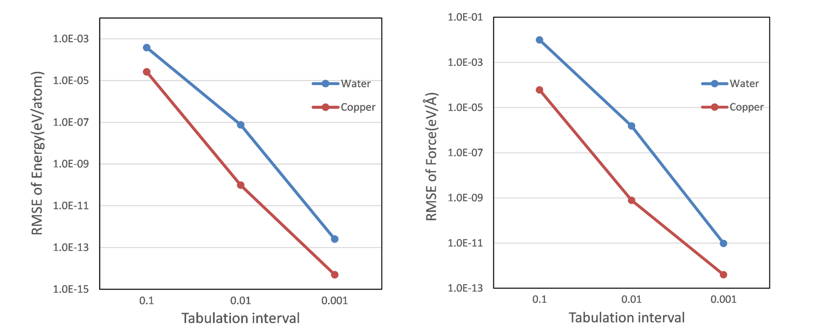
Figure 2. Accuracy of the tabulated model compared to the baseline DP model. Root mean squared error (RMSE) of per-atom energy and per-component force are shown, with respect to 3 interval sizes (0.1, 0.01, and 0.001). 100 data are tested for each system.

Two physical systems, water and copper, are tested to show the accuracy of the tabulated DP model against the baseline in Fig. 2. The accuracy is measured by the root mean square error (RMSE) in predicted per-atom energy ($RMSE_{E}$) and per-component force ($RMSE_{F}$), i.e.,

$$RMSE_{E}=\frac{1}{N}{\sqrt{\frac{1}{m}\sum\nolimits_{i=1}^{m}{(E_{i}^{tab}-E_{i}^{orig})^{2}}},}$$

and

$$RMSE_{F}={\sqrt{\frac{1}{3mN}\sum\nolimits_{i=1}^{m}\sum\nolimits_{j=1}^{N}\sum\nolimits_{k=1}^{3}(F_{i,j,k}^{tab}-F_{i,j,k}^{orig})^{2}}},$$

where $m$ is the number of data to be tested (the number of atomic configurations), $N$ is the number of atoms in each configuration and $k$ represents three directions of Cartesian coordinates. Quantities with superscripts $tab$ and $orig$ denote the predictions of the tabulated DP model and the original DP model, respectively. As shown in Fig. 2, the RMSE of the per-atom energy drop from $2.0\times 10^{-5}$ eV/atom to $5.0\times 10^{-15}$ eV/atom and the corresponding per-component force drop from $6.0\times 10^{-5}$ eV/$\Angstrom$ to $4.0\times 10^{-13}$ eV/$\Angstrom$ when the interval varies from $0.1$ to $0.001$. Note that the double-precision limit is reached when the interval is set to $0.001$. This means our tabulated model can be equally accurate as the original model. We remark that the size of the tabulated model grows as the interval decreases. For example, the size of the model can be 257 MB for water system when interval equals $0.001$, but only 33 MB when the interval is $0.01$. Thus in practice, an optimal interval is balanced between accuracy and model size, and we choose $0.01$ as default in our optimized code.

A theoretical analysis of the FLOPs on embedding matrix for both the original and tabulated model is as follows. We denote the number of atoms by $N_{a}$, the maximal neighbor list size by $N_{m}$ and the size of the first layer of the embedding net by $d_{1}$. For the purpose of simplicity, the FLOPs of activation function are counted. The total number of FLOPs for computing the three-layer embedding net by the original model is $N_{a}\times(N_{m}\times d_{1}+10\times N_{m}\times d_{1}^{2})$, as discussed in Sec. 2.2, while that for the tabulated model is $N_{a}\times 56\times N_{m}\times d_{1}$. Thus, the theoretical speedup in terms of FLOPs is: $\nicefrac{{(1+10\times d_{1})}}{{56}}$. In the previous work(Jia et al., 2020), $d_{1}$ is set to be $32$ for both water and copper systems, thus the tabulated model saves $82$ percent of the embedding matrix FLOPs compared to the original model.

3.3. Optimization strategy

In this section, we will discuss the general strategies used in optimizing DeePMD-kit on modern many-core architectures. The goal is to reduce the memory footprint after the total FLOPs are brought down by 82 percent by the tabulation of embedding net as discussed in Sec. 3.2.

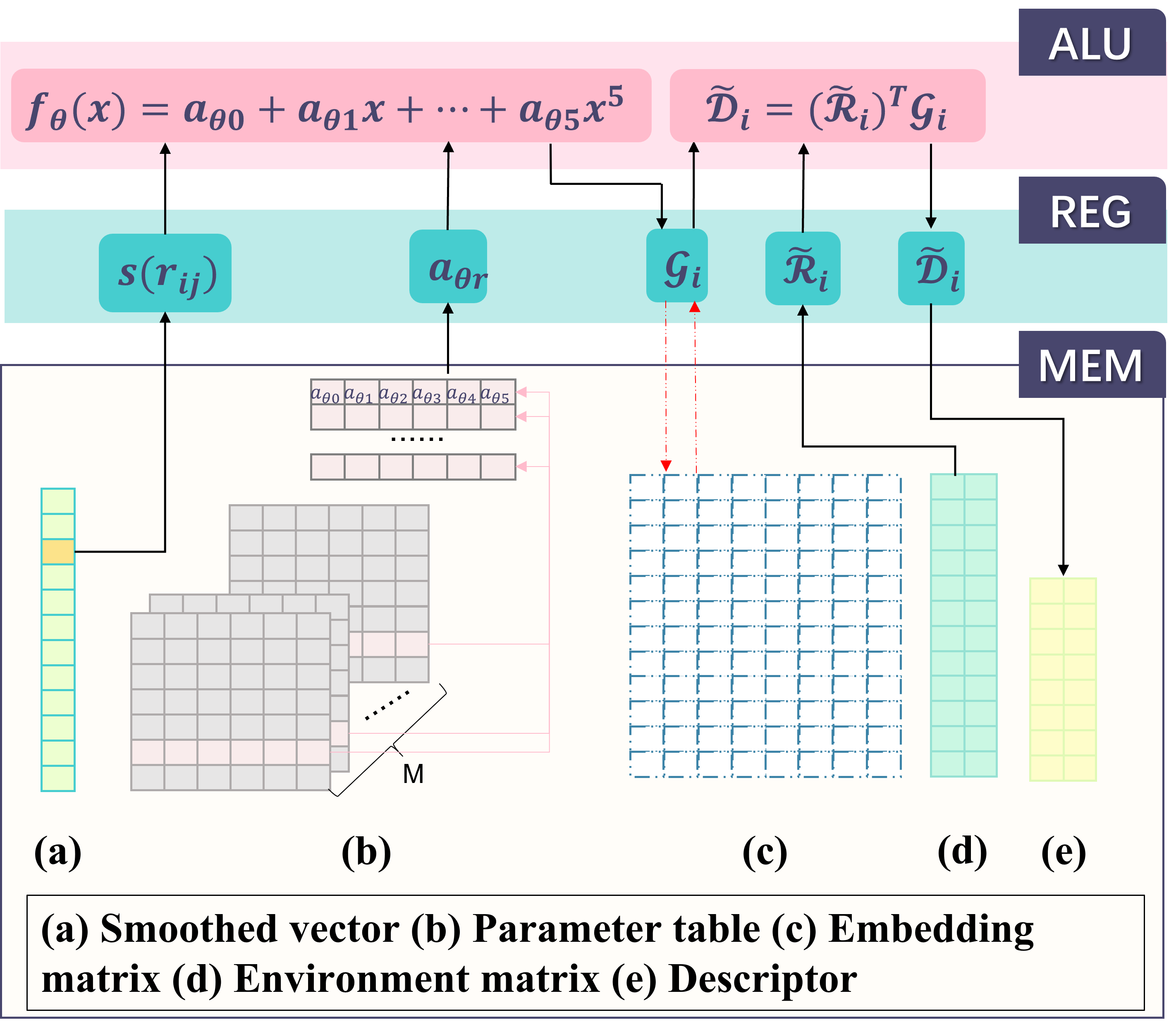
Figure 3. An illustration of the data movement when evaluating the descriptor $\mathcal{D}_{i}$ of the optimized (tabulated and kernel fused) DP model. Dashed line: memory allocation/access saved by the kernel fusion.

The first strategy is to reduce the memory footprint by contracting variables and merging calculations. We find that the embedding matrix $\mathcal{G}_{i}$, as discussed in Sec. 2.2, is the most memory-demanding variable and takes more than $95$ percent of the total memory usage in the baseline implementation. After the tabulation of the embedding net (See Sec. 3.2), $\mathcal{G}_{i}$ is no longer built through the three-layer embedding net (Fig. 1 (e)), rather, it is approximated by fifth-order interpolations. The data movement of evaluating the descriptor $\mathcal{D}_{i}$ on typical modern many-core architecture is illustrated in Fig. 3. For simplicity, we only demonstrate the data movement among the basic components such as arithmetic logic unit (ALU), register (REG), and high-bandwidth memory (MEM). CACHE and shared memory are not discussed. The tabulation of embedding net ($f_{\theta}(x)=a_{\theta 0}+a_{\theta 1}x...a_{\theta 5}x^{5}$) loads the vector $s(r_{ij})$ and the parameter table, and stores the embedding matrix $\mathcal{G}_{i}$. Then $\tilde{\mathcal{R}_{i}}^{T}\mathcal{G}_{i}$ is carried out by calling the matrix-matrix multiplication (GEMM) subroutine. We optimize the allocation and access of $\mathcal{G}_{i}$ by contracting the tabulation and matrix-matrix multiplication, and the resulting equation is $\tilde{\mathcal{R}_{i}}^{T}f_{\theta}(s(r_{ij}))$. Although the contracted equation saves the load and store of the embedding matrix $\mathcal{G}_{i}$, implementation detail still vary depending on the architecture, as will be discussed in Sec. 3.4 and Sec. 3.5.

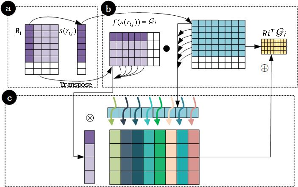
Figure 4. Removing the redundant zeros from the DP model. (a) Redundant zeros in the environment matrix $\mathcal{R}_{i}$, $s(r_{ij})$. (b) Evaluation of ${\mathcal{\tilde{R}}_{i}}^{T}\mathcal{G}_{i}$. Note that redundant-zero ratio of the embedding matrix $\mathcal{G}_{i}$ are related to the $s(r_{ij})$. (c) Bypassing redundant zeros in the execution of outer product in one thread block.

Removing redundancy is the second strategy used in our optimization. Related work demonstrated that up to 52 percent of performance boost can be gained in removing calculations related to redundant zeros (You et al., 2020). In the previous DP model, the data redundancy stems from the padding of the number of rows of the environment matrix $\mathcal{\tilde{R}}_{i}$ to $N_{m}$, where $N_{m}$ is the maximally possible length of atomic neighboring list as discussed in Sec. 2. Then the padded matrix can take advantage of the high-performance matrix-matrix multiplication by calling the GEMM subroutine. However, since the tabulation of the embedding matrix and the consecutive GEMM operations are merged as discussed above, the redundancy related operations can also be bypassed. Note that data redundancy exists not only in $\mathcal{R}_{i}$, but also in $s(r_{ij})$ and the corresponding embedding matrix $\mathcal{G}_{i}$ (Fig. 4 (a)). The size of $N_{m}$ can be as large as several hundred, depending on the cutoff radius $R_{c}$. For example, $N_{m}$ is set to be $128$ and $512$ for the water and copper systems, respectively (Jia et al., 2020). The copper model is trained for both ambient and high-pressure conditions, while the water model is trained only for ambient conditions. The $N_{m}$ reserved for the copper model is larger because the neighbor lists are longer in the high-pressure conditions (higher density and thus more neighbors in the cutoff radius). When the models are used under ambient conditions, the copper model has a higher degree of redundancy, and the redundancy can not be avoided nor reduced due to the data layout and matrix operations in the baseline implementation.

The third optimization strategy is to improve the parallel efficiency by increasing the computational granularity of each individual MPI process. We notice that given a fixed physical problem, the ratio between computation over communication decreases as we use more MPI tasks. This is mainly because the communication volume of the ghost region increases when using more MPI tasks. For example, in a one-dimensional problem, suppose the size of the ghost region of an individual MPI is $V$ and the total number of MPI process is $n$, then the communication volume of the ghost region is $n\times V$. This means theoretically, it is optimal to launch only one MPI per node and distribute the workload into finer granularity by using OpenMP, CUDA, etc… In practice, MPI+X is the most frequently used parallelization schemes, and X can be OpenMP, CUDA, HIP, etc.

3.4. Implementation I: GPU

In the following subsections, we will focus on optimizing the DeePMD-kit on the GPU heterogeneous architecture based on the strategies outlined in Sec. 3.3 .

3.4.1. Kernel fusion

We optimize the GPU memory footprint by merging the tabulation of the embedding net and consecutive matrix-matrix multiplication into a single CUDA customized kernel. In the optimized DeePMD-kit, each row of $\mathcal{G}_{i}$ is evaluated in one thread block and stored in the register (without storing back to global memory), then one column of the environment matrix $\tilde{\mathcal{R}_{i}}^{T}$ is loaded into the registers to perform an outer product. An illustration of the outer product is shown in Fig. 4. The result from all thread blocks is added up to from $\tilde{\mathcal{R}_{i}}^{T}\mathcal{G}_{i}$. Note that the dimension of the outer product matrix is $4\times M$, and can be accommodated in the shared memory on V100 GPUs for an efficient summation. We remark that $\mathcal{G}_{i}$ is neither allocated nor moved between global memory and registers in the optimized code, and both the memory footprint and computational time are significantly reduced after the kernel fusion, as will be discussed in Sec. 6.

3.4.2. Redundancy removal

The fused CUDA kernel introduced in Sec. 3.4.1 makes it possible to bypass the redundant zeros in the DP model. As shown in Fig. 4, one column of $\tilde{\mathcal{R}_{i}}^{T}$, together with one row of $\mathcal{G}_{i}$, are held by one thread block to perform an outer product. The dimension of the resulting matrix $\tilde{{\mathcal{D}_{i}}}=\tilde{\mathcal{R}_{i}}^{T}\mathcal{G}_{i}$ is $4\times M$, where $M$ is typically $128$. Note that if element $j$ in $s(r_{ij})$ is padded, the corresponding column $j$ of $\tilde{\mathcal{R}_{i}}^{T}$ and row $j$ of $\mathcal{G}_{i}$ are also padded with constant numbers. Thus, the corresponding final results can be directly derived without any floating-point operations.

3.4.3. Other optimizations

The customized TensorFlow operators are also accelerated. For example, ProdEnvMatA, which evaluates the environment matrix from the neighbor list of atom $i$, is further optimized on GPU by carefully using shared memory and removing redundancy. Testing results show that the optimized version can be 3 times faster compared to the original one. A random global memory writing policy is applied to ProdForceSeA and ProdVironSeA, which are operators for computing the forces and virial tensors, and improves the performance of atomic addition.

3.5. Implementation II: ARM CPU

Starting from a flat MPI version of the DeePMD-kit (Jia et al., 2020), we apply the optimization strategies listed in Sec. 3.3 on the Fugaku supercomputer in the following subsections.

3.5.1. Tabulation of embedding net

In our previous implementation, the fifth-order tabulated model introduced in Sec.  3.2 are stored as an array of structures (AoS). The 6 coefficients of the polynomials are stored continuously as a row. However, AoS can not fully exploit the 1024 GB/s bandwidth provided by the A64FX CPU due to the discontinuous memory access. We optimize the data layout of the tabulated model by transposing every 16 structures so that the 512-bit scalable vector extension (SVE) instructions are invoked in accessing the table. Note that 16 is chosen because the loop is unrolled two times to take advantage of the two floating-point operation pipeline on A64FX($16\times 64=1024$ bits). We remark that the data layout of the tabulated model is not transposed during the MD simulation, but during the tabulation as part of the post-processing.

3.5.2. Kernel fusion and redundancy removal

The tabulation of the embedding net and consecutive matrix-matrix multiplication are merged into a single function, and then the FLOPs with respect to redundant elements are avoided on A64FX. The outer product of the environment matrix $\tilde{\mathcal{R}_{i}}^{T}$ and the embedding matrix $\mathcal{G}_{i}$ is implemented on the ARM CPU to enhance the 64 KB L1 CACHE hit rate. We remark that the implementation of the kernel fusion and redundancy removal follows the same pattern on both A64FX and V100 GPU.

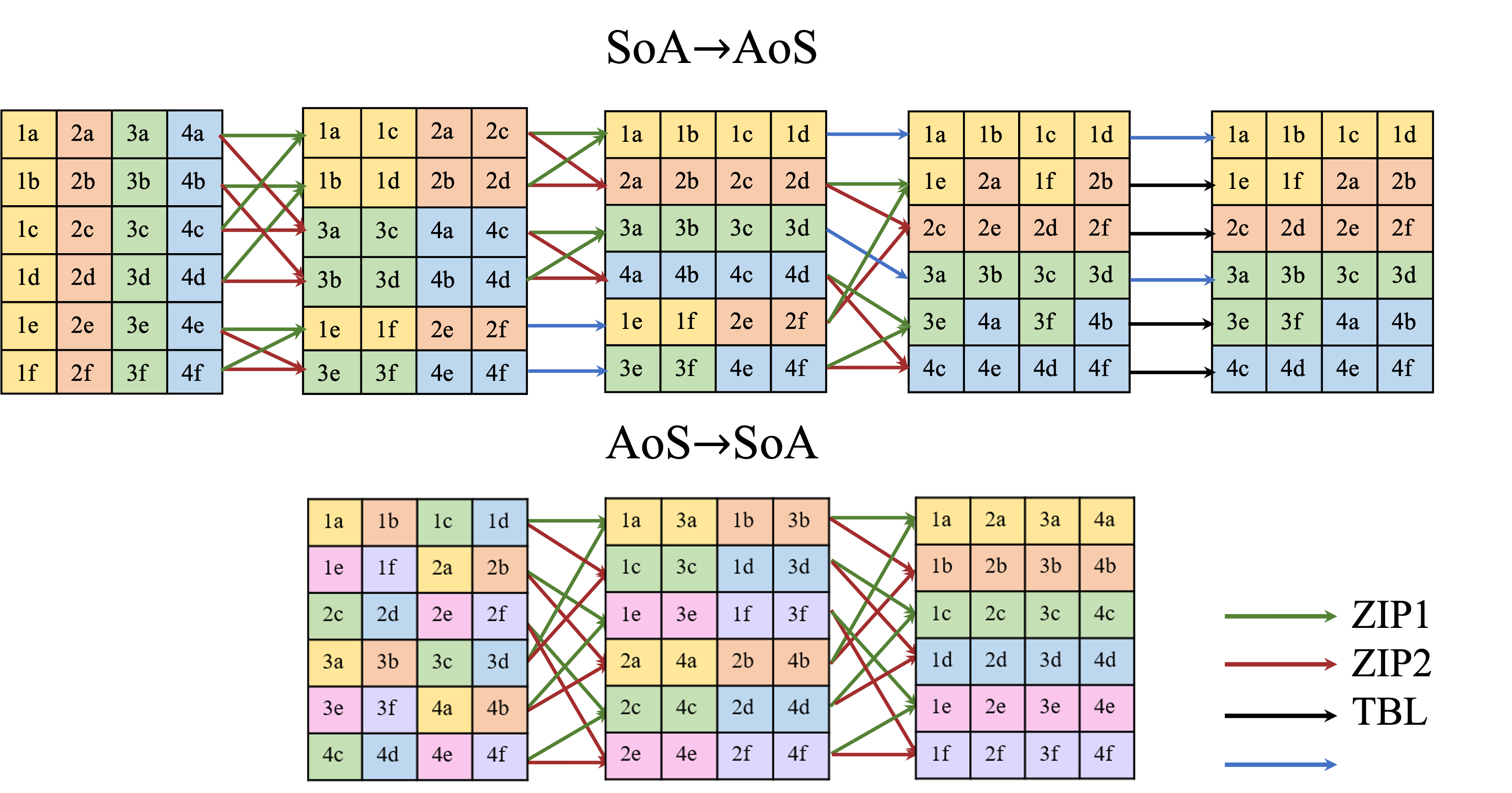
Figure 5. An illustration of converting between AoS and SoA by utilizing SVE instructions. Conversion of 6x4 arrays is plotted for simplicity. Each row is a vector register or is stored continuously in memory.

3.5.3. Other optimizations

We further optimize the customized TensorFlow operators by exploiting vectorization. One key data structure is descrpt_a_deriv which is used in multiple customized TensorFlow operators such as ProdEnvMatA, ProdViralSeA and ProdForceSeA. The variable descrpt_a_deriv is stored as an AoS, and is required to be converted between SoA and AoS for vectorization purposes. For AoS of the size of 2$\times$8, 3$\times$8, and 4$\times$8, the conversion can be performed with single ld2, ld3, or ld4 SVE instructions, respectively. However, in the DeePMD-kit, the size of descrpt_a_deriv is 12$\times$8 and can not be trivially converted with single SVE instruction. We implement a fast converting subroutine to switch between SoA and AoS by utilizing 512-bit SVE instructions, as illustrated in Fig. 5. Then the corresponding customized TensorFlow operators are unrolled and vectorized to exploit the computing power of A64FX.

The $\tanh$ function is selected as the activation function for both embedding and fitting net due to accuracy considerations (Zhang et al., 2018a), and it is optimized with a second-order polynomial approximation. Only the positive part of the function is tabulated because it is an odd function ($\tanh(-x)=-\tanh(x)$). The upper bound of $x$ is chosen to be $8$, and for any $x$ greater than $8$, $\tanh(x)$ is set to $1.0$. Our tabulation of the $\tanh$ function can be 60 times faster compared with the original one on A64FX, and the corresponding error is about $1.0\times 10^{-7}$. It is noted that our tabulation of the $\tanh$ does not affect the overall accuracy of the code.

3.5.4. MPI+OpenMP

Previously, the DeePMD-kit is parallelized on Fugaku in a flat MPI scheme to exploit the performance of many-core architecture, as shown in Fig. 6(a). However, due to the limited size of high bandwidth memory on A64FX (32GB), each MPI task can only allocate a maximum of 0.67GB memory (32GB/48=0.67GB). Thus the size of the sub-region resides on a single MPI task is highly restricted by the memory available. Furthermore, the TensorFlow graph, along with MPI buffers, are allocated and kept 48 copies on a single Fugaku node and deteriorate the situation. A hybrid parallelization scheme using MPI+OpenMP can effectively reduce the number of MPI used, increasing parallel granularity and reducing inter-MPI communication, as discussed in Sec. 3.3. We find that intra-operators MPI+OpenMP parallelization (See Fig. 6(b)) is not efficient due to frequently forking and joining between different operators. And some customized TensorFlow operators, such as ProdVirialSeA, ProdForceSeA, having writing conflicts and can not be easily parallelized with OpenMP.

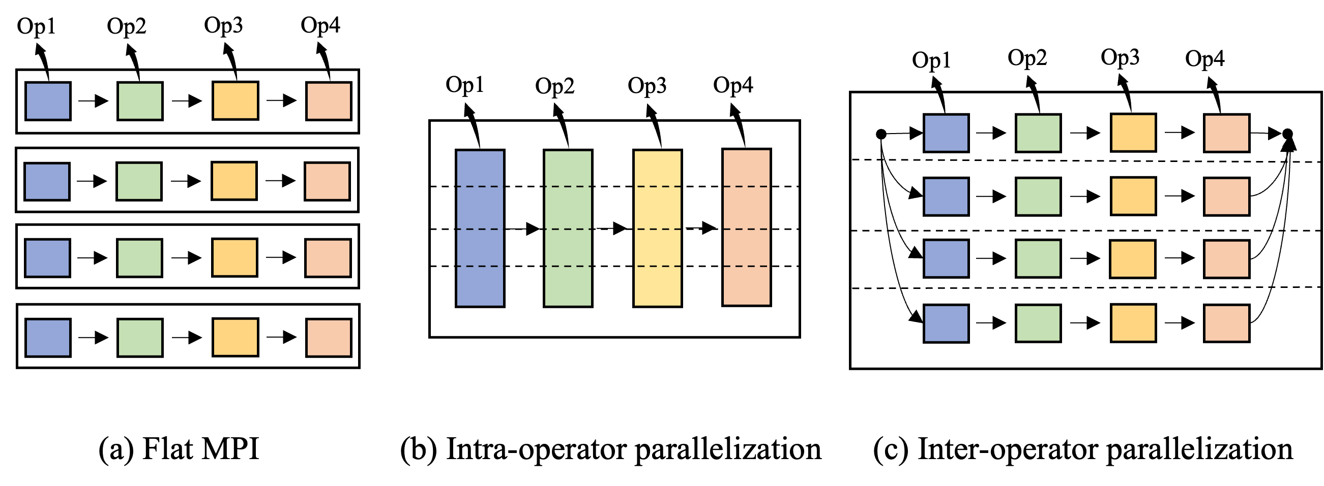
Figure 6. Hybrid paralllelization scheme including (a) Flat MPI parallelization, (b) each TensorFlow operator is parallelized among multiple threads in single MPI, and (c) each OpenMP thread holds a fraction of the sub-region and executed in parallel.

Then we implement an inter-operator parallelization scheme, as shown in Fig. 6(c). In this scheme, each OpenMP thread mimics the behavior of an MPI task by holding a fraction of the sub-region. Note that the sub-region is carefully divided to avoid load-balance problems, and thread forking and joining only occur once per MD step. In each MPI task, only one copy of the TensorFlow graph is kept and shared among OpenMP threads, and the inter-MPI communication is significantly reduced due to the increase of granularity. The optimized code can accommodate systems 1.5 time bigger compared to the flat MPI implementation. We remark that the performance of the hybrid parallelization scheme is highly related to the memory affinity of the non-uniform memory access (NUMA) node.

4. The physical systems

The performance of the optimized DeePMD-kit is measured on two typical systems: water and copper, which have been extensively trained and studied in Refs. (Zhang et al., 2018a, b), and (Zhang et al., 2020), respectively. The cutoff radius of water and copper systems are chosen to be 6 and 8 Å, and the corresponding maximal number of neighbors are 138 and 500, respectively. In the previous DP model, the sizes of the embedding net and fitting net are set to be $32\times 64\times 128$ and $240\times 240\times 240$, respectively. In the optimized DeePMD-kit code, these models are compressed and tested on both Summit and Fugaku supercomputers.

The strong scaling of the optimized DeePMD-kit is tested using the water system composed of $41,472,000$ and $8,294,400$ atoms on 4,560 computing nodes of Summit and Fugaku, respectively, and the weak scaling is performed using a copper system with 122,779 and 6,804 atoms per MPI task. We remark that our tests do not reach the entire Fugaku supercomputer due to the computing resource accessible to us. The configuration of the water system is made by replicating a well equilibrated liquid water system of 192 atoms, and that of the copper system are generated as perfect face-centered-cubic (FCC) lattice with the lattice constant of 3.634 Å. A total of 99 MD steps evaluated by the Velocity-Verlet algorithm is performed (the energy and forces are evaluated 100 times), and time steps for water and copper systems are chosen to be 0.5 and 1.0 fs, respectively. Temperature is set to 330 K by utilizing random numbers as the initial velocities of atoms. The neighbor list with a 2 Å buffer region is updated every 50 MD steps. The thermodynamic data including the kinetic energy, potential energy, temperature, pressure are collected and recorded in every 50 MD steps.

5. Machine configuration

All numerical tests are performed on two supercomputers: Fugaku and Summit. The Fugaku supercomputer has 157,986 computing nodes and currently ranks No.1 in the top 500 list (Top 500 list, 8 01) with a theoretical peak performance of 537 PFLOPS. Each computing node is equipped with one A64FX, which has 4 internal groups named core memory groups (CMGs). Each CMG consists of 13 processor cores (one for OS activities), an L2 cache, and a memory controller. Each CMG has 8GB second-generation high-bandwidth memory (HBM2), so one A64FX has 32 GB HBM2 in total and the bandwidth is 1024GB/s. The A64FX supports the Scalable Vector Extension (SVE) and the vector length of SVE can be 128, 256, and 512 bits. Theoretical peak performance of A64FX is 3.07/3.38 TFLOPS double-precision operation at 2.0 GHz and 2.2 GHz (auto boost), respectively. The tests on Fugaku are performed with an MPI+OpenMP hybrid parallelization scheme, all threads within an MPI task are bound to an individual NUMA node to take advantage of the CPU-memory affinity.

All GPU-related tests are performed on the Summit supercomputer, which ranks No. 2 in the top 500 list (Top 500 list, 8 01) with a theoretical peak performance of 200 PFLOPS. Summit has 4,560 computing nodes, and each node has 2 identical groups consisting of one IBM POWER 9 socket and 3 NVIDIA V100 GPUs. The two groups of hardware are interconnected via X-Bus with a bandwidth of 64 GB/s. Each IBM POWER 9 socket has 22 CPU cores and is equipped with 256 GB main memory with a bandwidth of 135 GB/s. Each V100 GPU has 16 GB of HBM with a bandwidth of 900 GB/s, and its double-precision theoretical peak performance is 7 TFLOPS. The GPUs within a single group are connected through NVLink with a bandwidth of 50 GB/s. A non-blocking fat-tree topology using dual-rail Mellanox EDR InfiniBand with a bandwidth of 25 GB/s is formed among computing nodes, with one network adapter connected to one group of hardware. We use 6 MPI tasks per computing node in all tests on Summit by binding 3 MPI tasks to each group of hardware (each MPI binds to an individual GPU) to fully exploit the CPU-GPU affinity and network adapter.

6. PERFORMANCE RESULTS

In this section, we test the performance of the DeePMD-kit first on a single GPU and A64FX, and then the scaling behavior on Summit and Fugaku. Note that in all comparisons, the baseline code is the current state-of-the-art (Jia et al., 2020) version of DeePMD-kit.

Figure 7. Step-by-step performance improvement on a single V100 GPU machine using algorithmic and system innovations. Baseline is the results from Ref. (Jia et al., 2020).

6.1. Single V100 GPU

The performance results on $12,880$-atom water and $6,912$-atom copper systems are tested to measure the performance improvement of critical algorithmic and system innovations on a single V100 GPU. The speedup of the time-to-solution for 99 steps of MD based on a step-by-step optimization is shown in Fig. 7.

6.1.1. Tabulation of embedding net

Compared to the baseline, we find that the optimized DeePMD-kit can be $2.3$ and $3.7$ times faster for water and copper system after introducing the tabulation of embedding net. Note that $82$ percent of FLOPS (see Sec. 3.2) are saved by the tabulation, implying a 5.6 times speedup. The actual speedup is less than ideal because DeePMD-kit is memory-bound rather than compute-bound (Jia et al., 2020), the speedup factor is determined by the memory-access reduction in the inference.

6.1.2. Kernel fusion

As detailed in Sec. 3.4.1, both memory footprint and computational time are reduced by merging the tabulation and consecutive matrix-matrix multiplication into a single customized CUDA kernel. Testing results show that the maximum number of atoms accommodated on a single V100 GPU increase by a factor of 6 and 26 for water and copper systems, respectively. The total speedup is $3.1$ and $5.9$ compared to the baseline for water and copper, respectively.

6.1.3. Redundancy removal

As discussed in Sec. 3.4.2, the evaluation of redundant elements is skipped to reduce the floating-point operations. Compared with the baseline, the speedup factor increase to $3.4$ and $8.4$ for water and copper systems, respectively. Profiling results show that our optimized kernel achieves $94\%$ of the 900 GB/s bandwidth provided by the V100 GPU. We remark that copper gains a higher speedup in this step due to a higher degree of redundancy, as discussed in Sec. 3.4.2.

6.1.4. Other optimizations

The customized TensorFlow operators in DeePMD-kit are also optimized, and the corresponding speedup compared to the baseline is shown in Fig. 7. Overall, the time-to-solution of the optimized DeePMD-kit is 3.7 and 9.7 times faster, and system size increase by a factor of 6 and 26 on a single V100 GPU for water and copper, respectively.

6.2. Single A64FX

Two systems, $18,432$-atom water and $2,592$-atom copper, are tested to measure the performance of the optimized DeePMD-kit on a single Fugaku node (A64FX). Note that the baseline is a flat MPI version of DeePMD-kit on A64FX. We remark that the GPU baseline is highly optimized  (Jia et al., 2020), but the A64FX baseline is not optimal and requires further optimization. A step-by-step optimization is detailed at Sec. 3.5, and the corresponding speedup is shown in Fig. 8.

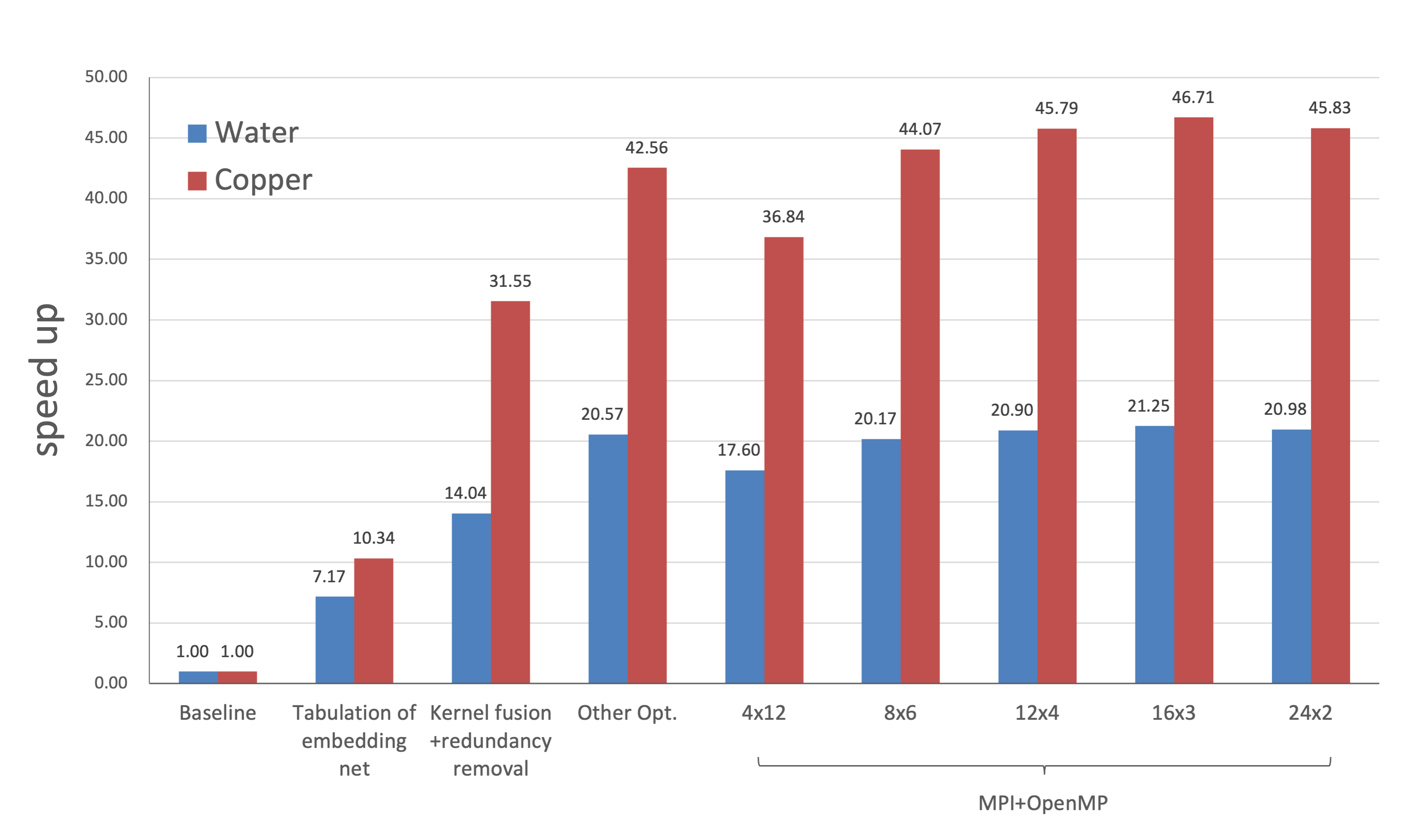
Figure 8. Step-by-step performance improvement on a single A64FX node for the $18,432$-atom water and $2,592$-atom copper systems.

6.2.1. Tabulation of embedding net

The data layout of the tabulated polynomial coefficients is rearranged to take advantage of the 512-bit SVE instructions. As shown in Fig. 8, after rearranging the data layout of the tabulated polynomial coefficients discussed in Sec. 3.5.1, the optimized model can be $7.2$ and $10.3$ times faster compared to the baseline for water and copper, respectively.

6.2.2. Kernel fusion and redundancy removal

We find that the kernel fusion and redundancy removal not only brings significant performance improvement on GPU but also work efficiently on CPU architecture. As shown in Fig. 8, the optimized model can be $14$ and $31.5$ times faster compared to the baseline for water and copper, respectively.

6.2.3. Other Optimizations

The customized TensorFlow operators, such as ProdEnvMatA op, ProdVirialSeA op and ProdForceSeA, are vectorized in the optimized DeePMD-kit, as detailed in Sec. 3.5.3. We achieve an average speedup factor of $1.2$, $8.3$ and $7$ for ProdEnvMatA op, ProdVirialSeA op and ProdForceSeA, respectively. The corresponding proportion of the customized operators decreases from $15\%$ and $25\%$ to $10\%$ and $17\%$ for water and copper, respectively.

Tanh is the activation function used in the DP model, and it takes $32\%$ and $20\%$ of total computational time for water and copper, respectively, on A64FX. In the optimized DeePMD-kit, Tanh is accelerated by tabulation as detailed in Sec. 3.5.3. We achieve a speedup of $66.4$ and $44.5$ times for water and copper systems without any loss of accuracy. As shown in Fig. 8, the overall speedup factor reaches $20.5$ and $42.5$ for water and copper systems, respectively.

6.2.4. MPI+OpenMP

MPI+OpenMP parallelization is introduced into the optimized DeePMD-kit to save memory usage and inter-MPI communication on the many-core architecture, as discussed in Sec. 3.5.4. The extra copies of the TensorFlow graph and system buffers are no longer needed. The system size accommodated on single A64FX node increase from $110,592$ to $165,888$ when using a 16$\times$3 configuration for water. Note that because the TensorFlow graph for the copper system is small (13 MB), the system size of copper using MPI+OpenMP almost remains the same as the flat-MPI version. Testing results show that MPI+OpenMP implementation can also be slightly faster than the flat MPI except when using 4$\times$12 (Each MPI task consists of 12 threads, and resides on an individual CMG), as shown in Fig. 8. Since the 16$\times$3 configuration is the optimal choice both in system size and computational speed, we use 16$\times$3 as the configuration in the scaling tests.

6.3. Comparison between A64FX and V100

Table 2. Comparison between A64FX and V100: the time-to-solution (TtS) (in us/step/atom), the normalized time-to-solution with respect to FLOPS (TtS$\times$Peak), and the normalized TtS with respect to power consumption (TtS$\times$Power) are listed. Numbers in brackets are speedup factors as compared to the V100 results.

		TtS	TtS $\times$ Peak	TtS $\times$ Power
Summit	water	2.58	18.1(1.0)	952.0(1.0)
	copper	2.87	20.1(1.0)	1059.0(1.0)
Fugaku	water	4.47	15.1(1.2)	737.6(1.3)
	copper	5.78	19.5(1.03)	953.7(1.1)

For the water system, we achieve 4.47 us/step/atom with one A64FX and 2.58 us/step/atom with one V100 GPU. The time-to-solution is normalized for a fair comparison, as shown in Table 2. First, we normalize the time-to-solution with respect to peak performance by multiplying time-to-solution with the theoretical peak of V100 and A64FX. We find that the normalized results on A64FX can be $1.2$ and $1.03$ times faster than V100 for water and copper systems, respectively. The average power consumption of a single V100 and A64FX is 369 and 165 watts (Top 500 list, 8 01), respectively. Then the time-to-solution is normalized with respect of power consumption, as shown in Table 2. By setting V100 as the baseline, the speedup factor of A64FX is 1.3 and 1.1 for water and copper, respectively.

6.4. Scaling

The scalability of our optimized DeepMD-kit is evaluated on Summit and Fugaku. Note that a fraction of the Fugaku supercomputer is used due to the computational resource accessible to us. The system size can reach an unprecedented $17$ billion atoms, $134$ times bigger compared to the current state-of-the-art. And the corresponding time-to-solution can be $3.7$ to $9.7$ times faster compared to Ref. (Jia et al., 2020). Note that in all scaling tests, we use an MPI+OpenMP parallelization configuration of $16\times 3$.

6.4.1. Strong Scaling.

Figure 9. Strong scaling of MD simulations (99 steps, atomic forces and the total energy are computed 100 times) for the water system: a total of $8,294,400$ atoms on Fugaku and $41,472,000$ atoms on Summit are used.

Figure 10. Strong scaling of MD simulations (99 MD steps, atomic forces and the total energy are evaluated 100 times) for the copper system: a total of $2,177,280$ atoms on Fugaku and $13,500,000$ atoms on Summit are adopted in these MD simulations.

We measure the scalability of the optimized DeePMD-kit using the parallel efficiency of water ($8,294,400$ atoms for Fugaku, $41,472,000$ atoms for Summit) and copper ($2,177,280$ atoms for Fugaku, $13,500,000$ for Summit) systems. The scaling behavior ranging from $20$ to $4,560$ computing nodes of Summit and Fugaku are nearly the same, as shown in Fig. 9 and Fig. 10. Both water and copper show nearly perfect scaling on up to $570$ and $285$ computing nodes, and can further scale to $4,560$ computing nodes. For the water system, the parallel efficiency is $46.99\%$ on $4,560$ computing nodes on Summit, and that of the Fugaku is $41.20\%$. The corresponding time-to-solution is $6.0$ and $2.1$ nanoseconds per day on Summit and Fugaku, respectively. For the copper system, the parallel efficiency on $4,560$ Summit nodes is $35.96\%$, and the corresponding parallel efficiency is $32.76\%$ for Fugaku. The corresponding time-to-solution can reach $11.2$ and $4.7$ nanoseconds per day.

We notice that the parallel efficiency on Summit is slightly better compared to that on Fugaku due to its higher ratio in computation over communication. Since the computational complexity of DP method is linear ($O(N)$), the ratio of computation over communication can be approximated with the size of the sub-region over the size of the ghost region. Note that we launch 16 MPI tasks on single A64FX node, but only 6 MPI process on one Summit node. When scaling to $4,560$ computing nodes, $72,960$ MPI tasks and $27,360$ MPI tasks are launched on Fugaku and Summit, respectively. In the strong scaling of the copper system, each MPI task on Fugaku holds a sub-region of $113$ atoms, and its ghost region is $1,735$. Meanwhile the corresponding number on Summit is $1,515$ and $7,520$, respectively. The ratio of the computation over communication is $\nicefrac{{1}}{{15}}$ and $\nicefrac{{1}}{{5}}$ on Fugaku and Summit, respectively.

6.4.2. Weak Scaling.

Figure 11. Weak scaling of water and copper systems ranging from $\nicefrac{{1}}{{256}}$ to the entire machine (Summit and Fugaku). Note that the dotted line for Fugaku is a projected result due to the limited computing resources.

The weak scaling of the optimized DeePMD-kit is measured in terms of the system size and FLOPS of 99 MD steps for both water and copper systems (Fig. 11). As shown in Fig. 11, both systems show perfect scaling with respect to the number of nodes used on Fugaku and Summit. On Fugaku, the maximal number of atoms for water and copper can reach $1.56$ and $1.08$ billion atoms, respectively, on $9,936$ nodes, and a projected estimation shows that the DeePMD-kit can reach $24.9$ and $17.3$ billion atoms for water and copper, respectively. We remark that our estimation of the weak scaling is reasonable based on the communication pattern of the DeePMD-kit. For the copper system, the time-to-solution can reach $4.1\times 10^{-11}$ seconds/step/atom, and the corresponding peak performance achieved is $119$ PFLOPS ($22.17\%$ of the theoretical peak). Compared to the current state-of-the-art, the projected system size is 134 times bigger and the corresponding time-to-solution can be $20$ times faster. On Summit, the maximum number of atoms can reach $3.9$ and $3.4$ billion atoms for water and copper, respectively. For the copper system, the time-to-solution can reach $1.1\times 10^{-10}$ seconds/step/atom, and the corresponding peak performance achieved is $43.7$ PFLOPS ($22.8\%$ of the theoretical peak). Compared to the current state-of-the-art, the projected system size is $27$ times bigger and the corresponding time-to-solution can be $7$ times faster. Due to the perfect linear scaling, we foresee that our optimized DeePMD-kit code can compute larger physical systems on near-term and future exascale supercomputers without essential difficulties.

7. Conclusion and Future work

In this paper, we presented an optimized version of DeePMD-kit by adapting a novel tabulated DP model and system optimizations on the top two supercomputers: Summit and Fugaku. The tabulated model reduces the floating-point operations in the MLMD, and the consecutive optimizations improve the data locality/movement and memory usage on both CPU and GPU. Compared to the current state-of-the-art, our optimized code extends the capacity of MLMD to 10 billion atoms, with a time-to-solution of $1.1\times 10^{-10}$ seconds/step/atom (7 times faster). This work opens the door for unprecedentedly large-scale molecular dynamics simulations based on ab initio accuracy, and can be potentially utilized in studying more realistic applications such as mechanical properties of metals, semiconductor devices, batteries, etc. The performance of the optimized version of DeePMD-kit is demonstrated on both Summit and Fugaku, and our optimization strategies can also be beneficial for other architectures, such as Intel CPUs and the AMD GPU supercomputer Frontier targeting at exascale computing. The combination of the compressed neural network model and cross-kernel dataflow optimizations provide insight in exploiting the computing power provided by the modern supercomputer, especially for HPC+AI applications. The mixed-precision versions of code still has accuracy problems and will be our future work.

- (1)
- Bartók et al. (2010) Albert P Bartók, Mike C Payne, Risi Kondor, and Gábor Csányi. 2010. Gaussian approximation potentials: The accuracy of quantum mechanics, without the electrons. Physical Review Letters 104, 13 (2010), 136403.
- Behler and Parrinello (2007) Jörg Behler and Michele Parrinello. 2007. Generalized neural-network representation of high-dimensional potential-energy surfaces. Physical review letters 98, 14 (2007), 146401.
- Bian et al. (2021) Zhengda Bian, Shenggui Li, Wei Wang, and Yang You. 2021. Online Evolutionary Batch Size Orchestration for Scheduling Deep Learning Workloads in GPU Clusters. arXiv:2108.03645 [cs.DC]
- Bonati and Parrinello (2018) Luigi Bonati and Michele Parrinello. 2018. Silicon liquid structure and crystal nucleation from ab initio deep metadynamics. Physical review letters 121, 26 (2018), 265701.
- Casalino et al. (0) Lorenzo Casalino, Abigail C Dommer, Zied Gaieb, Emilia P Barros, Terra Sztain, Surl-Hee Ahn, Anda Trifan, Alexander Brace, Anthony T Bogetti, Austin Clyde, Heng Ma, Hyungro Lee, Matteo Turilli, Syma Khalid, Lillian T Chong, Carlos Simmerling, David J Hardy, Julio DC Maia, James C Phillips, Thorsten Kurth, Abraham C Stern, Lei Huang, John D McCalpin, Mahidhar Tatineni, Tom Gibbs, John E Stone, Shantenu Jha, Arvind Ramanathan, and Rommie E Amaro. 0. AI-driven multiscale simulations illuminate mechanisms of SARS-CoV-2 spike dynamics. The International Journal of High Performance Computing Applications 0, 0 (0), 10943420211006452. https://doi.org/10.1177/10943420211006452 arXiv:https://doi.org/10.1177/10943420211006452
- Choudhary et al. (2020) Tejalal Choudhary, Vipul Mishra, Anurag Goswami, and Jagannathan Sarangapani. 2020. A comprehensive survey on model compression and acceleration. Artificial Intelligence Review 53, 7 (2020), 5113–5155.
- Drautz (2019) Ralf Drautz. 2019. Atomic cluster expansion for accurate and transferable interatomic potentials. Phys. Rev. B 99 (Jan 2019), 014104. Issue 1. https://doi.org/10.1103/PhysRevB.99.014104
- Floridi and Chiriatti (2020) Luciano Floridi and Massimo Chiriatti. 2020. GPT-3: Its nature, scope, limits, and consequences. Minds and Machines 30, 4 (2020), 681–694.
- Friederich et al. (2021) Pascal Friederich, Florian Häse, Jonny Proppe, and Alán Aspuru-Guzik. 2021. Machine-learned potentials for next-generation matter simulations. Nature Materials 20, 6 (2021), 750–761.
- Galib and Limmer (2021) Mirza Galib and David T Limmer. 2021. Reactive uptake of N2O5 by atmospheric aerosol is dominated by interfacial processes. Science 371, 6532 (2021), 921–925.
- Gartner et al. (2020) Thomas E Gartner, Linfeng Zhang, Pablo M Piaggi, Roberto Car, Athanassios Z Panagiotopoulos, and Pablo G Debenedetti. 2020. Signatures of a liquid–liquid transition in an ab initio deep neural network model for water. Proceedings of the National Academy of Sciences 117, 42 (2020), 26040–26046.
- Guo et al. (2020) Cong Guo, Bo Yang Hsueh, Jingwen Leng, Yuxian Qiu, Yue Guan, Zehuan Wang, Xiaoying Jia, Xipeng Li, Minyi Guo, and Yuhao Zhu. 2020. Accelerating sparse dnn models without hardware-support via tile-wise sparsity. In SC20: International Conference for High Performance Computing, Networking, Storage and Analysis. IEEE, 1–15.
- Hacene et al. (2012) Mohamed Hacene, Ani Anciaux-Sedrakian, Xavier Rozanska, Diego Klahr, Thomas Guignon, and Paul Fleurat-Lessard. 2012. Accelerating VASP electronic structure calculations using graphic processing units. Journal of computational chemistry 33, 32 (2012), 2581–2589.
- Han et al. (2015) Song Han, Huizi Mao, and William J Dally. 2015. Deep compression: Compressing deep neural networks with pruning, trained quantization and huffman coding. arXiv preprint arXiv:1510.00149 (2015).
- Hubara et al. (2017) Itay Hubara, Matthieu Courbariaux, Daniel Soudry, Ran El-Yaniv, and Yoshua Bengio. 2017. Quantized neural networks: Training neural networks with low precision weights and activations. The Journal of Machine Learning Research 18, 1 (2017), 6869–6898.
- Hutchinson and Widom (2012) Maxwell Hutchinson and Michael Widom. 2012. VASP on a GPU: Application to exact-exchange calculations of the stability of elemental boron. Computer Physics Communications 183, 7 (2012), 1422–1426.
- Jain et al. (2020) Arpan Jain, Ammar Ahmad Awan, Asmaa M Aljuhani, Jahanzeb Maqbool Hashmi, Quentin G Anthony, Hari Subramoni, Dhableswar K Panda, Raghu Machiraju, and Anil Parwani. 2020. GEMS: GPU-Enabled Memory-Aware Model-Parallelism System for Distributed DNN Training. In SC20: International Conference for High Performance Computing, Networking, Storage and Analysis. IEEE, 1–15.
- Jia et al. (2013a) Weile Jia, Zongyan Cao, Long Wang, Jiyun Fu, Xuebin Chi, Weiguo Gao, and Lin-Wang Wang. 2013a. The analysis of a plane wave pseudopotential density functional theory code on a GPU machine. Computer Physics Communications 184, 1 (2013), 9 – 18. https://doi.org/10.1016/j.cpc.2012.08.002
- Jia et al. (2013b) Weile Jia, Jiyun Fu, Zongyan Cao, Long Wang, Xuebin Chi, Weiguo Gao, and Lin-Wang Wang. 2013b. Fast plane wave density functional theory molecular dynamics calculations on multi-GPU machines. J. Comput. Phys. 251 (2013), 102 – 115. https://doi.org/10.1016/j.jcp.2013.05.005
- Jia et al. (2020) W. Jia, H. Wang, M. Chen, D. Lu, J. Liu, L. Lin, R. Car, . Weinan, E., and L. Zhang. 2020. Pushing the limit of molecular dynamics with ab initio accuracy to 100 million atoms with machine learning. (2020).
- Jinnouchi et al. (2019) Ryosuke Jinnouchi, Ferenc Karsai, and Georg Kresse. 2019. On-the-fly machine learning force field generation: Application to melting points. Physical Review B 100, 1 (2019), 014105.
- Jumper et al. (2021) John Jumper, Richard Evans, Alexander Pritzel, Tim Green, Michael Figurnov, Olaf Ronneberger, Kathryn Tunyasuvunakool, Russ Bates, Augustin Žídek, Anna Potapenko, et al. 2021. Highly accurate protein structure prediction with AlphaFold. Nature (2021), 1–11.
- Karimpouli and Tahmasebi (2020) Sadegh Karimpouli and Pejman Tahmasebi. 2020. Physics informed machine learning: Seismic wave equation. Geoscience Frontiers 11, 6 (2020), 1993–2001.
- Lee et al. (2019) Kyuhyun Lee, Dongsun Yoo, Wonseok Jeong, and Seungwu Han. 2019. SIMPLE-NN: An efficient package for training and executing neural-network interatomic potentials. Computer Physics Communications 242 (2019), 95–103.
- Li and Hoefler (2021) Shigang Li and Torsten Hoefler. 2021. Chimera: Efficiently Training Large-Scale Neural Networks with Bidirectional Pipelines. arXiv preprint arXiv:2107.06925 (2021).
- Lu et al. (2020) Yiping Lu, Chao Ma, Yulong Lu, Jianfeng Lu, and Lexing Ying. 2020. A Mean Field Analysis Of Deep ResNet And Beyond: Towards Provably Optimization Via Overparameterization From Depth. In International Conference on Machine Learning. PMLR, 6426–6436.
- Plimpton (1995) S. Plimpton. 1995. Fast parallel algorithms for short-range molecular dynamics. J. Comput. Phys. 117, 1 (1995), 1–19.
- Podryabinkin and Shapeev (2017) Evgeny V Podryabinkin and Alexander V Shapeev. 2017. Active learning of linearly parametrized interatomic potentials. Computational Materials Science 140 (2017), 171–180.
- Rajbhandari et al. (2020) Samyam Rajbhandari, Jeff Rasley, Olatunji Ruwase, and Yuxiong He. 2020. Zero: Memory optimizations toward training trillion parameter models. In SC20: International Conference for High Performance Computing, Networking, Storage and Analysis. IEEE, 1–16.
- Romero et al. (2018) Joshua Romero, Everett Phillips, Gregory Ruetsch, Massimiliano Fatica, Filippo Spiga, and Paolo Giannozzi. 2018. A Performance Study of Quantum ESPRESSO’s PWscf Code on Multi-core and GPU Systems. In High Performance Computing Systems. Performance Modeling, Benchmarking, and Simulation, Stephen Jarvis, Steven Wright, and Simon Hammond (Eds.). Springer International Publishing, Cham, 67–87.
- Singraber et al. (2019) Andreas Singraber, Jörg Behler, and Christoph Dellago. 2019. Library-Based LAMMPS Implementation of High-Dimensional Neural Network Potentials. Journal of chemical theory and computation 15, 3 (2019), 1827–1840.
- Szlachta et al. (2014) Wojciech J Szlachta, Albert P Bartók, and Gábor Csányi. 2014. Accuracy and transferability of Gaussian approximation potential models for tungsten. Physical Review B 90, 10 (2014), 104108.
- Thompson et al. (2015) A.P. Thompson, L.P. Swiler, C.R. Trott, S.M. Foiles, and G.J. Tucker. 2015. Spectral neighbor analysis method for automated generation of quantum-accurate interatomic potentials. J. Comput. Phys. 285 (2015), 316–330. https://doi.org/10.1016/j.jcp.2014.12.018
- Top 500 list (8 01) Top 500 list June 2020 (accessed 2020-08-01). https://www.top500.org.
- Wang et al. (2018) Han Wang, Linfeng Zhang, Jiequn Han, and Weinan E. 2018. DeePMD-kit: A deep learning package for many-body potential energy representation and molecular dynamics. Computer Physics Communications 228 (2018), 178–184.
- You et al. (2020) Xin You, Hailong Yang, Zhongzhi Luan, Depei Qian, and Xu Liu. 2020. ZeroSpy: Exploring Software Inefficiency with Redundant Zeros. In SC20: International Conference for High Performance Computing, Networking, Storage and Analysis. 1–14. https://doi.org/10.1109/SC41405.2020.00033
- Zhang et al. (2018a) Linfeng Zhang, Jiequn Han, Han Wang, Roberto Car, and Weinan E. 2018a. Deep Potential Molecular Dynamics: A Scalable Model with the Accuracy of Quantum Mechanics. Physical Review Letters 120 (Apr 2018), 143001. Issue 14.
- Zhang et al. (2018b) Linfeng Zhang, Jiequn Han, Han Wang, Wissam Saidi, Roberto Car, and Weinan E. 2018b. End-to-end Symmetry Preserving Inter-atomic Potential Energy Model for Finite and Extended Systems. In Advances in Neural Information Processing Systems 31, S. Bengio, H. Wallach, H. Larochelle, K. Grauman, N. Cesa-Bianchi, and R. Garnett (Eds.). Curran Associates, Inc., 4441–4451.
- Zhang et al. (2021) Linfeng Zhang, Han Wang, Roberto Car, and E Weinan. 2021. Phase Diagram of a Deep Potential Water Model. Physical Review Letters 126, 23 (2021), 236001.
- Zhang et al. (2020) Yuzhi Zhang, Haidi Wang, Weijie Chen, Jinzhe Zeng, Linfeng Zhang, Han Wang, and Weinan E. 2020. DP-GEN: A concurrent learning platform for the generation of reliable deep learning based potential energy models. Computer Physics Communications (2020), 107206.