Coherent structures in plane channel flow of dilute polymer solutions
Supplemental Material

Laminar profile and kinetic energy

The laminar state is defined by ${\bm{v}}_{lam}=\left(U_{lam}(y),0,0\right)$ and

$${\bm{c}}_{lam}=\begin{pmatrix}a_{xx}(y)&a_{xy}(y)\\ a_{xy}(y)&1\end{pmatrix},$$ (S1)

where the velocity profile $U_{lam}(y)$ and the components of the conformation tensor satisfy the one-dimensional version of Eqs.(1)-(3):

$$\frac{a_{xx}-1}{W\!i}\Big{[}\epsilon\left(a_{xx}-1\right)+1\Big{]}-\kappa a_{xx}^{\prime\prime}=2a_{xy}U_{lam}^{\prime},$$ (S2)

$$\qquad\frac{a_{xy}}{W\!i}\Big{[}\epsilon\left(a_{xx}-1\right)+1\Big{]}-\kappa a_{xy}^{\prime\prime}=U_{lam}^{\prime},$$ (S3)

$$\qquad\qquad\beta U_{lam}^{\prime\prime}+\frac{1-\beta}{W\!i}a_{xy}^{\prime}+2=0.$$ (S4)

The velocity profile satisfies $U_{lam}(\pm 1)=0$, while $a_{xx}(\pm 1)$ and $a_{xy}(\pm 1)$ are set to their corresponding values obtained by solving Eqs.(S2)-(S4) with $\kappa=0$.

The ratio of the instantaneous and laminar kinetic energies is defined as

$$\frac{\textrm{E}}{\textrm{E}_{lam}}=\frac{\frac{1}{L_{x}}\int_{0}^{L_{x}}dx\int_{-1}^{1}dy\left(v_{x}^{2}+v_{y}^{2}\right)}{\int_{-1}^{1}dy\,U_{lam}^{2}}.$$ (S5)

Linear stability analysis

Stability of the laminar flow is determined by studying time evolution of infinitesimal disturbances. To this end, we introduce a perturbation to the laminar profile in the following form

$$\left({\bm{c}},{\bm{v}},p\right)(x,y,t)=\left({\bm{c}}_{lam},{\bm{v}}_{lam},0\right)(y)$$

$$\qquad\qquad\qquad\qquad+e^{ikx}e^{\sigma t}\left(\delta{\bm{c}},\delta{\bm{v}},\delta p\right)(y),$$ (S6)

where $k$ sets the perturbation’s periodicity in the $x$-direction, and $\sigma$ is a yet to be determined temporal eigenvalue. To first order, the perturbation obeys the linearised Eqs.(1)-(3) that we solve numerically using a spectral method based on Chebyshev polynomials [1].

For all values of $W\!i$ and $\beta$, we find that the real part of $\sigma$ is always negative, i.e. the laminar flow is linearly stable (Fig.S1), confirming the bifurcation-from-infinity scenario for the appearance of the travelling-wave solutions reported in the main text. These results are in line with the previous work on linear stability of the Oldroyd-B [2, 3] and FENE-P [2, 4] models; the latter is particularly relevant to this work due to the intrinsic relationship between the simplified PTT and FENE-P models [5].

Rheological Weissenberg number

To assess the relative strength of the polymeric stresses at a particular shear rate $\dot{\gamma}$, we introduce the rheological Weissenberg number $W\!i^{(rheo)}$. As mentioned in the main text, it provides an estimate of the value of the Weissenberg number in an Oldroyd-B fluid that would generate elastic stresses of the same magnitude and serves as a phenomenological way of factoring the shear-rate dependence of the fluid properties out of the definition of the Weissenberg number. Here, we employ the definition used by Pan et al. [6]:

$$W\!i^{(rheo)}=\frac{N_{1}(\dot{\gamma})}{2\left[\tau_{xy}(\dot{\gamma})+\eta_{s}\dot{\gamma}\right]},$$ (S7)

where $N_{1}$ and $\tau_{xy}$ are the polymeric contributions to the first normal-stress difference and shear stress in simple shear flow, respectively. When used for an Oldroyd B fluid, this definition gives $W\!i^{(rheo)}=Wi$. When instead adapted for the linear Phan-Thien-Tanner model, it yields

$$W\!i^{(rheo)}=\frac{c_{xy}^{2}}{c_{xy}+\frac{\beta}{1-\beta}W\!i},$$ (S8)

where $c_{xy}$ in simple shear is given by

$$c_{xy}\left[1+2\,\epsilon\,c_{xy}^{2}\right]=W\!i.$$ (S9)

For $W\!i\ll(2\epsilon)^{-1/2}$, $W\!i^{(rheo)}\sim W\!i$, while for $W\!i\gg(2\epsilon)^{-1/2}$, $W\!i^{(rheo)}\sim W\!i^{-1/3}$, indicating the shear-thinning induced weakening of the elastic stresses at large $W\!i$.

Supplementary Figures

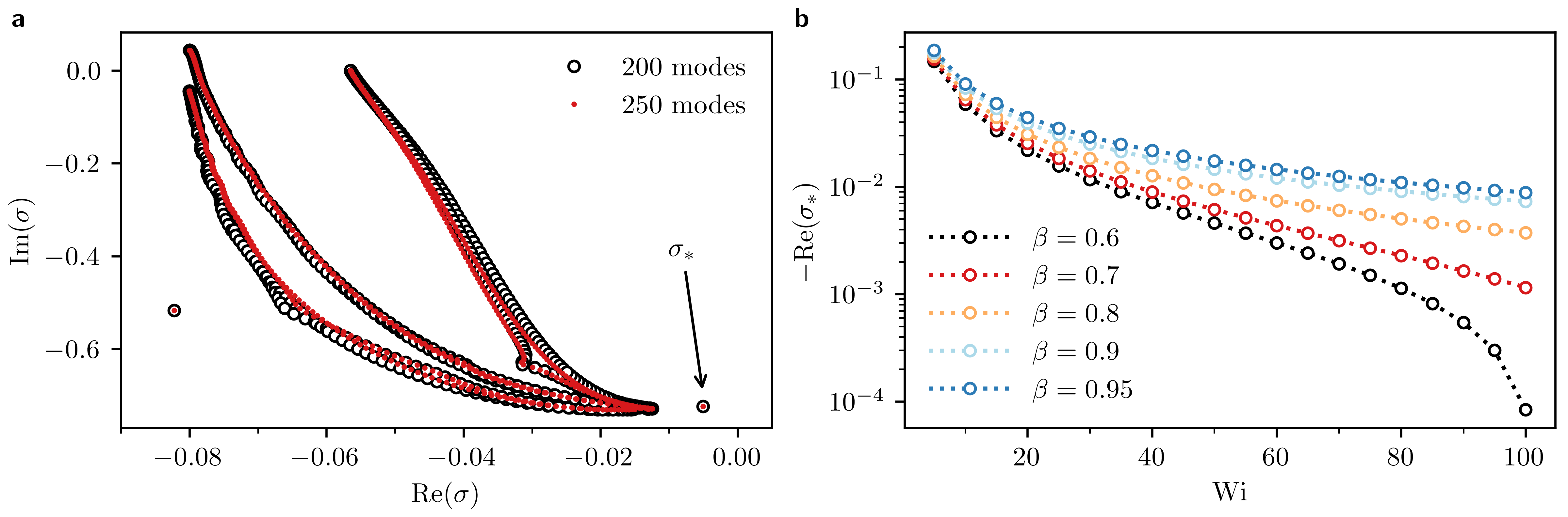
Figure S1: The results of linear stability analysis for $k=2\pi/L_{x}$. a, The eigenvalue spectrum for $\beta=0.8$ and $W\!i=80$ at two Chebyshev resolutions, showing numerical convergence. The leading eigenvalue is denoted by $\sigma_{*}$. b, The real part of the leading eigenvalue as a function of $W\!i$ for various values of $\beta$ calculated with $250$ Chebyshev modes. No linear instability is found.

Figure S2: Normalised pressure profile $p\,Re$ of the travelling wave solution for $\beta=0.8$ and $W\!i=80$. In these units, the laminar pressure gradient along the channel is $2$.

References

• CanutoΒ etΒ al. [2012] C.Β Canuto, M.Β Y.Β Hussaini, A.Β Quarteroni, A.Β ThomasΒ Jr, etΒ al.,Β Spectral methods in fluid dynamicsΒ (Springer Science & Business Media,Β 2012).
• ZhangΒ etΒ al. [2013] M.Β Zhang, I.Β Lashgari, T.Β A.Β Zaki,Β andΒ L.Β Brandt,Β J. Fluid Mech.Β 737,Β 249–279 (2013).
• KhalidΒ etΒ al. [2021] M.Β Khalid, V.Β Shankar,Β andΒ G.Β Subramanian,Β Phys. Rev. Lett.Β 127,Β 134502 (2021).
• BuzaΒ etΒ al. [2021] G.Β Buza, J.Β Page,Β andΒ R.Β R.Β Kerswell,Β arXiv:2107.06191Β  (2021).
• PooleΒ etΒ al. [2019] R.Β J.Β Poole, M.Β Davoodi,Β andΒ K.Β Zografos,Β Bull. - Br. Soc. Rheol.Β 60,Β 29 (2019).
• PanΒ etΒ al. [2013] L.Β Pan, A.Β Morozov, C.Β Wagner,Β andΒ P.Β E.Β Arratia,Β Phys. Rev. Lett.Β 110,Β 174502 (2013).