Astrometric excess noise in Gaia EDR3 and the search for X-ray binaries

Abstract

Astrometric noise ($\epsilon$) in excess of parallax and proper motion is a potential signature of orbital wobble ($\omega$) of individual components in binary star systems. The combination of X-ray selection with astrometric noise could then be a powerful tool for robustly isolating accreting binaries in large surveys. Here, we mine the Gaia EDR3 catalogue for Galactic sources with significant values of astrometric noise over the parameter space expected for known and candidate X-ray binaries (XRBs). Cross-matching our sample with the Chandra Source Catalogue returns a primary sample of $\approx$ 6,500 X-ray sources with significant $\epsilon$. X-ray detection efficiency for objects with significant $\epsilon$ is a factor of $\approx$ 4.5 times higher than in a matched control sample exhibiting low $\epsilon$. The primary sample branches off the main sequence much more than control objects in colour-mag space, and includes a higher fraction of known binaries, variables and young stellar object class types. However, values of $\epsilon$ reported in the Gaia pipeline releases so far can exceed expectations for individual XRBs with known semi-major axis size and other system parameters. It is likely that other factors (possibly attitude and modelling uncertainties, as well as source variability) currently dominate the observed excess noise in such systems. Confirmation of their nature must therefore await future Gaia releases. The full X-ray matched catalogue is released here to enable legacy follow-up.

1 Introduction

Understanding final stage binary evolution is key to tracing the life cycle of the population of interacting binaries. There has been a surge in interest in compact binaries following the discovery of gravitational wave sources (Abbott et al., 2016). But it remains unclear if and how the current LIGO/Virgo populations connects to the electromagnetically observed accreting binary sources, e.g. do they cover systematically different parameter space in mass, natal kicks, compact object spin, and evolutionary history, to name just a few (e.g. Mandel, 2016; Gandhi et al., 2020; Jonker et al., 2021; Fishbach & Kalogera, 2021)?

A key bottleneck here is the paltry number of confirmed stellar-mass black holes. There are only about 25 known stellar-mass black holes in the Milky Way with dynamical mass estimates. All of them lie in binary systems where spectroscopic radial velocity variations of the companion star have been used to confirm the presence of massive compact objects (Corral-Santana et al., 2016; Tetarenko et al., 2016a). By contrast, the Galaxy is expected to host anywhere between $\sim$ 10³–10⁸ stellar-mass black holes in binary systems (e.g. Pfahl et al., 2003; Tetarenko et al., 2016b). This population should be dominated by non-accreting systems and incipient black hole X-ray binaries (BHXBs) with only a handful of recent well studied systems (Thompson et al., 2019; Tetarenko et al., 2016b; Rivinius et al., 2020). An interesting recent highlight in this field was LB-1, with a proposed $M_{\rm BH}$ = 70 M_⊙ (Liu et al., 2019). Though now believed to be much lighter (e.g. Eldridge et al., 2020; El-Badry & Quataert, 2021; Abdul-Masih et al., 2020; Irrgang et al., 2020), its discovery accelerated efforts to understand the space density of massive quiescent BHXBs. Other examples include the report of a putative black hole in V723 Mon (Jayasinghe et al., 2021), in the triple system HR 6819 (Rivinius et al., 2020), and in the open cluster NGC 1850 (Saracino et al., 2021), though the latter two also remains controversial (Bodensteiner et al., 2020; El-Badry & Burdge, 2021). Clearly, more efforts are needed to enhance this population if we are to properly constrain final stage binary evolution.

The exquisite astrometric precision now being enabled by missions such as Gaia opens up a new window on such studies. In particular, orbital motion of the companion star in a binary system will result in ‘astrometric orbital wobble ($\omega$)’, over and above the parallax and proper motion locus determined for single-object astrometry. This can manifest as an ‘astrometric excess noise ($\epsilon$)’, one of the parameters reported in the early data release Gaia Collaboration et al. 2018, 2021). $\epsilon$ is defined as the excess uncertainty that must be added in quadrature to obtain a statistically acceptable astrometric solution (Gaia Collaboration et al., 2018; Lindegren et al., 2012).. In the early data releases, $\epsilon$ includes instrument and attitude modelling errors that are statistically significant and could result in large values of $\epsilon$. Thus, a detailed investigation of $\epsilon$-based selection is warranted, and this is what we carry out herein.

Several recent theoretical works have highlighted the feasibility of large surveys, including astrometric missions (Gould & Salim, 2002; Barstow et al., 2014; Breivik et al., 2017; Mashian & Loeb, 2017; Yalinewich et al., 2018; Andrews et al., 2019; Chawla et al., 2021) and microlensing searches (Masuda & Hotokezaka, 2019; Wiktorowicz et al., 2021), to uncover large new populations of black holes in binary orbits. Massive spectroscopic surveys are also beginning to probe this territory through brute force blind searches for radial velocity variations characteristic of massive compact objects (Yi et al., 2019; Wiktorowicz et al., 2020; Price-Whelan et al., 2020). Furthermore, large multiwavelength surveys such as eROSITA in X-rays (Merloni et al., 2012) and ngVLA in the radio (Maccarone et al., 2018) will be instrumental in confirming the nature of newly identified candidates, and characterising their physical properties (e.g. with the Rubin Observatory; Johnson et al. 2019). Thus, there are enormous synergies waiting to be explored in this field. We exploit one such synergy of astrometric noise combined with X-ray photometry here.

2 Astrometric wobble and excess noise

Astrometric wobble ($\omega$) is defined here simply as the maximal projected half angle swept by the companion star over its orbit, if the observed flux is dominated by the companion star.

$$\omega=\frac{a_{2}}{d}$$ (1)

where $a_{2}$ is the semi-major axis of the companion and $d$ the source distance. For the typical physical parameters and distances of known XRBs, $\omega$ is expected to lie in the range of $\sim$ 0.01–1.0 mas (e.g. Gandhi et al. 2019). For simplicity, a circular orbit is assumed in these approximate estimates, since interacting binaries (our core targets of interest) are expected to circularise rapidly. While this is not the case for the (often highly) eccentric Be X-ray systems (see e.g. Reig 2011), virtually all known Be X-ray sources have neutron star (NS) compact objects, so the astrometric wobble of the (much) more massive Be donor is expected to be very small. The assumption of the flux being dominaed by the companion should be mostly true in quiescent, non-accreting, and high-mass XRBs, though the accreting primary in low-mass XRBs can contribute a few tens of per cent of the total flux (which would result in a smaller apparent centre-of-light wobble).

Astrometric noise $\epsilon$ represents an additional intrinsic scatter term in the Gaia pipeline astrometric solution, where it is expressed in angular units of mas. This is the value that needs to be added in quadrature to the formal statistical uncertainties in order to make the single-object solution statistically acceptable, effectively making the reduced sum-of-squared-weighted-residuals equal unity (Lindegren et al., 2012).

Since $\omega$ represents a deviation from the nominal parallax locus, it is equivalent to an excess scatter term, and is thus conceptually similar to $\epsilon$, if no other noise terms contribute. In such a case, the expectation value of $\epsilon$ should approximate $\hat{\omega}$ = $\omega$/$\sqrt{2}$ in the limit of perfect orbital sampling. However, in early Gaia releases, $\epsilon$ absorbs instrumental as well as attitude modelling errors that are likely to be statistically significant. The excess noise terms are globally adjusted to match the weighted sum of residuals to the number of degrees of freedom (Lindegren et al., 2018), so there could be some potential degeneracy between the magnitudes of the noise terms, and they need not scale directly and strictly with $\omega$ for individual objects. Thus, caution is needed in their interpretation (Lindegren et al., 2012; Luri et al., 2018; Gaia Collaboration et al., 2018, 2021), and other supporting evidence should be leveraged as we describe in the following section.

As an aside, astrometric perturbations to single-source pipeline fits are quantified in the Gaia pipeline in a variety of ways. In addition to $\epsilon$, the Gaia data releases include a parameter statistic termed RUWE (Renormalised Unit Weight Error). This is equivalent to a goodness-of-fit renormalised to 1 after accounting for systematic pipeline issues including a degrees-of-freedom bug as well as fit variations based upon colour (Lindegren et al., 2018). Significantly higher values than 1 can be signposts of intrinsic source complexity. RUWE selection and $\epsilon$ selection are thus complementary to each other, with each having its pros and cons (e.g., Belokurov et al., 2020; Penoyre et al., 2020). Here, we are focusing on $\epsilon$ due to its straightforward interpretation as a characteristic projected binary size. Another advantage is that the Gaia pipeline quantifies and reports the significance of $\epsilon$, unlike RUWE. The Gaia team have explored the regime where care is needed with $\epsilon$ selection and we have adopted their recommendations (see following section). In any case, the aforementioned pipeline systematic issues will, at worst, result in an underestimate of $\epsilon$, so our selection is likely somewhat conservative.

3 Sample selection

3.1 Mining Gaia

With the reference parameter range of known XRBs discussed above as a starting ansatz, we used the following selection criteria. The Gaia EDR3 archive reports a significance value of $\geq$ 2 when $\epsilon$ is considered significant. At mags $G$ $<$ 13, there are systematic calibration uncertainties in EDR3, resulting in artificially enhanced values of $\epsilon$ (Gaia Collaboration et al., 2021; Lindegren et al., 2021a). Conversely, statistical uncertainties dominate near the faint mag limit of $G$ = 21. We thus restricted our mag range to 13 $<$ $G$ $<$ 20. This encompasses the median mag of BHXBs with five-parameter astrometric solutions measured in DR2 ($G$ $\approx$ 17.4; Gandhi et al. 2019), and should probe the mag range that is currently most robust to the aforementioned uncertainties. A distance range of 0.1–10 kpc was examined, requiring a significant parallax (distance) measurement in order to try and assess the nature of the source population, as discussed in the following section. A minimum threshold on the number of visibility periods is used to ensure adequate sampling in time in the astrometric fit. The corresponding EDR3 ADQL (Osuna et al., 2008) query for our primary sample over the full sky is:  

SELECT *
FROM gaiaedr3.gaia_source
WHERE (astrometric_excess_noise >= 0.01)    AND
   (astrometric_excess_noise_sig >= 2)    AND
   (parallax $<$ 10.) AND (parallax $>$ 0.1) AND
   (parallax_over_error $>$ 5) AND    (visibility_periods_used $>$ 10) AND
   (phot_g_mean_mag $>$ 13) AND
   (phot_g_mean_mag $<$ 20).  

We also defined a control sample for cross-comparison. The EDR3 ADQL query for this control sample is identical to the above except for the excess noise selection criterion, because this is our main parameter of interest. We thus modify the relevant portion of the query with a complementary criterion, as follows:

(astrometric_excess_noise < 0.01).  

Good astrometric fits require sources to be free from confusion and blending with close neighbours. Therefore, we next excluded all objects with any detected EDR3 near-neighbours. A radius of 2″ was adopted for our near-neighbour threshold, given that the nominal Gaia point spread function is concentrated well within 1 arcsec. This mitigates crowding issues impacting astrometry in dense regions of the Galactic plane.

The final parallaxes that we report have been corrected for zero-point astrometric offsets, as recommended by the Gaia team (Lindegren et al., 2021b); these were calculated from the mean photometeric $G$ band magnitude (phot_g_mean_mag), $\nu_{eff}$ (nu_eff_used_in_astrometry), the pseudocolour (pseudocolour), the ecliptic latitude (ecl_lat) and the number of astrometric parameters solved (astrometric_params_solved). The resultant zeropoint offsets, calculated as described in Lindegren et al. (2021b), were then subtracted from the raw parallaxes reported by EDR3 pipeline.

3.2 Cross-match with X-rays

X-ray activity is a key signature of accretion in binaries. Quiescent BHXBs are expected to exhibit low-level accretion activity, with typical luminosities of up to $L_{\rm X}$ $\sim$ 10^30-32 erg s^-1, and NSXBs in quiescence can be even more luminous, on average (e.g. Reynolds & Miller, 2011). However, detection of X-rays by itself is not unambiguous proof of the presence of an interacting binary, with other possibilities including magnetically active stars (e.g. Güdel, 2004), colliding winds (e.g. Pittard & Dawson, 2018), and activity in young stellar objects (e.g. Feigelson & Montmerle, 1999). So care will be necessary when making final inferences.

We queried the Chandra Source Catalogue (CSC; Evans et al. 2010) for overlap with our sample. This is still one of the largest, and most sensitive, public databases in terms of broadband X-ray sky coverage, delivering exquisite spatial resolution ($\mathrel{\hbox{\hbox to0.0pt{\hbox{\lower 4.0pt\hbox{$\sim$}}\hss}\hbox{$<$}}}$ 1″ on axis). High precision centroiding is critically important in crowded regions such as the Galactic plane, along which many of our sources will fall. The latest data release, CSC2.0 (Evans et al., 2020), covers approximately 550 deg² (1.3 %) of the sky down to a point source sensitivity limit of 5 counts. Assuming a reference spectrum of an accreting source characterised by an X-ray power-law with slope $\Gamma$ = 2, this sensitivity corresponds to a 0.5–7 keV flux limit $F_{\rm X}$ of 6 $\times$ 10^-15 erg cm^-2 s^-1 at the median CSC2 exposure time of 12 ks. This is an approximation based upon the latest response function and assuming a line-of-sight column density $N_{\rm H}$ = 5 $\times$ 10²¹ cm^-2, not atypical out to distances of a few kpc in the Galactic plane. The Chandra soft energy response has been degrading with time so it is likely that older observations were more sensitive, on average. Taking the above flux limit as a baseline for comparison, CSC2 should be able to detect XRBs out to a distance $d$ with luminosity greater than

$$L_{\rm X-ray}>7\times 10^{29}\left(\frac{d}{1\,\rm{kpc}}\right)^{2}\,{\rm erg\,s^{-1}\,\,\,[0.5-7\,keV]}.$$ (2)

A maximal optical/X-ray cross-matching offset of 1$\arcsec$ was adopted, after back-tracing the Gaia 2016 reference epoch coordinates to 2000 using their EDR3 proper motions. We used the broad band (0.5–7 keV) fluxes listed under the flux_aper_b parameter. In a small fraction of cases, a non-zero value of the wide-band 0.1–10 keV flux_aper_w parameter is instead found, and this was converted to an equivalent broad-band flux. There is also a small fraction ($\sim$ 10%) of sources where a flux measurement fails completely. We nevertheless retained these sources for some of the statistical analysis presented later, as their exclusion did not significantly impact our inferences.

4 Results

Selection basis	Primary	Control
Gaia EDR3	18,682,537	96,044,222
Gaia + Chandra	6,569	7,412

Table 1: Sample selection statistics

Table 1 lists the number of sources selected under various criteria. Our Gaia/EDR3 mining resulted in over 18 million sources selected in the ‘primary’ sample. These are sources with significant astrometric excess noise and no close neighbours. The corresponding ‘control’ sample was much larger as expected, approaching 100 million sources. The peak mags for primary and control are, respectively, $G$ = 15.7 and $G^{\prime}$ = 16.4. Here, and hereafter, a prime (^′) superscript refers to the control sample. The control sample objects tend to lie farther than primary sources, with mean distances of $\langle d^{\prime}\rangle$ = 1.9 kpc and $\langle d\rangle$ = 1.2 kpc, respectively, and a standard deviation of 1.0 kpc for both. Here, we use parallax inversion $d$ (kpc) = $\frac{1}{\pi}$, where $\pi$ is the zero-point-corrected EDR3 parallax in mas. Parallax inversion should be a fair estimator of the distance if $\pi$ is well constrained, and certainly reasonable for population-wide comparisons.

With this selection, the full Gaia-only selected sample ends up with a $\epsilon$ value distribution peaking near $\epsilon$ $\approx$ 0.25 mas, but with an extended tail to $\approx$ 17 mas. By contrast, the vast majority (99.9 %) of control sample objects have $\epsilon$^′ = 0 mas. The above differences in characteristic brightness and distances between the primary and the control samples likely reflects the fact that detecting significant intrinsic perturbations to static single-object astrometric fits is simply more effective when sources are nearer and/or brighter.

The Chandra cross-match resulted in over 6,500 X-ray detected sources in the primary sample and about 7,400 in control. Importantly, this translates into a very significant difference in terms of population fractions. The fraction of X-ray detected sources ($f_{X}$) = 3.52 ($\pm$ 0.04) ${}^{\text{o}}\mkern-5.0mu/\mkern-3.0mu_{\text{ooo}}$ for the primary sample. This is a factor of $\approx$ 4.5 times higher than that in control, $f_{X}^{\prime}$ = 0.77 ($\pm$ 0.01 ${}^{\text{o}}\mkern-5.0mu/\mkern-3.0mu_{\text{ooo}}$), a difference that holds true across all mags and much of distance range probed. This is illustrated in Fig. 1, showing $f_{X}$ split as a function of distance, with $f_{X}$ being consistently higher than $f_{X}^{\prime}$ out to about 2 kpc, reflecting the drop in the joint X-ray detection and astrometric selection efficiencies with distance. The full catalogues are available through CDS.

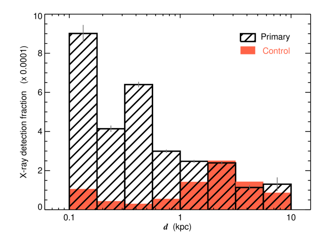
Figure 1: X-ray detection fraction ($f_{X}$) as a function of source distance $d$. $f_{X}$ is consistently larger in the primary sample (black hatched) than in control ($f_{X}^{\prime}$; red), out to $d$ $\approx$ 2 kpc. The uncertainties show Poisson sampling errors on the primary sample.

Fig. 2 shows the Gaia colour–mag diagram (CMD) for the X-ray cross-matched samples. EDR3 does not report extinction and reddening values, so we extracted and applied these from DR2, where available. We advise caution that these saturate around $A_{\rm G}$ $\approx$ 3 mag and $E(B_{\rm p}-R_{\rm p})$ $\approx$ 1.5 mag (Andrae et al., 2018); thus, these corrections are underestimated for many individual systems. Nevertheless, canonical features such as the main sequence (MS) and the giant branch immediately stand out. In addition, a clump redder than the MS at relatively faint levels is apparent, corresponding to the expected locus of young stellar objects (YSOs), or to the less-understood population of sub-subgiants (e.g. Geller et al., 2017).

There are some important differences apparent between the two samples. The primary sample extends substantially deeper into the evolved/reddened branch, off the MS, than the control sample. Specifically, the mean $\langle$$B_{\rm p}$ – $R_{\rm p}$$\rangle$ colour is $\approx$ 0.3 mag redder in primary than control. The reddest source has a $B_{\rm p}$ – $R_{\rm p}$ colour almost 2 mag larger than in control. All objects plotted in the CMD have reddening and extinction corrections applied, so underestimates in these corrections likely only play a partial role in explaining these differences. Instead, the larger scatter of primary sample sources suggests that $\epsilon$-selection preferentially picks up objects with a wide spread of evolutionary phases and source classes.

Source type assignments are denoted on the diagram, where available. Information regarding known object classifications was collated using a simple cross-match with SIMBAD. The ‘main_type’ of the closest association within a threshold distance of 1 arcsec of the Gaia coordinates was extracted. These were then grouped into a few broad categories for summarisation. The complete list of classes and categories can be found in the Appendix. Sky coverage of classifications is patchy and highly incomplete. But this exercise is solely meant to provide first insight into the putative nature of our selected population.

About 1% of objects from the full Gaia-only selection have a documented classification in SIMBAD, albeit being in uncertain in many cases. Since object type determination may be implicitly distance or mag dependent, a fair comparison was carried out by distance-matching the two samples. For this, we randomly selected one control sample source for every primary sample source, to within a distance threshold of 0.05 kpc, so that the distribution of distances becomes statistically indistinguishable. The resultant distance-matched sub-sample comprised about 8 million objects, and results on the relative comparison are shown in Fig. 3 and Table 2.

The fraction of objects with known classifications is $\approx$ 0.9% (control) and 1.2% (primary). By contrast, the fraction of known binaries in the primary sample outnumbers those in control by more than a factor of 2. These include non-interacting systems as well as interacting binaries such as XRBs and CVs. Three other source types are highlighted here – variables, emission line objects, and young stellar objects – as these will be relevant to the Discussion later. In all these cases, again, the corresponding fraction of systems in the primary sample is more than a factor of 2 larger than control.

In X-rays, the matched sample luminosity distributions are qualitatively similar, peaking close to $\langle{\rm log}[L_{\rm X}\,/\,{\rm erg}\,{\rm s}^{-1}]\rangle$ = 29.5, with a high tail extending beyond a peak of $L_{\rm X}$ $\approx$ 10³² erg s^-1.

SIMBAD object type distributions Class $f_{\rm Primary}$ $f^{{}^{\prime}}_{\rm Control}$ 10^-4 10^-4 All 118.7 $\pm$ 0.4 87.8 $\pm$ 0.3 Binary (B) 12.0 $\pm$ 0.1 5.8 $\pm$ 0.1 Variable (V) 18.7 $\pm$ 0.1 8.7 $\pm$ 0.1 YSO (Y) 6.9 $\pm$ 0.1 3.0 $\pm$ 0.1 Emission line (m) 0.54 $\pm$ 0.02 0.22 $\pm$ 0.02

Table 2: Fractions of object types from SIMBAD, split into a few of the key broad categories. These refer to the distance-matched samples for fair comparison, and shown pictorially in Fig. 3. The letter in parentheses is that used in the CMD (Fig. 2) to depict them.

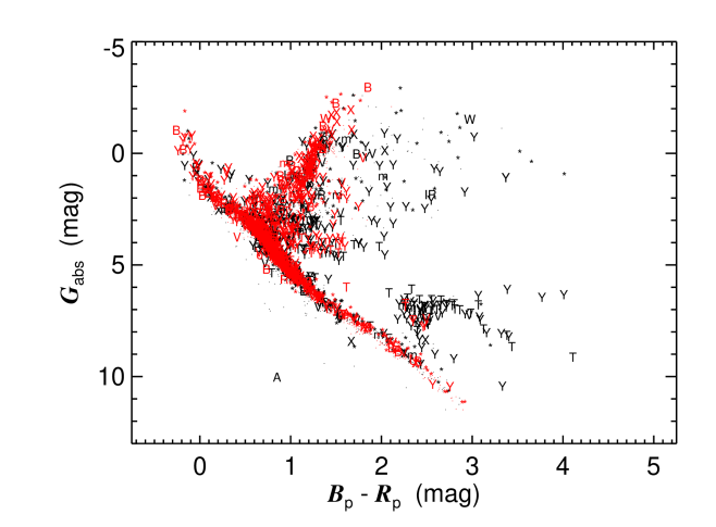
Figure 2: Gaia colour–mag diagram for the X-ray cross-matched samples (black: primary sample; red: control sample). Individual object types from SIMBAD are denoted, with a few key types as follows. ‘B’: Binary, ‘V’: Variable, ‘Y’: YSO, ‘T’: TTau, ‘X’: X-ray source, ‘W’: Wolf-Rayet, ‘m’: Emission line source. Objects with a more normal stellar classification (e.g. ‘Star’) are denoted by an asterisk, and those without an archival class are denoted as dots.

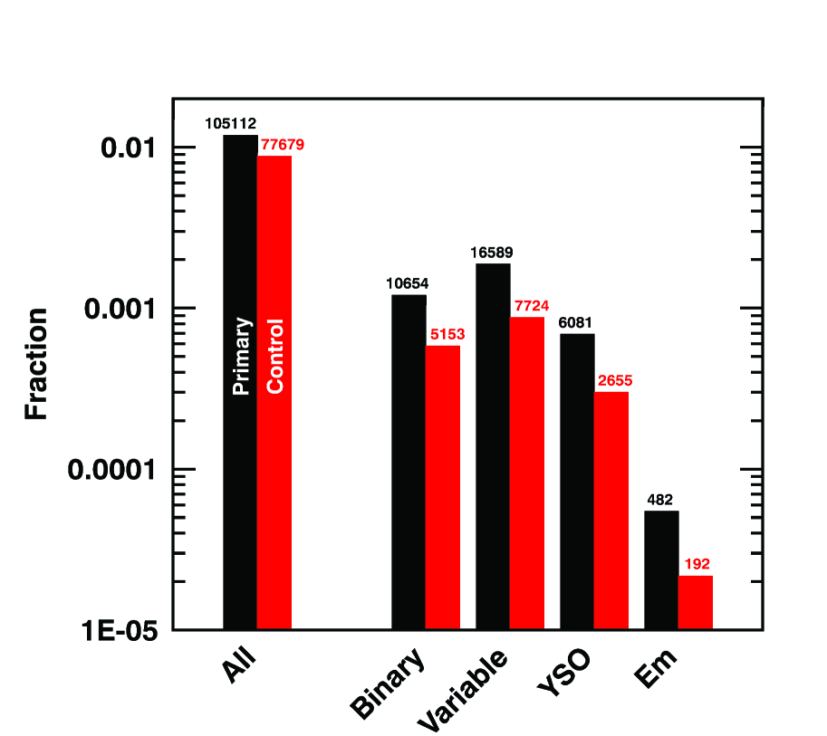
Figure 3: Distribution of object classes cross-matched with SIMBAD. Here, distance-matching has been applied for a fair cross-comparison between primary and control. Only a few broad categories are shown (for the full list, we refer the reader to the Appendix). Above each histogram bar, the number of objects in that bin is stated.

5 Discussion

We began this study with the aim of searching for previously unidentified or ill characterised, putative interacting binaries. What is the nature of our sample, and are we likely to have detected robust accreting binary candidates?

Our prime selection criterion is astrometry-based (choosing a sample of Galactic point sources with significant astrometric excess noise; $\epsilon$), which was then refined using photometric properties (X-ray detection). The nature of $\epsilon$ selection and its veracity still remain unclear in the early Gaia data releases, and the individual astrometric measurements have not yet been released. This is why we chose to explore the influence of $\epsilon$ selection in a controlled manner and in a relative sense between two closely similar samples. The most significant highlights of our selection are:

1. The X-ray detection fraction with Chandra in our primary sample is significantly higher, about 5 times more, than control (Fig. 1, Table 1). This is true across all (optical) mags and out to distances of $\approx$ 2 kpc where the samples become comparable presumably due to the currently limited X-ray sensitivity and a decreasing $\epsilon$ measurement efficacy with distance.

2. Sources with significant $\epsilon$ lie closer to us than the control sample ($\langle d^{\prime}\rangle$ = 1.9 kpc vs. $\langle d\rangle$ = 1.2 kpc), again, presumably due to the fact that higher order astrometric signatures are easier to measure for nearer (brighter) objects.

3. Occupancy in colour–mag space across the CMD differs between the two samples, with the primary sample occupying the regime of redder/more evolved colours (Fig. 2).

4. We find a higher fraction of objects with current classified types as binaries, variables, emission line sources and young stellar objects in the primary sample (Fig. 3 and Table 2).

While any one of the above differences may be attributable to selection effects or systematic uncertainties in astrometric fitting, such explanations do not suffice when considering the above differences cumulatively. In particular, systematic effects in any one mission or wavelength (e.g. Gaia) would not obviously be expected to result in differences at other wavelengths (Chandra) or in other catalogues (SIMBAD spectroscopic classifications). Thus, the above differences suggest that $\epsilon$ selection is effective in picking up sources with intrinsically distinct properties, on average.

Our X-ray selection is able to probe down to the level where quiescent emission from XRBs is detectable ($L_{\rm X}$ $\mathrel{\hbox{\hbox to0.0pt{\hbox{\lower 4.0pt\hbox{$\sim$}}\hss}\hbox{$>$}}}$ 10^28-32 erg s^-1). Accreting XRBs often comprise evolved donor stars undergoing Roche-lobe-overflow mass transfer that generates X-rays, also encouragingly consistent with the larger fraction of objects located off the main sequence in the CMD. All these facts are consistent with the presence of new quiescent accreting binaries amongst our primary sample. But this is not unambiguous.

Regarding known source classifications, emission line objects with limited prior observational follow-up could also be hiding accreting systems with viscous disc heating or with irradiation powering line emission. Variability is an additional characteristic property of quiescent accretion (e.g. Zurita et al. 2003). Variables, however, cover a broad range of source classes, and we cannot rule out the possibility that these may include single active stars where the variability causes systematic perturbations to the individual astrometric measurements, resulting in artificially boosted $\epsilon$. The presence of YSOs amongst our selected objects may appear surprising at first. But this could be a simple consequence of the fact that YSOs have a high multiplicity that decreases with evolutionary phase and scales with mass (e.g. Pomohaci et al., 2019). Consequently, younger YSOs in our primary sample could well include a high fraction of binaries showing significant $\epsilon$. YSOs are known to be variable in flux, and are also known to be X-ray sources (Feigelson & Montmerle, 1999). Thus, there are multiple reasons why our selection picks up YSOs.

A final systematic issue to be aware of is that of crowding. While we have attempted to mitigate this issue by excluding close Gaia neighbours, it is not inconceivable that other contaminants (those below the Gaia pipeline detection threshold) may be impacting source astrometrics in regions such as star and globular clusters. Partially resolved double stars could also introduce biases in single-star astrometric solutions. Fabricius et al. (2021) suggest cuts on the Image Parameter Determination (ipd) factors ipd_frac_multi_peak $>$2 OR ipd_gof_harmonic_amplitude $>$ 0.1, in order to flag solutions with multiple peaks and asymmetries. Using these criteria would flag 22 % of our primary sample as being potentially impacted due to the presence of partially resolved doubles. While we have not included blanket additional cuts to remove such objects (since they could include objects of inherent interest for our selection), any inference regarding the nature of objects in particularly crowded regions should be treated carefully. The bulk of the sample is not impacted by such ipd flags.

Radial velocity curves would be needed to confirm the nature of these various object types, to test for binarity and to measure their system characteristics, while deeper X-ray and radio data could establish the nature of high-energy activity. Current model predictions suggest that Gaia ought to detect several hundreds to thousands of BHs in binary systems (e.g. Yamaguchi et al., 2018; Breivik et al., 2017; Chawla et al., 2021), with a preference for more precise measurements of longer period systems (Andrews et al., 2019). Methods have also been proposed to detect non-interacting systems with MS companions (Shahaf et al., 2019) with Gaia. Quiescently accreting systems (of the kind that we have discussed herein) will likely be a fraction of these, but will be the ‘low hanging fruit’ that are likely to be the easiest ones to find, follow up and confirm.

The mean value of excess noise across our primary X-ray detected sample, $\langle\epsilon\rangle$ = 0.44${}_{-0.26}^{+0.64}$ mas at the mean distance of 0.9 kpc, translates to an expected orbital semi-major axis $a_{2}$ $\approx$ 0.5 AU if interpreted as the maximal astrometric orbital perturbation of a binary projected onto the sky. Any binary systems with these characteristic sizes would be akin to long period systems such as the long-period BHXB GRS 1915+105 (Casares & Jonker, 2014) or the cataclysmic variable T CrB (Fekel et al., 2000). The most compact systems amongst our sample, however, extend down to $a_{2}$ $\approx$ 0.009 AU, easily compatible with the regime of short-period accreting binaries (e.g. Casares & Jonker, 2014). This is illustrated in Fig. 4, where the estimated values of $a_{2}$ are plotted for our full primary sample of $\approx$ 6,500 objects as a function of $\epsilon$, and compared with $a_{2}$ estimates for several known BHXBs which cover similar parameter space.

These are simple first-order $a_{2}$ estimates, and the aforementioned caveats (assumption of a circular orbit, well-sampled astrometry, and no radiative contribution from the accreting primary component) should be kept in mind while drawing any detailed inferences on individual systems. Additional caution is also warranted because the current magnitudes of $\epsilon$ actually overestimate expectations in a few known systems. Examples include Her X–1 ($\epsilon$ = 0.09 $\pm$ 0.01 mas as compared to $\hat{\omega}$ = 0.002 mas) and V404 Cyg ($\epsilon$ = 0.41 $\pm$ 0.08 mas as opposed to $\hat{\omega}$ = 0.04 mas). One possible systematic issue here may be photometric variability. V404 Cyg underwent a dramatic outburst in 2015, displaying prolific flux changes by up to 7 mag over a period of a few weeks (e.g., Kimura et al., 2016; Gandhi et al., 2016). But given that the outburst of V404 Cyg was relatively brief, it is difficult to see how such changes could dominate the astrometric solution determined over the full EDR3 observation period. Her X–1 is an eclipsing system with known orbital and superorbital flux modulations on characteristic timescales of about 2 days and 1 month, respectively (Jurua et al., 2011). Such variations could potentially introduce systematic variations in the epochwise astrometric uncertainties. A second systematic issue may come down to an underestimate of the pipeline parallax uncertainties, as suggested by El-Badry et al. (2021); this would artificially boost $\epsilon$, though the root cause of such an underestimate of the parallax uncertainties remains unclear. Finally, attitude errors could also bias the astrometric solutions; attitude errors are time-dependent and have been globally adjusted for weighted residuals in released pipeline solutions (Lindegren et al., 2012; Lindegren et al., 2018, 2021a). The individual astrometric measurements, not yet available, will be needed to clarify the underlying cause of the mismatch between expectations and the pipeline reported measurements.

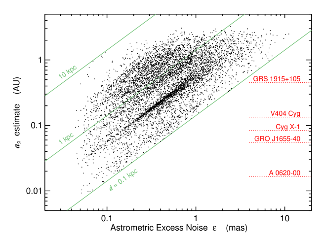
Figure 4: Astrometric excess noise ($\epsilon$) vs. putative binary companion star semi-major axis $a_{2}$. The latter is computed from Eq. 1 and assuming that $\epsilon$ is an estimator of $\omega$/$\sqrt{2}$ in the limit of perfect sampling. See text for details and caveats. Three loci covering a range of distances are plotted in green. Known or estimated values of $a_{2}$ for five known BHXBs are denoted by the red dotted lines. The clustering of objects near the middle of the figure is likely an artefact of dense X-ray sampling of the Orion star-forming region at $d$ $\approx$ 0.4 kpc.

6 Conclusions

We have explored the statistics and nature of objects found using astrometric excess noise selection in Gaia EDR3. Our initial aim was to identify candidate accreting systems. But a variety of tests carried out in a controlled fashion demonstrate that excess noise selection is effective in identifying a diverse range of active source classes. X-ray cross-matching is used to refine the selection to identify putative quiescent interacting binaries, variables, emission line sources and young stellar objects, amongst others.

Our astrometric selection encompasses the parameter space expected for orbital wobble in accreting binaries. But caution is needed when interpreting the current reported values of excess noise, especially when $\epsilon$ is small (well below 1 mas); systematic effects including attitude errors, partially resolved double stars, and source variability likely contaminate our selection to a certain extent at present. Full astrometric solutions in future data releases will help to understand the selection function more quantitatively. Nevertheless, our sample is unlikely to be dominated by such systematics, because of the addition of independent X-ray constraints. Upcoming all-sky X-ray followup from eROSITA will also provide a treasure trove of other candidate active systems enhancing the sample that we present here (Merloni et al., 2012). Similarly, in the future, Galactic plane follow-up with the ngVLA should accomplish the same in the radio (Maccarone et al., 2018).

This is a first detailed attempt to utilise astrometric wobble to search for robust binary candidates over the full sky. Our sample is not meant to be complete in any physical sense yet; rather, this is a first attempt to pick the ‘low hanging’ fruit in EDR3 astrometric noise selection of accreting binaries. We release our primary source sample to enable multiwavelength follow-up and characterisation of individual systems.

Data availability

All of the multiwavelength catalogues utilised herein (Gaia, Chandra) are publicly available. Our final extracted catalogue will also be available through Vizier/CDS upon publication of this manuscript.

Appendix A Full catalogue

A few example catalogue entries are listed in Table 3. The full table will be available through CDS.

Primary sample catalogue
RA_(EDR3) Dec_(EDR3) $G$ $d$ $\epsilon$ $F_{\rm X}$ $\Delta$ Class Source ID deg deg mag kpc mas 10^-15 erg s^-1 cm^{-2 ′′} 39.059798817  +59.692402581 15.20 1.43 $\pm$ 0.11 0.36 $\pm$ 0.01 4.4 0.4 – – 95.685591321    –0.345659073 17.47 1.38 $\pm$ 0.24 0.37 $\pm$ 0.17 17 0.1 HMXB 1A 0620–00 53.243901052   –27.835515446 17.46 0.34 $\pm$ 0.02 1.22 $\pm$ 0.02 0.11 0.3 Galaxy^† 2MASS J03325851–2750079 254.457539283   +35.342322461 13.62 7.07 $\pm$ 1.04 0.09 $\pm$ 0.01 56450 0.7 LMXB HZ Her

Table 3: ICRS coordinates from the default EDR3 reference epoch of 2016 are listed. The distance $d$ here is based on parallax inversion and is corrected for zeropoint offset. $F_{\rm X}$ denotes the Chandra CSC2 broadband flux (0.5–7 keV). $\Delta$ denotes the coordinate offset between Gaia and Chandra. The ‘Class’ and ‘Source ID’ are those reported by SIMBAD, as of Oct 2021. A portion of the catalogue is shown here for reference, with the full catalogue available through CDS. ^†The ‘Galaxy’ in row 3 is likely an incorrect SIMBAD class.

Appendix B SIMBAD Object Classifications and Assigned Codes

Tables B1 and B2 list the individual source types (the main_type from SIMBAD) together with the corresponding assigned short code denoting the broad source category used in the Results, Discussion and some of the figures in the main paper.

We caution that a small fraction of objects ($\sim$ 1 %) have unexpected classifications (e.g. extragalactic sources, extended objects such as planetary nebulae [PN], and even candidate planets). Examining the apparent extragalactic sources suggests prior source types are probably in error (either simple transcribing errors between SIMBAD and published work, or source confusion). All of them have significant positive parallax measurements consistent with being Galactic objects. The reason that a few PN lie in our primary sample remains unclear; e.g. whether or not the extended nebular emission introduces artificial astrometric uncertainties. Such objects should obviously be treated with caution; but given their small numbers, they will not bias any of our statistical inferences.

Object classifications from SIMBAD
Class Assigned Code Unknown multiple_object * * AGB* * BlueSG* * C* * Candidate_AGB* * Candidate_HB* * Candidate_Hsd * Candidate_RGB* * Candidate_RSG* * Candidate_S* * Candidate_SN* * Candidate_brownD* * Candidate_low-mass* * Candidate_post-AGB* * HB* * PM* * Pec* * RGB* * RedSG* * S* * Star * brownD* * low-mass* * post-AGB* * AGN A AGN_Candidate A Assoc* A BYDra B Candidate_CV* B Candidate_EB* B Candidate_HMXB B Candidate_XB* B CataclyV* B EB* B HMXB B LMXB B Nova B RSCVn B RotV*alf2CVn B SB* B Symbiotic* B XB B BlueStraggler BlueStraggler Candidate_** C Candidate_BSS C Candidate_C* C Candidate_Pec* C Cl* C ClG C Compact_Gr_G C DkNeb D EmG E FIR F HH H HII H IR IR MIR M MolCld M NIR N OH/IR O Pulsar P QSO Q QSO_Candidate Q Radio(mm) R Radio(sub-mm) R RadioG R RfNeb R Radio Radio

Table 4: Object classifications and assigned codes.

Object classifications from SIMBAD
Class Assigned Code Seyfert S Seyfert_1 S Candidate_TTau* T TTau* T UV UV Candidate_Cepheid V Candidate_LP* V Candidate_Mi* V Candidate_RRLyr V Cepheid V EllipVar V Erupt*RCrB V Eruptive* V HV* V HVCld V Irregular_V* V LPV* V Mira V Orion_V* V PulsV* V PulsV*RVTau V PulsV*WVir V PulsV*delSct V RRLyr V RotV* V Transient V V* V V*? V deltaCep V gammaDor V pulsV*SX V Candidate_WD* WD WD* WD WR* WD X X Candidate_YSO Y YSO Y denseCore d gamma g Ae* m Be* m Candidate_Ae* m Candidate_Be* m Em* m EmObj m BLLac o Galaxy o GinCl o GinGroup o GinPair o GlCl? o GroupG o PN o PN? o Planet o Planet? o HotSubdwarf sd

Table 5: Continuation of object classifications.

References

- Abbott et al. (2016) Abbott B. P., et al., 2016, Phys. Rev. Lett., 116, 061102
- Abdul-Masih et al. (2020) Abdul-Masih M., et al., 2020, Nature, 580, E11
- Andrae et al. (2018) Andrae R., et al., 2018, A&A, 616, A8
- Andrews et al. (2019) Andrews J. J., Breivik K., Chatterjee S., 2019, ApJ, 886, 68
- Barstow et al. (2014) Barstow M. A., et al., 2014, arXiv e-prints, p. arXiv:1407.6163
- Belokurov et al. (2020) Belokurov V., et al., 2020, MNRAS, 496, 1922
- Bodensteiner et al. (2020) Bodensteiner J., et al., 2020, A&A, 641, A43
- Breivik et al. (2017) Breivik K., Chatterjee S., Larson S. L., 2017, ApJ, 850, L13
- Casares & Jonker (2014) Casares J., Jonker P. G., 2014, Space Sci. Rev., 183, 223
- Chawla et al. (2021) Chawla C., Chatterjee S., Breivik K., Krishna Moorthy C., Andrews J. J., Sanderson R. E., 2021, arXiv e-prints, p. arXiv:2110.05979
- Corral-Santana et al. (2016) Corral-Santana J. M., Casares J., Muñoz-Darias T., Bauer F. E., Martínez-Pais I. G., Russell D. M., 2016, A&A, 587, A61
- El-Badry & Burdge (2021) El-Badry K., Burdge K., 2021, arXiv e-prints, p. arXiv:2111.07925
- El-Badry & Quataert (2021) El-Badry K., Quataert E., 2021, MNRAS, 502, 3436
- El-Badry et al. (2021) El-Badry K., Rix H.-W., Heintz T. M., 2021, MNRAS, 506, 2269
- Eldridge et al. (2020) Eldridge J. J., Stanway E. R., Breivik K., Casey A. R., Steeghs D. T. H., Stevance H. F., 2020, MNRAS, 495, 2786
- Evans et al. (2010) Evans I. N., et al., 2010, ApJS, 189, 37
- Evans et al. (2020) Evans I. N., et al., 2020, in American Astronomical Society Meeting Abstracts. American Astronomical Society Meeting Abstracts. p. 154.05
- Fabricius et al. (2021) Fabricius C., et al., 2021, A&A, 649, A5
- Feigelson & Montmerle (1999) Feigelson E. D., Montmerle T., 1999, ARA&A, 37, 363
- Fekel et al. (2000) Fekel F. C., Joyce R. R., Hinkle K. H., Skrutskie M. F., 2000, AJ, 119, 1375
- Fishbach & Kalogera (2021) Fishbach M., Kalogera V., 2021, arXiv e-prints, p. arXiv:2111.02935
- Gaia Collaboration et al. (2018) Gaia Collaboration et al., 2018, A&A, 616, A1
- Gaia Collaboration et al. (2021) Gaia Collaboration et al., 2021, A&A, 649, A1
- Gandhi et al. (2016) Gandhi P., et al., 2016, MNRAS, 459, 554
- Gandhi et al. (2019) Gandhi P., Rao A., Johnson M. A. C., Paice J. A., Maccarone T. J., 2019, MNRAS, 485, 2642
- Gandhi et al. (2020) Gandhi P., Rao A., Charles P. A., Belczynski K., Maccarone T. J., Arur K., Corral-Santana J. M., 2020, MNRAS, 496, L22
- Gehrels (1986) Gehrels N., 1986, ApJ, 303, 336
- Geller et al. (2017) Geller A. M., et al., 2017, ApJ, 840, 66
- Gould & Salim (2002) Gould A., Salim S., 2002, ApJ, 572, 944
- Güdel (2004) Güdel M., 2004, A&ARv, 12, 71
- Irrgang et al. (2020) Irrgang A., Geier S., Kreuzer S., Pelisoli I., Heber U., 2020, A&A, 633, L5
- Jayasinghe et al. (2021) Jayasinghe T., et al., 2021, MNRAS, 504, 2577
- Johnson et al. (2019) Johnson M. A. C., Gandhi P., Chapman A. P., Moreau L., Charles P. A., Clarkson W. I., Hill A. B., 2019, MNRAS, 484, 19
- Jonker et al. (2021) Jonker P. G., Kaur K., Stone N., Torres M. A. P., 2021, ApJ, 921, 131
- Jurua et al. (2011) Jurua E., Charles P. A., Still M., Meintjes P. J., 2011, MNRAS, 418, 437
- Kimura et al. (2016) Kimura M., et al., 2016, Nature, 529, 54
- Landsman (1993) Landsman W. B., 1993, in Hanisch R. J., Brissenden R. J. V., Barnes J., eds, Astronomical Society of the Pacific Conference Series Vol. 52, Astronomical Data Analysis Software and Systems II. p. 246
- Lindegren et al. (2012) Lindegren L., Lammers U., Hobbs D., O’Mullane W., Bastian U., Hernández J., 2012, A&A, 538, A78
- Lindegren et al. (2018) Lindegren L., et al., 2018, A&A, 616, A2
- Lindegren et al. (2021a) Lindegren L., et al., 2021a, A&A, 649, A2
- Lindegren et al. (2021b) Lindegren L., et al., 2021b, A&A, 649, A4
- Liu et al. (2019) Liu J., et al., 2019, Nature, 575, 618
- Luri et al. (2018) Luri X., et al., 2018, A&A, 616, A9
- Maccarone et al. (2018) Maccarone T. J., Chomiuk L., Strader J., Miller-Jones J., Sivakoff G., 2018, Revealing the Galactic Population of Black Holes. p. 711
- Mandel (2016) Mandel I., 2016, MNRAS, 456, 578
- Mashian & Loeb (2017) Mashian N., Loeb A., 2017, MNRAS, 470, 2611
- Masuda & Hotokezaka (2019) Masuda K., Hotokezaka K., 2019, ApJ, 883, 169
- Merloni et al. (2012) Merloni A., et al., 2012, eROSITA Science Book: Mapping the Structure of the Energetic Universe, arXiv:1209.3114,
- Miller-Jones et al. (2021) Miller-Jones J. C. A., et al., 2021, Science, 371, 1046
- Osuna et al. (2008) Osuna P., et al., 2008, IVOA Astronomical Data Query Language Version 2.00, IVOA Recommendation 30 October 2008 (arXiv:1110.0503), doi:10.5479/ADS/bib/2008ivoa.spec.1030O
- Penoyre et al. (2020) Penoyre Z., Belokurov V., Wyn Evans N., Everall A., Koposov S. E., 2020, MNRAS, 495, 321
- Pfahl et al. (2003) Pfahl E., Rappaport S., Podsiadlowski P., 2003, ApJ, 597, 1036
- Pittard & Dawson (2018) Pittard J. M., Dawson B., 2018, MNRAS, 477, 5640
- Pomohaci et al. (2019) Pomohaci R., Oudmaijer R. D., Goodwin S. P., 2019, MNRAS, 484, 226
- Price-Whelan et al. (2020) Price-Whelan A. M., et al., 2020, ApJ, 895, 2
- Reid et al. (2014) Reid M. J., McClintock J. E., Steiner J. F., Steeghs D., Remillard R. A., Dhawan V., Narayan R., 2014, ApJ, 796, 2
- Reig (2011) Reig P., 2011, Ap&SS, 332, 1
- Reynolds & Miller (2011) Reynolds M. T., Miller J. M., 2011, ApJ, 734, L17
- Reynolds et al. (1997) Reynolds A. P., Quaintrell H., Still M. D., Roche P., Chakrabarty D., Levine S. E., 1997, MNRAS, 288, 43
- Rivinius et al. (2020) Rivinius T., Baade D., Hadrava P., Heida M., Klement R., 2020, A&A, 637, L3
- Saracino et al. (2021) Saracino S., et al., 2021, MNRAS in press, p. arXiv:2111.06506
- Shahaf et al. (2019) Shahaf S., Mazeh T., Faigler S., Holl B., 2019, MNRAS, 487, 5610
- Taylor (2005) Taylor M. B., 2005, in Shopbell P., Britton M., Ebert R., eds, Astronomical Society of the Pacific Conference Series Vol. 347, Astronomical Data Analysis Software and Systems XIV. p. 29
- Tetarenko et al. (2016a) Tetarenko B. E., Sivakoff G. R., Heinke C. O., Gladstone J. C., 2016a, ApJS, 222, 15
- Tetarenko et al. (2016b) Tetarenko B. E., et al., 2016b, ApJ, 825, 10
- Thompson et al. (2019) Thompson T. A., et al., 2019, Science, 366, 637
- Wenger et al. (2000) Wenger M., et al., 2000, A&AS, 143, 9
- Wiktorowicz et al. (2020) Wiktorowicz G., Lu Y., Wyrzykowski Ł., Zhang H., Liu J., Justham S., Belczynski K., 2020, ApJ, 905, 134
- Wiktorowicz et al. (2021) Wiktorowicz G., Middleton M., Khan N., Ingram A., Gandhi P., Dickinson H., 2021, MNRAS, 507, 374
- Yalinewich et al. (2018) Yalinewich A., Beniamini P., Hotokezaka K., Zhu W., 2018, MNRAS, 481, 930
- Yamaguchi et al. (2018) Yamaguchi M. S., Kawanaka N., Bulik T., Piran T., 2018, ApJ, 861, 21
- Yi et al. (2019) Yi T., Sun M., Gu W.-M., 2019, ApJ, 886, 97
- Zurita et al. (2003) Zurita C., Casares J., Shahbaz T., 2003, ApJ, 582, 369