We study the resummation of self-energy diagrams into dressed propagators in the case of purely virtual particles and compare the results with those obtained for physical particles and ghosts. The three geometric series differ by infinitely many contact terms, which do not admit well-defined sums. The peak region, which is outside the convergence domain, can only be reached in the case of physical particles, thanks to analyticity. In the other cases, nonperturbative effects become important. To clarify the matter, we introduce the energy resolution $\Delta E$ around the peak and argue that a “peak uncertainty” $\Delta E\gtrsim\Delta E_{\text{min}}\simeq\Gamma_{\text{f}}/2$ around energies $E\simeq m_{\text{f}}$ expresses the impossibility to approach the fakeon too closely, $m_{\text{f}}$ being the fakeon mass and $\Gamma_{\text{f}}$ being the fakeon width. The introduction of $\Delta E$ is also crucial to explain the observation of unstable long-lived particles, like the muon. Indeed, by the common energy-time uncertainty relation, such particles are also affected by ill-defined sums at $\Delta E=0$, whenever we separate their observation from the observation of their decay products. We study the regime of large $\Gamma_{\text{f}}$, which applies to collider physics (and situations like the one of the $Z$ boson), and the regime of small $\Gamma_{\text{f}}$, which applies to quantum gravity (and situations like the one of the muon).

1 Introduction

Perturbative quantum field theory is the most successful framework for the investigation of the fundamental interactions of nature. Its predictions have been repeatedly confirmed in the context of the standard model of particle physics. Moreover, it has the chance to explain quantum gravity.

The principles on which it is based, which are locality, renormalizability and unitarity, can be phrased in simple terms. Even unitarity, usually formulated in terms of cut diagrams [1, 2, 3, 4, 5], can be understood as a collection of relatively simple algebraic identities [6].

The nonperturbative sector of quantum field theory is still elusive. Most knowledge available today beyond the perturbation expansion, concerning the anomalies, the running couplings and the particle widths, comes from the resummation of the perturbative series, combined with analyticity.

The particle widths are obtained by resumming the geometric series due to the self-energy diagrams. This is normally a straightforward operation and gives the so-called dressed propagators. Yet, a geometric series has a finite convergence radius. Since the “peak region” can only be reached by means of analyticity, the issue must be reconsidered when analyticity is not available.

In this paper we investigate the dressed propagators of physical particles, purely virtual particles and ghosts. We show that they differ by infinitely many contact terms, which do not admit well-defined sums in the sense of mathematical distributions. Unexpected properties emerge even in the case of physical particles, concerning the experimental observation of long-lived, unstable particles, like the muon.

Normally, the muon is treated as an approximately stable particle, due to its long lifetime. Because its width is very small (around 10^-19GeV), the free muon propagator is used, instead of the dressed one. So doing, satisfactory predictions are obtained in most cases.

Nothing prevents us from using the dressed propagator of the muon, at least in principle. Then we discover that the resummation of self-energies is problematic even in the case of physical particles, when we want to separate their observation from the observation of their decay products. If we make the separation after the resummation, we find a well-defined result, which however vanishes: the theory predicts… no muon observation at all! This result is, strictly speaking, correct, since the theory of scattering deals with processes that occur between incoming states at $t=-\infty$ and outgoing states at $t=+\infty$: no matter how long the muons live, they cannot survive till the end of time. Yet, it is troubling that the dressed propagator fails to explain a simple phenomenon like the observation of the muon.

Recapitulating, in order to explain the experimental fact that we do observe the muon, we tweak the theory by pretending that the muon is a stable particle, ignore the fact that the resummation of the self-energies kills the possibility to observe it and use the free muon propagator. This situation is clearly unsatisfactory. We call it “the problem of the muon”.

We show that the problem is solved by introducing the energy resolution $\Delta E$ around the peak, which is necessary to describe scattering processes occurring within a finite amount of time $\Delta t<\infty$. Then we obtain the correct result (i.e., that the muon is indeed observable) even after the resummation of the self-energies into the dressed propagator.

The reason why a nonzero $\Delta E$ is necessary to observe the muon is that $\Delta E=0$ implies an infinite uncertainty on the measurement of time, which makes every unstable particle decay before we can actually observe it. It is impossible to observe an unstable particle with infinite resolving power on the energy: because the observation requires a finite time resolution $\bar{\Delta}t$ (smaller than the particle lifetime), the energy-time uncertainty principle would be violated. Quantum field theory “knows it” and creates problems in the crucial places.

The energy resolution $\Delta E$ is useful for many other purposes. In particular, it allows us to clarify what happens in the cases of purely virtual particles and ghosts, by properly treating the contact terms mentioned above. We show that in those cases the geometric series cannot be resummed in the peak region, because analyticity is unable to justify that operation. We argue that nonperturbative effects play crucial roles there and that, in the case of fakeons, the physical meaning is a new type of uncertainty, which we call “peak uncertainty”. It codifies the reaction of the fakeon when we attempt to “approach it too closely”.

Basically, the energy resolution $\Delta E$ around the peak, in the particle’s rest frame, cannot be smaller than a certain minimum amount: $\Delta E\gtrsim\Delta E_{\text{min}}\simeq\Gamma_{\text{f}}/2$ around energies $E\simeq m_{\text{f}}$, where $m_{\text{f}}$ and $\Gamma_{\text{f}}$ are the fakeon mass and the fakeon width, respectively. The uncertainty relation actually provides the physical meaning of the “width” of a purely virtual particle.

We compare two phenomenological regimes: the regime of large $\Gamma_{\text{f}}$, which applies to collider physics and situations like the one of the $Z$ boson ($\Delta E\ll\Gamma_{\text{f}}/2$); and the regime of small $\Gamma_{\text{f}}$, which applies to quantum gravity and situations like the one of the muon ($\Delta E\gg\Gamma_{\text{f}}/2$). The peak uncertainty does not have a relation with the violation of microcausality [7], also due to fakeons. Ghosts are interested by a peak uncertainty as well, but we cannot attach a physical significance to it.

Purely virtual particles, or fake particles, or “fakeons”[8], can be used to propose new physics beyond the standard model, by evading common constraints in collider physics [9], offering new possibilities of solving discrepancies with data [10], or formulating a consistent theory of quantum gravity [11], which is experimentally testable due to its predictions in inflationary cosmology [12]. By pursuing an approach that is radically different from the previous ones, fakeons define a new diagrammatics [6], which can be implemented in softwares like FeynCalc, FormCalc, LoopTools and Package-X [13] and used to work out physical predictions. The only requirement is that fakeons be massive and non tachyonic (the real part of the squared mass should be strictly positive). The no tachyon condition is especially important in cosmology and leads to the ABP bound [12], which is crucial for the sharp prediction of the tensor-to-scalar ratio $r$. For proofs to all orders, see [8, 6].

The investigation of dressed propagators is relevant to model building for new physics beyond the standard model, which may involve relatively light fake particles. The comparison with physical particles and ghosts is useful to better appreciate the key points. The ghost prescription we treat in this paper is the usual Feynman $i\epsilon$ one, which gives positive energy, but indefinite metric. Equivalently, it is the one inherited from the Wick rotation of the Euclidean theory. It is commonly used for the Pauli-Villars fields [14], the Faddeev-Popov ghosts and the longitudinal and temporal components of the gauge fields. However, the resummation of self-energies in the regularization and gauge-fixing sectors of a gauge theory is not strictly necessary, which probably explains why it has not been investigated extensively so far. In higher-derivative gravity, the same prescription defines the Stelle theory [15] (see also [16]). There, the violation of unitary makes the study of dressed propagators less compelling. Other ghost prescriptions, like the Lee-Wick one [17, 18, 19, 20, 21, 22], are discussed in a separate paper [23].

The paper is organized as follows. In section 2 we formally resum the self-energy diagrams in the three cases. In section 3 we show that the expansions differ by infinitely many contact terms, which do not sum into well-defined mathematical distributions. In section 4 we study the dressed propagators of physical particles and show that, although analyticity allows us to trust the resummation everywhere, including the peaks, the result cannot explain the observation of the muon. We solve this problem by introducing the energy resolution $\Delta E$. In section 5 we study purely virtual particles and show that the resummation can be trusted only if $\Delta E$ satisfies a certain bound, which we interpret as a peak uncertainty relation. In section 6 we show that the resummation faces similar, but different challenges in the case of ghosts. In section 7 we study the regimes $\Delta E\ll\Gamma/2$ and $\Delta E\gg\Gamma/2$ and provide phenomenological candidates for the dressed propagators around the peaks. In section 8 we compare the peak uncertainty relation with the violation of microcausality and show that the two properties are essentially unrelated. Section 9 contains the conclusions. The appendices collect technical derivations and proofs of formulas and properties used in the paper.

2 Formal resummation of self energies

Figure 1: Resummation of self-energies

In this section we formally resum the self-energy diagrams (see fig. 1) in the cases of physical particles $\varphi$, fakeons $\chi$ and ghosts $\phi$. We postpone the discussion about the domains where the resummations make sense to the next sections.

2.1 Physical particles

The tree-level propagator of a physical particle $\varphi$ is

$$P_{\varphi}(p^{2},m^{2},\epsilon)=\frac{i}{p^{2}-m^{2}+i\epsilon}.$$ (2.1)

Let $(-i)\Sigma(p^{2})$ denote the amputated one-particle irreducible (1PI) $\varphi$ two-point function, which has the form

$$(-i)\Sigma(p^{2})=-\sum_{j}\theta(p^{2}-M_{j}^{2})B_{j}(p^{2})-iA(p^{2}),$$

where $A(p^{2})$ and $B_{j}(p^{2})$ are real functions and $M_{j}^{2}$ are the thresholds of the $\varphi$ decay processes. The sum is nonnegative due to the optical theorem, which gives Im$[-\Sigma]\geqslant 0$.

The full $\varphi$ two-point function $\hat{P}_{\varphi}$, obtained by resumming a geometric series, is

$$\hat{P}_{\varphi}=P_{\varphi}\sum_{n=0}^{\infty}(-i\Sigma P_{\varphi})^{n}=\frac{i}{p^{2}-m^{2}-\Sigma(p^{2})+i\epsilon}.$$ (2.2)

For most purposes, it is sufficient to study (2.2) around the peak. Assuming that $\Sigma(p^{2})$ is nonzero there, we can use the approximation

$$\Sigma(p^{2})\simeq Z^{-1}(\Delta m^{2}-im_{\text{ph}}\Gamma)+(1-Z^{-1})(p^{2}-m^{2}),\qquad m_{\text{ph}}^{2}\equiv m^{2}+\Delta m^{2},\qquad\Gamma\geqslant 0,$$ (2.3)

with $Z$ real and positive. We obtain

$$\hat{P}_{\varphi}\simeq\frac{iZ}{p^{2}-m_{\text{ph}}^{2}+i(\tilde{\epsilon}+m_{\text{ph}}\Gamma)}$$ (2.4)

where $\tilde{\epsilon}=\epsilon Z$.

2.2 Purely virtual particles

Purely virtual particles $\chi$ can be obtained either from physical particles or ghosts, by changing their quantization prescriptions into the fakeon ones. We first concentrate on the fakeons obtained from physical particles. Their tree-level propagator is [7]

$$P_{\chi}(p^{2},m^{2},\epsilon)=\frac{i(p^{2}-m^{2})}{(p^{2}-m^{2})^{2}+\epsilon^{2}}\underset{\epsilon\rightarrow 0}{\rightarrow}\mathcal{P}\frac{i}{p^{2}-m^{2}},$$ (2.5)

where $\mathcal{P}$ denotes the Cauchy principal value. Only minor modifications, discussed later, are required to treat the fakeons obtained from ghosts, whose free propagators are the opposite of (2.5).

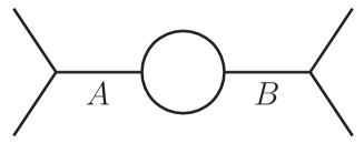
Figure 2: Internal lines that, if broken, disconnect the diagram

Formula (2.5) applies to any line that, if broken, disconnects the diagram. Examples are the lines A or B in fig. 2. It cannot be used inside the loop diagrams, as shown in ref. [24] (see also [6]), but this is not of our concern in the present paper.

If $(-i)\Sigma(p^{2})$ denotes the amputated 1PI $\chi$ two-point function, the formal resummation gives the dressed propagator

$$\hat{P}_{\chi}=P_{\chi}\sum_{n=0}^{\infty}(-i\Sigma P_{\chi})^{n}=\frac{i(p^{2}-m^{2})}{(p^{2}-m^{2})[p^{2}-m^{2}-\Sigma(p^{2})]+\epsilon^{2}}.$$ (2.6)

When we do not specify the arguments of $P_{\chi}$, we mean $P_{\chi}(p^{2},m^{2},\epsilon)$.

If we study the approximation (2.3) around the peak, we find that $\Gamma$ is nonnegative again, by the optical theorem. It receives contributions from the physical particles circulating in the 1PI $\chi$ two-point function. The formal result is thus

$$\hat{P}_{\chi}\simeq\frac{iZ(p^{2}-m^{2})}{(p^{2}-m^{2})(p^{2}-m_{\text{ph}}^{2}+im_{\text{ph}}\Gamma)+\tilde{\epsilon}^{2}}.$$ (2.7)

where $\tilde{\epsilon}=\epsilon Z^{1/2}$.

There are actually other options to perform the resummation in the case of purely virtual particles. Since we cannot predict the final outcome in the peak region, which, as we have anticipated, triggers nonperturbative effects, it is interesting to explore the alternatives. In particular, the powers of $\Delta m^{2}$ redefine the squared mass, which may or may not have an impact on the problems we consider here. Formula (2.7) describes the situation where they do. If we assume that they do not, we can proceed as explained in appendix A, where we resum $\Delta m^{2}$ by default into $m_{\text{ph}}^{2}$. The result is

$$\hat{P}_{\chi}\simeq\frac{iZ(p^{2}-m_{\text{ph}}^{2})}{(p^{2}-m_{\text{ph}}^{2})(p^{2}-m_{\text{ph}}^{2}+im_{\text{ph}}\Gamma)+\tilde{\epsilon}^{2}}.$$ (2.8)

Summarizing, we have two candidates for the dressed propagator of purely virtual particles: (2.7) and (2.8). Neither is satisfactory, though. We can see it by noting that, in the limit $\tilde{\epsilon}\rightarrow 0$, both (2.7) and (2.8) give the same result we obtain from the physical particle, formula (2.4). The difference between a fakeon and a physical particle appears to be washed away by the resummation. This cannot be correct, since if we expand the sums we must find back what we summed.

Something suspicious is the simplification of $p^{2}-m^{2}$ in (2.7) and $p^{2}-m_{\text{ph}}^{2}$ (2.8) between the numerator and the denominator when $\tilde{\epsilon}$ tends to zero. The point is that we cannot take the limit $\tilde{\epsilon}\rightarrow 0$ so naively.

2.3 Ghosts

Ghosts $\phi$ have the tree-level propagator

$$P_{\phi}(p^{2},m^{2},\epsilon)=-\frac{i}{p^{2}-m^{2}+i\epsilon}.$$ (2.9)

Although the prescription is the Feynman one, the minus sign in front makes a crucial difference, as we are going to show. If, as before, $(-i)\Sigma(p^{2})$ denotes the amputated 1PI $\phi$ two-point function, the resummation gives

$$\hat{P}_{\phi}=P_{\phi}\sum_{n=0}^{\infty}(-i\Sigma P_{\phi})^{n}=-\frac{i}{p^{2}-m^{2}+\Sigma(p^{2})+i\epsilon}.$$

For convenience, we rearrange the approximation (2.3) around $p^{2}\simeq m^{2}$ as

$$\Sigma(p^{2})\simeq Z^{-1}(-\Delta m^{2}-im_{\text{ph}}\Gamma)+(Z^{-1}-1)(p^{2}-m^{2}),\qquad m_{\text{ph}}^{2}\equiv m^{2}+\Delta m^{2},\qquad\Gamma\geqslant 0,$$ (2.10)

by changing the conventions for $\Delta m^{2}$ and $Z$. We can still assume $\Gamma\geqslant 0$, because, if $\phi$ “decays” into lighter physical particles, $-i\Sigma$ is the same as before at one loop around $p^{2}\simeq m^{2}$. We obtain

$$\hat{P}_{\phi}\simeq-\frac{iZ}{p^{2}-m_{\text{ph}}^{2}+i(\tilde{\epsilon}-m_{\text{ph}}\Gamma)}$$ (2.11)

close to the ghost peak, where $\tilde{\epsilon}=\epsilon Z$. Note the crucial sign difference appearing in $\tilde{\epsilon}-m_{\text{ph}}\Gamma$ with respect to (2.4). Again, we cannot take the limit $\tilde{\epsilon}\rightarrow 0$ naively, because it reverses the prescription.

3 Differences among physical particles, fake particles and ghosts

In this section we analyze of the differences among the perturbative expansions of $\hat{P}_{\varphi}$, $\hat{P}_{\chi}$ and $\hat{P}_{\phi}$. We assume $Z=1$ and $\Delta m^{2}=0$, to simplify the formulas and concentrate on the effects of the width $\Gamma$. We also assume that $m$ and $\Gamma$ are the same in the three cases. We have

$$\hat{P}_{\varphi} \simeq \frac{i}{p^{2}-m^{2}+i(\epsilon+m\Gamma)},\qquad\hat{P}_{\chi}\simeq\frac{i(p^{2}-m^{2})}{(p^{2}-m^{2})(p^{2}-m^{2}+im\Gamma)+\epsilon^{2}},$$

$$\hat{P}_{\phi} \simeq -\frac{i}{p^{2}-m^{2}+i(\epsilon-m\Gamma)},$$ (3.1)

respectively.

Since $\epsilon$ is a mathematical artifact, it must tend to zero at the end. We can take two attitudes towards this limit: we can study the limit $\epsilon\rightarrow 0$ term by term in the perturbative expansion and then resum; or first resum and let $\epsilon\rightarrow 0$ at the end. The former is what perturbative quantum field theory asks us to do, strictly speaking, so for the time being we concentrate on this option.

The formulas (3.1) have to be meant as shorthand expressions for their perturbative expansions, which are the expansion in powers of $\Gamma$. We show that, in the cases of purely virtual particles and ghosts, the resummations are not legitimate, because they do not make sense as mathematical distributions. We mostly concentrate on the real parts, but the arguments and results easily extend to the whole $\hat{P}_{\varphi}$, $\hat{P}_{\chi}$ and $\hat{P}_{\phi}$.

3.1 Difference with ghosts

It is convenient to start from the difference Im$[im^{2}(\hat{P}_{\varphi}-\hat{P}_{\phi})]$ between physical particles and ghosts, which can be written as

$$\text{Im}[im^{2}(\hat{P}_{\varphi}-\hat{P}_{\phi})]=\frac{i}{2}\left[\frac{1}{x+i\hat{\Gamma}+i\hat{\epsilon}}-\frac{1}{x+i\hat{\Gamma}-i\hat{\epsilon}}+\frac{1}{x-i\hat{\Gamma}+i\hat{\epsilon}}-\frac{1}{x-i\hat{\Gamma}-i\hat{\epsilon}}\right],$$ (3.2)

where $x\equiv(p^{2}-m^{2})/m^{2}$, $\hat{\epsilon}=\epsilon/m^{2}$ and $\hat{\Gamma}=\Gamma/m$. Naively, the right-hand side tends to zero when $\hat{\epsilon}$ tends to zero. Considering $\pm i\hat{\Gamma}$ as shifts of $x$, and recalling that we are working on the series expansions in powers of $\hat{\Gamma}$, we can formally write

$$\left.\text{Im}[im^{2}(\hat{P}_{\varphi}-\hat{P}_{\phi})]\right|_{\hat{\epsilon}\rightarrow 0}=\pi\left[\delta(x+i\hat{\Gamma})+\delta(x-i\hat{\Gamma})\right]=2\pi\sum_{n=0}^{\infty}\frac{(-\hat{\Gamma}^{2})^{n}}{(2n)!}\delta^{(2n)}(x).$$ (3.3)

The expressions $\delta(x\pm i\hat{\Gamma})$ are, again, shorthand notations for their perturbative expansions in powers of $\hat{\Gamma}$. We see that the difference (3.2) is not zero, but an infinite series of contact terms. Now, Im$[im^{2}\hat{P}_{\varphi}]$ resums into a well-behaved function, which is the Breit-Wigner formula

$$\text{Im}[im^{2}\hat{P}_{\varphi}]=\frac{\hat{\epsilon}+\hat{\Gamma}}{x^{2}+(\hat{\epsilon}+\hat{\Gamma})^{2}}\underset{\hat{\epsilon}\rightarrow 0}{\longrightarrow}\frac{\hat{\Gamma}}{x^{2}+\hat{\Gamma}^{2}}.$$

We conclude that $\left.\text{Im}[im^{2}\hat{P}_{\phi}]\right|_{\hat{\epsilon}\rightarrow 0}$ is equal to the same thing minus $2\pi\Delta_{\hat{\Gamma}}(x)$, where

$$\Delta_{\hat{\Gamma}}(x)\equiv\sum_{n=0}^{\infty}\frac{(-\hat{\Gamma}^{2})^{n}}{(2n)!}\delta^{(2n)}(x)=\frac{1}{2}[\delta(x+i\hat{\Gamma})+\delta(x-i\hat{\Gamma})].$$ (3.4)

The question is: what is $\Delta_{\hat{\Gamma}}(x)$? Evidently, it is not a function. We could accept it as a mathematical distribution. In appendix B we show in detail that it is not even a distribution. Here we discuss the physical meaning of this fact.

At the practical level, we cannot determine the momenta of the incoming particles with absolute precision, so the true incoming state can be written as a superposition

$$|\text{in}\rangle=\int\frac{\mathrm{d}^{3}\mathbf{k}_{1}}{2k_{1}^{0}(2\pi)^{3}}\frac{\mathrm{d}^{3}\mathbf{k}_{2}}{2k_{2}^{0}(2\pi)^{3}}f_{1}(\mathbf{k}_{1})f_{2}(\mathbf{k}_{2})|\mathbf{k}_{1},\mathbf{k}_{2},\text{in}\rangle,$$

where $f_{1}(\mathbf{k}_{1})$ and $f_{2}(\mathbf{k}_{2})$ are the amplitudes of the wave packets and $|\mathbf{k}_{1},\mathbf{k}_{2},$in$\rangle$ denotes the ideal state where the incoming particles have definite momenta $\mathbf{k}_{1}$ and $\mathbf{k}_{2}$. Mathematically, the wave packets can be seen as test functions and the correlation functions as distributions.

If we choose the wave packets in a suitable way, $\Delta_{\hat{\Gamma}}(x)$ originates absurdities of new types (not directly related the violations of unitarity, typical of ghosts). For example, if we take the convolution of the function $\Delta_{\hat{\Gamma}}(x)$ with certain wave packets of incoming momenta, we can generate a pole at $p^{2}=m^{2}$ out of nowhere, with no width:

$$\int_{-\infty}^{+\infty}\mathrm{d}y\hskip 0.72229pt\Delta_{\hat{\Gamma}}(x-y)\frac{y}{y^{2}+\hat{\Gamma}^{2}}=\frac{1}{x}\frac{x^{2}+2\hat{\Gamma}^{2}}{x^{2}+4\hat{\Gamma}^{2}}=\frac{m^{2}}{p^{2}-m^{2}}\frac{(p^{2}-m^{2})^{2}+2m^{2}\Gamma^{2}}{(p^{2}-m^{2})^{2}+4m^{2}\Gamma^{2}}.$$

3.2 Perturbative expansions by means of distributions

To extend this analysis to purely virtual particles and study $\hat{P}_{\varphi}$, $\hat{P}_{\chi}$ and $\hat{P}_{\phi}$ further, it is useful to work out a systematic expansion by means of distributions. For example, if we use identities such as

$$\frac{\mathrm{d}}{\mathrm{d}\hat{\epsilon}}\frac{\hat{\epsilon}}{x^{2}+\hat{\epsilon}^{2}}=-\frac{\mathrm{d}}{\mathrm{d}x}\frac{x}{x^{2}+\hat{\epsilon}^{2}},\qquad\frac{\mathrm{d}}{\mathrm{d}\hat{\epsilon}}\frac{x}{x^{2}+\hat{\epsilon}^{2}}=\frac{\mathrm{d}}{\mathrm{d}x}\frac{\hat{\epsilon}}{x^{2}+\hat{\epsilon}^{2}},$$

the expansion of the Breit-Wigner formula is immediately obtained:

$$\text{Im}[im^{2}\hat{P}_{\varphi}]=\frac{\hat{\epsilon}+\hat{\Gamma}}{x^{2}+(\hat{\epsilon}+\hat{\Gamma})^{2}}=\sum_{n=0}^{\infty}\frac{\hat{\Gamma}^{n}}{n!}\frac{\mathrm{d}^{n}}{\mathrm{d}\hat{\epsilon}^{n}}\frac{\hat{\epsilon}}{x^{2}+\hat{\epsilon}^{2}}\rightarrow\pi\Delta_{\hat{\Gamma}}(x)+\frac{1}{\hat{\Gamma}}\sum_{n=0}^{\infty}\frac{(-\hat{\Gamma}^{2})^{n+1}}{(2n+1)!}\mathcal{P}^{(2n+1)}\frac{1}{x},$$ (3.5)

where $\mathcal{P}^{(k)}$ denotes the $k$-th derivative of the Cauchy principal value. We have taken $\hat{\epsilon}$ to zero term by term in the last expression.

In the case of ghosts, the same procedure gives

$$\text{Im}[im^{2}\hat{P}_{\phi}]=\frac{\hat{\Gamma}-\hat{\epsilon}}{x^{2}+(\hat{\Gamma}-\hat{\epsilon})^{2}}\rightarrow-\pi\Delta_{\hat{\Gamma}}(x)+\frac{1}{\hat{\Gamma}}\sum_{n=0}^{\infty}\frac{(-\hat{\Gamma}^{2})^{n+1}}{(2n+1)!}\mathcal{P}^{(2n+1)}\frac{1}{x}.$$ (3.6)

The derivatives of the principal values disappear in the difference Im$[im^{2}(\hat{P}_{\varphi}-\hat{P}_{\phi})]$, which confirms (3.3). Thus, the powers of $\Gamma$ cannot be resummed at $\hat{\epsilon}=0$ in the case of ghosts.

3.3 Difference with purely virtual particles

Now we switch to fakeons. If we want to resum the powers of $\Gamma$ at $\hat{\epsilon}=0$, we must deal with

$$\text{Im}[im^{2}\hat{P}_{\chi}]=\frac{x^{2}\hat{\Gamma}}{(x^{2}+\hat{\epsilon}^{2})^{2}+x^{2}\hat{\Gamma}^{2}}=-\frac{1}{\hat{\Gamma}}\sum_{n=0}^{\infty}\frac{(-x^{2}\hat{\Gamma}^{2})^{n+1}}{(x^{2}+\hat{\epsilon}^{2})^{2n+2}}.$$

Taking $\hat{\epsilon}\rightarrow 0$ term by term in the last expression, we obtain powers of the Cauchy principal value, which can be treated by means of the coincidence-splitting method explained in appendix C, formula (C.1), Thus,

$$\text{Im}[im^{2}\hat{P}_{\chi}]\rightarrow\frac{1}{\hat{\Gamma}}\sum_{n=0}^{\infty}\frac{(-\hat{\Gamma}^{2})^{n+1}}{(2n+1)!}\mathcal{P}^{(2n+1)}\frac{1}{x}.$$ (3.7)

The difference with respect to the physical particle is one half of (3.3):

$$\text{Im}[im^{2}(\hat{P}_{\varphi}-\hat{P}_{\chi})]\rightarrow\pi\Delta_{\hat{\Gamma}}(x).$$

It is clear that only the physical combination (3.5) is well defined, while (3.6) and (3.7) are not, since $\Delta_{\hat{\Gamma}}(x)$ is not a distribution. The real parts of $im^{2}\hat{P}_{\varphi,\chi,\phi}$ can be studied similarly and lead to analogous conclusions.

The perturbative expansion is missing something. On the one hand, the differences proportional to $\Delta_{\hat{\Gamma}}(x)$ cannot be ignored. On the other hand, they do not describe what is missing accurately enough, due to the (mathematical and physical) difficulties of $\Delta_{\hat{\Gamma}}(x)$. As we are going to show in the next sections, the problems become nonperturbative around the peaks of purely virtual particles and ghosts.

4 Dressed propagator of physical particles

In this section we discuss the convergence of the formal resummation (2.4) in the case of physical particles $\varphi$, pointing out several nontrivial facts, to prepare the discussion of the next section about purely virtual particles. We assume that $\Gamma$, $\Delta m^{2}$ and $Z-1$ are generic, of order $\lambda^{2}$ in some (small) dimensionless coupling $\lambda$.

The condition of convergence for the resummation (2.2) is (keeping $\epsilon$ for future use)

$$\frac{|\Sigma(p^{2})|}{|p^{2}-m^{2}+i\epsilon|}<1.$$ (4.1)

It can be refined by combining it with the approximation (2.3) and using (2.4). For example, $Z$ just affects the overall constant, so the corrections due to it can be resummed first with no difficulties. Once the powers of $Z-1$ are resummed, we can focus on the resummation of the powers of $\Gamma$ and $\Delta m^{2}$, which is convergent for

$$\frac{(\Delta m^{2})^{2}+m_{\text{ph}}^{2}\Gamma^{2}}{(p^{2}-m^{2})^{2}+\tilde{\epsilon}^{2}}<1,$$ (4.2)

i.e., sufficiently away from the peak region, which is $p^{2}\simeq m_{\text{ph}}^{2}=m^{2}+\Delta m^{2}$. If we resum the powers of $\Delta m^{2}$ into $m_{\text{ph}}^{2}$ by default, and focus on the powers of $\Gamma$, then the convergence condition reads

$$\frac{m_{\text{ph}}^{2}\Gamma^{2}}{(p^{2}-m_{\text{ph}}^{2})^{2}+\tilde{\epsilon}^{2}}<1.$$ (4.3)

The validity of the resummation can be extended beyond the bounds just found, thanks to analyticity.

A priori, we cannot be sure that analyticity holds after the resummation, so we treat it as a work hypothesis. A second hypothesis is that essential singularities, which are invisible at the level of the perturbative expansion, do not contribute or are negligible. These assumptions can be validated or rejected by experiments.

The correct why to phrase what is happening is as follows. Since

a) the Feynman prescription is analytic and

b) the denominator of (2.4) never vanishes,

there is an analytic way to extend the result beyond the region of convergence, that is to say, close to the peak. Moreover, since

c) experiments support the result obtained this way,

the resummed $\hat{P}_{\varphi}$ is correct and the resummation holds everywhere.

4.1 The problem of the muon and its solution

The comparison between experiments and theoretical predictions requires further analysis. Let us consider a process like $e^{+}e^{-}\rightarrow e^{+}e^{-}$. The contribution $\mathcal{M}_{\varphi}$ of the diagrams of fig. 1 to the total amplitude $\mathcal{M}$ of the process is equal to $i\hat{P}_{\varphi}$ (assuming that the external vertices are equal to $-i$). Typically, $\mathcal{M}_{\varphi}$ is the dominant contribution in a neighborhood of $p^{2}=m_{\text{ph}}^{2}$. In what follows, we concentrate on it.

By the optical theorem, the imaginary part Im$[2\mathcal{M}]$ is proportional to the sum of the cross sections of the processes $e^{+}e^{-}\rightarrow$ $X$, where $X$ denotes any set of outgoing states. The processes involved in 2Im$[\mathcal{M}_{\varphi}]$, which can be read by cutting the diagrams as shown in fig. 3, are

$$e^{+}e^{-}\rightarrow\varphi,\qquad e^{+}e^{-}\rightarrow\text{decay products of }\varphi\text{.}$$

The former is the process where the particle is physically observed before it decays (as in the case $\varphi$ = muon). The latter is the process where $\varphi$ is not observed directly (typically, because its lifetime is too short, as in the case $\varphi$ = $Z$ boson): its decay products are observed, instead. Thus, we have

$$2\text{Im}[\mathcal{M}_{\varphi}]\simeq\int\mathrm{d}\Pi_{f}\hskip 0.72229pt|\mathcal{M}_{e^{+}e^{-}\rightarrow\varphi}|^{2}+\int\mathrm{d}\Pi_{f}\hskip 0.72229pt|\mathcal{M}_{e^{+}e^{-}\rightarrow\text{decay products of }\varphi}|^{2},$$ (4.4)

around the $\varphi$ peak.

Diagrammatically, the two contributions correspond to the first and second lines of fig. 3, which give the sums reported in formulas (C.3) of appendix C. The integrals on the phase spaces $\Pi_{f}$ of the outgoing states are originated by the cut propagators, according to the rules of cut diagrams. The vertices and propagators that lie to the right of the cut are the normal ones (as in $\mathcal{M}$), while those that lie to the left of the cut are the complex conjugate ones (as in $\mathcal{M}^{\dagger}$). We are assuming that the energy flows from the right to the left.

We have, from (2.2) and (C.3),

$$2\text{Im}[\mathcal{M}_{\varphi}]=2\text{Re}[\hat{P}_{\varphi}]=\frac{2(\epsilon-\text{Im}[\Sigma])}{|p^{2}-m^{2}-\Sigma+i\epsilon|^{2}}=2\Omega_{\varphi\hskip 0.72229pt\text{particle}}+2\Omega_{\varphi\hskip 0.72229pt\text{decay}},$$

where

$$2\Omega_{\varphi\hskip 0.72229pt\text{particle}} = \frac{2\epsilon}{|p^{2}-m^{2}-\Sigma+i\epsilon|^{2}}\underset{\epsilon\rightarrow 0}{\longrightarrow}\int\mathrm{d}\Pi_{f}\hskip 0.72229pt|\mathcal{M}_{e^{+}e^{-}\rightarrow\varphi}|^{2},$$ (4.5)

$$2\Omega_{\varphi\hskip 0.72229pt\text{decay}} = -\frac{2\text{Im}[\Sigma]}{|p^{2}-m^{2}-\Sigma+i\epsilon|^{2}}\underset{\epsilon\rightarrow 0}{\longrightarrow}\int\mathrm{d}\Pi_{f}\hskip 0.72229pt|\mathcal{M}_{e^{+}e^{-}\rightarrow\text{decay products of }\varphi}|^{2}.$$ (4.6)

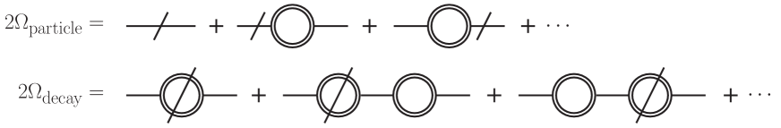
Figure 3: Cut diagrams contributing to $2\Omega_{\text{particle}}$ and $2\Omega_{\text{decay}}$, respectively

Using the approximation (2.3) around the peak, we find

$$\Omega_{\varphi\hskip 0.72229pt\text{particle}} \simeq \frac{\tilde{\epsilon}Z}{(p^{2}-m_{\text{ph}}^{2})^{2}+(\tilde{\epsilon}+m_{\text{ph}}\Gamma)^{2}},$$ (4.7)

$$\Omega_{\varphi\hskip 0.72229pt\text{decay}} \simeq \frac{m_{\text{ph}}Z\Gamma}{(p^{2}-m_{\text{ph}}^{2})^{2}+(\tilde{\epsilon}+m_{\text{ph}}\Gamma)^{2}}.$$ (4.8)

Again, we can let $\epsilon$ tend to zero before or after the resummation. Here we study the limit $\epsilon\rightarrow 0$ after the resummation, below (and in appendix C) we say more about the limit before the resummation.

Taking $\epsilon$ to zero in (4.7) and (4.8), we obtain

$$\Omega_{\varphi\hskip 0.72229pt\text{particle}}\rightarrow 0,\qquad\Omega_{\varphi\hskip 0.72229pt\text{decay}}\rightarrow\frac{m_{\text{ph}}Z\Gamma}{(p^{2}-m_{\text{ph}}^{2})^{2}+m_{\text{ph}}^{2}\Gamma^{2}}.$$ (4.9)

The conclusion is that an unstable particle has zero probability of being observed. Such a result is in contradiction with experiments, since the muon is unstable, but can be observed before it decays: $\Omega_{\varphi\hskip 0.72229pt\text{particle}}$ should not be zero; $\Omega_{\varphi\hskip 0.72229pt\text{decay}}$ should vanish, instead. This is what we call “the problem of the muon”.

In quantum field theory a number of shortcuts are commonly adopted to simplify the derivations of general formulas. In particular, the scattering processes are usually meant to occur between incoming states at $t=-\infty$ and outgoing states at $t=+\infty$. Since the time interval $\Delta t$ separating them is, strictly speaking, infinite, every unstable particle has enough time to decay before being observed, in agreement with the result $\Omega_{\varphi\hskip 0.72229pt\text{particle}}=0$ obtained above. In this sense, there is no contradiction. However, the observation of the muon is a fact and we should be able to account for it.

In practical situations the scattering processes occur within some finite time interval $\Delta t$, much larger than the duration $\bar{\Delta}t$ of the interactions involved in the process. The prediction $\Omega_{\varphi\hskip 0.72229pt\text{particle}}=0$ remains correct whenever $\Delta t$ is also much larger than, say, the muon lifetime $\tau_{\mu}$. We have a problem for $\bar{\Delta}t\ll\Delta t<\tau_{\mu}$, since the muon has not enough time to decay in that case. After the resummation of the self-energies into the dressed propagator, we still obtain the prediction $\Omega_{\varphi\hskip 0.72229pt\text{particle}}=0$, which is in contradiction with the phenomenon we observe.

In principle, we should undertake the task of rederiving all the basic formulas of quantum field theory for scattering processes where incoming and outgoing states are separated by a finite $\Delta t$. Once we do so, the predictions end up depending on $\Delta t$. They also depend on the energy resolution $\Delta E\sim 1/\bar{\Delta}t$, where $\bar{\Delta}t$ is the time uncertainty. Indeed, only $\Delta t=\infty$ is compatible with infinite energy resolution (since $\bar{\Delta}t\leqslant\Delta t$, $\Delta E=0$ implies $\Delta t=\infty$). However, the energy resolution has to do with the experimental setup, so there might be no universal way to include it. One may have to use different formulas, depending on the experiment.

Instead of going through this, we can try and guess how $\Delta E$ may affect the results. Generically, $\Delta E$ can appear more or less everywhere, but in most places it redefines quantities that are already present, so we can neglect it. The $\Delta E$ dependence cannot be ignored if it affects the imaginary part of the denominator of the propagator, which survives the free-field limit. An effect of this type is not surprising, if we consider that $\Delta E$ is associated with the time resolution $\bar{\Delta}t$, which must be compared with the particle lifetime, which in turn is the reciprocal of the width.

The energy resolution we focus on is the one around the peak. Specifically, we define the “distance” in energy from the peak as the ratio

$$\frac{|p^{2}-m_{\text{ph}}^{2}|}{2m_{\text{ph}}}.$$ (4.10)

Then the (Lorentz invariant) meaning of $\Delta E$ is that we cannot resolve momenta $p$ that are closer than $\Delta E$ to the peak.

In light of the remarks just made, we assume that when $\Delta E$ is different from zero the predictions coincide with the ones we have written above once we make the replacement

$$\tilde{\epsilon}\rightarrow\tilde{\epsilon}+2m_{\text{ph}}\Delta E,$$ (4.11)

after which we can take $\tilde{\epsilon}$ to zero, since at that point it is no longer necessary.

The form of the $\Delta E$ dependence in (4.11) is not crucial, as long as the correction vanishes when $\Delta E$ tends to zero. For example, variants such as

$$\tilde{\epsilon}\rightarrow\tilde{\epsilon}+\gamma m_{\text{ph}}\Delta E\left(\frac{\Delta E}{m_{\text{ph}}}\right)^{\delta},$$ (4.12)

with $\gamma>0$, $\delta>-1$, do not change the conclusions we derive. Indeed, (4.11) vs (4.12) is just a redefinition of $\Delta E$ into a function of $\Delta E$, which only affects the relations between $\Delta t$, $\bar{\Delta}t$ and $\Delta E$.

Making the replacement in formulas (4.7) and (4.8) and letting $\tilde{\epsilon}$ tend to zero, we obtain

$$\Omega_{\varphi\hskip 0.72229pt\text{particle}} \simeq \frac{2m_{\text{ph}}Z\Delta E}{(p^{2}-m_{\text{ph}}^{2})^{2}+m_{\text{ph}}^{2}(2\Delta E+\Gamma)^{2}},$$ (4.13)

$$\Omega_{\varphi\hskip 0.72229pt\text{decay}} \simeq \frac{m_{\text{ph}}Z\Gamma}{(p^{2}-m_{\text{ph}}^{2})^{2}+m_{\text{ph}}^{2}(2\Delta E+\Gamma)^{2}},$$ (4.14)

The results show that $\Omega_{\varphi\hskip 0.72229pt\text{particle}}$ is no longer zero.

From the phenomenological side, we may distinguish three cases:

— Case of the $Z$ boson. Here $\Delta E\ll\Gamma/2$, so

$$\Omega_{\varphi\hskip 0.72229pt\text{particle}}\simeq 0,\qquad\Omega_{\varphi\hskip 0.72229pt\text{decay}}\simeq\frac{m_{\text{ph}}Z\Gamma}{(p^{2}-m_{\text{ph}}^{2})^{2}+m_{\text{ph}}^{2}\Gamma^{2}}.$$

In agreement with experiment, the predictions tell us that we do not see the particle: we see its decay products. The results do not depend on $\Delta E$ to the first degree of approximation.

— Case of the muon. Here $m_{\text{ph}}\gg\Delta E\gg\Gamma/2$, so

$$\Omega_{\varphi\hskip 0.72229pt\text{particle}}\simeq\frac{2m_{\text{ph}}Z\Delta E}{(p^{2}-m_{\text{ph}}^{2})^{2}+4m_{\text{ph}}^{2}\Delta E^{2}}\simeq\pi Z\delta(p^{2}-m_{\text{ph}}^{2}),\qquad\Omega_{\varphi\hskip 0.72229pt\text{decay}}\simeq 0.$$ (4.15)

These results do not depend on $\Delta E$ to the first degree of approximation and tell us that we see the particle, not its decay products, in agreement with experiment.

— Intermediate situations. When $\Delta E$ and $\Gamma$ are comparable, we see both the particle and its decay products. The results depend on $\Delta E$ and so does the ratio $\Omega_{\varphi\hskip 0.72229pt\text{particle}}/\Omega_{\varphi\hskip 0.72229pt\text{decay}}=2\Delta E/\Gamma.$

We have uncovered, among the other things, that it is impossible to explain the observation of the muon, i.e., derive $\Omega_{\varphi\hskip 0.72229pt\text{particle}}\simeq\pi Z\delta(p^{2}-m_{\text{ph}}^{2})$ in (4.15), without introducing the resolution $\Delta E$, even if the final result is independent of $\Delta E$ (because the approximations valid for the muon make it disappear). This fact can be understood as a consequence of the energy-time uncertainty relation $\Delta E\hskip 0.72229pt\sim 1/\bar{\Delta}t$. Indeed, $\Delta E=0$ implies an infinite time uncertainty, during which every unstable particle has enough time to decay before being observed: it is impossible to observe an unstable particle with infinite resolving power on its energy.

This impossibility can also be appreciated by studying the limit $\epsilon\rightarrow 0$ term by term, before the resummation. In subsection 4.3 and in appendix C, we show that each term of the expansions of $\Omega_{\varphi\hskip 0.72229pt\text{particle}}$ and $\Omega_{\varphi\hskip 0.72229pt\text{decay}}$ is ill defined at $\Delta E=0$, apart from a few ones: only the expansion of the sum $\Omega_{\varphi\hskip 0.72229pt\text{particle}}+\Omega_{\varphi\hskip 0.72229pt\text{decay}}$ is regular. Such a complication, which may sound surprising at first, is actually unavoidable, precisely because a regular $\Omega_{\varphi\hskip 0.72229pt\text{particle}}$ at $\Delta E=0$ would violate the energy-time uncertainty relation, in the case of unstable particles. Quantum field theory knows it, so to speak, and retaliates by creating problems in the crucial places. These properties emphasize that the issues we are discussing here concern not only new or unusual quantization prescriptions, but also physical particles, although in different ways.

Another important observation is that the replacement (4.11) violates unitarity at nonvanishing $\Delta E$. Indeed, a propagator (2.1) with $\epsilon\rightarrow\epsilon+2m_{\text{ph}}Z^{-1}\Delta E$ comes from a non-Hermitian Lagrangian. When the experimental setup has an important impact on the predictions, we cannot consider the system as an isolated one, so unitarity as we normally understand it may not hold. Nevertheless, as long as $\Delta E$ tends to zero after the expansion in powers of $\Gamma$, the replacement (4.11) is precisely the right one to have perturbative unitarity, because $\Delta E$ plays the role of the infinitesimal width $\epsilon$.

4.2 Conditions of convergence

Let us discuss the convergence radius after the replacement (4.11). Since $\Delta E$ is independent of the interactions (it affects the propagator already at the tree level), the condition (4.2) for convergence is

$$\frac{(\Delta m^{2})^{2}+m_{\text{ph}}^{2}\Gamma^{2}}{(p^{2}-m^{2})^{2}+4m_{\text{ph}}^{2}\Delta E^{2}}<1.$$ (4.16)

It is possible to satisfy this condition for every $p$ if and only if

$$\Delta E>\frac{1}{2m_{\text{ph}}}\sqrt{m_{\text{ph}}^{2}\Gamma^{2}+(\Delta m^{2})^{2}}\equiv\Delta E_{\text{min}}.$$ (4.17)

If we assume that the powers of $\Delta m^{2}$ are resummed by default into the physical mass $m_{\text{ph}}$, we can use (4.11) inside (4.3), so the convergence condition becomes

$$\frac{m_{\text{ph}}^{2}\Gamma^{2}}{(p^{2}-m_{\text{ph}}^{2})^{2}+4m_{\text{ph}}^{2}\Delta E^{2}}<1,$$ (4.18)

which holds for every $p$ if and only if

$$\Delta E>\frac{\Gamma}{2}\equiv\Delta E_{\text{min}}.$$ (4.19)

The validity of the resummation can be extended to the peak region, i.e., beyond the bounds (4.17) or (4.19), by means of analyticity. Yet, it is crucial for the discussion that follows to remember that there is a region where the convergence is guaranteed and a region that can only be reached by means of analyticity. When analyticity does not hold, the peak region cannot be reached.

Note that the left-hand sides of (4.16) and (4.18) are the expansion parameters. When the inequalities (4.16) or (4.18) do not hold, the problem is nonperturbative, not because the coupling is large, but because the expansion parameter is large, due to its $p$ dependence. Specifically, if $\Delta E$ vanishes or is too small, (4.16) and (4.18) are violated in the peak region $|p^{2}-\tilde{m}^{2}|\leqslant 2m_{\text{ph}}\Delta E_{\text{min}}$ no matter how small the coupling is, where $\tilde{m}$ is $m$ or $m_{\text{ph}}$ depending on the case.

4.3 Ill-defined sums with physical particles

Now we show that ill-defined distributions also concern physical (unstable) particles, when their observation is considered separately from the observation of their decay products. To achieve this goal, we study the limit $\epsilon\rightarrow 0$ term by term in the expansions of $\Omega_{\varphi\hskip 0.72229pt\text{particle}}$ and $\Omega_{\varphi\hskip 0.72229pt\text{decay}}$, before their resummations.

The perturbative expansion of $\Omega_{\varphi\hskip 0.72229pt\text{particle}}$ reads, from formula (4.5),

$$\frac{\epsilon}{|p^{2}-m^{2}-\Sigma+i\epsilon|^{2}}=\frac{\epsilon}{(p^{2}-m^{2})^{2}+\epsilon^{2}}+2\frac{\epsilon(p^{2}-m^{2})\text{Re}[\Sigma]+\epsilon^{2}\text{Im}[\Sigma]}{((p^{2}-m^{2})^{2}+\epsilon^{2})^{2}}+\mathcal{O(}\Sigma^{2}).$$

The zeroth order is $\pi\delta(p^{2}-m^{2})$, while the $\mathcal{O(}\Sigma)$ term proportional to Re$[\Sigma]$ gives $\delta^{\prime}(p^{2}-m^{2})$. It is easy to check that the $\mathcal{O(}\Sigma)$ term proportional to Im$[\Sigma]$ is not a distribution. Something similar happens at higher orders. Using the approximation (2.3) and concentrating on the expansion in powers of $\Gamma$, we obtain, from (4.7),

$$\Omega_{\varphi\hskip 0.72229pt\text{particle}}\simeq\pi Z\delta(p^{2}-m_{\text{ph}}^{2})-\frac{2\tilde{\epsilon}^{2}m_{\text{ph}}Z\Gamma}{((p^{2}-m_{\text{ph}}^{2})^{2}+\tilde{\epsilon}^{2})^{2}}+\mathcal{O}(\Gamma^{2}).$$ (4.20)

The practical consequence is that, when we make the replacement (4.11) and set $\epsilon=0$, we get corrections that are very large for $\Delta E\ll\Gamma/2$. The ill-defined distributions (or large contributions) just described mutually cancel in the sums (4.13) plus (4.14), (4.7) plus (4.8) and (4.5) plus (4.6).

The technical problems arise because we are trying to separate the observation of the particle from the observation of its decay products. Since a propagator is the sum of a Cauchy principal value and a Dirac delta function, arbitrary powers of such distributions are generated. A way to define them is by means of the symmetric coincidence-splitting method described in appendix C. Working out the two lines of fig. 3 with this method, we obtain formulas (C.4) for $\Omega_{\varphi\hskip 0.72229pt\text{particle}}$ and $\Omega_{\varphi\hskip 0.72229pt\text{decay}}$. The sum $\Omega_{\varphi\hskip 0.72229pt\text{particle}}+\Omega_{\varphi\hskip 0.72229pt\text{decay}}$ is well defined and coincides with what we expect, as shown in equation (C.5), but $\Omega_{\varphi\hskip 0.72229pt\text{particle}}$ and $\Omega_{\varphi\hskip 0.72229pt\text{decay}}$, taken separately, are ill-defined distributions, similar to $\Delta_{\hat{\Gamma}}$.

Finally, formula (4.14) gives

$$\Omega_{\varphi\hskip 0.72229pt\text{decay}}\simeq\frac{\Gamma}{2\Delta E}\frac{2m_{\text{ph}}Z\Delta E}{(p^{2}-m_{\text{ph}}^{2})^{2}+4m_{\text{ph}}^{2}\Delta E^{2}}$$

for $\Gamma\ll 2\Delta E$, which shows that we cannot observe the “peak of the muon”. Instead, we observe a much smaller bump entirely due to the nonvanishing energy resolution of our experimental setup.

5 Dressed propagator of purely virtual particles

In this section we investigate the resummation of the self-energies in the case of purely virtual particles $\chi$. The contribution to the amplitude is $\mathcal{M}_{\chi}=i\hat{P}_{\chi}$ and $\text{Im}[\mathcal{M}_{\chi}]=\text{Re}[\hat{P}_{\chi}]\simeq\Omega_{\chi\hskip 0.72229pt\text{\textquotedblleft decay\textquotedblright}}$: there is no $\Omega_{\chi\hskip 0.72229pt\text{\textquotedblleft particle\textquotedblright}}$ in the case of fakeons. Indeed, the diagrams shown in the first line of fig. 3 vanish identically, because a fakeon does not appear among the final states (its cut propagator being zero). For the same reason, $\Omega_{\chi\hskip 0.72229pt\text{\textquotedblleft decay\textquotedblright}}$ is not really associated with the decay of the fakeon and $\Gamma$ has a different interpretation, which we provide below. Unless specified differently, we assume that $\Gamma$ is strictly positive, since $\Gamma=0$ implies that $\Omega_{\chi\hskip 0.72229pt\text{\textquotedblleft decay\textquotedblright}}$ also vanishes.

We include the energy resolution $\Delta E$ into the dressed propagators by means of the replacement

$$\tilde{\epsilon}\rightarrow\tilde{\epsilon}+m_{\text{ph}}\Delta E,$$ (5.1)

which differs from (4.11) by a factor 2, for reasons that become clear in a moment. After letting $\epsilon$ tend to zero, we obtain

$$\hat{P}_{\chi} \simeq \frac{iZ(p^{2}-m^{2})}{(p^{2}-m^{2})(p^{2}-m_{\text{ph}}^{2}+im_{\text{ph}}\Gamma)+m_{\text{ph}}^{2}\Delta E^{2}},$$

$$\hat{P}_{\chi} \simeq \frac{iZ(p^{2}-m_{\text{ph}}^{2})}{(p^{2}-m_{\text{ph}}^{2})(p^{2}-m_{\text{ph}}^{2}+im_{\text{ph}}\Gamma)+m_{\text{ph}}^{2}\Delta E^{2}}.$$ (5.2)

from (2.7) and (2.8), respectively.

As before, the corrections due to $Z$ can be resummed straightforwardly. As for the others, we use the first formula of (5.2) if we want to treat $\Delta m^{2}$ and $\Gamma$ on an equal footing, and the second formula of (5.2) if we assume that the powers of $\Delta m^{2}$ are resummed by default into $m_{\text{ph}}^{2}$. The convergence conditions are then

$$\frac{\sqrt{m_{\text{ph}}^{2}\Gamma^{2}+(\Delta m^{2})^{2}}\left|p^{2}-m^{2}\right|}{(p^{2}-m^{2})^{2}+m_{\text{ph}}^{2}\Delta E^{2}}<1,\qquad\frac{m_{\text{ph}}\Gamma|p^{2}-m_{\text{ph}}^{2}|}{(p^{2}-m_{\text{ph}}^{2})^{2}+m_{\text{ph}}^{2}\Delta E^{2}}<1,$$ (5.3)

respectively. In turn, (5.3) hold for every $p$ if and only if

$$\Delta E>\frac{1}{2m_{\text{ph}}}\sqrt{m_{\text{ph}}^{2}\Gamma^{2}+(\Delta m^{2})^{2}}\equiv\Delta E_{\text{min}},\qquad\Delta E>\frac{\Gamma}{2}\equiv\Delta E_{\text{min}}.$$ (5.4)

If $\Delta E\leqslant\Delta E_{\text{min}}$ the resummation is justified for momenta $p$ such that

$$|p^{2}-\tilde{m}^{2}|>m_{\text{ph}}\Delta E_{\text{min}}\left(1+\sqrt{1-R^{2}}\right),$$ (5.5)

where $R=\Delta E/\Delta E_{\text{min}}$ and $\tilde{m}$ is $m$ or $m_{\text{ph}}$ depending on the case. Formally, it is also convergent for

$$|p^{2}-\tilde{m}^{2}|<m_{\text{ph}}\Delta E_{\text{min}}\left(1-\sqrt{1-R^{2}}\right)\leqslant m_{\text{ph}}\Delta E,$$ (5.6)

but the size of this region is smaller than the size of the region we can resolve, so we ignore it.

We cannot trust the resummation when (5.5) does not hold, which means sufficiently close to the peak. When $\Delta E$ tends to zero (infinite resolving power), we cannot trust it for $|p^{2}-\tilde{m}^{2}|\leqslant 2m_{\text{ph}}\Delta E_{\text{min}}$.

These arguments show that in the case of purely virtual particles the distance in energy from the peak is defined by the ratio

$$\frac{|p^{2}-\tilde{m}^{2}|}{2m_{\text{ph}}}.$$ (5.7)

They also justify the absence of the factor 2 in (5.1) with respect to (4.11). As before, the Lorentz invariant definition of $\Delta E$ is the minimum distance we can resolve.

The denominator of $\hat{P}_{\chi}$ never vanishes, but the fakeon prescription is not analytic, so we cannot advocate analyticity to cross the boundary of the convergence region. This means that, strictly speaking, the result of the resummation is infinite when (5.3) does not hold. There, the problem is nonperturbative, since the $p$ dependence makes the expansion parameter too large around $p^{2}\simeq\tilde{m}^{2}$.

We recall that in [6] it was shown that the introduction of the energy resolution $\Delta E$ for fakeons does not violate the optical theorem.

5.1 Peak uncertainty

The nonperturbative theory, assuming that it exists, may remove the obstacle $\Delta E_{\text{min}}$ and return a unique answer when the inequality (5.4) is violated. It might also involve new mathematics and turn (5.4) into a matter of principle, like a new uncertainty relation. In that case, its physical meaning would be that, no matter how precisely we determine the energy of the initial states, the process will be insensitive to any improvement beyond the limit (5.4) and return a plot similar to the one we obtain with a lower resolution. We say more about this in the section 7. See also section 8 for comments of the (lack of) relation between the uncertainty (5.4) and the violation of microcausality, typical of fakeons.

We have already remarked that the origin of the problems is a nonvanishing $\Gamma$, while $\Delta m^{2}$ plays a secondary role. For this reason, we have a preference for the option (2.8) and the peak uncertainty

$$\Delta E>\frac{\Gamma}{2}.$$ (5.8)

Since $\Gamma$ and $\Delta m^{2}$ are typically of the same order, the bounds (5.4) and (5.8) are generically equivalent. Nevertheless, when $\Gamma$ is identically zero, as in the models of ref. [9], (5.8) predicts no uncertainty, with a dressed propagator given by formula (A.2) everywhere. Instead, the left formulas of (5.3) and (5.4) predict a peak uncertainty also in that case. In the absence of knowledge about the nonperturbative sector of the theory, only experiments can decide between the two possibilities.

A further comment concerns asymptotic series. We know that, normally, perturbative quantum field theory provides predictions in the form of asymptotic series. In most cases the first few terms of the series decrease (in modulus), up to a certain order $n_{\text{asy}}$, and then start to increase uncontrollably. If we truncate the expansion to $n_{\text{asy}}$ or a lower order, we typically get precise predictions of the experimental results. Sometimes, as for the muon anomalous magnetic moment, they are impressively precise.

In the case of the fakeon self-energy, if we view the perturbative expansion as an asymptotic series, we have to conclude that close enough to the peak we cannot keep any terms, not even the lowest nonvanishing order: when the expansion parameter (5.3) is larger than one, the series is only made of increasing terms, so no $n_{\text{asy}}$ exists. In section 7 we argue what the missing part might look like phenomenologically.

5.2 Fake ghosts

Finally, we comment on the “fake ghosts”, which are the fakeons obtained by changing the quantization prescription of ghosts into the fakeon one. The tree-level propagator of a leg that, if broken, disconnects the diagram is

$$P_{\chi}=-\frac{i(p^{2}-m^{2})}{(p^{2}-m^{2})^{2}+\epsilon^{2}}.$$

It is convenient to use the approximation (2.10) around $p^{2}\simeq m^{2}$. Note that we still have $\Gamma\geqslant 0$, since the fake ghosts obey the optical theorem, like any other type of fakeons. The resummation gives

$$\hat{P}_{\chi}\simeq-\frac{iZ(p^{2}-m^{2})}{(p^{2}-m^{2})(p^{2}-m_{\text{ph}}^{2}-im_{\text{ph}}\Gamma)+\tilde{\epsilon}^{2}},\quad\hat{P}_{\chi}\simeq-\frac{iZ(p^{2}-m_{\text{ph}}^{2})}{(p^{2}-m_{\text{ph}}^{2})(p^{2}-m_{\text{ph}}^{2}-im_{\text{ph}}\Gamma)+\tilde{\epsilon}^{2}},$$

in the two cases treated in subsection 2.2, where $\tilde{\epsilon}=\epsilon Z^{1/2}$. We see that $P_{\chi}$ and $\hat{P}_{\chi}$ are just the complex conjugates of the ones we had before. Therefore, the properties of one type of fakeons are also valid for the other type. In the next section, we continue with the fakeons obtained by changing the quantization prescription of physical particles.

6 Dressed propagator of ghosts

In this section we investigate the resummation of self-energies in the case of ghosts $\phi$. The amplitude $\mathcal{M}_{\phi}=i\hat{P}_{\phi}$ gives Im$[\mathcal{M}_{\phi}]\simeq\Omega_{\phi\hskip 0.72229pt\text{ghost}}+\Omega_{\phi\hskip 0.72229pt\text{decay}}$, close to the peak, with

$$\Omega_{\phi\hskip 0.72229pt\text{ghost}}\simeq-\frac{\tilde{\epsilon}Z}{(p^{2}-m_{\text{ph}}^{2})^{2}+(\tilde{\epsilon}-m_{\text{ph}}\Gamma)^{2}},\qquad\Omega_{\phi\hskip 0.72229pt\text{decay}}\simeq\frac{m_{\text{ph}}\Gamma Z}{(p^{2}-m_{\text{ph}}^{2})^{2}+(\tilde{\epsilon}-m_{\text{ph}}\Gamma)^{2}}.$$

When $\epsilon$ tends to zero, we obtain

$$\Omega_{\phi\hskip 0.72229pt\text{ghost}}\simeq 0,\qquad\Omega_{\phi\hskip 0.72229pt\text{decay}}\simeq\frac{m_{\text{ph}}Z\Gamma}{(p^{2}-m_{\text{ph}}^{2})^{2}+m_{\text{ph}}^{2}\Gamma^{2}}.$$ (6.1)

and the classical limit $\Gamma\rightarrow 0$, $Z\rightarrow 1$, gives

$$\Omega_{\phi\hskip 0.72229pt\text{ghost}}\simeq 0,\qquad\Omega_{\phi\hskip 0.72229pt\text{decay}}\simeq\pi\delta(p^{2}-m_{\text{ph}}^{2}).$$ (6.2)

Formulas (6.1) and (6.2) show that $\Omega_{\phi\hskip 0.72229pt\text{ghost}}$ and $\Omega_{\phi\hskip 0.72229pt\text{decay}}$ coincide with the $\Omega_{\varphi\hskip 0.72229pt\text{ghost}}$ and $\Omega_{\varphi\hskip 0.72229pt\text{decay}}$ we obtain from a physical particle, given in formula (4.9). Yet, the classical limit should return what we started from (i.e., a ghost, not a physical particle).

The solution of this puzzle mimics the solution of the muon problem given in subsection 4.1. Inserting the energy resolution $\Delta E$ by means of the replacement (4.11), we obtain

$$\hat{P}_{\phi}\simeq-\frac{iZ}{p^{2}-m_{\text{ph}}^{2}+i(\tilde{\epsilon}+2m_{\text{ph}}\Delta E-m_{\text{ph}}\Gamma)},$$ (6.3)

so the limit $\epsilon\rightarrow 0$ gives

$$\Omega_{\phi\hskip 0.72229pt\text{ghost}}\simeq-\frac{2m_{\text{ph}}Z\Delta E}{(p^{2}-m_{\text{ph}}^{2})^{2}+m_{\text{ph}}^{2}(2\Delta E-\Gamma)^{2}},\qquad\Omega_{\phi\hskip 0.72229pt\text{decay}}\simeq\frac{m_{\text{ph}}Z\Gamma}{(p^{2}-m_{\text{ph}}^{2})^{2}+m_{\text{ph}}^{2}(2\Delta E-\Gamma)^{2}}.$$

In the classical limit, $\Gamma$ tends to zero, but $\Delta E$ remains constant. In the regime $m_{\text{ph}}\gg\Delta E\gg\Gamma/2$, we get

$$\Omega_{\phi\hskip 0.72229pt\text{ghost}}\simeq-\pi Z\delta(p^{2}-m_{\text{ph}}^{2}),\qquad\Omega_{\phi\hskip 0.72229pt\text{decay}}\simeq 0.$$ (6.4)

The result, which is independent of $\Delta E$, is now correct, since, as expected, it gives back the ghost we started from.

Again, we have been able to obtain the correct classical limit (6.4) only by inserting the resolution $\Delta E$ and removing it afterward. Before introducing $\Delta E$, we are lead to think that we can convert a ghost into a sort of physical particle by turning on interactions, resumming them and letting $\hbar$ tend to zero at the end. As soon as we introduce $\Delta E$, we see that this is not possible.

To better identify the obstruction that makes it impossible, we analyze the validity of the resummation. From

$$\hat{P}_{\phi}\simeq-\frac{iZ}{p^{2}-m^{2}+2im_{\text{ph}}\Delta E}\frac{1}{1-a},\qquad a=\frac{im_{\text{ph}}\Gamma+\Delta m^{2}}{p^{2}-m^{2}+2im_{\text{ph}}\Delta E},$$

we see that the convergence radius $|a|<1$ gives back the condition (4.16) we found for physical particles, which is satisfied for every $p$ if and only if (4.17) holds. If we assume that the powers of $\Delta m^{2}$ are resummed by default into $m_{\text{ph}}^{2}$, we get the convergence condition (4.18), which holds for every $p$ if and only if (4.19) holds.

If we want a better resolution, we can try and reach a $\Delta E<\Delta E_{\text{min}}$ starting from values that satisfy $\Delta E>\Delta E_{\text{min}}$. When we lower $\Delta E$, everything is fine as long as $\Delta E$ remains larger than $\Gamma/2$, but if we want to reduce $\Delta E$ even more, we end by crossing the boundary $\Delta E=\Gamma/2$, where the dressed propagator (6.3) is not well prescribed. Indeed, at $\tilde{\epsilon}=0$ it reads

$$\hat{P}_{\phi}\simeq-\frac{i}{p^{2}-m_{\text{ph}}^{2}}.$$

A nonvanishing $i\tilde{\epsilon}$ is not of help here, since it just shifts the boundary of the region. Thus, analyticity does not allow us to reach the domain $\Delta E<\Gamma/2$.

We can in principle stretch the argument as follows. The denominator of $\hat{P}_{\phi}$ does not vanish at $\Delta E=\Gamma/2$ away from the peak. Thus, as long as we stay away from the peak, we can get as close as we wish to it by analyticity. If we exclude an arbitrarily small neighborhood of the peak, we should be able to use the resummed formula (2.11) (with $\tilde{\epsilon}=0$).

Nevertheless, the very fact that we cannot include the peak tells us that we are missing something there. If what we are missing is a finite sum of contact terms ($\delta$ functions and derivatives of $\delta$ functions), we can get rid of them by excluding an arbitrarily small neighborhood of the peak. In that case, formula (2.11) works well.

However, in section 3 we showed that what is missing is an infinite sum of contact terms. Then, their effects can extend around the peak. For example, any regular function $f(x)$ that decreases exponentially at infinity can be written as an infinite sum of contact terms:

$$f(x)=\sum_{n=0}^{\infty}f_{n}\delta^{(n)}(x),\qquad f_{n}=\frac{1}{n!}\int_{-\infty}^{+\infty}\mathrm{d}y\hskip 0.72229ptf(y)(-y)^{n}.$$

7 Phenomenology of fake particles

In this section, we discuss the phenomenological aspects of the results obtained on section 5 about purely virtual particles. The two regimes studied there, the one of the $Z$ boson and the one of the muon, are mirrored into the ones of collider physics and quantum gravity, respectively. We also investigate effective dressed propagators to describe the nonperturbative contributions that are activated in the peak region.

We begin by emphasizing that there always exist physical configurations where the nonperturbative effects are avoided. It is sufficient to restrict the invariant masses $M=\sqrt{p^{2}}$ of the subsets of external states mediated by a fakeon so as to stay away from the region of the fakeon peak. Because of (5.5), if such invariant masses satisfy

$$|M^{2}-\tilde{m}^{2}|>2m_{\text{ph}}\Delta E_{\text{min}},$$ (7.1)

where $\tilde{m}$ is $m$ or $m_{\text{ph}}$, depending on the case, we can take $\Delta E$ to zero in formulas (5.2). Under assumptions like (7.1), we can make predictions about scattering processes at arbitrarily high energies.

For example, in a hypothetical decay $Z\rightarrow 4\mu$ mediated by two neutral fakeons $\chi$ of mass $m$, shown in fig. 4, the conditions (7.1) must hold for all the pairs $\mu^{+}\mu^{-}$. This process was considered in ref. [10].

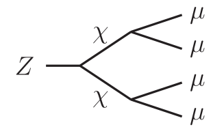
Figure 4: $Z$ decay into four muons mediated by two fakeons $\chi$

Conditions like (7.1), however, do not allow us to sum over the whole phase spaces of the final states, because they include contributions from the regions of the fakeon peaks. At the same time, a nonvanishing resolution $\Delta E$, by conditions (5.4), is bad around the peaks. The processes involving configurations beyond the bounds (7.1) and (5.4) can be investigated phenomenologically, starting from the general properties of fakeons.

7.1 Quantum gravity

Quantum gravity is unitary and renormalizable if a few higher-derivative terms are included (besides the Hilbert-Einstein term and the cosmological term) and the extra degrees of freedom, which are a scalar field $\phi_{\text{infl}}$ and a spin-2 field $\chi_{\mu\nu}$, are quantized as a physical particle (the inflaton) and a spin-2 purely virtual particle, respectively [11]. Primordial cosmology fixes the inflaton mass to $m_{\phi}\simeq 3\cdot 10^{13}$GeV through the spectrum of the scalar fluctuations. The consistency of the fakeon prescription on a nontrivial background gives the ABP bound $m_{\chi}>m_{\phi}/4$ on the fakeon mass $m_{\chi}$ and a sharp prediction on the tensor-to-scalar ratio $r$ ($0.4\lesssim 1000r\lesssim 3$) of the primordial fluctuations [12].

We want to show that the case of $\chi_{\mu\nu}$ is similar to the case of the muon, rather than the one of the $Z$ boson. If we assume that $m_{\chi}$ and $m_{\phi}$ are of the same order, at energies comparable with such masses we have [26]

$$E\simeq m_{\chi}\simeq 3\cdot 10^{13}\text{GeV},\qquad\Gamma_{\chi}\simeq\frac{m_{\chi}^{3}}{M_{\text{Pl}}^{2}}\frac{N_{s}+6N_{f}+12N_{v}}{120}\simeq 4\cdot 10^{2}\text{GeV},$$

where $N_{s}$ is the number of real scalar fields, $N_{f}$ is the number of Dirac fermions plus one half the number of Weyl fermions and $N_{v}$ is the number of gauge bosons of the standard model coupled to quantum gravity.

The key values concerning the $Z$ boson are $\Gamma_{Z}\simeq 2$GeV, $E\simeq m_{Z}\simeq 91$GeV, $\Delta E_{Z}\simeq$ $2\cdot 10^{-3}$GeV (the experimental error on $m_{Z}$). Taking $\left|\Delta m_{Z}^{2}\right|\simeq m_{Z}\Gamma_{Z}$, because they are of the same order, we find $\Delta E_{Z\hskip 0.72229pt\text{min}}/\Delta E_{Z}\simeq 10^{3}$, which violates (4.17), (4.19). Thus, when we need to treat the $Z$ boson around the peak, we must use its dressed propagator. We know that we can do it, because the resummation of the self-energies in the peak region is justified by analyticity.

Now, the fakeon width $\Gamma_{\chi}$ is $2\cdot 10^{2}$ times larger than the $Z$ width $\Gamma_{Z}$. However, the $\chi_{\mu\nu}$ mass $m_{\chi}$ is $3\cdot 10^{11}$ times larger than $m_{Z}$. Using the $Z$ data as reference values, we can assume that a hypothetical scattering process involving $\chi_{\mu\nu}$ particles at energies $E\simeq m_{\chi}$ will have an error $\Delta E_{\chi}\simeq$ $3\cdot 10^{11}\Delta E_{Z}$. Then we expect

$$\frac{\Delta E_{\chi\hskip 0.72229pt\text{min}}}{\Delta E_{\chi}}\simeq 10^{-5},$$ (7.2)

which fulfills (4.17)-(4.19). This is a situation where we do not need to resum the series into (5.2): we can just use the tree-level propagator (2.5) for $\chi_{\mu\nu}$.

As we have anticipated, the situation is similar to the one of the muon, since $m_{\chi}\gg\Delta E_{\chi}\gg\Gamma_{\chi}/2,\Delta E_{\chi\hskip 0.72229pt\text{min}}$. The result depends on $\Delta E_{\chi}$ very little. Precisely, the first propagator of (5.2) around $p^{2}-m^{2}$ ($m^{2}$ being now $m_{\chi}^{2}$) is

$$\frac{iZ_{\chi}(p^{2}-m_{\chi}^{2})}{(p^{2}-m_{\chi}^{2})^{2}+m_{\text{ph}}^{2}\Delta E_{\chi}^{2}}\left[1+\frac{(p^{2}-m_{\chi}^{2})(\Delta m_{\chi}^{2}-im_{\text{ph}}\Gamma_{\chi})}{(p^{2}-m_{\chi}^{2})^{2}+m_{\text{ph}}^{2}\Delta E_{\chi}^{2}}+\cdots\right]$$ (7.3)

$$\sim \mathcal{P}\frac{iZ_{\chi}}{p^{2}-m_{\chi}^{2}}+iZ_{\chi}\pi\delta(p^{2}-m_{\chi}^{2})\frac{(\Delta m_{\chi}^{2}-im_{\text{ph}}\Gamma_{\chi})}{2m_{\text{ph}}\Delta E_{\chi}}+\cdots,$$

having used

$$\lim_{\epsilon\rightarrow 0}\frac{\epsilon x^{2}}{(x^{2}+\epsilon^{2})^{2}}=\lim_{\epsilon\rightarrow 0}\frac{\epsilon^{3}}{(x^{2}+\epsilon^{2})^{2}}=\frac{\pi}{2}\delta(x).$$ (7.4)

Unless we can measure corrections such as (7.2), we can take $\Delta m_{\chi}^{2}$ and $\Gamma_{\chi}$ to $0$, which gives a propagator equal to $i$ times the principal value of $Z_{\chi}/(p^{2}-m_{\chi}^{2})$.

For a better comparison, let us analyze the muon itself, where

$$\Gamma_{\mu}\sim 10^{-19}\text{GeV},\qquad\Delta E_{\mu}\sim 10^{-9}\text{GeV},\qquad\frac{\Gamma_{\mu}}{2\Delta E_{\mu}}\sim 10^{-10},$$

$\Delta E_{\mu}$ being the error on the muon mass. Using formula (4.20) with $\tilde{\epsilon}\rightarrow 2m_{\text{ph}}\Delta E$, together with (7.4), we find

$$\Omega_{\mu\hskip 0.72229pt\text{particle}}\simeq\pi Z\delta(p^{2}-m_{\text{ph}}^{2})\left(1-\frac{\Gamma_{\mu}}{2\Delta E_{\mu}}\right)+\cdots.$$

Unless we can detect corrections $\sim 10^{-10}$, we can ignore the muon width altogether in its propagator, as is normally done.

If some day we will be able to study scattering processes in quantum gravity at energies around $10^{13}$GeV with enough precision to test corrections as small as (7.2), we will see effects such as those of formula (7.3).

7.2 Collider physics

If lighter fakeons exist in nature and have an observable impact in collider physics, a phenomenological description of the nonperturbative effects activated in the peak region may be useful.

We concentrate on the first formula of (5.2), since the second one can be seen as a particular case of it with $\Delta m^{2}=0$, $\tilde{m}=m=m_{\text{ph}}$. Consider the resummed propagators (5.2), with the first condition (5.4). We cannot take $\Delta E$ to zero there, otherwise (5.4) is violated. The simplest possibility is to consider the “minimum uncertainty propagator”, which is the one with $\Delta E=\Delta E_{\text{min}}$. Is this an acceptable, $\Delta E$-independent phenomenological fakeon propagator? The answer is no, because its classical limit $\Delta m^{2},\Gamma\rightarrow 0$ is proportional to

$$\lim_{\varepsilon\rightarrow 0}\frac{ix}{x^{2}+2i\varepsilon\mathrm{e}^{i\theta}x+\varepsilon^{2}}=\mathcal{P}\frac{i}{x}+\frac{\pi\mathrm{e}^{i\theta_{0}}}{\sqrt{1+\mathrm{e}^{2i\theta_{0}}}}\delta(x),\qquad x=\frac{p^{2}-m^{2}}{m_{\text{ph}}^{2}},$$ (7.5)

where $\theta=\arcsin(\Delta m^{2}/(2m_{\text{ph}}\Delta E_{\text{min}}))$, $\varepsilon=\Delta E_{\text{min}}/m_{\text{ph}}$ and $\theta_{0}$ is the classical limit of $\theta$. Since $\Gamma>0$, the angle $\theta$ satisfies $|\theta|<\pi/2$. Moreover, assuming that $\Delta m^{2}$ and $\Gamma$ are of the same order, we also have $|\theta_{0}|<\pi/2$. The limit (7.5) can be proved by studying the even and odd parts separately and acting on arbitrary test functions.

The result is not purely virtual, because the term proportional to $\delta(x)$ signals a nontrivial on-shell contribution. The reason why the coefficient of $\delta(x)$ is nonvanishing is that the classical limit is incompatible with the equality $\Delta E=\Delta E_{\text{min}}$, because $\Delta E_{\text{min}}$ tends to zero, but the resolution $\Delta E$ does not change in that limit.

The correct classical limit amounts to take $\Delta m^{2},\Gamma\rightarrow 0$ first and then $\Delta E\rightarrow 0$, which indeed gives the principal value. Moreover, by (5.4) $\Delta E$ should be strictly larger than $\Delta E_{\text{min}}$, because $\Delta E=\Delta E_{\text{min}}$ does not belong to the convergence region.

Having learned that $\Delta E=\Delta E_{\text{min}}$ is not a good phenomenological assumption, a better proposal that complies with the requirements just outlined is

$$\Delta E=\gamma\Delta E_{\text{min}}\left(\frac{m_{\text{ph}}}{\Delta E_{\text{min}}}\right)^{\delta},\qquad\gamma>0,\qquad 0<\delta<1.$$ (7.6)

The constants $\gamma$ and $\delta$ may be thought as the remnants of the interaction with the experimental setup, or due to nonperturbative effects. Then from (5.2) we have the effective propagator

$$\hat{P}_{\chi}\simeq\frac{iZ(p^{2}-m^{2})}{(p^{2}-m^{2})(p^{2}-m_{\text{ph}}^{2}+im_{\text{ph}}\Gamma)+\gamma^{2}m_{\text{ph}}^{2+2\delta}\Delta E_{\text{min}}^{2-2\delta}},$$ (7.7)

which has the correct classical limit, since

$$\lim_{\varepsilon\rightarrow 0}\frac{ix}{x^{2}+2i\varepsilon\mathrm{e}^{i\theta}x+\gamma^{2}\varepsilon^{2-2\delta}}=\mathcal{P}\frac{i}{x}.$$

This equality can be proved as before.

Formula (7.7) behaves correctly away from the peak, where it approximates the Breit-Wigner formula

$$\hat{P}_{\chi}\simeq\frac{iZ}{p^{2}-m_{\text{ph}}^{2}-im_{\text{ph}}\Gamma}.$$ (7.8)

Presumably, the medium value $\delta=1/2$ is sufficiently accurate. The plot of the real part of (7.7) is shown in fig. 5 (for $\delta=1/2$, $Z=1$, $m_{\text{ph}}=1$, $\Gamma=1/4$, $\Delta m^{2}=1/8$, and for two choices of $\gamma$: $\gamma=1$ and $\gamma=1/2$). For comparison, we include the plot of a Breit-Wigner peak for a standard particle with the same width $\Gamma$ and the same $\Delta m^{2}$. The fakeon plot better “fills” the Breit-Wigner one for lower values of $\gamma$. At $\Delta m^{2}=0$ the two fakeon bumps are symmetric with respect to the vertical line.

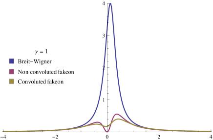
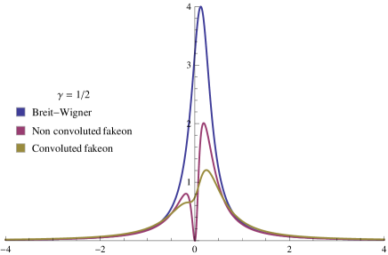
Figure 5: Non-convoluted and convoluted fakeon plots with $\gamma=1$ and $\gamma=1/2$, compared to the Breit-Wigner plot of a standard particle with the same width $\Gamma$ and the same $\Delta m^{2}$

If $\Delta E$ is interpreted as an uncertainty or an experimental error, it may be more accurate to consider the convolution

$$\tilde{P}_{\chi}(x)=\frac{m_{\text{ph}}\Delta E}{\pi}\int_{-\infty}^{+\infty}\mathrm{d}y\frac{\hat{P}_{\chi}(x-y)}{y^{2}+m_{\text{ph}}^{2}\Delta E^{2}},$$

where the expression (7.7) is seen as a function $\hat{P}_{\chi}(x)$ of $x$. The convoluted dressed propagator is also shown in fig. 5.

We see that, in general, the fakeon plot is suppressed with respect to the one of a standard particle. This is not surprising, given the nature of a fake particle. The three plots superpose as soon as we move away from the peak region.

More generally, we can have an $x$-dependent factor $\gamma$ in formula (7.6), such as

$$\gamma(x^{2})=\gamma_{0}\exp\left(-\sigma\frac{x^{2}m_{\text{ph}}}{\Delta E_{\text{min}}}\right),$$ (7.9)

where $\gamma_{0}$ and $\sigma$ are positive constants, so that $\Delta E$ practically vanishes away from the peak and the Breit-Wigner expression (7.8) is reached more rapidly. An expression like (7.9) contains essential singularities in the couplings and could be originated by nonperturbative effects. With such a $\gamma$ we can extend (7.6) to $\delta=0$.

Following the line of thinking that leads to (7.7), we can search for phenomenological formulas for ghosts as well. If we take, for example,

$$\Delta E=\gamma(x^{2})\frac{\Gamma}{2},\qquad\gamma(x^{2})>0,\text{\quad}\gamma(0)>1,\quad\gamma(\infty)=0,$$

where $\gamma(x^{2})$ can be of the form (7.9), we find, from (6.3),

$$\hat{P}_{\phi}\simeq-\frac{iZ}{p^{2}-m_{\text{ph}}^{2}+im_{\text{ph}}\Gamma(\gamma(x^{2})-1)},$$ (7.10)

which has the correct classical limit, since

$$-\lim_{\varepsilon\rightarrow 0}\frac{i}{x+i\varepsilon(\gamma(x^{2})-1)}=-i\mathcal{P}\frac{1}{x}-\pi\delta(x).$$

Formula (7.10) also behaves correctly away from the peak, where $\gamma(x^{2})$ is negligible.

8 Comparison between the peak uncertainty and the violation of microcausality

Fakeons are responsible for the violation of microcausality [26, 7], which prevents predictions for time intervals shorter than $\tau\equiv 1/m_{\chi}$. This means that the theory can be tested only a posteriori, after a delay $\tau$. In this section we compare the violation of microcausality to the peak uncertainty of formula (5.4), which codifies the impossibility to get too close to the fakeon peak. We find that, although the two have a common origin, they are essentially different.

The violation of microcausality is associated with the intrinsic nonlocal nature of the fakeon projection. Its effects can be appreciated in coordinate space. We can illustrate them with an example taken from ref. [7]. Consider the Lagrangian

$$\mathcal{L}(x,Q,t)=\frac{m}{2}\dot{x}^{2}-m\dot{x}\dot{Q}+\frac{m}{2\tau^{2}}Q^{2}+xF_{\text{ext}}(t),$$

where $x$ is the coordinate of a physical particle, $Q$ is the one of a purely virtual particle, $m$ and $\tau$ are constants and $F_{\text{ext}}(t)$ is a time-dependent external force. The equations of motion give

$$\ddot{x}=-\frac{Q}{\tau^{2}},\qquad m\ddot{Q}+\frac{m}{\tau^{2}}Q=-F_{\text{ext}}(t).$$

Since $Q$ is a fakeon, its equation admits the unique solution

$$mQ=-\mathcal{P}\frac{\tau^{2}}{1+\tau^{2}\frac{\mathrm{d}^{2}}{\mathrm{d}t^{2}}}F_{\text{ext}}(t)=-\frac{\tau}{2}\int_{-\infty}^{\infty}\mathrm{d}u\hskip 0.72229ptF_{\text{ext}}(t-u)\sin\left(\frac{|u|}{\tau}\right),$$

given by the fakeon prescription. Inserting this expression into the equation of $x$, we obtain

$$m\ddot{x}=\frac{1}{2\tau}\int_{-\infty}^{\infty}\mathrm{d}u\hskip 0.72229ptF_{\text{ext}}(t-u)\sin\left(\frac{|u|}{\tau}\right).$$ (8.1)

The integral appearing on the right-hand side receives contributions from the external force in the past as well as in the future. The amount of future effectively contributing is

$$\left|\Delta u\right|\simeq\tau,$$ (8.2)

due to the oscillating behavior of $1/(2\tau)\sin(|u|/\tau)$, and disappears for $\tau\rightarrow 0$, since $\lim_{\tau\rightarrow 0}1/(2\tau)\sin(|u|/\tau)=\delta(u)$. Thus, (8.2) encodes the fuzziness due to the violation of microcausality. It implies that we cannot make predictions for time intervals shorter than $\tau$. However, we can, in principle, check (8.1) a posteriori, if we manage to measure $x(t)$ and $F_{\text{ext}}(t)$ independently.

This example shows that the violation of microcausality due to fakeons does not need a nonvanishing width. The key quantity encoding it is the fakeon mass $m_{\chi}$ (which is $1/\tau$ in the toy model just considered). For this reason, the violation survives the classical limit.

The peak uncertainty, instead, is encoded in the radiative corrections $\Gamma_{\chi}$ and possibly $\Delta m_{\chi}^{2}$, so it disappears in the classical limit. It concerns the energy and implies that we cannot get too close to $E\sim m_{\chi}$ in the channels mediated by fakeons. It does not prevent predictions on processes occurring at higher energies. If light fakeons exist in nature, it should be possible to detect the peak uncertainty experimentally. Instead of seeing a resonance, as we expect for a normal particle, we should see one or two bumps, with shapes that depend on the experimental setup in a way that may be difficult, or impossible, to predict.

While the violation of microcausality is always present, being associated with the fakeon mass, it is possible to have no peak uncertainty (5.8). It happens when the dressed propagator is the second of (5.2) and the fakeon width $\Gamma_{\chi}$ vanishes, as in the models of ref. [9].

These arguments show that there is no direct correspondence between the peak uncertainty (5.8) and the violation of microcausality.

9 Conclusions

We have studied the dressed propagators of purely virtual particles and compared the results with those of physical particles and ghosts, pointing out several nontrivial issues that are commonly ignored. For example, the usual dressed propagator is unable to explain the experimental observation of long-lived unstable particles, like the muon. The difficulty can be overcome by introducing the energy resolution $\Delta E$ of the experimental setup. The need of $\Delta E$ is explained by the usual energy-time uncertainty relation, which implies that it is impossible to observe an unstable particle with infinite resolving power on the energy.

The expansions of the dressed propagators of physical particles, fake particles and ghosts differ by infinite series of contact terms, which cannot be summed into well-defined mathematical distributions. If we insist in trusting the formal resummations, we obtain physical absurdities on new types. Problematic sums also appear with physical particles, when we want to distinguish their observation from the observation of their decay products.

The problems originate from the resummation of the self-energies in the peak region, which lies outside the convergence domain of the geometric series. In the case of physical particles, analyticity allows us to extend the dressed propagator from the convergence region to the entire domain of external momenta, provided we treat the observation of the particle and the observation of its decay products as a whole. Analyticity is helpless in the other cases. In particular, it is helpless in the cases of fake particles and ghosts, where the formal sums cannot be trusted. All the truncations are equally inadequate there, since the terms of the expansion never decrease. This means that the problems become nonperturbative, when we approach the peak.

In the case of fakeons, these facts point to a new type of uncertainty relation, a “peak uncertainty” $\Delta E\gtrsim\Delta E_{\text{min}}=\Gamma/2$, which constrains our observations. Knowing the very nature of the fakeon, it is not surprising that we cannot approach its peak too closely, since, by definition, a purely virtual particle refuses to be brought to reality.

Ultimately, the quantization prescription cannot be washed away by the resummation. There is always a region where the true nature of the particle we are studying (physical, fake or ghost) makes the difference.

The regime $\Delta E\gg\Gamma/2$ applies to quantum gravity and situations like the one of the muon, where the resummation is unnecessary. The regime $\Delta E\ll\Gamma/2$ applies to collider physics and situations like the one of the $Z$ boson. We have provided phenomenological candidates for the dressed propagators close to the peaks, to describe what the nonperturbative effects might look like there.

The peak uncertainty has no direct relation with the violation of microcausality, also due to fakeons.

Acknowledgments

We are grateful to U. Aglietti, D. Comelli, E. Gabrielli, L. Marzola, M. Piva and M. Raidal for helpful discussions. We thank the National Institute of Chemical Physics and Biophysics (NICPB), Tallinn, Estonia, for hospitality during the early stage of this work.

Appendices

A Alternative formal resummation for purely virtual particles

In this appendix we derive the alternative formula (2.8) for the formal dressed propagator of a purely virtual particle. The crucial point is the role of the infinitesimal width $\epsilon$. Consider the identities

$$\sum_{n=0}^{\infty}(a+b)^{n} = \frac{1}{1-a}\sum_{n=0}^{\infty}\left(\frac{b}{1-a}\right)^{n}=\frac{1}{1-a-b},$$

$$\sum_{n=0}^{\infty}(a+b+c)^{n} = \frac{1}{1-a-b}\sum_{n=0}^{\infty}\left(\frac{c}{1-a-b}\right)^{n}=\frac{1}{1-a-b-c},$$ (A.1)

which hold perturbatively in $a$, $b$ and $c$. If we apply them to the sum that appears in (2.6), with

$$a=-i(1-Z^{-1})(p^{2}-m^{2})P_{\chi},\quad b=-iZ^{-1}\Delta m^{2}P_{\chi},\quad c=-Z^{-1}m_{\text{ph}}\Gamma P_{\chi},$$

we can first sum the powers of $1-Z^{-1}$, then the powers of $\Delta m^{2}$ and finally the powers of $\Gamma$. This gives us the possibility to treat them differently, because they are not on an equal footing with respect to the problems that we discuss in the paper.

For example, the powers of $1-Z^{-1}$ can be summed with no difficulty, because $Z$ is just the overall normalization. They give

$$P_{\chi}(p^{2},m^{2},\epsilon)\frac{1}{1-a}=\frac{iZ(p^{2}-m^{2})}{(p^{2}-m^{2})^{2}+\tilde{\epsilon}^{2}}=ZP_{\chi}(p^{2},m^{2},\tilde{\epsilon})\underset{\tilde{\epsilon}\rightarrow 0}{\rightarrow}\mathcal{P}\frac{iZ}{p^{2}-m^{2}}.$$

In this derivation it does not really matter whether we remove $\epsilon$ term by term or after the sum.

If we proceed with the first line of (A.1), we need to calculate

$$P_{\chi}(p^{2},m^{2},\epsilon)\frac{1}{1-a}\sum_{n=0}^{\infty}\frac{b^{n}}{(1-a)^{n}}=ZP_{\chi}(p^{2},m^{2},\tilde{\epsilon})\sum_{n=0}^{\infty}\left[-i\Delta m^{2}P_{\chi}(p^{2},m^{2},\tilde{\epsilon})\right]^{n}.$$

Taking $\epsilon$ to zero term-by-term, we get powers of the Cauchy principal value. The coincidence-splitting method (see [6] and appendix C) amounts to define such powers by starting from non coincident singularities and using the identity (C.1). Then we find

$$iZ\sum_{n=0}^{\infty}\frac{(-\Delta m^{2})^{n}}{n!}\mathcal{P}^{(n)}\frac{1}{p^{2}-m^{2}}=\mathcal{P}\frac{iZ}{p^{2}-m_{\text{ph}}^{2}}\underset{\tilde{\epsilon}\rightarrow 0}{\leftarrow}\frac{iZ(p^{2}-m_{\text{ph}}^{2})}{(p^{2}-m_{\text{ph}}^{2})^{2}+\tilde{\epsilon}^{2}}=ZP_{\chi}(p^{2},m_{\text{ph}}^{2},\tilde{\epsilon})$$ (A.2)

where $\mathcal{P}^{(n)}$ is the $n$-th derivative of the principal value. We have restored $\tilde{\epsilon}$ in the last two expressions.

As far as the powers of $\Gamma$ are concerned, we cannot resum them with $\tilde{\epsilon}=0$, as shown in subsection 3.3. If we use the second line of (A.1), we obtain

$$\hat{P}_{\chi}\simeq ZP_{\chi}(p^{2},m_{\text{ph}}^{2},\tilde{\epsilon})\sum_{n=0}^{\infty}\left[-m_{\text{ph}}\Gamma P_{\chi}(p^{2},m_{\text{ph}}^{2},\tilde{\epsilon})\right]^{n}$$

and the sum gives formula (2.8).

B Singular distributions

A distribution is a continuous linear functional on the space of test functions, which are the infinitely differentiable functions with compact support. In this appendix we show that $\Delta_{\hat{\Gamma}}(x)$, defined in formula (3.4), is not a distribution. Let us start from the truncated sums

$$\Delta_{\hat{\Gamma}}^{N}(x)\equiv\sum_{n=0}^{N}\frac{(-\hat{\Gamma}^{2})^{n}}{(2n)!}\delta^{(2n)}(x)$$

and check their actions on the function $g(x)=1/(x^{2}+\hat{\Gamma}^{2})$. Since

$$\Delta_{\hat{\Gamma}}^{N}g\equiv\int_{-\infty}^{+\infty}\mathrm{d}x\hskip 0.72229pt\Delta_{\hat{\Gamma}}^{N}(x)g(x)=\frac{N+1}{\hat{\Gamma}^{2}},$$

the limit $N\rightarrow\infty$ does not converge. We reach the same conclusion on the test function

$$\hat{g}(x)=\left\{\begin{tabular}[]{l}$g(x)\mathrm{e}^{-\frac{R^{2}}{(R^{2}-x^{2})}}$ for $|x|<R,$\\ 0 for $|x|\geqslant R,$\end{tabular}\right.$$

with $\hat{\Gamma}<R$, where $R>0$ is some radius. This proves that the sequence of distributions $\Delta_{\hat{\Gamma}}^{N}$ does not converge to a distribution.

Now, consider the functions

$$f_{n}(x)=\frac{x-\frac{1}{n}}{\left(x-\frac{1}{n}\right)^{2}+\hat{\Gamma}^{2}}.$$ (B.1)

The sum of (3.4) converges for $\hat{\Gamma}<1/(2n)$, where it gives

$$\Delta_{\hat{\Gamma}}f_{n}\equiv\int_{-\infty}^{+\infty}\mathrm{d}x\hskip 0.72229pt\Delta_{\hat{\Gamma}}(x)f_{n}(x)\equiv-\frac{n(1+2n^{2}\hat{\Gamma}^{2})}{1+4n^{2}\hat{\Gamma}^{2}}.$$ (B.2)

It does not converge for $\hat{\Gamma}\geqslant 1/(2n)$. If, given $n$, we define $\Delta_{\hat{\Gamma}}f_{n}$ to be the right-hand side of (B.2) everywhere, by analytic continuation from the region $0<\hat{\Gamma}<1/(2n)$, we find another problem: $f_{n}(x)$ tends to $\hskip 0.72229ptf_{\infty}(x)=x/(x^{2}+\hat{\Gamma}^{2})$ for $n\rightarrow\infty$, but the right-hand side of (B.2) explodes.

The functions (B.1) are not test functions, but the test functions

$$\hat{f}_{n}(x)=\left\{\begin{tabular}[]{l}$f_{n}(x)\mathrm{e}^{-\frac{R^{2}}{(R^{2}-x^{2})}}$ for $|x|<R,$\\ 0 for $|x|\geqslant R,$\end{tabular}\right.$$

lead to the same conclusions for $\hat{\Gamma}<R$. Precisely, $\Delta_{\hat{\Gamma}}\hat{f}_{n}$ is equal to the right-hand side of (B.2) times $\mathrm{\exp}(-R^{2}/(R^{2}+\hat{\Gamma}^{2}))$, so the product still blows up for $n\rightarrow\infty$. This means, again, that $\Delta_{\hat{\Gamma}}(x)$ is not a continuous linear functional, i.e., not a distribution.

C Coincidence-splitting method

In this appendix we explain how to define the products of principal values and delta functions by means of the coincidence-splitting method or, when necessary, its symmetrized version. The idea is to treat coincident singularities as the limits of distinct ones.

First observe that the powers of $\delta(x)$ higher than one are set to zero by this method. The powers of the Cauchy principal value were considered in [25], where it was proved that

$$\lim_{\delta_{i}\rightarrow 0}\mathcal{P}\prod\limits_{i=1}^{n+1}\frac{1}{x-\delta_{i}}=\frac{(-1)^{n}}{n!}\mathcal{P}^{(n)}\frac{1}{x},$$ (C.1)

(the parameters $\delta_{i}$ being different from one another).

The product of one delta function times powers of the principal value gives

$${\text{s}}\!\!\lim_{\delta_{i}\rightarrow 0}\delta(x-\delta_{1})\mathcal{P}\prod\limits_{i=2}^{n+1}\frac{1}{x-\delta_{i}}=\frac{(-1)^{n}}{(n+1)!}\delta^{(n)}(x),$$ (C.2)

where “slim” means that the expression must be symmetrized in $\delta_{i}$, $i=1,\ldots n+1$ before taking the limit. The identity (C.2) can be proved by acting on a test function $f(x)$. We write

$${\text{s}}\!\!\lim_{\delta_{i}\rightarrow 0}\int_{-\infty}^{+\infty}\mathrm{d}x\hskip 0.72229ptf(x)\delta(x-\delta_{1})\mathcal{P}\prod\limits_{i=2}^{n+1}\frac{1}{x-\delta_{i}}=\frac{1}{n+1}\lim_{\delta_{i}\rightarrow 0}\sum_{j=1}^{n+1}f(\delta_{j})\prod\limits_{i=1,i\neq j}^{n+1}\frac{1}{\delta_{j}-\delta_{i}},$$

then Taylor expand $f(x)$ around zero and finally use the formula

$$\sum_{j=1}^{n+1}\delta_{j}^{k}\prod\limits_{i=1,i\neq j}^{n+1}\frac{1}{\delta_{j}-\delta_{i}}=\left\{\begin{tabular}[]{l}$0\qquad$for $k<n$\\ $1\qquad$for $k=n$\\ polynomial of $\delta_{j}$ for $k>n.$\end{tabular}\right.$$

The result is $f^{(n)}(0)/(n+1)!$, in agreement with (C.2).

We can use these results, for example, to study the expansions of $\Omega_{\varphi\hskip 0.72229pt\text{particle}}$ and $\Omega_{\varphi\hskip 0.72229pt\text{decay}}$ by letting $\epsilon$ tend to zero term by term. The diagrams listed in the first and second lines of fig. 3 give

$$2\Omega_{\varphi\hskip 0.72229pt\text{particle}} = \sum_{k=0}^{\infty}(i\Sigma^{\ast}P_{\varphi}^{\ast})^{k}(P_{\varphi}+P_{\varphi}^{\ast})\sum_{n=0}^{\infty}(-i\Sigma P_{\varphi})^{n},$$

$$2\Omega_{\varphi\hskip 0.72229pt\text{decay}} = P_{\varphi}^{\ast}\sum_{k=0}^{\infty}(i\Sigma^{\ast}P_{\varphi}^{\ast})^{k}(-2\text{Im}[\Sigma])\sum_{n=0}^{\infty}(-i\Sigma P_{\varphi})^{n}P_{\varphi},$$ (C.3)

where $P_{\varphi}+P_{\varphi}^{\ast}$ is the cut propagator and $2$Im$[\Sigma]=-i\Sigma+(-i\Sigma)^{\ast}$ is the cut bubble diagram. We apply the approximation (2.3) with $\Delta m^{2}=0$, $Z=1$, to focus on the powers of $\Gamma$. Using $m^{2}P_{\varphi}=\pi\delta(x)+i\mathcal{P}(1/x)$, $P_{\varphi}+P_{\varphi}^{\ast}=$ $2\pi\delta(x)/m^{2}$ and $2$Im$[\Sigma]=-2m^{2}\hat{\Gamma}$, where $x=(p^{2}-m^{2})/m^{2}$ and $\hat{\Gamma}=\Gamma/m$, and dealing with the products of delta functions and principal values by means of formulas (C.1) and (C.2), we obtain

$$\Omega_{\varphi\hskip 0.72229pt\text{particle}} \rightarrow \frac{\pi}{m^{2}}\sum_{n=0}^{\infty}\frac{(-\hat{\Gamma}^{2})^{n}}{(2n+1)!}\delta^{(2n)}(x),$$

$$\Omega_{\varphi\hskip 0.72229pt\text{decay}} \rightarrow \frac{1}{m^{2}\hat{\Gamma}}\sum_{n=0}^{\infty}\frac{(-\hat{\Gamma}^{2})^{n+1}}{(2n+1)!}\mathcal{P}^{(2n+1)}\frac{1}{x}+\frac{\pi}{m^{2}}\sum_{n=0}^{\infty}\frac{2n(-\hat{\Gamma}^{2})^{n}}{(2n+1)!}\delta^{(2n)}(x).$$ (C.4)

Taken separately, these expressions are not well-defined distributions. However, their sum is. Indeed, formula (3.5) gives

$$\Omega_{\varphi\hskip 0.72229pt\text{particle}}+\Omega_{\varphi\hskip 0.72229pt\text{decay}}\rightarrow\frac{1}{m^{2}}\frac{\hat{\Gamma}}{x^{2}+\hat{\Gamma}^{2}},$$ (C.5)

which is the expected Breit-Wigner function.

References

- [1] R.E. Cutkosky, Singularities and discontinuities of Feynman amplitudes, J. Math. Phys. 1 (1960) 429.
- [2] M. Veltman, Unitarity and causality in a renormalizable field theory with unstable particles, Physica 29 (1963) 186.
- [3] G. ’t Hooft, Renormalization of massless Yang-Mills fields, Nucl. Phys. B 33 (1971) 173; G. ’t Hooft, Renormalizable Lagrangians for massive Yang-Mills fields, Nucl. Phys. B 35 (1971) 167.
- [4] G. ’t Hooft and M. Veltman, Diagrammar, CERN report CERN-73-09.
- [5] M. Veltman, Diagrammatica. The path to Feynman rules (Cambridge University Press, New York, 1994).
- [6] D. Anselmi, Diagrammar of physical and fake particles and spectral optical theorem, J. High Energy Phys. 11 (2021) 030, 21A5 Renormalization.com and arXiv: 2109.06889 [hep-th].
- [7] D. Anselmi, Fakeons, microcausality and the classical limit of quantum gravity, Class. and Quantum Grav. 36 (2019) 065010, 18A4 Renormalization.com and arXiv:1809.05037 [hep-th].
- [8] D. Anselmi, Fakeons and Lee-Wick models, J. High Energy Phys. 02 (2018) 141, 18A1 Renormalization.com and arXiv:1801.00915 [hep-th].
- [9] D. Anselmi, K. Kannike, C. Marzo, L. Marzola, A. Melis, K. Müürsepp, M. Piva and M. Raidal, Phenomenology of a fake inert doublet model, J. High Energy Phys. 10 (2021) 132, 21A3 Renormalization.com and arXiv:2104.02071 [hep-ph].
- [10] D. Anselmi, K. Kannike, C. Marzo, L. Marzola, A. Melis, K. Müürsepp, M. Piva and M. Raidal, A fake doublet solution to the muon anomalous magnetic moment, Phys. Rev. D 104 (2021) 035009, 21A4 Renormalization.com and arXiv:2104.03249 [hep-ph].
- [11] D. Anselmi, On the quantum field theory of the gravitational interactions, J. High Energy Phys. 06 (2017) 086, 17A3 Renormalization.com and arXiv: 1704.07728 [hep-th].
- [12] D. Anselmi, E. Bianchi and M. Piva, Predictions of quantum gravity in inflationary cosmology: effects of the Weyl-squared term, J. High Energy Phys. 07 (2020) 211, 20A2 Renormalization.com and arXiv:2005.10293 [hep-th].
- [13] G. J. van Oldenborgh and J. A. M. Vermaseren, New Algorithms for One Loop Integrals, Z. Phys. C 46 (1990) 425. J. Kublbeck, M. Bohm, and A. Denner, Feyn Arts: Computer Algebraic Generation of Feynman Graphs and Amplitudes, Comput. Phys. Commun. 60 (1990) 165; A. Denner, Techniques for calculation of electroweak radiative corrections at the one loop level and results for W physics at LEP-200, Fortsch. Phys. 41 (1993) 307 and arXiv:0709.1075; T. Hahn, Loop calculations with FeynArts, FormCalc, and LoopTools, Acta Phys. Polon. B30 (1999) 3469 and arXiv:hep-ph/9910227; T. Hahn, Generating Feynman diagrams and amplitudes with FeynArts 3, Comput. Phys. Commun. 140 (2001) 418 and arXiv:hep-ph/0012260; A. Alloul, N. D. Christensen, C. Degrande, C. Duhr and B. Fuks, FeynRules 2.0 - A complete toolbox for tree-level phenomenology, Comput. Phys. Commun. 185 (2014) 2250 and arXiv:1310.1921; H.H. Patel, Package-X: A Mathematica package for the analytic calculation of one-loop integrals, Comput. Phys. Commun. 197 (2015) 276 and arXiv:1503.01469 [hep-ph].
- [14] W. Pauli and F. Villars, On the invariant regularization in relativistic quantum theory. Rev. Mod. Phys. 21 (1949) 434.
- [15] K.S. Stelle, Renormalization of higher derivative quantum gravity, Phys. Rev. D 16 (1977) 953.
- [16] A. Salvio and A. Strumia, Agravity, J. High Energy Phys. 06 (2014) 80 and arXiv:1403.4226 [hep-ph]; A. Salvio and A. Strumia, Agravity up to infinite energy, Eur. Phys. C 78 (2018) 124 and arXiv:1705.03896 [hep-th]; A. Salvio, A. Strumia and H. Veermae, New infra-red enhancements in 4-derivative gravity, Eur. Phys. J. C 78 (2018) 842 and arXiv:1808.07883 [hep-th].
- [17] T.D. Lee and G.C. Wick, Negative metric and the unitarity of the S-matrix, Nucl. Phys. B 9 (1969) 209.
- [18] T.D. Lee and G.C. Wick, Finite theory of quantum electrodynamics, Phys. Rev. D 2 (1970) 1033.
- [19] T.D. Lee, A relativistic complex pole model with indefinite metric, in Quanta: Essays in Theoretical Physics Dedicated to Gregor Wentzel (Chicago University Press, Chicago, 1970), p. 260.
- [20] N. Nakanishi, Lorentz noninvariance of the complex-ghost relativistic field theory, Phys. Rev. D 3 (1971) 811.
- [21] R.E. Cutkosky, P.V Landshoff, D.I. Olive, J.C. Polkinghorne, A non-analytic S matrix, Nucl. Phys. B12 (1969) 281.
- [22] B. Grinstein, D. O’Connell and M.B. Wise, Causality as an emergent macroscopic phenomenon: The Lee-Wick O(N) model, Phys. Rev. D 79 (2009) 105019 and arXiv:0805.2156 [hep-th].
- [23] D. Anselmi, Purely virtual particles versus Lee-Wick ghosts: physical Pauli-Villars fields, finite QED and quantum gravity, to appear in Phys. Rev. D, 22A1 Renormalization.com and arXiv:2202.10483 [hep-th].
- [24] D. Anselmi, The quest for purely virtual quanta: fakeons versus Feynman-Wheeler particles, J. High Energy Phys. 03 (2020) 142, 20A1 Renormalization.com and arXiv:2001.01942 [hep-th].
- [25] D. Anselmi, Fakeons and the classicization of quantum gravity: the FLRW metric, J. High Energy Phys. 04 (2019) 61, 19A1 Renormalization.com and arXiv:1901.09273 [gr-qc].
- [26] D. Anselmi and M. Piva, Quantum gravity, fakeons and microcausality, J. High Energy Phys. 11 (2018) 21, 18A3 Renormalization.com and arXiv:1806.03605 [hep-th].