Susceptibility of Polar Flocks to Spatial Anisotropy

Abstract

We consider the effect of spatial anisotropy on polar flocks by investigating active $q$-state clock models in two dimensions. In contrast to what happens in equilibrium, we find that, in the large-size limit, any amount of anisotropy changes drastically the phenomenology of the rotationally-invariant case, destroying long-range correlations, pinning the direction of global order, and transforming the traveling bands of the coexistence phase into a single moving domain. All this happens beyond a lengthscale that diverges in the $q\to\infty$ limit. A phenomenology akin to that of the Vicsek model can thus be observed in a finite system for large enough values of $q$. We provide a scaling argument which rationalizes why anisotropy has so different effects in the passive and active cases.

Active matter, being made of energy-consuming units, is well known to exhibit spectacular collective behaviors not permitted in equilibrium. Experimental examples include the complex defect dynamics of active nematics Sanchez et al. (2012); Li et al. (2019); Duclos et al. (2020), low Reynolds number turbulence Wensink et al. (2012); Martinez et al. (2020), motility-induced phase separation Buttinoni et al. (2013); Geyer et al. (2019); Van Der Linden et al. (2019) and, perhaps most famously, flocking Cavagna et al. (2010); Bricard et al. (2013); Geyer et al. (2018); Deseigne et al. (2010); Kumar et al. (2014). Although these phenomena appear in complex, usually living, systems, most of our theoretical understanding comes from studying collections of identical active units evolving in pristine environments, often with periodic boundary conditions. Recently acquired evidence suggests, though, that active systems seem to be fundamentally sensitive to quenched and population disorder Chepizhko et al. (2013); Toner et al. (2018a, b); Dor et al. (2019); Duan et al. (2021); Ventejou et al. (2021); Ro et al. (2021), and that even the nature of boundaries can influence bulk properties Dor et al. (2021).

The sensitivity of active systems to anisotropy, in the form of fixed preferred directions in space, remains largely unexplored. A basic result is available in the context of polar flocks, i.e. collections of simple self-propelled particles locally aligning their velocities. In two space dimensions, comparing the Vicsek model (VM) Vicsek et al. (1995) to the active Ising model (AIM) Solon and Tailleur (2013) shows that the symmetry of the order parameter controls the emerging physics. In the VM, the self propulsion dynamics are rotation invariant, i.e., have continuous symmetry, and the ordered phase exhibits scale-free density and order fluctuations Toner and Tu (1995, 1998); Toner et al. (2005); Toner (2012); Mahault et al. (2019). In the AIM, directed motion happens only along two opposite directions, hence the dynamics only has a discrete symmetry, and the correlations are short ranged in the ordered phase. Concomitantly, even though the transition to collective motion is akin to a phase-separation scenario in both the AIM and the VM, their coexistence phases are different Solon et al. (2015a): models in the Vicsek class exhibit microphase separation, typically in the form of a smectic train of traveling dense bands Chaté et al. (2008), whereas the AIM shows a single moving domain and macrophase separation Solon and Tailleur (2015).

The AIM, by restricting directed motion along one dimension, corresponds to an extreme spatial anisotropy. A natural question is then whether polar flocks are affected by weaker forms of anisotropy. In equilibrium, the phenomenology of the 2D XY model—which is the passive counterpart of the VM—is in a sense both robust and sensitive to the discreteness of spins: $q$-state clock models, which break rotational invariance and interpolate between the XY and the Ising models, exhibit a quasi-long-range ordered phase similar to that of the XY model below the BKT transition for $q>4$, but this critical phase gives way to a region of long-range order below some finite temperature that vanishes only when $q\to\infty$ José et al. (1977); Elitzur et al. (1979); Tobochnik (1982); Lapilli et al. (2006); Li et al. (2020). Thus, from the XY viewpoint, a new ordered phase emerges at any $q$, but is marginal, confined to $T=0$, in the $q\to\infty$ limit.

In this Letter, we investigate the susceptibility of polar flocks to weak anisotropy. Using a combination of numerical simulations and analytical arguments, we study $q$-state active clock models and their hydrodynamic theories. We uncover a scenario qualitatively different from the equilibrium one: the phenomenology of the rotationally invariant Vicsek model disappears for any amount of spin anisotropy, leaving only AIM-like phenomenology with short-ranged correlations and macrophase separation. This, however, happens only asymptotically: at fixed $q$, one still observes the Vicsek physics up to a typical scale $\xi_{q}$ that diverges exponentially with $q$, which we estimate using a mean-field theory. Finally, we use a scaling argument which does not depend on mean-field theory, but, rather, only on symmetry, to trace back the fundamental difference with equilibrium to the presence of long-range order in the isotropic active system.

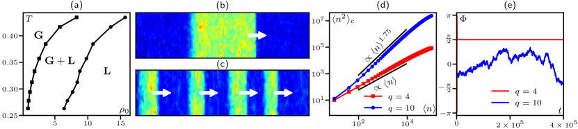
Figure 1: (a) Typical phase diagram in the $(\rho_{0},T)$ plane ($q=4$), Transition lines are defined by the coexisting densities at a given temperature $T=1/\beta$, computed in systems of size $400\times 20$). (b,c): Snapshots of density field in the coexistence phase in a long $800\times 20$ system suitable for the observation of many traveling bands (steady state, $\rho_{0}=10$, $q=4$ in (b), $q=10$ in (c)). (d) Number fluctuations $\langle n^{2}\rangle_{\rm c}$ vs $\langle n\rangle=\rho_{0}\ell^{2}$, the number of particles in a square box of linear size $\ell$ calculated in the liquid phase of square $200\times 200$ systems ($\rho_{0}=10$, $\beta=3.5$). “Giant” anomalous fluctuations are observed for $q=10$, but not for $q=4$. (e) Time series of $\Phi\equiv\arg\langle\mathbf{m}_{k}\rangle_{k}$, the orientation of the global polar order (parameters as in (d)).

Active clock models. Particles $i=1,\ldots,N$ carrying a spin $s_{i}\in\{0,1,\ldots,q-1\}$ reside at the nodes ${\bf R}$ of a square lattice without occupation constraints. They undergo biased diffusion by jumping to neighboring sites with rate $D(1+\varepsilon\mathbf{d}\cdot\mathbf{u}_{i})$ with $\mathbf{d}$ the direction of the jump and $\mathbf{u}_{i}=(\cos\theta_{i},\sin\theta_{i})$ the unit vector along the clock angle $\theta_{i}=2\pi s_{i}/q$. Spins can rotate to the previous or next “hour” $\theta_{i}\pm\tfrac{2\pi}{q}$ at rate

$$w_{i,{\bf R}}=w_{0}\exp\left[\tfrac{\beta}{2\rho_{\bf R}}\mathbf{m}_{\bf R}\cdot(\mathbf{u}_{i}^{\prime}-\mathbf{u}_{i})\right]$$ (1)

where $\rho_{\bf R}$ and $\mathbf{m}_{\bf R}=\sum_{j\in{\bf R}}\mathbf{u}_{j}$ are, respectively the number of particles and the magnetization at site ${\bf R}$ hosting particle $i$, $\mathbf{u}_{i}^{\prime}$ is the new spin direction, and $w_{0}$ is a constant . For $q=2$, one recovers the AIM used in Solon and Tailleur (2015). As shown in SUP , in the isotropic $q\to\infty$ limit, the spin dynamics reduces to the Langevin equation

$$\partial_{t}\theta_{i}=\Omega_{\infty}+\sqrt{2D_{\infty}}\xi_{i}$$ (2)

where $\xi_{i}$ is a Gaussian white noise of unit variance and the torque and rotational diffusivity are given by $\Omega_{\infty}=\frac{4w_{0}\pi^{2}\beta}{q^{2}}\left(\frac{\mathbf{m}_{\bf R}}{\rho_{\bf R}}\cdot\frac{\partial\mathbf{u}_{i}}{\partial\theta_{i}}\right)+O(q^{-3})$ and $D_{\infty}=\frac{4w_{0}\pi^{2}}{q^{2}}+O(q^{-3})$, respectively. In order to have a well-behaved active XY model in the $q\to\infty$ limit, one must thus take $w_{0}\propto q^{2}$. In the following, we set $w_{0}=\tfrac{q^{2}}{4\pi^{2}}$ to fix $D_{\infty}=1$ and choose $D=1$ without loss of generality. For simplicity, we also fix the activity parameter $\varepsilon=0.9$.

The only parameters left to vary, in addition to $q$, are thus the temperature $T=1/\beta$ and the global density $\rho_{0}=N/(L_{x}L_{y})$, where $L_{x}$ and $L_{y}$ define a rectangular domain with periodic boundary conditions. For numerical efficiency, we use parallel updating, first performing on-site spin rotations, then biased jumps.

Phase diagrams in the $(\rho_{0},T)$ plane obtained for a given $q$ value all resemble those of the AIM or VM: the disordered gas present at high $T$ and/or low $\rho_{0}$ is separated from the low-$T$/high-$\rho_{0}$ polarly-ordered liquid by a coexistence phase (Fig. 1(a)). The liquid and coexistence phases both have a finite global magnetization $m\equiv|\langle\mathbf{m}_{\bf R}\rangle_{\bf R}|$. However, at fixed system size, they display AIM-like or VM-like properties depending on $q$: For large-enough $q$, one observes giant number fluctuations in the polar liquid and microphase separation as for the Vicsek model (Fig. 1(c,d)). At lower $q$ values, on the contrary, the liquid has normal fluctuations and the system phase separates into a single moving domain (Fig. 1(b,d)). The global direction of order $\Phi\equiv\arg\langle\mathbf{m}_{\bf R}\rangle_{\bf R}$ also behaves differently in the liquid phase: it wanders slowly at high $q$, whereas it is pinned at one of the clock angles at low $q$ (Fig. 1(e)).

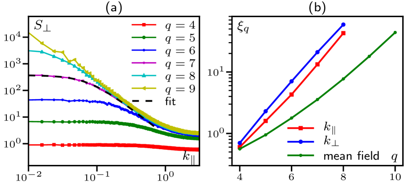
Figure 2: (a) Liquid phase: $S_{\perp}(\mathbf{q})=\langle m_{\perp}(\mathbf{k})m_{\perp}(-\mathbf{k})\rangle$ vs $\mathbf{k}=(k_{\|},0)$ for various $q$ values ($\rho_{0}=5.5$, $\beta=4$, system size $800\times 800$). For $q=7$ we show the function $\alpha/(1+(\xi k_{\|})^{2})$ with $\alpha$ and $\xi$ as fitted parameters. (b) Crossover length $\xi_{q}$ in the liquid phase extracted from (i) fits of $S_{\perp}(\mathbf{k})$ as shown in (a) for $q=7$ for $\mathbf{k}=(k_{\|},0)$ and $\mathbf{k}=(0,k_{\perp})$ (red and blue curves, respectively, same parameters as in (a)) and (ii) the mean-field prediction derived from Eq. (5) (green curve).

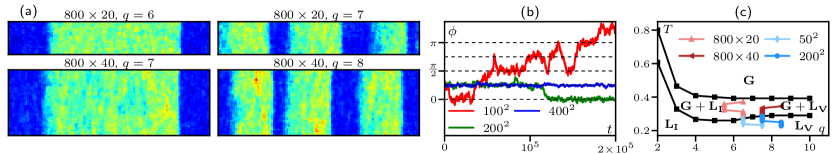
Figure 3: Transition from the active Ising to the Vicsek behavior as system size increases. (a): Snapshots of the density obtained after a long time $t=5\times 10^{5}$ starting from a large ordered band. The transition is shifted to larger $q$ as $L$ increases. Same color code as in Fig. 1. $\beta=3.2$, $\rho_{0}=5.5$. (b): Direction of global order showing a transition between unpinned and pinned as system size increases. The dashed lines indicate the hours of the clock. $\beta=4$, $\rho_{0}=5.5$, $q=8$. (c): Phase diagram in the $q-T$ plane at $\rho_{0}=5.5$. The line between macro- ($G+L_{I}$) and micro-phase separation ($G+L_{V}$) is defined as the transition between a single and multiple bands after time $t=10^{6}$ at the system size indicated in the legend. The line separating the two liquids ($L_{I}$ and $L_{V}$) is defined as the transition between pinned and unpinned order parameter orientation after time $t=10^{5}$.

The results presented in Fig. 1 seem to suggest that active clock models have different behavior at $q=4$ and $q=10$, similar to the differences between the AIM and the VM. In fact this is only true at finite size, as perhaps best seen in the behavior of correlation functions in the ordered liquid phase. In Fig. 2(a), we show the transverse magnetization structure factor $S_{\perp}(\mathbf{k})=\langle m_{\perp}(\mathbf{k})m_{\perp}(-\mathbf{k})\rangle$ for wavelength $\mathbf{k}$ calculated in large systems for various $q$ values (the same behavior is observed for the structure factor of the density field). For sufficiently small $q$, $S_{\perp}$ converges to finite values as $\mathbf{k}\to 0$. This AIM-like behavior only happens, though, beyond a crossover length scale $\xi_{q}$. For scales smaller than $\xi_{q}$, the structure factor exhibits algebraic scaling, as in the VM. The crossover scale $\xi_{q}$ can be extracted by fitting the structure factors to the $\alpha/[1+(\xi_{q}k)^{2}]$ Ornstein-Zernicke function . This yields a typical scale $\xi_{q}$ that increases exponentially rapidly with $q$ (Fig. 2(b)). Extrapolating these results, we expect that, even for large values of $q$, Vicsek behavior will be observed up to (large) finite sizes, but that the ultimate asymptotic behavior at the longest length scales is Ising-like.

Systems with linear size $L\ll\xi_{q}$ exhibit Vicsek phenomenology with microphase separation and an unpinned order parameter in the ordered phase. On the contrary, for $L\gg\xi_{q}$ the system shows Ising behavior with full phase separation and pinned global order. Fig. 3a illustrates this, showing that the transition from microphase to macrophase separation happens upon increasing the transverse system size at fixed $q$, whereas the reverse transition is seen upon increasing $q$ at fixed system size. Similarly, in the liquid phase, there is a transition from unpinned to pinned order parameter as $L$ increases (Fig. 3b).

The crossover from VM to AIM behavior can be summarized in the $(q,T)$ phase diagram at fixed global density (Fig. 3c). The three expected phases are present, but one can, at a given system size, define boundaries between Ising and Vicsek behavior within the coexistence and the liquid phase regions, as described in the figure caption. These boundary lines are displaced to higher and higher $q$ values as the system size is increased. Extrapolating to the infinite-size limit, VM-like behavior is singular, confined to the infinite-$q$ (active XY) limit.

Effective continuous description. In equilibrium, clock models are sometimes described at the field-theoretical level as continuous spins subjected to an anisotropic external potential $V_{q}(\phi)$ José et al. (1977), where $\phi$ parameterizes the local direction of order. While usually postulated on symmetry grounds, we have derived this potential at large $q$ using a mean-field approximation SUP , which yields

$$V_{q}(\phi)=-\frac{2\rho}{\beta}\frac{I_{q}(\beta|\mathbf{m}|/\rho)}{I_{0}(\beta|\mathbf{m}|/\rho)}\cos(q\phi)$$ (3)

with $\mathbf{m}$ and $\rho$ the local magnetization and density, $\phi=\arg(\mathbf{m})$, and $I_{n}(x)$ the modified Bessel function of the first kind. The potential $V_{q}(\phi)$ is only the leading order contribution at large $q$, but a direct comparison with simulations of the fully connected clock model shows that it is already a good approximation for $q=4$ SUP .

We now demonstrate that we can understand the behavior of our microscopic active clock model using the mean-field hydrodynamic description of its isotropic, $q=\infty$ limit complemented by the anisotropic potential (3). This hydrodynamic theory, derived in SUP with standard techniques akin to those used for the AIM Solon and Tailleur (2015), yields

$$\partial_{t}\rho= D\Delta\rho-v\nabla\cdot{\bf m}$$ (4a)

$$\partial_{t}{\bf m}= \left(\tfrac{\beta}{2}\!-\!1\!-\!\tfrac{\beta^{2}}{8\rho^{2}}{\bf m}^{2}\right){\bf m}+D\Delta{\bf m}-\tfrac{\beta}{\rho}\,\partial_{\phi}V_{q}(\phi)\,{\bf m}^{\perp}$$

$$+\tfrac{\beta v}{4\rho}({\bf m}^{\perp}\nabla\cdot{\bf m}^{\perp}-{\bf m}\nabla\cdot{\bf m})-\tfrac{v}{2}\nabla\rho\;,$$ (4b)

where ${\bf m}^{\perp}\equiv(-m_{y},m_{x})$.

Consider now a perturbation of the homogeneous ordered state ${\mathbf{m}}=(m_{0}+\delta m_{\|},\delta m_{\perp})$. To linear order, using $\sin q\phi\approx q\phi\approx qm_{\perp}/m_{\|}$, we obtain for the $m_{\perp}$ field

$$\dot{\delta m_{\perp}}=D\Delta\delta m_{\perp}+\{\text{drift terms}\}-\alpha_{q}\delta m_{\perp}$$ (5)

with $\alpha_{q}=2q^{2}\tfrac{I_{q}(\beta m_{0}/\rho_{0})}{I_{0}(\beta m_{0}/\rho_{0})}$. When $\alpha_{q}=0$, there is no mass on $m_{\perp}$, as expected because of the continuous rotational symmetry. With $\alpha_{q}>0$ however, a mass damps the fluctuations of $m_{\perp}$ and therefore pins the direction of order. The typical length scale on which this damping occurs is $\xi=\sqrt{D/\alpha_{q}}$. This scale compares well to the crossover length $\xi_{q}$ measured in the microscopic model (Fig. 2) albeit —unsurprisingly— not quantitatively.

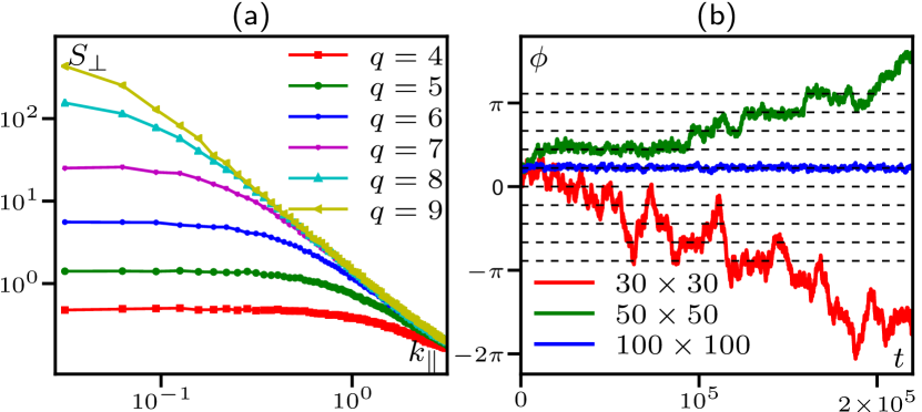
Figure 4: Ordered state in simulations of the PDE with noise ($\rho_{0}=5.5$, $\beta=4$, $D=1$, $v=1.8$) integrated with a space-time discretization $dx=1$ and $dt=0.05$. (a) Structure factor $S_{\perp}(\mathbf{k})=\langle m_{\perp}(\mathbf{k})m_{\perp}(\mathbf{-}\mathbf{k})\rangle$ vs $\mathbf{k}=(k_{\|},0)$ for various $q$ values (system size $200\times 200$). (b) Time series of the orientation of global order $\Phi$ showing a transition between unpinned and pinned dynamics as system size increases ($q=9$).

Let us now compare more precisely the behavior of Eqs. (4) to our microscopic clock model. To do that we complement Eq. (4b) with a white noise $\boldsymbol{\eta}(\mathbf{r},t)$ of random uniform orientation and Gaussian zero-mean unit-variance amplitude, and integrate the equations using a semi-spectral algorithm (linear terms are computed in Fourier space, nonlinear ones in real space) with Euler time stepping . The structure factor of $m_{\perp}$, shown in Fig. 4(a), is found to be qualitatively similar to that of Fig. 2. Moreover we also observe a pinning transition when $L$ is increased (Fig. 4(b)), as in Fig. 3 for the microscopic models.

All in all, at sufficiently large sizes, anisotropy is always relevant. This is markedly different from what happens in equilibrium where, for $q>4$, there is a range of temperature over which the anisotropy is irrelevant asymptotically, and one observes quasi-long-range order, as for a continuous spin. The argument used to derive a crossover length from the linearized hydrodynamic equation in Eq. (5) therefore fails in equilibrium. Indeed, there is no homogeneous ordered state to perturb from, only a quasi-ordered state with algebraically decaying correlations. This difference is essential, as is clear from looking at the scaling with system size of the energy $H_{q}=\int d^{2}\mathbf{r}\cos(q\theta(\mathbf{r}))$ due to the “clock potential”.

Let us then compare the scaling of $\langle H_{q}\rangle_{0}$ with the system size $L$, where the average is taken in the unperturbed system, without $H_{q}$, in equilibrium and in the active case. Of course, we do not actually have a Hamiltonian in our non-equilibrium model, but this argument should roughly capture the effect of the potential term in the equation of motion (4). Indeed, a more rigorous dynamical RG calculation that makes no use of analogies with equilibrium systems finds essentially the same result, as we will see below. In equilibrium, the unperturbed state can be described by the spin-wave Hamiltonian $H_{0}=\int d^{2}\mathbf{r}\frac{K}{2}[\nabla\theta(\mathbf{r})]^{2}$ with stiffness $K$. The perturbation is then evaluated as

$$\langle H_{q}\rangle_{0}\approx\int d^{2}\mathbf{r}\langle e^{iq\theta(\mathbf{r})}\rangle_{0}=\int d^{2}\mathbf{r}e^{-\frac{q^{2}}{2}G(\mathbf{0})}$$ (6)

where $G$ is the Green function of the Laplacian in infinite space. In Fourier space $\hat{G}(\mathbf{k})=\frac{T}{Kk^{2}}$, which, in 2D, gives $G(\mathbf{0})=T\log(L/\Lambda)/(2\pi K)$ for a system of size $L$, with $\Lambda$ a short distance cut-off. Inserting this into Eq. (6), one obtains

$$\langle H_{q}\rangle_{0}\sim L^{2-\frac{q^{2}T}{4\pi K}}.$$ (7)

From Eq. (7), we see that anisotropy is relevant when $L\to\infty$ whenever $T<T_{q}\equiv\frac{8\pi K}{q^{2}}$ and irrelevant otherwise. As a result, if $T_{1}<T_{BKT}=\frac{\pi K}{4}$ which happens for $q>q_{c}=4$, exactly, one observes a quasi-long range ordered phase where the anisotropy is irrelevant for $T_{1}<T<T_{\rm BKT}$, and a long-range ordered phase where the anisotropy is relevant for $T<T_{1}$.

In the active case, the ordered state of the unperturbed system is long-range ordered. Assuming that $\theta(\mathbf{r})$ shows Gaussian fluctuations with variance $\sigma^{2}$ around its mean value $\theta_{0}$ leads to $\langle e^{iq\theta(\mathbf{r})}\rangle_{0}=e^{-q^{2}\sigma^{2}/2}$. In turn, Eq. (6) becomes

$$\langle H_{q}\rangle_{0}^{\rm active}\approx\int\mathbf{d^{2}r}\langle e^{iq\theta(\mathbf{r})}\rangle_{0}=L^{2}e^{-q^{2}\sigma^{2}/2}$$ (8)

Anisotropy is thus always relevant when $L\gg L_{q}\equiv e^{q^{2}\sigma^{2}/4}$, so that $\langle H_{q}\rangle_{0}^{\rm active}\gg 1$. For $L\ll L_{q}$, on the contrary, anisotropy is exponentially suppressed by $q$ and Vicsek physics may be observed.

The argument above qualitatively explains the different responses to anisotropy observed in the active and passive cases, which are rooted in the different nature of the low temperature phases of their isotropic limits. In equilibrium, the scaling argument presented above has been made more rigorous using renormalization group calculations José et al. (1977); Elitzur et al. (1979). In the active case, the essential conclusions can also be shown to hold, following a dynamical renormalization group analysis Toner and Tu (1995); Toner (2012). This analysis shows that the length scale $L_{c\perp}$ beyond which the symmetry breaking field changes the physics obeys Solon et al.

$$L_{c\perp}(q,\sigma)=a\exp\left({q^{2}\sigma^{2}\over 2z}\right)\,.$$ (9)

where $a$ is a microscopic length and $z$ a dynamic exponent whose most recent numerical estimate is $z\simeq 1.33$ Mahault et al. (2019).

To summarize, we have shown that polar flocks are always susceptible to spatial anisotropy at sufficiently large system sizes. This is accompanied by a change of phenomenology compared to the isotropic Vicsek case: the direction of the order parameter is pinned, not wandering; structure factors at small $\mathbf{k}$ in the ordered phase are constant, not diverging; and one has macrophase separation at coexistence. However, this is felt only beyond a characteristic lengthscale that diverges for vanishingly small anisotropy. For the $q$-state active clock model considered here, the crossover can be understood from a hydrodynamic description where the discretization of the spin direction is accounted for by an effective potential. The crossover length is then shown to diverge exponentially with $q$, as observed in the microscopic model. The difference with the passive case can be accounted for using a scaling argument, that can be backed up by renormalization group analysis, which shows that the presence of long-range order is sufficient to render the anisotropy relevant asymptotically for any value of $q$ and $T$.

Our study is a first step in understanding spatial anisotropy in active matter. Its effect on other systems with a more complex phenomenology, such as active rods or active nematics, will deserve further investigations in the future. Finally, note that our choice of a lattice model was made for numerical efficiency. We checked that our results also hold in an off-lattice version of the model, but lack of impact of the lattice, which is anisotropic in nature, is almost surprising. How lattice anisotropy couples—or not—to the aligning dynamics would surely deserve a further study, possibly revealing a relevance at an even larger scale, out of reach of our numerical simulations.

Acknowledgements: We thank Mourtaza Kourbane-Houssene, for his early involvement in this work, as well as Benoît Mahault for a critical reading of the manuscript.

References

- Sanchez et al. (2012) T. Sanchez, D. T. Chen, S. J. DeCamp, M. Heymann, and Z. Dogic, Nature 491, 431 (2012).
- Li et al. (2019) H. Li, X.-q. Shi, M. Huang, X. Chen, M. Xiao, C. Liu, H. Chaté, and H. Zhang, Proceedings of the National Academy of Sciences 116, 777 (2019).
- Duclos et al. (2020) G. Duclos, R. Adkins, D. Banerjee, M. S. Peterson, M. Varghese, I. Kolvin, A. Baskaran, R. A. Pelcovits, T. R. Powers, and A. Baskaran, Science 367, 1120 (2020), publisher: American Association for the Advancement of Science.
- Wensink et al. (2012) H. H. Wensink, J. Dunkel, S. Heidenreich, K. Drescher, R. E. Goldstein, H. Löwen, and J. M. Yeomans, Proceedings of the National Academy of Sciences 109, 14308 (2012).
- Martinez et al. (2020) V. A. Martinez, E. Clément, J. Arlt, C. Douarche, A. Dawson, J. Schwarz-Linek, A. K. Creppy, V. Škultéty, A. N. Morozov, and H. Auradou, Proceedings of the National Academy of Sciences 117, 2326 (2020), publisher: National Acad Sciences.
- Buttinoni et al. (2013) I. Buttinoni, J. Bialké, F. Kümmel, H. Löwen, C. Bechinger, and T. Speck, Physical Review Letters 110, 238301 (2013).
- Geyer et al. (2019) D. Geyer, D. Martin, J. Tailleur, and D. Bartolo, Physical Review X 9, 031043 (2019), publisher: APS.
- Van Der Linden et al. (2019) M. N. Van Der Linden, L. C. Alexander, D. G. Aarts, and O. Dauchot, Physical Review Letters 123, 098001 (2019), publisher: APS.
- Cavagna et al. (2010) A. Cavagna, A. Cimarelli, I. Giardina, G. Parisi, R. Santagati, F. Stefanini, and M. Viale, Proceedings of the National Academy of Sciences 107, 11865 (2010).
- Bricard et al. (2013) A. Bricard, J.-B. Caussin, N. Desreumaux, O. Dauchot, and D. Bartolo, Nature 503, 95 (2013).
- Geyer et al. (2018) D. Geyer, A. Morin, and D. Bartolo, Nature materials 17, 789 (2018), publisher: Nature Publishing Group.
- Deseigne et al. (2010) J. Deseigne, O. Dauchot, and H. Chaté, Physical Review Letters 105, 098001 (2010).
- Kumar et al. (2014) N. Kumar, H. Soni, S. Ramaswamy, and A. Sood, Nature communications 5, 1 (2014), publisher: Nature Publishing Group.
- Chepizhko et al. (2013) O. Chepizhko, E. G. Altmann, and F. Peruani, Physical Review Letters 110, 238101 (2013), publisher: APS.
- Toner et al. (2018a) J. Toner, N. Guttenberg, and Y. Tu, Physical Review Letters 121, 248002 (2018a), publisher: APS.
- Toner et al. (2018b) J. Toner, N. Guttenberg, and Y. Tu, Physical Review E 98, 062604 (2018b), publisher: APS.
- Dor et al. (2019) Y. B. Dor, E. Woillez, Y. Kafri, M. Kardar, and A. P. Solon, Physical Review E 100, 052610 (2019), publisher: APS.
- Duan et al. (2021) Y. Duan, B. Mahault, Y.-q. Ma, X.-q. Shi, and H. Chaté, Physical Review Letters 126, 178001 (2021), publisher: APS.
- Ventejou et al. (2021) B. Ventejou, H. Chaté, R. Montagne, and X.-q. Shi, arXiv preprint arXiv:2107.14106 (2021).
- Ro et al. (2021) S. Ro, Y. Kafri, M. Kardar, and J. Tailleur, Physical Review Letters 126, 048003 (2021), publisher: APS.
- Dor et al. (2021) Y. B. Dor, S. Ro, Y. Kafri, M. Kardar, and J. Tailleur, arXiv preprint arXiv:2108.13409 (2021).
- Vicsek et al. (1995) T. Vicsek, A. Czirók, E. Ben-Jacob, I. Cohen, and O. Shochet, Physical Review Letters 75, 1226 (1995).
- Solon and Tailleur (2013) A. P. Solon and J. Tailleur, Physical Review Letters 111, 078101 (2013).
- Toner and Tu (1995) J. Toner and Y. Tu, Physical Review Letters 75, 4326 (1995).
- Toner and Tu (1998) J. Toner and Y. Tu, Physical Review E 58, 4828 (1998).
- Toner et al. (2005) J. Toner, Y. Tu, and S. Ramaswamy, Annals of Physics 318, 170 (2005).
- Toner (2012) J. Toner, Physical Review E 86, 031918 (2012).
- Mahault et al. (2019) B. Mahault, F. Ginelli, and H. Chaté, Physical Review Letters 123, 218001 (2019), publisher: APS.
- Solon et al. (2015a) A. P. Solon, H. Chaté, and J. Tailleur, Physical Review Letters 114, 068101 (2015a).
- Chaté et al. (2008) H. Chaté, F. Ginelli, G. Grégoire, and F. Raynaud, Physical Review E 77, 046113 (2008).
- Solon and Tailleur (2015) A. P. Solon and J. Tailleur, Physical Review E 92, 042119 (2015), publisher: APS.
- José et al. (1977) J. V. José, L. P. Kadanoff, S. Kirkpatrick, and D. R. Nelson, Physical Review B 16, 1217 (1977), publisher: APS.
- Elitzur et al. (1979) S. Elitzur, R. Pearson, and J. Shigemitsu, Physical Review D 19, 3698 (1979), publisher: APS.
- Tobochnik (1982) J. Tobochnik, Physical Review B 26, 6201 (1982), publisher: APS.
- Lapilli et al. (2006) C. M. Lapilli, P. Pfeifer, and C. Wexler, Physical Review Letters 96, 140603 (2006), publisher: APS.
- Li et al. (2020) Z.-Q. Li, L.-P. Yang, Z.-Y. Xie, H.-H. Tu, H.-J. Liao, and T. Xiang, Physical Review E 101, 060105 (2020), publisher: APS.
- Note (1) These rates are chosen such that if each site were isolated, the dynamics would satisfy detailed balance with steady-state probabilities and .
- (38) See supplementary information online.
- Note (2) For the AIM, it was shown that any amount of activity leads to the same phenomenology Solon and Tailleur (2015) and we have no reason to suspect a different behavior in our active clock model.
- Note (3) While this fit cannot be perfect, since the structure factor of the isotropic model is expected Toner and Tu (1995, 1998); Toner et al. (2005); Toner (2012) to scale like with neither nor equal to , both exponents are close enough to that this fit suffices to give a good estimate of .
- Note (4) Since we are interested in the homogeneous ordered phase, we do not need to complement the mean field equation with a density dependence of the coefficients, as required to observe the bands of the coexistence phase Solon et al. (2015b).
- (42) A. Solon, H. Chaté, J. Tailleur, and J. Toner, In preparation .
- Solon et al. (2015b) A. P. Solon, J.-B. Caussin, D. Bartolo, H. Chaté, and J. Tailleur, Physical Review E 92, 062111 (2015b).