Stochastic Continuous Submodular Maximization: Boosting via Non-oblivious Function

Abstract

In this paper, we revisit Stochastic Continuous Submodular Maximization in both offline and online settings, which can benefit wide applications in machine learning and operations research areas. We present a boosting framework covering gradient ascent and online gradient ascent. The fundamental ingredient of our methods is a novel non-oblivious function $F$ derived from a factor-revealing optimization problem, whose any stationary point provides a $(1-e^{-\gamma})$-approximation to the global maximum of the $\gamma$-weakly DR-submodular objective function $f\in C^{1,1}_{L}(\mathcal{X})$. Under the offline scenario, we propose a boosting gradient ascent method achieving $(1-e^{-\gamma}-\epsilon^{2})$-approximation after $O(1/\epsilon^{2})$ iterations, which improves the $(\frac{\gamma^{2}}{1+\gamma^{2}})$ approximation ratio of the classical gradient ascent algorithm. In the online setting, for the first time we consider the adversarial delays for stochastic gradient feedback, under which we propose a boosting online gradient algorithm with the same non-oblivious function $F$. Meanwhile, we verify that this boosting online algorithm achieves a regret of $O(\sqrt{D})$ against a $(1-e^{-\gamma})$-approximation to the best feasible solution in hindsight, where $D$ is the sum of delays of gradient feedback. To the best of our knowledge, this is the first result to obtain $O(\sqrt{T})$ regret against a $(1-e^{-\gamma})$-approximation with $O(1)$ gradient inquiry at each time step, when no delay exists, i.e., $D=T$. Finally, numerical experiments demonstrate the effectiveness of our boosting methods.

1 Introduction

Due to the relatively low computational complexity, first-order optimization methods are widely used in machine learning, operations research, and statistics communities. Especially for convex objectives, there is an enormous literature (Nesterov, 2013; Bertsekas, 2015) deriving the convergence rate of first-order methods. Recent studies have shown that first-order optimization methods could also achieve the global minimum for some special non-convex problems (Netrapalli et al., 2014; Arora et al., 2016; Ge et al., 2016; Du et al., 2019; Liu et al., 2020), although it is in general NP-hard to find the global minima of a non-convex objective function (Murty and Kabadi, 1987). Motivated by this, some recent work focused on the structures and conditions under which non-convex optimization is tractable (Bian et al., 2017; Hazan et al., 2016a). In this paper, we investigate the stochastic $\gamma$-weakly continuous submodular maximization problem where an unbiased gradient oracle is available under both offline and online scenarios.

Continuous DR-Submodular Maximization has drawn much attention recently due to that it admits efficient approximate maximization routines. For instance, under the offline deterministic setting, Bian et al. (2017, 2020) proposed the vanilla Frank-Wolfe method and its variant achieving $1/2$ and $(1-1/e)$ approximations, respectively. When the stochastic estimates of the gradient is available, Mokhtari et al. (2018) and Hassani et al. (2020) proposed some improved variants of the Frank-Wolfe algorithm, equipped with variance reduction techniques. In (Hassani et al., 2020), assuming the Lipschitz continuity of stochastic Hessian, a $[(1-1/e)OPT-\varepsilon]$ solution is achieved using $O(1/\varepsilon^{2})$ stochastic gradient. Such a result provides the tightest approximation as well as the optimal stochastic first-order oracle complexity.

However, when generalizing Frank-Wolfe methods to the online setting, some other tricks should be involved, which makes the algorithm design more complicated. For example, Chen et al. (2018b) and Zhang et al. (2019) took the idea of meta actions (Streeter and Golovin, 2008) and blocking procedure to propose online Frank-Wolfe algorithms. Moreover, in these aforementioned studies, the environment/adversary reveals the reward and stochastic first-order information immediately after the action is chosen by the learner/algorithm. In practice, the assumption of immediate feedback might be too restrictive. The feedback delays widely exist in many real-world applications, e.g., online advertising (Mehta et al., 2007), influence maximization problem (Chen et al., 2012; Yang et al., 2016).

To tackle these issues, instead of Frank-Wolfe, we adopt Gradient Ascent and aim to propose a uniform algorithmic framework for both offline and online Stochastic Continuous Submodular Maximization. To make the online setting more realistic, we also consider adversarial feedback delays (Quanrud and Khashabi, 2015). Note that our online setting degenerates to the standard online setting if no delay exists. One big challenge in front of us is that the stationary points of a $\gamma$-weakly submodular function $f$ only provide a limited $(\frac{\gamma^{2}}{1+\gamma^{2}})$-approximation to the global maximum Hassani et al. (2017). As a result, we need to boost stochastic gradient ascent and its online counterpart (Hassani et al., 2017) as they only attain a $(\frac{\gamma^{2}}{1+\gamma^{2}})$-approximation. To tackle this challenge, we hope to devise an auxiliary function whose stationary points provide a better approximation guarantee than those of $f$ itself. Motivated by (Feldman et al., 2011; Filmus and Ward, 2012, 2014; Harshaw et al., 2019; Feldman, 2021; Mitra et al., 2021), we first consider a family of auxiliary functions whose gradient at point $\boldsymbol{x}$ allocates different weight to the gradient $\nabla f(z*\boldsymbol{x})$ where $z\in[0,1]$. By solving a factor-revealing optimization problem, we select the optimal auxiliary function $F$ whose stationary points provide a tight $(1-e^{-\gamma})$-approximation to the global maximum of $f$. Then, based on this optimal auxiliary function $F$, we propose a simple first-order framework that makes it possible to boost the performance of classical gradient ascent algorithm converging to stationary points.

Based on this boosting framework, we present a boosting gradient ascent and a boosting online gradient ascent to improve the approximation guarantees of vanilla gradient ascent and its online counterpart. To be specific, we make the following contributions:

1. We develop a uniform boosting framework, including gradient ascent and online gradient ascent methods. The essential element behind our framework is an optimal auxiliary function $F$ derived from a factor-revealing optimization problem for each $\gamma$-weakly DR-submodular function $f$. The stationary points of $F$ provide a $(1-e^{-\gamma})$-approximation guarantee to the global maximum of $f$. This approximation is better than the $(\frac{\gamma^{2}}{1+\gamma^{2}})$-approximation provided by stationary points of $f$ itself.

2. With this non-oblivious function $F$, under the offline setting, we propose the boosting gradient ascent method achieving a $(1-e^{-\gamma}-\epsilon^{2})$-approximation after $O(1/\epsilon^{2})$ iterations, which improves the $(\frac{\gamma^{2}}{1+\gamma^{2}})$-approximation of the classical projected gradient ascent algorithm and weakens the assumption of high order smoothness on the objective functions (Hassani et al., 2020).

3. Next, we consider an online submodular maximization setting with adversarial feedback delays. When an unbiased stochastic gradients estimation is available, we propose an online boosting gradient ascent algorithm that theoretically achieves the optimal $(1-e^{-\gamma})$-regret of $O(\sqrt{D})$ with one gradient evaluation for each $f_{t}$, where $D=\sum_{t=1}^{T}d_{t}$ and $d_{t}$ is a positive integer delay for round $t$. To the best of our knowledge, our work is the first to investigate the adversarial delays in online submodular maximization problems. Moreover, when $D=T$ for the standard no-delay setting, our proposed online boosting gradient ascent algorithm, requiring only $O(1)$ stochastic gradient estimate at each round, yields the first result to achieve $(1-e^{-\gamma})$-approximation with $O(\sqrt{T})$ regret.

4. Finally, we empirically evaluate our proposed boosting methods using the special example of (Hassani et al., 2017) and the simulated non-convex/non-concave quadratic programming. Our algorithms have superior performance in the experiments.

Table 1: Comparison of convergence guarantees for continuous DR-submodular function maximization, where the functions are monotone. Except for Bian et al. (2017) which needs the constraint set to be convex and down-closed, other methods here need the constraint set $\mathcal{C}$ to be convex. Note that ’det.’ and ’sto.’ represent the deterministic and stochastic setting, respectively. ’Hess Lip’ means whether the Hessian of functions needs to be Lipschitz continuous, ’OPT’ is the function value at the global optimum, ’Complexity’ is the gradient oracle complexity. For simplicity, we set $\gamma=1$ for our results which reduces to the standard monotone DR-submodular setting.

Method	Setting	Hess Lip	Utility	Complexity
Submodular FW (Bian et al., 2017)	det.	No	$(1-1/e)\rm{OPT}-\epsilon$	$O(1/\epsilon)$
SGA (Hassani et al., 2017)	sto.	No	$(1/2)\rm{OPT}-\epsilon$	$O(1/\epsilon^{2})$
Classical FW (Bian et al., 2020)	det.	No	$(1/2)\rm{OPT}-\epsilon$	$O(1/\epsilon^{2})$
SCG (Mokhtari et al., 2018)	sto.	No	$(1-1/e)\rm{OPT}-\epsilon$	$O(1/\epsilon^{3})$
SCG++ (Hassani et al., 2020)	sto.	Yes	$(1-1/e)\rm{OPT}-\epsilon$	$O(1/\epsilon^{2})$
Non-Oblivious FW (Mitra et al., 2021)	det.	No	$(1-1/e-\epsilon)\rm{OPT}-\epsilon$	$O(1/\epsilon^{3})$
Boosting GA (This paper)	sto.	No	$(1-1/e-\epsilon^{2})\rm{OPT}-\epsilon$	$O(1/\epsilon^{2})$

1.1 Related Work

Submodular Set Functions: Submodular set functions originate from combinatorial optimization problems (Nemhauser et al., 1978; Fisher et al., 1978; Fujishige, 2005), which could be either exactly minimized via Lovász extension (Lovász, 1983) or approximately maximized via multilinear extension (Chekuri et al., 2014). Submodular set functions find numerous applications in machine learning and other related areas, including viral marketing (Kempe et al., 2003), document summarization (Lin and Bilmes, 2011), network monitoring (Leskovec et al., 2007), and variable selection (Das and Kempe, 2011; Elenberg et al., 2018).

Continuous Submodular Maximization: Submodularity can be naturally extended to continuous domains. In deterministic setting, Bian et al. (2017) first proposed a variant of Frank-Wolfe (Submodular FW) for continuous DR-submodular maximization problem with $(1-1/e)$-approximation guarantee after $O(1/\epsilon)$ iterations. As for the stochastic setting, Hassani et al. (2017) proved that the stochastic gradient ascent (SGA) guarantees a $(1/2)$-approximation after $O(1/\epsilon^{2})$ iterations. Then, Mokhtari et al. (2018) proposed the stochastic continuous greedy algorithm (SCG), which achieves a $(1-1/e)$-approximation after $O(1/\epsilon^{3})$ iterations. Moreover, by assuming the Hessian of objective is Lipschitz continuous, Hassani et al. (2020) proposed the stochastic continuous greedy++ algorithm (SCG++), which guarantees a $(1-1/e)$-approximation after $O(1/\epsilon^{2})$ iterations.

Online Continuous Submodular Maximization: Chen et al. (2018b) first investigated the online (stochastic) gradient ascent (OGA) with a $(1/2)$-regret of $O(\sqrt{T})$. Then, inspired by the meta actions (Streeter and Golovin, 2008), Chen et al. (2018b) also proposed the Meta-Frank-Wolfe algorithm with a $(1-1/e)$-regret bound of $O(\sqrt{T})$ under the deterministic setting. Assuming that an unbiased estimation of the gradient is available, Chen et al. (2018a) proposed a variant of the Meta-Frank-Wolfe algorithm (Meta-FW-VR) having a $(1-1/e)$-regret bound of $O(T^{1/2})$ and requiring $O(T^{3/2})$ stochastic gradient queries for each function. Then, in order to reduce the number of gradients evaluation, Zhang et al. (2019) presented the Mono-Frank-Wolfe taking the blocking procedure, which achieves a $(1-1/e)$-regret bound of $O(T^{4/5})$ with only one stochastic gradient evaluation in each round.

Table 2: Comparison of regrets for stochastic online continuous DR-submodular function maximization with full-information feedback, where the functions are monotone and constraint set $\mathcal{C}$ is convex. Note that ’# Grad. Evaluations ’ means the number of stochastic gradient evaluations at each round, ’Ratio’ means approximation ratio, and ’Delay’ indicates whether the adversarial delayed feedback is considered. For simplicity, we set $\gamma=1$ for our results which reduces to the standard monotone DR-submodular setting, and $D=T$ which means no delay exists.

Method	# Grad. Evaluations	Ratio	Regret	Delay
OGA (Chen et al., 2018b)	$O(1)$	$1/2$	$O(\sqrt{T})$	No
Meta-FW-VR (Chen et al., 2018a)	$T^{3/2}$	$1-1/e$	$O(\sqrt{T})$	No
Mono-FW (Zhang et al., 2019)	$O(1)$	$1-1/e$	$O(T^{4/5})$	No
Boosting OGA (This paper)	$O(1)$	$1-1/e$	$O(\sqrt{T})$	Yes

Non-Oblivious Search: In many cases, classical local search, e.g., the greedy method, may return a solution with a poor approximation ratio to the global maximum. To avoid this issue, Khanna et al. (1998) and Alimonti (1994) first proposed a technique named Non-Oblivious Search that leverages an auxiliary function to guide the search. After carefully choosing the auxiliary function, the new solution generated by the non-oblivious search, may have a better performance than the previous solution found by the classical local search. Inspired by this idea, for the maximum coverage problem over a matroid, Filmus and Ward (2012) proposed a $(1-1/e)$-approximation algorithm via a non-oblivious set function allocating extra weights to the solutions that cover some element more than once, which efficiently improves the traditional $(1/2)$-approximation greedy method. After that, Filmus and Ward (2014) extended this idea to improve the $(1/2)$-approximation greedy method for the general submodular set maximization problem over a matroid. Recently, for the continuous submodular maximization problem with concave regularization, a variant of Frank-Wolfe algorithm (Non-Oblivious FW) based on a special auxiliary function was proposed for boosting the approximation ratio of the submodular part from $1/2$ to $(1-1/e)$ in (Mitra et al., 2021). Compared to the proposed algorithm in this paper, i) The Non-Oblivious Frank-Wolfe method needs $O(1/\epsilon)$ gradient evaluations at each round under the deterministic setting, while our method only needs $O(1)$ evaluations per iteration under the stochastic setting; ii) The Non-Oblivious Frank-Wolfe method is designed only for the deterministic setting, while we present a uniform boosting framework covering the stochastic gradient ascent in both offline and online settings.

We present comparisons between this work and previous studies in Table 1 and Table 2 for offline and online settings, respectively.

2 Preliminaries

In this section, we define some concepts and notations that we will use throughout the paper.

2.1 Continuous Submodularity

Continuous Submodular Functions: A function $f:\mathcal{X}\rightarrow\mathbb{R}_{+}$ is a continuous submodular function if for any $\boldsymbol{x},\boldsymbol{y}\in\mathcal{X}$,

$$f(\boldsymbol{x})+f(\boldsymbol{y})\geq f(\boldsymbol{x}\land\boldsymbol{y})+f(\boldsymbol{x}\lor\boldsymbol{y}).$$

Here, $\boldsymbol{x}\land\boldsymbol{y}=\min(\boldsymbol{x},\boldsymbol{y})$ and $\boldsymbol{x}\lor\boldsymbol{y}=\max(\boldsymbol{x},\boldsymbol{y})$ are component-wise minimum and component-wise maximum, respectively. $\mathcal{X}=\prod_{i=1}^{n}\mathcal{X}_{i}$ where each $\mathcal{X}_{i}$ is a compact interval in $\mathbb{R}_{+}$. Without loss of generality, we assume $\mathcal{X}_{i}=[0,a_{i}]$. If $f$ is twice differentiable, the continuous submodularity is equivalent to

$$\forall i\neq j,\forall\boldsymbol{x}\in\mathcal{X},\frac{\partial^{2}f(\boldsymbol{x})}{\partial x_{i}\partial x_{j}}\leq 0.$$

Moreover, $f$ is monotone if $f(\boldsymbol{x})\geq f(\boldsymbol{y})$ when $\boldsymbol{x}\geq\boldsymbol{y}$.

DR-Submodularity: A continuous submodular function $f$ is DR-submodular if

$$f(\boldsymbol{x}+z\boldsymbol{e}_{i})-f(\boldsymbol{x})\leq f(\boldsymbol{y}+z\boldsymbol{e}_{i})-f(\boldsymbol{y}),$$

where $\boldsymbol{e}_{i}$ is the $i$-th basic vector, $\boldsymbol{x}\geq\boldsymbol{y}$ and $z\in\mathbb{R}_{+}$ such that $\boldsymbol{x}+z\boldsymbol{e}_{i},\boldsymbol{y}+z\boldsymbol{e}_{i}\in\mathcal{X}$. When the DR-submodular function $f$ is differentiable, we have $\nabla f(\boldsymbol{x})\leq\nabla f(\boldsymbol{y})$ if $\boldsymbol{x}\geq\boldsymbol{y}$ (Bian et al., 2020). When $f$ is twice differentiable, the DR-submodularity is also equivalent to

$$\forall i,j\in[n],\forall\boldsymbol{x}\in\mathcal{X},\frac{\partial^{2}f(\boldsymbol{x})}{\partial x_{i}\partial x_{j}}\leq 0.$$

Furthermore, we call a function $f$ weakly DR-submodular with parameter $\gamma$, if

$$\gamma=\inf_{\boldsymbol{x}\leq\boldsymbol{y}}\inf_{i\in[n]}\frac{[\nabla f(\boldsymbol{x})]_{i}}{[\nabla f(\boldsymbol{y})]_{i}}.$$

Note that $\gamma=1$ indicates a differentiable and monotone DR-submodular function.

2.2 Notations and Concepts

Norm: $\left\|\cdot\right\|$ is the $\ell_{2}$ norm in Euclidean space.

Radius and Diameter: For any bounded domain $\mathcal{C}\in\mathcal{X}$, the radius $r(\mathcal{C})=\max_{\boldsymbol{x}\in\mathcal{C}}\left\|\boldsymbol{x}\right\|$ and the diameter $\mathrm{diam}(\mathcal{C})=\max_{\boldsymbol{x},\boldsymbol{y}\in\mathcal{C}}\left\|\boldsymbol{x}-\boldsymbol{y}\right\|$.

Projection: We define the projection to the domain $\mathcal{C}$ as $\mathcal{P}_{\mathcal{C}}(\boldsymbol{x})=\arg\min_{\boldsymbol{z}\in\mathcal{C}}\left\|\boldsymbol{x}-\boldsymbol{z}\right\|$.

Smoothness: A differentiable function $f$ is called $L$-$smooth$ if for any $\boldsymbol{x},\boldsymbol{y}\in\mathcal{X}$,

$$\left\|\nabla f(\boldsymbol{x})-\nabla f(\boldsymbol{y})\right\|\leq L\left\|\boldsymbol{x}-\boldsymbol{y}\right\|.$$

$\alpha$-Regret: Finally, we recall the $\alpha$-regret in (Chen et al., 2018b). For a $T$-$round$ game, after the algorithm $\mathcal{A}$ choose an action $\boldsymbol{x}_{t}\in\mathcal{X}$ in each round, the adversary reveals the utility function $f_{t}$. The objective of the algorithm $\mathcal{A}$ is to minimize the gap between the accumulative reward and that of the best fixed policy in hindsight with scale parameter $\alpha$, i.e.,

$$\mathcal{R}_{\alpha}(\mathcal{A},T)=\alpha\max_{\boldsymbol{x}\in\mathcal{X}}\sum_{t=1}^{T}f_{t}(\boldsymbol{x})-\sum_{t=1}^{T}f_{t}(\boldsymbol{x}_{t}).$$

3 Derivation of the Non-oblivious Function

In this section, we present in detail how to derive our non-oblivious function, which plays an important role in our boosting framework. To begin, we recall the definition of stationary points.

Definition 1

A point $\boldsymbol{x}\in\mathcal{C}$ is called a stationary point for function $f:\mathcal{X}\rightarrow\mathbb{R}_{+}$ over the domain $\mathcal{C}\subseteq\mathcal{X}$ if

$$\max_{\boldsymbol{y}\in\mathcal{C}}\langle\nabla f(\boldsymbol{x}),\boldsymbol{y}-\boldsymbol{x}\rangle\leq 0.$$

We make the following assumption throughout this paper.

Assumption 1

1. The $f:\mathcal{X}\rightarrow\mathbb{R}_{+}$ is a monotone, differentiable, weakly DR-submodular function with parameter $\gamma$. So is each $f_{t}$ in the online settings.

2. We also assume the knowledge of parameter $\gamma$.

3. Without loss of generality, $f(\boldsymbol{0})=0$. Also, in online settings, $f_{t}(\boldsymbol{0})=0$ for $t=1,2,\dots,T$.

With this assumption, we have the following result.

Lemma 1 (Proof in Section A.1)

Under Assumption 1, for any stationary point $\boldsymbol{x}\in\mathcal{C}$ of $f$, we have

$$f(\boldsymbol{x})\geq\frac{\gamma^{2}}{\gamma^{2}+1}\max_{\boldsymbol{y}\in\mathcal{C}}f(\boldsymbol{y}).$$ (1)

Remark 1

Lemma 1 implies any stationary point of a $\gamma$-weakly DR-submodular function $f$ provides a $(\frac{\gamma^{2}}{1+\gamma^{2}})$-approximation to the global maximum. As we know, projected gradient ascent method (Hassani et al., 2017) with small step size usually converges to a stationary point of $f$, resulting in a $(\frac{\gamma^{2}}{1+\gamma^{2}})$ approximation guarantee.

In order to boost these classical algorithms, a natural idea is to design some auxiliary functions whose stationary points achieve better approximation to the global maximum of the problem $\max_{\boldsymbol{x}\in\mathcal{C}}f(\boldsymbol{x})$. That is, we want to find $F:\mathcal{X}\rightarrow\mathbb{R}_{+}$ based on $f$ such that $\langle\boldsymbol{y}-\boldsymbol{x},\nabla F(\boldsymbol{x})\rangle\geq\beta_{1}f(\boldsymbol{y})-\beta_{2}f(\boldsymbol{x})$, where $\beta_{1}/\beta_{2}\geq\frac{\gamma^{2}}{1+\gamma^{2}}$.

Motivated by (Feldman et al., 2011; Filmus and Ward, 2012, 2014; Harshaw et al., 2019; Feldman, 2021; Mitra et al., 2021), we consider the function $F(\boldsymbol{x}):\mathcal{X}\rightarrow\mathbb{R}_{+}$ whose gradient at point $\boldsymbol{x}$ allocates different weights to the gradient $\nabla f(z*\boldsymbol{x})$, i.e., $\nabla F(\boldsymbol{x})=\int_{0}^{1}w(z)\nabla f(z*\boldsymbol{x})\mathrm{d}z$, assuming that $\nabla f(z*\boldsymbol{x})$ is Lebesgue integrable w.r.t. $z\in[0,1]$, the weight function $w(z)\in C^{1}[0,1]$, and $w(z)\geq 0$. Then, we investigate a property of $\langle\boldsymbol{y}-\boldsymbol{x},\nabla F(\boldsymbol{x})\rangle$ in the following lemma.

Lemma 2 (Proof in Section A.2)

For all $\boldsymbol{x},\boldsymbol{y}\in\mathcal{X}$, we have

$$\langle\boldsymbol{y}-\boldsymbol{x},\nabla F(\boldsymbol{x})\rangle\geq\left(\gamma\int_{0}^{1}w(z)dz\right)\left(f(\boldsymbol{y})-\theta(w)f(\boldsymbol{x})\right),$$

where $\theta(w)=\max_{f,\boldsymbol{x}}\theta(w,f,\boldsymbol{x})$, $\theta(w,f,\boldsymbol{x})=\frac{w(1)+\int^{1}_{0}(\gamma w(z)-w^{\prime}(z))\frac{f(z*\boldsymbol{x})}{f(\boldsymbol{x})}\mathrm{d}z}{\gamma\int_{0}^{1}w(z)\mathrm{d}z}$ and $f(\boldsymbol{x})>0$.

To improve the approximation ratio, we consider the following factor-revealing optimization problem:

$$\min_{w}\theta(w)=\min_{w} \max_{f,\boldsymbol{x}}\frac{w(1)+\int^{1}_{0}(\gamma w(z)-w^{\prime}(z))\frac{f(z*\boldsymbol{x})}{f(\boldsymbol{x})}\mathrm{d}z}{\gamma\int_{0}^{1}w(z)\mathrm{d}z}$$ (2)

$$\rm{s.t.} w(z)\geq 0,$$

$$w(z)\in C^{1}[0,1],$$

$$f(\boldsymbol{x})>0,$$

$$\nabla f(\boldsymbol{x}_{1})\geq\gamma\nabla f(\boldsymbol{y}_{1})\geq\boldsymbol{0},\forall\boldsymbol{x}_{1}\leq\boldsymbol{y}_{1}\in\mathcal{X}.$$

At first glance, problem (2) looks challenging to solve. Fortunately, we could directly find the optimal solution, which is provided in the following theorem.

Theorem 1 (Proof in the Section A.3)

For problem (2), we have $\hat{w}(z)=e^{\gamma(z-1)}\in\arg\min_{w}\theta(w)$ and $\min_{w}\max_{f,\boldsymbol{x}}\theta(w,f,\boldsymbol{x})=\frac{1}{1-e^{-\gamma}}$.

In the following sections, we consider this optimal auxiliary function $F$ with $\nabla F(\boldsymbol{x})=\int_{0}^{1}\hat{w}(z)\nabla f(z*\boldsymbol{x})\mathrm{d}z$, and $\hat{w}(z)=e^{\gamma(z-1)}$. According to the definition of $\theta(w,f,\boldsymbol{x})$ in Lemma 2, we could derive that $\theta(\hat{w},f,\boldsymbol{x})=\hat{w}(1)/(\gamma\int_{0}^{1}\hat{w}(z)\mathrm{d}z)=1/(1-e^{-\gamma})$ such that $\theta(\hat{w})=1/(1-e^{-\gamma})$. Thus, we have $\langle\boldsymbol{y}-\boldsymbol{x},\nabla F(\boldsymbol{x})\rangle\geq(1-e^{-\gamma})f(\boldsymbol{y})-f(\boldsymbol{x})$ which implies that any stationary point of $F$ provides a better $(1-e^{-\gamma})$-approximation solution to the problem $\max_{\boldsymbol{x}\in\mathcal{C}}f(\boldsymbol{x})$, in contrast with the stationary points of $f$ itself.

Next, we investigate some properties of this optimal auxiliary function $F(\boldsymbol{x})$. Following the same terminology in (Filmus and Ward, 2012, 2014; Mitra et al., 2021), we also call this $F$ the non-oblivious function.

3.1 Properties about the Non-Oblivious Function

Without loss of generality, in this subsection, we assume $f$ is $L$-smooth with respect to the norm $\left\|\boldsymbol{x}\right\|$, i.e., $\left\|\nabla f(\boldsymbol{x})-\nabla f(\boldsymbol{y})\right\|\leq L\left\|\boldsymbol{x}-\boldsymbol{y}\right\|$. Then, we establish some key properties about the boundness and smoothness of the non-oblivious function $F(\boldsymbol{x})$ in the following theorem.

Theorem 2 (Proof in Section A.4)

If $f$ is $L$-smooth, and Assumption 1 holds, we have

1. $f(\boldsymbol{x})\geq(1-e^{-\gamma})\max_{\boldsymbol{y}\in\mathcal{C}}f(\boldsymbol{y})$, where $\boldsymbol{x}$ is a stationary point for non-oblivious function $F$ over the domain $\mathcal{C}$.

2. $F(\boldsymbol{x})=\int_{0}^{1}\frac{e^{\gamma(z-1)}}{z}f(z*\boldsymbol{x})dz$ and $F(\boldsymbol{x})\leq(1+\ln(\tau))(f(\boldsymbol{x})+c)$ for any positive $c\leq Lr^{2}(\mathcal{X})$, where $\tau=\max(\frac{1}{\gamma},\frac{Lr^{2}(\mathcal{X})}{c})$.

3. $F$ is $L_{\gamma}$-smooth where $L_{\gamma}=L\frac{\gamma+e^{-\gamma}-1}{\gamma^{2}}$.

Remark 2

Theorem 2.(i) demonstrates that any stationary point of the non-oblivious function $F$ can attain $(1-e^{-\gamma})$-approximation of the global maximum of $f$, which is better than the $(\frac{\gamma^{2}}{1+\gamma^{2}})$-approximation ratio of the stationary points of $f$ itself provided in Lemma 1. Moreover, this result sheds light on the possibility of utilizing $F$ to obtain a better approximation than classical gradient ascent method, which motivates our boosting methods in the following section.

We also investigate how to estimate $\nabla F(\boldsymbol{x})$ with an unbiased stochastic oracle $\widetilde{\nabla}f(\boldsymbol{x})$, i.e., $\mathbb{E}(\widetilde{\nabla}f(\boldsymbol{x})|\boldsymbol{x})=\nabla f(\boldsymbol{x})$. We first introduce a new random variable $\mathbf{Z}$ where Pr$(\mathbf{Z}\leq z)=\int_{0}^{z}\frac{\gamma e^{\gamma(u-1)}}{1-e^{-\gamma}}I(u\in[0,1])\mathrm{d}u$ where $I$ is the indicator function. When the number $z$ is sampled from r.v. $\mathbf{Z}$, we consider $\frac{1-e^{-\gamma}}{\gamma}\widetilde{\nabla}f(z*\boldsymbol{x})$ as an estimator of $\nabla F(\boldsymbol{x})$ with statistical properties given in the following proposition.

Proposition 1 (Proof in Section A.5)

1. If $z$ is sampled from r.v. $\mathbf{Z}$ and $\mathbb{E}(\widetilde{\nabla}f(\boldsymbol{x})|\boldsymbol{x})=\nabla f(\boldsymbol{x})$, we have

   $$\mathbb{E}\left(\left.\frac{1-e^{-\gamma}}{\gamma}\widetilde{\nabla}f(z*\boldsymbol{x})\right|\boldsymbol{x}\right)=\nabla F(\boldsymbol{x}).$$

2. If $z$ is sampled from r.v. $\mathbf{Z}$, $\mathbb{E}(\widetilde{\nabla}f(\boldsymbol{x})|\boldsymbol{x})=\nabla f(\boldsymbol{x})$, and $\mathbb{E}(\|\widetilde{\nabla}f(\boldsymbol{x})-\nabla f(\boldsymbol{x})\|^{2}|\boldsymbol{x})\leq\sigma^{2}$, we have

   $$\mathbb{E}\left(\bigg{\|}\frac{1-e^{-\gamma}}{\gamma}\widetilde{\nabla}f(z*\boldsymbol{x})-\nabla F(\boldsymbol{x})\bigg{\|}^{2}\bigg{|}\boldsymbol{x}\right)\leq\sigma^{2}_{\gamma},$$

   where $\sigma^{2}_{\gamma}=2\frac{(1-e^{-\gamma})^{2}\sigma^{2}}{\gamma^{2}}+\frac{2L^{2}r^{2}(\mathcal{X})(1-e^{-2\gamma})}{3\gamma}$.

Remark 3

Proposition 1 indicates that $\frac{1-e^{-\gamma}}{\gamma}\widetilde{\nabla}f(z*\boldsymbol{x})$ is an unbiased estimator of $\nabla F(\boldsymbol{x})$ with a bounded variance.

4 Boosting Framework

Algorithm 1 Meta Boosting Protocol

1:  Initialize: any $\boldsymbol{x}_{1}\in\mathcal{X}$.

2:  for $t\in[T]$ do

3:     Sample $z_{t}$ from $\mathbf{Z}$ where $\mathrm{P}(\mathbf{Z}\leq z)=\int_{0}^{z}\frac{\gamma e^{\gamma(u-1)}}{1-e^{-\gamma}}I(u\in[0,1])\mathrm{d}u$.

4:     Compute $\widetilde{\nabla}F(\boldsymbol{x}_{t})=\frac{1-e^{-\gamma}}{\gamma}\widetilde{\nabla}f(z_{t}*\boldsymbol{x}_{t})$

5:     Update $\boldsymbol{x}_{t+1}=\mathcal{A}(\widetilde{\nabla}F(\boldsymbol{x}_{t}),\boldsymbol{x}_{t})$                               {$\triangleright$$\mathcal{A}$ to be designed.}

6:  end for

7:  Option I (Offline setting): Return $\boldsymbol{x}_{l}$ chosen from $\{\boldsymbol{x}_{t}\}_{t\in[T]}$ with a probability.

8:  Option II (Online setting): Return $\boldsymbol{x}_{t}$ at each round $t\in[T]$.

Up to this point, we present a boosting framework that covers both gradient ascent and online gradient ascent methods. We first present a Meta boosting protocol in Algorithm 1, highlighting the key features of the proposed algorithms. We then present several variants of the Meta protocol by employing different basic algorithms $\mathcal{A}$.

As shown in Algorithm 1, the core idea is to leverage the stochastic gradient $\widetilde{\nabla}F(\boldsymbol{x}_{t})$ of the non-oblivious function $F$, instead of the stochastic gradient $\widetilde{\nabla}f(\boldsymbol{x}_{t})$ of the original weakly DR-submodular function $f$. Note that $\widetilde{\nabla}F(\boldsymbol{x}_{t})$ is generated by the sampling method in Proposition 1 (line 3-4 of Algorithm 1).

4.1 Boosting Gradient Ascent

Algorithm 2 Boosting Gradient Ascent

Input: $T$, $\eta_{t}$, $c>0$, $\gamma$, $L$, $r(\mathcal{X})$
  Output: $\boldsymbol{x}_{l}$

1:  Set $\triangle_{t}=1$ when $t<T$ and $\triangle_{T}=1+\ln(\tau)$ where $\tau=\max(\frac{1}{\gamma},\frac{r^{2}(\mathcal{X})L}{c})$.

2:  Set $\triangle=\sum_{t=1}^{T}\triangle_{t}$

3:  Initialize any $\boldsymbol{x}_{1}\in\mathcal{X}$.

4:  for $t\in[T]$ do

5:     Compute $\widetilde{\nabla}F(\boldsymbol{x}_{t})$ according to Algorithm 1

6:     Set $\boldsymbol{y}_{t+1}=\boldsymbol{x}_{t}+\eta_{t}\widetilde{\nabla}F(\boldsymbol{x}_{t})$

7:     $\boldsymbol{x}_{t+1}=\arg\min_{\boldsymbol{z}\in\mathcal{C}}\left\|\boldsymbol{z}-\boldsymbol{y}_{t+1}\right\|$

8:  end for

9:  Choose a number $l\in[T]$ with the distribution $\mathrm{P}(l=t)$=$\frac{\triangle_{t}}{\triangle}$

In this subsection, we propose a boosting gradient ascent method under the offline scenario for the stochastic submodular maximization problem. In particular, we employ the classical stochastic projected gradient ascent method in the Meta boosting protocol and describe the boosting gradient ascent method in Algorithm 2.

As demonstrated in Algorithm 2, in each iteration, after calculating $\widetilde{\nabla}F(\boldsymbol{x})$, we make the standard projected gradient step to update $\boldsymbol{x}$. Finally, we return $\boldsymbol{x}_{l}$ chosen from $\{\boldsymbol{x}_{t}\}_{t\in[T]}$ with the given distribution.

With the previous outcomes, we establish the convergence result for Algorithm 2.

Theorem 3 (Proof in Section B)

Assume $\mathcal{C}\in\mathcal{X}$ is a bounded convex set and $f$ is $L$-$smooth$, and the gradient oracle $\widetilde{\nabla}f(\boldsymbol{x})$ is unbiased with $\mathbb{E}(\|\widetilde{\nabla}f(\boldsymbol{x})-\nabla f(\boldsymbol{x})\|^{2}|\boldsymbol{x})\leq\sigma^{2}$. Let $\eta_{t}=\frac{1}{\frac{\sigma_{\gamma}\sqrt{t}}{\mathrm{diam}(\mathcal{C})}+L_{\gamma}}$ and $c=O(1)$ in Algorithm 2, then we have

$$\mathbb{E}(f(\boldsymbol{x}_{l}))\geq\bigg{(}1-e^{-\gamma}-O\Big{(}\dfrac{1}{T}\Big{)}\bigg{)}OPT-O\Big{(}\dfrac{1}{\sqrt{T}}\Big{)},$$

where $OPT=\max_{\boldsymbol{x}\in\mathcal{C}}f(\boldsymbol{x})$.

Remark 4

Theorem 3 shows that after $O(1/\epsilon^{2})$ iterations, the boosting stochastic gradient ascent achieves $(1-1/e-\epsilon^{2})OPT-\epsilon$, which efficiently improves the $(1/2)$-approximation guarantee of classical stochastic gradient ascent (Hassani et al., 2017) for continuous DR-submodular maximization. Moreover, we highlight that the overall gradient complexity is $O(1/\epsilon^{2})$ which is optimal (Hassani et al., 2020) under the stochastic setting.

4.2 Online Boosting Delayed Gradient Ascent

In this section, we consider the online setting with delayed feedback. To begin, recall the process of classical online optimization. In round $t$, after picking an action $\boldsymbol{x}_{t}\in\mathcal{C}$, the environment (adversary) gives a utility $f_{t}(\boldsymbol{x}_{t})$ and permits the access to the stochastic gradient of $f_{t}$. The objective is to minimize the $\alpha$-regret for $T$ planned rounds. Then, we turn to the (adversarial) feedback delays phenomenon (Quanrud and Khashabi, 2015) in our online stochastic submodular maximization problem. That is, instead of the prompt feedback, the information about the stochastic gradient of $f_{t}$ could be delivered at the end of round $(t+d_{t}-1)$, where $d_{t}\in\mathbb{Z}_{+}$ is a positive integer delay for round $t$. For instance, the standard online setting sets all $d_{t}=1$ (Hazan et al., 2016b).

Next, we introduce some useful notations. We denote the feedback given at the end of round $t$ as $\mathcal{F}_{t}=\{u\in[T]:u+d_{u}-1=t\}$ and $D=\sum_{t=1}^{T}d_{t}$. Hence, at the end of round $t$, we only have access to the stochastic gradients of past $f_{s}$ where $s\in\mathcal{F}_{t}$.

To improve the state-of-the-art $1/2$ approximation ratio of online gradient ascent and tackle the adversarial delays simultaneously, we employ the online delayed gradient algorithm (Quanrud and Khashabi, 2015) in the Meta boosting protocol, in which we utilize the stochastic gradient of the non-oblivious function $F$. As shown in Algorithm 3, at each round $t$, after querying the stochastic gradient $\widetilde{\nabla}F_{t}(\boldsymbol{x}_{t})$, we apply the received stochastic gradients feedback $\widetilde{\nabla}F_{s}(\boldsymbol{x}_{s})$ $(s\in\mathcal{F}_{t})$ in a standard projection gradient step to update $\boldsymbol{x}_{t}$.

Algorithm 3 Online Boosting Delayed Gradient Ascent

Input: $T$, $\eta$, $\gamma$
  Output: $\boldsymbol{x}_{1},\dots,\boldsymbol{x}_{T}$

1:  Initialize: any $\boldsymbol{x}_{1}\in\mathcal{C}$.

2:  for $t\in[T]$ do

3:     Play $\boldsymbol{x}_{t}$, then observe reward $f_{t}(\boldsymbol{x}_{t})$

4:     Sample $z_{t}$ according to Algorithm 1 and Query $\widetilde{\nabla}F_{t}(\boldsymbol{x}_{t})=\frac{1-e^{-\gamma}}{\gamma}\widetilde{\nabla}f_{t}(z_{t}*\boldsymbol{x}_{t})$

5:     Receive feedback $\widetilde{\nabla}F_{s}(\mathbf{x}_{s})$, where $s\in\mathcal{F}_{t}$

6:     $\boldsymbol{y}_{t+1}=\boldsymbol{x}_{t}+\eta\sum_{s\in\mathcal{F}_{t}}\widetilde{\nabla}F_{s}(\boldsymbol{x}_{s})$

7:     $\boldsymbol{x}_{t+1}=\arg\min_{\boldsymbol{z}\in\mathcal{C}}\left\|\boldsymbol{z}-\boldsymbol{y}_{t+1}\right\|$

8:  end for

We provide the regret bound of Algorithm 3.

Theorem 4 (Proof in Section C)

Assume $\mathcal{C}\subseteq\mathcal{X}$ is a bounded convex set and each $f_{t}$ is monotone, differentiable, and weakly DR-submodular with $\gamma$. Meanwhile, the gradient oracle is unbiased $\mathbb{E}(\widetilde{\nabla}f_{t}(\boldsymbol{x})|\boldsymbol{x})=\nabla f_{t}(\boldsymbol{x})$ and $\max_{t\in[T]}(\|\widetilde{\nabla}F_{t}(\boldsymbol{x}_{t})\|)=\frac{1-e^{-\gamma}}{\gamma}\max_{t\in[T]}(\|\widetilde{\nabla}f_{t}(\boldsymbol{x}_{t})\|)$ . Let $\eta=\frac{diam(\mathcal{C})}{\max_{t\in[T]}(\left\|\widetilde{\nabla}F_{t}(\boldsymbol{x}_{t})\right\|)\sqrt{D}}$ in Algorithm 3, then we have

$$(1-e^{-\gamma})\max_{\boldsymbol{x}\in\mathcal{C}}\sum_{t=1}^{T}f_{t}(\boldsymbol{x})-\mathbb{E}(\sum_{t=1}^{T}f_{t}(\boldsymbol{x}_{t}))=O(\sqrt{D}),$$

where $D=\sum_{i=1}^{T}d_{t}$ and $d_{t}\in\mathbb{Z}_{+}$ is a positive delay for the information about $f_{t}$.

Remark 5

When no delay exists, i.e., $d_{t}=1$ for all $t$, Theorem 4 says that the online boosting gradient ascent achieves a ($1-e^{-\gamma}$)-regret of $O(\sqrt{T})$. To the best of our knowledge, this is the first result achieving a $(1-e^{-\gamma})$-regret of $O(\sqrt{T})$ with $O(1)$ stochastic gradient queries for each submodular function $f_{t}$.

Remark 6

Under the delays of stochastic gradients, Theorem 4 gives the first regret analysis for the online stochastic submodular maximization problem. It is worth mentioning that the $(1-e^{-\gamma})$-regret of $O(\sqrt{D})$ result not only achieves the optimal $(1-e^{-\gamma})$ approximation ratio, but also matches the $O(\sqrt{D})$ regret of online convex optimization with adversarial delays (Quanrud and Khashabi, 2015).

5 Numerical Experiments

In this section, we empirically evaluate our proposed boosting algorithms in both offline and online settings by adopting continuous DR-submodular objective functions ($\gamma=1$).

5.1 Offline Settings

We first consider offline DR-submodular maximization problems and compare the following algorithms:
Boosting Gradient Ascent (BGA($B$)): In the frame work of Algorithm 2, we use the average of $B$ independent stochastic gradients to estimate $\nabla F(x)$ in every iteration.
Gradient Ascent (GA): We consider Algorithm 1 in Hassani et al. (2017) with step size $\eta_{t}=1/\sqrt{t}$.
Continuous Greedy (CG): Algorithm 1 in Bian et al. (2017).
Stochastic Continuous Greedy (SCG): Algorithm 1 in Mokhtari et al. (2018) with $\rho_{t}=1/(t+3)^{2/3}$.
Stochastic Continuous Greedy++ (SCG++): We consider Algorithm 4.1 in Hassani et al. (2020) where we set the minibatch size $|\mathcal{M}_{0}|=T^{2}$ and $|\mathcal{M}|=T$ for $T$-round iterations.

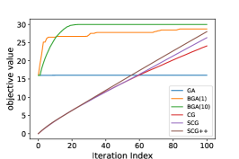
(a) Special Case

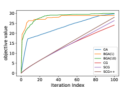
(b) Special Case (origin)

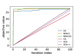
(c) Offline QP

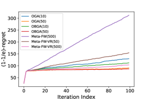
(d) Online QP with feedback delays

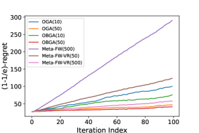
(e) Online QP without feedback delays

Figure 1: In  Figure 1(a), we test the performance of the six algorithms for the special submodular function in Hassani et al. (2017) where the GA, BGA and BGA(10) start from $\boldsymbol{x}_{loc}$. Simultaneously, we present the results for all algorithm starting from the origin in  Figure 1(b).  Figure 1(c) show the performance of the algorithms versus the number of iterations in a simulated Non-convex/Non-concave submodular QP. Finally,  Figure 1(d) and  Figure 1(e) show the $(1-1/e)$-regret of the seven algorithms, including OGA(10), OGA(50), OBGA(10), OBGA(50), Meta-FW(500), Meta-FW-VR(50), and Meta-FW-VR(500), for the simulated online submodular QP in both delayed setting and standard online setting.

5.1.1 Special Case

Hassani et al. (2017) introduced a special continuous DR-submodular function $f_{k}$ coming from the multilinear extension of a set cover function. Here, $f_{k}(\boldsymbol{x})=k+1-(1-x_{2k+1})\prod_{i=1}^{k}(1-x_{i})-(1-x_{2k+1})(k-\sum_{i=1}^{k}x_{i})+\sum_{i=k+1}^{2k}x_{i}$, where $\boldsymbol{x}=(x_{1},x_{2},\dots,x_{2k+1})$. Under the domain $\mathcal{C}=\{\boldsymbol{x}\in[0,1]^{2k+1}:\sum_{i=1}^{2k+1}x_{i}=k\}$, Hassani et al. (2017) also verified that $\boldsymbol{x}_{loc}=(\overbrace{1,1,\dots,1}^{k},0,\dots,0)$ is a local maximum with $(1/2+1/(2k))$-approximation to the global maximum. Thus, if start at $\boldsymbol{x}_{loc}$, theoretically Gradient Ascent (Hassani et al., 2017) will get stuck at this local maximum point. In our experiment, we set $k=15$ and consider a standard Gaussian noise, i.e., $[\widetilde{\nabla}f(x)]_{i}=[\nabla f(x)]_{i}+\mathcal{N}(0,1)$ for any $i\in[2k]$.

First, we set the initial point of GA, BGA(1) and BGA(10) to be $\boldsymbol{x}_{loc}$. From Figure 1(a), we observe that GA stays at $\boldsymbol{x}_{loc}$ as expected. Instead, BGA(1) and BGA(10) escape the local maximum $\boldsymbol{x}_{loc}$ and achieve near-optimal objective values. Then, we run all algorithms from the origin and present the results in Figure 1(b). It shows that GA, starting from the origin, performs much better than from a local maximum. Compared with GA, BGA(1) and BGA(10) converge to the optimal point $\boldsymbol{x}^{*}=(0,\dots,0,\overbrace{1,1,\dots,1}^{k+1})$ more rapidly. Both Figure 1(a) and Figure 1(b) show that BGA(1) and BGA(10) also perform better than Frank-Wolfe-type algorithms with respect to the convergence rate and the objective value.

5.1.2 Non-Convex/Non-Concave Quadratic Programming

We consider the quadratic objective $f(\boldsymbol{x})=\frac{1}{2}\boldsymbol{x}^{T}\boldsymbol{H}\boldsymbol{x}+\boldsymbol{h}^{T}\boldsymbol{x}$ and constraints $P=\{\boldsymbol{x}\in\mathbb{R}^{n}_{+}|\boldsymbol{A}\boldsymbol{x}\leq\boldsymbol{b},\boldsymbol{0}\leq\boldsymbol{x}\leq\boldsymbol{u},\boldsymbol{A}\in\mathbb{R}^{m\times n}_{+},\boldsymbol{b}\in\mathbb{R}_{+}^{m}\}$. Following Bian et al. (2017), we choose the matrix $\boldsymbol{H}\in\mathbb{R}^{n\times n}$ to be a randomly generated symmetric matrix with entries uniformly distributed in $[-1,0]$, and the matrix $\boldsymbol{A}$ to be a random matrix with entries uniformly distributed in $[0,1]$. It can be verified that $f$ is a continuous DR-submodular function. We also set $\boldsymbol{b}=\boldsymbol{u}=\boldsymbol{1}$, $m=12$, and $n=25$. To ensure the monotonicity, we set $\boldsymbol{h}=-\boldsymbol{H}^{T}\boldsymbol{u}$. Thus, the objective becomes $f(x)=(\frac{1}{2}\boldsymbol{x}-\boldsymbol{u})^{T}\boldsymbol{H}\boldsymbol{x}$. Similarly, we also consider the Gaussian noise for gradient, i.e., $[\widetilde{\nabla}f(\boldsymbol{x})]_{i}=[\nabla f(\boldsymbol{x})]_{i}+\delta\mathcal{N}(0,1)$ for any $i\in[n]$. We consider $\delta=5$ and start all algorithms from the origin.

As shown in Figure 1(c), BGA(1) and BGA(10) converge faster than GA and achieve nearly the same objective values as GA after $100$ iterations. Similar to the previous experiment, BGA(1) and BGA(10) exceed Frank-Wolfe-type algorithms with respect to the convergence rate.

5.2 Online Settings

We also consider Online DR-submodular Maximization with/without adversarial delays. Here, we present a list of algorithms to be compared in these settings:
Meta-Frank-Wolfe (Meta-FW($K$)): We consider Algorithm 1 in Chen et al. (2018b) and initialize $K$ online gradient descent oracles (Zinkevich, 2003; Hazan et al., 2016b) with step size $1/\sqrt{T}$.
Stochastic Meta-Frank-Wolfe (Meta-FW-VR($K$)): We consider Algorithm 1 in (Chen et al., 2018a) with the $\rho_{t}=1/(t+3)^{2/3}$ and $K$ online gradient descent oracles with step size $1/\sqrt{T}$.
Online Gradient Ascent (OGA($B$)): The delayed gradient ascent algorithm in (Quanrud and Khashabi, 2015) with step size $1/\sqrt{T}$. We use $B$ independent samples to estimate $\nabla f_{t}(\boldsymbol{x}_{t})$ at each round.
Online Boosting Gradient Ascent (OBGA($B$)): We consider Algorithm 3 with the step size $\eta_{t}=1/\sqrt{T}$ and use the average of $B$ independent samples to estimate the gradient at each round.

The same as Section 5.1.2, we first generate $T=100$ quadratic objective functions $f_{1},f_{2},\dots,f_{T}$. The symmetric random matrix $H_{t}$, corresponding to $f_{t}$, is uniformly generated from $[-1,0]^{n\times n}$ for $t=1,\ldots,T$, and the matrix $\boldsymbol{A}$ in constraint is randomly generated from the uniform distribution in $[0,1]^{m\times n}$. We also add the Gaussian noise for the gradient of each $f_{t}$, i.e., $[\widetilde{\nabla}f_{t}(\boldsymbol{x})]_{i}=[\nabla f_{t}(\boldsymbol{x})]_{i}+\delta\mathcal{N}(0,1)$ with $\delta=5$ for any $i\in[n]$. To simulate the feedback delays, we generate a uniform random number $d_{t}$ from $\{1,2,3,4,5\}$ for the stochastic gradient information of $f_{t}$.

We present the $(1-1/e)$-regret of algorithms for the delayed setting and the standard online setting (Hazan et al., 2016b) in Figure 1(d) and Figure 1(e), respectively. Under both scenarios, our proposed OBGA with sample size $B=50$ exhibits the lowest regret among all algorithms. With the same sample size $B=10$ and $50$, OBGA consistently achieves lower regrets than OGA, which confirms the effectiveness of our boosting framework.

6 Conclusion

In this paper, based on a novel non-oblivious function, we present a boosting framework, covering boosting gradient ascent and online boosting delayed gradient ascent, for the stochastic continuous submodular maximization problem, under both offline and online settings. In the offline scenario, our boosting gradient ascent provides $(1-e^{-\gamma}-\epsilon^{2})$-approximation guarantees after $O(1/\epsilon^{2})$ iterations. Under the online setting, we are the first to consider delayed feedback for online submodular maximization problems. Moreover, when no delay exists, our online boosting delayed gradient ascent is the first result to guarantee $(1-e^{-\gamma})$-approximation with $O(\sqrt{T})$ regret, where at each round we only estimate stochastic gradient $O(1)$ times. Numerical experiments demonstrate the superior performance of our algorithms.

A Proofs in Section 3

A.1 Proof of Lemma 1

First, we review some basic inequalities for $\gamma$-weakly continuous DR-submodular function $f$.

Lemma 3

For a monotone, differentiable, and $\gamma$-weakly continuous DR-submodular function $f$, we have

1. For any $\boldsymbol{x}\leq\boldsymbol{y}$, we have $\langle\boldsymbol{y}-\boldsymbol{x},\nabla f(\boldsymbol{x})\rangle\geq\gamma(f(\boldsymbol{y})-f(\boldsymbol{x}))$ and $\langle\boldsymbol{y}-\boldsymbol{x},\nabla f(\boldsymbol{y})\rangle\leq\frac{1}{\gamma}(f(\boldsymbol{y})-f(\boldsymbol{x}))$.

2. For any $\boldsymbol{x},\boldsymbol{y}\in\mathcal{X}$, we also could derive $\langle\boldsymbol{y}-\boldsymbol{x},\nabla f(\boldsymbol{x})\rangle\geq\gamma f(\boldsymbol{x}\lor\boldsymbol{y})+\frac{1}{\gamma}f(\boldsymbol{x}\land\boldsymbol{y})-(\gamma+\frac{1}{\gamma})f(\boldsymbol{x})$.

Proof  First, according to the definition of DR-submodular function and monotone property in Section 2, we have $\nabla f(\boldsymbol{x})\geq\gamma\nabla f(\boldsymbol{y})$, if $\boldsymbol{x}\leq\boldsymbol{y}$. Thus, for any $\boldsymbol{x}\leq\boldsymbol{y}$, we have

$$f(\boldsymbol{y})-f(\boldsymbol{x})=\int_{0}^{1}\langle\boldsymbol{y}-\boldsymbol{x},\nabla f(\boldsymbol{x}+z(\boldsymbol{y}-\boldsymbol{x}))\rangle dz\leq\frac{1}{\gamma}\langle\boldsymbol{y}-\boldsymbol{x},\nabla f(\boldsymbol{x}))\rangle,$$ (3)

$$f(\boldsymbol{y})-f(\boldsymbol{x})=\int_{0}^{1}\langle\boldsymbol{y}-\boldsymbol{x},\nabla f(\boldsymbol{x}+z(\boldsymbol{y}-\boldsymbol{x}))\rangle dz\geq\gamma\langle\boldsymbol{y}-\boldsymbol{x},\nabla f(\boldsymbol{y})\rangle,$$

where these two inequalities follow from $\boldsymbol{y}\geq\boldsymbol{x}+z(\boldsymbol{y}-\boldsymbol{x})\geq\boldsymbol{x}$ such that $\frac{1}{\gamma}\nabla f(\boldsymbol{x})\geq\nabla f(\boldsymbol{x}+z(\boldsymbol{y}-\boldsymbol{x}))\geq\gamma\nabla f(\boldsymbol{y})$ for any $z\in[0,1]$. We finish the proof of the first inequality in Lemma 3.

Then, from (3), we could derive that

$$\langle\boldsymbol{y}\lor\boldsymbol{x}-\boldsymbol{x},\nabla f(\boldsymbol{x})\rangle\geq\gamma f(\boldsymbol{y}\lor\boldsymbol{x})-\gamma f(\boldsymbol{x}),$$ (4)

$$\langle\boldsymbol{x}\land\boldsymbol{y}-\boldsymbol{x},\nabla f(\boldsymbol{x})\rangle\geq\frac{1}{\gamma}(f(\boldsymbol{x}\land\boldsymbol{y})-f(\boldsymbol{x})),$$

where $\boldsymbol{y}\lor\boldsymbol{x}\geq\boldsymbol{x}$ and $\boldsymbol{x}\land\boldsymbol{y}\leq\boldsymbol{x}$.

Merging the two equations in (4), we have, for any $\boldsymbol{x}$ and $\boldsymbol{y}\in\mathcal{X}$,

$$\langle\boldsymbol{y}-\boldsymbol{x},\nabla f(\boldsymbol{x})\rangle =\langle\boldsymbol{y}\lor\boldsymbol{x}-\boldsymbol{x},\nabla f(\boldsymbol{x})\rangle+\langle\boldsymbol{x}\land\boldsymbol{y}-\boldsymbol{x},\nabla f(\boldsymbol{x})\rangle$$ (5)

$$\geq\gamma f(\boldsymbol{x}\lor\boldsymbol{y})+\frac{1}{\gamma}f(\boldsymbol{x}\land\boldsymbol{y})-(\gamma+\frac{1}{\gamma})f(\boldsymbol{x}),$$

where $\boldsymbol{x}\land\boldsymbol{y}+\boldsymbol{x}\lor\boldsymbol{y}=\boldsymbol{x}+\boldsymbol{y}$. Thus, we prove the second inequality in Lemma 3.  

Next, with the Lemma 3, we prove the Lemma 1.

Proof From Equation 5, if $\boldsymbol{x}$ is a stationary point of $f$ in domain $\mathcal{C}$, we have $(\gamma+\frac{1}{\gamma})f(\boldsymbol{x})\geq\gamma f(\boldsymbol{x}\lor\boldsymbol{y})+\frac{1}{\gamma}f(\boldsymbol{x}\land\boldsymbol{y})$ for any $\boldsymbol{y}\in\mathcal{C}$. Due to the monotone and non-negative property, $f(\boldsymbol{x})\geq\frac{\gamma^{2}}{\gamma^{2}+1}\max_{\boldsymbol{y}\in\mathcal{C}}f(\boldsymbol{y})$.  

A.2 Proof of Lemma 2

Proof  First, we obtain an inequality about $\langle\boldsymbol{x},\nabla F(\boldsymbol{x})\rangle$, i.e.,

$$\langle\boldsymbol{x},\nabla F(\boldsymbol{x})\rangle =\int_{0}^{1}w(z)\langle\boldsymbol{x},\nabla f(z*\boldsymbol{x})\rangle\mathrm{d}z$$ (6)

$$=\int^{1}_{0}w(z)\mathrm{d}f(z*\boldsymbol{x})$$

$$=w(z)f(z*\boldsymbol{x})|_{z=0}^{z=1}-\int_{0}^{1}f(z*\boldsymbol{x})w^{\prime}(z)\mathrm{d}z$$

$$\leq w(1)f(\boldsymbol{x})-\int_{0}^{1}f(z*\boldsymbol{x})w^{\prime}(z)\mathrm{d}z.$$

Then, we also prove some properties about $\langle\boldsymbol{y},\nabla F(\boldsymbol{x})\rangle$, namely,

$$\langle\boldsymbol{y},\nabla F(\boldsymbol{x})\rangle =\int_{0}^{1}w(z)\langle\boldsymbol{y},\nabla f(z*\boldsymbol{x})\rangle\mathrm{d}z$$ (7)

$$\geq\int^{1}_{0}w(z)\langle\boldsymbol{y}\lor(z*\boldsymbol{x})-z*\boldsymbol{x},\nabla f(z*\boldsymbol{x})\rangle\mathrm{d}z$$

$$\geq\gamma\int^{1}_{0}w(z)(f(\boldsymbol{y}\lor(z*\boldsymbol{x}))-f(z*\boldsymbol{x}))\mathrm{d}z$$

$$\geq(\gamma\int_{0}^{1}w(z)dz)f(\boldsymbol{y})-\int^{1}_{0}\gamma w(z)f(z*\boldsymbol{x})\mathrm{d}z,$$

where the first inequality follows from $\boldsymbol{y}\geq\boldsymbol{y}\lor(z*\boldsymbol{x})-z*\boldsymbol{x}\geq\boldsymbol{0}$ and $\nabla f(z*\boldsymbol{x})\geq\boldsymbol{0}$; the second one comes from the Lemma 1; and the final inequality follows from $f(\boldsymbol{y}\lor(z*\boldsymbol{x}))\geq f(\boldsymbol{y})$.

Finally, putting above the inequality (6) and inequality (7) together, we have

$$\langle\boldsymbol{y}-\boldsymbol{x},\nabla F(\boldsymbol{x})\rangle \geq(\gamma\int_{0}^{1}w(z)\mathrm{d}z)f(\boldsymbol{y})-w(1)f(\boldsymbol{x})+\int^{1}_{0}(w^{\prime}(z)-\gamma w(z))f(z*\boldsymbol{x})\mathrm{d}z$$ (8)

$$=(\gamma\int_{0}^{1}w(z)\mathrm{d}z)(f(\boldsymbol{y})-\frac{w(1)+\int^{1}_{0}(\gamma w(z)-w^{\prime}(z))\frac{f(z*\boldsymbol{x})}{f(\boldsymbol{x})}\mathrm{d}z}{\gamma\int_{0}^{1}w(z)\mathrm{d}z}f(\boldsymbol{x}))$$

$$=(\gamma\int_{0}^{1}w(z)\mathrm{d}z)(f(\boldsymbol{y})-\theta(w,f,\boldsymbol{x})f(\boldsymbol{x}))$$

$$\geq(\gamma\int_{0}^{1}w(z)\mathrm{d}z)(f(\boldsymbol{y})-\theta(w)f(\boldsymbol{x})),$$

where the final inequality follows from $\theta(w)=\max_{f,\boldsymbol{x}}\theta(w,f,\boldsymbol{x})$.  

A.3 Proof of Theorem 1

Proof  In this proof, we investigate the optimal value and solution about the following optimization problem:

$$\min_{w}\theta(w)=\min_{w}\max_{f,\boldsymbol{x}} \frac{w(1)+\int^{1}_{0}(\gamma w(z)-w^{\prime}(z))\frac{f(z*\boldsymbol{x})}{f(\boldsymbol{x})}\mathrm{d}z}{\gamma\int_{0}^{1}w(z)\mathrm{d}z}$$ (9)

$$\rm{s.t.} w(z)\geq 0,$$

$$w(z)\in C^{1}[0,1],$$

$$f(\boldsymbol{x})>0,$$

$$\nabla f(\boldsymbol{x}_{1})\geq\gamma\nabla f(\boldsymbol{y}_{1})\geq\boldsymbol{0},\forall\boldsymbol{x}_{1}\leq\boldsymbol{y}_{1}.$$

(1) Before going into the detail, we first consider a new optimization problem as follows:

$$\min_{w}\max_{R} \theta(w,R)$$ (10)

$$\rm{s.t.} w(z)\geq 0,$$

$$w(z)\in C^{1}[0,1],$$

$$\gamma\int_{0}^{1}w(z)dz=1,$$

$$R(z)\geq 0,$$

$$R(1)=1,$$

$$R^{\prime}(z_{1})\geq\gamma R^{\prime}(z_{2})\geq 0\ (\forall z_{1}\leq z_{2},z_{1},z_{2}\in[0,1]),$$

where $\theta(w,R)=w(1)+\int^{1}_{0}(\gamma w(z)-w^{\prime}(z))R(z)\mathrm{d}z$.

Next, we prove the equivalence between problem (9) and problem (10). For any fixed point $\boldsymbol{x}\in\mathcal{C}$, we consider the function $m(z)=\frac{f(z*\boldsymbol{x})}{f(\boldsymbol{x})}$ (we assume $f(\boldsymbol{x})>0$), which is satisfied with the constraints of problem (10), i.e., $m(z)\geq 0$, $m(1)=1$, and $m^{\prime}(z_{1})=\frac{\langle\boldsymbol{x},\nabla f(z_{1}*\boldsymbol{x})\rangle}{f(\boldsymbol{x})}\geq\frac{\gamma\langle\boldsymbol{x},\nabla f(z_{2}*\boldsymbol{x})\rangle}{f(\boldsymbol{x})}=\gamma m^{\prime}(z_{2})\geq 0$ $(\forall z_{1}\leq z_{2},z_{1},z_{2}\in[0,1])$. Therefore, the optimal objective value of problem (10) is larger than that of problem (9). Moreover, for any $R(z)$ satisfying the constrains in problem (10), we can design a function $f_{1}(\boldsymbol{x})=R(x_{1}/a_{1})$, where $x_{1}$ (we assume $x_{1}\in[0,a_{1}]$ in the Section 2) is the first coordinate of point $\boldsymbol{x}$. Also, $f_{1}(\boldsymbol{x})\geq 0$ and when $\boldsymbol{x}\leq\boldsymbol{y}$, we have $\nabla f_{1}(\boldsymbol{x})\geq\gamma\nabla f_{1}(\boldsymbol{y})$. Hence, $f_{1}$ is also satisfied with the constraints of problem (9). If we set $\boldsymbol{x}_{1}=(a_{1},0,\dots,0)\in\mathcal{X}$, $\frac{f_{1}(z*\boldsymbol{x}_{1})}{f_{1}(\boldsymbol{x}_{1})}=R(z)$ such that the optimal objective value of problem (9) is larger than that of problem (10). As a result, the optimization problem (10) is equivalent to the problem (9).

(2) Then, we prove the $\min_{w}\max_{f,\boldsymbol{x}}\theta(w,f,\boldsymbol{x})\geq\frac{1}{1-e^{-\gamma}}$. Setting $\widehat{R}(z)=\frac{1-e^{-\gamma z}}{1-e^{-\gamma}}$, we could verify that, if $\gamma\int_{0}^{1}w(z)dz=1$,

$$\theta(w,\widehat{R}) =w(1)+\int^{1}_{0}(\gamma w(z)-w^{\prime}(z))\widehat{R}(z)\mathrm{d}z$$ (11)

$$=w(1)+\frac{\int^{1}_{0}(\gamma w(z)-w^{\prime}(z))\mathrm{d}z+\int^{1}_{0}e^{-\gamma z}(w^{\prime}(z)-\gamma w(z))\mathrm{d}z}{1-e^{-\gamma}}$$

$$=w(1)+\frac{1-w(1)+w(0)+e^{-\gamma z}w(z)|_{z=0}^{z=1}}{1-e^{-\gamma}}$$

$$=w(1)+\frac{1-w(1)+w(0)+e^{-\gamma}w(1)-w(0)}{1-e^{-\gamma}}$$

$$=\frac{1}{1-e^{-\gamma}}.$$

Also, $\widehat{R}$ is satisfied with the constraints of optimization problem (10), i.e., for any $z\in[0,1]$, $\widehat{R}(z)\geq 0$, $\widehat{R}(1)=1$ and $\widehat{R}^{\prime}(x)=\frac{\gamma e^{-\gamma x}}{1-e^{-\gamma}}\geq\frac{\gamma^{2}e^{-\gamma y}}{1-e^{-\gamma}}=\gamma\widehat{R}^{\prime}(y)$ where $x\leq y$ and $0\leq\gamma\leq 1$. Therefore, $\max_{R}\theta(w,R)\geq\theta(w,\widehat{R})=\frac{1}{1-e^{-\gamma}}$ and $\min_{w}\max_{f,\boldsymbol{x}}\theta(w,f,\boldsymbol{x})=\min_{w}\max_{R}\theta(w,R)\geq\frac{1}{1-e^{-\gamma}}$.

(3) We consider $\widehat{w}(z)=e^{\gamma(z-1)}$ and observe that $\widehat{w}^{\prime}(z)=\gamma\widehat{w}(z)$ such that $\theta(\widehat{w},f,\boldsymbol{x})=\frac{\widehat{w}(1)+\int^{1}_{0}(\gamma\widehat{w}(z)-\widehat{w}^{\prime}(z))\frac{f(z*\boldsymbol{x})}{f(\boldsymbol{x})}\mathrm{d}z}{\gamma\int_{0}^{1}\widehat{w}(z)\mathrm{d}z}=\frac{\widehat{w}(1)}{\gamma\int_{0}^{1}\widehat{w}(z)\mathrm{d}z}=\frac{1}{1-e^{-\gamma}}$ for any function $f$. Also, $\widehat{w}(z)$ is satisfied with the constraints in optimization problem (9), namely, $\widehat{w}(z)\geq 0$ and $\widehat{w}\in C^{1}[0,1]$. Therefore, $\frac{1}{1-e^{-\gamma}}=\min_{w}\max_{f,\boldsymbol{x}}\theta(w,f,\boldsymbol{x})$ and $e^{\gamma(z-1)}\in\arg\min_{w}\theta(w)$.  

A.4 Proof of Theorem 2

Proof  From the definition of $F$, we have $\langle\boldsymbol{y}-\boldsymbol{x},\nabla F(\boldsymbol{x})\rangle\geq(1-e^{-\gamma})f(\boldsymbol{y})-f(\boldsymbol{x})$ for any point $\boldsymbol{x},\boldsymbol{y}\in\mathcal{C}$. Hence, when $\boldsymbol{x}\in\mathcal{C}$ is a stationary point for $F$ in the domain $\mathcal{C}$, $0\geq\langle\boldsymbol{y}-\boldsymbol{x},\nabla F(\boldsymbol{x})\rangle\geq(1-e^{-\gamma})f(\boldsymbol{y})-f(\boldsymbol{x})$ for any point $\boldsymbol{y}\in\mathcal{C}$ such that $f(\boldsymbol{x})\geq(1-e^{-\gamma})\max_{\boldsymbol{y}\in\mathcal{C}}f(\boldsymbol{y})$.

Then, for the second one, we first verify that the value $\int_{0}^{1}\frac{e^{\gamma(z-1)}}{z}f(z*\boldsymbol{x})\mathrm{d}z$ is controlled via $f(\boldsymbol{x})$ for any $\boldsymbol{x}\in\mathcal{X}$. For any $\delta\in(0,1)$, we first have

$$\int_{0}^{1}\frac{e^{\gamma(z-1)}}{z}f(z*\boldsymbol{x})\mathrm{d}z$$ (12)

$$=(\int_{0}^{\delta}+\int_{\delta}^{1})\frac{e^{\gamma(z-1)}}{z}f(z*\boldsymbol{x})\mathrm{d}z$$

$$\leq\int_{0}^{\delta}\frac{f(z*x)}{z}\mathrm{d}z+(\int_{\delta}^{1}\frac{1}{z}\mathrm{d}z)f(\boldsymbol{x})$$

$$=\int_{0}^{\delta}\frac{f(z*x)}{z}\mathrm{d}z+\ln(\frac{1}{\delta})f(\boldsymbol{x})$$

$$=\int_{0}^{\delta}\frac{\int_{0}^{z}\langle\boldsymbol{x},\nabla f(u*\boldsymbol{x})\rangle\mathrm{d}u}{z}\mathrm{d}z+\ln(\frac{1}{\delta})f(\boldsymbol{x}),$$

where the first inequality follows from $f(z*\boldsymbol{x})\leq f(\boldsymbol{x})$ and $\delta\in[0,1]$, and the final equality from $\int_{0}^{z}\langle\boldsymbol{x},\nabla f(u*\boldsymbol{x})\rangle\mathrm{d}u=f(z*\boldsymbol{x})-f(\boldsymbol{0})=f(z*\boldsymbol{x})$.

Next,

$$\int_{0}^{\delta}\frac{\int_{0}^{z}\langle\boldsymbol{x},\nabla f(u*\boldsymbol{x})\rangle\mathrm{d}u}{z}\mathrm{d}z =\int_{0}^{\delta}\langle\boldsymbol{x},\nabla f(u*\boldsymbol{x})\rangle\int_{u}^{\delta}\frac{1}{z}\mathrm{d}z\mathrm{d}u$$ (13)

$$=\int_{0}^{\delta}\langle\boldsymbol{x},\nabla f(u*\boldsymbol{x})\rangle\ln(\frac{\delta}{u})\mathrm{d}u$$

$$=\int_{0}^{\delta}(\langle\boldsymbol{x},\nabla f(u*\boldsymbol{x})-\nabla f(\boldsymbol{x})\rangle+\langle\boldsymbol{x},\nabla f(\boldsymbol{x})\rangle)\ln(\frac{\delta}{u})\mathrm{d}u$$

$$\leq\int_{0}^{\delta}\ln(\frac{\delta}{u})\mathrm{d}u(Lr^{2}(\mathcal{X})+\frac{f(\boldsymbol{x})}{\gamma})$$

$$=(u-u\ln(\frac{u}{\delta}))|_{u=0}^{\delta}(Lr^{2}(\mathcal{X})+\frac{f(\boldsymbol{x})}{\gamma})$$

$$=\delta(Lr^{2}(\mathcal{X})+\frac{f(\boldsymbol{x})}{\gamma}),$$

where the first equality follows from the Fubini’s theorem; in the first inequality, we use $\langle\boldsymbol{x},\nabla f(u*\boldsymbol{x})-\nabla f(\boldsymbol{x})\rangle\leq L\left\|\boldsymbol{x}\right\|^{2}$, which is derived from the $L$-smooth property, and $\langle\boldsymbol{x},\nabla f(\boldsymbol{x})\rangle\leq\frac{f(\boldsymbol{x})}{\gamma}$, following from the Lemma 1 and $f(\boldsymbol{0})=0$; the final equality follows from $\lim_{u\rightarrow 0_{+}}u\ln(u)=0$.

From Equation 12 and Equation 13, for any $\delta\in(0,1)$, we have

$$F(\boldsymbol{x}) \leq\ln(\frac{1}{\delta})f(\boldsymbol{x})+\delta(L_{*}r^{2}(\mathcal{X})+\frac{f(\boldsymbol{x})}{\gamma})$$ (14)

$$\leq\ln(\frac{1}{\delta})(f(\boldsymbol{x})+c)+\delta(L_{*}r^{2}(\mathcal{X})+\frac{f(\boldsymbol{x})}{\gamma}),$$

where the second inequality comes from $c>0$.

If we set $\delta=\frac{f(\boldsymbol{x})+c}{\frac{f(\boldsymbol{x})}{\gamma}+Lr^{2}(\mathcal{X})}\in[0,1]$ ($0\leq\gamma\leq 1$ and $0<c\leq L_{*}r^{2}(\mathcal{X})$), we have

$$F(\boldsymbol{x}) \leq\ln(\frac{1}{\delta})(f(\boldsymbol{x})+c)+\delta(L_{*}r^{2}(\mathcal{X})+\frac{f(\boldsymbol{x})}{\gamma})$$

$$=(1+\ln(\frac{1}{\delta}))(f(\boldsymbol{x})+c)$$

$$\leq(1+\ln(\tau)(f(\boldsymbol{x})+c),$$

where the final inequality is derived from $\frac{1}{\delta}\leq\tau$ and $\tau=max(\frac{1}{\gamma},\frac{L_{*}r^{2}(\mathcal{X})}{c})$.

As a result, the value $\int_{0}^{1}\frac{e^{\gamma(z-1)}}{z}f(z*\boldsymbol{x})\mathrm{d}z$ is well-defined. We also could verify that $\nabla\int_{0}^{1}\frac{e^{\gamma(z-1)}}{z}f(z*\boldsymbol{x})\mathrm{d}z=\int_{0}^{1}e^{\gamma(z-1)}\nabla f(z*\boldsymbol{x})\mathrm{d}z$ so that we could set $F(\boldsymbol{x})=\int_{0}^{1}\frac{e^{\gamma(z-1)}}{z}f(z*\boldsymbol{x})\mathrm{d}z$.

For the final one,

$$\left\|\nabla F(\boldsymbol{x})-\nabla F(\boldsymbol{y})\right\| =\left\|\int_{0}^{1}e^{\gamma(z-1)}(\nabla f(z*\boldsymbol{x})-\nabla f(z*\boldsymbol{y}))\mathrm{d}z\right\|$$ (15)

$$\leq\int_{0}^{1}e^{\gamma(z-1)}\left\|\nabla f(z*\boldsymbol{x})-\nabla f(z*\boldsymbol{y})\right\|\mathrm{d}z$$

$$\leq L(\int_{0}^{1}e^{\gamma(z-1)}zdz)\left\|\boldsymbol{x}-\boldsymbol{y}\right\|$$

$$=\frac{\gamma+e^{-\gamma}-1}{\gamma^{2}}L\left\|\boldsymbol{x}-\boldsymbol{y}\right\|.$$

 

A.5 Proof of Proposition 1

Proof  For the first one, fixed $z$, $\mathbb{E}\left(\left.\widetilde{\nabla}f(z*\boldsymbol{x})\right|\boldsymbol{x},z\right)=\nabla f(z*\boldsymbol{x})$ such that $\mathbb{E}\left(\left.\widetilde{\nabla}f(z*\boldsymbol{x})\right|\boldsymbol{x}\right)=\mathbb{E}_{z\sim\mathbf{Z}}\left(\mathbb{E}\left(\left.\widetilde{\nabla}f(z*\boldsymbol{x})\right|\boldsymbol{x},z\right)\right)=\mathbb{E}_{z\sim\mathbf{Z}}\left(\left.\nabla f(z*\boldsymbol{x})\right|\boldsymbol{x}\right)=\int_{z=0}^{1}\frac{\gamma e^{\gamma(z-1)}}{1-e^{-\gamma}}\nabla f(z*\boldsymbol{x})\mathrm{d}z=\frac{\gamma}{1-e^{-\gamma}}F(\boldsymbol{x})$. For the second one,

$$\mathbb{E}\left(\left.\left\|\frac{1-e^{-\gamma}}{\gamma}\widetilde{\nabla}f(z*\boldsymbol{x})-\nabla F(\boldsymbol{x})\right\|^{2}\right|\boldsymbol{x}\right)$$

$$= \mathbb{E}\left(\left.\left\|\frac{1-e^{-\gamma}}{\gamma}(\widetilde{\nabla}f(z*\boldsymbol{x})-\nabla f(z*\boldsymbol{x}))+\frac{1-e^{-\gamma}}{\gamma}\nabla f(z*\boldsymbol{x})-\nabla F(\boldsymbol{x})\right\|^{2}\right|\boldsymbol{x}\right)$$

$$\leq 2\mathbb{E}_{z\sim\mathbf{Z}}\left(\mathbb{E}\left(\left.\left\|\frac{1-e^{-\gamma}}{\gamma}(\widetilde{\nabla}f(z*\boldsymbol{x})-\nabla f(z*\boldsymbol{x}))\right\|^{2}\right|\boldsymbol{x},z\right)+\left\|\frac{1-e^{-\gamma}}{\gamma}\nabla f(z*\boldsymbol{x})-\nabla F(\boldsymbol{x})\right\|^{2}\right)$$

$$\leq 2\frac{(1-e^{-\gamma})^{2}\sigma^{2}}{\gamma^{2}}+2\mathbb{E}_{z\sim\mathbf{Z}}\left(\left.\left\|\frac{1-e^{-\gamma}}{\gamma}\nabla f(z*\boldsymbol{x})-\nabla F(\boldsymbol{x})\right\|^{2}\right|\boldsymbol{x}\right)$$

$$\leq 2\frac{(1-e^{-\gamma})^{2}\sigma^{2}}{\gamma^{2}}+2\mathbb{E}_{z\sim\mathbf{Z}}\left(\left.\left\|\int_{0}^{1}e^{\gamma(u-1)}(\nabla f(z*\boldsymbol{x})-\nabla f(u*\boldsymbol{x}))\mathrm{d}u\right\|^{2}\right|\boldsymbol{x}\right)$$

$$\leq 2\frac{(1-e^{-\gamma})^{2}\sigma^{2}}{\gamma^{2}}+2\mathbb{E}_{z\sim\mathbf{Z}}\left(\left.\left(\int_{0}^{1}e^{\gamma(u-1)}|z-u|L\left\|\boldsymbol{x}\right\|\mathrm{d}u\right)^{2}\right|\boldsymbol{x}\right)$$

$$\leq 2\frac{(1-e^{-\gamma})^{2}\sigma^{2}}{\gamma^{2}}+2\mathbb{E}_{z\sim\mathbf{Z}}\left(\left.\int_{0}^{1}e^{\gamma(u-1)}\mathrm{d}u\int_{u=0}^{1}e^{\gamma(u-1)}(z-u)^{2}L^{2}\left\|\boldsymbol{x}\right\|^{2}\mathrm{d}u\right|\boldsymbol{x}\right)$$

$$= 2\frac{(1-e^{-\gamma})^{2}\sigma^{2}}{\gamma^{2}}+2\int_{z=0}^{1}\int_{u=0}^{1}e^{\gamma(u+z-2)}(z-u)^{2}L^{2}\left\|\boldsymbol{x}\right\|^{2}\mathrm{d}u\mathrm{d}z$$

$$\leq 2\frac{(1-e^{-\gamma})^{2}\sigma^{2}}{\gamma^{2}}+\frac{2L^{2}r^{2}(\mathcal{X})(1-e^{-2\gamma})}{3\gamma},$$

where the first and fifth inequalities come from Cauchy–Schwarz inequality.  

B Proof of Theorem 3

First, we recall the projection theorem from (Bertsekas, 2015) in the following lemma.

Lemma 4

For the projection $\mathcal{P}_{\mathcal{C}}(\boldsymbol{x})=\arg\min_{\boldsymbol{z}\in\mathcal{C}}\left\|\boldsymbol{z}-\boldsymbol{x}\right\|$, we have

$$\langle\mathcal{P}_{\mathcal{C}}(\boldsymbol{x}))-\boldsymbol{x},\boldsymbol{z}-\mathcal{P}_{\mathcal{C}}(\boldsymbol{x})\rangle\geq 0,\forall\boldsymbol{z}\in\mathcal{C}.$$ (16)

Before verifying the Theorem 3, we first provide following lemma.

Lemma 5

In the $t$-round update in  Algorithm 2, if we set the $\widetilde{\nabla}F(\boldsymbol{x}_{t})=\frac{1-e^{-\gamma}}{\gamma}\widetilde{\nabla}f(z_{t}*\boldsymbol{x}_{t})$, for any $\boldsymbol{y}\in\mathcal{C}$ and $\mu_{t}>0$, we have

$$\mathbb{E}\left(F(\boldsymbol{x}_{t+1})-F(\boldsymbol{x}_{t})+f(\boldsymbol{x}_{t})-(1-e^{-\gamma})f(\boldsymbol{y})\right)$$

$$\geq \mathbb{E}\left(\frac{1}{2\eta_{t}}(\left\|\boldsymbol{y}-\boldsymbol{x}_{t+1}\right\|^{2}-\left\|\boldsymbol{y}-\boldsymbol{x}_{t}\right\|^{2})-\frac{1}{2\mu_{t}}\left\|\nabla F(\boldsymbol{x}_{t})-\widetilde{\nabla}F(\boldsymbol{x}_{t})\right\|^{2}+(\frac{1}{2\eta_{t}}-\frac{\mu_{t}+L_{\gamma}}{2})\left\|\boldsymbol{x}_{t+1}-\boldsymbol{x}_{t})\right\|^{2}\right).$$

Proof  From the Theorem 2, when $f$ is $L$-$smooth$, the non-oblivious function $F$ is $L_{\gamma}$-$smooth$. Hence

$$F(\boldsymbol{x}_{t+1})-F(\boldsymbol{x}_{t}) =\int_{z=0}^{z=1}\langle\boldsymbol{x}_{t+1}-\boldsymbol{x}_{t},\nabla F(\boldsymbol{x}_{t}+z(\boldsymbol{x}_{t+1}-\boldsymbol{x}_{t}))\rangle dz$$ (17)

$$\geq\langle\boldsymbol{x}_{t+1}-\boldsymbol{x}_{t},\nabla F(\boldsymbol{x}_{t})\rangle-\frac{L_{\gamma}}{2}\left\|\boldsymbol{x}_{t+1}-\boldsymbol{x}_{t}\right\|^{2}.$$

Then,

$$\langle\boldsymbol{x}_{t+1}-\boldsymbol{x}_{t},\nabla F(\boldsymbol{x}_{t})\rangle$$ (18)

$$= \langle\boldsymbol{x}_{t+1}-\boldsymbol{x}_{t},\widetilde{\nabla}F(\boldsymbol{x}_{t})\rangle+\langle\boldsymbol{x}_{t+1}-\boldsymbol{x}_{t},\nabla F(\boldsymbol{x}_{t})-\widetilde{\nabla}F(\boldsymbol{x}_{t})\rangle$$

$$\geq \langle\boldsymbol{x}_{t+1}-\boldsymbol{x}_{t},\widetilde{\nabla}F(\boldsymbol{x}_{t})\rangle-\frac{1}{2\mu_{t}}\left\|\nabla F(\boldsymbol{x}_{t})-\widetilde{\nabla}F(\boldsymbol{x}_{t})\right\|^{2}-\frac{\mu_{t}}{2}\left\|\boldsymbol{x}_{t+1}-\boldsymbol{x}_{t}\right\|^{2},$$

where the first inequality from the Young’s inequality.

It is well known $\widetilde{\nabla}F(\boldsymbol{x}_{t})=\frac{1}{\eta_{t}}(\boldsymbol{y}_{t+1}-\boldsymbol{x}_{t})$ such that

$$\langle\boldsymbol{x}_{t+1}-\boldsymbol{x}_{t},\widetilde{\nabla}F(\boldsymbol{x}_{t})\rangle$$ (19)

$$= \langle\boldsymbol{x}_{t+1}-\boldsymbol{y},\widetilde{\nabla}F(\boldsymbol{x}_{t})\rangle+\langle\boldsymbol{y}-\boldsymbol{x}_{t},\widetilde{\nabla}F(\boldsymbol{x}_{t})\rangle$$

$$= \frac{1}{\eta_{t}}\langle\boldsymbol{x}_{t+1}-\boldsymbol{y},\boldsymbol{y}_{t+1}-\boldsymbol{x}_{t}\rangle+\langle\boldsymbol{y}-\boldsymbol{x}_{t},\widetilde{\nabla}F(\boldsymbol{x}_{t})\rangle$$

$$= \frac{1}{\eta_{t}}\langle\boldsymbol{x}_{t+1}-\boldsymbol{y},\boldsymbol{y}_{t+1}-\boldsymbol{x}_{t+1}\rangle+\frac{1}{\eta_{t}}\langle\boldsymbol{x}_{t+1}-\boldsymbol{y},\boldsymbol{x}_{t+1}-\boldsymbol{x}_{t}\rangle+\langle\boldsymbol{y}-\boldsymbol{x}_{t},\widetilde{\nabla}F(\boldsymbol{x}_{t})\rangle$$

$$\geq \frac{1}{\eta_{t}}\langle\boldsymbol{x}_{t+1}-\boldsymbol{y},\boldsymbol{x}_{t+1}-\boldsymbol{x}_{t}\rangle+\langle\boldsymbol{y}-\boldsymbol{x}_{t},\widetilde{\nabla}F(\boldsymbol{x}_{t})\rangle$$

$$= \frac{1}{2\eta_{t}}(\left\|\boldsymbol{y}-\boldsymbol{x}_{t+1}\right\|^{2}+\left\|\boldsymbol{x}_{t+1}-\boldsymbol{x}_{t}\right\|^{2}-\left\|\boldsymbol{y}-\boldsymbol{x}_{t}\right\|^{2})+\langle\boldsymbol{y}-\boldsymbol{x}_{t},\widetilde{\nabla}F(\boldsymbol{x}_{t})\rangle,$$

where the first inequality follows from the  Lemma 4.

From the Equation (17)-(19), we have

$$F(\boldsymbol{x}_{t+1})-F(\boldsymbol{x}_{t})$$ (20)

$$\geq \frac{1}{2\eta_{t}}(\left\|\boldsymbol{y}-\boldsymbol{x}_{t+1}\right\|^{2}+\left\|\boldsymbol{x}_{t+1}-\boldsymbol{x}_{t}\right\|^{2}-\left\|\boldsymbol{y}-\boldsymbol{x}_{t}\right\|^{2})+\langle\boldsymbol{y}-\boldsymbol{x}_{t},\widetilde{\nabla}F(\boldsymbol{x}_{t})\rangle$$

$$-\frac{1}{2\mu_{t}}\left\|\nabla F(\boldsymbol{x}_{t})-\widetilde{\nabla}F(\boldsymbol{x}_{t})\right\|^{2}-\frac{\mu_{t}+L_{\gamma}}{2}\left\|\boldsymbol{x}_{t+1}-\boldsymbol{x}_{t}\right\|^{2}$$

$$\geq \frac{1}{2\eta_{t}}(\left\|\boldsymbol{y}-\boldsymbol{x}_{t+1}\right\|^{2}-\left\|\boldsymbol{y}-\boldsymbol{x}_{t}\right\|^{2})+\langle\boldsymbol{y}-\boldsymbol{x}_{t},\widetilde{\nabla}F(\boldsymbol{x}_{t})\rangle$$

$$-\frac{1}{2\mu_{t}}\left\|\nabla F(\boldsymbol{x}_{t})-\widetilde{\nabla}F(\boldsymbol{x}_{t})\right\|^{2}+(\frac{1}{2\eta_{t}}-\frac{\mu_{t}+L_{\gamma}}{2})\left\|\boldsymbol{x}_{t+1}-\boldsymbol{x}_{t}\right\|^{2}.$$

From the Proposition 1, $\mathbb{E}(\widetilde{\nabla}F(\boldsymbol{x}_{t})|\boldsymbol{x}_{t})=\nabla F(\boldsymbol{x}_{t})$ and we also have

$$\mathbb{E}\left(F(\boldsymbol{x}_{t+1})-F(\boldsymbol{x}_{t})\right)$$ (21)

$$\geq \mathbb{E}(\frac{1}{2\eta_{t}}(\left\|\boldsymbol{y}-\boldsymbol{x}_{t+1}\right\|^{2}-\left\|\boldsymbol{y}-\boldsymbol{x}_{t}\right\|^{2})+\mathbb{E}(\langle\boldsymbol{y}-\boldsymbol{x}_{t},\widetilde{\nabla}F(\boldsymbol{x}_{t})\rangle|\boldsymbol{x}_{t})$$

$$-\frac{1}{2\mu_{t}}\left\|\nabla F(\boldsymbol{x}_{t})-\widetilde{\nabla}F(\boldsymbol{x}_{t})\right\|^{2}+(\frac{1}{2\eta_{t}}-\frac{\mu_{t}+L_{\gamma}}{2})\left\|\boldsymbol{x}_{t+1}-\boldsymbol{x}_{t}\right\|^{2})$$

$$= \mathbb{E}(\frac{1}{2\eta_{t}}(\left\|\boldsymbol{y}-\boldsymbol{x}_{t+1}\right\|^{2}-\left\|\boldsymbol{y}-\boldsymbol{x}_{t}\right\|^{2})+\langle\boldsymbol{y}-\boldsymbol{x}_{t},\nabla F(\boldsymbol{x}_{t})\rangle$$

$$-\frac{1}{2\mu_{t}}\left\|\nabla F(\boldsymbol{x}_{t})-\widetilde{\nabla}F(\boldsymbol{x}_{t})\right\|^{2}+(\frac{1}{2\eta_{t}}-\frac{\mu_{t}+L_{\gamma}}{2})\left\|\boldsymbol{x}_{t+1}-\boldsymbol{x}_{t}\right\|^{2})$$

$$\geq \mathbb{E}(\frac{1}{2\eta_{t}}(\left\|\boldsymbol{y}-\boldsymbol{x}_{t+1}\right\|^{2}-\left\|\boldsymbol{y}-\boldsymbol{x}_{t}\right\|^{2})+(1-e^{-\gamma})f(\boldsymbol{y})-f(\boldsymbol{x}_{t})$$

$$-\frac{1}{2\mu_{t}}\left\|\nabla F(\boldsymbol{x}_{t})-\widetilde{\nabla}F(\boldsymbol{x}_{t})\right\|^{2}+(\frac{1}{2\eta_{t}}-\frac{\mu_{t}+L_{\gamma}}{2})\left\|\boldsymbol{x}_{t+1}-\boldsymbol{x}_{t}\right\|^{2}),$$

where the final inequality from the definition of $F$.  
Next, we prove the Theorem 3.

Proof  From the Lemma 5, if we set $\boldsymbol{y}=\boldsymbol{x}^{*}=\arg\max_{\boldsymbol{x}\in\mathcal{C}}f(\boldsymbol{x})$, we have

$$\sum_{t=1}^{T-1}\mathbb{E}(F(\boldsymbol{x}_{t+1})-F(\boldsymbol{x}_{t})+f(\boldsymbol{x}_{t})-(1-e^{-\gamma})f(\boldsymbol{x}^{*}))$$ (22)

$$\geq \sum_{t=1}^{T-1}\mathbb{E}(\frac{1}{2\eta_{t}}(\left\|\boldsymbol{x}^{*}-\boldsymbol{x}_{t+1}\right\|^{2}-\left\|\boldsymbol{x}^{*}-\boldsymbol{x}_{t}\right\|^{2})-\sum_{t=1}^{T-1}\frac{1}{2\mu_{t}}\left\|\nabla F(\boldsymbol{x}_{t})-\widetilde{\nabla}F(\boldsymbol{x}_{t})\right\|^{2})$$

$$\geq -\sigma_{\gamma}^{2}\sum_{t=1}^{T}\frac{1}{2\mu_{t}}+\sum_{t=2}^{T-1}\mathbb{E}(\left\|\boldsymbol{x}^{*}-\boldsymbol{x}_{t}\right\|^{2})(\frac{1}{2\eta_{t-1}}-\frac{1}{2\eta_{t}})+\mathbb{E}(\frac{\left\|\boldsymbol{x}^{*}-\boldsymbol{x}_{T}\right\|^{2}}{2\eta_{T-1}}-\frac{\left\|\boldsymbol{x}^{*}-\boldsymbol{x}_{1}\right\|^{2}}{2\eta_{1}})$$

$$\geq -\frac{\mathrm{diam}^{2}(\mathcal{C})}{2\eta_{T-1}}-\sigma_{\gamma}^{2}\sum_{t=1}^{T}\frac{1}{\mu_{t}}$$

$$\geq -(\mathrm{diam}^{2}(\mathcal{C})L_{\gamma}/2+3\sigma_{\gamma}\mathrm{diam}(\mathcal{C})\sqrt{T}/2)$$

where the first inequality follows from $\eta_{t}=\frac{1}{\mu_{t}+L_{r}}$ if we set $\mu_{t}=\frac{\sigma_{\gamma}\sqrt{t}}{\mathrm{diam}(\mathcal{C})}$ in Lemma 5; the second inequality from the Proposition 1 and the Abel’s inequality; the third inequality from the definition of $\mathrm{diam}(\mathcal{C})$.

Finally, we have:

$$\mathbb{E}(\sum_{t=1}^{T-1}f(\boldsymbol{x}_{t})+F(\boldsymbol{x}_{T}))\geq(1-e^{-\gamma})(T-1)f(\boldsymbol{x}^{*})-(\mathrm{diam}^{2}(\mathcal{C})L_{\gamma}/2+3\sigma_{\gamma}\mathrm{diam}(\mathcal{C})\sqrt{T}/2)$$ (23)

According to Theorem 2,

$$\mathbb{E}(\sum_{t=1}^{T-1}f(\boldsymbol{x}_{t})+(1+\log(\tau))(f(\boldsymbol{x}_{T})+c)\geq(1-e^{-\gamma})(T-1)f(\boldsymbol{x}^{*})-(\mathrm{diam}^{2}(\mathcal{C})L_{\gamma}/2+3\sigma_{\gamma}\mathrm{diam}(\mathcal{C})\sqrt{T}/2)$$ (24)

where $\tau=\max(\frac{1}{\gamma},\frac{r^{2}(\mathcal{X})L}{c})$.

In Algorithm 2, we set

$$\triangle_{t}=\left\{\begin{aligned} &1&t\neq T\\ &1+\log(\tau)&t=T\end{aligned}\right.$$ (25)

and $\triangle=\sum_{t=1}^{T}\triangle_{t}=T+\log(\tau)$.

$$\mathbb{E}(\sum_{t=1}^{T}\frac{\triangle_{t}}{\triangle}f(\boldsymbol{x}_{t}))\geq(1-e^{-\gamma}-\frac{1+\ln(\tau)}{T+\ln(\tau)})f(\boldsymbol{x}^{*})-\frac{(\mathrm{diam}^{2}(\mathcal{C})L_{\gamma}/2+3\sigma_{\gamma}\mathrm{diam}(\mathcal{C})\sqrt{T})/2+(1+\log(\tau))c}{T+\ln(\tau)}$$ (26)

Therefore, when $c=O(1)$, we have

$$\mathbb{E}(\sum_{t=1}^{T}\frac{\triangle_{t}}{\triangle}f(\boldsymbol{x}_{t}))\geq(1-e^{-\gamma}-O(\frac{1}{T}))f(\boldsymbol{x}^{*})-O(\frac{1}{\sqrt{T}})$$

 

C Proof of Theorem 4

Proof  We denote $\widetilde{\nabla}F_{t}(\boldsymbol{x}_{t})=\frac{1-e^{-\gamma}}{\gamma}\widetilde{\nabla}f(z_{t}*\boldsymbol{x}_{t})$ and $\boldsymbol{x}^{*}=\arg\max_{\boldsymbol{x}\in\mathcal{C}}\sum_{t=1}^{T}f_{t}(\boldsymbol{x})$. From the projection, we know that

$$\left\|\boldsymbol{x}_{t+1}-\boldsymbol{x}^{*}\right\| \leq\left\|\boldsymbol{y}_{t+1}-\boldsymbol{x}^{*}\right\|=\left\|\boldsymbol{x}_{t}+\eta\sum_{s\in\mathcal{F}_{t}}\widetilde{\nabla}F_{s}(\boldsymbol{x}_{s})-\boldsymbol{x}^{*}\right\|,$$ (27)

where the first inequality from the projection; and the first equality from $\boldsymbol{y}_{t+1}=\boldsymbol{x}_{t}+\eta\sum_{s\in\mathcal{F}_{t}}\frac{1-e^{-\gamma}}{\gamma}\widetilde{\nabla}f_{s}(z_{s}*\boldsymbol{x}_{s})$ in Algorithm 3.

We order the set $\mathcal{F}_{t}=\{s_{1},\dots,s_{|\mathcal{F}_{t}|}\}$, where $s_{1}<s_{2}<\dots<s_{|\mathcal{F}_{t}|}$ and $|\mathcal{F}_{t}|=\#\{u\in[T]:u+d_{u}-1=t\}$. Moreover, we also denote $\mathcal{F}_{t,m}=\{u\in\mathcal{F}_{t}\ and\ u<m\}$, $\boldsymbol{x}_{t+1,m}=x_{t}+\eta\sum_{s\in\mathcal{F}_{t,m}}\widetilde{\nabla}F_{s}(\boldsymbol{x}_{s})$ and $s_{|\mathcal{F}_{t}|+1}=t+1$. Therefore,

$$\left\|\boldsymbol{x}_{t+1,s_{k+1}}-\boldsymbol{x}^{*}\right\|^{2} =\left\|\boldsymbol{x}_{t+1,s_{k}}+\eta\widetilde{\nabla}F_{s_{k}}(\boldsymbol{x}_{s_{k}})-\boldsymbol{x}^{*}\right\|^{2}$$ (28)

$$=\left\|\boldsymbol{x}_{t+1,s_{k}}-\boldsymbol{x}^{*}\right\|^{2}+2\eta\langle\boldsymbol{x}_{t+1,s_{k}}-\boldsymbol{x}^{*},\widetilde{\nabla}F_{s_{k}}(\boldsymbol{x}_{s_{k}})\rangle+\eta^{2}\left\|\widetilde{\nabla}F_{s_{k}}(\boldsymbol{x}_{s_{k}})\right\|^{2}$$

According to Equation 28, we have

$$\left\|\boldsymbol{y}_{t+1}-\boldsymbol{x}^{*}\right\|^{2}-\left\|\boldsymbol{x}_{t}-\boldsymbol{x}^{*}\right\|^{2}$$ (29)

$$= \sum_{k=1}^{|\mathcal{F}_{t}|}(\left\|\boldsymbol{x}_{t+1,s_{k+1}}-\boldsymbol{x}^{*}\right\|^{2}-\left\|\boldsymbol{x}_{t+1,s_{k}}-\boldsymbol{x}^{*}\right\|^{2})$$

$$= 2\eta\sum_{s\in\mathcal{F}_{t}}\langle\boldsymbol{x}_{t+1,s}-\boldsymbol{x}^{*},\widetilde{\nabla}F_{s}(\boldsymbol{x}_{s})\rangle+\eta^{2}\sum_{s\in\mathcal{F}_{t}}\left\|\widetilde{\nabla}F_{s}(\boldsymbol{x}_{s})\right\|^{2}$$

$$= 2\eta\sum_{s\in\mathcal{F}_{t}}\langle\boldsymbol{x}_{t+1,s}-\boldsymbol{x}_{s},\widetilde{\nabla}F_{s}(\boldsymbol{x}_{s})\rangle+2\eta\sum_{s\in\mathcal{F}_{t}}\langle\boldsymbol{x}_{s}-\boldsymbol{x}^{*},\widetilde{\nabla}F_{s}(\boldsymbol{x}_{s})\rangle+\eta^{2}\sum_{s\in\mathcal{F}_{t}}\left\|\widetilde{\nabla}F_{s}(\boldsymbol{x}_{s})\right\|^{2}$$

where the first equality follows from setting $\boldsymbol{x}_{t+1,|\mathcal{F}_{t}|+1}=\boldsymbol{y}_{t+1}$; the second from Equation 28.

Therefore,

$$\mathbb{E}(\left\|\boldsymbol{y}_{t+1}-\boldsymbol{x}^{*}\right\|^{2}-\left\|\boldsymbol{x}_{t}-\boldsymbol{x}^{*}\right\|^{2})$$ (30)

$$= 2\eta\mathbb{E}\left(\sum_{s\in\mathcal{F}_{t}}\langle\boldsymbol{x}_{t+1,s}-\boldsymbol{x}_{s},\widetilde{\nabla}F_{s}(\boldsymbol{x}_{s})\rangle+\sum_{s\in\mathcal{F}_{t}}\langle\boldsymbol{x}_{s}-\boldsymbol{x}^{*},\mathbb{E}(\widetilde{\nabla}F_{s}(\boldsymbol{x}_{s})|\boldsymbol{x}_{s})\rangle\right)+\eta^{2}\mathbb{E}(\sum_{s\in\mathcal{F}_{t}}\left\|\widetilde{\nabla}F_{s}(\boldsymbol{x}_{s})\right\|^{2})$$

$$= 2\eta\mathbb{E}\left(\sum_{s\in\mathcal{F}_{t}}\langle\boldsymbol{x}_{t+1,s}-\boldsymbol{x}_{s},\widetilde{\nabla}F_{s}(\boldsymbol{x}_{s})\rangle+\sum_{s\in\mathcal{F}_{t}}\langle\boldsymbol{x}_{s}-\boldsymbol{x}^{*},\nabla F_{s}(\boldsymbol{x}_{s})\rangle\right)+\eta^{2}\mathbb{E}(\sum_{s\in\mathcal{F}_{t}}\left\|\widetilde{\nabla}F_{s}(\boldsymbol{x}_{s})\right\|^{2})$$

$$\leq 2\eta\mathbb{E}\left(\sum_{s\in\mathcal{F}_{t}}\langle\boldsymbol{x}_{t+1,s}-\boldsymbol{x}_{s},\widetilde{\nabla}F_{s}(\boldsymbol{x}_{s})\rangle+\sum_{s\in\mathcal{F}_{t}}\left(f_{s}(\boldsymbol{x}_{s})-(1-e^{-\gamma})f_{s}(\boldsymbol{x}^{*})\right)\right)+\eta^{2}\mathbb{E}(\sum_{s\in\mathcal{F}_{t}}\left\|\widetilde{\nabla}F_{s}(\boldsymbol{x}_{s})\right\|^{2})$$

where the first inequality from the definition of non-oblivious function $F$.

Therefore, we have:

$$2\eta\mathbb{E}\left((1-e^{-\gamma})\sum_{t=1}^{T}f_{t}(\boldsymbol{x}^{*})-\sum_{t=1}^{T}f_{t}(\boldsymbol{x}_{t})\right)$$ (31)

$$= 2\eta\mathbb{E}\left(\sum_{t=1}^{T}\sum_{s\in\mathcal{F}_{t}}\left((1-e^{-\gamma})f_{s}(\boldsymbol{x}^{*})-f_{s}(\boldsymbol{x}_{s})\right)\right)$$

$$\leq \sum_{t=1}^{T}\left(\mathbb{E}(\left\|\boldsymbol{x}_{t}-\boldsymbol{x}^{*}\right\|^{2}-\left\|\boldsymbol{y}_{t+1}-\boldsymbol{x}^{*}\right\|^{2})+2\eta\mathbb{E}(\sum_{s\in\mathcal{F}_{t}}\langle\boldsymbol{x}_{t+1,s}-\boldsymbol{x}_{s},\widetilde{\nabla}F_{s}(\boldsymbol{x}_{s})\rangle)+\eta^{2}\mathbb{E}(\sum_{s\in\mathcal{F}_{t}}\left\|\widetilde{\nabla}F_{s}(\boldsymbol{x}_{s})\right\|^{2})\right)$$

$$\leq \sum_{t=1}^{T}\left(\mathbb{E}(\left\|\boldsymbol{x}_{t}-\boldsymbol{x}^{*}\right\|^{2}-\left\|\boldsymbol{x}_{t+1}-\boldsymbol{x}^{*}\right\|^{2})+2\eta\mathbb{E}(\sum_{s\in\mathcal{F}_{t}}\langle\boldsymbol{x}_{t+1,s}-\boldsymbol{x}_{s},\widetilde{\nabla}F_{s}(\boldsymbol{x}_{s})\rangle)+\eta^{2}\mathbb{E}(\sum_{s\in\mathcal{F}_{t}}\left\|\widetilde{\nabla}F_{s}(\boldsymbol{x}_{s})\right\|^{2})\right)$$

$$\leq \mathrm{diam}^{2}(\mathcal{C})+\sum_{t=1}^{T}\left(2\eta\mathbb{E}(\sum_{s\in\mathcal{F}_{t}}\langle\boldsymbol{x}_{t+1,s}-\boldsymbol{x}_{s},\widetilde{\nabla}F_{s}(\boldsymbol{x}_{s})\rangle)+\eta^{2}\mathbb{E}(\sum_{s\in\mathcal{F}_{t}}\left\|\widetilde{\nabla}F_{s}(\boldsymbol{x}_{s})\right\|^{2})\right)$$

$$\leq \mathrm{diam}^{2}(\mathcal{C})+\eta^{2}\max_{t\in[T]}(\left\|\widetilde{\nabla}F_{t}(\boldsymbol{x}_{t})\right\|^{2})\sum_{t=1}^{T}|\mathcal{F}_{t}|+2\eta\sum_{t=1}^{T}\left(\mathbb{E}\left(\sum_{s\in\mathcal{F}_{t}}\langle\boldsymbol{x}_{t+1,s}-\boldsymbol{x}_{s},\widetilde{\nabla}F_{s}(\boldsymbol{x}_{s})\rangle\right)\right)$$

For the final part in Equation 31,

$$\langle\boldsymbol{x}_{t+1,s}-\boldsymbol{x}_{s},\widetilde{\nabla}F_{s}(\boldsymbol{x}_{s})\rangle$$ (32)

$$\leq \left\|\widetilde{\nabla}F_{s}(\boldsymbol{x}_{s})\right\|\left\|\boldsymbol{x}_{t+1,s}-\boldsymbol{x}_{s}\right\|$$

$$\leq \left\|\widetilde{\nabla}F_{s}(\boldsymbol{x}_{s})\right\|(\left\|\boldsymbol{x}_{t+1,s}-\boldsymbol{x}_{t}\right\|+\left\|\boldsymbol{x}_{t}-\boldsymbol{x}_{s}\right\|)$$

$$\leq \left\|\widetilde{\nabla}F_{s}(\boldsymbol{x}_{s})\right\|(\left\|\boldsymbol{x}_{t+1,s}-\boldsymbol{x}_{t}\right\|+\sum_{m=s}^{t-1}\left\|\boldsymbol{y}_{m+1}-\boldsymbol{x}_{m}\right\|)$$

$$\leq \max_{t\in[T]}(\left\|\widetilde{\nabla}F_{t}(\boldsymbol{x}_{t})\right\|^{2})\eta(|\mathcal{F}_{t,s}|+\sum_{m=s}^{t-1}|\mathcal{F}_{m}|)$$

where the third inequality follows from $\left\|\boldsymbol{x}_{t}-\boldsymbol{x}_{s}\right\|\leq\left\|\boldsymbol{y}_{t}-\boldsymbol{x}_{s}\right\|\leq\left\|\boldsymbol{y}_{t}-\boldsymbol{x}_{t-1}\right\|+\left\|\boldsymbol{x}_{t-1}-\boldsymbol{x}_{s}\right\|\leq\dots\leq\sum_{m=s}^{t-1}\left\|\boldsymbol{y}_{m+1}-\boldsymbol{x}_{m}\right\|$.

Finally, we have

$$\mathbb{E}\left((1-e^{-\gamma})\sum_{t=1}^{T}f_{t}(\boldsymbol{x}^{*})-\sum_{t=1}^{T}f_{t}(\boldsymbol{x}_{t})\right)$$ (33)

$$\leq \frac{\mathrm{diam}^{2}(\mathcal{C})}{2\eta}+\max_{t\in[T]}(\left\|\widetilde{\nabla}F_{t}(\boldsymbol{x}_{t})\right\|^{2})(\frac{\eta}{2}\sum_{t=1}^{T}|\mathcal{F}_{t}|+\eta\sum_{t=1}^{T}\sum_{s\in\mathcal{F}_{t}}(|\mathcal{F}_{t,s}|+\sum_{m=s}^{t-1}|\mathcal{F}_{m}|))$$

Firstly, $\sum_{t=1}^{T}|\mathcal{F}_{t}|\leq T$. Next, we investigate the $|\mathcal{F}_{t,s}|+\sum_{m=s}^{t-1}|\mathcal{F}_{m}|$ when $s\in\mathcal{F}_{t}$.

When $s\in\mathcal{F}_{t}$, i.e., $s+d_{s}-1=t$, for any $q\in(\mathcal{F}_{t,s}\bigcup(\cup_{m=s}^{t-1}\mathcal{F}_{m}))$, if $s+1\leq q\leq t-1$, the feedback of round $q$ must be delivered before the round $t$, namely, $q+d_{q}-1\leq t-1$. Moreover, if $q\leq s-1$, the feedback of round $q$ could be delivered between round $s$ and round $t$. Therefore,

$$|\mathcal{F}_{t,s}|+\sum_{m=s}^{t-1}|\mathcal{F}_{m}|= |\{i|s+1\leq i\leq t-1,\ and\ i+d_{i}-1\leq t-1\}|$$ (34)

$$+|\{i|1\leq i\leq s-1,\ and\ s\leq i+d_{i}-1\leq t\}|.$$

When $s\in\mathcal{F}_{t}$, we can derive that $|\{i|s+1\leq i\leq t-1,\ and\ i+d_{i}-1\leq t-1\}|\leq t-s-1\leq d_{s}$. Thus, $\sum_{t=1}^{T}\sum_{s\in\mathcal{F}_{t}}|\{i|s+1\leq i\leq t-1,\ and\ i+d_{i}-1\leq t-1\}|\leq\sum_{i=1}^{T}d_{i}=D$.

Next, for each $b\in\{i|1\leq i\leq s-1,\ and\ s\leq i+d_{i}-1\leq t\}$, we have $b\leq s\leq b+d_{b}-1\leq s+d_{s}-1$ so that $\sum_{t=1}^{T}\sum_{s\in\mathcal{F}_{t}}|\{i|1\leq i\leq s-1,\ and\ s\leq i+d_{i}-1\leq t\}|\leq\sum_{i=1}^{T}|\{s|\ i<s\leq i+d_{i}-1\leq s+d_{s}-1\}|\leq\sum_{i=1}^{T}d_{i}$.

Hence,

$$\mathbb{E}((1-e^{-\gamma})\sum_{t=1}^{T}f_{t}(\boldsymbol{x}^{*})-\sum_{t=1}^{T}f_{t}(\boldsymbol{x}_{t}))$$ (35)

$$\leq \frac{\mathrm{diam}^{2}(\mathcal{C})}{2\eta}+\max_{t\in[T]}(\left\|\widetilde{\nabla}F_{t}(\boldsymbol{x}_{t})\right\|^{2})(\frac{\eta}{2}T+2\eta D)$$

$$\leq \frac{\mathrm{diam}^{2}(\mathcal{C})}{2\eta}+\max_{t\in[T]}(\left\|\widetilde{\nabla}F_{t}(\boldsymbol{x}_{t})\right\|^{2})3\eta D$$

$$\leq O(\sqrt{D})$$

where the final equality from $\eta=\frac{\mathrm{diam}(\mathcal{C})}{\max_{t\in[T]}(\left\|\widetilde{\nabla}F_{t}(\boldsymbol{x}_{t})\right\|)\sqrt{D}}$.

References

• Alimonti (1994) Paola Alimonti. New local search approximation techniques for maximum generalized satisfiability problems. In Italian Conference on Algorithms and Complexity, pages 40–53. Springer, 1994.
• Arora et al. (2016) Sanjeev Arora, Rong Ge, Ravi Kannan, and Ankur Moitra. Computing a nonnegative matrix factorization—provably. SIAM Journal on Computing, 45(4):1582–1611, 2016.
• Bertsekas (2015) Dimitri Bertsekas. Convex optimization algorithms. Athena Scientific, 2015.
• Bian et al. (2017) Andrew An Bian, Baharan Mirzasoleiman, Joachim Buhmann, and Andreas Krause. Guaranteed non-convex optimization: Submodular maximization over continuous domains. In Artificial Intelligence and Statistics, pages 111–120. PMLR, 2017.
• Bian et al. (2020) Yatao Bian, Joachim M Buhmann, and Andreas Krause. Continuous submodular function maximization. arXiv preprint arXiv:2006.13474, 2020.
• Chekuri et al. (2014) Chandra Chekuri, Jan Vondrák, and Rico Zenklusen. Submodular function maximization via the multilinear relaxation and contention resolution schemes. SIAM Journal on Computing, 43(6):1831–1879, 2014.
• Chen et al. (2018a) Lin Chen, Christopher Harshaw, Hamed Hassani, and Amin Karbasi. Projection-free online optimization with stochastic gradient: From convexity to submodularity. In International Conference on Machine Learning, pages 814–823. PMLR, 2018a.
• Chen et al. (2018b) Lin Chen, Hamed Hassani, and Amin Karbasi. Online continuous submodular maximization. In International Conference on Artificial Intelligence and Statistics, pages 1896–1905. PMLR, 2018b.
• Chen et al. (2012) Wei Chen, Wei Lu, and Ning Zhang. Time-critical influence maximization in social networks with time-delayed diffusion process. In Twenty-Sixth AAAI Conference on Artificial Intelligence, 2012.
• Das and Kempe (2011) Abhimanyu Das and David Kempe. Submodular meets spectral: greedy algorithms for subset selection, sparse approximation and dictionary selection. In International Conference on Machine Learning, pages 1057–1064, 2011.
• Du et al. (2019) Simon S. Du, Xiyu Zhai, Barnabas Poczos, and Aarti Singh. Gradient descent provably optimizes over-parameterized neural networks. In International Conference on Learning Representations, 2019.
• Elenberg et al. (2018) Ethan R Elenberg, Rajiv Khanna, Alexandros G Dimakis, and Sahand Negahban. Restricted strong convexity implies weak submodularity. The Annals of Statistics, 46(6B):3539–3568, 2018.
• Feldman (2021) Moran Feldman. Guess free maximization of submodular and linear sums. Algorithmica, 83(3):853–878, 2021.
• Feldman et al. (2011) Moran Feldman, Joseph Naor, and Roy Schwartz. A unified continuous greedy algorithm for submodular maximization. In 2011 IEEE 52nd Annual Symposium on Foundations of Computer Science, pages 570–579. IEEE, 2011.
• Filmus and Ward (2012) Yuval Filmus and Justin Ward. The power of local search: Maximum coverage over a matroid. In 29th Symposium on Theoretical Aspects of Computer Science, volume 14, pages 601–612. LIPIcs, 2012.
• Filmus and Ward (2014) Yuval Filmus and Justin Ward. Monotone submodular maximization over a matroid via non-oblivious local search. SIAM Journal on Computing, 43(2):514–542, 2014.
• Fisher et al. (1978) Marshall L Fisher, George L Nemhauser, and Laurence A Wolsey. An analysis of approximations for maximizing submodular set functions—ii. In Polyhedral Combinatorics, pages 73–87. Springer, 1978.
• Fujishige (2005) Satoru Fujishige. Submodular functions and optimization. Elsevier, 2005.
• Ge et al. (2016) Rong Ge, Jason D Lee, and Tengyu Ma. Matrix completion has no spurious local minimum. In Advances in Neural Information Processing Systems, pages 2973–2981, 2016.
• Harshaw et al. (2019) Chris Harshaw, Moran Feldman, Justin Ward, and Amin Karbasi. Submodular maximization beyond non-negativity: Guarantees, fast algorithms, and applications. In International Conference on Machine Learning, pages 2634–2643. PMLR, 2019.
• Hassani et al. (2017) Hamed Hassani, Mahdi Soltanolkotabi, and Amin Karbasi. Gradient methods for submodular maximization. In Advances in Neural Information Processing Systems, pages 5841–5851, 2017.
• Hassani et al. (2020) Hamed Hassani, Amin Karbasi, Aryan Mokhtari, and Zebang Shen. Stochastic conditional gradient++:(non) convex minimization and continuous submodular maximization. SIAM Journal on Optimization, 30(4):3315–3344, 2020.
• Hazan et al. (2016a) Elad Hazan, Kfir Yehuda Levy, and Shai Shalev-Shwartz. On graduated optimization for stochastic non-convex problems. In International Conference on Machine Learning, pages 1833–1841. PMLR, 2016a.
• Hazan et al. (2016b) Elad Hazan et al. Introduction to online convex optimization. Foundations and Trends® in Optimization, 2(3-4):157–325, 2016b.
• Kempe et al. (2003) David Kempe, Jon Kleinberg, and Éva Tardos. Maximizing the spread of influence through a social network. In Proceedings of the ninth ACM SIGKDD International Conference on Knowledge Discovery and Data Mining, pages 137–146, 2003.
• Khanna et al. (1998) Sanjeev Khanna, Rajeev Motwani, Madhu Sudan, and Umesh Vazirani. On syntactic versus computational views of approximability. SIAM Journal on Computing, 28(1):164–191, 1998.
• Leskovec et al. (2007) Jure Leskovec, Andreas Krause, Carlos Guestrin, Christos Faloutsos, Jeanne VanBriesen, and Natalie Glance. Cost-effective outbreak detection in networks. In Proceedings of the 13th ACM SIGKDD International Conference on Knowledge Discovery and Data Mining, pages 420–429, 2007.
• Lin and Bilmes (2011) Hui Lin and Jeff Bilmes. A class of submodular functions for document summarization. In Proceedings of the 49th Annual Meeting of the Association for Computational Linguistics: Human Language Technologies, pages 510–520, 2011.
• Liu et al. (2020) Huikang Liu, Zengde Deng, Xiao Li, Shixiang Chen, and Anthony Man-Cho So. Nonconvex robust synchronization of rotations. In NeurIPS Annual Workshop on Optimization for Machine Learning, pages 1–7, 2020.
• Lovász (1983) László Lovász. Submodular functions and convexity. In Mathematical programming the state of the art, pages 235–257. Springer, 1983.
• Mehta et al. (2007) Aranyak Mehta, Amin Saberi, Umesh Vazirani, and Vijay Vazirani. Adwords and generalized online matching. Journal of the ACM, 54(5):22–es, 2007.
• Mitra et al. (2021) Siddharth Mitra, Moran Feldman, and Amin Karbasi. Submodular+ concave. In Advances in Neural Information Processing Systems, 2021.
• Mokhtari et al. (2018) Aryan Mokhtari, Hamed Hassani, and Amin Karbasi. Conditional gradient method for stochastic submodular maximization: Closing the gap. In International Conference on Artificial Intelligence and Statistics, pages 1886–1895. PMLR, 2018.
• Murty and Kabadi (1987) Katta G Murty and Santosh N Kabadi. Some np-complete problems in quadratic and nonlinear programming. Mathematical Programming, 39(2):117–129, 1987.
• Nemhauser et al. (1978) George L Nemhauser, Laurence A Wolsey, and Marshall L Fisher. An analysis of approximations for maximizing submodular set functions—i. Mathematical Programming, 14(1):265–294, 1978.
• Nesterov (2013) Y Nesterov. Introductory Lectures on Convex Optimization: A Basic Course, volume 87. Springer Science & Business Media, 2013.
• Netrapalli et al. (2014) Praneeth Netrapalli, Niranjan U N, Sujay Sanghavi, Animashree Anandkumar, and Prateek Jain. Non-convex robust pca. In Advances in Neural Information Processing Systems, pages 1107–1115, 2014.
• Quanrud and Khashabi (2015) Kent Quanrud and Daniel Khashabi. Online learning with adversarial delays. In Advances in Neural Information Processing Systems, pages 1270–1278, 2015.
• Streeter and Golovin (2008) Matthew Streeter and Daniel Golovin. An online algorithm for maximizing submodular functions. In Advances in Neural Information Processing Systems, pages 1577–1584, 2008.
• Yang et al. (2016) Yu Yang, Xiangbo Mao, Jian Pei, and Xiaofei He. Continuous influence maximization: What discounts should we offer to social network users? In Proceedings of the 2016 International Conference on Management of Data, pages 727–741, 2016.
• Zhang et al. (2019) Mingrui Zhang, Lin Chen, Hamed Hassani, and Amin Karbasi. Online continuous submodular maximization: From full-information to bandit feedback. In Advances in Neural Information Processing Systems, pages 9206–9217, 2019.
• Zinkevich (2003) Martin Zinkevich. Online convex programming and generalized infinitesimal gradient ascent. In International Conference on Machine Learning, pages 928–936, 2003.