Random vortex dynamics via functional stochastic differential equations

Abstract

In this paper we present a novel, closed, three-dimensional (3D) random vortex dynamics system, which is equivalent to the Navier–Stokes equations for incompressible viscous fluid flows. The new random vortex dynamics system consists of a stochastic differential equation which is, in contrast with the two-dimensional random vortex dynamics equations, coupled to a finite-dimensional ordinary functional differential equation. This new random vortex system paves the way for devising new numerical schemes (random vortex methods) for solving three-dimensional incompressible fluid flow equations by Monte Carlo simulations. In order to derive the 3D random vortex dynamics equations, we have developed two powerful tools: the first is the duality of the conditional distributions of a couple of Taylor diffusions, which provides a path space version of integration by parts; the second is a forward type Feynman–Kac formula representing solutions to nonlinear parabolic equations in terms of functional integration. These technical tools and the underlying ideas are likely to be useful in treating other nonlinear problems.

Keywords: stochastic differential equation, Feynman–Kac representation, pinned diffusion measure, random vortex dynamics, vortex method

1 Introduction

The statement of the point vortex method may be traced back to the paper [50], while the construction of effective computational methods by using vortex motions for viscous fluid flows began with the important work [12] (cf. also [14] and [13]) in which several important ideas, which became the core of vortex methods, were introduced to turn point-vortex approximations into powerful simulation tools. While point-vortex approximations are not exactly equivalent to the underlying fluid dynamics equations, and their convergence to true solutions of the equations is hard to prove, a great deal of effort has been devoted to proving the convergence of various numerical schemes for the approximate solution of fluid flow equations based on vortex approximations.

The convergence of the random vortex method for two-dimensional (2D) incompressible viscous fluid flow was studied in [28], and the rate of convergence was improved in [36]. Both authors utilized the fact that for 2D fluid flows vortex motions have the special feature that vortices are transported without experiencing nonlinear stretching.

The study of 3D inviscid fluid flows based on vortex dynamics has been an important discipline; one can find a review of advances in this field in [39] and [18], for example. 3D vortex methods for inviscid fluid flows were first presented by [3], and the convergence of the method was subsequently also proved. In [6, 7], the convergence of 3D vortex methods based on a Lagrangian frame was proved, and a new vortex method without the calculation of the Lagrangian frame was later proposed in [4]. In [17], a vortex method without mollifying the singular Biot–Savart kernel was proposed. For viscous flows certain numerical methods for computing solutions to fluid dynamics equations based on vortex dynamics were studied, for example, in [33] and [48]. However, the exact random vortex dynamics equations for the 3D incompressible Navier–Stokes equations have remained elusive. There are various stochastic representations of solutions to the 3D Navier–Stokes equations in the existing literature. In [16], a stochastic Lagrangian representation for the velocity of an incompressible fluid flow is obtained by making use of stochastic flows and Leray’s projection. In [56] the existence and uniqueness of the solutions to the Navier–Stokes equation was studied by using stochastic flow methods, and a relationship between mild solutions and stochastic representations has been investigated in [43]. In [55], stochastic flows associated with the Jacobian of the Taylor diffusion are used to study the solutions of the Navier–Stokes equation, while this approach is intended to be used for numerical algorithms. The authors of [2, 10] proposed different approaches, and obtained McKean–Vlasov type stochastic differential equations, which however involve a time-reversal in the coefficients. This formulation is therefore not amenable for numerical simulations. Other probabilistic representations are possible; for example, in [45] solutions are expressed as functionals of a Markov process indexed by the nodes of a binary tree.

Over the last two decades several deterministic vortex methods were proposed to approximate the dynamics of viscous fluid flows. For example, a particle strength exchange method (PSE) was explored in [20] and [19], where the authors approximate the Laplace operator via an integral operator and solve the related finite-dimensional ordinary differential equations. The Diffusion Velocity Method (DVM) was proposed and studied by [24, 42] and [8], where an artificial velocity field was incorporated into the dynamics in order to handle the diffusion of vorticity. In [54] the dynamics of Brownian motion type particles moving in chaotic flows are studied. More recently, machine learning techniques were applied in models of fluid flows; see, for example, [34], [35] and [27]. These methods have been useful for solving the 3D Navier–Stokes equations; they have, however, not revealed the underlying dynamics of vortices.

In this paper we derive a system of random dynamical equations for the three-dimensional incompressible Navier–Stokes equations, which is an exact closure of Taylor’s diffusion equation, the equation of motion for the “imaginary” Brownian fluid particles. The novel closure equations consist of a stochastic differential equation involving the law of its solution, coupled with an ordinary functional differential equation. The closed Taylor diffusion equations may then be used to design a random vortex method for the numerical approximation of the velocity field in three-dimensional incompressible viscous fluid flows by using a Monte Carlo method.

It is of course natural to explore the possibility of extending the proposed approach to other important classes of fluid flows, such as wall-bounded flows and the dynamics of viscous fluid flows in boundary layers. At the time of writing, significant progress has been made in this direction. For example, we are able to establish, with some subtle modifications, a forward type Feynman–Kac formula, and thus obtain similar, though more complicated, vortex dynamics for wall-bounded flows. The most subtle aspect in relation to wall-bounded flows with the approach proposed herein is handling the shear stress at the wall. The corresponding results will be published in a separate paper. The method presented here may also be applied to study other nonlinear problems by using diffusions constrained to domains with boundaries (cf. [1] and [51], for example). The reader may wish to consult [25], [26] and the references therein for a similar study.

The paper is organised as follows. In Section 2 we describe the main ideas in our approach and establish the notation that will be used in subsequent sections. In Section 3 we introduce a useful tool, called the pinned diffusion measure, the conditional law of an irreversible diffusion given a terminal location, which enables us to perform integration-by-parts in the proof of our main result in Section 5. In Section 4 we develop another probabilistic tool, a forward type Feynman–Kac representation for solutions of the vorticity equation. In Section 5, by exploiting the tools developed in Sections 3 and 4, a closed and exact set of random vortex dynamics equations is obtained; its discretisation gives rise to a direct numerical scheme defined in Section 6. Numerical results and the assessment of the numerical method on model problems are discussed in Section 7.

2 Several basic facts and the main ideas

The random vortex method for two-dimensional (2D) viscous incompressible fluid flows based on exact distributional stochastic differential equations has been studied in [36], whose approach makes use of a special feature of the vorticity equations in two space dimensions, that vortices in 2D fluid flows are simply transported without nonlinear stretching of vortex motions.

Let $u=(u^{1},u^{2},u^{3})$ be the velocity field of an incompressible fluid flow with viscosity $\nu>0$, and let $\omega:=\nabla\wedge u$ be its vorticity. Then, the evolution of $u$ is governed by the incompressible Navier–Stokes equations

$$\frac{\partial u}{\partial t}+(u\cdot\nabla)u=\nu\Delta u-\nabla p$$ (2.1)

and

$$\nabla\cdot u=0.$$ (2.2)

The vorticity $\omega$ evolves according to the vorticity equation

$$\frac{\partial\omega}{\partial t}+(u\cdot\nabla)\omega=\nu\Delta\omega+(\omega\cdot\nabla)u,$$ (2.3)

where

$$\omega=\nabla\wedge u.$$ (2.4)

In the equations (2.3), (2.4) it is the vorticity $\omega$ that is considered as the main fluid dynamic variable, and the velocity $u$ is determined by the second equation, (2.4), together with the incompressibility condition (2.2). The fundamental difference between 2D fluid flows and 3D fluids flows lies in the fact that for 2D flows (i.e., flows for which the third velocity component $u^{3}=0$, and the first two velocity components, $u^{1}$ and $u^{2}$, depend on the first two coordinates, $x^{1}$ and $x^{2}$, only) the nonlinear vorticity stretching term $(\omega\cdot\nabla)u$ appearing on the right-hand side of (2.3) vanishes identically; hence the vorticity $\omega=(0,0,\omega^{3})$, which is identified with the scalar function $\omega^{3}$, evolves according to the following parabolic equation:

$$\frac{\partial\omega}{\partial t}+(u\cdot\nabla)\omega=\nu\Delta\omega,\quad\omega(\cdot,0)=\omega_{0}.$$ (2.5)

This crucial fact allows one to close the stochastic differential equations of Taylor’s Brownian motion $X$ (cf. [53, 5, 6, 7] and [36]):

$$\mathrm{d}X(t)=u(X(t),t)\,\mathrm{d}t+\sqrt{2\nu}\,\mathrm{d}B(t),\quad X(0)=x,$$

issued from an initial state $x$, where $B$ is a three-dimensional Brownian motion, to provide powerful random vortex methods for computing 2D fluid flows; cf. [18, 36] and [39] for details.

To describe our approach and the contributions in the present work, we shall recall the key steps in the derivation of the 2D random vortex method in more detail and establish the notation that we will use throughout the paper. Let us begin by recalling several important mathematical structures associated with the velocity vector field $u(x,t)$. We shall discuss these constructions for a general vector field $b(x,t)$ for reasons that will become clear in what follows.

For a time-dependent, bounded and Borel measurable vector field $b(x,t)$ (where $x\in\mathbb{R}^{d}$, $t\geq 0$, and for the physically most relevant case of interest to us here, the spatial dimension $d=3$), let

$$L_{b(x,t)}:=\nu\Delta+b(x,t)\cdot\nabla$$ (2.6)

which is a one-parameter family of second-order elliptic differential operators on $\mathbb{R}^{d}$. While the assumption of boundedness of $b$ is technical and may be replaced by other technical (weaker) conditions, we will not pursue this issue further, as our key aim in this paper is to derive a distributional stochastic differential equation, which will be used to design random vortex methods. If there is no risk of confusion, $L_{b(x,t)}$ will be abbreviated as $L_{b}$, where the arguments of $b$ are suppressed. Unless otherwise stated, we shall assume that the drift vector field $b(x,t)$ is solenoidal (i.e., divergence-free), that is, for every $t$, the divergence $\nabla\cdot b(\cdot,t)$ vanishes identically (in the sense of distributions on $\mathbb{R}^{d}$). Under these assumptions, the formal adjoint operator $L_{b}^{\star}=L_{-b}$, and therefore $L_{b}^{\star}$ is an elliptic operator of the same type as $L_{b}$. Let $\varGamma_{b}(x,t;\xi,\tau)$ (for $0\leq\tau<t$ and $\xi$, $x\in\mathbb{R}^{d}$) denote the fundamental solution to the forward heat operator $L_{b}-\frac{\partial}{\partial t}$, and $\varGamma_{b}^{\star}(x,t;\xi,\tau)$ (for $0\leq t<\tau$, $x$, $\xi\in\mathbb{R}^{d}$) the fundamental solution to the backward heat operator $L_{b}^{\star}+\frac{\partial}{\partial t}$, respectively (cf. Chapter 1 in [23] for their definitions, constructions and basic properties). Since $b$ is bounded, both $\varGamma_{b}(x,t;\xi,\tau)$ and $\varGamma_{b}^{\star}(x,t;\xi,\tau)$ are positive and continuous in $x,\xi$ and $t>\tau\geq 0$ (cf. [23] and [41], for example), and $\varGamma_{b}(x,t;\xi,\tau)=\varGamma_{b}^{\star}(\xi,\tau;x,t)$ for $t>\tau\geq 0$ and $x,\xi\in\mathbb{R}^{d}$. There are several probabilistic structures associated with a vector field $b(x,t)$ too, and these constructions will play an important rôle in this paper. Let $p_{b}(\tau,\xi,t,x)$ denote the transition probability density function of the diffusion process with associated infinitesimal generator $L_{b}$ (cf. [30] and [52]) in the following sense. Suppose that $X(\xi,\tau,t)$ (where $\xi\in\mathbb{R}^{d}$ is the initial state at instance $\tau$, $\tau\leq t$) is a diffusion process with associated infinitesimal generator $L_{b}$, i.e., $X$ is a (weak) solution to the stochastic differential equation (SDE)

$$\mathrm{d}X(\xi,\tau,t)=b(X(\xi,\tau,t),t)\,\mathrm{d}t+\sqrt{2\nu}\,\mathrm{d}B(t)\quad\textrm{ for }t\geq\tau$$ (2.7)

and

$$X(\xi,\tau,s)=\xi\;\textrm{ for }s\leq\tau,$$ (2.8)

where $B$ is a $d$-dimensional Brownian motion on a probability space $(\varOmega,\mathcal{F},\mathbb{P})$; $X(\xi,\tau,t)$ may be called the Brownian fluid particle with velocity $b(x,t)$. In the case when $\nu=0$, $t\rightarrow X(\xi,\tau,t)$ is just the integral curve of the vector field $b(x,t)$ starting at $\xi\in\mathbb{R}^{d}$ at time $\tau$. Then,

$$p_{b}(\tau,\xi,t,x)\,\mathrm{d}x=\mathbb{P}\left[X(\xi,\tau,t)\in\mathrm{d}x\right]$$ (2.9)

for any $t>\tau\geq 0$. When $\tau=0$, we will simply write $X(\xi,t)$ for $X(\xi,0,t)$ unless otherwise indicated. Since $b(x,t)$ is divergence-free, $L_{b}^{\star}=L_{-b}$; therefore,

$$p_{b}(\tau,\xi,t,x)=\varGamma_{-b}^{\star}(\xi,\tau;x,t)=\varGamma_{-b}(x,t;\xi,\tau)$$ (2.10)

for $t>\tau\geq 0$ and $\xi,x\in\mathbb{R}^{d}$.

Up to now we have collected several constructions that are valid in any number of space dimensions; we are now in a position to formulate the random vortex dynamics equations in two dimensions.

For a 2D viscous flow with velocity $u(x,t)$, the vorticity $\omega=\nabla\wedge u$ solves the forward “linear” parabolic equation (2.5), which may be written as

$$\left(\frac{\partial}{\partial t}-L_{-u}\right)\omega=0,\quad\omega(x,0)=\omega_{0}(x),$$ (2.11)

subject to appropriate boundary conditions at infinity. Hence,

$$\omega(x,t)=\int_{\mathbb{R}^{2}}\varGamma_{-u}(x,t;\xi,0)\,\omega_{0}(\xi)\,\mathrm{d}\xi$$ (2.12)

for $(x,t)\in\mathbb{R}^{2}\times[0,\infty)$, provided that $\omega_{0}(x)$ tends to zero sufficiently fast as $|x|\rightarrow\infty$. Thanks to (2.10) the equality (2.12) may be written as

$$\omega(x,t)=\int_{\mathbb{R}^{2}}p_{u}(0,\xi,t,x)\,\omega_{0}(\xi)\,\mathrm{d}\xi,$$ (2.13)

where $p_{u}(0,\xi,t,x)$ is the probability density function of the Taylor diffusion $X(\xi,t)$ with velocity $u$, which started at $\xi\in\mathbb{R}^{2}$ at $t=0$. Now recall that the Taylor diffusion is the weak solution to the SDE

$$\mathrm{d}X(\xi,t)=u(X(\xi,t),t)\,\mathrm{d}t+\sqrt{2\nu}\,\mathrm{d}B(t),\quad X(\xi,0)=\xi$$ (2.14)

for $t\geq 0$. The idea in random vortex methods is to rewrite the SDE (2.14) as a closed stochastic differential equation depending only on the initial datum $\omega_{0}$ and the distribution of Taylor’s diffusion $X$. To achieve this goal, one exploits the relations $\omega=\nabla\wedge u$ and $\nabla\cdot u=0$, which yields the Poisson equation $\Delta u=-\nabla\wedge\omega$, which, in turn, leads to the Biot–Savart law. Under the assumption that both $u$ and $\omega$ decay to zero at infinity sufficiently fast, we have that

$$u(x,t)=\int_{\mathbb{R}^{2}}K(x-y)\,\omega(y,t)\,\mathrm{d}y,$$ (2.15)

where $K(z):=\frac{z^{\bot}}{|z|^{2}}$ is the 2D Biot–Savart kernel. Together with (2.13) one may rewrite

$$u(x,t) =\int_{\mathbb{R}^{2}}\left[K(x-y)\int_{\mathbb{R}^{2}}p_{u}(0,\eta,t,y)\,\omega_{0}(\eta)d\eta\right]\,\mathrm{d}y$$

$$=\int_{\mathbb{R}^{2}}\left[\int_{\mathbb{R}^{2}}K(x-y)\,p_{u}(0,\eta,t,y)\,\mathrm{d}y\right]\omega_{0}(\eta)\,\mathrm{d}\eta$$

$$=\int_{\mathbb{R}^{2}}\mathbb{E}\!\left[K(x-X(\eta,t))\right]\omega_{0}(\eta)\,\mathrm{d}\eta.$$

Thanks to this representation for the velocity $u(x,t)$ one is therefore able to close the stochastic differential equation (2.14):

$$\mathrm{d}X(\xi,t)=\left(\left.\int_{\mathbb{R}^{2}}\mathbb{E}\!\left[K(x-X(\eta,t))\right]\omega_{0}(\eta)\,\mathrm{d}\eta\right|_{x=X(\xi,t)}\right)\mathrm{d}t+\sqrt{2\nu}\,\mathrm{d}B$$ (2.16)

and

$$X(\xi,0)=\xi$$ (2.17)

for $(\xi,t)\in\mathbb{R}^{2}\times[0,\infty)$. The system of (2.16), (2.17) is a stochastic differential equation dependent on the law of its solution, i.e., it is a system of distributional stochastic differential equations.

There are obvious advantages to using numerical methods based on the exact stochastic dynamical system (2.16), (2.17). By employing a discreterisation of the finite-dimensional integral appearing in (2.16) and by appealing to the strong law of large numbers for the expectation, the closed system of stochastic differential equations (2.16), (2.17) leads to random vortex numerical schemes based on Monte Carlo simulation techniques for 2D incompressible fluid flows.

It would be helpful to formulate an exact random vortex dynamics system along the same lines for viscous incompressible fluid flows in three space dimensions. There is, however, a substantial obstacle one has to overcome, caused by the appearance of the nonlinear stretching term in the 3D vorticity equation. The nonlinear stretching term plays a particularly important role in 3D; indeed, in its absence there is no turbulent motion. Let us explain the key difficulty we have to overcome.

We begin with the vorticity equations (2.3), (2.4) for incompressible fluid flow with viscosity $\nu>0$ and velocity $u(x,t)$, which are rewritten as follows:

$$\left(\frac{\partial}{\partial t}-L_{-u}\right)\omega=S\omega,\quad\omega(x,0)=\omega_{0}(x),$$ (2.18)

where $S=(S_{j}^{i})$ is the symmetric velocity gradient tensor, with entries $S_{j}^{i}:=\frac{1}{2}\left(\frac{\partial u^{i}}{\partial x^{j}}+\frac{\partial u^{j}}{\partial x^{i}}\right)$, and $\omega:=\nabla\wedge u$ is now, unlike in the 2D setting, a three-component vector field. In three space dimensions, the Biot–Savart law may be written as

$$u(x,t)=\int_{\mathbb{R}^{3}}K(x-y)\wedge\omega(y,t)\,\mathrm{d}y,$$ (2.19)

where $K=(K^{1},K^{2},K^{3})$ is the singular vector kernel with components

$$K^{i}(z):=-\frac{z^{i}}{4\pi|z|^{3}}$$ (2.20)

for $i=1,2,3$. Because of the nonlinear stretching term, there is now no explicit representation for the vorticity $\omega$, which is considered as a solution to (2.18), in terms of the initial vorticity $\omega_{0}$ and the fundamental solution of $L_{-u}$, although the following implicit representation holds:

$$\omega(x,t)=\int_{\mathbb{R}^{3}}p_{u}(0,\eta,t,x)\,\omega_{0}(\eta)\,\mathrm{d}\eta+\int_{0}^{t}\int_{\mathbb{R}^{3}}p_{u}(s,\xi,t,x)\,S(\xi,s)\,\omega(\xi,s)\,\mathrm{d}\xi\,\mathrm{d}s;$$ (2.21)

this expression, however, is not useful for the purpose of closing the system of stochastic differential equations (2.14) for Taylor diffusion. New ideas are therefore needed in order to formulate an exact system of random vortex dynamics.

A natural approach is to consider the symmetric velocity gradient tensor $S=(S_{j}^{i})$ as a multiplicative factor and apply the Feynman–Kac formula to the initial-value problem (2.18) by constructing a gauge functional from $S$ (cf. [22, 31, 32] for the linear case and [46, 47] for semilinear parabolic equations). Since the elliptic operator $L_{-u(x,t)}$ is temporally nonconstant and irreversible (which is canonical for flows observed in nature), the Feynman–Kac formula for $\omega$ thus obtained involves the distribution of a backward Taylor diffusion. Therefore there are at least two substantial difficulties one needs to overcome. First, this backward type Feynman–Kac formula cannot be used to close the system of stochastic differential equations (2.14), as we have to run a time-reversed Taylor diffusion in order to formulate the Feynman–Kac formula. Second, there are currently no satisfactory numerical methods for the approximate solution of semilinear parabolic equations based on the nonlinear version of the (backward) Feynman–Kac formula. In fact, existing methods appeal to numerical solutions of the corresponding PDEs, which is then in conflict with our aim to compute numerical approximations of solutions to the Navier–Stokes equations via Monte Carlo simulations.

We overcome these difficulties by devising two powerful new tools, which provide the means to close the system of stochastic differential equations (2.14) for Taylor diffusion with velocity $u(x,t)$. Recall that in two space dimensions, in order to close the system of stochastic differential equations (2.14) by eliminating the velocity $u$, two key steps are involved. The first is to devise a representation of the vorticity $\omega$ by ‘solving’ the vorticity equation, and the second step is to apply the Biot–Savart law to obtain a representation of the velocity $u$ in terms of $\omega$, then perform integration by parts (in two space dimensions one has to do this at any fixed time $t$) relying on the fact that $u$ is divergence-free, whereby $L_{-u}=L_{u}^{\star}$). In our approach, in the three-dimensional case, we devise a new representation formula, called a forward Feynman–Kac formula, stated in (4.2) below, for the vorticity $\omega$ by using the Taylor diffusion rather than a time-reversed diffusion. We are able to achieve this by using the fact that $u(x,t)$ is divergence-free, which implies that there is a convenient duality between the $L_{u}$-diffusion and the $L_{-u}$-diffusion conditional on their initial and final states; cf. Theorem 1 below. We then close the system of stochastic differential equations (2.14) by performing integration by parts at the path space level, – a technique which also appears to be new.

3 Pinned diffusion processes

In this section we introduce the first technical tool in our study, pinned diffusion measures and a time-reversal theorem. This is considered as a path-space version of the integration by parts technique. Let $\nu>0$ be a constant, let $b(x,t)$ be a Borel measurable and bounded vector field depending on a parameter $t\geq 0$, and let $L_{b}:=\nu\Delta+b\cdot\nabla$. Let $\varOmega:=C([0,\infty),\mathbb{R}^{d})$ be the path space of all continuous paths in $\mathbb{R}^{d}$. The canonical coordinate process on $\varOmega$ is the ordered family of coordinate mappings $w\in\varOmega$, with value $w(t)$ at instance $t\geq 0$, where $t$ runs through $[0,\infty)$. Let $\mathcal{F}_{t}^{0}:=\sigma\{w(s):s\leq t\}$ be the smallest $\sigma$-algebra relative to which all coordinate mappings $w\rightarrow w(s)$ are measurable for all $s\leq t$, and $\mathcal{F}^{0}:=\sigma\{w(s):s\geq 0\}$. We have thus turned the path space $C([0,\infty),\mathbb{R}^{d})$ into a measurable space $(\varOmega,\mathcal{F}^{0})$. By the diffusion process $X=(X_{t})_{t\geq 0}$, with associated infinitesimal generator $L_{b}$, we mean the Markov family of probability measures

$$\{\mathbb{P}_{b}^{\xi,\tau}:\xi\in\mathbb{R}^{d}\textrm{ and }\tau\geq 0\},$$

where $\mathbb{P}_{b}^{\xi,\tau}$ is the unique probability measure on $(\varOmega,\mathcal{F}^{0})$ such that the finite-dimensional joint distribution

$$\mathbb{P}_{b}^{\xi,\tau}\left[w\in\varOmega:w(s)=\xi\textrm{ for all }s\leq\tau,w(t_{1})\in\mathrm{d}x_{1},\ldots,w(t_{k})\in\mathrm{d}x_{k}\right]$$

is given by

$$p_{b}(\tau,\xi,t_{1},x_{1})\,p_{b}(t_{1},x_{1},t_{2},x_{2})\,\cdots\,p_{b}(t_{k-1},x_{k-1},t_{k},x_{k})\,\mathrm{d}x_{1}\cdots\mathrm{d}x_{k}$$

for all $k=0,1,2,\ldots$, and $\tau<t_{1}<\cdots<t_{k}$. Here, thanks to the relation (2.10), one may identify the transition probability density function $p_{b}(\tau,\xi,t,x)$ with the fundamental solution $\varGamma_{-b}(x,t;\xi,\tau)$, which is positive and jointly Hölder continuous.

If $\tau\geq 0$, $T>\tau$ are fixed, and $\xi,\eta\in\mathbb{R}^{d}$ are two given states, then $\mathbb{P}_{b}^{\xi,\tau\rightarrow\eta,T}$ denotes the distribution of the $L_{b}$-diffusion process $X=(X_{t})_{t\geq 0}$ conditional on the event that $X_{s}=\xi$ for $s\leq\tau$ and $X_{s}=\eta$ for $s\geq T$. $\mathbb{P}_{b}^{\xi,\tau\rightarrow\eta,T}$ is again a probability measure on the continuous path space $\varOmega$, called the pinned diffusion measure starting from $\xi$ at instance $\tau$ and ending at state $\eta$ at the terminal time $T$, which can be described as follows. It is known that the laws of a Markov process conditional on the terminal values at some fixed time $T>0$ are also Markovian; see, for example, Section 14 in [21] and [15]. According to eq. (14.1) in [21, pp. 161], we define

$$q_{b}(s,x,t,y):=\frac{p_{b}(s,x,t,y)\,p_{b}(t,y,T,\eta)}{p_{b}(s,x,T,\eta)}$$ (3.1)

for $\tau<s<t<T$ and $x,y\in\mathbb{R}^{d}$. It is then easy to verify that

$$\int_{\mathbb{R}^{d}}q_{b}(s,x,t,y)\,\mathrm{d}y=1$$

and, for $\tau<s<t<r<T$, one has that

$$\int_{\mathbb{R}^{d}}q_{b}(s,x,t,y)\,q_{b}(t,y,r,z)\,\mathrm{d}y=q_{b}(s,x,r,z).$$

Hence, $\left\{q_{b}(s,x,t,y):\tau\leq s<t<T\right\}$ defines a temporal inhomogeneous Markov family. The $L_{b}$-pinned diffusion measure or the $L_{b}$-diffusion bridge measure $\mathbb{P}_{b}^{\xi,\tau\rightarrow\eta,T}$ is by definition the conditional law of $\mathbb{P}_{b}^{\xi,\tau}\left[\,\cdot\,|w(T)=\eta\right]$. It turns out that $\mathbb{P}_{b}^{\xi,\tau\rightarrow\eta,T}$ is the unique probability measure on $(\varOmega,\mathcal{F}^{0})$ such that the finite-dimensional marginal law

$$\mathbb{P}_{b}^{\xi,\tau\rightarrow\eta,T}\left[w\in\varOmega:w(t_{0})\in\mathrm{d}x_{0},\ldots,w(t_{k})\in\mathrm{d}x_{k},\ldots,w(t_{n+1})\in\mathrm{d}x_{n+1}\right]$$ (3.2)

is given by

$$q(\tau,\xi,t_{1},x_{1})\prod_{k=1}^{n-1}q(t_{k},x_{k},t_{k+1},x_{k+1})\,q(t_{n},x_{n},T,\eta)\,\delta_{\xi}(\mathrm{d}x_{0})\,\mathrm{d}x_{1}\cdots\,\mathrm{d}x_{n}\,\delta_{\eta}(\mathrm{d}x_{n+1}),$$ (3.3)

where

$$\tau=t_{0}<t_{1}<\cdots<t_{n}<t_{n+1}=T$$

is any finite partition of $[\tau,T]$, and

$$\mathbb{P}_{b}^{\xi,\tau\rightarrow\eta,T}\left[w\in\varOmega:w(s)=\xi\textrm{ and }w(t)=\eta\textrm{ for }s\leq\tau\textrm{ and }t\geq T\right]=1.$$ (3.4)

By definition, if $\tau<s<T$ and if $f$ is a bounded Borel measurable function $f$, we have that

$$\mathbb{P}_{b}^{\xi,\tau\rightarrow\eta,T}\left[f(w(s))\right] =\int_{\mathbb{R}^{d}}p_{b}(\tau,\xi,s,y)\,f(y)\,\mathrm{d}y$$

$$=\int_{\mathbb{R}^{d}}\frac{p_{b}(s,y,T,\eta)}{p_{b}(\tau,\xi,T,\eta)}\,f(y)\,p_{b}(\tau,\xi,s,y)\,\mathrm{d}y$$

$$=\mathbb{P}_{b}^{\xi,\tau}\left[\frac{p_{b}(s,w(s),T,\eta)}{p_{b}(\tau,\xi,T,\eta)}\,f(w(s))\right],$$

and we may therefore conclude that

$$\left.\frac{\mathrm{d}\mathbb{P}_{b}^{\xi,\tau\rightarrow\eta,T}}{\mathrm{d}\mathbb{P}_{b}^{\xi,\tau}}\right|_{\mathcal{F}_{s}^{0}}=\frac{p_{b}(s,w(s),T,\eta)}{p_{b}(\tau,\xi,T,\eta)}$$ (3.5)

for $s\in[\tau,T)$.

If $\tau=0$ and $T>0$, then, via the canonical embedding, $\mathbb{P}_{b}^{\xi,\tau\rightarrow\eta,T}$ can be considered (by an abuse of notation) as the probability measure on $\varOmega$ of all continuous paths in $\mathbb{R}^{d}$ with running time from $0$ to $T$.

The duality between the laws of the $L_{b}$-diffusions and the laws of the $L_{-b}$-diffusions registered in the next theorem plays an important rôle in the proposed new 3D random vortex method.

Theorem 1.

Let $b^{T}(x,t)$ be a bounded, Borel measurable and divergence-free vector field such that $b^{T}(x,t)=b(x,T-t)$ for all $x$ and $t\leq T$. Then, the associated pinned measures satisfy the following duality relation:

$$\mathbb{P}_{b}^{\xi,0\rightarrow\eta,T}=\mathbb{P}_{-b^{T}}^{\eta,0\rightarrow\xi,T}\circ\tau_{T},$$ (3.6)

where $\tau_{T}$ is the time-reversal operator at $T$, that is, $\tau_{T}:\varOmega\rightarrow\varOmega$ is the mapping, which sends $w\in\varOmega$ to $\tau_{T}w\in\Omega$, where $\tau_{T}w(t)=w(T-t)$ for $t\in[0,T]$.

The assertion of this theorem may be reformulated as follows: suppose that $(X_{t})$ is an $L_{b}$-diffusion and $(Y_{t})$ is an $L_{-b^{T}}$-diffusion on the probability space $(\varOmega,\mathcal{F},\mathbb{P})$; then,

$$\mathbb{E}\!\left[F(X_{\cdot})|X_{0}=\xi,X_{T}=\eta\right]=\mathbb{E}\!\left[F(Y_{T-\cdot})|Y_{0}=\eta,Y_{T}=\xi\right]$$ (3.7)

for any bounded or positive Borel measurable function $F$ on $\varOmega$.

To prove this theorem, we need the following simple fact concerning fundamental solutions.

Lemma 2.

The following equality holds:

$$p_{b^{T}}(T-t,x,T-\tau,\xi)=\varGamma_{b}(x,t;\xi,\tau),$$ (3.8)

and therefore

$$p_{b}(s,x,t,y)=p_{-b^{T}}(T-t,y,T-s,x)$$ (3.9)

for $0\leq s<t\leq T$ and all $x,y\in\mathbb{R}^{d}$.

Proof.

Recall that $p_{b^{T}}(t,x,\tau,\xi)$, for fixed $\tau$ and $\xi$, as a function of $(x,t)$ is the unique solution to the backward equation

$$\left(L_{b^{T}}+\frac{\partial}{\partial t}\right)f=0,$$ (3.10)

for $0\leq t<\tau$, such that $f(x,t)\uparrow\delta_{\xi}$ as $t\uparrow\tau$. By performing the change of variables $t\rightarrow T-t$ and $\tau\rightarrow T-\tau$, we have that

$$\left(L_{b}-\frac{\partial}{\partial t}\right)p_{b^{T}}(T-t,x,T-\tau,\xi)=0$$ (3.11)

for $0\leq\tau<t\leq T$. Moreover, $p_{b^{T}}(T-t,x,T-\tau,\xi)\uparrow\delta_{\xi}$ as $t\downarrow\tau$. Thus, by the definition and the uniqueness of $\varGamma_{b}(x,t;\xi,\tau)$, the equality (3.8) directly follows. ∎

Proof of Theorem 1. By definition,

$$\mathbb{P}_{b}^{\eta,0\rightarrow\zeta,T}\left[w(t_{1})\in\mathrm{d}x_{1},\ldots,w(t_{k})\in\mathrm{d}x_{k}\right]$$

is equal to the measure

$$q_{b}(0,\eta,t_{1},x_{1})\cdots q_{b}(t_{i-1},x_{i-1},t_{i},x_{i})\cdots q_{b}(t_{k},x_{k},T,\zeta)\,\mathrm{d}x_{1}\cdots\,\mathrm{d}x_{k},$$

which may be written as the following:

$$\frac{p_{b}(0,\eta,t_{1},x_{1})\cdots p_{b}(t_{i-1},x_{i-1},t_{i},x_{i})\cdots p_{b}(t_{k},x_{k},T,\zeta)}{p_{b}(0,\eta,T,\zeta)}\,\mathrm{d}x_{1}\cdots\,\mathrm{d}x_{k}.$$

By Lemma 2, the above finite-dimensional distribution can be written as

$$\frac{p_{-b^{T}}(0,\zeta,T\!-\!t_{k},x_{k})\cdots p_{-b^{T}}(T\!-\!t_{i},x_{i},T\!-\!t_{i-1},x_{i-1})\cdots p_{-b^{T}}(T\!-\!t_{1},x_{1},T,\eta)}{p_{-b^{T}}(0,\zeta,T,\eta)}\mathrm{d}x_{1}\cdots\,\mathrm{d}x_{k},$$

which is the same as

$$\mathbb{P}_{-b^{T}}^{\zeta,0\rightarrow\eta,T}\left[w(T-t_{k})\in\mathrm{d}x_{k},\cdots,w(T-t_{1})\in\mathrm{d}x_{1}\right].$$

Now the conclusion follows, as a distribution is determined uniquely by its family of finite-dimensional marginal distributions. This completes the proof. $\Box$

Remark 3.

The well-known setting of generalised integration by parts is the concept of dual (or adjoint) operators in functional analysis, and the concept of a pair of dual Markov processes [9]. The path space version (with respect to stationary measures of diffusion processes) was first formulated in [38] via forward and backward martingale decompositions (Lyons–Zheng’s decomposition), and their approach was subsequently generalised to nonsymmetric diffusion processes; cf. [37] and the literature therein.

4 Forward Feynman–Kac’s formula

In this section we develop our second key tool, a forward Feynman–Kac formula, which is the key in deriving the 3D random vortex dynamics equations. We shall continue to assume that $b(x,t)$ is a bounded, Borel measurable and divergence-free vector field, with $x\in\mathbb{R}^{d}$ and $t\geq 0$.

Theorem 4.

Let $T>0$. Suppose that the vector field $f(x,t)$ is a strong solution to the parabolic equation:

$$\left(\frac{\partial}{\partial t}-L_{-b(x,t)}\right)f^{i}(x,t)=S_{j}^{i}(x,t)f^{j}(x,t)\quad\textrm{ in }\mathbb{R}^{d}\times(0,T],$$ (4.1)

where $i=1,\ldots,d$, subject to the initial condition $f(x,0)=f_{0}$, and $S_{j}^{i}$ are globally Lipschitz continuous for $i,j=1,\ldots,d$. Then,

$$f(x,T)=\int_{\mathbb{R}^{d}}f_{0}(\xi)\,p_{b}(0,\eta,T,x)\,\mathbb{P}\left[Q(0)|X(0)=\eta,X(T)=x\right]\mathrm{d}\xi,$$ (4.2)

where

$$\mathrm{d}X^{i}(t)=b^{i}(X(t),t)\,\mathrm{d}t+\sqrt{2\nu}\,\mathrm{d}B^{i}(t)$$ (4.3)

and

$$\frac{\mathrm{d}}{\mathrm{d}t}Q_{j}^{i}(t)=-Q_{k}^{i}(t)S_{j}^{k}(X(t),t),\quad Q_{j}^{i}(T)=\delta_{j}^{i}$$ (4.4)

for $i,j=1,\ldots,d$, $B$ is a standard $d$-dimensional Brownian motion on a probability space.

Proof.

The solution of (4.1) has a probabilistic representation in terms of a functional integral, called the Feynman–Kac formula, which however is in “backward form”. Let $Y$ be the weak solution to the following SDE:

$$\mathrm{d}Y^{i}(t)=-b^{i}(Y(t),T-t)\,\mathrm{d}t+\sqrt{2\nu}\,\mathrm{d}B^{i}(t),\quad Y(0)=\eta,$$ (4.5)

where $t\in[0,T]$ and $i=1,\ldots,d$. That is to say, $Y$ is the diffusion with infinitesimal generator $L_{-b^{T}}$, where $b^{T}(x,t)=b(x,T-t)$. Define a gauge functional $Z=(Z_{j}^{i})$ by solving the system of ordinary differential equations

$$\frac{\mathrm{d}}{\mathrm{d}t}Z_{j}^{i}(t)=Z_{k}^{i}(t)\,S_{j}^{k}(Y(t),T-t),\quad Z_{j}^{i}(0)=\delta_{j}^{i},$$ (4.6)

where $i,j=1,\ldots,d$, whose solution depends on $T$ and $\eta$. Then, by using Itô’s formula, $M^{i}(t)=Z_{k}^{i}(t)f^{k}(Y(t),T-t)$ is a martingale for $t\in[0,T]$:

$$\mathrm{d}M^{i}(t)=Z_{k}^{i}(t)\,\nabla f^{k}(Y(t),T-t)\cdot\mathrm{d}B(t),$$

which yields the following Feynman–Kac’s formula:

$$f(\eta,T)=\mathbb{E}\!\left[Z(T)f_{0}(Y(T))\right].$$ (4.7)

Disintegrating the right-hand side by conditioning on $Y(T)=\zeta$, we have that

$$f(\eta,T) =\int_{\mathbb{R}^{d}}\mathbb{E}\!\left[Z(T)f_{0}(Y(T))|Y(T)=\zeta\right]\,\mathbb{P}\left[Y(T)\in\mathrm{d}\zeta\right]$$

$$=\int_{\mathbb{R}^{d}}\mathbb{E}\!\left[Z(T)|Y(0)=\eta,Y(T)=\zeta\right]f_{0}(\zeta)\,p_{-b^{T}}(0,\eta,T,\zeta)\,\mathrm{d}\zeta$$

$$=\int_{\mathbb{R}^{d}}\mathbb{E}\!\left[Z(T)|Y(0)=\eta,Y(T)=\zeta\right]f_{0}(\zeta)\,p_{b}(0,\zeta,T,\eta)\,\mathrm{d}\zeta.$$

Let us compute the expectation $\mathbb{P}\left[Z(T)|Y(0)=\eta,Y(T)=\zeta\right]$. To this end we employ the canonical setting, that is, $\varOmega$ is the path space of all continuous paths in $\mathbb{R}^{d}$ with time duration $[0,T]$, and $\tau_{T}:\varOmega\rightarrow\varOmega$ is the time reversal map for a path, which maps $w(t)$ into $w(T-t)$. Let $\mathbb{P}_{-b^{T}}^{\eta,0}$ be the law of the diffusion started at $\eta$, with associated infinitesimal generator $L_{-b^{T}}$. The version of $Z_{t}$ (written as $Z(w,t)$) in this setting is the unique solution to the system of ordinary differential equations

$$\frac{\mathrm{d}}{\mathrm{d}t}Z_{j}^{i}=Z_{k}^{i}S_{j}^{k}(w(t),T-t),\quad Z_{j}^{i}(w,0)=\delta_{j}^{i},$$

which can be solved for every continuous path $w\in\varOmega$. By definition,

$$Z_{j}^{i}(w,t)=\delta_{j}^{i}+\int_{0}^{t}Z_{k}^{i}(w,s)\,S_{j}^{k}(w(s),T-s)\,\mathrm{d}s,$$

and therefore

$$Z_{j}^{i}(\tau_{T}w,T-t)=\delta_{j}^{i}-\int_{T}^{t}Z_{k}^{i}(\tau_{T}w,T-s)\,S_{j}^{k}(w(s),s)\,\mathrm{d}s.$$

Let $Q(\cdot,t)=Z(\cdot,T-t)\circ\tau_{T}$. Then $Q$ solves the following system of ODEs:

$$\frac{\mathrm{d}}{\mathrm{d}t}Q_{j}^{i}(w,t)=-Q_{k}^{i}(w,t)\,S_{j}^{k}(w(t),t),\quad Q_{j}^{i}(w,T)=\delta_{j}^{i}$$

for every continuous path $w\in\varOmega$. By Theorem 3.3,

$$\mathbb{P}_{-b^{T}}^{\eta,0}\left[Z(\cdot,T-t)|w(T)=\zeta\right] =\mathbb{P}_{b}^{\zeta,0}\left[Z(\cdot,T-t)\circ\tau_{T}|w(T)=\eta\right]$$

$$=\mathbb{P}_{b}^{\zeta,0}\left[Q(\cdot,t)|w(T)=\eta\right],$$

which yields the desired conclusion. ∎

5 The random vortex dynamics equations

In this section we derive the 3D random vortex dynamics SDE. To this end, let $u(x,t)$ be the velocity field of a viscous incompressible fluid flow (with viscosity $\nu>0$) without an external force applied, which moves freely in $\mathbb{R}^{3}$, and let $\omega:=\nabla\wedge u$. We assume that the velocity $u(x,t)$ and the vorticity $\omega(x,t)$ decay sufficiently fast as $|x|\rightarrow\infty$ and are sufficiently regular. Recall the vorticity equation

$$\left(\frac{\partial}{\partial t}-L_{-u(x,t)}\right)\omega^{i}(x,t)=S_{j}^{i}(x,t)\,\omega^{j}(x,t),$$ (5.1)

where $S$ is the symmetric velocity gradient tensor associated with $u$. Since $u$ is divergence-free, it follows that $L_{-u}=L_{u}^{\star}$.

Our goal is to rewrite the stochastic equations of Taylor diffusion with velocity $u(x,t)$ in closed form (i.e., independent of $u$):

$$\mathrm{d}X(\xi,t)=u(X(\xi,t),t)\,\mathrm{d}t+\sqrt{2\nu}\,\mathrm{d}B(t),\quad X(\xi,0)=\xi,$$ (5.2)

for all $\xi\in\mathbb{R}^{3}$, where $B$ is a three-dimensional Brownian motion on some probability space $(\varOmega,\mathcal{F},\mathbb{P})$. In three space dimensions we need to couple it with the following system of ordinary differential equations to define the gauge functional $G(\xi,t,s)=G(s)=(G_{j}^{i}(s))$:

$$\frac{\mathrm{d}}{\mathrm{d}s}G_{j}^{i}(\xi,t,s)=-G_{k}^{i}(\xi,t,s)\,S_{j}^{k}(X(\xi,s),s),\quad G_{j}^{i}(\xi,t,t)=\delta_{j}^{i},$$ (5.3)

for $0\leq s\leq t$, where $S_{j}^{k}:=\frac{1}{2}(\frac{\partial u^{k}}{\partial x^{j}}+\frac{\partial u^{j}}{\partial x^{k}})$. We want to devise a closed SDE system equivalent to (5.2) and (5.3), whose solutions give rise to the velocity field $u(x,t)$.

By applying the forward Feynman–Kac formula (4.2) to (5.1), we obtain the following representation:

$$\omega^{k}(y,t)=\int_{\mathbb{R}^{3}}p_{u}(0,\xi,t,y)\,\omega_{0}^{j}(\xi)\,\mathbb{P}\!\left[G_{j}^{k}(\xi,t,0)|X(\xi,t)=y\right]\mathrm{d}\xi.$$ (5.4)

On the other hand, according to the Biot–Savart law

$$u^{i}(x,t)=-\int_{\mathbb{R}^{3}}\varepsilon^{ilk}\frac{x^{l}-y^{l}}{4\pi|x-y|^{3}}\,\omega^{k}(y,t)\,\mathrm{d}y.$$

Substituting $\omega^{k}$ given by (5.4) into the Biot–Savart law, we then have that

$$u^{i}(x,t) =\int_{\mathbb{R}^{3}}\int_{\mathbb{R}^{3}}\varepsilon^{ilk}\frac{y^{l}-x^{l}}{4\pi|y-x|^{3}}\,\mathbb{E}\!\left[G_{j}^{k}(\xi,t,0)|X(\xi,t)=y\right]\omega_{0}^{j}(\xi)\,p_{u}(0,\xi,t,y)\,\mathrm{d}\xi\,\mathrm{d}y$$

$$=\int_{\mathbb{R}^{3}}\int_{\mathbb{R}^{3}}\varepsilon^{ilk}\frac{y^{l}-x^{l}}{4\pi|y-x|^{3}}\,\mathbb{E}\!\left[G_{j}^{k}(\xi,t,0)|X(\xi,t)=y\right]\mathbb{P}\left[X(\xi,t)\in\mathrm{d}y\right]\omega_{0}^{j}(\xi)\,\mathrm{d}\xi$$

$$=\int_{\mathbb{R}^{3}}\int_{\mathbb{R}^{3}}\mathbb{E}\!\left[\varepsilon^{ilk}\frac{y^{l}-x^{l}}{4\pi|y-x|^{3}}\,G_{j}^{k}(\xi,t,0)|X(\xi,t)=y\right]\mathbb{P}\left[X(\xi,t)\in\mathrm{d}y\right]\omega_{0}^{j}(\xi)\,\mathrm{d}\xi$$

$$=\int_{\mathbb{R}^{3}}\int_{\mathbb{R}^{3}}\!\mathbb{E}\!\left[\varepsilon^{ilk}\frac{X(\xi,t)^{l}-x^{l}}{4\pi|X(\xi,t)-x|^{3}}\,G_{j}^{k}(\xi,t,0)|X(\xi,t)=y\right]\mathbb{P}\left[X(\xi,t)\in\mathrm{d}y\right]\omega_{0}^{j}(\xi)\,\mathrm{d}\xi$$

$$=\int_{\mathbb{R}^{3}}\mathbb{E}\!\left[\varepsilon^{ilk}\frac{X(\xi,t)^{l}-x^{l}}{4\pi|X(\xi,t)-x|^{3}}\,G_{j}^{k}(\xi,t,0)\right]\omega_{0}^{j}(\xi)\,\mathrm{d}\xi,$$

which expresses the velocity $u(x,t)$ in terms of the law of $(X,G)$. To close the SDE system, we need to perform a similar computation for the symmetric tensor $S=(S_{j}^{i})$. From the Biot–Savart law we obtain

$$S_{j}^{k}(x,t)=\int_{\mathbb{R}^{3}}H_{j,i}^{k}(x-y)\,\omega^{i}(y,t)\,\mathrm{d}y,$$ (5.5)

where the singular integral kernel $H_{j,i}^{k}$ is defined by

$$H_{j,i}^{k}(z):=\frac{3}{2}\frac{z^{l}}{4\pi|z|^{5}}\left(\varepsilon^{kli}z^{j}+\varepsilon^{jli}z^{k}\right).$$ (5.6)

Hence

$$S_{j}^{k}(x,t) =\int_{\mathbb{R}^{3}}\int_{\mathbb{R}^{3}}H_{j,i}^{k}(x-y)\,\mathbb{E}\!\left[G_{l}^{i}(\xi,t,0)|X(\xi,t)=y\right]p_{u}(0,\xi,t,y)\,\omega_{0}^{l}(\xi)\,\mathrm{d}y\,\mathrm{d}\xi$$

$$=\int_{\mathbb{R}^{3}}\int_{\mathbb{R}^{3}}H_{j,i}^{k}(x-y)\,\mathbb{E}\!\left[G_{l}^{i}(\xi,t,0)|X(\xi,t)=y\right]\mathbb{P}\left[X(\xi,t)\in\mathrm{d}y\right]\omega_{0}^{l}(\xi)\,\mathrm{d}\xi$$

$$=\int_{\mathbb{R}^{3}}\int_{\mathbb{R}^{3}}\mathbb{E}\!\left[H_{j,i}^{k}(x-y)\,G_{l}^{i}(\xi,t,0)|X(\xi,t)=y\right]\mathbb{P}\left[X(\xi,t)\in\mathrm{d}y\right]\omega_{0}^{l}(\xi)\,\mathrm{d}\xi$$

$$=\int_{\mathbb{R}^{3}}\int_{\mathbb{R}^{3}}\mathbb{E}\!\left[H_{j,i}^{k}(x-X(\xi,t))\,G_{l}^{i}(\xi,t,0)|X(\xi,t)=y\right]\mathbb{P}\left[X(\xi,t)\in\mathrm{d}y\right]\omega_{0}^{l}(\xi)\,\mathrm{d}\xi$$

$$=\int_{\mathbb{R}^{3}}\mathbb{E}\!\left[H_{j,i}^{k}(x-X(\xi,t))\,G_{l}^{i}(\xi,t,0)\right]\omega_{0}^{l}(\xi)\,\mathrm{d}\xi.$$

Now we are able to introduce the following notions and notation, which allow us to formulate a closed system of SDEs equivalent to the Taylor diffusion equation.

Assume that $X(\xi,t)=(X^{i}(\xi,t))$ is a family of $\mathbb{R}^{d}$-valued continuous semi-martingales, and suppose that $G(\xi,s,t)=\left(G_{j}^{i}(\xi,s,t)\right)$ (for each $\xi$ and $t>0$) is a family of $d\times d$ symmetric matrix-valued continuous processes, differentiable in $s$, adapted to the filtration generated by $X$; we then define

$$b_{(X,G)}^{i}(x,t):=\int_{\mathbb{R}^{3}}\mathbb{E}\!\left[\varepsilon^{ilk}\frac{X(\xi,t)^{l}-x^{l}}{4\pi|X(\xi,t)-x|^{3}}\,G_{\alpha}^{k}(\xi,t,0)\right]\omega_{0}^{\alpha}(\xi)\,\mathrm{d}\xi$$

and

$$S_{(X,G),j}^{k}(x,t):=\int_{\mathbb{R}^{3}}\mathbb{E}\!\left[H_{j,\alpha}^{k}(x-X(\xi,t))\,G_{l}^{\alpha}(\xi,t,0)\right]\omega_{0}^{l}(\xi)\,\mathrm{d}\xi.$$

What is important here is the fact that $b_{(X,G)}^{i}$ and $S_{(X,G),j}^{k}$ are determined by the joint distribution of $(X,G)$.

The random vortex system may now be formulated as follows:

$$\mathrm{d}X^{k}(\xi,t)=b_{(X,G)}^{k}(X(\xi,t),t)\,\mathrm{d}t+\sqrt{2\nu}\,\mathrm{d}B^{k}(t),\quad X(\xi,0)=\xi$$ (5.7)

and

$$\frac{\mathrm{d}}{\mathrm{d}s}G_{j}^{i}(\xi,t,s)=-G_{l}^{i}(\xi,t,s)\,S_{(X,G),j}^{l}(X(\xi,s),s),\quad G_{j}^{i}(x,t,t)=\delta_{j}^{i}$$ (5.8)

for $0\leq s\leq t$ and for all $t\geq 0$, where $i,j,k=1,2,3$.

Equations (5.7) and (5.8) together represent a closed system of distributional stochastic differential equations. The first equation (5.7) is a forward type distributional SDE, and the second equation is a system of ordinary differential equations. The system (5.7), (5.8) is not Markovian but a system of ordinary functional differential equations (cf. [29]).

Lemma 5.

If $b_{(X,G)}(x,t)$ is $C^{1}$, then

$$S_{(X,G),j}^{k}=\frac{1}{2}\left(\frac{\partial b_{(X,G)}^{k}}{\partial x^{j}}+\frac{\partial b_{(X,G)}^{j}}{\partial x^{k}}\right).$$

This result is of course a direct consequence of our definition.

6 Direct numerical scheme

Thanks to the closed form of our random vortex dynamical system (5.7), (5.8), we are now able to devise a numerical scheme for computing numerical approximations to solutions of the Navier–Stokes equations by performing Monte Carlo simulations.

A direct numerical scheme based on the closed random vortex dynamical system (5.7), (5.8) can be constructed by approximating the finite-dimensional integral and replacing the expectation by an algebraic average (which can be justified by the strong law of large numbers) appearing in this system. We will call this scheme a direct numerical scheme based on the exact random vortex dynamics. Because this will be beneficial in future studies, we break up the scheme into several steps.

We begin by recalling the singular kernels

$$K_{k}^{i}(z):=-\varepsilon^{ilk}\frac{z^{l}}{4\pi|z|^{3}},\quad H_{j,i}^{k}(z):=\frac{3}{2}\frac{z^{l}}{4\pi|z|^{5}}\left(\varepsilon^{kli}z^{j}+\varepsilon^{jli}z^{k}\right).$$

Let $h>0$ be the spatial lattice size in our numerical scheme, and let $x_{\boldsymbol{k}}$ be the lattice points defined by $x_{\boldsymbol{k}}:=h\boldsymbol{k}$ with $\boldsymbol{k}:=(k^{1},k^{2},k^{3})\in\mathbb{Z}^{3}$. Let $X_{t}^{\boldsymbol{k}}:=X(x_{\boldsymbol{k}},t)$, $G_{j}^{\boldsymbol{k},l}(t,s):=G_{j}^{l}(x^{\boldsymbol{k}},t,s)$ (where $t\geq s\geq 0$) and $\omega_{\boldsymbol{k}}^{j}:=\omega_{0}^{j}(x_{\boldsymbol{k}})$. The first step is to replace the integrals on $\mathbb{R}^{3}$ with the corresponding Riemann sums, so that

$$b_{(X,G)}^{i}(x,t)=\int_{\mathbb{R}^{3}}\mathbb{E}\!\left[K_{k}^{i}(x-X(\xi,t))\,G_{j}^{k}(\xi,t,0)\right]\omega_{0}^{j}(\xi)\,\mathrm{d}\xi$$

is approximated by the following discrete sum:

$$h^{3}\sum_{\boldsymbol{k}\in\mathbb{Z}^{3}}\omega_{\boldsymbol{k}}^{j}\,\mathbb{E}\!\left[K_{l}^{i}(x-X_{t}^{\boldsymbol{k}})\,G_{j}^{\boldsymbol{k},l}(t,0)\right],$$

and

$$S_{(X,G),j}^{l}(x,t)=\int_{\mathbb{R}^{3}}\mathbb{E}\!\left[H_{j,\alpha}^{l}(x-X(\xi,t))\,G_{\beta}^{\alpha}(\xi,t,0)\right]\omega_{0}^{\beta}(\xi)\,\mathrm{d}\xi$$

is approximated by the following discrete sum:

$$h^{3}\sum_{\boldsymbol{k}\in\mathbb{Z}^{3}}\omega_{\boldsymbol{k}}^{\beta}\,\mathbb{E}\!\left[H_{j,\alpha}^{l}(x-X_{t}^{\boldsymbol{k}})\,G_{\beta}^{\boldsymbol{k},\alpha}(t,0)\right].$$

Therefore, on a spatial mesh of spacing $h>0$, we may run the following approximate random vortex system:

$$\mathrm{d}X_{t}^{\boldsymbol{i},i}=h^{3}\left.\sum_{\boldsymbol{k}\in\mathbb{Z}^{3}}\omega_{\boldsymbol{k}}^{j}\,\mathbb{E}\!\left[K_{l}^{i}(x-X_{t}^{\boldsymbol{k}})\,G_{j}^{\boldsymbol{k},l}(t,0)\right]\right|_{x=X_{t}^{\boldsymbol{i}}}\,\mathrm{d}t+\sqrt{2\nu}\,\mathrm{d}B_{t}$$ (6.1)

with the initial condition $X_{0}^{\boldsymbol{i}}=x_{\boldsymbol{i}}$, where $t\geq 0$, and

$$\frac{\mathrm{d}}{\mathrm{d}s}G_{j}^{\boldsymbol{l},i}(t,s)=-G_{l}^{\boldsymbol{l},i}(t,s)\,h^{3}\left.\sum_{\boldsymbol{k}\in\mathbb{Z}^{3}}\omega_{\boldsymbol{k}}^{\beta}\,\mathbb{E}\!\left[H_{j,\alpha}^{l}(x-X_{s}^{\boldsymbol{k}})\,G_{\beta}^{\boldsymbol{k},\alpha}(s,0)\right]\right|_{x=X_{s}^{\boldsymbol{l}}}$$ (6.2)

with the terminal value $G_{j}^{\boldsymbol{l},i}(t,t)=\delta_{j}^{i}$, where $0\leq s\leq t$ for $t\geq 0$.

In the next step we substitute the expectations by running $N$ independent copies via independent 3D Brownian motions $B^{\rho}$, to define the following stochastic differential equations

$$\mathrm{d}X_{t}^{(\boldsymbol{i},\rho),i}=\frac{h^{3}}{N}\sum_{\boldsymbol{k}\neq\boldsymbol{i}}\omega_{\boldsymbol{k}}^{\beta}\sum_{\sigma=1}^{N}\left[K_{\alpha}^{i}(X_{t}^{(\boldsymbol{i},\rho)}-X_{t}^{(\boldsymbol{k},\sigma)})\,G_{\beta}^{(\boldsymbol{k},\sigma),\alpha}(t,0)\right]\!\mathrm{d}t+\sqrt{2\nu}\,\mathrm{d}B_{t}^{\rho},$$ (6.3)

$$X_{0}^{(\boldsymbol{i},\rho)}=x_{\boldsymbol{i}},\quad\rho=1,\ldots,N,$$ (6.4)

coupled to

$$\frac{\mathrm{d}}{\mathrm{d}s}G_{j}^{(\boldsymbol{l},\lambda),i}(t,s)\!=\!-\frac{h^{3}}{N}\,G_{l}^{(\boldsymbol{l},\lambda),i}(t,s)\!\sum_{\boldsymbol{k}\neq\boldsymbol{l}}\omega_{\boldsymbol{k}}^{\beta}\sum_{\sigma=1}^{N}\!\left[H_{j,\alpha}^{l}(X_{s}^{(\boldsymbol{l},\lambda)}-X_{s}^{(\boldsymbol{k},\sigma)})\,G_{\beta}^{(\boldsymbol{k},\sigma),\alpha}(s,0)\right]\!,$$ (6.5)

$$G_{j}^{(\boldsymbol{l},\lambda),i}(t,t)=\delta_{j}^{i}$$ (6.6)

for $0\leq s\leq t$. The approximate velocity is therefore given by

$$\tilde{u}(x,t)=\frac{h^{3}}{N}\sum_{\boldsymbol{k}\neq\boldsymbol{i}}\omega_{\boldsymbol{k}}^{\beta}\sum_{\sigma=1}^{N}\left[K_{\alpha}^{i}(x-X_{t}^{(\boldsymbol{k},\sigma)})\,G_{\beta}^{(\boldsymbol{k},\sigma),\alpha}(t,0)\right].$$

The rate of convergence of the sequence of solutions of the discretisation scheme (6.3), (6.4) towards the solution of the random vortex dynamics system (5.7), (5.8) is an interesting question to consider. Since the random vortex dynamics system involves a distributional stochastic differential equation, Wong–Zakai type convergence results for ordinary Itô stochastic differential equations are not applicable to the system (5.7), (5.8). What we can certainly say at this stage regardless is that the convergence rate will necessarily depend on the regularity of the solution to the Navier–Stokes equations. The convergence analysis of the scheme is both interesting and relevant, but is beyond the scope of the present paper and will be explored in a separate paper.

7 Simulation results

According to equations (6.3)–(6.6), the numerical algorithm is implemented as follows.

1. We select initial data $(x_{i},\omega_{i})$, $i=1,2,\dots,n$. We scale $\omega_{i}$ by the factor $h^{3}$ here, so there is no need to include the constant $h^{3}$ in our numerical scheme.

2. An iterative algorithm is used to solve the equations. First, the time interval $[0,T]$ is partitioned into $0=t_{0}\leq t_{1}\leq\dots\leq t_{m}=T$, where the partitions are of the same length $\frac{T}{m}$, and then we sample the $i.i.d.$ white noise $Z_{t_{r}}^{\rho}\sim N(0,\frac{T}{m}I_{3})$ at $t_{0},t_{1},\dots,t_{m-1}$, and for each $1\leq\rho\leq N$, where $N$ is the number of independent copies.

3. We aim to compute $(X_{t_{r}}^{(\boldsymbol{i},\rho)},G_{t_{r},t_{r^{\prime}}}^{(\boldsymbol{i},\rho)})$, where $0\leq r^{\prime}\leq r\leq m,1\leq\boldsymbol{i}\leq n,1\leq\rho\leq N$, such that it approximates the solution of (6.3), (6.4). That is,

   $$\begin{aligned} X_{t_{r+1}}^{(\boldsymbol{i},\rho),i}-X_{t_{r}}^{(\boldsymbol{i},\rho),i}&=\sum_{\boldsymbol{k}\neq\boldsymbol{i}}\frac{\omega_{\boldsymbol{k}}^{\beta}}{N}\sum_{\sigma=1}^{N}\left[K_{\alpha}^{i}(X_{t_{r}}^{(\boldsymbol{i},\rho)}-X_{t_{r}}^{(\boldsymbol{k},\sigma)})\,G_{\beta}^{(\boldsymbol{k},\sigma),\alpha}(t_{r},0)\right]\Delta t+\sqrt{2\nu}\,Z_{t_{r}}^{\rho},\\ X_{0}^{(\boldsymbol{i},\rho)}&=x_{\boldsymbol{i}},\end{aligned}$$ (7.1)

   $$\begin{aligned} &G_{j}^{(\boldsymbol{l},\lambda),i}(t_{r},t_{r^{\prime}})-G_{j}^{(\boldsymbol{l},\lambda),i}(t_{r},t_{r^{\prime}-1})\\ &\qquad=-G_{l}^{(\boldsymbol{l},\lambda),i}(t_{r},t_{r^{\prime}})\sum_{\boldsymbol{k}\neq\boldsymbol{l}}\frac{\omega_{\boldsymbol{k}}^{\beta}}{N}\sum_{\sigma=1}^{N}\left[H_{j,\alpha}^{l}(X_{t_{r^{\prime}}}^{(\boldsymbol{l},\lambda)}-X_{t_{r^{\prime}}}^{(\boldsymbol{k},\sigma)})G_{\beta}^{(\boldsymbol{k},\sigma),\alpha}(t_{r^{\prime}},0)\right]\Delta t\end{aligned}$$ (7.2)

   and $G_{j}^{(\boldsymbol{l},\lambda),i}(t_{r},t_{r})=\delta_{j}^{i}$ for $0\leq r\leq m.$

4. We observe that we are essentially computing $G(t,s)$ in the simplex $0\leq t_{i}\leq t_{j}\leq T$, where $0\leq i\leq j\leq m$. Thus, the iterations are constructed as follows: we start with the initial values $G_{j}^{(\boldsymbol{l},\lambda),i}(t_{r},t_{r^{\prime}})=\delta_{j}^{i}$, where $0\leq r^{\prime}\leq r\leq m$. Based on this, $X$ is computed from (7.1), and this pair $(X,G)$ is denoted by $(X,G)^{(0)}$. Iteratively, given the pair $(X,G)^{(n)}$, the next iterate, $(X,G)^{(n+1)}$, is defined by the following equations:

   $$\begin{aligned} &\bigg{[}G_{j}^{(\boldsymbol{l},\lambda),i}(t_{r},t_{r^{\prime}})-G_{j}^{(\boldsymbol{l},\lambda),i}(t_{r},t_{r^{\prime}-1})\bigg{]}^{(n+1)}\\ &=-G_{l}^{(\boldsymbol{l},\lambda),i}(t_{r},t_{r^{\prime}})^{(n+1)}\sum_{\boldsymbol{k}\neq\boldsymbol{l}}\frac{\omega_{\boldsymbol{k}}^{\beta}}{N}\sum_{\sigma=1}^{N}\left[H_{j,\alpha}^{l}(X_{t_{r^{\prime}}}^{(\boldsymbol{l},\lambda)}-X_{t_{r^{\prime}}}^{(\boldsymbol{k},\sigma)})\,G_{\beta}^{(\boldsymbol{k},\sigma),\alpha}(t_{r^{\prime}},0)\right]^{(n)}\Delta t,\end{aligned}$$ (7.3)

   $$\begin{aligned} &\bigg{[}X_{t_{r+1}}^{(\boldsymbol{i},\rho),i}-X_{t_{r}}^{(\boldsymbol{i},\rho),i}\bigg{]}^{(n+1)}\\ &\quad=\sum_{\boldsymbol{k}\neq\boldsymbol{i}}\frac{\omega_{\boldsymbol{k}}^{\beta}}{N}\sum_{\sigma=1}^{N}\left[K_{\alpha}^{i}(X_{t_{r}}^{(\boldsymbol{i},\rho)}-X_{t_{r}}^{(\boldsymbol{k},\sigma)})\,G_{\beta}^{(\boldsymbol{k},\sigma),\alpha}(t_{r},0)\right]^{(n+1)}\Delta t+\sqrt{2\nu}\,\mathrm{d}Z_{t_{r}}^{\rho}.\end{aligned}$$ (7.4)

   To be more precise, the equation (7.3) is solved backwards. In other words, we first let $[G_{j}^{(\boldsymbol{l},\lambda),i}(t_{r},t_{r})]^{(n+1)}=\delta_{j}^{i}$ for all $0\leq r\leq m$, and we then compute $[G_{j}^{(\boldsymbol{l},\lambda),i}(t_{r},t_{r^{\prime}})]^{(n+1)}$ based on (7.3) for each $r^{\prime}$ from $r-1$ to $0$. Afterwards, based on (7.4), we compute $[X_{t_{r}}^{(\boldsymbol{i},\rho,i)}]^{(n+1)}$ for each $r$ from $0$ to $m$.

5. We terminate the iterative process once the update from $(X,G)^{(n)}$ to $(X,G)^{(n+1)}$ is sufficiently small. In the following experiments, we terminated the iterative process once

   $$\sum_{0\leq r\leq m}\lVert X^{(n+1)}_{t_{r}}-X^{(n)}_{t_{r}}\rVert_{X}^{2}+\sum_{0\leq r\leq m}\lVert G^{(n+1)}(t_{r},0)-G^{(n)}(t_{r},0)\rVert_{G}^{2}\leq 10^{-7},$$

   where $\lVert\cdot\rVert_{X}^{2}$ means summing the squares through all possible $(\boldsymbol{i},\rho),i$ as the indices in (7.1) and $\lVert\cdot\rVert_{G}^{2}$ means summing the squares through all possible ${j},(\boldsymbol{l},\lambda),i$ as the indices in (7.2).

The computational complexity of one step in the iteration is $\mathcal{O}(m(Nn)^{2})$, since at each time point, on the right-hand sides of (7.4) and (7.3), we essentially compute $Nn$ matrices and then sum them up, and we need to execute this computation for all $1\leq\boldsymbol{i}\leq n,1\leq\rho\leq N$. Therefore, the overall complexity of this algorithm is $\mathcal{O}(mN^{2}n^{2}N_{\text{iter}})$, where $N_{\text{iter}}$ is the number of iterations that are performed.

In our actual experiments, because of the time discretisation, there is a possibility that $X_{t_{r}}^{(i,\rho)}$ might be close to $X_{t_{r}}^{(k,\sigma)}$ for some $i\neq k$, which could lead to an arithmetic overflow, because of the presence of singularities in the kernels $H$ and $K$ at zero. Therefore, mollifications of the singular kernels $H$ and $K$ are used in the experiments reported below in order to avoid the appearance of overflow, and we sum through all $k$ instead of $k\neq l$ in (7.3) or $k\neq i$ in (7.4), as there are no singularities in the mollified kernels. We ran the experiments on an AMD EPYC 7713 64-Core Processor, and the computations in (7.3) for $1\leq\boldsymbol{l}\leq n$, $1\leq\lambda\leq N$ and in (7.4) for $1\leq\boldsymbol{i}\leq n,1\leq\rho\leq N$ were parallelised.

In the following simulations the time interval was in all cases (unless otherwise stated) partitioned into subintervals of length $0.02$ and the viscosity $\nu$ was set to $\frac{1}{2}$. The aim of the first simulation is to present a simple 3D visualisation of the computed streamlines of the flow emanating from a chosen initial condition. In our second and third experiment we compared our method with an exact solution and with another numerical scheme, respectively, to validate the proposed algorithm. For the sake of clarity, in the second and third experiment we chose to depict in the corresponding figures snapshots of the evolving velocity field, projected on the horizontal plane $z=0$.

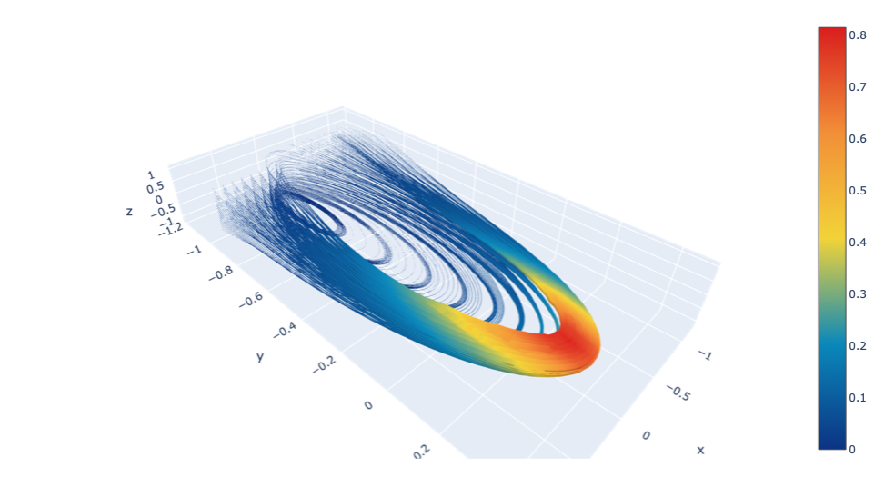
(a) $t=0$

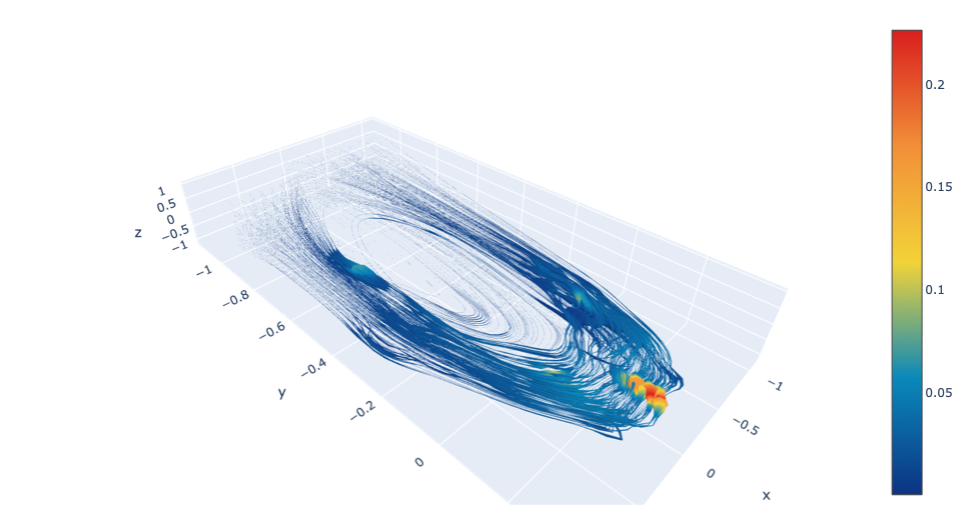
(b) $t=0.1$

(c) $t=0.2$

Figure 7.1: Computed streamlines of the flow flow at $t=0$, $0.1$, $0.2$ in the first experiment.

In the first simulation (cf. Fig. 7.1) the initial data are chosen as

$$(X_{0}^{1},\omega_{0}^{1})=((0,0,0),(0,0,0.1)),\quad(X_{0}^{2},\omega_{0}^{2})=((0,1,0),(0,0,-0.1))$$

and

$$(X_{0}^{3},\omega_{0}^{3})=((0,0,1),(0,0.1,0)),$$

each with 100 independent copies. Because of the diffusion, additional swirling eddies appear in the flow, and the magnitude of the velocity is diffused into the whole flow.

In the second simulation, we assess our numerical scheme by considering the known evolution of the Lamb–Oseen vortex, a line vortex that decays because of the presence of viscosity. Although the Lamb–Oseen vortex is typically regarded as a 2D solution with initial vorticity $\delta(x)\delta(y)$ for $(x,y)\in\mathbb{R}^{2}$, we consider it here as a 3D vortex solution with initial vorticity $(0,0,\delta(x)\delta(y))$ for $(x,y,z)\in\mathbb{R}^{3}$. Then, the exact solution of the resulting 3D Lamb–Oseen vortex evolution problem, with $\nu=\frac{1}{2}$, is given by

$$u(x,y,z,t)=\frac{1}{2\pi}\frac{(-y,x,0)}{x^{2}+y^{2}}(1-\mathrm{e}^{-\frac{x^{2}+y^{2}}{2t}}),\qquad(x,y,z)\in\mathbb{R}^{3},\;t>0.$$ (7.5)

In our numerical simulations the evolution of the computed solution is initialized at $x_{k}=(0,0,k/2)$ with $\omega_{k}=(0,0,1/2)$ for $-20\leq k\leq 20$, and we consider the velocity field projected on the plane $z=0$ when $t=0.1$ (cf. Fig. 7.2). It is clear from the figures that the resemblance between the exact velocity field depicted in Fig. 7.2 (a) and the computed velocity field with $N=1$, $20$ and $100$ independent copies, shown in Fig. 7.2 (b), (c), (d), respectively, improves as $N$ increases. To compare the computed velocity fields with the exact velocity field more precisely, a lattice consisting of 25 points in the horizontal plane, $z=0$, was chosen; the values at these points of the exact and approximate velocity fields projected on the plane $z=0$ are shown in Table 7.1. In addition, we have calculated the error between the exact solution and the approximate solution in the discrete counterpart of the $L^{1}_{[0,1]^{3}}$ norm. More precisely, we sum $|u_{\text{approx}}-u_{\text{exact}}|$ over the lattice $(\frac{i}{10},\frac{j}{10},\frac{k}{10})_{-10\leq i,j,k\leq 9}$ and then multiply the resulting sum by $0.1^{3}$, where $u_{\text{approx}}$ is the velocity field calculated using our scheme, while $u_{\text{exact}}$ is the exact velocity field. In Table 7.1, only the first two coordinates of the 25 lattice points and the first two components of the three-component vectors of the exact and approximate velocity fields at the 25 lattice points are shown. The third component of the exact velocity field is identically $0$; for the values of the approximate velocity fields at the lattice points, listed in the third, fourth and fifth columns of the table, the third component is not exactly $0$, but was in all cases less than $10^{-4}$.

We apply the numerical scheme, slightly modified, instead of (6.3) and (6.5). More precisely we use the following scheme:

$$\mathrm{d}X_{t}^{(\boldsymbol{i},\rho),i}=\frac{h^{3}}{N}\sum_{\boldsymbol{k}\neq\boldsymbol{i}}\omega_{\boldsymbol{k}}^{\beta}\sum_{\sigma=1}^{N}\left[K_{\alpha}^{i}(X_{t}^{(\boldsymbol{i},\rho)}-X_{t}^{(\boldsymbol{k},\sigma)})\,G_{\beta}^{(\boldsymbol{k},\sigma),\alpha}(t,0)\right]\!\mathrm{d}t+\sqrt{2\nu}\,\mathrm{d}B_{t}^{i,\rho},$$ (7.6)

$$\frac{\mathrm{d}}{\mathrm{d}s}G_{j}^{(\boldsymbol{l},\lambda),i}(t,s)\!=\!-\frac{h^{3}}{N}\,G_{l}^{(\boldsymbol{l},\lambda),i}(t,s)\!\sum_{\boldsymbol{k}\neq\boldsymbol{l}}\omega_{\boldsymbol{k}}^{\beta}\sum_{\sigma=1}^{N}\!\left[H_{j,\alpha}^{l}(X_{s}^{(\boldsymbol{l},\lambda)}-X_{s}^{(\boldsymbol{k},\sigma)})\,G_{\beta}^{(\boldsymbol{k},\sigma),\alpha}(s,0)\right].$$ (7.7)

There are $N\rho$ independent Brownian motions instead of $\rho$ independent Brownian motions for the whole system and $X^{i,\rho}$ are driven by independent Brownian motions. A numerical algorithm is developed based on this system by time discretization. The numerical experiment with this scheme helps avoid using a large number of copies but still gives a stable result. This scheme however reduces the computational costs.

The scheme is tested for the Taylor–Green vortex with the Reynolds number set to 1600. The initial velocity has components $\cos(x)\sin(y)\sin(z)$, $-\sin(x)\cos(y)\sin(z)$ and $0$. The simulation is initialized with the lattice points $(\frac{\pi}{16}i,\frac{\pi}{16}j,\frac{\pi}{16}k)_{-16\leq i,j,k\leq 48}$, and $N=1$. We compare the evolution of the velocity field projected on the plane $z=0.1$. We see that the simulation results resemble the real solution quite well (cf. Fig. 7.3). In order to explore the improvement resulting from reduction of the step size, we conducted another simulation with the same initialization but with step size $\Delta t=0.01$ instead of $0.02$ (cf. Fig. 7.3). In Table 7.2, a lattice consisting of 25 points on this plane was chosen, and the values at these points of the exact and approximate velocity fields projected on the plane $z=0.1$ are shown. In addition, we have calculated the $L^{1}_{[\frac{\pi}{2},\frac{3\pi}{2}]^{2}}$ norm error between the exact solution and the approximate solutions. It is clear that the accuracy of the approximation is improved by reducing the step size $\Delta t$.

Next, the scheme is tested in the case of artificial homogeneous isotropic turbulence. The turbulence is initiated by a solenoidal velocity field

$$u(x,y,z)=( \cos(x)\sin(y)\sin(z)+\cos(x)\sin(y)\sin(2z),$$ (7.8)

$$-\sin(x)\cos(y)\sin(z)+\sin(x)\cos(y)\sin(2z),$$

$$-\sin(x)\sin(y)\cos(2z)).$$

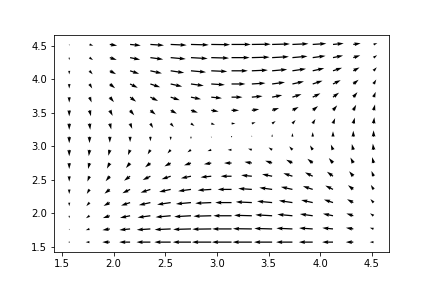
(a)

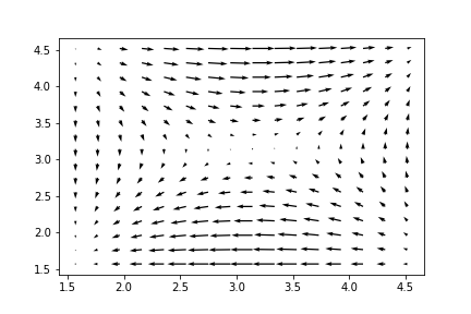
(b)

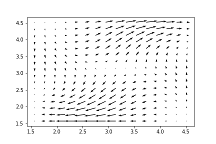
(c)

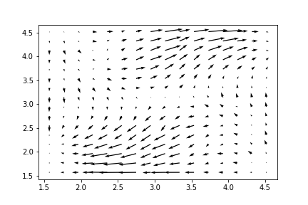
(d)

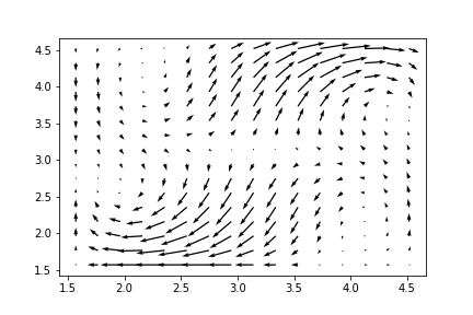
(e)

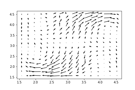
(f)

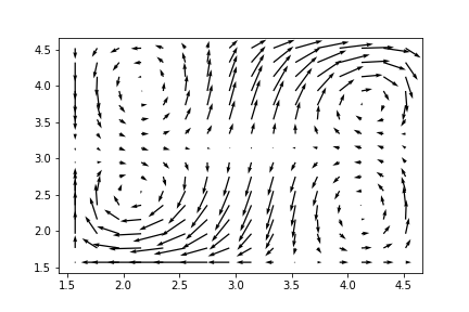
(g)

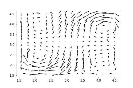
(h)

Figure 7.4: The images in the left column represent the DNS solution. Those in the right column have been obtained using the proposed scheme; from the top to the bottom, $t=0,0.3,0.6,1$, respectively.

We compare our numerical results with the results obtained by DNS. The DNS is based on a pseudo-spectral Fourier–Galerkin method [11]. The code for the implementation of DNS is based on the algorithm suggested in [44, 40]. The Reynolds number is 1600 as in the numerical verification in [40], so that the viscosity $\nu$ is $\frac{1}{1600}$, accordingly. The simulation is initialized using the lattice points $(\frac{\pi}{16}i,\frac{\pi}{16}j,\frac{\pi}{16}k)_{-16\leq i,j,k\leq 48}$ and $N=1$. We compare the evolution of the velocity field projected onto the plane $z=0.1$. The simulation and the DNS solution produce very similar results (cf. Fig. 7.4).

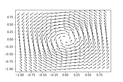
(a)

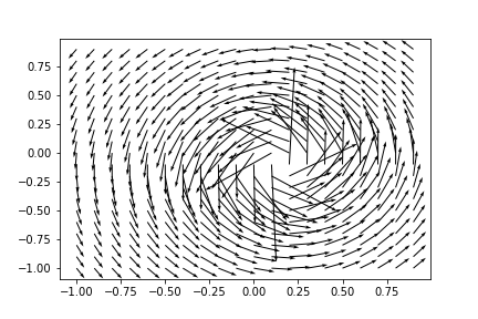
(b)

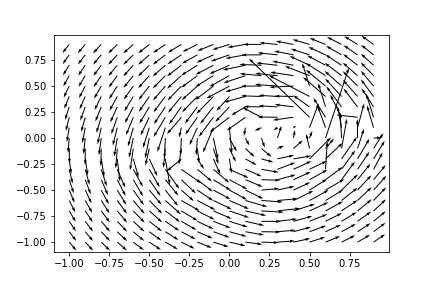
(c)

(d)

Figure 7.2: The velocity field of the Lamb–Oseen vortex at $t=0.1$: (a) the exact solution; and the numerical solution computed with, respectively, (b) $N=1$, (c) $N=20$, (d) $N=100$ independent copies.

Point	Exact value	$N=1$	$N=20$	$N=100$
($-1.0$, $-1.0$)	($0.08$, $-0.08$)	($0.06$,$-0.08$)	($0.06$,$-0.08$)	($0.08$, $-0.08$)
($-0.5$, $-1.0$)	($0.13$, $-0.06$)	($0.11$, $-0.08$)	($0.10$, $-0.07$)	($0.13$, $-0.07$)
($0.0$, $-1.0$)	($0.16$, $0.00$)	($0.17$, $-0.03$)	($0.14$, $-0.03$)	($0.15$, $0.01$)
($0.50$, $-1.0$)	($0.13$, $0.06$)	($0.15$, $0.06$)	($0.14$, $0.04$)	($0.12$, $0.07$)
($1.00$, $-1.0$)	($0.08$, $0.08$)	($0.09$, $0.08$)	($0.10$, $0.07$)	($0.08$, $0.08$)
($-1.0$, $-0.5$)	($0.06$, $-0.13$)	($0.04$, $-0.12$)	(0.05, $-0.11$)	($0.05$, $-0.13$)
($-0.5$, $-0.5$)	($0.15$, $-0.15$)	($0.11$, $-0.17$)	($0.11$, $-0.13$)	($0.11$, $-0.14$)
($0.0$, $-0.5$)	($0.23$, $0.00$)	($0.30$, $-0.16$)	($0.16$, $-0.09$)	($0.17$, $0.01$)
($0.5$, $-0.5$)	($0.15$, $0.15$)	($0.21$, $0.18$)	($0.16$, $0.10$)	($0.13$, $0.14$)
($1.0$, $-0.5$)	($0.06$, $0.13$)	($0.07$, $0.15$)	($0.10$, $0.13$)	($0.06$, $0.12$)
($-1.0$, $0.0$)	($-0.00$, $-0.16$)	($-0.01$, $-0.13$)	($-0.01$, $-0.13$)	($-0.02$, $-0.14$)
($-0.5$, $0.0$)	($-0.00$, $-0.23$)	($-0.04$, $-0.24$)	($-0.04$, $-0.18$)	($-0.04$, $-0.22$)
($0.0$, $0.0$)	($-0.00$, $0.00$)	($-0.26$, $-0.37$)	($0.06$, $-0.12$)	($-0.09$, $0.04$)
($0.5$, $0.0$)	($-0.00$, $0.23$)	($-0.18$, $0.32$)	($0.02$, $0.06$)	($0.02$, $0.21$)
($1.0$, $0.0$)	($-0.00$, $0.16$)	($-0.02$, $0.18$)	($-0.03$, $0.24$)	($0.00$, $0.15$)
($-1.0$, $0.5$)	($-0.06$, $-0.13$)	($-0.06$, $-0.10$)	($-0.05$, $-0.10$)	($-0.06$, $-0.11$)
($-0.5$, $0.5$)	($-0.15$, $-0.15$)	($-0.12$, $-0.13$)	($-0.10$, $-0.12$)	($-0.13$, $-0.13$)
($0.0$, $0.5$)	($-0.23$, $0.00$)	($-0.24$, $-0.07$)	($-0.21$, $-0.11$)	($-0.20$, $0.00$)
($0.5$, $0.5$)	($-0.15$, $0.15$)	($-0.19$, $0.11$)	($-0.06$, $0.20$)	($-0.13$, $0.12$)
($1.0$, $0.5$)	($-0.06$, $0.13$)	($-0.09$, $0.12$)	($-0.10$, $0.13$)	($-0.06$, $0.13$)
($-1.0$, $1.0$)	($-0.08$, $-0.08$)	($-0.07$, $-0.07$)	($-0.06$, $-0.07$)	($-0.07$, $-0.07$)
($-0.5$, $1.0$)	($-0.13$, $-0.06$)	($-0.10$, $-0.06$)	($-0.10$, $-0.07$)	($-0.11$, $-0.06$)
($0.0$, $1.0$)	($-0.16$, $0.00$)	($-0.14$, $-0.02$)	($-0.14$, $-0.04$)	($-0.14$, $-0.01$)
($0.5$, $1.0$)	($-0.13$, $0.06$)	($-0.13$, $0.04$)	($-0.14$, $0.04$)	($-0.13$, $0.05$)
($1.0$, $1.0$)	($-0.08$, $0.08$)	($-0.09$, $0.07$)	($-0.10$, $0.07$)	($-0.08$, $0.08$)
$L^{1}_{[-1,1]^{3}}$ norm error		Error $=0.91$	Error $=0.66$	Error $=0.19$

Table 7.1: The exact values of the velocity field in the Lamb–Oseen vortex problem at $t=0.1$ (second column) at 25 lattice points (first column), and the values of the computed velocity field at those points, with $N=1$ (third column), $N=20$ (fourth column), and $N=100$ (fifth column) independent copies, corresponding to the images depicted in Fig. 7.2. The discrete $L^{1}_{[-\frac{,}{1}]^{3}}$ norm error based on the $20^{3}$ lattice points $(\frac{i}{10},\frac{j}{10},\frac{k}{10})_{-10\leq i,j,k\leq 9}$ is shown in the last row of the table.

Point	Exact value	$\Delta t=0.02$	$\Delta t=0.01$
( $1.57$ , $1.57$)	( $-0.00$ , $-0.00$)	( $0.00$ , $-0.00$)	( $0.00$ , $-0.01$)
( $2.20$ , $1.57$)	( $0.05$ , $-0.00$)	( $0.04$ , $-0.00$)	( $0.03$ , $-0.01$)
( $2.83$ , $1.57$)	( $-0.04$ , $-0.00$)	( $-0.08$ , $-0.01$)	( $-0.07$ , $-0.01$)
( $3.46$ , $1.57$)	( $-0.17$ , $-0.00$)	( $-0.15$ , $-0.00$)	( $-0.18$ , $-0.01$)
( $4.08$ , $1.57$)	( $-0.17$ , $-0.00$)	( $-0.15$ , $-0.00$)	( $-0.17$ , $-0.00$)
( $1.57$ , $2.20$)	( $-0.00$ , $0.17$)	( $-0.00$ , $0.15$)	( $0.00$ , $0.17$)
( $2.20$ , $2.20$)	( $0.06$ , $0.15$)	( $0.06$ , $0.13$)	( $0.04$ , $0.15$)
( $2.83$ , $2.20$)	( $-0.02$ , $0.12$)	( $-0.13$ , $0.14$)	( $-0.04$ , $0.11$)
( $3.46$ , $2.20$)	( $-0.15$ , $0.09$)	( $-0.15$ , $0.08$)	( $-0.16$ , $0.08$)
( $4.08$ , $2.20$)	( $-0.15$ , $0.06$)	( $-0.14$ , $0.04$)	( $-0.15$ , $0.04$)
( $1.57$ , $2.83$)	( $-0.00$ , $0.17$)	( $-0.00$ , $0.11$)	( $0.00$ , $0.18$)
( $2.20$ , $2.83$)	( $0.09$ , $0.15$)	( $0.08$ , $0.13$)	( $0.08$ , $0.15$)
( $2.83$ , $2.83$)	( $0.04$ , $0.09$)	( $0.04$ , $0.08$)	( $0.02$ , $0.10$)
( $3.46$ , $2.83$)	( $-0.09$ , $0.04$)	( $-0.09$ , $0.03$)	( $-0.10$ , $0.03$)
( $4.08$ , $2.83$)	( $-0.12$ , $-0.02$)	( $-0.11$ , $-0.03$)	( $-0.12$ , $-0.04$)
( $1.57$ , $3.46$)	( $-0.00$ , $0.04$)	( $-0.00$ , $0.03$)	( $0.00$ , $0.07$)
( $2.20$ , $3.46$)	( $0.12$ , $0.02$)	( $0.12$ , $-0.01$)	( $0.12$ , $0.04$)
( $2.83$ , $3.46$)	( $0.09$ , $-0.04$)	( $0.11$ , $-0.03$)	( $0.09$ , $-0.02$)
( $3.46$ , $3.46$)	( $-0.04$ , $-0.09$)	( $-0.03$ , $-0.08$)	( $-0.03$ , $-0.09$)
( $4.08$ , $3.46$)	( $-0.09$ , $-0.15$)	( $-0.07$ , $-0.14$)	( $-0.08$ , $-0.15$)
( $1.57$ , $4.08$)	( $-0.00$ , $-0.05$)	( $-0.00$ , $-0.02$)	( $0.00$ , $-0.03$)
( $2.20$ , $4.08$)	( $0.15$ , $-0.06$)	( $0.14$ , $-0.05$)	( $0.15$ , $-0.04$)
( $2.83$ , $4.08$)	( $0.15$ , $-0.09$)	( $0.14$ , $-0.10$)	( $0.15$ , $-0.08$)
( $3.46$ , $4.08$)	( $0.02$ , $-0.12$)	( $0.05$ , $-0.11$)	( $0.04$ , $-0.12$)
( $4.08$ , $4.08$)	( $-0.06$ , $-0.15$)	( $-0.06$ , $-0.13$)	( $-0.04$ , $-0.15$)
$L^{1}_{[\frac{\pi}{2},\frac{3\pi}{2}]^{2}}$ norm error		Error $=0.26$	Error $=0.20$

Table 7.2: The exact values of the velocity field of the Taylor–Green vortex at $t=1$ (second column) at 25 lattice points (first column), and the values of the computed velocity field at those points, with $\Delta t=0.02$ (third column), $\Delta t=0.01$ (fourth column) corresponding to the images depicted in Fig. 7.3.

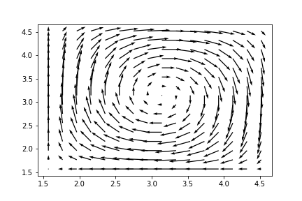
(a)

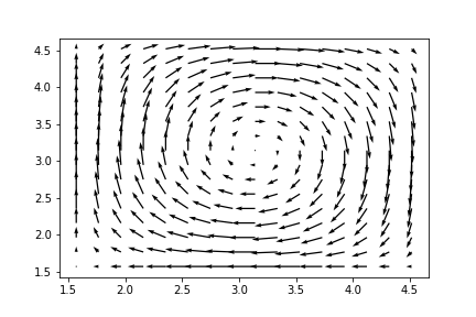
(b)

(c)

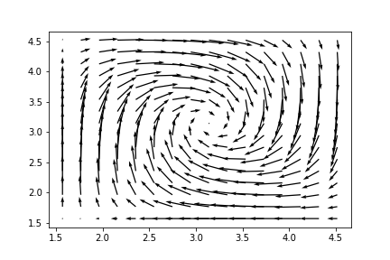
(d)

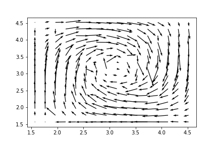
(e)

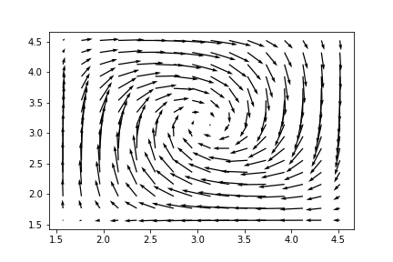
(f)

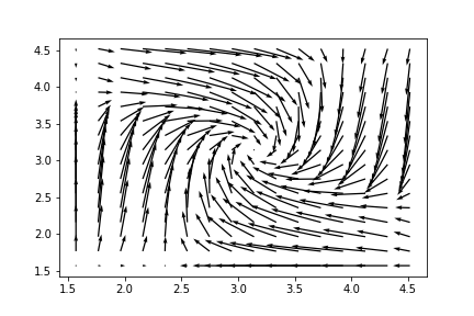
(g)

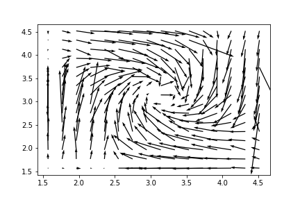
(h)

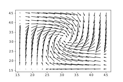
(i)

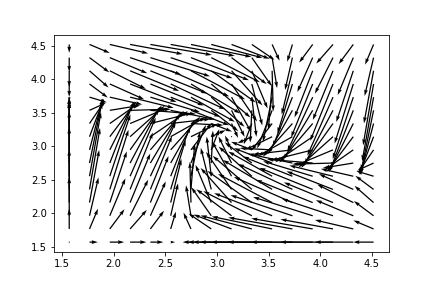
(j)

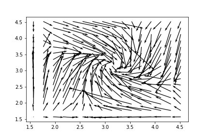
(k)

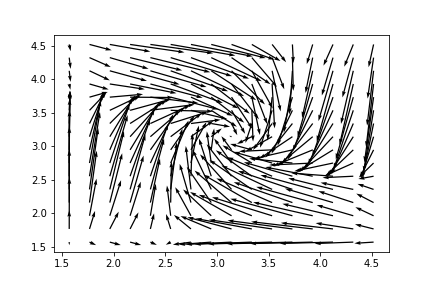
(l)

Figure 7.3: The images in the left column represent the Taylor–Green vortex solution. Those in the right column have been obtained using the proposed scheme. From the top to the bottom, $t=0,0.3,0.6,1$, respectively. The images in the left column represent the Taylor–Green vortex solution. Those in the middle column and right column have been obtained using the proposed scheme with step size $\Delta t=0.02$ and $0.01$, respectively; from the top to the bottom, $t=0,0.3,0.6,1$.

Data Accessibility

The code for the simulations is available on Dryad [49].

References

• [1] A. D. A. D. Venttsel’. On boundary conditions for multidimensional diffusion processes. Theory of Probability and Its Applications, 4(2):10.1137/1104014, 1959.
• [2] S. Albeverio and Y. Belopolskaya. Generalized solutions of the cauchy problem for the navier-stokes system and diffusion processes. CUBO, A Mathematical Journal, 12(2):77–96, 2010.
• [3] C. Anderson and C. Greengard. On vortex methods. SIAM Journal on Numerical Analysis, 22(3):413–440, 1985.
• [4] J. T. Beale. A convergent 3-d vortex method with grid-free stretching. Mathematics of Computation, 46(174):401–424, 1986.
• [5] J. T. Beale and A. Majda. Rates of convergence for viscous splitting of the Navier–Stokes equations. Mathematics of Computation, 37(156):243–259, 1981.
• [6] J. T. Beale and A. Majda. Vortex methods, I. Convergence in three dimensions. Mathematics of Computation, 39(159):1–27, 1982.
• [7] J. T. Beale and A. Majda. Vortex methods, II. Higher order accuracy in two and three dimensions. Mathematics of Computation, 39(159):29–52, 1982.
• [8] A. Beaudoin, S. Huberson, and E. Rivoalen. Simulation of anisotropic diffusion by means of a diffusion velocity method. Journal of Computational Physics, 186(1):122–135, 2003.
• [9] R. M. Blumenthal and R. K. Getoor. Markov processes and potential theory. Academic Press, 1986.
• [10] B. Busnello, F. Flandoli, and M. Romito. A probabilistic representation for the vorticity of a three-dimensional viscous fluid and for general systems of parabolic equations. Proceedings of the Edinburgh Mathematical Society, 48(2):295–336, 2005.
• [11] C. Canuto, M. Y. Hussaini, A. Quarteroni, and T. A. Zang Jr. Spectral methods in fluid dynamics. Springer, Berlin, Heidelberg, 1988.
• [12] A. J. Chorin. Numerical study of slightly viscous flow. Journal of Fluid Mechanics, 57(4):785–796, 1973.
• [13] A. J. Chorin. Vorticity and turbulence. Springer Science & Business Media, 1994.
• [14] A. J. Chorin and P. S. Bernard. Discretization of a vortex sheet, with an example of roll-up. Journal of Computational Physics, 13(3):423–429, 1973.
• [15] K. L. Chung and J. B. Walsh. Markov processes, Brownian motion, and time symmetry. Springer Science & Business Media, 2006.
• [16] P. Constantin and G. Iyer. A stochastic lagrangian representation of the three-dimensional incompressible navier-stokes equations. Communications on Pure and Applied Mathematics: A Journal Issued by the Courant Institute of Mathematical Sciences, 61(3):330–345, 2008.
• [17] G.-H. Cottet, J. Goodman, and T. Y. Hou. Convergence of the grid-free point vortex method for the three-dimensional Euler equations. SIAM Journal on Numerical Analysis, 28(2):291–307, 1991.
• [18] G.-H. Cottet and P. D. Koumoutsakos. Vortex methods: theory and practice. Cambridge University Press, Cambridge, 2000.
• [19] G.-H. Cottet and S. Mas-Gallic. A particle method to solve the Navier–Stokes system. Numerische Mathematik, 57(1):805–827, 1990.
• [20] P. Degond and S. Mas-Gallic. The weighted particle method for convection-diffusion equations, I. The case of an isotropic viscosity. Mathematics of Computation, 53(188):485–507, 1989.
• [21] C. Dellacherie and P. A. Meyer. Probabiliti$\acute{e}$s et potentiel, Chapitres XII $\grave{a}$ XVI. Hermann, 1987.
• [22] R. P. Feynman. Space-time approach to non-relativistic quantum mechanics. Feynman’s Thesis—A New Approach To Quantum Theory, pages 71–109, 2005.
• [23] A. Friedman. Partial differential equations of parabolic type. Prentice-Hall, INC., 1964.
• [24] J. Fronteau and P. Combis. A Lie-admissible method of integration of Fokker–Planck equations with non-linear coefficients (exact and numerical solutions). Technical report, CEA Centre d’Etudes Nucleaires de Saclay, 1984.
• [25] Y. Gao, J. Liang, and T.-J. Xiao. A new method to obtain uniform decay rates for multidimensional wave equations with nonlinear acoustic boundary conditions. SIAM Journal on Control and Optimization, 56(2):1303–1320, 2018.
• [26] Y. Gao and J.-M. Roquejoffre. Asymptotic stability for diffusion with dynamic boundary reaction from ginzburg-landau energy. arXiv 2201.02105, 2022.
• [27] M. Gazzola, B. Hejazialhosseini, and P. Koumoutsakos. Reinforcement learning and wavelet adapted vortex methods for simulations of self-propelled swimmers. SIAM Journal on Scientific Computing, 36(3):B622–B639, 2014.
• [28] J. Goodman. Convergence of the random vortex method. Communications on Pure and Applied Mathematics, 40(2):189–220, 1987.
• [29] J. Hale. Theory of functional differential equations. Springer-Verlag, 1977.
• [30] N. Ikeda and S. Watanabe. Stochastic differential equations and diffusion processes. North-Holland Pub. Company, 2nd edition edition, 1989.
• [31] M. Kac. On some connections between probability theory and differential and integral equations. In Proceedings of the second Berkeley symposium on mathematical statistics and probability, pages 189–215. University of California Press, 1951.
• [32] M. Kac. Probability and Related Topics in Physical Sciences. American Mathematical Soc., 1959.
• [33] O. M. Knio and A. F. Ghoniem. Numerical study of a three-dimensional vortex method. Journal of Computational Physics, 86(1):75–106, 1990.
• [34] J. N. Kutz. Deep learning in fluid dynamics. Journal of Fluid Mechanics, 814:1–4, 2017.
• [35] S. Lee and D. You. Data-driven prediction of unsteady flow over a circular cylinder using deep learning. Journal of Fluid Mechanics, 879:217–254, 2019.
• [36] D.-G. Long. Convergence of the random vortex method in two dimensions. Journal of the American Mathematical Society, 1(4):779–804, 1988.
• [37] T. Lyons and L. Stoica. The limits of stochastic integrals of differential forms. The Annals of Probability, 27(1):1–49, 1999.
• [38] T. Lyons and W. Zheng. A crossing estimate for the canonical process on a Dirichlet space and a tightness result. Astérisque, 157–158:249–271, 1988.
• [39] A. J. Majda and A. L. Bertozzi. Vorticity and incompressible flow. Cambridge University Press, 2002.
• [40] M. Mortensen and H. P. Langtangen. High performance python for direct numerical simulations of turbulent flows. Computer Physics Communications, 203:53–65, 2016.
• [41] J. Nash. Continuity of solutions of parabolic and elliptic equations. American Journal of Mathematics, 80(4):931–954, 1958.
• [42] Y. Ogami and T. Akamatsu. Viscous flow simulation using the discrete vortex model—the diffusion velocity method. Computers & Fluids, 19(3-4):433–441, 1991.
• [43] C. Olivera. Probabilistic representation for mild solution of the navier–stokes equations. Mathematical Research Letters, 28(2):563–573, 2021.
• [44] S. A. Orszag and G. Patterson Jr. Numerical simulation of three-dimensional homogeneous isotropic turbulence. Physical Review Letters, 28(2):76, 1972.
• [45] M. Ossiander. A probabilistic representation of solutions of the incompressible navier-stokes equations in r3. Probability theory and related fields, 133(2):267–298, 2005.
• [46] E. Pardoux and S. G. Peng. Adapted solution of a backward stochastic differential equation. Systems & Control Letters, 14(1):55–61, 1990.
• [47] S. G. Peng. Probabilistic interpretation for systems of quasilinear parabolic partial differential equations. Stochastics and Stochastics Reports (Print), 37(1-2):61–74, 1991.
• [48] Z. Qian, Y. Qiu, and Y. Zhang. Tracking the vortex motion by using Brownian fluid particles. Physics of Fluids, 33(10):105113, 2021.
• [49] Z. Qian, E. Süli, and Y. Zhang. The code of random vortex simulations. 2021. doi: 10.5061/dryad.44j0zpcgs.
• [50] L. Rosenhead. The point vortex approximation of a vortex sheet. Proc. Roy. Soc. London Ser. A, 134:170–192, 1932.
• [51] D. W. Stroock and S. R. S. Varadhan. Diffusion processes with boundary conditions. Commun. on Pure and Appl. Math., 24:147–225, 1971.
• [52] D. W. Stroock and S. S. Varadhan. Multidimensional diffusion processes. Springer, 1979.
• [53] G. I. Taylor. Diffusion by continuous movements. Proceedings of the London Mathematical Society, 2(1):196–212, 1922.
• [54] Z. Wang, J. Xin, and Z. Zhang. Sharp error estimates on a stochastic structure-preserving scheme in computing effective diffusivity of 3d chaotic flows. Multiscale Modeling & Simulation, 19(3):1167–1189, 2021.
• [55] X. Zhang. A stochastic representation for backward incompressible navier-stokes equations. Probability theory and related fields, 148(1):305–332, 2010.
• [56] X. Zhang. Stochastic differential equations with sobolev diffusion and singular drift and applications. The Annals of Applied Probability, 26(5):2697–2732, 2016.