Nuclear states projected from a pair condensate

Abstract

Atomic nuclei exhibit deformation, pairing correlations, and rotational symmetries. To meet these competing demands in a computationally tractable formalism, we revisit the use of general pair condensates with good particle number as a trial wave function for even-even nuclei. After minimizing the energy of the condensate, allowing for general triaxial deformations, we project out states with good angular momentum with a fast projection technique. To show applicability, we present example calculations from pair condensates in several model spaces, and compare against angular-momentum projected Hartree-Fock and full configuration-interaction shell model calculations. This approach successfully generates spherical, vibrational and rotational spectra, demonstrating potential for modeling medium- to heavy-mass nuclei.

I Introduction

Medium- and heavy-mass nuclides exhibit a rich portfolio of behaviors, not only the classic rotational, vibrational, and superfluid (spherical) spectra Bohr and Mottelson (1998); Ring and Shuck (1980), but also triaxial deformation and wobbling Frauendorf and Dönau (2014) and chiral doublet bands Ayangeakaa et al. (2013). An accurate description of the many-body wave functions of heavy nuclides is important to understanding alpha cluster pre-formation in $\alpha$-decay  Xu et al. (2017) as well as nucleosynthesis in astrophysical environments Surman et al. (2016); Kajino et al. (2019).

There are numerous microscopic approaches to modeling heavy nuclei, including the relativistic mean field method Meng (2016), the Hartree-Fock Bogoliubov method Ring and Shuck (1980); Bally and Bender (2021); Sánchez-Fernández et al. (2021); Bally et al. (2019); Shimizu et al. (2021), the random phase and related approximations Ring and Shuck (1980), and algebraic models (e.g. the Interacting Boson Model Iachello and Arima (2006)), as well as the projected shell model Sun et al. (2000) and powerful Monte Carlo methods Otsuka et al. (2001).

Here we focus on the configuration-interacting shell model, which has been successful in reproducing low-lying states and transition rates of light and medium-heavy nuclei Caurier et al. (2005); Brown (2001). Within a given valence space and with a good effective interactions, the configuration-interaction shell model reproduces large amounts of data. The downside of configuration-interaction methods, however, is they are at the mercy of the valence space. While any calculation in the $1s0d$ shell is nowadays nearly trivial  Brown and Richter (2006) and much of the $1p0f$ shell is accessible  Honma et al. (2002, 2005), as one reaches up to the $2s1d0g_{7/2}0h_{11/2}$ space (nuclides with $N,Z\in[50,82]$), calculations quickly become intractable due to the large dimension of the many-body basis.

Among many different configuration-interaction truncation schemes, one is to construct the basis from products of a restricted set of fermion pairs coupled to angular momentum $0,2,4,6,\cdots$ (S, D, G, I pairs). In low-lying states, such pairs are favored energetically. An example of this is the general seniority model, which focuses on S-pair condensates and their breaking Talmi (1993); Jia (2019, 2016, 2015), and is especially useful in semi-magic nuclei. Going further, the nucleon-pair approximation (NPA) truncates the configuration space with angular-momentum coupled fermion pairs, and has proved to be effective in medium-heavy and heavy nuclei with schematic pairing-plus-quadrupole-quadrupole interactions Zhao and Arima (2014); Higashiyama et al. (2002). In the NPA matrix elements and overlaps between many-pair states with good total angular momentum (i.e., $J$-scheme) are computed using commutation relations, which become numerically burdensome as the number of pairs increase, in practice limiting calculations to a maximum of about 8 valence pairs. To address this burden, $M$-scheme NPA codes have been developed recently, pushing the upper limit of valence particles in the NPA to $Z_{\mathrm{valence}},N_{\mathrm{valence}}\leq 12$ He et al. (2020); Lei et al. (2021).

An alternate is to replace fermion pairs by bosons. The Interacting Boson Model (IBM) Iachello and Arima (2006) typically starts from S- and D-bosons and constructs Lie group reduction chains, classifying nuclei into different group limits. There have been efforts to map shell model calculations to boson models or pair models  Otsuka et al. (1978); Johnson and Ginocchio (1994); Ginocchio and Johnson (1995). While bosons models have the advantage of simpler commutation relations than fermion pairs, rigorous mapping of fermion pairs into bosons is far from trivial.

Related to the challenge of mapping fermion pairs to bosons is the problem of choosing the structure of the fermion pairs. Pairs determined from the variational principle, either from varying pairs by direct conjugate gradient descent, or extracted from a deformed Hartree-Fock (i.e., single-particle variation) state, can produce good quality spectra and transitions of transitional and deformed nuclei Fu and Johnson (2020, 2021); Lei et al. (2020). In other words, it can be useful to combine a variational approach (for optimization) and pair truncations (for small dimension).

Variational methods start from a given trial wave function (or ansatz) and minimizes the expectation value of the given Hamiltonian. Hartree-Fock calculations use a Slater determinant, an antisymmetrized product of single-particle states, as the ansatz, and varies the single-particle states to minimize the energy. The Hartree-Fock-Bogoliubov scheme utilizes a quasi-particle (Bardeen-Cooper-Schrieffer or BCS) vacuum constructed from a canonical basis as the trial wave function, and the canonical basis as well as BCS occupancies are varied Ring and Shuck (1980). Slater determinants used in Hartree-Fock calculations have the advantage of fast evaluation of Hamiltonian matrix elements, while the HFB scheme benefits from inherent simplicity of the quasi-particle vacuum.

Exploration of ansätze is important and can lead to new approaches Mizusaki and Schuck (2021). In this paper we focus on a pair condensate ansatz, well known in quantum chemistry as “antisymmetrized geminal power” wave functions Coleman (1965),

$$(\hat{A}^{\dagger})^{n}|0\rangle,~{}~{}~{}~{}\hat{A}^{\dagger}=\frac{1}{2}\sum_{\alpha\beta}A_{\alpha\beta}\hat{c}^{\dagger}_{\alpha}\hat{c}^{\dagger}_{\beta},$$ (1)

where $|0\rangle$ is the bare fermion vacuum, and $\hat{c}^{\dagger}_{\alpha},\hat{c}^{\dagger}_{\beta}$ are fermion creation operators with $\alpha,\beta$ labelling single-particle states (i.e. $\alpha$ stands for $(n_{\alpha}l_{\alpha}j_{\alpha}m_{\alpha})$), and, finally, $A_{\alpha\beta}$ are the “pair structure coefficients.” This is also called a “collective” pair, although sometimes that term is restricted to pairs with good angular momentum; we make no such restriction here. When we find a variational minimum, we restrict ourselves to real pair structure coefficients with skew symmetry $A_{\alpha\beta}=-A_{\beta\alpha}$; however later under rotation we will have complex skew-symmetric structure coefficients. With proper choice of $A_{\alpha\beta}$, such a condensate wave can be a Slater determinant as in Hartree-Fock theory Ring and Shuck (1980); Fu and Johnson (2020), or a seniority-0 state in Talmi’s generalized seniority model Talmi (1993), or particle-number-projected component of a BCS or HFB vacuum with particle number $2n$ Rowe et al. (1991). Therefore the pair condensate is a more general ansatz than any one of those limits.

The pair condensate ansatz has not been widely used in nuclear structure theory, however, because the evaluation of Hamiltonian matrix elements to be varied can be complicated Rowe et al. (1991); Chen et al. (1995); Lei et al. (2020), and the angular-momentum projection from a pair condensate has not been previously implemented for nuclear structure. In recent work Lei et al. (2021), we rederived formulas (see Johnson and Ginocchio (1994); Ginocchio and Johnson (1995) and references therein) for general $M$-scheme nucleon-pair bases,

$$\hat{A}^{\dagger}_{1}\cdots\hat{A}^{\dagger}_{n}|0\rangle,$$ (2)

with the pair condensate (1) as a special case. In this work we present the explicit formulas for pair condensates, and implement angular momentum projection after variation. Variation after angular momentum projection (VAP) leads to lower energies but are more complicated and time-consuming; hence we restrict ourselves to projection after variation (PAV). Hereafter, we label this approach as “projection after variation of a pair condensate” (PVPC). It is straightforward to introduce more pair condensates into the configuration space, such as in the generator coordinate method Ring and Shuck (1980), but for now we only consider one pair condensate.

In Sec. II, we outline the formalism for variation of a pair condensate, with details in the appendix. We show typical timing to find the minimum, as variation is the most time consuming part of the calculation, as exemplified by the descent of ¹³²Dy in the $2s1d0g_{7/2}0h_{11/2}$ shell. In Sec. II.1, we briefly introduce the formalism for angular momentum projection, following a recently developed recipe: linear algebraic projection (LAP) Johnson and O’Mara (2017); Johnson and Jiao (2019). In Sec. II.2, we decompose a pair condensate into fractions with good angular momentum, and show typical probability distributions for rotational nuclei and spherical nuclei. In Sec. II.3, we outline the fomalism for electromagnetic transitions between projected wavefunctions. In Sec. III, we present benchmark calculations of nuclides in the $1s0d,1p0f$ and $2s1d0g_{7/2}0h_{11/2}$ valence spaces with discussions and analysis. Finally we summarize and discuss future directions in Sec. IV.

II Formalism

For the nuclear many-body Hamiltonian, we use shell model effective interactions in occupation space, with 1- and 2-body parts, in proton-neutron format,

$$\hat{H}= \hat{H}_{0}+\hat{H}_{pp}+\hat{H}_{nn}+\hat{H}_{pn}$$ (3)

$$=\sum_{a\in\pi}\epsilon_{a}\hat{n}_{a}+\sum_{a\in\nu}\epsilon_{a}\hat{n}_{a}$$

$$+\sum_{abcd\in\pi}\frac{\sqrt{(1+\delta_{ab})(1+\delta_{cd})}}{4}\sum_{I}V_{pp}(abcd;I)\sum_{M}\hat{A}^{\dagger}_{IM}(ab)\hat{A}_{IM}(cd)$$

$$+\sum_{abcd\in\nu}\frac{\sqrt{(1+\delta_{ab})(1+\delta_{cd})}}{4}\sum_{I}V_{nn}(abcd;I)\sum_{M}\hat{A}^{\dagger}_{IM}(ab)\hat{A}_{IM}(cd)$$

$$+\sum_{ac\in\pi,bd\in\nu,I}V_{pn}(abcd;I)\sum_{M}\hat{A}^{\dagger}_{IM}(ab)\hat{A}_{IM}(cd).$$

where $\hat{A}^{\dagger}_{IM}(ab)$ and $\hat{A}_{IM}(cd)$ are so-called “non-collective” pair creations and annihilation operators (in contrast to the collective pair creation operator of Eq. (1)): $\hat{A}^{\dagger}_{IM}(ab)=\left[\hat{c}^{\dagger}_{a}\otimes\hat{c}^{\dagger}_{b}\right]_{IM},$ where $\otimes$ signals coupling via Clebsch-Gordan coefficients, and $\hat{A}_{IM}(ab)=\left(\hat{A}^{\dagger}_{IM}(ab)\right)^{\dagger}$.

We work in several model spaces: in the $1s_{1/2}$-$0d_{3/2}$-$0d_{5/2}$ or $1s0d$ shell, using the universal $1s0d$-shell interaction version B, or USDB   Brown and Richter (2006); in the $1p_{1/2}$-$1p_{3/2}$-$0f_{5/2}$-$0f_{7/2}$ or $1p0f$ shell, using a monopole-modified $G$-matrix interaction version 1A, or GX1A Honma et al. (2002, 2005); and finally, for the space between magic numbers 50 and 82, comprising the orbits $2s_{1/2}$-$1d_{3/2}$-$1d_{5/2}$-$0g_{7/2}$-$0h_{11/2}$, or $2s1d0g_{7/2}0h_{11/2}$, with a monopole-modified $G$-matrix interaction Qi and Xu (2012).

In order to carry out our calculations, we need a variety of matrix elements. To begin with, for variation (before projection) we need for a given state $|\Phi\rangle$: the normalization $\langle\Phi|\Phi\rangle$; the expectation value of a Hamiltonian or the energy of that state $E(\Phi)=\langle\Phi|\hat{H}|\Phi\rangle/\langle\Phi|\Phi\rangle$; and the variation of the energy with respect to some parameter $\partial E(\Phi)/\partial\lambda$. To carry out projection, we need the overlap or norm kernel of the state $\Phi$ with a rotated state $\Phi^{\prime}$, $\langle\Phi|\Phi^{\prime}\rangle$, the Hamiltonian matrix element or Hamiltonian kernel between these two states, $\langle\Phi|\hat{H}|\Phi^{\prime}\rangle$, and, finally, in order to calculate electromagnetic and other transitions represented by a one-body operators $\hat{Q}$, we need $\langle\Phi|\hat{Q}|\Phi^{\prime}\rangle$.

All of these are easily found for, say, Hartree-Fock and Hartree-Fock-Bogoliubov calculations. For the pair condensate calculations the formalism is more complicated and less intuitive. We present the detailed formalism in the Appendix, but sketch out the application here.

Restricting ourselves to even-even nuclei, our trial ansatz is a direct product of proton and neutron pair condensates

$$|\Phi\rangle=(\hat{A}^{\dagger}_{\pi})^{N_{\pi}/2}(\hat{A}^{\dagger}_{\nu})^{N_{\nu}/2}|0\rangle,$$ (4)

where $N_{\pi},N_{\nu}$ are valence numbers for protons and neutrons. We vary $|\Phi\rangle$, or more exactly, vary the proton and neutron pair structure coefficients, to minimize the energy

$$\frac{\langle\Phi|\hat{H}|\Phi\rangle}{\langle\Phi|\Phi\rangle}.$$ (5)

In order to find minima, we apply GNU scientific library (GSL) Galassi et al. (2019) conjugate gradient tools. We do variation before projection, that is, we first find the minimum energy of the unprojected pair condensate, and afterwards project out states of good angular momentum.

Fig. 1(a) shows the central processing unit (CPU) time for one iteration for $N=Z$ nuclei in different major shells, with increasing valence particles. Our timing data were taken on a $44$-core workstation using OpenMP parallelization. In the $1s0d,1p0f,2s1d0g_{7/2}0h_{11/2}$ major shells, the numbers of free parameters in variation of one pair condensate basis are $132,380,$ and $992$, respectively. The computation complexity of variation has polynomial dependence on the valence particle numbers. In Fig. 1 (b), an example is given for variation of ${}^{132}\mathrm{Dy}$ in the $2s1d0g_{7/2}0h_{11/2}$ shell, with interactions based on the CD-Bonn potential with the G matrix approach and monopole optimizations Qi and Xu (2012). With 992 free parameters, the iteration tends to converge after 200 steps. We note that the descent is steep for the first 50 steps, and less so afterwards. The descent terminates when the modulus of the gradient vector is smaller than a given criterion. If we set a stricter criterion on the gradient, the descent will continue beyond 200 steps, but with only a slight additional lowering of the energy. Starting from several independent random pairs, we typically find 2 or 3 local minima.

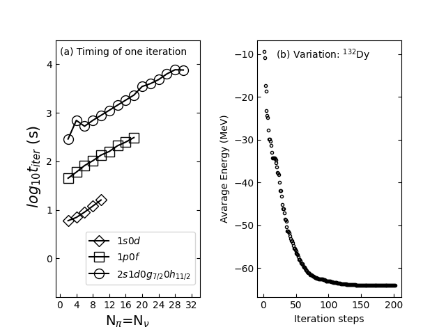
Figure 1: Panel (a): Logarithm CPU time (s) of one iteration in the variation for $N=Z$ nuclei, using conjugate gradient methodFletcher (1984) wrapped in the GNU Scientific Library function $\it gsl\_multimin\_fdf\_minimizer$Galassi et al. (2019). $1s0d$, $1p0f$, $2s1d0g_{7/2}0h_{11/2}$ are three valence shells. All these data are collected on a 44-core small workstation, in parallel with simple OpenMP. Panel (b): The descent of the average energy $\langle\Phi|\hat{H}|\Phi\rangle/\langle\Phi|\Phi\rangle$ for ¹³²Dy as a test case in $2s1d0g_{7/2}0h{11/2}$ shell. There are $32(32-1)=992$ free parameters for the variation of the proton and neutron pairs.

II.1 Angular momentum projection

In this work we allow for triaxial deformations. While there is extensive literature on the standard quadrature approach for angular momentum projection Ring and Shuck (1980); Sun (2016); Yao et al. (2010); Rodríguez-Guzmán et al. (2002), we adopt the recently developed “linear algebraic projection”(LAP) technique  Johnson and O’Mara (2017); Johnson and Jiao (2019). Although both approaches are based on standard quantum theory of angular momentum Edmonds (1957), i.e. rotational properties of irreducible tensors, for our application we found LAP to be 10 times faster than quadrature.

For the standard development of angular momentum projection see Edmonds (1957); Ring and Shuck (1980). The basic idea is that a pair condensate state, or any state $|\Phi\rangle$ for that matter, can be decomposed with normalized spherical tensor components, with total angular momentum $I$ and angular momentum projection on the 3rd axis $K$,

$$|\Phi\rangle=\sum_{IK}c_{IK}|IK\rangle.$$ (6)

In any finite space the sums are not infinite but restricted to a maximum $I$, $K$, and in practice the coefficients $c_{IK}$ restricts the sum even further Johnson and O’Mara (2017). The projection operator $\hat{P}^{J}_{MK}$ picks out the $(J,K)$ spherical tensor component and rotates it to a $(J,M)$ spherical tensor,

$$\hat{P}^{J}_{MK}|\Phi\rangle=c_{JK}|J,K\rightarrow M\rangle.$$ (7)

Then one diagonalizes the Hamiltonian in the truncated space of

$$\left\{\hat{P}^{J}_{M,-J}|\Phi\rangle,~{}~{}\hat{P}^{J}_{M,-J+1}|\Phi\rangle,~{}~{}\cdots,~{}~{}\hat{P}^{J}_{M,J}|\Phi\rangle\right\}$$ (8)

Because the Hamiltonian is a scalar operator, thus commuting with the projection operator, and because $(\hat{P}^{J}_{MK})^{\dagger}=\hat{P}^{J}_{KM}$, $\hat{P}^{J}_{K^{\prime}M}\hat{P}^{J}_{MK}=\hat{P}^{J}_{K^{\prime}K}$, we only need

$$\langle\Phi|\hat{H}\hat{P}^{J}_{MK}|\Phi\rangle\equiv{\mathcal{H}}^{J}_{MK},$$ (9)

$$\langle\Phi|\hat{P}^{J}_{MK}|\Phi\rangle\equiv{\mathcal{N}}^{J}_{MK}.$$ (10)

We then solve a generalized eigenvalues problem, i.e., the Hill-Wheeler equation,

$$\sum_{K}{\mathcal{H}}^{J}_{K^{\prime}K}g^{r}_{JK}=\epsilon_{r,J}\sum_{K}{\mathcal{N}}^{J}_{K^{\prime}K}g^{r}_{JK}.$$ (11)

where $r$ denotes different states with angular momentum $J$, at most $2J+1$ states, and $g^{r}_{JK}$ values determine the projected wavefunction.

To project out states, either by quadrature or by LAP, one needs to rotate states about the Euler angles $\alpha,\beta,\gamma$, using the rotation operator

$$\hat{R}(\alpha,\beta,\gamma)=\exp\left(\frac{i\gamma}{\hbar}\hat{J}_{z}\right)\exp\left(\frac{i\beta}{\hbar}\hat{J}_{y}\right)\exp\left(\frac{i\alpha}{\hbar}\hat{J}_{z}\right).$$ (12)

The matrix elements of the rotation operator between spherical tensors, that is, states with good total angular momentum $j$ and $z$-component $m$, is the Wigner-$D$ matrix Edmonds (1957), $\langle j^{\prime}m^{\prime}|\hat{R}(\alpha,\beta,\gamma)|jm\rangle=\delta_{j^{\prime}j}D^{j}_{m^{\prime}m}(\alpha\beta\gamma).$

For a given set of Euler angles $\Omega=(\alpha,\beta,\gamma)$, the matrix element of rotational operator $\hat{R}(\Omega)$ is

$$\langle\Phi|\hat{R}(\Omega)|\Phi\rangle=\sum_{IMK}c^{*}_{IK}c_{IM}D^{I}_{KM}(\Omega)\langle IK|IM\rightarrow K\rangle=\sum_{IMK}D^{I}_{KM}(\Omega)\mathcal{N}^{I}_{KM}.$$ (13)

For a series of Euler angles $\Omega_{1},\Omega_{2},\cdots$, we calculate the norm kernels $\langle\Phi|\hat{R}(\Omega_{i})|\Phi\rangle$, as well as the $D$ functions $D^{I}_{KM}(\Omega_{i})$, and then find $\mathcal{N}^{I}_{KM}$ as solutions to a set of linear equations. Similarly the Hamiltonian kernel $\mathcal{H}^{I}_{KM}$ can be also found.

Traditional projection procedure relies on the orthogonality of the Wigner-$D$ functions and thus upon quadrature; therefore the more abscissas ( Euler angles) one takes, the more accurate the projected energies. The basis for LAP, Eq. (13) is exact, but in practice one truncates the sum over $I$ with $I\leq J_{max}$. To find $J_{max}$, one computes $f_{J}$, the fraction of $J$-components defined in (21), with $f_{J}=\sum_{M}|c_{JM}|^{2}$, and sets $J_{max}$ such that $f_{J}\geq f_{tol}$ for all $J\leq J_{max}$. We follow Johnson and Jiao (2019) and take $f_{tol}\sim 10^{-4}$ typically. The error in projection is due to this truncation. As a result of finite $J_{max}$, in LAP the number of Euler angles is smaller. We implemented both methods, and found that LAP is more than 10 times faster than quadrature, with same accuracy of the energies of low-lying states.

To carry out this projection we need to be able to rotate pair condensates. This is almost as straightforward as for Slater determinants in angular-momentum projected Hartree-Fock Johnson and O’Mara (2017): one simply rotates the single-particle states, defining the matrix element of the rotation operator on single-particle bases $\alpha,\beta$ as

$$\mathcal{D}_{\alpha\beta}(\Omega)=\langle n_{\alpha}l_{\alpha}j_{\alpha}m_{\alpha}|\hat{R}(\Omega)|n_{\beta}l_{\beta}j_{\beta}m_{\beta}\rangle=\delta_{n_{\alpha}n_{\beta}}\delta_{l_{\alpha}l_{\beta}}\delta_{j_{\alpha}j_{\beta}}D^{j_{\alpha}}_{m_{\alpha}m_{\beta}}(\Omega).$$ (14)

Under rotation, a nucleon-pair (1) then becomes

$$\hat{R}(\Omega)\hat{A}^{\dagger}=\frac{1}{2}\sum_{\alpha\beta\gamma\delta}A_{\alpha\beta}\mathcal{D}_{\gamma\alpha}(\Omega)\mathcal{D}_{\delta\beta}(\Omega)\hat{c}_{\gamma}^{\dagger}\hat{c}_{\delta}^{\dagger}=\frac{1}{2}\sum_{\gamma\delta}{A^{\prime}}_{\gamma\delta}\hat{c}_{\gamma}^{\dagger}\hat{c}^{\dagger}_{\delta}\equiv\hat{A^{\prime}}^{\dagger},$$ (15)

with new pair coefficients

$$A^{\prime}_{\gamma\delta}=\sum_{\alpha\beta}A_{\alpha\beta}\mathcal{D}_{\gamma\alpha}(\Omega)\mathcal{D}_{\delta\beta}(\Omega)=(\mathcal{D}(\Omega)A\mathcal{D}(\Omega)^{\top})_{\gamma\delta}.$$ (16)

Therefore, the matrix element of rotational operator $\hat{R}(\Omega)$ on a pair condensate is

$$\langle\hat{A}^{n}|\hat{R}(\Omega)|(\hat{A}^{\dagger})^{n}\rangle=\langle\hat{A}^{n}|(\hat{A^{\prime}}^{\dagger})^{n}|0\rangle,~{}~{}~{}A^{\prime}=\mathcal{D}(\Omega)A\mathcal{D}(\Omega)^{\top},$$ (17)

and similarly

$$\langle\hat{A}^{n}|\hat{H}\hat{R}(\Omega)|(\hat{A}^{\dagger})^{n}\rangle=\langle\hat{A}^{n}|\hat{H}(\hat{A^{\prime}}^{\dagger})^{n}|0\rangle,~{}~{}~{}A^{\prime}=\mathcal{D}(\Omega)A\mathcal{D}(\Omega)^{\top}.$$ (18)

Parity projection is similar and straightforward, with a given wavefunction $|\Psi\rangle$, the positive and negative parity components are ($\hat{\mathcal{P}}$ is the space inversion operator)

$$\frac{1}{2}(1\pm\hat{\mathcal{P}})|\Psi\rangle.$$ (19)

To invert a many-body wavefunction, is equivalent to inverting all its single particle orbits. When a pair is operated on by the space inversion operator, an additional phase factor is generated for the pair structure coefficients,

$$\hat{\mathcal{P}}\hat{A}^{\dagger}=\frac{1}{2}\sum_{\alpha\beta}A_{\alpha\beta}(\hat{\mathcal{P}}\hat{c}^{\dagger}_{\alpha})(\hat{\mathcal{P}}\hat{c}^{\dagger}_{\beta})=\frac{1}{2}\sum_{\alpha\beta}A_{\alpha\beta}(-1)^{l_{\alpha}+l_{\beta}}\hat{c}^{\dagger}_{\alpha}\hat{c}^{\dagger}_{\beta}.$$ (20)

In this work, we do both angular momentum and parity projections for the results in $2s1d0g_{7/2}0h_{11/2}$ shell.

II.2 Tensor decomposition of a pair condensate

As expressed by Eq. (6), a pair condensate can be decomposed into components with different angular momentum quantum numbers $(J,M)$. In other words, an optimized pair condensate is considered as a mixture of low-lying nuclear states. We define the fraction of probability $f_{J}$ for total angular momentum $J$ in a pair condensate, as in Sheikh et al. (2002),

$$f_{J}=\sum_{M}|c_{JM}|^{2},$$ (21)

where $c_{JM}$ is the amplitude of $(J,M)$ tensor component in the pair condensate, as in Eq. (6). To illustrate the decompositions for rotational and spherical nuclei, we show ⁵²Fe and ⁴⁸Ca, respectively, in Fig. 2. For ⁵²Fe, in Fig. 2(a) the decomposition is distributed across $J=0,2,4,6$ as expected for rotational nuclei. Conversely, for ⁴⁸Ca in Fig. 2(b), the wave function is almost entirely contained in the $J=0$ component; while there are non-zero $f_{J}$ for $J>0$ values, the magnitudes are too small to be seen in Fig. 2(b). Therefore the optimized condensate for semi-magic nuclei is mostly the spherical $J=0$ ground state, while tiny non-spherical components of the condensate are projected out to be the non-zero spectrum, which turn out to be surprisingly accurate in comparison with shell model results, as will be shown in Fig. 5.

However, if cranking, or variation with constraints, is involved, one can increase the fraction of components with higher $J$. As in the usual procedure  Ring and Shuck (1980), one optimizes the trial wave function using the effective Hamiltonian

$$\hat{H^{\prime}}=\hat{H}-\omega\langle J_{x}\rangle.$$ (22)

Fig. 2(c) shows the decomposition of ⁴⁸Ca at $\omega=0$ and $\omega=0.5$ MeV; the latter increases the components with $J>0$. Nonetheless for simplicity we restrict ourselves to optimization without cranking for the rest of this paper.

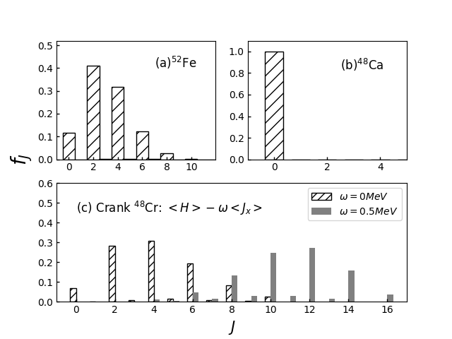
Figure 2: (a) Fractions of $J$-components in the optimized pair condensate for ⁵²Fe, as an example of rotational nuclei; (b) Fractions for ⁴⁸Ca as an example of spherical nuclei; (c) Fractions for ⁴⁸Cr as an example of cranking. All these cases are computed with the GX1A interactions in the $1p0f$ shell.

II.3 Electromagnetic Transitions

In this section we consider electromagnetic transitions between projected wave functions. As this is addressed in detail elsewhere, e.g. Rodríguez-Guzmán et al. (2002), we briefly review the formalism. Consider a state $|\Phi\rangle$, such as the optimized pair condensate; after diagonalization in the subspace of kets for angular momentum $J$,

$$\hat{P}^{J}_{MK}|\Phi\rangle,K=-J,-J+1,\cdots,J,$$ (23)

the eigenstate is

$$\psi^{r}_{JM}=\sum_{K}g^{r}_{JK}\hat{P}^{J}_{MK}|\Phi\rangle=\sum_{K}g^{r}_{JK}|\hat{P}^{J}_{MK}\Phi\rangle$$ (24)

where $g^{r}_{JK}$ is the solution to the Hill-Wheeler equation (11), and $|\hat{P}^{J}_{MK}\Phi\rangle=\hat{P}^{J}_{MK}|\Phi\rangle$. The one-body electromagnetic operator is denoted as (with proton and neutron parts),

$$\hat{Q}^{s}_{\sigma}=\hat{Q}^{\pi s}_{\sigma}+\hat{Q}^{\nu s}_{\sigma},$$ (25)

where $s$ is the angular momentum rank of the operator and $\sigma$ the $z$-component. The matrix element of the transition operator on projected kets is,

$$\langle\Phi|(\hat{P}^{J^{\prime}}_{M^{\prime}K^{\prime}})^{\dagger}Q^{s}_{\sigma}\hat{P}^{J}_{MK}|\Phi\rangle=(JM,s\sigma|J^{\prime}M^{\prime})\langle(\hat{P}^{J^{\prime}}_{*K^{\prime}}\Phi)||Q^{s}||\hat{P}^{J}_{*K}\Phi\rangle,$$ (26)

where $\langle(\hat{P}^{J^{\prime}}_{*K^{\prime}}\Phi)||Q^{s}||\hat{P}^{J}_{*K}\Phi\rangle$ is the reduced matrix element and $(JM,s\sigma|J^{\prime}M^{\prime})$ the Clebsch-Gordan coefficient Edmonds (1957). As $(\hat{P}^{J^{\prime}}_{M^{\prime}K^{\prime}})^{\dagger}=\hat{P}^{J^{\prime}}_{K^{\prime}M^{\prime}}$, and the projection operator $\hat{P}^{J^{\prime}}_{K^{\prime}M^{\prime}}$ just picks out the $(J^{\prime},M^{\prime})$ component and rotates it to $(J^{\prime},K^{\prime})$,

$$\langle\Phi|(\hat{P}^{J^{\prime}}_{M^{\prime}K^{\prime}})^{\dagger}Q^{s}_{\sigma}\hat{P}^{J}_{MK}|\Phi\rangle = \langle\Phi|(\hat{P}^{J^{\prime}}_{M^{\prime}K^{\prime}})^{\dagger}\sum_{J^{\prime\prime}M^{\prime\prime}}(s\sigma,JM|J^{\prime\prime}M^{\prime\prime})(Q^{s}\hat{P}^{J}_{*K}|\Phi)^{J^{\prime\prime}}_{M^{\prime\prime}}\rangle,$$ (27)

$$= (s\sigma,JM|J^{\prime}M^{\prime})\langle\Phi|(Q^{s}\hat{P}^{J}_{*K})^{J^{\prime}}_{K^{\prime}}|\Phi\rangle.$$

Therefore the reduced matrix element can be computed by

$$\langle(\hat{P}^{J^{\prime}}_{*K^{\prime}}\Phi)||Q^{s}||\hat{P}^{J}_{*K}\Phi\rangle = (-1)^{s+J-J^{\prime}}\langle\Phi|(Q^{s}\hat{P}^{J}_{*K})^{J^{\prime}}_{K^{\prime}}|\Phi\rangle$$ (28)

$$= \sum_{\sigma}(J,K^{\prime}-\sigma;s,\sigma|J^{\prime}K^{\prime})\langle\Phi|Q^{s}_{\sigma}\hat{P}^{J}_{K^{\prime}-\sigma,K}|\Phi\rangle.$$

Here the needed projections are also carried out using the linear algebra method.

Between the initial and final eigenfunctions $\psi^{r}_{JM}=\sum_{K}g^{r}_{JK}\hat{P}^{J}_{MK}|\Phi\rangle$, the reduced matrix element of $\hat{Q}^{s}$ is then finally

$$\langle\psi^{r^{\prime}}_{J^{\prime}}||\hat{Q}^{s}||\psi^{r}_{J}\rangle = \sum_{KK^{\prime}}g^{r}_{JK}g^{r^{\prime}}_{J^{\prime}K^{\prime}}\langle(\hat{P}^{J^{\prime}}_{*K^{\prime}}\Phi)||\hat{Q}^{s}||(\hat{P}^{J}_{*K}\Phi)\rangle$$ (29)

$$= \sum_{KK^{\prime}}g^{r}_{JK}g^{r^{\prime}}_{J^{\prime}K^{\prime}}\sum_{\sigma M}(JM,s\sigma|J^{\prime}K^{\prime})\langle\Phi|Q^{s}_{\sigma}\hat{P}^{J}_{MK}|\Phi\rangle.$$

The reduced probability, or B-value, is

$$B(F,J_{r}\rightarrow J^{\prime}_{r^{\prime}}) = \frac{2J^{\prime}+1}{2J+1}|\langle\psi^{r^{\prime}}_{J^{\prime}}||\hat{Q}^{s}||\psi^{r}_{J}\rangle|^{2}$$ (30)

$$= \frac{2J^{\prime}+1}{2J+1}\left|\sum_{KK^{\prime}\sigma}g^{r}_{JK}g^{r^{\prime}}_{J^{\prime}K^{\prime}}(J\,K^{\prime}-\sigma,s\,\sigma|J^{\prime}K^{\prime})\langle\Phi|Q^{s}_{\sigma}\hat{P}^{J}_{K^{\prime}-\sigma,K}|\Phi\rangle\right|^{2}.$$

III Benchmark results and Analysis

In section III.1, we present ground state energies of all $1s0d$-shell even-even nuclei, with comparisons against full configuration-interaction shell model and projected Hartree-Fock calculations, and show ground band spectra as well as electric quadrupole transitions strengths, or B(E2) values, of silicon isotopes as an example. In section III.2, we show $1p0f$-shell results, including shape evolution shown in lowest spectrum of ^46,48Ca, ^48,50Ti, ^50,52Cr and backbending phenomenon in ⁵²Fe. Finally in section III.3, we illustrate the applicability to medium-heavy nuclides with ¹⁰⁴Sn, ¹⁰⁶Te, ^108,124,126Xe, and ^126,128Ba as examples in the $2s1d0g_{7/2}0h_{11/2}$ shell.

III.1 The $1s0d$ shell

In variational methods, the ground state energy is often used as a marker of the quality of the approximation. Because the $1s0d$ shell computations are easy and fast for shell model codes, we compute ground state energies of all even-even nuclei in the $1s0d$ shell, comparing PVPC against full configuration interaction shell model diagonalization, using the bigstick code Johnson et al. (2013) and angular-momentum projected Hartree-Fock (PHF) calculations, e.g. Lauber et al. (2021), using the exact same shell-model space and interaction input. In particular we characterize the discrepancy in the ground state energy relative to the full configuration shell model (SM) results, which for us are “exact”, by

$$\Delta E^{\mathrm{approx}}_{\mathrm{g.s.}}=E^{\mathrm{approx}}_{\mathrm{g.s.}}-E^{\mathrm{SM}}_{\mathrm{g.s.}}.$$ (31)

Here “approx” can be either PHF or PVPC. In Fig. 3, $\Delta E^{\mathrm{PHF}}_{\mathrm{g.s.}}$ and $\Delta E^{\mathrm{PVPC}}_{\mathrm{g.s.}}$ are shown as so-called ‘heat maps’ indexed by colors. For most cases, the PHF ground state energy is about 2 MeV higher than the “exact” ground state energy. For three nuclei, $\Delta E^{\mathrm{PHF}}_{\mathrm{g.s.}}$ is more than 5 MeV. For example, ³²S is a rotational nucleus, while the Hartree-Fock minimum generates a spherical shape for it, therefore only a $0^{+}$ is projected out, as is also pointed out in Johnson et al. (2020). PVPC is rather accurate for ground states of semi-magic nuclei, with $\Delta E^{\mathrm{PVPC}}_{\mathrm{g.s.}}$ typically less than $0.5$ MeV, which is unsurprising, as generalized seniority-0 configurations are contained within the pair condensate ansatz. For rotational nuclei, $\Delta E^{\mathrm{PVPC}}_{\mathrm{g.s.}}$ is typically $1\sim 2$ MeV, i.e. PVPC has ground states of rotational nuclei slightly lower than that of PHF. These are benchmark results for one reference state, i.e. one pair condensate for PVPC or one Slater determinant for PHF. We expect inclusion of more reference states as done in generator-coordinate calculations Yao et al. (2010) will reduce discrepancies.

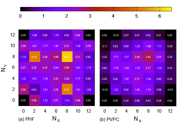
Figure 3: Ground state energy differences in MeV between approximate calculations and “exact diagonalization” from full configuration-interaction shell model, $\Delta E^{\mathrm{approx}}_{\mathrm{g.s}}=E^{\mathrm{approx}}_{\mathrm{g.s.}}-E^{\mathrm{SM}}_{\mathrm{g.s.}}$, for all even-even nuclei in $1s0d$ shell. Panel (a) is for angular momentum-projected Hartree Fock results, and Panel (b) is for the PVPC in this work. See text for more details.

Aside from the ground state energies, it is interesting to see how well the excitation energies are approximated by such “projection after variation” methods, as was done recently for PHF Lauber et al. (2021). As a test we investigate yrast bands of even-even isotopes of silicon, using results from PVPC, PHF and full configuration-interaction shell model. Fig. 4 demonstrates both PHF and PVPC generate good yrast-band excitation spectra for open-shell nuclei. For semi-magic nuclei ^22,34Si, Hartree-Fock minima are spherical and thus PHF trivially generates only the ground state $0^{+}_{1}$. The PVPC generates yrast bands of ^22,34Si close to that of the shell model. For ³⁴Si both the PVPC and the shell model predict the $2^{+}_{1}$ excitation energy higher than the experimental value Nica and Singh (2012). We note that approximate excitation energies do not follow a variational principle and can be lower than that of the full configuration shell model. Although it is not shown here, the yrare and higher bands of PVPC can be worse, and likely need more reference states to improve, such as from coexisting local minima Lauber et al. (2021).

As a test of the approximate wavefunctions, we present in Table 1 the $B(E2,I+2\rightarrow I)$ values for silicon isotopes corresponding to Fig. 4. While projected states can reproduce the transition strengths qualitatively, there can still be discrepancies, for example $B(E2,4^{+}_{1}\rightarrow 2^{+}_{1})$ of ²⁶Si from the PVPC is about $1/6$ of that from the shell model; again, this may be improved by additional reference condensates.

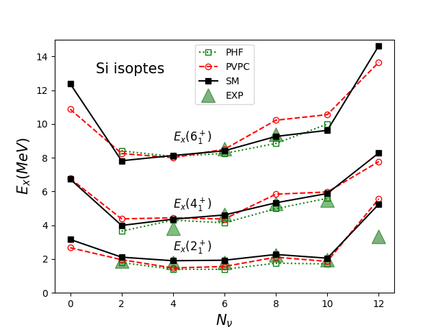
Figure 4: Excitation energy of yrast states of even-even nuclei ^22-34Si. ”PHF” stands for angular momentum projected Hartree-Fock, ”PVPC” stands for angular momentum projection after variation of a pair condensate (this work), ”SM” stands for the full configuration-interaction shell model. All these three methods use the same occupation space $1s0d$, and the same interaction: USDBBrown and Richter (2006). Experimental data are from Kanno et al. (2002); Basunia and Hurst (2016); Shamsuzzoha Basunia (2013, 2010); Dufour et al. (1986); Nica and Singh (2012).

Nuclide	Method	$2^{+}_{1}\rightarrow 0^{+}_{1}$	$4^{+}_{1}\rightarrow 2^{+}_{1}$	$6^{+}_{1}\rightarrow 4^{+}_{1}$
22Si	SM	33.32	16.96	13.07
	PVPC	32.28	14.10	14.81
24Si	SM	44.19	23.89	17.58
	PVPC	37.13	25.60	41.66
26Si	SM	44.64	11.29	41.94
	PVPC	37.34	60.31	70.56
28Si	SM	78.48	110.4	94.71
	PVPC	83.47	116.3	119.2
30Si	SM	46.52	15.94	32.70
	PVPC	48.33	33.68	78.15
32Si	SM	43.52	67.11	52.70
	PVPC	37.54	64.06	66.85
34Si	SM	34.91	16.80	6.14
	PVPC	30.78	14.93	1.50

Table 1: $B(E2)$ values for silicon isotopes in units of $e^{2}\,\mathrm{fm}^{4}$. SM stands for full configuration shell model with “exact” diagonalization, while PVPC stands for projection and variation of one pair condensate. Both methods use the USDB interaction in the $1s0d$ shell. Effective charges are set as $e_{p}=1.5e,e_{n}=0.5e$.

III.2 The $1p0f$ shell

We use the GX1A interaction in the $1p0f$ shell Honma et al. (2002, 2005). We find the PVPC ground state energy is typically $1$-$2$ MeV above the exact shell model value. Here we give results of Ca, Ti, Cr isotones with $N=26,28$, to show that PVPC generates spectrum of pairing-like and vibrational-like spectrum self-consistently, as the number of valence particles increase. Then we demonstrate backbending in the rotational yrast spectrum of ⁵²Fe, with the pair condensate as the intrinsic wave function.

III.2.1 ^46,48Ca, ^48,50Ti, ^50,52Cr

Fig. 5 presents the low-lying spectra of $N=26,28$ isotones ^46,48Ca, ^48,50Ti, ^50,52Cr, using results from PVPC, PHF, and the full configuration shell model, as well as comparison with experiment which illustrates the quality of the shell model interaction. For the spherical nucleus ⁴⁸Ca, the fraction $f_{J}$ for $J=0$ is more than $99.9\%$, as shown in Fig. 2; nonetheless, the $J>0$ states projected out with $f_{J}<0.1\%$ turn out to be unexpectedly accurate. We see seniority-like spectra with a substantial pairing gap between $0^{+}_{1}$ and $2^{+}_{1}$, and the $3+,4+,5+$ levels clustered close to $2^{+}_{1}$. Although it is not shown on Fig. 5, the $0^{+}_{1}$ of ^46,48Ca is $\approx 0.3$ MeV above the “exact” shell model ground state, while other nuclei in the picture have ground state energies $1\sim 2$ MeV above shell model results. The excitation spectra of the “ground band” from all three theoretical methods agree qualitatively, except that PHF does not generate $J>0$ states for ⁴⁸Ca, with a spherical Hartree-Fock energy about $0.4$ MeV above the exact shell model value.

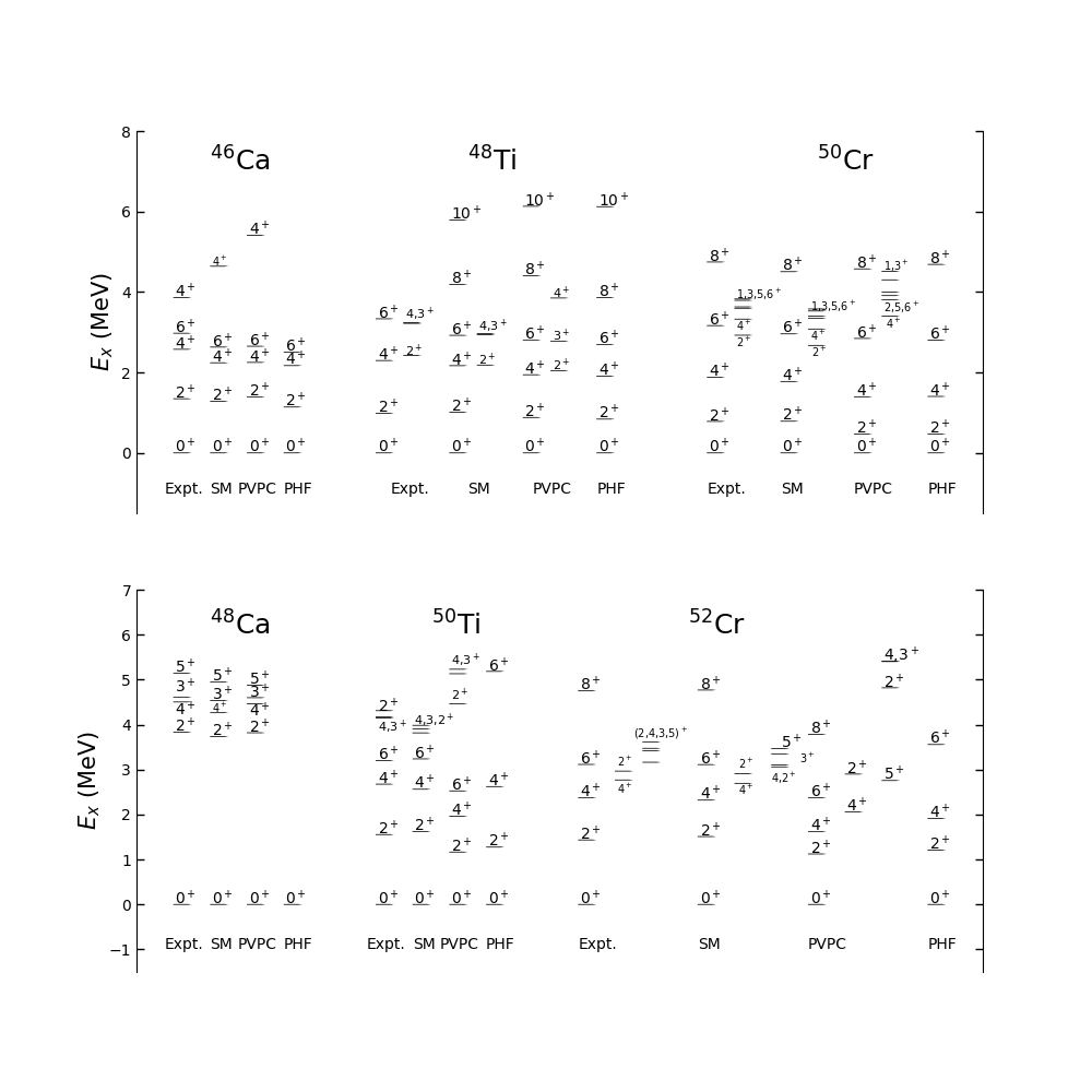
Figure 5: Low-lying spectrum of $N=26,28$ isotones: ^46,48Ca, ^48,50Ti, ^50,52Cr. All theoretical results are produced with the interaction GX1A Honma et al. (2002, 2005) in the $1p0f$ shell. Experimental results are from Wu (2000); Burrows (2006); Chen and Singh (2019); Dong and Junde (2015).

Table 2 provides the corresponding $B(E2)$ values for the nuclides in Fig. 5. The agreement between PVPC and the full configuration shell model supports the quality of PVPC wavefunctions, although we note that $B(E2;6^{+}_{1}\rightarrow 4^{+}_{1})$ of ⁴⁸Ca by PVPC is far from the shell model result. We note that the shell model spectra of ⁴⁸Ca has four $6^{+}$ states with an excitation energy between 7.7 and 9 MeV, while PVPC yields only one $6^{+}$ state in the same energy range. Therefore the $6^{+}_{1}$ by PVPC is likely a mixture of those shell model $6^{+}$ states, a possible origin for the underestimation of $B(E2;6^{+}_{1}\rightarrow 4^{+}_{1})$.

Nucleus	Method	$2^{+}_{1}\rightarrow 0^{+}_{1}$	$4^{+}_{1}\rightarrow 2^{+}_{1}$	$6^{+}_{1}\rightarrow 4^{+}_{1}$	Nucleus	Method	$2^{+}_{1}\rightarrow 0^{+}_{1}$	$4^{+}_{1}\rightarrow 2^{+}_{1}$	$6^{+}_{1}\rightarrow 4^{+}_{1}$
46Ca	SM	7.72	6.02	3.08	48Ca	SM	10.12	1.99	4.03
	PVPC	7.31	4.10	2.16		PVPC	9.10	1.76	0.36
48Ti	SM	87.89	126.06	51.28	50Ti	SM	85.20	83.10	39.84
	PVPC	84.67	116.36	113.57		PVPC	65.80	58.77	19.87
50Cr	SM	184.85	261.43	221.87	52Cr	SM	142.31	91.94	45.91
	PVPC	190.33	257.78	266.68		PVPC	102.8	89.00	56.39

Table 2: $B(E2)$ value of ⁴⁸Ca, ⁵⁰Ti, ⁵²Cr, ⁵²Fe in $e^{2}fm^{4}$. The PVPC and the shell model both use the GX1A interactions Honma et al. (2002, 2005), with effective charges $e_{p}=1.5e,e_{n}=0.5e$, and oscillator length $A^{1/6}$ fm.

III.2.2 Backbending in ⁵²Fe

While many methods using angular momentum projection produce good rotational bands, e.g. projected Hartree-Fock Johnson and O’Mara (2017) and the projected shell model Sun (2016), a more stringent test is backbending. For a simple rotor picture, the excitation energy of a yrast state $E_{x}(J^{+}_{1})$ is proportional to $J(J+1)$, but both experiment and theory see abrupt changes in the moment of inertia and thus the yrast spectrum deviates from the simple $J(J+1)$ rule. One explanation of this is pair breaking due to the increasing Coriolis force Ring and Shuck (1980). In Fig. 6 we show yrast energies of ⁵²Fe, from PVPC with a pair condensate playing the role of the intrinsic state, and that from exact diagonalization with the shell model. The PVPC energies are about $1$ MeV or more above the full configuration shell model energies, but both PVPC and the shell model exhibits two backbends. The PVPC curve shows more abrupt changes than the shell model. The change for $J>12$ is likely because 6 valence protons and 6 valence neutrons restricted to the $0f_{7/2}$ orbit have a maximum angular momentum of 12.

Although we do not show it, cranked PHF also generates two kinks; without cranking, the Slater determinant of the Hartree-Fock minimum does not have components of $J\geq 12$.

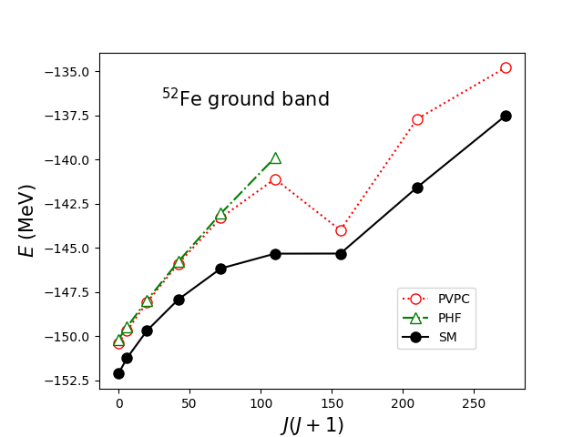
Figure 6: Backbending of yrast band of ⁵²Fe. “PVPC” is projected states from one pair condensate, “SM” is the full configuration shell model, and “PHF” the projected Hartree-Fock method. The GX1A interaction is used for the $1p0f$ shell.

III.3 The $2s1d0g_{7/2}0h_{11/2}$ shell

Fig. 7 shows the ground state band of three $N=54$ isotones. For ¹⁰⁴Sn, ¹⁰⁶Te we take the experimental data from Blachot (2007); De Frenne and Negret (2008), while the low-lying spectrum of ¹⁰⁸Xe has not been not measured. PVPC generates ground band rather close to that of the shell model. The discrepancy $\Delta E^{PVPC}_{g.s.}\equiv E^{PVPC}_{g.s.}-E^{SM}_{g.s.}$ is about $0.2,0.8,0.9$ MeV, respectively for ¹⁰⁴Sn, ¹⁰⁶Te, ¹⁰⁸Xe. As in the $1s0d$ or $1p0f$ shell, PVPC does better for semi-magic nuclei than PHF, as one might anticipate, but PHF approaches PVPC for the rotational nucleus ¹⁰⁸Xe, although the PVPC ground state energy is about $0.5$ MeV lower than that of PHF. In Table 3, the $B(E2,I^{+}_{1}\rightarrow(I-2)^{+}_{1})$ values are presented, in correspondence to Fig. 7. The $B(E2)$ values of PVPC agree with those of the shell model qualitatively. We also show the ground band of ^124,126Xe, ^126,128Ba in Fig. 8 generated with PVPC and PHF, although $0^{+}_{1}$ of both these methods appear not low enough. For all these four nuclei ^124,126Xe, ^126,128Ba the PVPC generates ground state energies less than $0.5$ MeV lower than PHF does, and the excitation energies of PVPC and PHF are mostly alike.

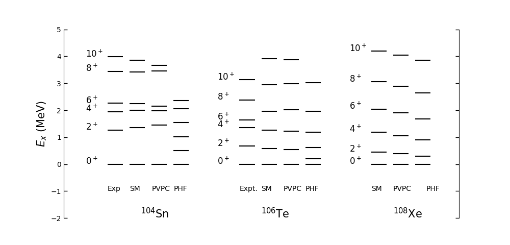
Figure 7: Ground band excitation energies of $N=54$ isotones ¹⁰⁴Sn, ¹⁰⁶Te, ¹⁰⁸Xe. Both the shell model and the PVPC use a monopole-adjusted G-matrix interaction Qi and Xu (2012), and the experimental data is from Blachot (2007); De Frenne and Negret (2008).

Nucleus	Method	$2^{+}_{1}\rightarrow 0^{+}_{1}$	$4^{+}_{1}\rightarrow 2^{+}_{1}$	$6^{+}_{1}\rightarrow 4^{+}_{1}$	$8^{+}_{1}\rightarrow 6^{+}_{1}$	$10^{+}_{1}\rightarrow 8^{+}_{1}$
104Sn	SM	42.9	40.0	14.2	18.1	30.8
	PVPC	36.1	24.5	5.4	10.8	19.6
106Te	SM	444.8	588.0	573.0	478.6	504.8
	PVPC	430.3	597.8	619.7	565.8	485.0
108Xe	SM	943.3	1277	1373	1449	1369
	PVPC	755.6	1044	963.2	901.1	1044

Table 3: $B(E2)$ value of $N=54$ isotones ¹⁰⁴Sn, ¹⁰⁶Te, ¹⁰⁸Xe in $e^{2}$ fm⁴. Both methods use a monopole-modified G-matrix interaction Qi and Xu (2012) in the $2s1d0g_{7/2}0h_{11/2}$ shell. Effective charges are set as $e_{p}=1.5e,e_{n}=0.5e$.

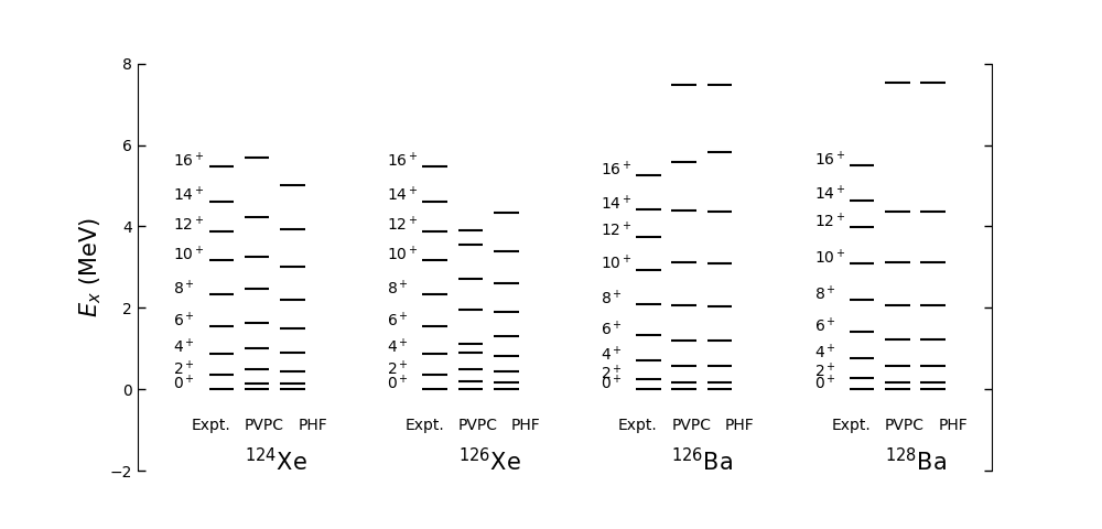
Figure 8: Ground band excitation energy of ^124,126Xe, ^126,128Ba,

IV summary

In summary, we derived formulas for projection after variation of pair condensates(PVPC), implemented those formulas into codes, and present one-reference (i.e. one pair condensate for one nucleus) benchmark results. The variation of a pair condensate is time-consuming, as it takes several hours to optimize a pair condensate for ¹³²Dy in the $2s1d0g_{7/2}0h_{11/2}$ space on a 44-core machine. After finding the variational minimum, triaxial projection with the LAP technique is very quick. Because the pair condensate as a variation ansatz is more general than the Hartree-Fock, or the Hartree-Fock-Bogolyubov method, the PVPC generates semi-magic or open-shell nuclei more consistently. We benchmark results of nuclei in $1s0d,1p0f,2s1d0g_{7/2}0h_{11/2}$ shells, by comparing results of PVPC with PHF and shell model when possible. For semi-magic nuclei the PVPC generates seniority-type spectrum, satisfactorily close to shell model results. For rotational nuclei the PVPC generates rotational ground band, similar to results from the Projected Hartree-Fock method, though less than $1$ MeV lower, and with a few more states.

In future work, a benchmark comparison with the Hartree-Fock-Bogoliubov method can be interesting, as the HFB and PVPC both have intrinsic pairing structure. PVPC allows for tri-axial deformation, but due to constraint of one reference (one pair condensate), tri-axial phenemonon, such as a low $0^{+}_{2}$ in ⁷⁶Ge, is not reproduced yet. In addition, inclusion of more than one pair condensate à la generator coordinate methods can be implemented. It is also straight forward to extend the formalism to proton-neutron pair condensates, or odd valence protons/neutrons, or separate projection of proton/neutron parts as related to the scissors mode.

Appendix A Formulas for Hamiltonian matrix elements and their derivatives

To carry out the variation and projection of a pair condensate state $|\Phi\rangle\equiv(\hat{A}^{\dagger})^{n}|0\rangle$ we need a variety of matrix elements. In particular we need the normalization $\langle\Phi|\Phi\rangle$, then expectation of the Hamiltonian of that state $\langle\Phi|\hat{H}|\Phi\rangle$, and the partial derivatives of these two quantities: $\partial\langle\Phi|\Phi\rangle/\partial A_{\alpha\beta}$ and $\partial\langle\Phi|\hat{H}|\Phi\rangle/\partial A_{\alpha\beta}$. To do projection, we also need to rotate the condensate $\hat{R}(\Omega)(\hat{A}^{\dagger})^{n}|0\rangle=(\hat{A^{\prime}}^{\dagger})^{n}|0\rangle$, with coefficient matrix $A^{\prime}={\mathcal{D}}(\Omega)A{\mathcal{D}}(\Omega)^{\top}$, and to calculate the norm and Hamiltonian kernels: $\langle\hat{A}^{n}|\hat{R}(\Omega)|(\hat{A}^{\dagger})^{n}\rangle=\langle\hat{A}^{n}|(\hat{A^{\prime}}^{\dagger})^{n}\rangle$ and $\langle\hat{A}^{n}|\hat{H}\hat{R}(\Omega)|(\hat{A}^{\dagger})^{n}\rangle=\langle\hat{A}^{n}|\hat{H}|(\hat{A^{\prime}}^{\dagger})^{n}\rangle$. In this appendix we give the expressions for Hamiltonian matrix elements and their derivatives in terms of condensate overlaps including what we term impurity pairs. In Appendix B, we derive all necessary overlap formulas of condensates, with or without “impurity” pairs, completing the necessary formalism.

A.1 Hamiltonian matrix elements

The Hamiltonian matrix element, $\langle(\hat{A}_{1})^{n}|\hat{H}|(\hat{A}^{\dagger}_{2})^{n}\rangle$, consists of of one-body parts $\langle(\hat{A}_{1})^{n}|\hat{Q}|(\hat{A}^{\dagger}_{2})^{n}\rangle$, such as single particle energies, and two-body parts $\langle(\hat{A}_{1})^{n}|\hat{A}^{\dagger}_{3}\hat{A}_{4}|(\hat{A}^{\dagger}_{2})^{n}\rangle$. The one-body operator $\hat{Q}\equiv\sum_{\alpha\beta}Q_{\alpha\beta}\hat{c}^{\dagger}_{\alpha}\hat{c}_{\beta}$ has structure coefficients $Q_{\alpha\beta}$. Through commutation relations, the matrix element of a one-body operator can be expressed as an overlap,

$$\langle(\hat{A}_{1})^{n}|\hat{Q}|(\hat{A}_{2}^{\dagger})^{n}\rangle=n\langle(\hat{A}_{1})^{n-1}[\hat{A}_{1},\hat{Q}]|(\hat{A}_{2}^{\dagger})^{n}\rangle=n\langle(\hat{A}_{1})^{n-1}\hat{A}_{3}|(\hat{A}_{2}^{\dagger})^{n}\rangle,$$ (32)

where $\hat{A}_{3}\equiv{[}\hat{A}_{1},\hat{Q}{]}$, with pair structure coefficients $A_{3}=A_{1}Q+Q^{\top}A_{1}$. We term $\hat{A}_{3}$ an “impurity pair”, as it replaces one $\hat{A}_{1}$ in the bra vector $\langle(\hat{A}_{1})^{n}|$ to arrive at Eq. (32).

Similarly, the matrix element of a general two-body interaction $\hat{A}^{\dagger}_{3}\hat{A}_{4}$ can be written as

$$\langle(\hat{A}_{1})^{n}|\hat{A}^{\dagger}_{3}\hat{A}_{4}|(\hat{A}_{2}^{\dagger})^{n}\rangle = \langle\hat{A}^{n}_{1}\hat{A}_{4}|\hat{A}^{\dagger}_{3}(\hat{A}^{\dagger}_{2})^{n}\rangle+\langle\hat{A}^{n}_{1}[\hat{A}^{\dagger}_{3},\hat{A}_{4}](\hat{A}^{\dagger}_{2})^{n}\rangle$$

$$= \langle\hat{A}^{n}_{1}\hat{A}_{4}|\hat{A}^{\dagger}_{3}(\hat{A}^{\dagger}_{2})^{n}\rangle+\frac{1}{2}\mathrm{tr}\,(A_{3}A_{4})\langle\hat{A}^{n}_{1}|(\hat{A}^{\dagger}_{2})^{n}\rangle-n\langle\hat{A}^{n-1}_{1}\hat{A}_{5}|(\hat{A}^{\dagger}_{2})^{n}\rangle,$$

where $\mathrm{tr}\,(A_{3}A_{4})$ is the trace of the matrix product $A_{3}A_{4}$, and $A_{5}=A_{1}A_{3}A_{4}+A_{4}A_{3}A_{1}$. The first term on the right of Eq. (A.1), $\langle\hat{A}^{n}_{1}\hat{A}_{4}|\hat{A}^{\dagger}_{3}(\hat{A}^{\dagger}_{2})^{n}\rangle$, with two impurity pairs, is the most complicated overlap to evaluate in Eq. (A.1).

A.2 Derivatives of Hamiltonian matrix elements

To calculate derivatives $\partial\langle\hat{A}^{n}_{1}|\hat{H}|(\hat{A}^{\dagger}_{2})^{n}\rangle/\partial(A_{1})_{\alpha\beta}$ and $\partial\langle\hat{A}^{n}_{1}|(\hat{A}^{\dagger}_{2})^{n}\rangle/\partial(A_{1})_{\alpha\beta}$, we borrow from Ref. Otsuka et al. (2001) a general formalism for derivatives. Let $\hat{O}$ be an operator, e.g. 1 for overlap or $\hat{H}$ for Hamiltonian matrix elements. The matrix element of $\hat{O}$ on two pair condensates is

$$\langle\hat{A}^{n}_{1}|\hat{O}|(\hat{A}^{\dagger}_{2})^{n}\rangle.$$ (34)

Taking $\hat{A}_{1}(\lambda)=\hat{A}_{1}+\lambda\hat{\Gamma}$, where $\lambda$ is small (and, we assume, real), yields to first order

$$\langle(\hat{A}_{1}+\lambda\hat{\Gamma})^{n}|\hat{O}|(\hat{A}^{\dagger}_{2})^{n}\rangle=\langle\hat{A}^{n}_{1}|\hat{O}|(\hat{A}^{\dagger}_{2})^{n}\rangle+n\lambda\langle\hat{A}^{n-1}_{1}\hat{\Gamma}|\hat{O}|(\hat{A}^{\dagger}_{2})^{n}\rangle,$$ (35)

hence

$$\left.\frac{\partial}{\partial\lambda}\langle\hat{A}^{n}_{1}(\lambda)|\hat{O}|(\hat{A}^{\dagger}_{2})^{n}\rangle\right|_{\lambda=0}=n\langle\hat{A}^{n-1}_{1}\hat{\Gamma}|\hat{O}|(\hat{A}^{\dagger}_{2})^{n}\rangle.$$ (36)

Now $\hat{\Gamma}$ plays the role of an impurity pair. The derivative of an overlap between pair condensates is simply

$$\frac{\partial}{\partial\lambda}\langle(\hat{A}_{1}(\lambda))^{n}|(\hat{A}_{2}^{\dagger})^{n}\rangle=n\langle(\hat{A}_{1})^{n-1}\Gamma|(\hat{A}_{2}^{\dagger})^{n}\rangle,$$ (37)

while the derivative of a one-body matrix element (Eq. 32) is

$$\frac{\partial}{\partial\lambda}\langle(\hat{A}_{1})^{n}|\hat{Q}|(\hat{A}_{2}^{\dagger})^{n}\rangle=n\langle(\hat{A}_{1})^{n-1}\Gamma|[\hat{Q},\hat{A}_{2}^{\dagger}](\hat{A}_{2}^{\dagger})^{n-1}\rangle=n\langle(\hat{A}_{1})^{n-1}\Gamma|\hat{A}^{\dagger}_{3}(\hat{A}_{2}^{\dagger})^{n-1}\rangle,$$ (38)

where $\hat{A}^{\dagger}_{3}\equiv[\hat{Q},\hat{A}_{2}^{\dagger}]$, with pair structure coefficients $A_{3}=A_{2}Q^{\top}+QA_{2}$. Finally, the derivative of two-body matrix element (Eq. A.1) is

$$\frac{\partial}{\partial\lambda}\langle(\hat{A}_{1})^{n}|\hat{A}^{\dagger}_{3}\hat{A}_{4}|(\hat{A}_{2}^{\dagger})^{n}\rangle = n\langle\hat{A}^{n-1}_{1}\hat{\Gamma}|\hat{A}^{\dagger}_{3}\hat{A}_{4}|(\hat{A}^{\dagger}_{2})^{n}\rangle$$ (39)

$$= n\langle\hat{A}^{n-1}_{1}\hat{\Gamma}\hat{A}_{4}|\hat{A}^{\dagger}_{3}(\hat{A}^{\dagger}_{2})^{n}\rangle+n\,\mathrm{tr}\,(A_{3}A_{4})\langle\hat{A}_{1}^{n-1}\hat{\Gamma}|(\hat{A}^{\dagger}_{2})^{n}\rangle$$

$$-n(n-1)\langle\hat{A}^{n-2}_{1}\Gamma\hat{A}_{5}|(\hat{A}^{\dagger}_{2})^{n}\rangle,$$

where $A_{5}=A_{1}A_{3}A_{4}+A_{4}A_{3}A_{1}$. On the right side, the most complicated overlap in this work is the first term, with 3 impurity pairs. Thus the derivatives of Hamiltonian matrix elements can be computed from overlaps of pair condensates with impurity pairs, discussed in Appendix B.

Appendix B Overlap formulas

In this appendix, we give formulas for overlaps between pair condensates each with up to three impurity pairs; these are needed for Appendix A and Sec. II. We begin with a general formula that expresses the overlap for $n$-pair states in terms of matrix traces Silvestre-Brac and Piepenbring (1982); Ginocchio and Johnson (1995),

$$\langle\hat{A}_{1}\cdots\hat{A}_{n}|\hat{B}^{\dagger}_{1}\cdots\hat{B}^{\dagger}_{n}\rangle=\sum\limits^{n}_{k=1}(-2)^{-k}\sum\limits^{m_{1}+\cdots+m_{k}=n}_{m_{1}\geq m_{2}\geq\cdots\geq m_{k}}\prod_{w=1}^{k}m_{w}^{-1}\prod_{w\in\{m_{1},\cdots m_{k}\}}(R_{w}!)^{-1}$$

$$\times\sum\limits_{\left\{j_{1},\cdots,j_{n}\right\},\left\{i_{1},\cdots,i_{n}\right\}}\mathrm{tr}\,(A_{i_{1}}B_{j_{1}}\cdots A_{i_{m_{1}}}B_{j_{m_{1}}})\cdots\mathrm{tr}\,(A_{i_{n+1-m_{k}}}B_{j_{n+1-m_{k}}}\cdots A_{i_{n}}B_{j_{n}}).$$ (40)

Here $\{i_{1},\cdots,i_{n}\}$ and $\{j_{1},\cdots,j_{n}\}$ are rearrangements of $\left\{1,2,\cdots,n\right\}$, $m_{1}\geq m_{2}\geq\cdots\geq m_{k}$ is a partition of $n$, and $R_{i}$ is the degeneracy of $m_{i}$ in a partition, i.e., the number of times $m_{i}$ is repeated.

While one can carry out Eq. (40) either by commutation relations Lei et al. (2021); Silvestre-Brac and Piepenbring (1982) or by a generating function Ginocchio and Johnson (1995), here we consider the important special case of a collective pair condensate, i.e., all $n$ pairs in a state are identical:

$$\langle(\hat{A}_{1})^{n}|(\hat{A}_{2}^{\dagger})^{n}\rangle = (n!)^{2}\sum\limits_{k=1}^{n}(-2)^{-k}\sum\limits^{m_{1}+\cdots+m_{k}=n}_{m_{1}\geq m_{2}\geq\cdots\geq m_{k}}\prod_{w=1}^{k}m_{w}^{-1}\prod_{w\in\{m_{1},\cdots m_{k}\}}(R_{w}!)^{-1}\cdots$$ (41)

$$\times\mathrm{tr}\,((A_{1}A_{2})^{m_{1}})\cdots\mathrm{tr}\,((A_{1}A_{2})^{m_{k}}).$$

Therefore, to calculate one overlap between condensates as in Eq. (41), we calculate $\mathrm{tr}\,(A_{1}A_{2})$, $\cdots$, $\cdots\mathrm{tr}\,((A_{1}A_{2})^{n})$, and sum over all ordered partitions $\{m_{1},\cdots,m_{k}\}$ . The computation time is polynomial in $n$. Note when $n$ is large, e.g. $n=16$ in $2s1d0g_{7/2}0h_{11/2}$ shell (N,Z $\in[50,82]$), the summation of (41) can have cancellations of large numbers, requiring careful consideration of round-off error.

Similarly, from Eq. (40), we can obtain overlap formulas with impurity pairs. Our work here requires overlap formulas with at most three different impurity pairs:

$$\langle(\hat{A}_{1})^{n-1}A_{3}|(\hat{A}_{2}^{\dagger})^{n}\rangle$$ (42)

$$= (n-1)!n!\sum\limits_{k=1}^{N}(-2)^{-k}\sum\limits^{m_{1}+\cdots+m_{k}=n}_{m_{1}\geq m_{2}\geq\cdots\geq m_{k}}\prod_{w=1}^{k}m_{w}^{-1}\prod_{w\in\{m_{1},\cdots m_{k}\}}(R_{w}!)^{-1}\sum\limits^{k}_{r=1}m_{r}$$

$$\times\mathrm{tr}\,((A_{1}A_{2})^{m_{1}})\cdots\mathrm{tr}\,((A_{1}A_{2})^{m_{r}-1}A_{3}A_{2})\cdots\mathrm{tr}\,((A_{1}A_{2})^{m_{k}}).$$

$$\langle(\hat{A}_{1})^{n-1}A_{3}|A^{\dagger}_{4}(\hat{A}_{2}^{\dagger})^{n-1}\rangle$$ (43)

$$= ((n-1)!)^{2}\sum\limits_{k=1}^{n}(-2)^{-k}\sum\limits^{m_{1}+\cdots+m_{k}=n}_{m_{1}\geq m_{2}\geq\cdots\geq m_{k}}\prod_{w=1}^{k}m_{w}^{-1}\prod_{w\in\{m_{1},\cdots m_{k}\}}(R_{w}!)^{-1}$$

$$\times~{}~{}\left\{\sum\limits^{k}_{r=1}m_{r}\sum\limits^{m_{r}-1}_{s=0}\cdots\mathrm{tr}\,(A_{3}(A_{2}A_{1})^{s}A_{4}(A_{1}A_{2})^{m_{r}-1-s})\cdots\right.$$

$$\left.+\sum\limits^{r\neq s}_{1\leq r,s\leq k}m_{r}m_{s}\cdots\mathrm{tr}\,((A_{1}A_{2})^{m_{r}-1}A_{3}A_{2})\cdots\mathrm{tr}\,(A_{1}A_{4}(A_{1}A_{2})^{m_{s}-1})\cdots\right\}.$$

$$\langle(\hat{A}_{1})^{n-2}A_{3}A_{4}|(\hat{A}_{2}^{\dagger})^{n}\rangle$$ (44)

$$= n!(n-2)!\sum\limits_{k=1}^{n}(-2)^{-k}\sum\limits^{m_{1}+\cdots+m_{k}=n}_{m_{1}\geq m_{2}\geq\cdots\geq m_{k}}\prod_{w=1}^{k}m_{w}^{-1}\prod_{w\in\{m_{1},\cdots m_{k}\}}(R_{w}!)^{-1}$$

$$\times~{}~{}\left\{\sum\limits^{k}_{r=1}m_{r}\sum\limits^{m_{r}-2}_{s=0}\cdots\mathrm{tr}\,(A_{3}A_{2}(A_{1}A_{2})^{s}A_{4}A_{2}(A_{1}A_{2})^{m_{r}-2-s})\cdots\right.$$

$$\left.+\sum\limits^{r\neq s}_{1\leq r,s\leq k}m_{r}m_{s}\cdots\mathrm{tr}\,((A_{1}A_{2})^{m_{r}-1}A_{3}A_{2})\cdots\mathrm{tr}\,(A_{4}A_{2}(A_{1}A_{2})^{m_{r}-1})\cdots\right\}.$$

$$\langle(\hat{A}_{1})^{n-2}\hat{A}_{3}\hat{A}_{4}|\hat{A}^{\dagger}_{5}(\hat{A}_{2}^{\dagger})^{n-1}\rangle$$ (45)

$$= (n-1)!(n-2)!\sum\limits_{k=1}^{n}(-2)^{-k}\sum\limits^{m_{1}+\cdots+m_{k}=n}_{m_{1}\geq m_{2}\geq\cdots\geq m_{k}}\prod_{w=1}^{k}m_{w}^{-1}\prod_{w\in\{m_{1},\cdots m_{k}\}}(R_{w}!)^{-1}$$

$$\left\{\sum\limits^{{r\neq s\neq t}}_{1\leq r,s,t\leq k}m_{r}m_{s}m_{t}\cdots\mathrm{tr}\,(A_{3}A_{2}(A_{1}A_{2})^{m_{r}-1})\cdots\mathrm{tr}\,(A_{4}A_{2}(A_{1}A_{2})^{m_{s}-1})\cdots\mathrm{tr}\,(A_{1}A_{5}(A_{1}A_{2})^{m_{t}-1})\cdots\right.$$

$$+\sum\limits^{r\neq s}_{1\leq r,s\leq k}m_{r}m_{s}\sum\limits^{m_{r}-1}_{t=0}\cdots\mathrm{tr}\,(A_{3}(A_{2}A_{1})^{t}A_{5}(A_{1}A_{2})^{m_{r}-1-t})\cdots\mathrm{tr}\,(A_{4}A_{2}(A_{1}A_{2})^{m_{s}-1})\cdots$$

$$+\sum\limits^{r\neq s}_{1\leq r,s\leq k}m_{r}m_{s}\sum\limits^{m_{r}-1}_{t=0}\cdots\mathrm{tr}\,(A_{4}(A_{2}A_{1})^{t}A_{5}(A_{1}A_{2})^{m_{r}-1-t})\cdots\mathrm{tr}\,(A_{3}A_{2}(A_{1}A_{2})^{m_{s}-1})\cdots$$

$$+\sum\limits^{r\neq s}_{1\leq r,s\leq k}m_{r}m_{s}\sum\limits^{m_{r}-2}_{t=0}\cdots\mathrm{tr}\,(A_{3}A_{2}(A_{1}A_{2})^{t}A_{4}A_{2}(A_{1}A_{2})^{m_{r}-2-t})\cdots\mathrm{tr}\,(A_{1}A_{5}(A_{1}A_{2})^{m_{s}-1})\cdots$$

$$\left.+\sum\limits^{k}_{r=1}m_{r}\sum\limits^{m_{r}-1}_{s=1}\sum\limits^{m_{r}}_{t=1}\cdots\mathrm{tr}\,(A_{3}A_{2}A_{1}A_{2}\cdots[A_{5}]_{2t}\cdots[A_{4}]_{2s+1}\cdots A_{1}A_{2})\cdots\right\},$$

where $[A_{5}]_{2t}$ means $A_{5}$ is at position $2t$, $[A_{4}]_{2s+1}$ means $A_{4}$ is at position $2s+1$ in the matrix product.

References

- Bohr and Mottelson (1998) A. N. Bohr and B. R. Mottelson, Nuclear Structure (In 2 Volumes) (World Scientific Publishing Company, Singapore, 1998).
- Ring and Shuck (1980) P. Ring and P. Shuck, The Nuclear Many-Body Problem (Springe, 1980).
- Frauendorf and Dönau (2014) S. Frauendorf and F. Dönau, Phys. Rev. C 89, 014322 (2014).
- Ayangeakaa et al. (2013) A. D. Ayangeakaa, U. Garg, M. D. Anthony, S. Frauendorf, J. T. Matta, B. K. Nayak, D. Patel, Q. B. Chen, S. Q. Zhang, P. W. Zhao, B. Qi, J. Meng, R. V. F. Janssens, M. P. Carpenter, C. J. Chiara, F. G. Kondev, T. Lauritsen, D. Seweryniak, S. Zhu, S. S. Ghugre, and R. Palit, Phys. Rev. Lett. 110, 172504 (2013).
- Xu et al. (2017) C. Xu, G. Röpke, P. Schuck, Z. Ren, Y. Funaki, H. Horiuchi, A. Tohsaki, T. Yamada, and B. Zhou, Phys. Rev. C 95, 061306(R) (2017).
- Surman et al. (2016) Surman, R., Mumpower, M., R., Aprahamian, A., McLaughlin, G., and C., Progress in Particle & Nuclear Physics (2016).
- Kajino et al. (2019) T. Kajino, W. Aoki, A. Balantekin, R. Diehl, M. Famiano, and G. Mathews, Progress in Particle and Nuclear Physics 107, 109 (2019).
- Meng (2016) J. Meng, International Review of Nuclear Physics-Vol. 10: Relativistic Density Functional for Nuclear Structure (World Scientific, 2016).
- Bally and Bender (2021) B. Bally and M. Bender, Phys. Rev. C 103, 024315 (2021).
- Sánchez-Fernández et al. (2021) A. Sánchez-Fernández, B. Bally, and T. R. Rodríguez, Phys. Rev. C 104, 054306 (2021).
- Bally et al. (2019) B. Bally, A. Sánchez-Fernández, and T. R. Rodríguez, Phys. Rev. C 100, 044308 (2019).
- Shimizu et al. (2021) N. Shimizu, T. Mizusaki, K. Kaneko, and Y. Tsunoda, Phys. Rev. C 103, 064302 (2021).
- Iachello and Arima (2006) F. Iachello and A. Arima, The Interacting Boson Model (Cambridge Univ Pr, 2006).
- Sun et al. (2000) Y. Sun, K. Hara, J. A. Sheikh, J. G. Hirsch, V. Velázquez, and M. Guidry, Phys. Rev. C 61, 064323 (2000).
- Otsuka et al. (2001) T. Otsuka, M. Honma, T. Mizusaki, N. Shimizu, and Y. Utsuno, Prog. Part. Nucl. Phys. 47, 319 (2001).
- Caurier et al. (2005) E. Caurier, G. Martínez-Pinedo, F. Nowacki, A. Poves, and A. P. Zuker, Rev. Mod. Phys. 77, 427 (2005).
- Brown (2001) B. Brown, Progress in Particle and Nuclear Physics 47, 517 (2001).
- Brown and Richter (2006) B. A. Brown and W. A. Richter, Phys. Rev. C 74, 034315 (2006).
- Honma et al. (2002) M. Honma, T. Otsuka, B. A. Brown, and T. Mizusaki, Phys. Rev. C 65, 061301(R) (2002).
- Honma et al. (2005) M. Honma, T. Otsuka, B. A. Brown, and T. Mizusaki, The European Physical Journal A - Hadrons and Nuclei 25, 499 (2005).
- Talmi (1993) I. Talmi, Simple Models of Complex Nuclei (Contemporary Concepts in Physics) (CRC Press, 1993).
- Jia (2019) L. Y. Jia, Phys. Rev. C 99, 014302 (2019).
- Jia (2016) L. Y. Jia, Phys. Rev. C 93, 064307 (2016).
- Jia (2015) L. Y. Jia, Journal of Physics G: Nuclear and Particle Physics 42, 115105 (2015).
- Zhao and Arima (2014) Y. Zhao and A. Arima, Physics Reports 545, 1 (2014), nucleon-pair approximation to the nuclear shell model.
- Higashiyama et al. (2002) K. Higashiyama, N. Yoshinaga, and K. Tanabe, Phys. Rev. C 65, 054317 (2002).
- He et al. (2020) B. C. He, L. Li, Y. A. Luo, Y. Zhang, F. Pan, and J. P. Draayer, Phys. Rev. C 102, 024304 (2020).
- Lei et al. (2021) Y. Lei, Y. Lu, and Y. M. Zhao, Chinese Physics C 45, 054103 (2021) (2021).
- Otsuka et al. (1978) T. Otsuka, A. Arima, F. Iachello, and I. Talmi, Physics Letters B 76, 139 (1978).
- Johnson and Ginocchio (1994) C. W. Johnson and J. N. Ginocchio, Phys. Rev. C 50, R571 (1994).
- Ginocchio and Johnson (1995) J. Ginocchio and C. Johnson, Physical Review C 51, 1861 (1995), cited By 9.
- Fu and Johnson (2020) G. Fu and C. W. Johnson, Physics Letters B 809, 135705 (2020).
- Fu and Johnson (2021) G. J. Fu and C. W. Johnson, Phys. Rev. C 104, 024312 (2021).
- Lei et al. (2020) Y. Lei, H. Jiang, and S. Pittel, Phys. Rev. C 102, 024310 (2020).
- Mizusaki and Schuck (2021) T. Mizusaki and P. Schuck, Phys. Rev. C 104, L031305 (2021).
- Coleman (1965) A. J. Coleman, Journal of Mathematical Physics 6, 1425 (1965), https://doi.org/10.1063/1.1704794 .
- Rowe et al. (1991) D. J. Rowe, T. Song, and H. Chen, Phys. Rev. C 44, R598 (1991).
- Chen et al. (1995) H. Chen, T. Song, and D. Rowe, Nuclear Physics A 582, 181 (1995).
- Johnson and O’Mara (2017) C. W. Johnson and K. D. O’Mara, Phys. Rev. C 96, 064304 (2017).
- Johnson and Jiao (2019) C. W. Johnson and C. Jiao, Journal of Physics G Nuclear & Particle Physics 46 (2019).
- Qi and Xu (2012) C. Qi and Z. X. Xu, Phys. Rev. C 86, 044323 (2012).
- Galassi et al. (2019) M. Galassi, J. Davies, J. Theiler, B. Gough, G. Jungman, P. Alken, M. Booth, F. Rossi, and R. Ulerich, GNU Scientific Library (gnu, 2019).
- Fletcher (1984) R. Fletcher, SIAM Review 26, 143–144 (1984).
- Sun (2016) Y. Sun, Phys. Scr. 91 (2016) 043005 (23pp) (2016).
- Yao et al. (2010) J. M. Yao, J. Meng, P. Ring, and D. Vretenar, Physical Review C 81, 044311 (2010).
- Rodríguez-Guzmán et al. (2002) R. Rodríguez-Guzmán, J. Egido, and L. M. Robledo, Nuclear Physics A 709 (2002) 201–235 (2002).
- Edmonds (1957) A. R. Edmonds, Angular momentum in quantum mechanics, edited by Princeton (Princeton University Press, 1957).
- Sheikh et al. (2002) J. A. Sheikh, P. Ring, E. Lopes, and R. Rossignoli, Phys. Rev. C 66, 044318 (2002).
- Johnson et al. (2013) C. W. Johnson, W. Ormand, and P. G. Krastev, Computer Physics Communications 184 (2013).
- Lauber et al. (2021) S. M. Lauber, H. C. Frye, and C. W. Johnson, Journal of Physics G: Nuclear and Particle Physics 48, 095107 (2021).
- Johnson et al. (2020) C. W. Johnson, K. A. Luu, and Y. Lu, Journal of Physics G: Nuclear and Particle Physics 47, 105107 (2020).
- Nica and Singh (2012) N. Nica and B. Singh, Nuclear Data Sheets 113, 1563 (2012).
- Kanno et al. (2002) S. Kanno, T. Gomi, T. Motobayashi, K. Yoneda, N. Aoi, Y. Ando, H. Baba, K. Demichi, Z. Fulop, U. Futakami, H. Hasegawa, Y. Higurashi, K. Ieki, N. Imai, N. Iwasa, H. Iwasaki, T. Kubo, S. Kubono, M. Kunibu, Y. U. Matsuyama, S. Michimasa, T. Minemura, H. Murakami, T. Nakamura, A. Saito, H. Sakurai, M. Serata, S. Shimoura, T. Sugimoto, E. Takeshita, S. Takeuchi, K. Ue, K. Yamada, Y. Yanagisawa, A. Yoshida, and M. Ishihara, Prog.Theor.Phys.(Kyoto) , Suppl. 146, 575 (2002).
- Basunia and Hurst (2016) M. Basunia and A. Hurst, Nuclear Data Sheets 134, 1 (2016).
- Shamsuzzoha Basunia (2013) M. Shamsuzzoha Basunia, Nuclear Data Sheets 114, 1189 (2013).
- Shamsuzzoha Basunia (2010) M. Shamsuzzoha Basunia, Nuclear Data Sheets 111, 2331 (2010).
- Dufour et al. (1986) J. P. Dufour, R. Del Moral, A. Fleury, F. Hubert, D. Jean, M. S. Pravikoff, H. Delagrange, H. Geissel, and K. H. Schmidt, Z.Phys. A324, 487 (1986).
- Wu (2000) S.-C. Wu, Nuclear Data Sheets 91, 1 (2000).
- Burrows (2006) T. Burrows, Nuclear Data Sheets 107, 1747 (2006).
- Chen and Singh (2019) J. Chen and B. Singh, Nuclear Data Sheets 157, 1 (2019).
- Dong and Junde (2015) Y. Dong and H. Junde, Nuclear Data Sheets 128, 185 (2015).
- Blachot (2007) J. Blachot, Nuclear Data Sheets 108, 2035 (2007).
- De Frenne and Negret (2008) D. De Frenne and A. Negret, Nuclear Data Sheets 109, 943 (2008).
- Silvestre-Brac and Piepenbring (1982) B. Silvestre-Brac and R. Piepenbring, Phys. Rev. C 26, 2640 (1982).