University of Mannheim

Master’s Thesis

High Dimensional Optimization

through the Lens of Machine Learning

by
Felix Benning

born 27 November 1996 in Nürtingen
student ID 1501817

School of Business Informatics and Mathematics
Supervisor: Prof. Dr. Leif Döring

Date of Submission: 20.12.2021

Declaration of Authorship

I hereby declare that the thesis submitted is my own unaided work. All direct or indirect sources used are acknowledged as references.

This thesis was not previously presented to another examination board and has not been published.

City, Date Signature

Introduction

Optimization in Machine Learning

In statistics or machine learning we usually want to find some model which “best describes” our data. So let $f_{w}(X)$ be a prediction for $Y$, parametrized by weights $w$, where $Z=(X,Y)$ is drawn from a distribution $\mathcal{D}$ of real world examples. We formalize the prediction error of our parameter $w$ with a loss function $l(w,z)$, e.g. a squared loss

$$l(w,z):=(f_{w}(x)-y)^{2}.$$ (1)

Then we want to minimize the expected loss over all (possible) examples, i.e. “(theoretical) risk”

$$\mathcal{L}(w):=\mathbb{E}_{Z\sim\mathcal{D}}[l(w,Z)].$$

In general, we do not have access to this expected loss. Instead we usually assume to be in possession of only a sample $\mathcal{S}=(Z_{1},\dots,Z_{S})$ of data, drawn (independently) from distribution $\mathcal{D}$. This gives rise to the “empirical risk”

$$\mathcal{L}_{\mathcal{S}}(w):=\frac{1}{S}\sum_{k=1}^{S}l(w,Z_{k})=\mathbb{E}_{Z\sim\mathcal{D}_{\mathcal{S}}}[l(w,Z)],$$ (2)

where $\mathcal{D}_{\mathcal{S}}$ is the empirical distribution generated by sampling uniformly from the set $\mathcal{S}$. The empirical risk usually approaches the theoretical risk as $S\to\infty$, since some law of large number is usually applicable (e.g. if we sample from $\mathcal{S}$ independently). Thus the next best thing to minimizing $\mathcal{L}$ is often to minimize $\mathcal{L}_{\mathcal{S}}$. In the case of a linear model

$$f_{w}(x)=\langle x,w\rangle$$

minimizing the empirical risk (2) induced by a square loss (1)

$$\mathcal{L}_{\mathcal{S}}(w)=\frac{1}{S}\sum_{k=1}^{S}(f_{w}(X_{k})-Y_{k})^{2}=\frac{1}{S}\|\mathbf{X}^{T}w-\mathbf{Y}\|^{2}$$

can be done analytically, resulting in the well known least squared regression

$$w_{*}=(\mathbf{X}^{T}\mathbf{X})^{-1}\mathbf{X}^{T}\mathbf{Y}\quad\text{where}\quad\begin{aligned} \mathbf{X}&=(X_{1},\dots,X_{S})^{T}\\ \mathbf{Y}&=(Y_{1},\dots,Y_{S})^{T}\end{aligned}.$$

But this is not possible in general. And even if it was possible, it might still be difficult to come up with the solution, slowing down experimentation with different types of models. We are therefore interested in (numeric) algorithms which can minimize arbitrary loss functions.

This train of thought leads us to various “black box” models where we assume no knowledge of the loss function itself but assume we have some form of oracle telling us things about the loss function. “Zero order oracles” allow us to evaluate the loss function at a particular point, i.e. retrieve $\mathcal{L}(w)$ for any $w$ at a fixed cost. “First order oracles” provide us not only with $\mathcal{L}(w)$ but also with $\nabla\mathcal{L}(w)$, and so on.

In some sense these black box models are extremely wasteful as we do not utilize any of the inherent structure of our model. “Structural optimization” addresses this problem and opens up the black box and makes further assumptions about the loss function. Proximal methods for example assume that some form of convex regularization function (e.g. distance penalty) is part of our overall loss function [[, e.g.]]bottouOptimizationMethodsLargeScale2018:

$$\mathcal{L}(w)=F(w)+\lambda\underbrace{\Omega(w)}_{\mathclap{\text{regularizer}}}.$$

Nevertheless we will mostly navigate around structural optimization in this work, only touching on it again with “mirror descent” in Remark 1.3.3.

We will also assume that the set of possible weights is a real vector space $\mathbb{R}^{d}$. Since projections $\Pi_{\Omega}$ to convex subsets $\Omega$ are contractions [10, Lemma 3.1], i.e.

$$\|\Pi_{\Omega}(x)-\Pi_{\Omega}(y)\|\leq\|x-y\|,$$

they can often be applied without any complications to the proofs for unbounded optimization we will cover, which show a reduction in the distance to the minimum

$$\|w_{n+1}-w_{*}\| =\|\Pi_{\Omega}(\tilde{w}_{n+1})-\Pi_{\Omega}(w_{*})\|\leq\|\tilde{w}_{n+1}-w_{*}\|$$

$$\leq\dots\text{ [unbounded arguments] }$$

$$\leq\|w_{n}-w_{*}\|.$$

The next section will explain why we will mostly skip zero order optimization.

Zero Order Optimization

If we assume an infinite number of possible inputs $w$, it does not matter how often and where we sample $\mathcal{L}$, there is always a different $w$ where $\mathcal{L}$ might be arbitrarily lower (see various “No-Free-Lunch Theorems”). We must therefore start making assumptions about $\mathcal{L}$, to make this problem tractable.

Grid Search

It is reasonable to assume that the value of our loss $\mathcal{L}$ at some point $w$ will not differ much from the loss of points in close proximity. Otherwise we would have to sample every point, which is not possible for continuous and thus infinite parameter sets. This assumption is continuity of the loss $\mathcal{L}$. One possible formulation is “$K$-Lipschitz continuity”

$$|\mathcal{L}(w_{1})-\mathcal{L}(w_{2})|<K|w_{1}-w_{2}|.$$

And while Lipschitz continuity is sufficient to find an $\epsilon$-solution $\hat{w}$ inside a unit (hyper-)cube

$$\mathcal{L}(\hat{w})\leq\inf_{0\leq w_{i}\leq 1}\mathcal{L}(w)+\epsilon$$

in a finite number of evaluations of the loss, it still requires a full “grid search” (i.e. tiling our parameter set with a grid into (tiny) cells and trying out one point for every cell) with time complexity [50, pp. 12,13]

$$\left(\left\lfloor\frac{K}{2\epsilon}\right\rfloor+1\right)^{d}$$

where $d$ is the dimension of $w$. The fact that grid search is sufficient can be seen by tiling the space into a grid and asking the oracle for the value of the loss function at each center. If the minimum is in some tile, the Lipschitz continuity forces the center of that tile to be $\epsilon$ close to it [[, cf.]p. 11]nesterovLecturesConvexOptimization2018.

The fact that this is necessary can be seen by imagining a “resisting oracle” which places the minimum in just the last grid element where we look [[, cf.]p. 13]nesterovLecturesConvexOptimization2018. The exponential increase of complexity in the dimension makes the problem intractable for even mild dimensions and precisions (e.g. $d=11$, $\epsilon=0.01$, $K=2$ implies millions of years of computation).

Other Algorithms

There are more sophisticated zero order optimization techniques than grid search like “simulated annealing” [[, e.g.]]bouttierConvergenceRateSimulated2019 or “evolutionary algorithms” [[, e.g.]]heConditionsConvergenceEvolutionary2001. But in the end they all scale relatively poor in the dimension. Calculating the (sub-)gradient on the other hand scales only linearly in the dimension. Calculating the second derivative (Hessian) requires $O(d^{2})$ operations, and doing something useful with it (e.g. solving a linear equation) usually causes $O(d^{3})$ operations. For this reason first order methods seem most suited for high dimensional optimization, as their convergence guarantees are independent of the dimension. But there are attempts to make second order methods viable by avoiding the calculation of the Hessian. These methods are usually called “Quasi Newton methods” of which we will sketch the most common methods in Chapter 4.

Related Work

A similar review was conducted by [5] with a stronger focus on second order methods but only passing interest in momentum methods which are quite successful in practice. The second half of [50] introduces more ideas for structural optimization, the first half covers both first order and second order methods extensively but does not consider stochasticity much and provides little intuition. A review with heavier focus on geometric methods (Section 4.2) was conducted by [10].

Readers Guide

In Chapter 1 we will review the well established method of gradient descent which can minimize deterministic functions. It might be tempting to skip this chapter, but note that this chapter introduces important building blocks we will use in subsequent chapters. We prove convergence of gradient descent mostly as motivation for these building blocks. The convergence proofs themselves are actually very short.

The complexity bounds in Section 1.8 on the other hand, are not required for subsequent chapters. Neither is the loss surface analysis in Section 1.6 and backtracking in Section 1.7, but they motivate assumptions we make.

While gradient descent is applicable to $\mathcal{L}_{\mathcal{S}}$, i.e. allows us to minimize empirical risk (2), we will question this approach in Chapter 2 where we show that it is possible to minimize $\mathcal{L}$ itself, provided we have an infinite supply of samples. If we start to reuse samples we would just end up minimizing $\mathcal{L}_{\mathcal{S}}$ again.

In Chapter 3 we will discuss methods to speed up gradient descent. This chapter is mostly independent of Chapter 2, so they can be read in any order.

Chapter 4 provides a review of all the methods we did not have time to go over in detail. This review should provide enough intuition to understand their importance, but we will skip convergence proofs entirely and sometimes only sketch the ideas.

Chapter 1 Gradient Descent (GD)

One relatively obvious way to utilize the gradient information $\nabla\mathcal{L}(w)$, provided by first order oracles, is to incrementally move in the direction of steepest descent [12], i.e.

$$w_{n+1}=w_{n}-h\nabla\mathcal{L}(w_{n}).$$ (gradient descent)

Where $h$ denotes the “learning rate”. A useful way to look at this equation is to notice that it is the discretization of an ordinary differential equation (ODE)

$$\frac{d}{dt}w_{n}\approx\frac{w_{n+1}-w_{n}}{h}=-\nabla\mathcal{L}(w_{n}),$$

if we view the learning rate $h$ as a time delta between times $t_{n}$ and $t_{n+1}$ with $t_{n}=nh$. As then for $h\to 0$ we arrive at the ODE in time $t$

$$\dot{w}(t)=\frac{d}{dt}w(t)=-(\nabla_{w}\mathcal{L})(w(t)).$$ (gradient flow)

That we are taking the gradient with respect to $w$, will from now on be implied. With the gradient flow equation and the fundamental theorem of analysis we get

$$\mathcal{L}(w(t_{1}))-\mathcal{L}(w(t_{0})) =\int_{t_{0}}^{t_{1}}\nabla\mathcal{L}(w(s))\cdot\dot{w}(s)ds=\int_{t_{0}}^{t_{1}}-\|\nabla\mathcal{L}(w(s))\|^{2}ds\leq 0,$$ (1.1)

which implies a decreasing loss sequence

$$\mathcal{L}(w(t_{0}))\geq\mathcal{L}(w(t_{1}))\geq\dots\geq\inf_{w}\mathcal{L}(w)\geq 0$$

implying convergence of $\mathcal{L}(w(t))$. But it does not necessitate a convergent $w(t)$ nor convergence to $\inf_{w}\mathcal{L}(w)$. This highlights why there are three different types of convergence we are interested in

Convergence of the Weights

to a (the) minimum $w_{*}$

$$\|w_{n}-w_{*}\|\to 0\qquad(n\to\infty),$$

Convergence of the Loss

$$|\mathcal{L}(w_{n})-\mathcal{L}(w_{*})|=\mathcal{L}(w_{n})-\mathcal{L}(w_{*})\to 0,$$

Convergence of the Gradient

$$\|\nabla\mathcal{L}(w_{n})\|=\|\nabla\mathcal{L}(w_{n})-\nabla\mathcal{L}(w_{*})\|\to 0.$$

1.1 Visualizing the 2nd Taylor Approximation

To build some intuition what leads to convergence of the weights let us consider more simple cases. For the second order Taylor approximation $T_{2}\mathcal{L}$ of the loss $\mathcal{L}$

$$\mathcal{L}(w+x)\approx T_{2}\mathcal{L}(w+x)=\mathcal{L}(w)+x^{T}\nabla\mathcal{L}(w)+\tfrac{1}{2}x^{T}\nabla^{2}\mathcal{L}(w)x,$$ (1.2)

we can use the first order condition, i.e. set the first derivative to zero

$$\nabla T_{2}\mathcal{L}(w+x)=\nabla\mathcal{L}(w)+\nabla^{2}\mathcal{L}(w)x\;\mkern-5.0mu plus -5.0mu\mathop{=}\limits^{!}\;\mkern-5.0mu plus -5.0mu0$$ (1.3)

to find the minimum

$$\hat{x}=-(\nabla^{2}\mathcal{L}(w))^{-1}\nabla\mathcal{L}(w).$$ (1.4)

This assumes our Hessian $\nabla^{2}\mathcal{L}(w)$ exists and is positive definite (all eigenvalues are positive), which also means it is invertible. Plugging (1.4) into

$$\nabla T_{2}\mathcal{L}(w+x)=\nabla^{2}\mathcal{L}(w)(x-\hat{x}).$$

and comparing it to (1.3) best explains where it comes from. Similarly we can rewrite the original Taylor approximation (1.2) using (1.4)

$$T_{2}\mathcal{L}(w+x) \mathrel{\smashoperator[l]{\mathop{=}_{}^{(\ref{eq: newton minimum approx relative coords})}}}\mathcal{L}(w)-x^{T}\nabla^{2}\mathcal{L}(w)\hat{x}+\tfrac{1}{2}x^{T}\nabla^{2}\mathcal{L}(w)x$$

$$=\underbrace{\mathcal{L}(w)-\tfrac{1}{2}\hat{x}\nabla^{2}\mathcal{L}(w)\hat{x}}_{=:c(w)\text{ (const.)}}+\tfrac{1}{2}(x-\hat{x})^{T}\nabla^{2}\mathcal{L}(w)(x-\hat{x}).$$

So far we have expressed the location of the minimum $\hat{x}$ of the Taylor approximation only relative to $w$. To obtain its absolute coordinates $\theta:=w+x$ we define

$$\hat{w}:=w+\hat{x}\;\mkern-5.0mu plus -5.0mu\mathop{=}\limits^{(\ref{eq: newton minimum approx relative coords})}\;\mkern-5.0mu plus -5.0muw-(\nabla^{2}\mathcal{L}(w))^{-1}\nabla\mathcal{L}(w).$$ (Newton-Raphson step)

Using $x-\hat{x}=\theta-\hat{w}$, we therefore obtain the notion of a paraboloid centered around vertex $\hat{w}$

$$\mathcal{L}(\theta)=\overbrace{\tfrac{1}{2}(\theta-\hat{w})^{T}\nabla^{2}\mathcal{L}(w)(\theta-\hat{w})+c(w)}^{T_{2}\mathcal{L}(w+x)}+o(\|\theta-w\|^{2}).$$ (1.5)

Figure 1.1: Assuming center $\hat{w}=0$, eigenvalues $\lambda_{1}=1,\lambda_{2}=2$, and the respective eigenvectors $v_{1}=(\sin(1),\cos(1))$

To fully appreciate Figure 1.1, we now only need to realize that the diagonizability of $\nabla^{2}\mathcal{L}(w)$

$$V\nabla^{2}\mathcal{L}(w)V^{T}=\text{diag}(\lambda_{1},\dots,\lambda_{d}),\qquad V=(v_{1},\dots,v_{d})$$ (1.6)

implies, that once we have selected the center $\hat{w}$ and the direction of one eigenspace in two dimensions, the other eigenspace has to be orthogonal to the first one. This is due to orthogonality of eigenspaces with different eigenvalues of symmetric matrices. The direction of the second eigenspace is therefore fully determined by the direction of the second eigenspace.

Before we move on, it is noteworthy that we only really needed the positive definiteness of $\nabla^{2}\mathcal{L}(w)$ to make it invertible, such that the vertex $\hat{x}$ is well defined. If it was not positive definite but still invertible, then $\hat{x}$ would not be a minimum but all the other arguments would still hold. In that case the eigenvalues might be negative as well as positive representing a saddle point (cf. Figure 1.2), or all negative representing a maximum.

Taking the derivative of the representation (1.5) of $\mathcal{L}$ we can write the gradient at $w$ as

$$\nabla\mathcal{L}(w)=\nabla^{2}\mathcal{L}(w)(w-\hat{w})\ (=-\nabla^{2}\mathcal{L}(w)\hat{x}).$$ (1.7)

But note that the vertex $\hat{w}$ depends on $w$, so we need to index both by $n$ to rewrite gradient descent

$$w_{n+1} =w_{n}-h\nabla\mathcal{L}(w_{n})=w_{n}-h\nabla^{2}\mathcal{L}(w_{n})(w_{n}-\hat{w}_{n}).$$

Subtracting $\hat{w}_{n}$ from both sides we obtain the following transformation

$$w_{n+1}-\hat{w}_{n} =(\mathbb{I}-h\nabla^{2}\mathcal{L}(w_{n}))(w_{n}-\hat{w}_{n}),$$ (1.8)

where $\mathbb{I}$ denotes the identity. Taking a closer look at this transformation matrix, we can use the diagonalization (1.6) to see

$$\mathbb{I}-h\nabla^{2}\mathcal{L}(w_{n}) =V(\mathbb{I}-h\cdot\text{diag}(\lambda_{1},\dots,\lambda_{d}))V^{T}$$

$$=V\cdot\text{diag}(1-h\lambda_{1},\dots,1-h\lambda_{d})V^{T}.$$

Now, if we assume like [26] that the second taylor approximation is accurate, and thus that $\nabla^{2}\mathcal{L}(w)=H$ is a constant, then $\hat{w}_{n}=w_{*}$ is the true minimum (if all eigenvalues are positive). And by induction we get

$$w_{n}-w_{*}=V\cdot\text{diag}[(1-h\lambda_{1})^{n},\dots,(1-h\lambda_{d})^{n}]V^{T}(w_{0}-w_{*}).$$ (1.9)

Decomposing the distance to the minimum $w-w_{*}$ into the eigenspaces of $H$, we can see that each component scales exponentially on its own

$$\langle w_{n}-w_{*},v_{i}\rangle=(1-h\lambda_{i})^{n}\langle w_{0}-w_{*},v_{i}\rangle.$$

This is beautifully illustrated with interactive graphs in [26] by [26].

1.2 Assumptions on the Loss $\mathcal{L}$

1.2.1 Negative Eigenvalues

If our eigenvalues are not all positive and $\lambda_{i}<0$, then $1-h\lambda_{i}$ is greater than one. This repels this component $\langle w_{0}-w_{*},v_{i}\rangle$ away from our vertex $w_{*}$, which is a good thing, since $w_{*}$ is a maximum in this component. Therefore we will walk down local minima and saddle points no matter the learning rate, assuming this component was not zero to begin with. In case of a maximum this would mean that we would start right on top of the maximum, in case of a saddle point it implies starting on the rim such that one can not roll down either side.

Assuming a stochastic initialization (with zero probability on zero measure sets) we would start in these narrow equilibria with probability zero. So being right on top of them is of little concern. But being close to zero in such a component still means slow movement away from these equilibria, since we are merely multiplying factors to this initially small distance. This fact, illustrated by Figure 1.2, is a possible explanation for the common observation in deep learning of “long plateaus on the way down when the error hardly change[s], followed by sharp drops” [66] when the exponential factor ramps up.

Figure 1.2: Losssurface of $\mathcal{L}$ with vertex at zero and eigenvalues of its Hessian being $\lambda_{1}=-1,\lambda_{2}=2$. GD with start $0.001v_{1}+4v_{2}$ and learning rate $h=0.34$

1.2.2 Necessary Assumptions in the Quadratic Case

Since negative eigenvalues repel, let us consider strictly positive eigenvalues now and assume that our eigenvalues are already sorted

$$0<\lambda_{1}\leq\dots\leq\lambda_{d}.$$ (1.10)

Then for positive learning rates $h$ all exponentiation bases are smaller than one

$$1-h\lambda_{d}\leq\dots\leq 1-h\lambda_{1}\leq 1.$$

But to ensure convergence we also need all of them to be larger than $-1$. This leads us to the condition

$$0<h<\tfrac{2}{\lambda_{d}}.$$ (1.11)

Selecting $h=\tfrac{1}{\lambda_{d}}$ reduces the exponentiation base (“rate”) of the corresponding eigenspace to zero ensuring convergence in one step. But if we want to maximize the convergence rate of $w_{n}$, this is not the best selection.

We can reduce the rates of the other eigenspaces if we increase the learning rate further, getting their rates closer to zero. At this point we are of course overshooting zero with the largest eigenvalue, so we only continue with this until we get closer to $-1$ with the largest eigenvalue than we are to $1$ with the smallest. In other words the overall convergence rate is

$$\text{rate}(h)=\max_{i}|1-h\lambda_{i}|=\max\{|1-h\lambda_{1}|,|1-h\lambda_{d}|\}.$$

This is minimized when

$$1-h\lambda_{1}=h\lambda_{d}-1,$$

implying an optimal learning rate of

$$h^{*}=\frac{2}{\lambda_{1}+\lambda_{d}}.$$ (1.12)

If $\lambda_{1}$ is much smaller than $\lambda_{d}$, this leaves $h$ at the upper end of the interval in (1.11). The optimal convergence rate

$$\text{rate}(h^{*})=1-\frac{2}{1+\kappa}\qquad\kappa:=\lambda_{d}/\lambda_{1}\geq 1$$

becomes close to one if the “condition number” $\kappa$ is large. If all the eigenvalues are the same on the other hand, the condition number becomes one and the rate is zero, implying instant convergence. This is not surprising if we recall our visualization in Figure 1.1. When the eigenvalues are the same, the contour lines are concentric circles and the gradient points right at the center.

1.2.3 Generalizing Assumptions

To prove convergence in a more general setting, we need to formulate the assumptions we made about the eigenvalues of the Hessian without actually requiring the existence of a Hessian if possible.

Definition 1.2.1.

We call a matrix $A$ “positive definite”, if

$$\langle x,Ax\rangle\geq 0\quad\forall x$$

which is equivalent to $A$ having only non-negative eigenvalues, as can be seen by testing the definition with eigenvectors and utilizing linearity to generalize. We denote

$$A\precsim B:\iff B-A\text{ is positive definite}.$$

Convexity

Instead of non-negative eigenvalues we can demand “convexity” which does not require the existence of a Hessian, but is equivalent to its positive definiteness (non-negative eigenvalues) if it exists.

Definition 1.2.2 (Convexity).

A function $f:\mathbb{R}^{d}\to\mathbb{R}$ is called “convex”, if

$$f(x+\lambda(y-x))\leq f(x)+\lambda(f(y)-f(x))\qquad\forall x,y\in\mathbb{R}^{d},\ \forall\lambda\in[0,1].$$ (1.13)

It can be shown [[, e.g.]Prop. 1.1]bubeckConvexOptimizationAlgorithms2015 that this definition is equivalent to non-emptyness of the set of subgradients for all $x$

$$\partial f(x)\coloneqq\{g\in\mathbb{R}^{d}:f(x)+\langle g,y-x\rangle\leq f(y)\quad\forall y\in\mathbb{R}^{d}\}.$$ (1.14)

If $f$ is differentiable and convex, then the gradient $\nabla f$ is in this set of subgradients [[, e.g.]Prop. 1.1]bubeckConvexOptimizationAlgorithms2015 and therefore makes it non-empty. This means that for differentiable $f$ the statement

$$f(x)+\langle\nabla f(x),y-x\rangle\leq f(y)\qquad\forall x,y\in\mathbb{R}^{d}$$

is another possible definition. If $f$ is twice differentiable, then another equivalent statement [[, e.g.]Theorem 2.1.4]nesterovLecturesConvexOptimization2018 is the positive definiteness of $\nabla^{2}f$

$$0\precsim\nabla^{2}f.$$

Figure 1.3: A visualization of convexity definitions for a function plotted in blue. We can see that a convex combination of two function values will stay above the convex combination of its inputs (1.13) and that there is a slope inducing a line which touches the function in some point and stays below it (1.14).

Strong Convexity and Lipschitz Continuous Gradient

If you recall how the rate of convergence is related to the condition number $\kappa:=\lambda_{d}/\lambda_{1}$, then it is not surprising that the lack of a lower and upper bound will have us struggle to get convergence, as $\lambda_{d}$ can be arbitrarily large and $\lambda_{1}$ arbitrarily small. To get similar convergence results we have to assume something like

$$\mu\mathbb{I}\precsim\nabla^{2}\mathcal{L}(w)\precsim L\mathbb{I},\qquad\mu,L>0.$$ (1.15)

We will see that the lower bound is not necessary to get convergence of the loss function, but it is necessary to get convergence of the weights. It is also necessary for a linear rate of convergence. When it comes to the upper bound on the other hand recall that we use it to bound the learning rate, ensuring that $1-h\lambda_{d}$ is larger than $-1$. If we did not have an upper bound, then we could not guarantee this “stability” of gradient descent.

As we do not want to assume the Hessian exists, let us integrate (1.15) and use the constants to make sure that we have equality of the functions and derivatives in $w$. Then we get

$$\frac{\mu}{2}\|\theta-w\|^{2}\leq\underbrace{\mathcal{L}(\theta)-\mathcal{L}(w)-\langle\nabla\mathcal{L}(w),\theta-w\rangle}_{=:D^{(B)}_{\mathcal{L}}(\theta,w)\quad\text{(Bregman Divergence)}}\leq\frac{L}{2}\|\theta-w\|^{2}.$$ (1.16)

The “Bregman Divergence” is the distance between the real function and its first Taylor approximation. If we move the first Taylor approximation from the middle to the sides on the other hand, this represents a quadratic upper and lower bound on $\mathcal{L}$ as illustrated in Figure 1.4. For $\mu=0$ we get the definition of convexity again.

Definition 1.2.3.

A function $\mathcal{L}$ is $\mu$-strongly convex for some $\mu>0$, if for all $x,y\in\mathbb{R}^{d}$

$$\mathcal{L}(x)+\langle\nabla\mathcal{L}(x),y-x\rangle+\frac{\mu}{2}\|y-x\|^{2}\leq\mathcal{L}(y).$$

The upper bound of 1.16 can be motivated in another way: First notice that the operator norm is equal to the largest absolute eigenvalue

$$\|A\|:=\sup_{\|x\|=1}\|Ax\|=\sup_{\|x\|=1}\sqrt{\langle Ax,Ax\rangle}=\sup_{\|x\|=1}\sqrt{\sum_{i=1}^{d}\lambda_{i}^{2}x_{i}^{2}},=\max_{i=1,\dots,d}|\lambda_{i}|,$$

where we have used the orthonormal basis of eigenvectors $(v_{i})_{i}$ with eigenvalues $(\lambda_{i})_{i}$ of a (symmetric) matrix A to represent a point $x\in\mathbb{R}^{d}$

$$x=\sum_{i=1}^{d}x_{i}v_{i}.$$

As we have no negative eigenvalues in the convex case, the upper bound on the Hessian is equivalent to a bound on its operator norm. And since a bounded derivative is equivalent to Lipschitz continuity of the function itself (cf. Lemma A.1.1), another way to express our upper bound is by requiring Lipschitz continuity of the gradient $\nabla\mathcal{L}$. Under convexity, Lipschitz continuity and our upper bound are in fact equivalent.

Figure 1.4: Strong convexity provides a tighter lower bound than convexity while Lipschitz continuity of the gradient provides an upper bound. Visualized for a function plotted in blue.

Lemma 1.2.4 ([50, Lemma 1.2.3,2.1.5]).

If $\nabla\mathcal{L}$ is $L$-Lipschitz continuous, then

$$|\mathcal{L}(y)-\mathcal{L}(x)-\langle\nabla\mathcal{L}(x),y-x\rangle|\leq\tfrac{L}{2}\|y-x\|^{2}$$

If $\mathcal{L}$ is convex, then the opposite direction is also true.

Proof.

See Appendix A.1.2. ∎

Definition 1.2.5.

Finally let us borrow some notation from [50]:

$\mathcal{F}^{q,p}_{L}$

the set of $q$ times differentiable, convex functions with an $L$-Lipschitz continuous $p$-th derivative

$\mathcal{S}^{q,p}_{{\mu},{L}}$

the $\mu$-strongly convex functions from $\mathcal{F}^{q,p}_{L}$

1.3 Lipschitz Continuity of the Gradient

Using $x\leq|x|$ on Lemma 1.2.4 explains Lipschitz continuity of the gradient as a distance penalty

$$\mathcal{L}(\theta)=\overbrace{\mathcal{L}(w_{n})+\langle\nabla\mathcal{L}(w_{n}),\theta-w_{n}\rangle}^{\text{linear approximation}}+\overbrace{\underbrace{D^{(B)}_{\mathcal{L}}(\theta,w_{n})}_{\;\mkern-5.0mu plus -5.0mu\mathop{\leq}\limits^{(\ref{eq: bregman divergence upper and lower bound})}\;\mkern-5.0mu plus -5.0mu\tfrac{L}{2}\|\theta-w_{n}\|^{2}}}^{\text{distance penalty}},$$ (1.17)

penalizing the fact that we do not have enough information about the loss if we move farther away from our current point. Our limit on the change of the gradient allows us to create this worst case upper bound though. Gradient descent with learning rate $\frac{1}{L}$ minimizes this upper bound.

Lemma 1.3.1 ([50, Theorem 2.1.5]).

Let $\nabla\mathcal{L}$ be $L$-Lipschitz continuous, then for any $w\in\mathbb{R}^{d}$

$$w-\tfrac{1}{L}\nabla\mathcal{L}(w) =\arg\min_{\theta}\{\mathcal{L}(w)+\langle\nabla\mathcal{L}(w),\theta-w\rangle+\tfrac{L}{2}\|\theta-w\|^{2}\}$$ (1.18)

$$\mathcal{L}\left(w-\tfrac{1}{L}\nabla\mathcal{L}(w)\right) \leq\min_{\theta}\{\mathcal{L}(w)+\langle\nabla\mathcal{L}(w),\theta-w\rangle+\tfrac{L}{2}\|\theta-w\|^{2}\}$$ (1.19)

$$=\mathcal{L}(w)-\tfrac{1}{2L}\|\nabla\mathcal{L}(w)\|^{2}$$

More generally, we have for all $h\in(0,\tfrac{2}{L})$

$$\mathcal{L}(w-h\nabla\mathcal{L}(w))-\mathcal{L}(w)\leq-h(1-\tfrac{L}{2}h)\|\nabla\mathcal{L}(w)\|^{2}.$$

Proof.

The direction is irrelevant for the distance penalty term $\|\theta-w\|^{2}$. So if we keep the length of the vector $\theta-w$ constant at $r$ we can first optimize over the direction and then later optimize over its length separately. Now the Cauchy-Schwarz inequality implies the optimal direction is along the gradient vector:

$$\big{\langle}\nabla\mathcal{L}(w),-\tfrac{r}{\|\nabla\mathcal{L}(w)\|}\nabla\mathcal{L}(w)\big{\rangle} =-\|\mathcal{L}(w)\|r$$

$$\mathrel{\smashoperator[l]{\mathop{\leq}_{}^{\text{C.S.}}}}\min_{\theta}\{\langle\nabla\mathcal{L}(w),\theta-w\rangle:\|\theta-w\|=r\}.$$

So we only need to find the right step size to optimize the entire equation

$$\min_{\theta}\{\mathcal{L}(w)+\langle\nabla\mathcal{L}(w),\theta-w\rangle+\tfrac{L}{2}\|\theta-w\|^{2}\}$$

$$=\min_{h}\{\mathcal{L}(w)+\langle\nabla\mathcal{L}(w),-h\nabla\mathcal{L}(w)\rangle+\tfrac{L}{2}\|h\nabla\mathcal{L}(w)\|^{2}\}.$$

And a simple expansion of terms results in

$$\mathcal{L}(w-h\nabla\mathcal{L}(w)) \mathrel{\smashoperator[l]{\mathop{\leq}_{}^{(\ref{eq: lin approx + distance penalty notion})}}}\mathcal{L}(w)+\langle\nabla\mathcal{L}(w),-h\nabla\mathcal{L}(w)\rangle+\tfrac{L}{2}\|h\nabla\mathcal{L}(w)\|^{2}$$

$$=\mathcal{L}(w)-\underbrace{h(1-\tfrac{L}{2}h)}_{=\tfrac{2}{L}\alpha(1-\alpha)}\|\nabla\mathcal{L}(w)\|^{2}$$

using the reparametrization

$$h=\tfrac{2}{L}\alpha\qquad\alpha\in(0,1).$$

Therefore the learning rate $h=\tfrac{1}{L}$, right in the middle of the interval $(0,\tfrac{2}{L})$ of guaranteed decrease, minimizes our upper bound. ∎

Remark 1.3.2 (Markovian Optimality of GD).

What we have seen is that gradient descent is optimal in a “Markovian” (history independent) sense, with regard to a certain upper bound. As every step optimizes the decrease of our upper bound, regardless of the history leading up to this point. But it is not optimal over multiple steps, as it might sometimes be sensible to incorporate past gradient information into our current step (Chapter 3 Momentum).

Remark 1.3.3 (Mirror Descent).

The basic idea of “Mirror Descent” [[, e.g.]]guptaAdvancedAlgorithmsFall2020,chenLargeScaleOptimizationData2019,bubeckConvexOptimizationAlgorithms2015 is: If we had a better upper bound on the Bregman divergence than Lipschitz continuity of the gradient

$$\min_{y}f(y) =\min_{y}\{f(x)+\langle f(x),y-x\rangle+D^{(B)}_{f}(y,x)\}$$

$$\leq\min_{y}\{f(x)+\langle f(x),y-x\rangle+\tfrac{L}{2}\|y-x\|^{2}\},$$

then we could also improve on gradient descent by taking the minimum of this improved upper bound.

1.3.1 Convergence of the Gradient

Theorem 1.3.4 ([5, Theorem 4.10]).

For a loss function with $L$-Lipschitz gradient and finite lower bound (i.e. $\inf_{w}\mathcal{L}(w)>-\infty$) gradient descent with learning rate $h\in(0,\tfrac{2}{L})$ induces convergence of the gradient. The convergence rate is at least $o(\tfrac{1}{n})$. More precisely, the average gradient converges with rate $O(\tfrac{1}{n})$

$$\frac{1}{n}\sum_{k=0}^{n}\|\nabla\mathcal{L}(w_{k})\|^{2} \leq\frac{\mathcal{L}(w_{0})-\inf_{w}\mathcal{L}(w)}{nh(1-\tfrac{L}{2}h)}.$$

Proof.

Let the weights $w_{n}$ be generated with gradient descent with learning rate $h$. Then we have

$$\sum_{k=0}^{n}\|\nabla\mathcal{L}(w_{k})\|^{2} \;\mkern-5.0mu plus -5.0mu\mathop{\leq}\limits^{(\ref{eq: loss implies gradient convergence})}\;\mkern-5.0mu plus -5.0mu\sum_{k=0}^{n}\frac{\mathcal{L}(w_{k})-\mathcal{L}(w_{k+1})}{h(1-\tfrac{L}{2}h)}\;\mkern-5.0mu plus -5.0mu\mathop{=}\limits^{\text{telescoping}}\;\mkern-5.0mu plus -5.0mu\frac{\mathcal{L}(w_{0})-\mathcal{L}(w_{n+1})}{h(1-\tfrac{L}{2}h)}$$

$$\leq\frac{\mathcal{L}(w_{0})-\inf_{w}\mathcal{L}(w)}{h(1-\tfrac{L}{2}h)}.$$

Taking $n\to\infty$ this implies summability, and thus convergence of the gradients. Since the harmonic series $\sum_{k=0}^{n}\tfrac{1}{k}$ is divergent, the gradients must necessarily converge faster. ∎

Since we cannot guarantee convergence to a (global) minimum as convergence of the gradient only implies convergence to a critical point, it is the weakest form of convergence.

Theorem 1.3.5 (Convergence Chain).

If the loss $\mathcal{L}$ has Lipschitz continuos gradient, then we have

$$\text{weight convergence}\implies\text{loss convergence}\implies\text{gradient convergence}.$$

More precisely,

$$\tfrac{1}{2L}\|\nabla\mathcal{L}(w)\|^{2} \leq\mathcal{L}(w)-\mathcal{L}(w_{*})$$ (1.20)

$$\leq\tfrac{L}{2}\|w-w_{*}\|^{2}.$$ (1.21)

Proof.

The first claim follows from Lemma 1.3.1 (1.19)

$$\mathcal{L}(w_{*})\leq\mathcal{L}(w-\tfrac{1}{L}\nabla\mathcal{L}(w))\leq\mathcal{L}(w)-\tfrac{1}{2L}\|\nabla\mathcal{L}(w)\|^{2}.$$

Claim (1.21) follows from Lemma 1.2.4 using $\nabla\mathcal{L}(w_{*})=0$:

$$\mathcal{L}(w)-\mathcal{L}(w_{*})=|\mathcal{L}(w)-\mathcal{L}(w_{*})-\langle\nabla\mathcal{L}(w_{*}),w-w_{*}\rangle| \leq\tfrac{L}{2}\|w-w_{*}\|^{2}\qed$$

1.3.2 Discussion

Lipschitz continuity of the gradient provides us with a “trust bound” $h\in(0,\frac{2}{L})$ on the gradient. It limits the rate of change of the gradient, and thus allows us to formulate and optimize over an upper bound of the loss function, resulting in learning rate $\frac{1}{L}$.

If the gradient can change faster, we can trust it less and have to take smaller steps. Even with infinitesimal steps (i.e. in the gradient flow case) we need at least uniform continuity of $\nabla\mathcal{L}$ such that the inequality

$$\int_{t_{0}}^{\infty}\|\nabla\mathcal{L}(w(s))\|^{2}ds =\mathcal{L}(w(t_{0}))-\lim_{t\to\infty}\mathcal{L}(w(t))$$ (1.22)

$$\leq\mathcal{L}(w(t_{0}))-\inf_{w}\mathcal{L}(w)<\infty$$

derived from (1.1) is sufficient for a convergent $\|\nabla\mathcal{L}(w(t))\|$, otherwise the gradients could be arbitrarily large or small. The discrete version of this integral inequality is the inequality from Theorem 1.3.4

$$\frac{1}{n}\sum_{k=0}^{n}\|\nabla\mathcal{L}(w_{k})\|^{2} \leq\frac{\mathcal{L}(w_{0})-\inf_{w}\mathcal{L}(w)}{nh(1-\tfrac{L}{2}h)}.$$

Note that if we use $\tfrac{1}{L}$ as the time increment $h$ between the $w_{k}$, we only lose the factor $\tfrac{1}{2}$ in our discretization of the continuos version (1.22) so the bound is quite tight.

Another motivation for Lipschitz continuity is the fact that the gradient defines the gradient flow ODE, and it is very common to use Lipschitz continuity to argue for existence, uniqueness and stability of ODEs.

If the gradient does not converge, neither can the weights, since their updates (i.e., the difference between $w_{n+1}$ and $w_{n}$) are proportional to the gradient. So convergence of the gradient is necessary.

Gradient Convergence does not imply Weight Convergence

If we only have that the derivative $\dot{w}(t)=-\nabla\mathcal{L}(w(t))$ converges, then the logarithm is an obvious example where the other direction is wrong. Convergence of the gradient is therefore necessary but not sufficient.

If the series of unsquared gradient norms were finite as well on the other hand, the $w_{n}$ would be a Cauchy sequence, i.e.

$$\|w_{n}-w_{m}\|\leq\sum_{k=m}^{n-1}\|w_{k+1}-w_{k}\|=h\sum_{k=m}^{n-1}\|\nabla\mathcal{L}(w_{k})\|.$$

This provides us with some intuition how a situation might look like when the gradient converges but not the sequence of $w_{n}$. The gradient would behave something like the harmonic series as its squares converges and the weights $w_{n}$ would behave like the partial sums of the harmonic series which behaves like the logarithm in the limit. So for

$$\mathcal{L}(w)=\exp(-w)$$

the gradient flow ODE is solved by

$$w(t) =\log(t),$$

$$\nabla\mathcal{L}(t) =-\tfrac{1}{t},$$

which provides intuition how “flat” a minima has to be to cause such behavior. The minimum at infinity has an infinitely wide basin which flattens out more and more. If we wanted such an example in a bounded space we would have to try and coil up such an infinite slope into a spiral, which spirals outwards to avoid convergence. A spiral is of course not convex, so this hints at why we will need a notion of increasing or infinite dimensions to provide complexity bounds in Section 1.8 essentially spiralling through the dimensions.

Since our example is one dimensional, we can also immediately see the eigenvalue

$$\nabla^{2}\mathcal{L}(w(t))=\exp(-w(t))=\tfrac{1}{t},$$

which decreases towards zero as $t\to\infty$, stalling the movement towards the minimum. But we do have convexity in this example, so we can get convergence of the loss as we will see in the next section.

1.4 Convergence with Convexity

We have used Lemma 1.3.1 for an upper bound on the sum of gradients, using the fact that the distance of the current loss to the minimal loss is bounded. But if we want to ensure convergence of the loss, we want to flip this around and find a lower bound on the gradient to ensure the loss decreases at a reasonable speed.

One way to ensure such a lower bound on the gradient is using convexity.

Theorem 1.4.1 ([50, Theorem 2.1.14]).

Let $\mathcal{L}\in\mathcal{F}^{1,1}_{L}$, let $w_{*}$ be the unique minimum. Then gradient descent with learning rate $0<h<2/L$ results in

$$\mathcal{L}(w_{n})-\mathcal{L}(w_{*})\leq\frac{2L\|w_{0}-w_{*}\|}{4+nLh(2-Lh)}.$$ (1.23)

The optimal rate of convergence

$$\mathcal{L}(w_{n})-\mathcal{L}(w_{*})\leq\frac{2L\|w_{0}-w_{*}\|}{4+n}\in O\Big{(}\frac{L\|w_{0}-w_{*}\|}{n}\Big{)}$$

is achieved for $h=\tfrac{1}{L}$.

Proof.

To lower bound our gradient we use convexity and the Cauchy-Schwarz inequality

$$\mathcal{L}(w_{n})-\mathcal{L}(w_{*})\;\mkern-5.0mu plus -5.0mu\mathop{\leq}\limits^{\text{convexity}}\;\mkern-5.0mu plus -5.0mu-\langle\nabla\mathcal{L}(w_{n}),w_{*}-w_{n}\rangle\;\mkern-5.0mu plus -5.0mu\mathop{\leq}\limits^{\text{C.S.}}\;\mkern-5.0mu plus -5.0mu\|w_{n}-w_{*}\|\|\nabla\mathcal{L}(w_{n})\|.$$

Assuming we have

$$\|w_{n}-w_{*}\|\leq\|w_{0}-w_{*}\|,$$

this provides us with a lower bound

$$\|\nabla\mathcal{L}(w)\|\geq\frac{\mathcal{L}(w_{n})-\mathcal{L}(w_{*})}{\|w_{n}-w_{*}\|}\geq\frac{\mathcal{L}(w_{n})-\mathcal{L}(w_{*})}{\|w_{0}-w_{*}\|}$$ (1.24)

Now we need to make sure, that our weights do not move away from our minimum $w_{*}$. Utilizing convexity again, we will prove in Lemma 1.4.2 that

$$\langle\nabla\mathcal{L}(w)-\nabla\mathcal{L}(w_{*}),w-w_{*}\rangle\geq\tfrac{1}{L}\|\nabla\mathcal{L}(w)-\nabla\mathcal{L}(w_{*})\|^{2}.$$

Plugging the recursive definition of gradient descent into $w_{n+1}$ with $\nabla\mathcal{L}(w_{*})=0$ in mind results in

$$\|w_{n+1}-w_{*}\|^{2} =\|w_{n}-h\nabla\mathcal{L}(w_{n})-w_{*}\|^{2}$$

$$=\|w_{n}-w_{*}\|^{2}-2h\underbrace{\langle\nabla\mathcal{L}(w_{n}),w_{n}-w_{*}\rangle}_{\geq\tfrac{1}{L}\|\nabla\mathcal{L}(w_{n})-\nabla\mathcal{L}(w_{*})\|^{2}\mathrlap{\quad\text{using Lemma\leavevmode\nobreak\ \ref{lem: bregmanDiv lower bound}}}}+h^{2}\|\nabla\mathcal{L}(w_{n})\|^{2}$$ (1.25)

$$\leq\|w_{n}-w_{*}\|^{2}-\underbrace{h}_{>0}\underbrace{(\tfrac{2}{L}-h)}_{>0}\|\nabla\mathcal{L}(w_{n})\|^{2}.$$ (1.26)

Now that we justified our lower bound of the gradient, we can bound the convergence of the loss using Lemma 1.3.1

$$\mathcal{L}(w_{n+1})-\mathcal{L}(w_{*}) \mathrel{\smashoperator[l]{\mathop{\leq}_{}^{(\ref{eq: min approximation})}}}\mathcal{L}(w_{n})-\mathcal{L}(w_{*})-\overbrace{h(1-h\tfrac{L}{2})}^{=:\xi}\|\nabla\mathcal{L}(w_{n})\|^{2}$$

$$\mathrel{\smashoperator[l]{\mathop{\leq}_{}^{(\ref{eq: lower bound gradient size})}}}\mathcal{L}(w_{n})-\mathcal{L}(w_{*})\underbrace{\left(1-\tfrac{\xi}{\|w_{0}-w_{*}\|^{2}}(\mathcal{L}(w_{n})-\mathcal{L}(w_{*}))\right)}_{\text{``diminishing contraction term''}}.$$

The convergence rate of such a recursion can be bounded (which we will do in Lemma 1.4.3). This results in

$$\mathcal{L}(w_{n})-\mathcal{L}(w_{*}) \leq\frac{1}{\frac{1}{\mathcal{L}(w_{0})-\mathcal{L}(w_{*})}+\tfrac{\xi}{\|w_{0}-w_{*}\|^{2}}n}.$$

Since our upper bound is increasing in $\mathcal{L}(w_{0})-\mathcal{L}(w_{*})$ we can use

$$\mathcal{L}(w_{0})-\mathcal{L}(w_{*}) \;\mkern-5.0mu plus -5.0mu\mathop{\leq}\limits^{(\ref{eq: weight implies loss convergence})}\;\mkern-5.0mu plus -5.0mu\frac{L}{2}\|w_{0}-w_{*}\|^{2}$$

to get an upper bound dependent only on $\|w_{0}-w_{*}\|^{2}$

$$\mathcal{L}(w_{n})-\mathcal{L}(w_{*}) \leq\frac{\|w_{0}-w_{*}\|^{2}}{\frac{2}{L}+\xi n}=\frac{2L\|w_{0}-w_{*}\|^{2}}{4+n2L\xi}.$$

Finally we obtain our claim (1.23) using our definition of $\xi$. ∎

Now to the Lemma we promised, to ensure that our weights do not move away further from the minimum.

Lemma 1.4.2 ([50, Theorem 2.1.5]).

For $f\in\mathcal{F}^{1,1}_{L}$ we have

$$D^{(B)}_{f}(y,x) \geq\tfrac{1}{2L}\|\nabla f(x)-\nabla f(y)\|^{2},$$ (1.27a)

$$\langle\nabla f(x)-\nabla f(y),x-y\rangle \geq\tfrac{1}{L}\|\nabla f(x)-\nabla f(y)\|^{2}.$$ (1.27b)

Proof.

Since $y\mapsto\langle\nabla f(x),y-x\rangle$ is linear, we know that

$$\phi(y):=D^{(B)}_{f}(y,x)=f(y)-f(x)-\langle\nabla f(x),y-x\rangle$$

still has $L$-Lipschitz gradient

$$\nabla\phi(y)=\nabla f(y)-\nabla f(x).$$ (1.28)

This gradient is equal to the change of gradient from $x$ to $y$ and therefore represents the error rate we are making assuming a constant gradient and linearly approximating $f$, which is by definition the derivative of the size of $D^{(B)}_{f}(y,x)$. Now this error rate can be translated back into a real error using the stickiness of the gradient due to its Lipschitz continuity. i.e. by Lemma 1.3.1 we know that

$$D^{(B)}_{f}(x,x)=0\;\mkern-5.0mu plus -5.0mu\mathop{=}\limits^{f\text{ convex}}\;\mkern-5.0mu plus -5.0mu\min_{z}\phi(z)\;\mkern-5.0mu plus -5.0mu\mathop{\leq}\limits^{(\ref{eq: min approximation})}\;\mkern-5.0mu plus -5.0mu\phi(y)-\tfrac{1}{2L}\|\nabla\phi(y)\|^{2}.$$

Now (1.28) implies our first result

$$\tfrac{1}{2L}\|\nabla f(y)-\nabla f(x)\|^{2}\leq\phi(y)=D^{(B)}_{f}(y,x).$$

The second inequality follows from adding $D^{(B)}_{f}(x,y)$ to $D^{(B)}_{f}(y,x)$. ∎

Lemma 1.4.3 (Diminishing Contraction).

Let $a_{0}\in[0,\frac{1}{q}]$ for $q>0$, and assume for a sequence $(a_{n})_{n\in\mathbb{N}_{0}}$

$$0\leq a_{n+1}\leq(1-qa_{n})a_{n}\quad\forall n\geq 0.$$ (1.29)

Then we have

$$a_{n}\leq\frac{1}{nq+\frac{1}{a_{0}}}\leq\frac{1}{(n+1)q}.$$

Proof.

The proof is an adaptation of a technique used in [50, Theorem 2.1.14]. We start by dividing the reordered contraction (1.29), i.e.

$$a_{n}\geq a_{n+1}+qa_{n}^{2}$$

by $a_{n}a_{n+1}$ resulting in

$$\frac{1}{a_{n+1}}\geq\frac{1}{a_{n}}+q\underbrace{\frac{a_{n}}{a_{n+1}}}_{\geq 1}\geq\frac{1}{a_{n}}+q,$$

where we have used that the sequence is monotonously decreasing which can be proven by induction. This allows us to lower bound the telescoping sum

$$\frac{1}{a_{n}}-\frac{1}{a_{0}}=\sum_{k=0}^{n-1}\frac{1}{a_{k+1}}-\frac{1}{a_{k}}\geq nq$$

which (after some reordering) results in the first inequality of our claim. The second inequality follows from our assumption $a_{0}\leq\frac{1}{q}$. ∎

Remark 1.4.4.

This bound is tight (see appendix Lemma A.1.4).

1.4.1 Discussion

Convexity allows us to find explicit rates not just limiting rates. In case of Theorem 1.3.4 we do not know how many times the gradients got really low (e.g. close to a saddle point) until they actually stay low. This is all eaten up by the constant in $o(\tfrac{1}{n})$.

As we have seen in Subsection 1.2.1, negative eigenvalues act as a repelling force, preventing the transformation (1.8) from being a contraction and pushing us into convex regions.

More specifically if we assume that our loss function $\mathcal{L}$ goes to infinity when our parameters go to infinity, then (using the fact that we are descending down the loss) we get a bounded (compact) area

$$\{w:\mathcal{L}(w)\leq\mathcal{L}(w_{0})\}=\mathcal{L}^{-1}([0,\mathcal{L}(w_{0})])$$

in which we will stay. We can use that boundedness to argue that we will eventually end up in a convex region if we are pushed out of the non-convex regions.

That such a convex region exists follows from the existence of a minimum of $\mathcal{L}$ in that compact region which necessitates non-negative eigenvalues. And continuity of the second derivative allows us to extend that to a local ball around the minimum. Eigenvalues equal to zero are a bit of an issue, but if they become negative in some epsilon ball then moving in that direction would lead us further down. This is a contradiction to our assumption that we created a ball around the minimum of $\mathcal{L}$.

The statement that we are pushed out of the non-convex regions is a bit dubious, as we could start right on top of local maxima or rims of saddle points. But as we are ultimately interested in machine learning applications with stochastic losses, these zero measure areas are of little concern. On the other hand we already found out in Subsection 1.2.1, starting close to such a feature increases the amount of time it takes for us to escape that area. This means we cannot really provide an upper bound on the time it takes to end up in a locally convex area, as we can arbitrarily increase the escape time by setting the starting point closer and closer to the local maxima or rim of a saddle point.

So the best we can do without actually getting into probability theory is to hand-wave this starting phase away with the unlikelihood of it taking too long due to the exponential repulsion from negative eigenvalues. The probability theory to make more precise statements is still in active development and will require a metastability analysis of the stochastic differential equation (SDE) induced by stochastic gradient descent [[, e.g.]]bovierMetastabilityPotentialTheoreticApproach2015,nguyenFirstExitTime2019 resulting in exit time bounds as well as an upper bound on the distance of SGD to this limiting SDE [[, e.g.]]liStochasticModifiedEquations2017,ankirchnerApproximatingStochasticGradient2021.

This difficulty is the reason why we skip this starting phase and only provide a convergence analysis once we enter the final convex area.

1.4.2 Convergence without Lipschitz Continuous Gradient

We might need Lipschitz continuity of the gradient for convergence of the gradients. But if we can not have convergence of the parameters $w$ we might not care as much about the convergence of the gradient either. In that case it turns out that we can even get convergence of the loss if we only assume convexity and $K$-Lipschitz continuity of $\mathcal{L}$ itself (boundedness of the gradient), i.e.

$$\mathcal{L}\in\mathcal{F}^{0,0}_{K}.$$

Since we can not guarantee a monotonic decrease with subgradients, the name “descent” is generally avoided and we have to keep a running minimum or average all the weights. A proper treatment is provided in [50, Section 2.2.3] or [10, Section 2.1]. But we will also use the same proof technique in a more general stochastic setting in Section 2.5 where this deterministic setting is a special case. The convergence rate is then only

$$O\Big{(}\frac{\|w_{0}-w_{*}\|K}{\sqrt{n}}\Big{)}.$$

1.5 Convergence with Strong Convexity

Given that we have proven (1.26), i.e.

$$\|w_{n+1}-w_{*}\|^{2}\leq\|w_{n}-w_{*}\|^{2}-h(\tfrac{2}{L}-h)\|\nabla\mathcal{L}(w_{n})\|^{2}$$ (1.30)

for convex functions and provided a lower bound for the gradient, it might seem like we should be able to prove a convergence statement for the weights as well. But the lower bound on our gradient (1.24) uses the current loss delta

$$\mathcal{L}(w_{n})-\mathcal{L}(w_{*}).$$

And if our loss function is really flat, then the loss difference might already be really small even if we are still far away in parameter space.

Strong convexity prevents this by requiring a minimum of curvature (cf. Figure 1.4). With it we can provide a lower bound of the gradient using the weight difference directly

$$\|\nabla\mathcal{L}(w)\|\|w-w_{*}\| \mathrel{\smashoperator[l]{\mathop{\geq}_{}^{\text{C.S.}}}}\langle\nabla\mathcal{L}(w)-\nabla\mathcal{L}(w_{*}),w-w_{*}\rangle$$

$$=D^{(B)}_{\mathcal{L}}(w,w_{*})+D^{(B)}_{\mathcal{L}}(w_{*},w)$$

$$\mathrel{\smashoperator[l]{\mathop{\geq}_{}^{\text{strong convexity}}}}\mu\|w-w_{*}\|^{2}.$$ (1.31)

The resulting lower bound on the gradient

$$\|\nabla\mathcal{L}(w)\|\geq\mu\|w-w_{*}\|$$

allows us to prove convergence of the weights with convergence of the gradients. More specifically we can bound our weight iteration (1.30)

$$\|w_{n+1}-w_{*}\|^{2}\leq\left(1-h\left(\tfrac{2}{L}-h\right)\mu\right)\|w_{n}-w_{*}\|^{2}.$$

In other words we are closing the loop of the convergence type implications in Theorem 1.3.5. Optimizing over the learning rate $h$ (similarly to Lemma 1.3.1) results in $h=\tfrac{1}{L}$ and convergence rate

$$\|w_{n+1}-w_{*}\|^{2}\leq(1-\tfrac{\mu}{2L})\|w_{n}-w_{*}\|^{2}\leq(1-\tfrac{1}{2\kappa})^{n+1}\|w_{0}-w_{*}\|^{2}$$

which is in the same ballpark as we got in the quadratic problem in Subsection 1.2.2. But with a bit more work we can actually achieve the same rates.

Theorem 1.5.1 ([50, Theorem 2.1.15]).

If $\mathcal{L}\in\mathcal{S}^{1,1}_{{\mu},{L}}$, then for learning rate

$$0\leq h\leq\tfrac{2}{L+\mu}$$

gradient descent generates a sequence $w_{n}$ satisfying

$$\|w_{n}-w_{*}\| \leq\left(1-2h\frac{L\mu}{L+\mu}\right)^{\tfrac{n}{2}}\|w_{0}-w_{*}\|,$$ (1.32a)

$$\mathcal{L}(w_{n})-\mathcal{L}(w_{*}) \leq\frac{L}{2}\left(1-2h\frac{L\mu}{L+\mu}\right)^{n}\|w_{0}-w_{*}\|^{2}.$$ (1.32b)

In particular for $h=\tfrac{2}{L+\mu}$, we achieve the optimal rate of convergence

$$\|w_{n}-w_{*}\| \leq\left(1-\frac{2}{1+\kappa}\right)^{n}\|w_{0}-w_{*}\|,$$ (1.33a)

$$\mathcal{L}(w_{n})-\mathcal{L}(w_{*}) \leq\frac{L}{2}\left(1-\frac{2}{1+\kappa}\right)^{2n}\|w_{0}-w_{*}\|^{2},$$ (1.33b)

where $\kappa:=\tfrac{L}{\mu}$ is the condition number.

Proof.

This proof starts like the proof for convex functions, cf. (1.26)

$$\|w_{n+1}-w_{*}\|^{2} =\|w_{n}-w_{*}-h\nabla\mathcal{L}(w_{n})\|^{2}$$

$$=\|w_{n}-w_{*}\|^{2}-2h\langle\nabla\mathcal{L}(w_{n}),w_{n}-w_{*}\rangle+h^{2}\|\nabla\mathcal{L}(w_{n})\|^{2}.$$

But now we need to find a tighter lower bound for the scalar product in the middle. Previously we used the lower bound on the Bregman Divergence from Lemma 1.4.2. Now the lower bound from the strong convexity property is also available. But we can not use both, suggesting we lose sharpness in our bound. And indeed, we will prove in Lemma 1.5.2 that this bound can be improved to be

$$\langle\nabla\mathcal{L}(w_{n})-\nabla\mathcal{L}(w_{*}),w_{n}-w_{*}\rangle$$

$$\geq\tfrac{L\mu}{L+\mu}\|w_{n}-w_{*}\|^{2}+\tfrac{1}{L+\mu}\|\nabla\mathcal{L}(w_{n})-\nabla\mathcal{L}(w_{*})\|^{2}.$$

Using this lower bound we get

$$\|w_{n+1}-w_{*}\|^{2}\leq\left(1-2h\tfrac{L\mu}{L+\mu}\right)\|w_{n}-w_{*}\|^{2}+\underbrace{h}_{\geq 0}\underbrace{\left(h-\tfrac{2}{L+\mu}\right)}_{\leq 0}\|\nabla\mathcal{L}(w_{n})\|^{2},$$

immediately proving (1.32a) with induction. Note that we could additionally use our lower bound on the gradient. But this does not represent a significant improvement, especially for the optimal rates where we max out the learning rate, making the term on the right in our inequality equal to zero. Equation (1.32b) follows from our upper bound on the loss using weights, cf. Theorem 1.3.5 (1.20)

$$\mathcal{L}(w_{n})-\mathcal{L}(w_{*})\leq\tfrac{L}{2}\|w_{n}-w_{*}\|^{2}.$$

To get (1.33) we simply have to plug in the assumed optimal learning rate $h=\tfrac{2}{L+\mu}$ into our general rate and show that the rate is still positive. This means that we have not overshot zero, implying that the upper bound on our learning rate (we assume to be optimal) is binding:

$$\left(1-4\frac{L\mu}{(L+\mu)^{2}}\right)=\frac{(L^{2}+2L\mu+\mu^{2})-4L\mu}{(L+\mu)^{2}}=\left(\frac{L-\mu}{L+\mu}\right)^{2}=\left(1-\frac{2\mu}{L+\mu}\right)^{2}.$$

For the representation in (1.33) we just have to divide both enumerator and denominator by $\mu$. ∎

Now as promised we still have to show the improved lower bound.

Lemma 1.5.2 ([50, Theorem 2.1.12]).

If $f\in\mathcal{S}^{1,1}_{{\mu},{L}}$, then for any $x,y\in\mathbb{R}^{d}$ we have

$$\langle\nabla f(x)-\nabla f(y),x-y\rangle\geq\tfrac{\mu L}{\mu+L}\|x-y\|^{2}+\tfrac{1}{\mu+L}\|\nabla f(x)-\nabla f(y)\|^{2}.$$

Proof.

Similarly to Lemma 1.4.2 we want to add $D^{(B)}_{f}(x,y)$ and $D^{(B)}_{f}(y,x)$ together to get a lower bound for the scalar product equal to this sum. But since we already have a lower bound due to strong convexity

$$D^{(B)}_{f}(y,x)=f(y)-f(x)-\langle\nabla f(x),y-x\rangle\geq\tfrac{\mu}{2}\|y-x\|^{2},$$ (1.34)

we first have to “remove” this lower bound from $f$ to apply our other lower bound. So we define

$$g_{x}(y):=f(y)-\tfrac{\mu}{2}\|y-x\|^{2},\qquad\nabla g_{x}(y)=\nabla f(y)-\mu(y-x),$$

which still has positive Bregman Divergence, i.e. is convex

$$D^{(B)}_{g_{x}}(y,z) =g_{x}(y)-g_{x}(z)-\langle\nabla g_{x}(z),y-z\rangle$$

$$=\begin{aligned} &f(y)-f(z)-\langle\nabla f(z),y-z\rangle\\ &-\tfrac{\mu}{2}\underbrace{\|y-x\|^{2}}_{=\|y-z\|^{2}+\mathrlap{2\langle y-z,z-x\rangle+\|z-x\|^{2}}}+\tfrac{\mu}{2}\|z-x\|^{2}+\mu\langle z-x,y-z\rangle\end{aligned}$$

$$=D^{(B)}_{f}(y,z)-\tfrac{\mu}{2}\|y-z\|^{2}\;\mkern-5.0mu plus -5.0mu\mathop{\geq}\limits^{(\ref{eq: strong convexity implies bregmanDiv lower bound})}\;\mkern-5.0mu plus -5.0mu0,$$

but has its strong convexity property removed. It also has $(L-\mu)$-Lipschitz continuous gradient, as can be seen by plugging

$$D^{(B)}_{f}(y,z)\;\mkern-5.0mu plus -5.0mu\mathop{\leq}\limits^{\text{Lemma \ref{lem: bregmanDiv lower bound}}}\;\mkern-5.0mu plus -5.0mu\tfrac{L}{2}\|y-z\|^{2},$$ (1.35)

into the previous equation, and applying Lemma 1.2.4 again to get $(L-\mu)$-Lipschitz continuity from our upper bound on the Bregman Divergence. Therefore $g_{x}\in\mathcal{F}^{1,1}_{L-\mu}$ and if $L-\mu>0$ we can apply Lemma 1.4.2 to get

$$D^{(B)}_{f}(y,x) =D^{(B)}_{g_{x}}(y,x)+\tfrac{\mu}{2}\|y-x\|^{2}$$

$$\geq\tfrac{1}{2(L-\mu)}\|\nabla g_{x}(x)-\nabla g_{x}(y)\|^{2}+\tfrac{\mu}{2}\|y-x\|^{2}$$

$$\geq\tfrac{1}{2(L-\mu)}\|\nabla f(x)-\mu x-(\nabla f(y)-\mu y)\|^{2}+\tfrac{\mu}{2}\|y-x\|^{2}.$$ (1.36)

Since the $\|y-x\|^{2}$ lower bound improves the convergence rate in our convergence theorem (1.5.1), it is helpful to view it as the “good” part of our lower bound and view the application of the gradient lower bound as a fallback.

The case $L=\mu$, which we have to cover separately, offers some more insight into that. In this case our lower bound (1.34) makes (1.35) an equality. This means we could get

$$\langle\nabla f(x)-\nabla f(y),x-y\rangle=D^{(B)}_{f}(x,y)+D^{(B)}_{f}(y,x)=\mu\|y-x\|^{2}.$$

But instead we apply Lemma 1.4.2 to half of it which results in the statement of this lemma.

Now we just have to finish the case $L>\mu$. In equation (1.36) we have already removed the dependence on our helper function $g_{x}$ and will now use its symmetry to add together the mirrored Bregman Divergences to get

$$\langle\nabla f(x)-\nabla f(y),x-y\rangle=D^{(B)}_{f}(x,y)+D^{(B)}_{f}(y,x)$$

$$\geq\tfrac{1}{L-\mu}\underbrace{\|\nabla f(x)-\mu x-(\nabla f(y)-\mu y)\|^{2}}_{=\|\nabla f(x)-\nabla f(y)\|^{2}-2\mu\langle\nabla f(x)-\nabla f(y),x-y\rangle\mathrlap{+\mu^{2}\|x-y\|^{2}}}+\mu\|y-x\|^{2}.$$

Moving the scalar product to the left we get

$$\overbrace{\frac{L+\mu}{L-\mu}}^{=(1+\tfrac{2\mu}{L-\mu})} \langle\nabla f(x)-\nabla f(y),x-y\rangle$$

$$\geq\tfrac{1}{L-\mu}\|\nabla f(x)-\nabla f(y)\|^{2}+\underbrace{(\tfrac{\mu^{2}}{L-\mu}-\mu)}_{=\frac{L\mu}{L-\mu}}\|y-x\|^{2}.$$

Dividing by the factor on the left finishes this proof. ∎

1.5.1 Discussion

[37] show that virtually all attempts to generalize strong convexity are special cases of the Polyak-Łojasiewicz condition

$$\|\nabla\mathcal{L}(w)\|^{2}\geq c(\mathcal{L}(w)-\inf_{\theta}\mathcal{L}(\theta)).$$ (PL)

This condition does not require convexity but so called “invexity”, i.e.

$$\mathcal{L}(\theta)\geq\mathcal{L}(w)+\nabla\mathcal{L}(w)\eta(w,\theta)$$

for some vector valued function $\eta$. Convexity is a special case for $\eta(w,\theta)=w-\theta$. Considering Lemma 1.3.1 and Theorem 1.3.5, it is perhaps not too surprising that a lower bound on the gradient for a given loss difference allows for convergence proofs. In fact the convergence proof is just two lines: Using Lemma 1.3.1 and the PL-assumption we get

$$\mathcal{L}(w_{n+1})-\mathcal{L}(w_{n})\leq-\tfrac{1}{2L}\|\nabla\mathcal{L}(w_{n})\|^{2}\leq-\tfrac{c}{2L}(\mathcal{L}(w_{n})-\mathcal{L}(w_{*})),$$

subtracting $\mathcal{L}(w_{*})-\mathcal{L}(w_{n})$ from both sides we finally get

$$\mathcal{L}(w_{n+1})-\mathcal{L}(w_{*})\leq(1-\tfrac{c}{2L})(\mathcal{L}(w_{n})-\mathcal{L}(w_{*})).$$

But while convexity comes with a geometric intuition this PL-condition does not.

And since we have built intuition on how non-convex regions repel iterates into convex regions, we now have intuition how general smooth functions behave. It is more difficult to build this intuition for non-invex regions. So we do not really gain much intuition by this generalization. But this generalization highlights the attributes of (strong)-convexity we actually need. And we have basically already proven this condition with (1.31). We only need to use (1.20) from Theorem 1.3.5, i.e. weight convergence implies loss convergence.

1.6 Loss Surface

A pain point of arguing that we will end up in some convex area (as we are repelled from non-convex regions), is that we will only converge to some local minima. This problem has been addressed by [53] who summarize a distribution analysis by [8] of critical points in random Gaussian fields.

Intuitively the dimension increases the number of eigenvalues of the Hessian, making it exponentially less likely that all of them are either positive or negative. In other words: In high dimension almost all critical points are saddle points! But the lower the loss at the critical point, the likelier it is in fact a minimum. This means that on a Gaussian random field critical points which are local minima are likely close to the global minimum.

[53] then confirm this hypothesis empirically by analyzing the share of saddle points in all critical points found at certain loss levels of a loss function induced by training models on a reduced MNIST dataset. So it appears that random Gaussian fields approximate deep learning problems sufficiently well to argue that local minima will generally be close enough to the global minima, since all other critical points are overwhelmingly likely to be saddle points. Further theoretical justification for neuronal networks in particular, is provided by [14].

[23] found in an empirical study that local minima can be connected by a simple path (e.g. linear spline with just one free knot) with near-constant loss. In other words, the local minima do not only appear to be of similar height (in loss), they also appear to be connected by a network of valleys. They then propose purposefully making SGD unstable with higher learning rates once it converged, to explore these valleys and find other minima to create ensemble models with (e.g. bagging, boosting, etc.).

[36] find that averaging the weights of these minima instead of creating ensembles from them seems to work as well. In a convex area this is no surprise as a convex combination of points has smaller loss than the linear combination of losses (see also Section 2.5).

1.6.1 Second Order Methods

The assumption of strong convexity leads some to suggest second order methods. In particular the Newton-Raphson method which has much better convergence guarantees. But while we do assume convexity to be able to bound convergence rates, we still want to use our method on non-convex functions. And the Newton-Raphson method has a bunch of issues in this case.

As we can see in Section 1.1 (Newton-Raphson step), the method jumps right to the vertex of a quadratic function. This is nice if the vertex is a minimum (which convexity guarantees) but it is not so nice if the vertex is a saddle point or maximum. Additionally the method becomes unstable (or impossible) for small (or zero) eigenvalues, since then the Hessian is hard to numerically invert (or no longer invertible). On top of these fundamental problems, the storage of the Hessian requires $O(d^{2})$ space already and its inversion takes $O(d^{3})$ computation time, which is infeasible for high dimensional data. Especially considering that gradient descent will do $O(d^{2})$ steps while the Newton-Raphson method does one inversion. Lastly, there are issues obtaining the Hessian in a stochastic setting.

So the difficulty in crafting a working second order method lies in addressing all these concerns at once. We will discuss some attempts in Chapter 4.

1.7 Backtracking

In general we do not know the parameters $L$ or $\mu$. While the learning rate $\tfrac{1}{L}$ might not be optimal as it treats the largest eigenvalue preferential over the smallest, it results in decent progress and is much more stable as we will find out in Section 3.4.

And with an idea first proposed by [2] we can actually emulate this rate without knowing $L$. The idea is the following: We start with some (optimistic) initial guess $h_{0}:=\tfrac{1}{L_{0}}>0$ and check whether

$$\mathcal{L}\left(w-h_{0}\nabla\mathcal{L}(w)\right)\leq\mathcal{L}(w)-\tfrac{h_{0}}{2}\|\nabla\mathcal{L}(w)\|^{2}$$ (Armijo’s Condition)

is satisfied. If that is not the case, we try $h_{1}:=\delta h_{0}$ for some $\delta\in(0,1)$. We continue testing the same equation with

$$h_{n}=\delta h_{n-1}=\delta^{n}h_{0}$$

until the equation is satisfied and then we use this particular $h_{n}$. Lemma 1.3.1 implies that if $\nabla\mathcal{L}$ is $L$-Lipschitz continuous, then for any $h_{n}<\tfrac{1}{L}$ this equation is satisfied, since the function is also $\tfrac{1}{h_{n}}$-Lipschitz continuous in that case.

Lemma 1.7.1.

The number of iterations $n_{A}$ to find an appropriate learning rate for some $\mathcal{L}\in\mathcal{F}^{1,1}_{L}$ starting with guess $L_{0}>0$ and reduction factor $\delta$, is bounded by

$$n_{A}\leq\begin{cases}1&L_{0}\geq L\qquad\text{``too pessimistic''},\\ \left\lceil\log\left(\frac{L}{L_{0}}\right)\log\left(\frac{1}{\delta}\right)\right\rceil&L_{0}<L.\end{cases}$$

Proof.

If $L_{0}$ is too pessimistic (larger than $L$), then the test will immediately succeed and the only overhead is a single evaluation every step. In the other case we only need

$$h_{n_{A}}=\frac{\delta^{n_{A}}}{L_{0}}\;\mkern-5.0mu plus -5.0mu\mathop{\leq}\limits^{!}\;\mkern-5.0mu plus -5.0muh=\frac{1}{L},$$

or equivalently

$$n_{A}\log(\delta)\leq\log\left(\tfrac{L_{0}}{L}\right).$$

As $\delta<1$ dividing by $\log(\delta)$ flips the inequality

$$n_{A}\geq\log\left(\tfrac{L_{0}}{L}\right)\log(\delta)=\log\left(\tfrac{L}{L_{0}}\right)\log\left(\tfrac{1}{\delta}\right).$$

Selecting the smallest $n_{A}$ such that this equation is satisfied results in our claim. ∎

[75, Lemma 3.1] prove that for any compact region of an arbitrary $C^{1}$ loss function, an upper bound for the number of iterations to find a suitable $h_{n_{A}}$ exists. They use this result to prove convergence (without rates) of gradient descent to some critical point for general $C^{1}$ functions.

They also propose a more sophisticated rule (two-way backtracking) which uses the previous learning rate as a starting point for the next iteration. This gambles on the fact that the Lipschitz constant does not change much in a neighborhood of our current iterate. Experimental results seem promising.

1.8 Complexity Bounds

Now that we found convergence rates for gradient descent on (strongly) convex problems, the question is, can we do better? i.e. how fast could an algorithms possibly be? To tackle this problem let us first make an assumption about what this algorithm can do. Unrolling our gradient descent algorithm

$$w_{n}=w_{0}-h\sum_{k=0}^{n-1}\nabla\mathcal{L}(w_{k})$$

we can see that even if we allowed custom learning rates $h_{n}$ for every iteration $n$, i.e.

$$w_{n}=w_{0}-\sum_{k=0}^{n-1}h_{k}\nabla\mathcal{L}(w_{k})$$

we would still end up in the linear span of all gradients, shifted by $w_{0}$. And since we are in the class of first order optimization methods, where we are only provided with the function evaluation itself and the gradient, an obvious assumption for a class of optimization methods might be

Assumption 1.8.1 ([50, Assumption 2.1.4]).

The $n$-th iterate of the optimization method is contained in the span of all previous gradients shifted by the initial starting point

$$w_{n}\in\text{span}\{\nabla\mathcal{L}(w_{k}):0\leq k\leq n-1\}+w_{0}.$$

So how can we utilize this assumption to construct a function which is difficult to optimize? [26] provides an intuitive interpretation for a loss function taken from [50, Section 2.1.2] which we will further modify into the following example.

Figure 1.5: Even after $d$ steps (when all segments have a non-zero value) gradient descent is still far off from the solution. Even when using the learning rate $\tfrac{1}{L}$ as is the case here.

Consider a cold, zero temperature, 1-dimensional rod which is heated from one side by an infinite heat source at temperature one. Then the second segment of the rod will only start to get hot once the first segment of it has heated up. Similarly the $n$-th segment will only increase in temperature once the $(n-1)$-th segment is no longer at zero temperature. If the heat transfer would only depend on the current heat level difference, one could thus express a simplified heat level recursion for the $i$-th segment as follows:

$$w_{n+1}^{(i)} =w_{n}^{(i)}+h\begin{cases}[w_{n}^{(i-1)}-w_{n}^{(i)}]+[w_{n}^{(i+1)}-w_{n}^{(i)}]&1<i<d,\\ [1-w_{n}^{(1)}]+[w_{n}^{(2)}-w_{n}^{(1)}]&i=1,\\ [w_{n}^{(i-1)}-w_{n}^{(i)}]&i=d.\end{cases}$$

For the loss function

$$\tilde{\mathcal{L}}(w):=\frac{1}{2}(w^{(1)}-1)^{2}+\frac{1}{2}\sum_{k=1}^{d-1}(w^{(k)}-w^{(k+1)})^{2}$$ (1.37)

this is just the gradient descent recursion. Now here is the crucial insight:

Since any weight is only affected once its neighbors are affected, the second weight can not be affected before the second step since the first weight is only heated in the first step. And since the second weight will be unaffected until the second step, the third weight will be unaffected until the third step, etc.

Therefore the $d-n$ last components will still be zero in step $n$, because the linear span of all the gradients so far is still contained in the subspace $\mathbb{R}^{n}$ of $\mathbb{R}^{d}$. Formalizing this argument results in the following theorem inspired by [50, Theorem 2.1.7] and [26].

Remark 1.8.2.

This type of loss function is not unlikely to be encountered in real problems. E.g. in reinforcement learning with sparse rewards the estimation of the value function over states requires the back-propagation of this reward through the states that lead up to it. “Eligibility traces” [74, Chapter 12] are an attempt to speed this process up.

Theorem 1.8.3 ([50, Theorem 2.1.7]).

For any $w_{0}\in\mathbb{R}^{d}$, any $n\in\mathbb{N}$ such that

$$0\leq n\leq\tfrac{1}{2}(d-1),$$

there exists $\mathcal{L}\in\mathcal{F}^{\infty,1}_{L}$ such that for any first order method $\mathcal{M}$ satisfying Assumption 1.8.1 we have

$$\mathcal{L}(w_{n})-\mathcal{L}(w_{*}) \geq\frac{L\|w_{0}-w_{*}\|^{2}}{16(n+1)^{2}},$$ (1.38a)

$$\|w_{n}-w_{*}\|^{2} \geq\frac{1}{2}\|w_{0}-w_{*}\|^{2}.$$ (1.38b)

where $w_{*}=\arg\min_{w}\mathcal{L}(w)$ is the unique minimum.

Proof.

First, since we could always define $\mathcal{L}(w):=\tilde{\mathcal{L}}(w-w_{0})$ we can assume without loss of generality that $w_{0}=\mathbf{0}$.

Second, we can define $\tilde{d}:=2n+1\leq d$ and interpret $w_{0}=\mathbf{0}\in\mathbb{R}^{d}$ as an element of $\mathbb{R}^{\tilde{d}}$. If our constructed loss simply ignores the dimensions between $\tilde{d}$ and $d$ then this part of the gradients will then be zero keeping all $w_{n}$ in $\mathbb{R}^{\tilde{d}}$. We can therefore assume without loss of generality that

$$d=2n+1.$$ (1.39)

Third, we want to make sure that our loss function is actually convex. To see this note that we can write the gradient as

$$\nabla\tilde{\mathcal{L}}(w)=A_{G}w+(w^{(1)}-1)e_{1}=(A_{G}+e_{1}e_{1}^{T})w-e_{1},$$ (1.40)

where $e_{1}=(1,0,\dots,0)^{T}$ is the first standard basis vector and $A_{G}$ is the “Graph Laplacian“ for the undirected graph $G=(V,E)$ with

$$V=\{1,\dots,d\},\qquad E=\{(i,i+1):1\leq i\leq d-1\},$$

$$A_{G}^{(i,j)} =\begin{cases}[\text{degree of vertex i}]&i=j\\ -1&(i,j)\in E\text{ or }(j,i)\in E\\ 0&\text{ else}\end{cases}$$

$$=\begin{pmatrix}[r]1&-1&0&\cdots&\cdots&0\\ -1&2&-1&\ddots&&\vdots\\ 0&-1&2&\ddots&\ddots&\vdots\\ \vdots&\ddots&\ddots&\ddots&-1&0\\ \vdots&&\ddots&-1&2&-1\\ 0&\cdots&\cdots&0&-1&1\end{pmatrix}\in\mathbb{R}^{d\times d}$$

This means our loss function is quadratic with

$$H:=\nabla^{2}\tilde{\mathcal{L}}(w)=(A_{G}+e_{1}e_{1}^{T})$$

And the Hessian is positive definite because

$$\langle w,Hw\rangle =\langle w,(A_{G}+e_{1}e_{1}^{T})w\rangle=\langle w,e_{1}\rangle^{2}+\langle w,A_{G}w\rangle$$

$$=(w^{(1)})^{2}+\sum_{k=1}^{d-1}(w^{(k)}-w^{(k+1)})^{2}\geq 0.$$

The last equality can be verified by taking the derivative of both sides and realizing they are the same, which is sufficient because they are both zero in the origin. We simply used the fact that our original loss function is essentially already a quadratic function, except for the constant influx at the first tile. And that constant in the derivative has no bearing on the Hessian.

To calculate the operator norm of $H$ we can use the equality above and $(a-b)^{2}\leq 2(a^{2}+b^{2})$ for any real $a,b$ to get

$$\langle w,Hw\rangle\leq(w^{(1)})^{2}+2\sum_{k=1}^{d-1}(w^{(k)})^{2}+(w^{(k+1)})^{2}\leq 4\sum_{k=1}^{d-1}(w^{(k)})^{2}=4\|w\|^{2}.$$

This immediately implies that the largest eigenvalue is smaller than 4. To obtain a convex function with a Lipschitz continuos gradient with constant $L$, we can now simply define

$$\mathcal{L}(w):=\frac{L}{4}\tilde{\mathcal{L}}(w)\;\mkern-5.0mu plus -5.0mu\mathop{=}\limits^{(\ref{eq: naive complexity counterexample loss})}\;\mkern-5.0mu plus -5.0mu\frac{L}{8}\left[(w^{(1)}-1)^{2}+\sum_{k=1}^{d-1}(w^{(k)}-w^{(k+1)})^{2}\right].$$

Further, we know that $w_{*}=(1,\dots,1)^{T}$ achieves a loss of zero which is the unique minimum as the loss function is positive and convex. Since we assumed w.l.o.g. that $w_{0}=\mathbf{0}$ we get

$$\|w_{*}-w_{0}\|^{2}=d.$$ (1.41)

We also know that Assumption 1.8.1 implies

$$w_{n}\in\text{span}\{\nabla\mathcal{L}(w_{k}):0\leq k\leq n-1\}\subseteq\mathbb{R}^{n}\subseteq\mathbb{R}^{d},$$

which immediately results in the second claim of the theorem

$$\|w_{*}-w_{n}\|^{2} \geq\sum_{k=n+1}^{d}\underbrace{(w_{*}^{(k)}-w_{n}^{(k)})^{2}}_{=1}=d-n$$

$$\mathrel{\smashoperator[l]{\mathop{=}_{}^{(\ref{eq: w.l.o.g dim=2n+1})}}}n+1\;\mkern-5.0mu plus -5.0mu\mathop{=}\limits^{(\ref{eq: w.l.o.g dim=2n+1})}\;\mkern-5.0mu plus -5.0mu\tfrac{n+1}{2n+1}d\geq\tfrac{1}{2}d\;\mkern-5.0mu plus -5.0mu\mathop{\geq}\limits^{(\ref{eq: initial distance})}\;\mkern-5.0mu plus -5.0mu\tfrac{1}{2}\|w_{*}-w_{0}\|^{2}.$$

To get the bound on the loss function, we have to be a bit more subtle. On $\mathbb{R}^{n}\subseteq\mathbb{R}^{d}$ the modified loss function

$$\mathcal{L}_{n}(w):=\frac{L}{8}\left[(w^{(1)}-1)^{2}+(w^{(n)}-0)^{2}+\sum_{k=1}^{n-1}(w^{(k)}-w^{(k+1)})^{2}\right]$$ (1.42)

is equal to $\mathcal{L}(w)$ because $w^{(i)}=0$ for $i>n$. Therefore we have

$$\mathcal{L}(w_{n})-\underbrace{\inf_{w}\mathcal{L}(w)}_{=0}=\mathcal{L}(w_{n})=\mathcal{L}_{n}(w_{n})\geq\inf_{w}\mathcal{L}_{n}(w).$$

Having a closer look at $\mathcal{L}_{n}$ will provide us with a lower bound without having to know anything about $\mathcal{M}$. Since $\mathcal{L}_{n}$ is similarly convex, setting its derivative equal to zero will actually provide us with its minimum. And similarly to $\mathcal{L}$ itself, $\mathcal{L}_{n}$ is a quadratic function, so the gradient is just an affine function with a constant Hessian. Therefore finding the minimum only requires solving a linear equation. One can just go through the same motions as we did before to obtain the equation:

$$A_{n}w-e_{1}\;\mkern-5.0mu plus -5.0mu\mathop{=}\limits^{!}\;\mkern-5.0mu plus -5.0mu0,\qquad A_{n}=\begin{cases}2&i=j\leq n,\\ -1&i=j+1\leq n\text{ or }j=i+1\leq n,\\ 0&\text{else}.\end{cases}$$ (1.43)

But at least for solving it, it helps to have an intuition what $\mathcal{L}_{n}$ actually represents. Recall that in our motivation, $\mathcal{L}$ represents just a single heat source at interval $w^{(1)}$ at constant temperature one, which slowly heats up our rod to this level. Now $\mathcal{L}_{n}$ not only has a source, it also has a sink with constant temperature zero at $n$, which cools down the rod from this other side.

It is therefore quite intuitive that the equilibrium solution $\hat{w}_{n}$ (optimal solution for $\mathcal{L}_{n}$) should be a linearly decreasing slope

$$\hat{w}_{n}^{(i)}=\begin{cases}1-\tfrac{i}{n+1}&i\leq n+1,\\ 0&i\geq n+1.\end{cases}$$

And this is in fact the solution of our linear equation, (1.43), as can be verified by calculation. Since $w_{n}\in\mathbb{R}^{n}$ on which $\mathcal{L}$ and $\mathcal{L}_{n}$ are equal we finally get

$$\mathcal{L}(w_{n})-\inf_{w}\mathcal{L}(w) =\mathcal{L}(w_{n})=\mathcal{L}_{n}(w_{n})\geq\mathcal{L}_{n}(\hat{w}_{n})=\mathcal{L}(\hat{w}_{n})$$

$$=\frac{L}{8}\left[\left(-\tfrac{1}{n+1}\right)^{2}+\left(1-\tfrac{n}{n+1}\right)^{2}+\sum_{k=1}^{n-1}\left(\tfrac{k+1}{n+1}-\tfrac{k}{n+1}\right)^{2}\right]$$

$$=\frac{L}{8}\sum_{k=0}^{n}\tfrac{1}{(n+1)^{2}}=\frac{L}{8(n+1)}\;\mkern-5.0mu plus -5.0mu\mathop{=}\limits^{(\ref{eq: initial distance})}\;\mkern-5.0mu plus -5.0mu\frac{L\|w_{0}-w_{*}\|^{2}}{8(n+1)d}$$

$$\mathrel{\smashoperator[l]{\mathop{\geq}_{}^{(\ref{eq: w.l.o.g dim=2n+1})}}}\frac{L\|w_{0}-w_{*}\|^{2}}{16(n+1)^{2}}.\qed$$

1.8.1 Complexity Bounds for Strongly Convex Losses

For a strongly convex loss we simply add a regularization term:

$$\mathcal{L}(w) =\frac{L-\mu}{8}\left[(w^{(1)}-1)^{2}+\sum_{k=1}^{d-1}(w^{(k)}-w^{(k+1)})^{2}\right]+\frac{\mu}{2}\|w\|^{2}$$

$$=\frac{L-\mu}{4}\tilde{\mathcal{L}}(w)+\frac{\mu}{2}\|w\|^{2},\qquad\mu>0.$$

From the proof of Theorem 1.8.3 we know about $\tilde{\mathcal{L}}$ that

$$0\precsim\nabla^{2}\tilde{\mathcal{L}}\precsim 4\mathbb{I}.$$

Therefore we know that $\mathcal{L}\in\mathcal{S}^{\infty,1}_{{\mu},{L}}$ because

$$\mu\mathbb{I}\precsim\nabla^{2}\mathcal{L} =\frac{L-\mu}{4}\nabla^{2}\tilde{\mathcal{L}}+\mu\mathbb{I}$$

$$\precsim(L-\mu+\mu)\mathbb{I}=L\mathbb{I}.$$

Using $\mu(\kappa-1)=L-\mu$ where $\kappa=\tfrac{L}{\mu}$ is our condition number and (1.40), we can set the gradient to zero

$$0 \mathrel{\smashoperator[l]{\mathop{=}_{}^{!}}}\nabla\mathcal{L}(w)=\frac{\mu(\kappa-1)}{4}\nabla\tilde{\mathcal{L}}(w)-\mu w$$

$$=\left[\frac{\mu(\kappa-1)}{4}(A_{G}+e_{1}e_{1}^{T})-\mu\mathbb{I}\right]w-\frac{\mu(\kappa-1)}{4}e_{1}.$$

Assuming $\kappa>1$, this condition can be rewritten as

$$0=\left[A_{G}+e_{1}e_{1}^{T}+\frac{4}{\kappa-1}\mathbb{I}\right]-e_{1}w.$$

$\kappa=1$ implies $\mathcal{L}=\mu\|\cdot\|^{2}$ and $w_{*}=\mathbf{0}$. All entries on the diagonal except for the last dimension (which only has one connection and no source or sink) are equal to

$$2+\frac{4}{\kappa-1}=2\frac{\kappa+1}{\kappa-1}.$$

This results in the system of equations

$$0 =2\frac{\kappa+1}{\kappa-1}w^{(1)}-w^{(2)}-1,$$ (1.44a)

$$0 =2\frac{\kappa+1}{\kappa-1}w^{(i)}-w^{(i+1)}-w^{(i-1)} 2\leq i<d,$$ (1.44b)

$$0 =\left(2\frac{\kappa+1}{\kappa-1}-1\right)w^{(d)}-w^{(d-1)}.$$ (1.44c)

Defining $w^{(0)}:=1$ we can unify the first two equations. Flipping the sign and dividing by $w^{(i-1)}$ results in

$$0 =\frac{w^{(i+1)}}{w^{(i)}}\frac{w^{(i)}}{w^{(i-1)}}-2\frac{\kappa+1}{\kappa-1}\frac{w^{(i)}}{w^{(i-1)}}+1 i<d.$$

This means that for a solution $q$ of the quadratic equation

$$0 =q^{2}-2\frac{\kappa+1}{\kappa-1}q+1,$$ (1.45)

$w^{(i)}:=q^{i}$ will be a solution to the first $d-1$ equations, as

$$\underbrace{\frac{w^{(i+1)}}{w^{(i)}}}_{=\frac{q^{i+1}}{q^{i}}=q}\underbrace{\frac{w^{(i)}}{w^{(i-1)}}}_{=q}-2\frac{\kappa+1}{\kappa-1}\underbrace{\frac{w^{(i)}}{w^{(i-1)}}}_{=q}+1=0.$$

Unfortunately neither of the solutions

$$q_{1/2} =\frac{\kappa+1}{\kappa-1}\pm\sqrt{\left(\tfrac{\kappa+1}{\kappa-1}\right)^{2}-1}=\frac{\kappa+1\pm\sqrt{4\kappa}}{\kappa-1}$$ (1.46)

$$=\frac{(\sqrt{\kappa}\pm 1)^{2}}{(\sqrt{\kappa}-1)(\sqrt{\kappa}+1)}$$ (1.47)

results in a solution to the last equation, (1.44c). This is why we will formulate the following theorem only for $d=\infty$. We formalize $d=\infty$ as the sequence space with euclidean norm

$$\ell^{2}:=\Big{\{}f:\mathbb{N}\to\mathbb{R}\mid\|f\|^{2}=\sum_{k\in\mathbb{N}}f(k)^{2}<\infty\Big{\}}.$$

Theorem 1.8.4 ([50, Theorem 2.1.13]).

For any $w_{0}\in\ell^{2}$ there exists $\mathcal{L}\in\mathcal{S}^{\infty,1}_{{\mu},{L}}$ such that for any first order method $\mathcal{M}$ satisfying Assumption 1.8.1, we have

$$\|w_{n}-w_{*}\| \geq\left(1-\frac{2}{1+\sqrt{\kappa}}\right)^{n}\|w_{0}-w_{*}\|$$ (1.48a)

$$\mathcal{L}(w_{n})-\mathcal{L}(w_{*}), \geq\tfrac{\mu}{2}\left(1-\frac{2}{1+\sqrt{\kappa}}\right)^{2n}\|w_{0}-w_{*}\|^{2}.$$ (1.48b)

where $w_{*}$ is the unique minimum of $\mathcal{L}$.

Proof.

Since our factor becomes zero for $\kappa=1$ we can assume without loss of generality that $\kappa>1$.

Further, we can again assume without loss of generality that $w_{0}=\mathbf{0}$. Of the two solutions (1.46) to the linear equations (1.44) induced by the two solutions $q_{1/2}$ of (1.45) only

$$w_{*}^{(i)}=\left(\frac{\sqrt{\kappa}-1}{\sqrt{\kappa}+1}\right)^{i}=\left(1-\frac{2}{1+\sqrt{\kappa}}\right)^{i}=:q^{i}$$

is an element of $\ell^{2}$ and therefore the unique minimum. Since $w_{n}$ stays in the subspace $\mathbb{R}^{n}$ by assumption we know

$$\|w_{n}-w_{*}\|^{2}\geq\sum_{k=n+1}^{\infty}(w_{*}^{(k)})^{2}=q^{2n}\sum_{k=0}^{\infty}q^{2k}=q^{2n}\|w_{*}\|^{2}=q^{2n}\|w_{0}-w_{*}\|^{2}.$$

Taking the root results in the first claim. The second claim immediately follows from the definition of strong convexity (Definition 1.2.3) and $\nabla\mathcal{L}(w_{*})=0$:

$$\mathcal{L}(w_{n})-\mathcal{L}(w_{*}) \geq\langle\nabla\mathcal{L}(w_{*}),w_{n}-w_{*}\rangle+\tfrac{\mu}{2}\|w_{n}-w_{*}\|^{2}\qed$$

In view of Lemma 1.3.1 which states that gradient descent is in some sense optimal (minimizes the upper bound induced by Lipschitz continuity of the gradient), it might be surprising how far away gradient descent is from these lower bounds. Maybe these lower bounds are not tight enough? This is not the case. In Chapter 3 we will get to know a family of methods which do achieve these rates of convergence.

So can we explain Lemma 1.3.1? Well, first of all it is of course just an upper bound we are minimizing. But the more important issue is that we are taking a very local perspective. We only care about minimizing the next loss, using nothing but the current gradient. In Assumption 1.8.1 on the other hand, we consider the linear span of all gradients so far. This distinction is important as it will make the “momentum method” discussed in Chapter 3 seem much more obvious.

Lastly since this generalization of assumptions improved our rate of convergence we might ask if we could generalize our assumption further. Heuristics like the well known Adagrad, Adadelta and RMSProp (see Section 4.1) use different learning rates for different components of the gradients for example. Their iterates can thus be expressed by

$$w_{n}=w_{0}+\sum_{k=0}^{n-1}H_{k}\nabla\mathcal{L}(w_{k}),$$

where $H_{k}$ are diagonal matrices. But at least upper triangle matrices do not change the fact that $w_{n}$ is contained in subspace $\mathbb{R}^{n}$. Since we only use this fact, one could thus generalize Assumption 1.8.1 to

Assumption 1.8.5 ([26]).

The $n$-th iterate of the optimization method can be expressed as

$$w_{n}=w_{0}+\sum_{k=0}^{n-1}H_{k}\nabla\mathcal{L}(w_{k}),$$

where $H_{k}$ are upper triangular matrices.

Both complexity bounds continue to hold with this assumption in place of Assumption 1.8.1. And since one could just switch the relation $(w_{n}-w_{n+1})^{2}$ to $(w_{n}+w_{n+1})^{2}$ to force a flip from positive to negative at this point, it is unclear how one should extrapolate to components not available in any gradient. But making further assumptions about $\mathcal{L}(w)$ might enable us to find better bounds.

Chapter 2 Stochastic Gradient Descent (SGD)

So far we have only discussed the minimization of a function we can get accurate gradient information from. If our loss function is stochastic, the best we can do so far is to minimize the empirical risk (2), i.e.

$$\mathcal{L}_{\mathcal{S}}(w)=\frac{1}{S}\sum_{k=1}^{S}l(w,Z_{k})=\mathbb{E}_{Z\sim\mathcal{D}_{\mathcal{S}}}[l(w,Z)]$$

for some sample $\mathcal{S}=(Z_{1},\dots,Z_{S})$, inducing the empirical distribution $\mathcal{D}_{\mathcal{S}}$. Now if we try to minimize $\mathcal{L}_{\mathcal{S}}$, resulting in a guess $\hat{w}$ of its minimum $w_{*}^{(\mathcal{S})}$, to get close to the minimum $w_{*}$ of $\mathcal{L}$, we are really applying a type of triangle inequality [[, e.g.]]bottouOptimizationMethodsLargeScale2018

$$\mathcal{L}(\hat{w})-\mathcal{L}(w_{*})$$

$$=\underbrace{\mathcal{L}(\hat{w})-\mathcal{L}_{\mathcal{S}}(\hat{w})}_{\leq\sup_{w}|\mathrlap{\mathcal{L}_{\mathcal{S}}(w)-\mathcal{L}(w)|}}{+\mathcal{L}_{\mathcal{S}}(\hat{w})-\mathcal{L}_{\mathcal{S}}(w_{*}^{(\mathcal{S})})+\underbrace{\scriptstyle\mathcal{L}_{\mathcal{S}}(w_{*}^{(\mathcal{S})})-\mathcal{L}_{\mathcal{S}}(w_{*})}_{\leq 0\ (\text{def. }w_{*}^{(\mathcal{S})})}}+\underbrace{\mathcal{L}_{\mathcal{S}}(w_{*})-\mathcal{L}(w_{*})}_{\leq\sup_{w}|\mathcal{L}_{\mathcal{S}}(w)-\mathcal{L}(w)|}$$

$$\leq\underbrace{\mathcal{L}_{\mathcal{S}}(\hat{w})-\mathcal{L}_{\mathcal{S}}(w_{*}^{(\mathcal{S})})}_{\text{apply GD results}}+2\underbrace{\sup_{w}|\mathcal{L}_{\mathcal{S}}(w)-\mathcal{L}(w)|}_{\text{see statistical learning}}.$$

Bounding the distance between the theoretical and empirical risk uniformly is the topic of statistical learning. In general this distance can be bounded with some measure – most prominently the Vapnik-Chervonenkis (VC) dimension – of how expressive the hypothesis class $\{f_{w}\}$ is [76]. The more dimensions our weight vectors $w$ have, the larger the VC-dimension usually is. But VC dimensions try to remove “duplicates”, i.e. parameters which do not actually allow for different models. Chaining linear functions for example only results in a linear function and therefore does not increase the expressiveness of our hypothesis class. Nevertheless, deep learning models should still be highly over-parametrized according to this theory, and have no business generalizing to unseen examples. Yet they seem to.

To solve this mystery one has to make the upper bounds more algorithm specific and avoid taking the supremum over all possible parameters $w$. Instead we want to consider the weights that our algorithm would actually pick. For an algorithm $\mathcal{A}$ for example, [30] use the upper bound

$$\mathcal{L}(\mathcal{A}(\mathcal{S}))-\mathcal{L}(w_{*})$$

$$=\underbrace{\mathcal{L}(\mathcal{A}(\mathcal{S}))-\mathcal{L}_{\mathcal{S}}(\mathcal{A}(\mathcal{S}))}_{\text{generalization error}}+\underbrace{\mathcal{L}_{\mathcal{S}}(\mathcal{A}(\mathcal{S}))-\mathcal{L}_{\mathcal{S}}(w_{*}^{(\mathcal{S})})}_{\text{optimization error (GD)}}+\mathcal{L}_{\mathcal{S}}(w_{*}^{(\mathcal{S})})-\mathcal{L}(w_{*}).$$

In their analysis in expectation over $\mathcal{S}$ (and $\mathcal{A}$ if it is a randomized algorithm), they use

$$\mathcal{L}(w_{*}) =\inf_{w}\mathbb{E}[l(w,Z)]=\inf_{w}\mathbb{E}\underbrace{\left[\frac{1}{S}\sum_{k=1}^{S}l(w,Z_{k})\right]}_{\geq\mathcal{L}_{\mathcal{S}}(w_{*}^{(\mathcal{S})})}\geq\mathbb{E}[\mathcal{L}_{\mathcal{S}}(w_{*}^{(\mathcal{S})})]$$

to get rid of the last term and focus on the expected generalization error

$$\mathbb{E}[\mathcal{L}(\mathcal{A}(\mathcal{S}))-\mathcal{L}_{\mathcal{S}}(\mathcal{A}(\mathcal{S}))].$$

Their bounds are much better in the sense that they are independent of the (VC-)dimension of parameters. They only depend on the amount of data and the sum of learning rates of all iterations in the convex case. Recall the sum of all learning rates is equal to the time we let gradient flow run if we view gradient descent as a discretization of this flow. And if we do not run our optimizer for long, it is perhaps not surprising that we do not get far from the start and thus do not have time to overfit.

Stochastic gradient descent avoids splitting the error into generalization and optimization error entirely which will provide us with even tighter bounds. The price for this improved bound, is the requirement to never reuse data, i.e. we need a source of independent $\mathcal{D}$ distributed random variables which we use for a stochastic gradient

$$\nabla_{w}l(w,X,Y),\qquad(X,Y)\sim\mathcal{D},$$

of which the expected value is the gradient of the risk $\mathcal{L}$.

If we were to reuse data, then we might argue we are really picking samples from $\mathcal{D}_{\mathcal{S}}$ not $\mathcal{D}$ and thus our results of convergence would apply to $\mathcal{L}_{\mathcal{S}}$ instead of $\mathcal{L}$. This would force us to use these triangle inequality upper bounds again. Which, as of writing, are often much worse. So much worse, for example, that (even when the number of iterations go to infinity) the upper bound is worse than if we had stopped the iteration at the number of samples $S$ and used the bounds without the triangle inequality.

Of course intuitively, reusing a couple of examples should not harm generalization that much. And since all the iterations up to $S$ do not overfit in some sense, they might lead us into the vicinity of a well generalizing minimum already. If that is also a minimum of $\mathcal{L}_{\mathcal{S}}$ further optimization with regard to $\mathcal{L}_{\mathcal{S}}$ might only barely hurt generalization. As the “true” model $f_{w_{*}}$ should also perform well on $\mathcal{L}_{\mathcal{S}}$, this seems very plausible.

So even if it might not be realistic, we will assume access to an infinite source of independent $\mathcal{D}$ distributed random variables $((X_{k},Y_{k}),k\geq 1)$. We can always interpret them as drawn from $\mathcal{D}_{\mathcal{S}}$ if appropriate.

Note that if one wants to minimize $\mathcal{L}$, then full gradients are not possible in the first place. But for $\mathcal{L}_{\mathcal{S}}$ one might compare convergence rates of SGD and GD and deem GD on $\nabla\mathcal{L}_{\mathcal{S}}$ more appropriate.

But while it is difficult to quantize due to the step change between no-reuse and reuse of random variables, using the full gradient $\nabla\mathcal{L}_{\mathcal{S}}$ probably hurts generalization. Empirically it does in fact seem that SGD leads to wider (better generalizing) minima [43]. We will try to build intuition for this using mini-batches. I.e. we will assume that our batches are independent within and between each other, which is fine for small batch sizes with regard to $S$ but breaks down if batch sizes approach full batches. For full batches our analysis would only be valid for one gradient step which is obviously ridiculous.

To shorten notation we will assume that the gradient is always meant with respect to $w$ unless otherwise stated. We define “stochastic gradient descent” as

$$W_{n+1} =W_{n}-h_{n}\nabla l(W_{n},X_{n+1},Y_{n+1})$$ (SGD)

$$=W_{n}-h_{n}\nabla\mathcal{L}(W_{n})+h_{n}\underbrace{[\nabla\mathcal{L}(W_{n})-\nabla l(W_{n},X_{n+1},Y_{n+1})]}_{=:\delta M_{n+1}}.$$

Where $\delta M_{n}$ are martingale increments for the filtration

$$\mathcal{F}_{n}:=\sigma((X_{k},Y_{k}):k\leq n),\qquad(X_{k},Y_{k})\;\mkern-5.0mu plus -5.0mu\mathop{\sim}\limits^{\text{iid}}\;\mkern-5.0mu plus -5.0mu\mathcal{D},$$

since $W_{n}$ is $\mathcal{F}_{n}$-measurable which is independent of $(X_{n+1},Y_{n+1})$, i.e.

$$\mathbb{E}[\delta M_{n+1}\mid\mathcal{F}_{n}]=\mathbb{E}[\nabla\mathcal{L}(W_{n})-\nabla l(W_{n},X_{n+1},Y_{n+1})\mid\mathcal{F}_{n}]=0.$$ (2.1)

2.1 ODE View

The first way to view SGD is through the lense of approximating the ODE with integral equation

$$w(t)=w_{0}-\int_{0}^{t}\nabla\mathcal{L}(w(s))ds.$$

Recall its Euler discretization is gradient descent

$$w_{t_{n+1}}:=w_{n+1}=w_{n}-h_{n}\nabla\mathcal{L}(w_{n}),$$

where

$$0=t_{0}\leq\dots\leq t_{N}=T\quad\text{with}\quad t_{n+1}-t_{n}=:h_{n}\quad\text{and}\quad h:=\max_{n}h_{n}.$$

A constant learning rate $h$ represents an equidistant discretization. Since $\nabla\mathcal{L}$ is Lipschitz continuous, the local discretization error

$$\|w(h)-w_{h}\| =\Big{\|}\Big{(}w_{0}-\int_{0}^{h}\nabla\mathcal{L}(w(s))ds\Big{)}-(w_{0}-h\nabla\mathcal{L}(w_{0}))\Big{\|}$$

$$\leq\int_{0}^{h}\underbrace{\|\nabla\mathcal{L}(w_{0})-\nabla\mathcal{L}(w(s))\|}_{\leq L\|w(s)-w(0)\|\in O(s)\mathrlap{\quad\text{(Taylor approx., Lip. $\nabla\mathcal{L}$)}}}ds$$

is of order $O(h^{2})$. Using the discrete Grönwall’s inequality (Lemma A.1.5) and stability of the ODE (due to Lipschitz continuity of $\nabla\mathcal{L}$ and the continuous Grönwall inequality) the global discretization error is therefore of order 1, i.e.

$$\max_{n}\|w(t_{n})-w_{n}\|\in O(h),$$

as is usually covered in “Numerics of ODE’s” courses. Due to $(a+b)^{2}\leq 2(a^{2}+b^{2})$, and therefore

$$\max_{n}\mathbb{E}[\|w(t_{n})-W_{n}\|^{2}]\leq 2(\underbrace{\max_{n}\|w(t_{n})-w_{n}\|^{2}}_{O(h^{2})}+\max_{n}\mathbb{E}[\|w_{n}-W_{n}\|^{2}]),$$

it is enough to bound the distance between SGD and GD.

Theorem 2.1.1.

In general we have

$$\mathbb{E}\|w_{n}-W_{n}\|^{2}\leq\sum_{k=0}^{n-1}h_{k}^{2}\mathbb{E}\|\delta M_{k+1}\|^{2}\exp\left(\sum_{j=k+1}^{n-1}h_{j}^{2}L^{2}+2h_{j}L\right),$$

which can be simplified for $h:=\max_{n}h_{n}$ and bounded martingale increment variances $\mathbb{E}\|\delta M_{n}\|^{2}\leq\sigma^{2}$ to

$$\max_{n}\mathbb{E}\|w_{n}-W_{n}\|^{2}\leq hT\sigma^{2}\exp[T(hL^{2}+2L)]\in O(h)$$

Now before we get to the proof let us build some intuition why this result is not surprising. Unrolling SGD we can rewrite it as

$$W_{t_{n}}=w_{0}-\sum_{k=0}^{n-1}h_{k}\nabla\mathcal{L}(W_{k})+\sum_{k=0}^{n-1}h_{k}\delta M_{k+1}.$$ (2.2)

This is the same recursion as in GD except for the last term. Now for an equidistance grid we have $h=\frac{T}{N}$. Intuitively the last term in $W_{T}$ should therefore disappear due to some law of large numbers for martingales

$$\sum_{k=0}^{N-1}h\delta M_{k+1}=\frac{T}{N}\sum_{k=1}^{N}\delta M_{k}.$$ (2.3)

And since the variance of a sum of martingale increments is the sum of variances as mixed terms disappear due to conditional independence (2.1)

$$\mathbb{E}\left\|\sum_{k=1}^{N}\delta M_{k}\right\|^{2}=\sum_{k=1}^{N}\mathbb{E}\|\delta M_{k}\|^{2},$$

the variance of a mean decreases with rate $O(\frac{1}{N})=O(h)$, which is the rate we get in Theorem 2.1.1.

Proof (Theorem 2.1.1).

Using the conditional independence (2.1) we can get rid of a all the mixed terms with $\mathbb{E}[\langle\cdot,\delta M_{n+1}\rangle\mid\mathcal{F}_{n}]=0$ as everything else is $\mathcal{F}_{n}$-measurable:

$$\mathbb{E}\|W_{n+1}-w_{n+1}\|^{2}=\mathbb{E}\|W_{n}-w_{n}+h_{n}(\nabla\mathcal{L}(w_{n})-\nabla\mathcal{L}(W_{n}))+h_{n}\delta M_{n+1}\|^{2}$$

$$\mathrel{\smashoperator[l]{\mathop{=}_{}^{(\ref{eq: conditional independence of martingale increments})}}}\begin{aligned} &\mathbb{E}\|W_{n}-w_{n}\|^{2}+h_{n}^{2}\mathbb{E}\|\delta M_{n+1}\|^{2}\\ &+\underbrace{h_{n}^{2}\mathbb{E}\|\nabla\mathcal{L}(w_{n})-\nabla\mathcal{L}(W_{n})\|^{2}+2h_{n}\mathbb{E}\langle W_{n}-w_{n},\nabla\mathcal{L}(w_{n})-\nabla\mathcal{L}(W_{n})\rangle.}_{\leq 0\qquad\text{if $\mathcal{L}$ was convex (Lemma\leavevmode\nobreak\ \ref{lem: bregmanDiv lower bound}) and }h_{n}<\frac{2}{L}}\end{aligned}$$

But since we do not want to demand convexity of $\mathcal{L}$ just yet, we will have to get rid of these terms in a less elegant fashion. Using Lipschitz continuity and the Cauchy-Schwarz inequality we get

$$\|\nabla\mathcal{L}(w_{n})-\nabla\mathcal{L}(W_{n})\|^{2} \leq L^{2}\|w_{n}-W_{n}\|^{2}$$

$$\langle W_{n}-w_{n},\nabla\mathcal{L}(w_{n})-\nabla\mathcal{L}(W_{n})\rangle, \leq L\|w_{n}-W_{n}\|^{2},$$

which leads us to

$$\mathbb{E}\|W_{n+1}-w_{n+1}\|^{2}\leq(1+h_{n}^{2}L^{2}+2h_{n}L)\mathbb{E}\|W_{n}-w_{n}\|^{2}+h_{n}^{2}\mathbb{E}\|\delta M_{n+1}\|^{2}.$$

Now we apply the discrete Grönwall inequality (Lemma A.1.5) to get

$$\mathbb{E}\|W_{n}-w_{n}\|^{2}\leq\sum_{k=0}^{n-1}h_{k}^{2}\mathbb{E}\|\delta M_{k}\|^{2}\underbrace{\prod_{j=k+1}^{n-1}(1+h_{j}^{2}L^{2}+2h_{j}L)}_{\leq\exp\left(\sum_{j=k+1}^{n-1}h_{j}^{2}L^{2}+2h_{j}L\right)}$$

using $1+x\leq\exp(x)$ for the first claim. Assuming bounded martingale increment variances $\mathbb{E}\|\delta M_{n}\|^{2}\leq\sigma^{2}$ and $h=\max_{n}h_{n}$ we therefore have

$$\mathbb{E}\|W_{n}-w_{n}\|^{2} \leq h\sigma^{2}\underbrace{\sum_{k=0}^{n-1}h_{k}}_{\leq T}\exp\Bigg{(}(hL^{2}+2L)\underbrace{\sum_{j=k+1}^{n-1}h_{j}}_{\leq T}\Bigg{)}.\qed$$

2.1.1 Excursion: Stochastic Approximation

Theorem 2.1.1 can feel somewhat unnatural as it requires us to completely restart SGD with smaller learning rates to get behavior closer to GD and its ODE. If the ODE has an attraction point/area/etc. one might instead want to prove convergence to that within one run of SGD using a decreasing learning rate sequence. If we have a look at (2.2) it is quite intuitive that we will need

$$\sum_{k=0}^{\infty}h_{k}=\lim_{n\to\infty}\sum_{k=0}^{n-1}h_{k}=\lim_{n\to\infty}t_{n}=\infty.$$

Otherwise we cannot really claim that SGD should behave similar to the asymptotic behavior of an ODE as we cannot let $t\to\infty$ in the ODE. Additionally we somehow need to do variance reduction to get rid of

$$\sum_{k=m}^{m-1}h_{k}\delta M_{k+1}$$

to argue that from starting point $W_{t_{m}}$ onwards SGD behaves like the ODE and therefore ends up in its attraction areas. So we also need $h_{k}\to 0$. How fast the learning rate needs to vanish depends on the amount of (bounded) moments we have on $\delta M_{k}$ [40, p. 110]. If we only have bounded second moments as we have assumed in Theorem 2.1.1, then we get the classic stochastic approximation conditions on the learning rate

$$\sum_{n=0}^{\infty}h_{n}=\infty\qquad\text{and}\qquad\sum_{n=0}^{\infty}h_{n}^{2}<\infty,$$

i.e. learning rates $h_{n}$ which decrease faster than $O(\frac{1}{\sqrt{n}})$ but not faster than $O(\frac{1}{n})$. See [40, ch. 5] for a proof of convergence with probability one of the recursion

$$W_{n+1}=W_{n}-h_{n}(g(W_{n})+\delta M_{n+1})$$

towards the asymptotic areas of the limiting ODE

$$\dot{w}=g(w)$$

under those assumptions.

Here $g$ can be, but needs not be, a gradient (we have not used that in Theorem 2.1.1 either). And this direction of generalization is necessary to craft convergence proofs for Reinforcement Learning where we do not get unbiased estimates of some gradients towards the minimum, but rather unbiased estimates of a coordinate of the Bellman Operator (Fixed Point Iteration towards the optimum). See also “coordinate descent” (Section 4.8).

2.2 Quadratic Loss Functions

While we have proven that SGD behaves roughly like GD for small learning rates, we are not really interested in how close SGD is to GD but rather how good it is at optimizing $\mathcal{L}$. To build some intuition, let us consider a quadratic loss function again before we get to general convex functions. Using the same trick we used in Section 1.1

$$\nabla\mathcal{L}(w)=\nabla^{2}\mathcal{L}(w)(w-w_{*})=H(w-w_{*})$$ (2.4)

we can rewrite SGD (by induction using the triviality of $n=0$) as

$$W_{n+1}-w_{*}$$

$$\mathrel{\smashoperator[l]{\mathop{=}_{}^{(\ref{eq: hessian gradient reminder})}}}W_{n}-w_{*}-h_{n}H(W_{n}-w_{*})+h_{n}\delta M_{n+1}$$

$$=(1-h_{n}H)\underbrace{(W_{n}-w_{*})}_{\;\mkern-5.0mu plus -5.0mu\mathop{=}\limits^{\text{ind.}}\;\mkern-5.0mu plus -5.0mu(w_{n}-w_{*})\mathrlap{+\sum_{k=0}^{n-1}h_{k}\left(\prod_{i=k+1}^{n-1}(1-h_{i}H)\right)\delta M_{k+1}}}+h_{n}\delta M_{n+1}$$ (2.5)

$$=\underbrace{(1-h_{n}H)(w_{n}-w_{*})}_{=w_{n+1}-w_{*}\ (\implies\text{ind. step})}+\sum_{k=0}^{n}h_{k}\left(\prod_{i=k+1}^{n}(1-h_{i}H)\right)\delta M_{k+1}$$

$$=\left(\prod_{k=0}^{n}(1-h_{k}H)\right)(w_{0}-w_{*})+\sum_{k=0}^{n}h_{k}\left(\prod_{i=k+1}^{n}(1-h_{i}H)\right)\delta M_{k+1}.$$ (2.6)

Here we can see that SGD splits into two parts, deterministic GD and a sum of martingale increments.

2.2.1 Variance Reduction

One particularly interesting case is $H=\mathbb{I}$. Why is that interesting? Considering that

$$\mathbb{E}[\tfrac{1}{2}\|w-X\|^{2}]=:\mathbb{E}[l(w,X)]=:\mathcal{L}(w)$$

is minimized by $w_{*}=\mathbb{E}[X]$, and we have

$$\mathbb{E}[\nabla l(w,X)]=\mathbb{E}[w-X]=w-w_{*}=\nabla\mathcal{L}(w),$$

we necessarily also have

$$\mathcal{L}(w)=\tfrac{1}{2}\|w-w_{*}\|^{2}+\text{const}.$$

This implies $H=\nabla^{2}\mathcal{L}=\mathbb{I}$. So this case is essentially trying to find the expected value of some random variables with as few iterations and data as possible.

Constant Learning Rates

For constant learning rates $h=\frac{T}{N}<1$ we have

$$W_{n}-w_{*} =(1-h)^{n}(w_{0}-w_{*})+\sum_{k=0}^{n-1}h(1-h)^{n-1-k}\smash{\overbrace{\delta M_{k+1}}^{X_{k+1}-w_{*}}}$$

$$=\left((1-h)^{n}w_{0}+\sum_{k=0}^{n-1}h(1-h)^{n-1-k}X_{k+1}\right)-w_{*}.$$

This implies we do not weight our $X_{k}$ equally, but rather use an exponential decay giving the most recent data the most weight.

The first interesting thing to highlight is the fact that the convergence rate of GD actually worsens with finer discretization $N$

$$(1-h)^{N}=(1-\tfrac{T}{N})^{N}\nearrow\exp(-T)\qquad(N\to\infty).$$

This is surprising as more information, more gradient evaluations should help convergence, which seems not to be the case. To be fair, it does not worsen much, if the learning rate is small to begin with. But a learning rate of one allows instant convergence while gradient flow only converges for $T\to\infty$. So even if we would get the additional gradient evaluations for free, a finer discretization is worse!

Another view to make this more intuitive is the analysis we did when selecting optimal learning rates for GD, where the rates of the eigenspaces improved until we moved $h\lambda$ beyond one. From then on they start to deteriorate again. But this means that, at least for quadratic functions, gradient descent converges faster than gradient flow!

Also note how we can reobtain the rates from Theorem 2.1.1 by throwing the exponential decay away

$$\mathbb{E}\|W_{N}-w_{N}\|^{2} \;\mkern-5.0mu plus -5.0mu\mathop{=}\limits^{(\ref{eq: unrolled SGD weights (general quadratic loss case)})}\;\mkern-5.0mu plus -5.0mu\mathbb{E}\left\|\sum_{k=0}^{N-1}h(1-h)^{N-1-k}\delta M_{k+1}\right\|^{2}$$

$$=\sum_{k=0}^{N-1}h^{2}\underbrace{(1-h)^{2(N-1-k)}}_{\leq 1}\underbrace{\mathbb{E}\|\delta M_{k+1}\|^{2}}_{\leq\sigma^{2}}$$

$$\leq h^{2}N\sigma^{2}=hT\sigma^{2}=\frac{T^{2}}{N}\sigma^{2}$$

We can do the same thing with the general case (2.6) if we take $h<2/L$ for $|H|\leq L$.

Together with the upper bound on GD, we can thus see by

$$\mathbb{E}\|W_{N}-w_{*}\|^{2} =\mathbb{E}\|w_{N}-w_{*}\|^{2}+\mathbb{E}\|W_{N}-w_{N}\|^{2}$$

$$\leq\exp(-2T)\|w_{0}-w_{*}\|^{2}+\frac{T^{2}}{N}\sigma^{2},$$

how we need to increase $T$ with $N$ at a roughly logarithmic rate to minimize our $L^{2}$ norm for a given $N$. Therefore our convergence rate would be roughly of order

$$O(\tfrac{\log(N)}{N}).$$

This is a bit worse than the rate $O(\frac{1}{N})$ we can achieve with the mean

$$\mathbb{E}\|\overline{X}_{N}-\mathbb{E}[X]\|^{2}=\frac{\mathbb{E}\|X-\mathbb{E}[X]\|^{2}}{N},$$

which is the best linear unbiased estimator (BLUE) for the expected value. Note that making only one step and increasing the batch size (Section 2.6) to our sample size, realizes the mean.

Decreasing Learning Rates

So is batch learning better? Well, if we use a particular learning rate, we can actually realize the mean with SGD as well. Using $h_{n}=\frac{1}{n+1}$, we get by induction

$$W_{1} =w_{0}-\frac{1}{0+1}(w_{0}-X_{1})=X_{1},$$ (2.7)

$$W_{n+1} =W_{n}-\tfrac{1}{n+1}(W_{n}-X_{n+1})\;\mkern-5.0mu plus -5.0mu\mathop{=}\limits^{\text{ind.}}\;\mkern-5.0mu plus -5.0mu\smash{\underbrace{\left(1-\tfrac{1}{n+1}\right)}_{=\frac{n}{n+1}}}\frac{1}{n}\sum_{k=1}^{n}X_{k}+\tfrac{1}{n+1}X_{n+1}$$ (2.8)

$$=\frac{1}{n+1}\sum_{k=1}^{n+1}X_{k}.$$

2.2.2 Optimal Rates for General Quadratic Functions

Since we know we can get optimal rates in the case $\kappa=1$, we might ask ourselves whether this is possible in the general case as well. So let us try. First we use the fact that a basis change to a different orthonormal basis $V=(v_{1},\dots,v_{d})$ is an isometry and thus

$$\mathbb{E}\|W_{n+1}-w_{*}\|^{2} =\mathbb{E}\|V^{T}(W_{n+1}-w_{*})\|^{2}=\sum_{j=1}^{d}\mathbb{E}\langle W_{n+1}-w_{*},v_{j}\rangle^{2}.$$

So if $V$ are the eigenvectors with sorted eigenvalues $\lambda_{1}\leq\ldots\leq\lambda_{d}$ of our Hessian $H$, we get

$$\langle W_{n+1}-w_{*},v_{j}\rangle \;\mkern-5.0mu plus -5.0mu\mathop{=}\limits^{(\ref{eq: recursive SGD formula in the quadratic case})}\;\mkern-5.0mu plus -5.0mu(1-h_{n}\lambda_{j})\langle W_{n}-w_{*},v_{j}\rangle+h_{n}\langle\delta M_{n+1},v_{j}\rangle.$$

Using conditional independence of $W_{n}$ and $\delta M_{n+1}$ again, we get

$$\mathbb{E}\|W_{n+1}-w_{*}\|^{2} =\sum_{j=1}^{d}(1-h_{n}\lambda_{j})^{2}\mathbb{E}\langle W_{n}-w_{*},v_{j}\rangle^{2}+h_{n}^{2}\mathbb{E}\langle\delta M_{n+1},v_{j}\rangle^{2}.$$ (2.9)

Optimizing over $h_{n}$ by taking the derivative of the term above with respect to $h_{n}$ would result in

$$h_{n}^{*} =\frac{\sum_{j=1}^{d}\lambda_{j}\mathbb{E}\langle W_{n}-w_{*},v_{j}\rangle^{2}}{\sum_{j=1}^{d}\lambda_{j}^{2}\mathbb{E}\langle W_{n}-w_{*},v_{j}\rangle^{2}+\mathbb{E}\langle\delta M_{n+1},v_{j}\rangle^{2}}$$

$$=\frac{\mathbb{E}\langle W_{n}-w_{*},\nabla\mathcal{L}(W_{n})\rangle}{\mathbb{E}\|\nabla\mathcal{L}(W_{n})\|^{2}+\mathbb{E}\|\delta M_{n+1}\|^{2}}=\frac{\mathbb{E}\langle W_{n}-w_{*},\nabla\mathcal{L}(W_{n})\rangle}{\mathbb{E}\|\nabla l(W_{n})\|^{2}}.$$

But while we can estimate the divisor, we do not know the scalar product between the true gradient and the direction to the minimum. If we knew that, we could probably get to the minimum much faster.

But we do not, which might be surprising since we got “optimal” rates with a similar approach for non-stochastic gradient in Subsection 1.2.2. But now, even if we assumed $\mathbb{E}\|\delta M_{n+1}\|^{2}=0$, we get these weird optimal rates. What happened?

Well, in Subsection 1.2.2 we did not actually optimize over the euclidean norm. Instead we looked at the reduction factor for every eigenspace and tried to minimize their maximum. This does not take the actual size of the eigen-components $\mathbb{E}\langle W_{n}-w_{*},v_{j}\rangle^{2}$ of our distance to the optimum $w_{*}$ into account. If one of these components was very small, then we could sacrifice its reduction factor for a smaller factor in the other eigenspaces.

We did not do that in Subsection 1.2.2 because we used constant learning rates which would sacrifice one eigenspace for another indefinitely. But no matter how big the initial difference, if the rate of one eigenspace is smaller than another, then eventually the error in the eigenspace with the smaller rate will be negligible compared to the one with the larger rate. This means that asymptotically only the maximum of these factors matter.

Now if we assume rotationally invariant noise, i.e.

$$\mathbb{E}\langle\delta M_{n+1},v_{j}\rangle^{2}=\mathbb{E}\langle\delta M_{n+1},v_{i}\rangle^{2}\qquad\forall i,j$$

then due to

$$(1-h_{n}\lambda_{j})^{2}\leq\max\{(1-h_{n}\lambda_{1})^{2},(1-h_{n}\lambda_{d})^{2}\},$$

the error of the eigenspaces in-between will eventually be negligible (cf. (2.9)). So we only really have a trade off between the smallest and largest eigenvalue again. If we use the learning rates to favour one over the other, then this would make up for any differences that might have existed after a finite time and from then on both errors would be similar in size which would mean we should not treat them differently anymore. This motivates why it is reasonable to neglect differences between the size of eigen-components at least for the asymptotic rate.

Now we need to translate this intuition into actual mathematics. For that, we define a new norm

$$\|X\|_{V,\infty}:=\sqrt{\max_{i=1,\dots,d}\mathbb{E}\langle X,v_{i}\rangle^{2}}.$$ (2.10)

Note that without the expectation this would just be the infinity norm with regard to the basis $v_{1},\dots,v_{d}$. Now positive definiteness and scalability of the norm are trivial, and the triangle inequality follows from the triangle inequality of the $L^{2}$ norm $\|X\|_{L^{2}}:=\sqrt{\mathbb{E}\|X\|^{2}}$

$$\|X+Y\|_{V,\infty}=\max_{j=1,\dots,d}\|\langle X,v_{j}\rangle+\langle Y,v_{j}\rangle\|_{L^{2}}\leq\|X\|_{V,\infty}+\|Y\|_{V,\infty}.$$

As we have used the $L^{2}$ norm until now, let us consider its relation to this new norm. As we work with a finite dimensional real vector space, the norms are equivalent, more specifically we have

$$\|X\|_{V,\infty}^{2}=\max_{i=1,\dots,d}\mathbb{E}\langle X,v_{i}\rangle^{2}\leq\sum_{i=1}^{d}\mathbb{E}\langle X,v_{i}\rangle^{2}=\|X\|_{L^{2}}\leq d\|X\|_{V,\infty}^{2}.$$

Though $d$ is potentially quite large. But as we have argued in the limiting case all the eigenspaces except the one with the largest and smallest eigenvalue vanish, so then the factor comes closer to $2$ independent of the dimension $d$.

Armed with this norm, we can now tackle our problem again.

Theorem 2.2.1.

Let $\mathcal{L}$ be a quadratic loss function with eigenvalues $\lambda_{1}\leq\ldots\leq\lambda_{d}$ of the Hessian and assume bounded variance of the martingale increments

$$\mathbb{E}\|\delta M_{n}\|_{V,\infty}^{2}\leq\tilde{\sigma}^{2}=\sigma^{2}\lambda_{1}\lambda_{d},\qquad\forall n\in\mathbb{N},$$

then we obtain optimal learning rates (w.r.t $\|\cdot\|_{V,\infty}$) of

$$h_{n}^{*}=\begin{cases}\frac{2}{\lambda_{1}+\lambda_{d}}&\frac{\sigma^{2}}{\|W_{n}-w_{*}\|_{V,\infty}^{2}}\leq\frac{\kappa-1}{2\kappa},\\ \frac{1}{\lambda_{d}(\kappa^{-1}+\frac{\sigma^{2}}{\|W_{n}-w_{*}\|_{V,\infty}^{2}})}&\frac{\sigma^{2}}{\|W_{n}-w_{*}\|_{V,\infty}^{2}}\geq\frac{\kappa-1}{2\kappa}.\end{cases}$$

We can interpret this result as follows: If the noise is negligible compared to the distance to the minimum, we want to use the same learning rates as in the classical case – simply ignoring the existence of noise. After this “transient phase” we are in the “asymptotic” phase and want to select a learning rate which decreases with the distance to the minimum. For the asymptotic rate of convergence only the second case matters but the transient phase might be much more important for practical applications. Only for $\kappa=1$ we are in this asymptotic phase immediately.

Assuming that $n_{0}$ is the time we enter the “asymptotic” phase, i.e. the first index where $\frac{\sigma^{2}}{\|W_{n}-w_{*}\|_{V,\infty}^{2}}\geq\frac{\kappa-1}{2\kappa}$, then using the optimal learning rates our rates of convergence are

$$\|W_{n}-w_{*}\|_{V,\infty}^{2}\leq\begin{cases}\left(1-\tfrac{2}{1+\kappa}\right)^{n}\|W_{0}-w_{*}\|_{V,\infty}^{2}&n\leq n_{0},\\ \frac{\sigma^{2}\kappa(\kappa+1)}{(n+1-n_{0})(\kappa-1)}&n\geq n_{0}.\end{cases}$$

Proof.

Using the same transformations (in particular conditional independence) as in (2.9), we get

$$\|W_{n+1}-w_{*}\|_{V,\infty}^{2} =\max_{j=1,\dots,d}\mathbb{E}\langle W_{n+1}-w_{*},v_{j}\rangle^{2}$$

$$=\max_{j=1,\dots,d}(1-h_{n}\lambda_{j})^{2}\mathbb{E}\langle W_{n}-w_{*},v_{j}\rangle^{2}+h_{n}^{2}\mathbb{E}\langle\delta M_{n+1},v_{j}\rangle^{2}$$

$$\leq\max_{j=1,\dots,d}(1-h_{n}\lambda_{j})^{2}\|W_{n}-w_{*}\|_{V,\infty}^{2}+h_{n}^{2}\|\delta M_{n+1}\|_{V,\infty}^{2}$$

$$=\max_{j=1,d}(1-h_{n}\lambda_{j})^{2}\|W_{n}-w_{*}\|_{V,\infty}^{2}+h_{n}^{2}\underbrace{\|\delta M_{n+1}\|_{V,\infty}^{2}}_{\leq\tilde{\sigma}^{2}}$$ (2.11)

if we assume bounded variance. So let us optimize over this bound. Since we are looking at a maximum over parabolas in $h_{n}$, the first order condition would be enough as this is a convex function. But while the maximum is continuous, we have a discontinuity in the derivative

$$\frac{d}{dh_{n}}=\begin{cases}(2h_{n}\lambda_{1}^{2}-2\lambda_{1})\|W_{n}-w_{*}\|_{V,\infty}^{2}+2h_{n}\tilde{\sigma}^{2}&h_{n}\leq\frac{2}{\lambda_{1}+\lambda_{d}}\\ (2h_{n}\lambda_{d}^{2}-2\lambda_{d})\|W_{n}-w_{*}\|_{V,\infty}^{2}+2h_{n}\tilde{\sigma}^{2}&h_{n}\geq\frac{2}{\lambda_{1}+\lambda_{d}}\end{cases},$$

which might prevent the monotonously increasing derivative from ever being equal to zero. In fact we need either

$$\frac{2}{\lambda_{1}+\lambda_{d}}\;\mkern-5.0mu plus -5.0mu\mathop{\geq}\limits^{!}\;\mkern-5.0mu plus -5.0muh_{n} =\frac{\lambda_{1}\|W_{n}-w_{*}\|_{V,\infty}^{2}}{\lambda_{1}^{2}\|W_{n}-w_{*}\|_{V,\infty}^{2}+\tilde{\sigma}^{2}}$$

$$=\frac{1}{\lambda_{1}+\frac{\tilde{\sigma}^{2}}{\lambda_{1}\|W_{n}-w_{*}\|_{V,\infty}^{2}}}$$

or flipping enumerator and denominator on both sides, subtracting and multiplying by $\lambda_{1}$, we need equivalently

$$\frac{\tilde{\sigma}^{2}}{\|W_{n}-w_{*}\|_{V,\infty}^{2}}\geq\frac{\lambda_{1}^{2}(\kappa-1)}{2}.$$

This also covers the case $\kappa=1$, allowing us to assume $\lambda_{1}<\lambda_{d}$ without loss of generality in the next case. Here we want

$$\frac{2}{\lambda_{1}+\lambda_{d}}\;\mkern-5.0mu plus -5.0mu\mathop{\leq}\limits^{!}\;\mkern-5.0mu plus -5.0muh_{n} =\frac{1}{\lambda_{d}+\frac{\tilde{\sigma}^{2}}{\lambda_{d}\|W_{n}-w_{*}\|_{V,\infty}^{2}}},$$

which similarly simplifies to

$$\frac{\lambda_{1}+\lambda_{d}}{2}\;\mkern-5.0mu plus -5.0mu\mathop{\geq}\limits^{!}\;\mkern-5.0mu plus -5.0mu\lambda_{d}+\underbrace{\frac{\tilde{\sigma}^{2}}{\lambda_{d}\|W_{n}-w_{*}\|_{V,\infty}^{2}}}_{\geq 0}\geq\lambda_{d},$$

which is a contradiction for $\lambda_{1}<\lambda_{d}$. So this case can be discarded.

If the first condition is not satisfied either, then the optimal learning rate is at the discontinuity (the same as in the classical case). So in summary we have

$$h_{n}^{*}=\begin{cases}\frac{2}{\lambda_{1}+\lambda_{d}}&\frac{\tilde{\sigma}^{2}}{\|W_{n}-w_{*}\|_{V,\infty}^{2}}\leq\frac{\lambda_{1}^{2}(\kappa-1)}{2}\\ \left(\lambda_{1}+\frac{\tilde{\sigma}^{2}}{\lambda_{1}\|W_{n}-w_{*}\|_{V,\infty}^{2}}\right)^{-1}&\frac{\tilde{\sigma}^{2}}{\|W_{n}-w_{*}\|_{V,\infty}^{2}}\geq\frac{\lambda_{1}^{2}(\kappa-1)}{2}\end{cases}.$$

Plugging in the definition of $\tilde{\sigma}$ results in the version of our theorem.

Before we plug our learning rate into our upper bound (2.11), let us do some preparation

$$\|W_{n+1}-w_{*}\|_{V,\infty}^{2}$$

$$\leq\max_{j=1,d}(1-h_{n}\lambda_{j})^{2}\|W_{n}-w_{*}\|_{V,\infty}^{2}+h_{n}^{2}\tilde{\sigma}^{2}$$

$$=\max_{j=1,d}\left(1-2\lambda_{j}h_{n}+h_{n}^{2}\lambda_{j}^{2}+h_{n}^{2}\tfrac{\tilde{\sigma}^{2}}{\|W_{n}-w_{*}\|_{V,\infty}^{2}}\right)\|W_{n}-w_{*}\|_{V,\infty}^{2}$$ (2.12)

$$=\max_{j=1,d}\Bigg{(}1-h_{n}\lambda_{j}\Big{[}2-h_{n}\left(\lambda_{j}+\tfrac{\tilde{\sigma}^{2}}{\lambda_{j}\|W_{n}-w_{*}\|_{V,\infty}^{2}}\right)\Big{]}\Bigg{)}\|W_{n}-w_{*}\|_{V,\infty}^{2}.$$

Since the maximum is attained by the eigenspace with the smallest eigenvalue $\lambda_{1}$ in the asymptotic case, our bound reduces to

$$\|W_{n+1}-w_{*}\|_{V,\infty}^{2} \leq(1-h_{n}^{*}\lambda_{1}[2-h_{n}^{*}(h_{n}^{*})^{-1}])\|W_{n}-w_{*}\|_{V,\infty}^{2}$$

$$=\left(1-\tfrac{1}{1+\tfrac{\tilde{\sigma}^{2}}{\lambda_{1}^{2}\|W_{n}-w_{*}\|^{2}}}\right)\|W_{n}-w_{*}\|_{V,\infty}^{2}$$

$$=\left(1-\tfrac{\lambda_{1}^{2}\|W_{n}-w_{*}\|_{V,\infty}^{2}}{\tilde{\sigma}^{2}\left(\tfrac{\lambda_{1}^{2}\|W_{n}-w_{*}\|^{2}}{\tilde{\sigma}^{2}}+1\right)}\right)\|W_{n}-w_{*}\|_{V,\infty}^{2}$$

$$\leq\Bigg{(}1-\underbrace{\tfrac{\lambda_{1}^{2}}{\tilde{\sigma}^{2}\left(\tfrac{2}{\kappa-1}+1\right)}}_{=\tfrac{\lambda_{1}^{2}(\kappa-1)}{\tilde{\sigma}^{2}(\kappa+1)}\mathrlap{=\tfrac{\kappa-1}{\sigma^{2}\kappa(\kappa+1)}}}\|W_{n}-w_{*}\|_{V,\infty}^{2}\Bigg{)}\|W_{n}-w_{*}\|_{V,\infty}^{2},$$

where we have used our lower bound on the variance-distance fraction

$$\frac{\tilde{\sigma}^{2}}{\lambda_{1}^{2}\|W_{n}-w_{*}\|_{V,\infty}^{2}}\geq\frac{\kappa-1}{2}$$

characterizing the asymptotic phase. Using Lemma 1.4.3 this implies our claim.

In the transient phase we can apply

$$\frac{\tilde{\sigma}^{2}}{\|W_{n}-w_{*}\|_{V,\infty}^{2}}\leq\frac{\lambda_{1}^{2}(\kappa-1)}{2}$$

directly to (2.12) to get

$$\|W_{n+1}-w_{*}\|_{V,\infty}^{2} =\max_{j=1,d}\left((1-\lambda_{j}h_{n})^{2}+h_{n}^{2}\tfrac{\tilde{\sigma}^{2}}{\|W_{n}-w_{*}\|_{V,\infty}^{2}}\right)\|W_{n}-w_{*}\|_{V,\infty}^{2}$$

$$\leq\max_{j=1,d}\left((1-\lambda_{j}h_{n})^{2}+h_{n}^{2}\tfrac{\lambda_{1}^{2}(\kappa-1)}{2}\right)\|W_{n}-w_{*}\|_{V,\infty}^{2}.$$

And for the learning rate $h_{n}^{*}=\tfrac{2}{\lambda_{1}+\lambda_{d}}=\tfrac{2}{\lambda_{1}(1+\kappa)}$, we have

$$(1-\lambda_{d}h_{n}^{*})^{2}=(1-\lambda_{1}h_{n}^{*})^{2}=\left(1-\tfrac{2}{1+\kappa}\right)^{2}$$

and therefore

$$\|W_{n+1}-w_{*}\|_{V,\infty}^{2} \leq\left(\left(1-\tfrac{2}{1+\kappa}\right)^{2}+\left(\tfrac{2}{\lambda_{1}(1+\kappa)}\right)^{2}\tfrac{\lambda_{1}^{2}(\kappa-1)}{2}\right)\|W_{n}-w_{*}\|_{V,\infty}^{2}$$

$$=\left(\left(\tfrac{\kappa-1}{\kappa+1}\right)^{2}+2\tfrac{\kappa-1}{(\kappa+1)^{2}}\right)\|W_{n}-w_{*}\|_{V,\infty}^{2}$$

$$=\tfrac{\kappa-1}{(\kappa+1)^{2}}(\kappa-1+2)\|W_{n}-w_{*}\|_{V,\infty}^{2}$$

$$=\left(1-\tfrac{2}{1+\kappa}\right)\|W_{n}-w_{*}\|_{V,\infty}^{2}.\qed$$

Remark 2.2.2.

The condition

$$\mathbb{E}\|\delta M\|_{V,\infty}^{2}\leq\tilde{\sigma}^{2}=\sigma^{2}\lambda_{1}\lambda_{d}$$

might seem strange. But this definition allows $\sigma$ to be scale invariant. I.e. when we scale $l(w,Z)$ we scale $\lambda_{j}$ linearly, as well as $\mathbb{E}\|\delta M_{n}\|^{2}$ quadratically. So the bound $\sigma$ is scale invariant while $\tilde{\sigma}$ is not. And with scale invariance we get convergence rates dependent only on the condition number.

Remark 2.2.3.

For $\kappa=1$ we enter the asymptotic phase immediately as GD would converge in one step. This is the case in Subsection 2.2.1.

As we argued leading up to this theorem, the bounds we used are quite tight. But guessing the correct learning rates is difficult. Before we try to address this guessing problem, let us see if we can even generalize this to non-quadratic functions.

2.3 Strongly Convex Functions

Lemma 2.3.1.

Let $\mathcal{L}\in\mathcal{S}^{1,1}_{{\mu},{L}}$, then using SGD with learning rates $h_{n}\leq\tfrac{2}{L+\mu}$ results in

$$\mathbb{E}\|W_{n+1}-w_{*}\|^{2}\leq\left(1-2h_{n}\tfrac{L\mu}{L+\mu}\right)\mathbb{E}\|W_{n}-w_{*}\|^{2}+h_{n}^{2}\underbrace{\mathbb{E}\|\delta M_{n+1}\|^{2}}_{\leq\sigma^{2}L\mu}.$$ (2.13)

Proof.

While we will not tether ourselves to gradient descent $w_{n}$ in this section, we still split off the noise

$$\|W_{n+1}-w_{*}\|^{2} =\|W_{n}-w_{*}-h_{n}\nabla\mathcal{L}(w_{n})+h_{n}\delta M_{n+1}\|^{2}$$

$$=\begin{aligned} &\|W_{n}-w_{*}-h_{n}\nabla\mathcal{L}(W_{n})\|^{2}\\ &+2\langle W_{n}-w_{*}-h_{n}\nabla\mathcal{L}(W_{n}),h_{n}\delta M_{n+1}\rangle\\ &+h_{n}^{2}\|\delta M_{n+1}\|^{2}.\end{aligned}$$

The scalar product will disappear once we apply expectation due to conditional independence again. For the first part we do the same as in the classical case in Theorem 1.5.1:

$$\|W_{n}-w_{*}-h_{n}\nabla\mathcal{L}(W_{n})\|^{2}$$

$$=\|W_{n}-w_{*}\|^{2}-2h_{n}\underbrace{\langle\nabla\mathcal{L}(W_{n}),W_{n}-w_{*}\rangle}_{\;\mkern-5.0mu plus -5.0mu\mathop{\geq}\limits^{\text{Lem.\leavevmode\nobreak\ \ref{lem: bregmanDiv lower bound (strongly convex)}}}\;\mkern-5.0mu plus -5.0mu\tfrac{L\mu}{L+\mu}\|W_{n}-w_{*}\|^{2}\mathrlap{+\tfrac{1}{L+\mu}\|\nabla\mathcal{L}(W_{n})\|^{2}}}+h_{n}^{2}\|\nabla\mathcal{L}(W_{n})\|^{2}$$ (2.14)

$$\leq\left(1-2h_{n}\tfrac{L\mu}{L+\mu}\right)\|W_{n}-w_{*}\|^{2}+h_{n}(h_{n}-\tfrac{2}{L+\mu})\|\nabla\mathcal{L}(W_{n})\|^{2}.$$

For $h_{n}\leq\tfrac{2}{L+\mu}$ we can drop the second summand as in Theorem 1.5.1 to obtain our claim once we apply expectation. ∎

Now we can use this recursion to obtain a similar theorem as in the quadratic case. This theorem was inspired by [48] but introduces the split in transient and asymptotic phase and improves the rate of convergence with the application of Lemma 1.5.2.

Theorem 2.3.2 (Optimal Rates).

For a $\mathcal{L}\in\mathcal{S}^{1,1}_{{\mu},{L}}$ with

$$\mathbb{E}\|\delta M_{n}\|^{2}\leq\sigma^{2}L\mu,$$

optimal learning rates according to the bounds of Lemma 2.3.1 are

$$h_{n}=\begin{cases}\frac{2}{L+\mu}&\sigma^{2}\leq\frac{\mathbb{E}\|W_{n}-w_{*}\|}{2}\qquad\text{``transient phase''},\\ \frac{\mathbb{E}\|W_{n}-w_{*}\|^{2}}{\sigma^{2}(L+\mu)}&\sigma^{2}\geq\frac{\mathbb{E}\|W_{n}-w_{*}\|}{2}\qquad\text{ ``asymptotic phase''}.\end{cases}$$

If $n_{0}$ is the start of the asymptotic phase, then we can bound the convergence rates of SGD by

$$\mathbb{E}\|W_{n}-w_{*}\|^{2}\leq\begin{cases}\left(1-\frac{2}{(1+\kappa^{-1})(1+\kappa)}\right)^{n}\mathbb{E}\|w_{0}-w_{*}\|^{2}&n<n_{0},\\ \frac{\sigma^{2}(1+\kappa^{-1})(1+\kappa)}{n+1-n_{0}}&n\geq n_{0}.\end{cases}$$

Remark 2.3.3.

In the asymptotic phase the learning rate is thus bounded by

$$h_{n}\leq\frac{(1+\kappa^{-1})(1+\kappa)}{(n+1-n_{0})(L+\mu)},$$

which is independent of the variance $\sigma^{2}$.

Remark 2.3.4.

Note that using Theorem 1.3.5 we get

$$\mathbb{E}[\mathcal{L}(W_{n})]-\mathcal{L}(w_{*}) \leq\tfrac{L}{2}\mathbb{E}\|W_{n}-w_{*}\|^{2}$$

and thus also convergence of the loss in expectation.

Proof.

In the classical case we just wanted to select $h_{n}$ as large as possible, i.e. $h_{n}=\tfrac{2}{L+\mu}$. But in the stochastic setting there are adverse effects of large learning rates due to noise. Now as our upper bound is a convex parabola in $h_{n}$, we can just use the first order condition

$$\frac{d}{dh_{n}}=-2\tfrac{L\mu}{L+\mu}\mathbb{E}\|W_{n}-w_{*}\|^{2}+2h_{n}\sigma^{2}L\mu\;\mkern-5.0mu plus -5.0mu\mathop{=}\limits^{!}\;\mkern-5.0mu plus -5.0mu0,$$

to find the best upper bound

$$h_{n}=\min\left\{\frac{\mathbb{E}\|W_{n}-w_{*}\|^{2}}{\sigma^{2}(L+\mu)},\frac{2}{L+\mu}\right\}.$$ (2.15)

So we still want to “max out our learning rate” and use $h_{n}=\tfrac{2}{L+\mu}$ if

$$2\sigma^{2}\leq\mathbb{E}\|W_{n}-w_{*}\|^{2}.$$

We find again: the stochastic variance only becomes a problem once we are close to the minimum. Before, in the transient phase, we basically want to treat our problem like the classical one. Using Lemma 2.3.1 here, we get a linear convergence rate

$$\mathbb{E}\|W_{n+1}-w_{*}\|^{2} \leq\left(1-2\tfrac{2}{L+\mu}\tfrac{L\mu}{L+\mu}\right)\mathbb{E}\|W_{n}-w_{*}\|^{2}+\left(\tfrac{2}{L+\mu}\right)^{2}\underbrace{\sigma^{2}L\mu}_{\leq\tfrac{L\mu}{2}\mathbb{E}\|W_{n}-w_{*}\|^{2}}$$

$$\leq\underbrace{\left(1-\tfrac{2L\mu}{(L+\mu)^{2}}\right)}_{=1-\frac{2}{(1+\kappa^{-1})(1+\kappa)}}\mathbb{E}\|W_{n}-w_{*}\|^{2}.$$

Plugging our asymptotic learning rate into inequality (2.13) from Lemma 2.3.1 on the other hand, we get

$$\mathbb{E}\|W_{n+1}-w_{*}\|^{2}$$

$$\leq\left(1-2\tfrac{\mathbb{E}\|W_{n}-w_{*}\|^{2}}{\sigma^{2}(L+\mu)}\tfrac{L\mu}{L+\mu}\right)\mathbb{E}\|W_{n}-w_{*}\|^{2}+\left(\tfrac{\mathbb{E}\|W_{n}-w_{*}\|^{2}}{\sigma^{2}(L+\mu)}\right)^{2}\sigma^{2}$$

$$\leq\left(1-\tfrac{1}{\sigma^{2}(1+\kappa^{-1})(1+\kappa)}\mathbb{E}\|W_{n}-w_{*}\|^{2}\right)\mathbb{E}\|W_{n}-w_{*}\|^{2}.$$

Using diminishing contraction Lemma 1.4.3 the recursion above finally implies

$$\mathbb{E}\|W_{n}-w_{*}\|^{2} \leq\frac{\sigma^{2}(1+\kappa^{-1})(1+\kappa)}{n+1-n_{0}}.\qed$$

Another way to interpret Lemma 2.3.1 is to show convergence to an area for constant learning rates.

Theorem 2.3.5 ([5, Theorem 4.6]).

Let $\mathcal{L}\in\mathcal{S}^{1,1}_{{\mu},{L}}$ with

$$\mathbb{E}\|\delta M_{n}\|^{2}\leq\sigma L\mu,$$

then using SGD with learning rate $h\leq\frac{2}{L+\mu}$ results in

$$\limsup_{n}\mathbb{E}\|W_{n}-w_{*}\|^{2}\leq\sigma^{2}h\frac{(L+\mu)}{2},$$

more specifically we have

$$\mathbb{E}\|W_{n}-w_{*}\|^{2}$$

$$\leq\sigma^{2}h\frac{(L+\mu)}{2}+\underbrace{\left(1-2h\frac{L\mu}{L+\mu}\right)^{n}}_{\to 0}\left[\|w_{0}-w_{*}\|^{2}-\sigma^{2}h\frac{(L+\mu)}{2}\right].$$

Proof.

Subtracting $\sigma^{2}h\frac{(L+\mu)}{2}$ from both sides of Lemma 2.3.1 we get

$$\mathbb{E}\|W_{n+1}-w_{*}\|^{2}-\sigma^{2}h\frac{(L+\mu)}{2}$$

$$\leq\left(1-2h\frac{L\mu}{L+\mu}\right)\mathbb{E}\|W_{n}-w_{*}\|^{2}-\sigma^{2}h\frac{(L+\mu)}{2}+h^{2}\sigma^{2}L\mu$$

$$\leq\left(1-2h\frac{L\mu}{L+\mu}\right)\left[\mathbb{E}\|W_{n}-w_{*}\|^{2}-\sigma^{2}h\frac{(L+\mu)}{2}\right].\qed$$

2.4 Simplified Learning Rate Schedules

Selecting a learning rate

$$h_{n}=\frac{\mathbb{E}\|W_{n}-w_{*}\|^{2}}{\sigma^{2}(L+\mu)}$$

is difficult without very good knowledge of the problem which would likely mean we do not need to use SGD for optimization. But since we know that the learning rate should behave like $O(\tfrac{1}{n})$ we could try to guess the learning rate and see what happens.

2.4.1 Diminishing Learning Rate Schedules

Theorem 2.4.1.

For a quadratic and convex loss $\mathcal{L}$ selecting the learning rate schedule

$$h_{n}=\frac{a}{n+b}$$

for some $a>0$, $b\geq a\lambda_{d}$ means SGD behaves like

$$\mathbb{E}\|W_{n}-w_{*}\|^{2} \in O(n^{-2\lambda_{1}a})\|w_{0}-w_{*}\|^{2}+\tilde{\sigma}^{2}O(n^{-1}+n^{-2\lambda_{1}a})$$

In particular $b$ does not matter. Its lower bound is only required so that the learning rate starts below $\tfrac{1}{\lambda_{d}}$. Eventually that would happen anyway, having no bearing on the asymptotic behavior. Selecting $a\geq\tfrac{1}{2\lambda_{1}}$, ensures a convergence rate of $O(\tfrac{1}{n})$. A possible selection to achieve $O(\tfrac{1}{n})$ convergence is thus for example $a=1/\lambda_{1}$, $b=a\lambda_{d}$ resulting in

$$h_{n}=\frac{1}{\lambda_{1}(n+\kappa)}.$$

For $\lambda_{1}=\lambda_{d}=1$, this results in the mean, which we found is optimal in our expected value search in Subsection 2.2.1

Proof.

First recall that for quadratic loss functions we derived the explicit representation

$$W_{n+1}-w_{*}$$

$$\mathrel{\smashoperator[l]{\mathop{=}_{}^{(\ref{eq: unrolled SGD weights (general quadratic loss case)})}}}\left(\prod_{k=0}^{n}(1-h_{k}H)\right)(w_{0}-w_{*})+\sum_{k=0}^{n}h_{k}\left(\prod_{i=k+1}^{n}(1-h_{i}H)\right)\delta M_{k+1}.$$

By diagonalizing $H$ and using the fact that

$$\prod_{k=0}^{n-1}(1-h_{k}V\text{diag}[\lambda_{1},\dots,\lambda_{d}]V^{T})$$

$$=V\text{diag}\left[\prod_{k=0}^{n-1}(1-h_{k}\lambda_{1}),\dots,\prod_{k=0}^{n-1}(1-h_{k}\lambda_{d})\right]V^{T},$$

we can consider all the eigenspaces separately again

$$\langle W_{n+1}-w_{*},v_{j}\rangle=\begin{aligned} &\left(\prod_{k=0}^{n}(1-h_{k}\lambda_{j})\right)\langle w_{0}-w_{*},v_{j}\rangle\\ &+\sum_{k=0}^{n}h_{k}\left(\prod_{i=k+1}^{n}(1-h_{i}\lambda_{j})\right)\langle\delta M_{k+1},v_{j}\rangle.\end{aligned}$$

As the first summand is deterministic and the martingale increments are pairwise independent, we can use our usual conditional independence argument to get

$$\mathbb{E}\|W_{n}-w_{*}\|^{2} =\mathbb{E}[(V^{T}[W_{n}-w_{*}])^{T}(V^{T}[W_{n}-w_{*}])]$$

$$=\sum_{j=1}^{d}\mathbb{E}\langle W_{n}-w_{*},v_{j}\rangle^{2}$$

$$=\sum_{j=1}^{d}\begin{aligned} &\Bigg{[}\left(\prod_{k=0}^{n-1}(1-h_{k}\lambda_{j})\right)^{2}\langle w_{0}-w_{*},v_{j}\rangle^{2}\\ &+\sum_{k=0}^{n-1}h_{k}^{2}\left(\prod_{i=k+1}^{n-1}(1-h_{i}\lambda_{j})\right)^{2}\mathbb{E}[\langle\delta M_{k+1},v_{j}\rangle^{2}]\Bigg{]}.\end{aligned}$$

Note that since the eigenvalues are all different, we cannot select $h_{n}=\frac{1}{\lambda(n+1)}$ to achieve

$$1-h_{n}\lambda=\frac{n}{n+1},$$

which would be the product equivalent of a telescoping sum as we have used in (2.8). To make the product go away, we could use $1+x\leq\exp(x)$ inside the square, to convert it into a sum. But since $x\to x^{2}$ is only monotonous for positive $x$, we need

$$1-h_{k}\lambda_{j}\geq 0\qquad\forall k\geq 0,\forall j\in\{1,\dots,d\}.$$

This is why we need the requirement $b\geq a\lambda_{d}$.

Enacting this idea with the exponential function bound $1-x\leq\exp(-x)$, we get

$$\left(\prod_{i=k}^{n-1}(1-h_{i}\lambda_{j})\right)^{2} \leq\exp\left(-\sum_{i=k}^{n-1}h_{i}\lambda_{j}\right)^{2}$$

$$\leq\exp\left(-2\lambda_{j}a[\log(n+b)-\log(k+b)]\right)$$

$$=\left(\frac{n+b}{k+b}\right)^{-2\lambda_{j}a},$$ (2.16)

where we have used

$$\sum_{i=k}^{n-1}h_{i}=\int_{k}^{n}\frac{a}{\lfloor x\rfloor+b}dx\geq\int_{k}^{n}\frac{a}{x+b}dx=a(\log(n+b)-\log(k+b))$$

in the second inequality. Using this detour over the exponential function, we can upper bound our deterministic part by

$$\sum_{j=1}^{d}\left(\prod_{k=0}^{n-1}(1-h_{k}\lambda_{j})\right)^{2}\langle w_{0}-w_{*},v_{j}\rangle^{2} \leq\sum_{j=1}^{d}\left(\frac{n+b}{b}\right)^{-2\lambda_{j}a}\langle w_{0}-w_{*},v_{j}\rangle^{2}$$

$$\leq\left(\frac{n+b}{b}\right)^{-2\lambda_{1}a}\|w_{0}-w_{*}\|^{2}$$ (2.17)

$$\in O(n^{-2\lambda_{1}a})\|w_{0}-w_{*}\|^{2}.$$

And bound our noise by

$$\sum_{j=1}^{d}\sum_{k=0}^{n-1}h_{k}^{2}\left(\prod_{i=k+1}^{n-1}(1-h_{i}\lambda_{j})\right)^{2}\mathbb{E}[\langle\delta M_{k+1},v_{j}\rangle^{2}]$$

$$\leq\sum_{j=1}^{d}\sum_{k=0}^{n-1}h_{k}^{2}\left(\tfrac{n+b}{k+1+b}\right)^{-2\lambda_{j}a}\mathbb{E}[\langle\delta M_{k+1},v_{j}\rangle^{2}]$$

$$\leq\sum_{k=0}^{n-1}h_{k}^{2}\left(\tfrac{n+b}{k+b+1}\right)^{-2\lambda_{1}a}\underbrace{\mathbb{E}[\|\delta M_{k+1}\|^{2}]}_{\leq\tilde{\sigma}^{2}}$$ (2.18)

$$\leq\tilde{\sigma}^{2}a^{2}(n+b)^{-2\lambda_{1}a}\underbrace{\sum_{k=0}^{n-1}\frac{(k+b+1)^{2\lambda_{1}a}}{(k+b)^{2}}}_{\sim\int_{b}^{n+b}\frac{(x+1)^{2\lambda_{1}a}}{x^{2}}dx}$$

$$\in\tilde{\sigma}^{2}O(n^{-2\lambda_{1}a})O(n^{-1+2\lambda_{1}a}+1)=\tilde{\sigma}^{2}O(n^{-1}+n^{-2\lambda_{1}a}).$$

Putting those two bounds together we obtain our claim. ∎

Remark 2.4.2.

In equations (2.17) and (2.18) we bounded the convergence rate of all eigenspaces, with the convergence rate of the eigenspace with the smallest eigenvalue $\lambda_{1}$. If we select our learning rate schedule wrong, the convergence rate in this eigenspace is smaller. But the other eigenspaces might still converge at rate $O(\tfrac{1}{n})$.

Remark 2.4.3.

The integral lower bounds on the sum of learning rates could also be upper bounds up to some constant shift, so concerning the asymptotic rate this bound is tight. The only other estimation method we used (except replacing all eigenvalues with the worst) is bounding $1+x$ by $\exp(x)$ which is also tight for small $x$. Since the learning rates are decreasing, this bound becomes better and better and should thus asymptotically be tight.

The next theorem provides a more general statement with uglier requirements on the learning rates but with more explicit bounds.

Theorem 2.4.4 ([5, cf. Theorem 4.7]).

For $\mathcal{L}\in\mathcal{S}^{1,1}_{{\mu},{L}}$ with

$$\mathbb{E}\|\delta M_{n}\|^{2}\leq\sigma^{2}L\mu,$$

SGD with step sizes

$$h_{n}=\frac{\tilde{a}}{n+b},\qquad\tilde{a}=a\frac{L+\mu}{2L\mu},\quad a>1,\quad b\geq a\frac{(1+\kappa)(1+\kappa^{-1})}{4}$$

converges at rate

$$\mathbb{E}\|W_{n}-w_{*}\|^{2}\leq\frac{\nu}{n+b},$$

where

$$\nu=\max\Bigg{\{}\frac{\sigma^{2}a^{2}(\kappa+1)(1+\kappa^{-1})}{a-1},\underbrace{b\|w_{0}-w_{*}\|^{2}}_{\text{induction start}}\Bigg{\}}.$$

Proof.

We will prove the statement by induction. The induction start is covered by definition of $\nu$. For the induction step we use Lemma 2.3.1 for which we need $h\geq\tfrac{2}{L+\mu}$ (which is ensured by our requirement on $b$) and define $\tilde{n}:=n+b$ for

$$\mathbb{E}\|W_{n+1}-w_{*}\|^{2} \leq\left(1-2h_{n}\frac{L\mu}{L+\mu}\right)\frac{\nu}{\tilde{n}}+h_{n}^{2}\sigma^{2}L\mu$$

$$=\frac{\tilde{n}-a}{\tilde{n}}\frac{\nu}{\tilde{n}}+\frac{\sigma^{2}}{\tilde{n}^{2}}\frac{a^{2}(L+\mu)^{2}}{L\mu}$$

$$=\frac{\tilde{n}-1}{\tilde{n}^{2}}\nu-\underbrace{\frac{(a-1)\nu+\sigma^{2}a^{2}(\kappa+1)(1+\kappa^{-1})}{\tilde{n}^{2}}}_{\geq 0\qquad\text{definition of $\nu$ and }a>1}$$

$$\leq\frac{\tilde{n}-1}{(\tilde{n}+1)(\tilde{n}-1)}\nu=\frac{\nu}{n+1+b}.\qed$$

2.4.2 Piecewise Constant Learning Rates

As we have seen in Theorem 2.3.2, we can achieve much better results if we keep the learning rate high during the transient phase. If we use the results above we miss out on the exponential reduction that constant learning rates provide. So the first idea is to use constant learning rates until we “stop making progress”. i.e. we have converged to an area like in Theorem 2.3.5. But convergence in this theorem is exponential, meaning we do not actually converge in finite time. And due to stochasticity it is difficult to tell when we actually stop making progress. Especially because a plateau in the loss could also be due to a saddle point region (recall Figure 1.2).

Detecting convergence is thus its own research field [[, for a recent approach including an overview of previous work see e.g.]]pesmeConvergenceDiagnosticBasedStep2020. One prominent conjecture is, that the dot product of the weight updates becomes more random when we have converged. Since then, we do not follow a straight gradient path anymore, with gradients pointing in roughly the same direction.

Another problem with diminishing learning rates is: If we reduce learning rates too fast (e.g. $\tfrac{1}{n+1}$, when $\lambda_{1}=\tfrac{1}{4}$ requires something like $\tfrac{2}{n+b}$), then we have seen in Theorem 2.4.1 that our convergence rate is reduced below $O(\tfrac{1}{n})$. Since $\lambda_{1}$ can be arbitrarily small our convergence rate $O(n^{-2\lambda_{1}a})$ could be arbitrarily slow in fact.

So we want to avoid reducing the learning rate too fast. One possibility is choosing a learning rate schedule with $O(n^{-\alpha})$ where $\tfrac{1}{2}<\alpha<1$, which sacrifices convergence speed on purpose to avoid it becoming arbitrarily bad. Another idea is to recycle the “convergence detection” algorithm we need anyway, to transition from the transient phase into the asymptotic phase. In other words: Use piecewise constant learning rates.

[70] argue that there is another benefit to piecewise constant learning rates: “we note that it is well known in the physical sciences that slowly annealing the temperature (noise scale) helps the system to converge to the global minimum, which may be sharp. Meanwhile annealing the temperature in a series of discrete steps can trap the system in a ‘robust’ minimum whose cost may be higher but whose curvature is lower. We suspect a similar intuition may hold in deep learning.” In other words: for a constant learning rate, the area to which SGD can converge has a minimal size. So it will disregard all holes (local minima) which are smaller than this size. Sharply decreasing the learning rate while over a larger crater will keep SGD in this general area.

We will now follow a proof by [5, pp. 27-28] which proves that piecewise constant learning rates can achieve the optimal convergence rate of $O(\tfrac{1}{n})$. As a small improvement, we will show it for the $L^{2}$ distance of the weights and not the expected loss, which is a special case (cf. Remark 2.3.4).

Recall from Theorem 2.3.5 that for learning rate

$$h=\frac{2^{-r}}{L+\mu},$$

SGD converges to

$$\limsup_{n}\mathbb{E}\|W_{n}-w_{*}\|^{2}\leq\sigma^{2}h\frac{L+\mu}{2}=\frac{\sigma^{2}}{2^{r+1}}.$$

As convergence takes an infinite amount of time we only wait until

$$\mathbb{E}\|W_{n}-w_{*}\|^{2}\leq\frac{\sigma^{2}}{2^{r}}$$

to half the learning rate. More precisely we select

$$h_{n}:=\frac{2^{-r_{n}}}{L+\mu},\qquad r_{n}:=\max\left\{k\in\mathbb{N}:\mathbb{E}\|W_{n}-w_{*}\|^{2}\leq 2^{1-k}\sigma^{2}\right\}.$$ (2.19)

Let the points where we half the learning rate $2^{-r}/(L+\mu)$ be

$$N(r):=\min\{k\in\mathbb{N}:r_{k}\geq r\}.$$

Theorem 2.4.5 (Piecewise Constant Learning Rates).

If we select learning rates of SGD according to (2.19) for $\mathcal{L}\in\mathcal{S}^{1,1}_{{\mu},{L}}$ with

$$\mathbb{E}\|\delta M_{n}\|^{2}\leq\sigma^{2}L\mu,$$

then we get a convergence rate at the “halving points” of

$$\mathbb{E}\|W_{N(r)}-w_{*}\|^{2}\leq\frac{c(\kappa)\sigma^{2}}{N(r)},$$

where $c$ is a constant roughly linear in the condition $\kappa$.

Proof.

Applying the recursion from Theorem 2.3.5 we get

$$\frac{\sigma^{2}}{2^{r}}-\frac{\sigma^{2}}{2^{r+1}} \leq\mathbb{E}\|W_{N(r+1)-1}-w_{*}\|^{2}-\frac{\sigma^{2}}{2^{r+1}}$$

$$\leq\left(1-2^{1-r}\frac{L\mu}{(L+\mu)^{2}}\right)^{N(r+1)-1-N(r)}\Bigg{[}\underbrace{\mathbb{E}\|W_{N(r)}-w_{*}\|^{2}}_{\leq 2^{1-r}\sigma^{2}}-\frac{\sigma^{2}}{2^{r}}\Bigg{]}.$$

Dividing by $\tfrac{\sigma^{2}}{2^{r}}$ we get

$$\frac{1}{2} \leq\left(1-2^{1-r}\frac{L\mu}{(L+\mu)^{2}}\right)^{N(r+1)-1-N(r)}$$

and therefore

$$\log(\tfrac{1}{2}) \leq(N(r+1)-N(r)-1)\log\left(1-2^{1-r}\frac{L\mu}{(L+\mu)^{2}}\right)$$

$$\leq(N(r+1)-N(r)-1)\left(-2^{1-r}\frac{L\mu}{(L+\mu)^{2}}\right),$$

due to $\log(1+x)\leq x$. Dividing by the negative multiple on the right we finally get

$$N(r+1)-N(r)-1\leq\frac{\log(\tfrac{1}{2})}{-2^{1-r}\frac{L\mu}{(L+\mu)^{2}}}=\frac{\log(2)(L+\mu)^{2}}{L\mu}2^{r-1}.$$

Therefore we have

$$N(r) =\sum_{k=0}^{r-1}N(k+1)-N(k)\leq r+\frac{\log(2)(L+\mu)^{2}}{L\mu}\underbrace{\sum_{k=0}^{r-1}2^{k-1}}_{=2^{r}-1}$$

$$=r+\log(2)(\kappa+1)(1+\kappa^{-1})(2^{r}-1)\in O(2^{r}).$$

I.e. halving the error (and step size) takes double the time. Now with

$$N(r)\leq c2^{r}\implies\frac{\log(N(r))-\log(c)}{\log(2)}\leq r$$

and $r_{N(r)}=r$, we get

$$\mathbb{E}\|W_{N(r)}-w_{*}\|^{2} \leq 2^{1-r_{N(r)}}\sigma^{2}$$

$$=\exp\left((1-r_{N(r)})\log(2)\right)\sigma^{2}$$

$$\leq\exp[\log(2)-(\log(N(r))-\log(c))]\sigma^{2}$$

$$=\frac{2c(\kappa)\sigma^{2}}{N(r)},$$

where $c(\kappa)$ highlights the dependence of $c$ on the condition $\kappa$. ∎

This approach retains the convergence rate of $O(\tfrac{1}{n})$ even if we wait too long. E.g. if we do not wait until we are at twice the asymptotic bound, but $1.5$ times the asymptotic bound, then this represents a halving of the distance to the asymptotic bound. Due to exponential convergence to this bound, this should take roughly double the amount of time. If we spend double the amount of time at every learning rate step, then the amount of time to reach some level $r$ doubles. This does not change the fact it is $O(\tfrac{1}{n})$, which reinforces the notion that it is better to keep learning rates high, rather than reducing them too quickly. As that would slow progress down below $O(\tfrac{1}{n})$.

2.5 General Convex Case – Averaging

So far, we only discussed strongly convex functions. In the classical convex loss function setting (Section 1.4), we used Lemma 1.4.2 in place of Lemma 1.5.2 to ensure a decreasing distance from the optimum. But the noise prevents us from doing the same here, like we did in Lemma 2.3.1 for strongly convex functions.

[48] showed that the approach developed to deal with non Lipschitz continuous gradients and subgradients (cf. Subsection 1.4.2) can be applied directly to the stochastic setting. The price for this generality is a greatly reduced convergence speed.

In this setting we assume $\mathcal{L}\in\mathcal{F}^{0,0}_{K}$. And instead of the Lemmas mentioned above, we simply use the (subgradient) definition of convexity

$$\mathcal{L}(w_{*})\geq\mathcal{L}(W_{n})+\langle\nabla\mathcal{L}(W_{n}),-(W_{n}-w_{*})\rangle$$

in (2.14), i.e.

$$\|W_{n}-w_{*}-h_{n}\nabla\mathcal{L}(W_{n})\|^{2}$$

$$\leq\|W_{n}-w_{*}\|^{2}-2h_{n}\underbrace{\langle\nabla\mathcal{L}(W_{n}),W_{n}-w_{*}\rangle}_{\geq\mathcal{L}(W_{n})-\mathcal{L}(w_{*})}+h_{n}^{2}\|\nabla\mathcal{L}(W_{n})\|^{2},$$

to obtain

$$\mathbb{E}\|W_{n+1}-w_{*}\|^{2} \leq\begin{aligned} &\mathbb{E}\|W_{n}-w_{*}\|^{2}-2h_{n}\mathbb{E}[\mathcal{L}(W_{n})-\mathcal{L}(w_{*})]\\ &+h_{n}^{2}[\underbrace{\mathbb{E}\|\nabla\mathcal{L}(W_{n})\|^{2}}_{\leq K^{2}}+\underbrace{\mathbb{E}\|\delta M_{n+1}\|^{2}}_{\leq\sigma^{2}}],\end{aligned}$$

as $\mathcal{L}\in\mathcal{F}^{0,0}_{K}$ implies Lipschitz continuity and thus bounded gradients. Note that splitting $\nabla l$ into $\nabla\mathcal{L}$ and $\delta M$ was of no use here as we end up summing them anyway. [48] uses bounded $\mathbb{E}\|\nabla l\|^{2}$ from the start to get the same result. Reordering the previous equation leads to

$$2\sum_{n=0}^{N-1}h_{n}\mathbb{E}[\mathcal{L}(W_{n})-\mathcal{L}(w_{*})]$$

$$\leq\sum_{n=0}^{N-1}\mathbb{E}\|W_{n}-w_{*}\|^{2}-\mathbb{E}\|W_{n+1}-w_{*}\|^{2}+h_{n}^{2}[K^{2}+\sigma^{2}]$$

$$\leq\mathbb{E}\|w_{0}-w_{*}\|^{2}+[K^{2}+\sigma^{2}]\sum_{n=0}^{N-1}h_{n}^{2}.$$ (2.20)

Dividing both sides by $2\sum_{n=0}^{N-1}h_{n}=2T$ turns the term on the left into a convex combination allowing us to finally get

$$\mathbb{E}\left[\mathcal{L}\left(\sum_{n=0}^{N-1}\frac{h_{n}}{T}W_{n}\right)\right]-\mathcal{L}(w_{*}) \;\mkern-5.0mu plus -5.0mu\mathop{\leq}\limits^{\text{conv.}}\;\mkern-5.0mu plus -5.0mu\sum_{n=0}^{N-1}\frac{h_{n}}{T}\mathbb{E}[\mathcal{L}(W_{n})]-\mathcal{L}(w_{*})$$

$$\mathrel{\smashoperator[l]{\mathop{\leq}_{}^{(\ref{eq: sgd averaging})}}}\frac{\|w_{0}-w_{*}\|^{2}+[K^{2}+\sigma^{2}]\sum_{n=0}^{N}h_{n}^{2}}{2T}.$$

Now if there was no stochasticity, one could instead use the minimum of $\mathcal{L}(W_{n})$ instead, which is how one obtains the result in Subsection 1.4.2. But since we do have randomness, it appears to make sense to average the weights $W_{n}$ we collect over time. Now we can ask ourselves which learning rates $h_{n}$ we should pick to minimize our bound. Due to convexity of the square we have

$$1=\left(\frac{1}{N}\sum_{n=0}^{N-1}\frac{N}{T}h_{n}\right)^{2}\;\mkern-5.0mu plus -5.0mu\mathop{\leq}\limits^{\text{conv.}}\;\mkern-5.0mu plus -5.0mu\frac{1}{N}\sum_{n=0}^{N-1}\left(\frac{N}{T}h_{n}\right)^{2}\leq\frac{N}{T^{2}}\sum_{n=0}^{N-1}h_{n}^{2},$$

which means that constant learning rates $h=\tfrac{T}{N}$ are optimal, since

$$\sum_{n=0}^{N-1}h^{2}=\frac{T^{2}}{N}\leq\sum_{n=0}^{N-1}h_{n}^{2}.$$

This leads to

$$\mathbb{E}\Big{[}\mathcal{L}\Big{(}\underbrace{\frac{1}{N}\sum_{n=0}^{N-1}W_{n}}_{=:\overline{W}_{N}}\Big{)}\Big{]}-\mathcal{L}(w_{*}) \leq\frac{\|w_{0}-w_{*}\|^{2}+[K^{2}+\sigma^{2}]Nh^{2}}{2hN}.$$

Minimizing over $h$ for a constant number of steps $N$ tunes the ODE time $T$. An increase of $T$ entails larger discretizations but also allows for more time following the ODE. This minimization results in the following theorem.

Theorem 2.5.1 (Optimal Rates).

If we use SGD with learning rate

$$h_{*}=\frac{\|w_{0}-w_{*}\|}{\sqrt{K^{2}+\sigma^{2}}\sqrt{N}}$$

on $\mathcal{L}\in\mathcal{F}^{0,0}_{K}$ with

$$\mathbb{E}\|\delta M_{n}\|^{2}\leq\sigma^{2},$$

then we get a convergence rate of

$$\mathbb{E}[\mathcal{L}(\overline{W}_{N})]-\mathcal{L}(w_{*})\leq\frac{\|w_{0}-w_{*}\|\sqrt{K^{2}+\sigma^{2}}}{\sqrt{N}}$$

for the weight average $\overline{W}_{N}$.

While this approach helps us lose the strong convexity assumption, which might ensure decent convergence rates along eigenspaces of the Hessian with small or zero eigenvalues, it is in a sense much more dependent on the convexity of the loss function $\mathcal{L}$ as our averaging of weights is only a guaranteed improvement because of convexity. While gradient descent should work intuitively on non-convex functions as well, with worse rates of convergence in eigenspaces with small eigenvalues (cf. Remark 2.4.2), this averaging technique will generally not play nicely with non-convex functions.

Sure, if we moved into a convex area relatively quickly and stayed there for most of our learning time, then the first few weights outside this convex area will be negligible for the average. But it might still make sense to wait with the averaging, until the time it is actually needed to resume convergence. Especially since the rate of convergence is so much worse.

2.6 Batch Learning

Instead of using $\nabla l(W_{n},X_{n+1},Y_{n+1})$ at time $n$ as an estimator for $\nabla\mathcal{L}(W_{n})$ we could use the average of a “batch” of data $(X^{(i)}_{n+1},Y^{(i)}_{n+1})_{i=1,\dots,m}$ (independently $\mathcal{D}$ distributed) instead, i.e.

$$W_{n+1}=W_{n}-h_{n}\underbrace{\frac{1}{m}\sum_{i=1}^{m}\nabla l(W_{n},X^{(i)}_{n+1},Y^{(i)}_{n+1})}_{=:\nabla l_{n+1}^{m}(W_{n})}.$$

leading to the modified martingale increment

$$\delta M_{n}^{(m)}:=\nabla\mathcal{L}(W_{n-1})-\nabla l_{n}^{m}(W_{n-1})$$

with reduced variance

$$\mathbb{E}\|\delta M_{n}^{(m)}\|^{2}=\tfrac{1}{m}\mathbb{E}\|\delta M_{n}^{(1)}\|^{2}\leq\tfrac{1}{m}\tilde{\sigma}^{2}.$$

While this variance reduction does reduce our upper bound on the distance between SGD and GD (cf. Theorem 2.1.1), this reduction comes at a cost: We now have to do $m$ gradient evaluations per iteration! We would incur an equivalent cost, if we reduced our discretization size $h$ to

$$\tilde{h}:=\frac{h}{m}=\frac{T}{Nm}.$$

This increases the number of iterations to reach $T$ to $Nm$, which implies $Nm$ gradient evaluations using SGD without batches.

So which one is better? Increasing the batch size, or reducing the size of the learning rate? If we have a look at the term (2.3) again which is in some sense the difference between SGD and GD, then we can see that these actions have quite a similar effect

$$h\sum_{k=1}^{N}\delta M_{k}^{(m)} =\frac{T}{N}\sum_{k=1}^{N}[\nabla\mathcal{L}(W_{k-1})-\nabla l_{n}^{m}(W_{k-1})]$$

$$=\frac{T}{Nm}\sum_{k=1}^{N}\sum_{i=1}^{m}[\nabla\mathcal{L}(W_{k-1})-\nabla l(W_{k-1},X^{(i)}_{k},Y^{(i)}_{k})]$$

$$\approx\tilde{h}\sum_{k=1}^{Nm}\underbrace{[\nabla\mathcal{L}(\tilde{W}_{k-1})-\nabla l(\tilde{W}_{k-1},\tilde{X}_{k},\tilde{Y}_{k})]}_{\widetilde{\delta M}_{k}}.$$

The difference is, that batch learning stays on some $W_{k}$ and collects $m$ pieces of information before it makes a big step based on this information, while SGD just makes $m$ small steps.

This notion is reflected in the upper bound in Theorem 2.1.1, where these two actions have the same effect on our distance bound between SGD and GD. But as we have seen in Subsection 2.2.1 for constant learning rates, halving them is ever so slightly worse than simply reducing the variance with batches as GD converges faster than Gradient Flow. But as GD converges to Gradient Flow, this effect is less pronounced for smaller learning rates.

In the same section we also see, that diminishing learning rates result in an equivalent improvement on the variance. Instead of running GD for the same “time” in Gradient Flow, and reducing the discretization size, we would actually increase this “time” here. In other words: do more steps with diminishing learning rates $O(\tfrac{1}{n})$ resulting in a logarithmic time increase

$$\sum_{k=0}^{n}\tfrac{1}{k}\approx\log(n)$$

of gradient flow. This effect can best be seen in Theorem 2.4.1, where increasing the number of steps improves the “GD part” as well as the variance reduction part, while increasing the batch size has this effect only on the variance. In other words, increasing the number of steps continues optimization as well as reduces variance, while batches only reduces variance.

Even worse: in the transient case, we found in Theorem 2.2.1 and 2.3.2 that the variance is completely irrelevant and increasing the batch size has no positive effect at all. And while the second of the two phases of SGD [[, first observed by]]darkenFasterStochasticGradient1991 determines the asymptotic properties of SGD, “in practice it seems that for deeper networks in particular, the first phase dominates overall computation time as long as the second phase is cut off before the remaining potential gains become either insignificant or entirely dominated by overfitting (or both)” [73].

So in this transient phase, a larger batch size only causes more computation time (which might be hidden by parallelization as batch learning is easier to parallelize than SGD) and requires more samples. If we assume independent identically distributed data, this means we have to stop training much earlier, as we have used up our sample set, or risk overfitting.

In the asymptotic phase the situation is less clear. With (optimal) diminishing learning rates the same claim would apply. But correctly selecting those rates is difficult. Increasing the batch size is no miracle cure though, as we still have to select (different) learning rates here. In theory they would have to be $m$ times larger than the learning rate without batches for a batch size of $m$. If the selected learning rates during batch learning are too small, then this mirrors reducing the learning rate too quickly in the diminishing case. Since then, we are using up our resources more quickly without making full use of them. In both cases we would therefore get a reduced convergence rate.

Our solution in Section 2.4 to the learning rate selection problem was piecewise constant learning rates. But as we have found in Subsection 2.2.1, halving the learning rate is ever so slightly worse than doubling the batch size. So the idea by [70], of doubling the batch size (instead of halving the learning rate) whenever progress stalls, is probably optimal.

In the general convex case, where we apply averaging on the other hand, SGD without batches is the clear winner. Only when $K^{2}$ is negligible compared to $\sigma^{2}$, is reducing $\sigma^{2}$ roughly equivalent to increasing the number of steps $N$ in Theorem 2.5.1. Without optimal rates not only $K^{2}$ has to be negligible, but $\|w_{0}-w_{*}\|^{2}$ as well, as we can see in the statements leading up to this theorem.

Lastly, batch learning is always a good idea, if we have a virtually infinite amount of supply of data (i.e. we do not have to worry about overfitting), and we do not feel the cost of batches due to parallelization. In that case the computational speed stays the same whether we use batches or not, and we do not have to worry running out of data, so we might as well use them. But in general there should be better uses for parallelization. One could for example train the same model with different weight initializations (or entirely different models) to generate ensemble models with (e.g. bagging, boosting, etc.).

2.7 SDE View

While we got bounds on $\mathbb{E}\|W_{n}-w_{*}\|^{2}$ which entails a distributional bound using something like Chebyshev’s inequality, we only have convergence of the expected value of the loss. It might therefore be interesting to further develop our understanding of the distribution of $W_{n}$.

A more recent approach is to model SGD not as an approximation of an ODE (i.e. gradient flow) but as a stochastic differential equation (SDE), also known in the literature as “stochastic modified equation”

$$d\mathcal{W}_{t}^{h}=-\nabla\mathcal{L}(\mathcal{W}_{t}^{h})dt+\sqrt{h\Sigma(\mathcal{W}_{t}^{h})}dB_{t}$$ (SME)

where $B_{t}$ is a standard Brownian motion and $\Sigma$ is a covariance matrix

$$\Sigma(w) :=\mathbb{E}[(\nabla l(w,Z)-\nabla\mathcal{L}(w))(\nabla l(w,Z)-\nabla\mathcal{L}(w))^{T}]$$

$$=\mathbb{E}[(\nabla l(w,Z)-\nabla\mathcal{L}(w))^{\otimes 2}]$$

$$=\text{Cov}(\nabla l(w,Z)-\nabla\mathcal{L}(w)),$$

where we introduced $v^{\otimes 2}:=vv^{T}$ for later use. It might seem a bit weird to have our learning rate $h$ appear in an equation which is supposed to be a limiting equation for $h\to 0$. But notice how that is quite similar to

$$\frac{1}{n}\sum_{k=0}^{n}X_{k}-\mathbb{E}[X_{1}]\to\mathcal{N}(0,\tfrac{\sigma^{2}}{n}),$$

for independent identically distributed random variables $X_{k}$. Just that we can multiply this equation by $\sqrt{n}$ to obtain a static target as a limit. But we cannot simply multiply some factor to SGD to get something similar. So we have to figure out how to deal with this moving target. Now as we want to prove convergence in distribution, we can just consider the distributional difference

$$\mathbb{E}g(\mathcal{W}_{T}^{h})-\mathbb{E}g(W^{h}_{T/h}),$$

where $g$ is from a sufficiently large test function set (e.g. all uniformly continuous functions) to test distributional convergence with, and we pick $h$ from

$$\mathcal{H}=\{h:\tfrac{T}{h}\in\mathbb{N}\}$$

and let $W_{n}^{h}$ be SGD with constant learning rate $h$. Now since we know that SGD converges to gradient flow (i.e. $\mathcal{W}^{0}_{T}$) as $h\to 0$, we know that

$$\mathbb{E}g(\mathcal{W}_{T}^{h})-\mathbb{E}g(W^{h}_{T/h})=\underbrace{\mathbb{E}g(\mathcal{W}_{T}^{h})-\mathbb{E}g(\mathcal{W}_{T}^{0})}_{\to 0\quad(h\to 0)}+\underbrace{\mathbb{E}g(\mathcal{W}_{T}^{0})-\mathbb{E}g(W^{h}_{T/h})}_{\to 0\quad(h\to 0)}.$$

So the question is not whether we have convergence, but rather how fast. The following result is the latest result on this error estimation problem.

Theorem 2.7.1 ([1, Theorem 1.1, 1.2]).

Assume there exists some $C>0$ such that

$$|\nabla l(w,z)|\leq C(1+|w|)\qquad\forall w,z,$$

and that the functions $\nabla\mathcal{L}$ and $\sqrt{\Sigma}$ are Lipschitz continuous in $C^{\infty}$ such that all their derivatives are bounded. Then for all test functions $g$ with at most polynomial growth, i.e. there exists $C>0$, $m\in\mathbb{N}$ s.t.

$$|g(x)|\leq C(1+|x|^{m}),$$

we have

$$\mathbb{E}g(\mathcal{W}^{0}_{T})-\mathbb{E}g(W_{T/h}^{h})=h\int_{0}^{T}\phi_{t}^{g}(\mathcal{W}^{0}_{t})dt+O(h^{2})$$ (GF error)

with

$$\phi_{t}^{g}(w):=\tfrac{1}{2}\text{tr}[\nabla^{2}y_{t}(w)(\nabla\mathcal{L}(w)^{\otimes 2}+{\color[rgb]{.75,0,.25}\Sigma(w)})]+\partial_{t}\nabla y_{t}(w)^{T}\nabla\mathcal{L}(w)+\tfrac{1}{2}\partial_{t}^{2}y_{t}(w),$$

where

$$y_{t}(w):=\nabla\mathcal{L}(\mathcal{W}_{T-t}^{0})\qquad\text{for }\mathcal{W}^{0}_{0}=w.$$

And we also have

$$\mathbb{E}g(\mathcal{W}^{h}_{T})-\mathbb{E}g(W_{T/h}^{h})=h\int_{0}^{T}\varphi_{t}^{g}(\mathcal{W}^{\color[rgb]{.75,0,.25}0}_{t})dt+O(h^{2})$$ (SME error)

with

$$\varphi_{t}^{g}(w):=\tfrac{1}{2}\text{tr}[\nabla^{2}y_{t}(w)\nabla\mathcal{L}(w)^{\otimes 2}]+\partial_{t}\nabla y_{t}(w)^{T}\nabla\mathcal{L}(w)+\tfrac{1}{2}\partial_{t}^{2}y_{t}(w).$$

While this results provides more explicit bounds, there is unfortunately no proof for

$$\left|\int_{0}^{T}\varphi_{t}^{g}(\mathcal{W}^{0}_{t})dt\right|\leq\left|\int_{0}^{T}\phi_{t}^{g}(\mathcal{W}^{0}_{t})dt\right|$$

yet, which would prove that the SME approximates SGD better than gradient flow.

Also note that the convergence towards a Brownian motion driven SDE requires bounded variances similar to the central limit theorem. Once variances are not bounded anymore, the limiting SDE would have to be driven by a heavy tailed $\alpha$ stable distribution, becoming a Lévy motion. [69] argue that these heavier tailed distributions fit empirical distributions generated from common datasets better and also argue that Lévy motions would converge to flatter minima than Brownian motions. In other words, they argue that the approximation with a Brownian motion is neither accurate nor does it have desireable properties.

In general this approach is very young and much more research is needed. But as one obtains distributional properties of SGD this way, it is plausible that this approach could result in better distributional statements and an understanding of the behavior of SGD on non-convex loss functions. In particular one could try to apply metastability results [[, e.g.]]bovierMetastabilityPotentialTheoreticApproach2015 to the limiting stochastic processes to bound exit times from meta stable areas (local minimas, saddle points, etc.).

Chapter 3 Momentum

To understand why the convergence rate is poor when the condition number is high, we can visualize a high ratio of the lowest to the highest eigenvalue as a narrow ravine. The gradient points in the direction of the strongest descent, which points mostly to the opposite of the ravine and only slightly along its length. This causes our iterate to bounce back and forth between the walls of the ravine.

Figure 3.1: Momentum reduces fluctuations and converges faster.

As a fix it seems appropriate to average the gradients in some sense to cancel out the opposing jumps and go straight down the ravine. In other words we want to build momentum. Now if we move according to the sum (integral) of the gradients, then our velocity stops being equal to the gradient but instead becomes the antiderivative of the gradient

$$\dot{w}=-\int\nabla\mathcal{L}(w)dt.$$

So instead of setting our gradient equal to the velocity like in (gradient flow), we want to set the acceleration equal to our gradient

$$\ddot{w}=-\nabla\mathcal{L}(w).$$

But without friction, any potential (height) energy we have, would be conserved. In other words: when we reach the bottom we have so much velocity, that we would massively overshoot the minimum. So to dissipate this energy, we also add a “friction force” inversely proportional to our current velocity

$$\ddot{w}=-\nabla\mathcal{L}(w)-c_{f}\dot{w}.$$ (3.1)

Note that we can only lose as much energy as we dissipate with friction, so in some sense we want to make it as high as possible to quicken convergence. But if it is too high, we are not moving fast enough on shallow slopes.

If our friction $c_{f}$ is low enough, then we will find (for heavy ball momentum), that the convergence rate in every eigenspace is only determined by the friction, i.e. the rate we dissipate energy with. If our friction is higher than some critical value dependent on learning rate and eigenvalues of the Hessian, then the eigenvalues matter again. And it will turn out that the optimal momentum parameter is right at that critical point [[, see also “critical dampening”, e.g.]]gohWhyMomentumReally2017.

The standard way to discretize a second order ODE is to convert it into a first order ODE

$$\dot{y}:=\begin{pmatrix}\dot{w}\\ \ddot{w}\end{pmatrix}=\begin{pmatrix}\dot{w}\\ -\nabla\mathcal{L}(w)-c_{f}\dot{w}\end{pmatrix}=:g\Big{(}\begin{pmatrix}w\\ \dot{w}\end{pmatrix}\Big{)}=g(y).$$

This allows us to naively discretize our ODE with the Euler discretization

$$w_{n+1} =w_{n}+hp_{n},$$ (3.2a)

$$p_{n+1} =p_{n}+h[-\nabla\mathcal{L}(w_{n})-c_{f}p_{n}]$$ (3.2b)

$$=(1-hc_{f})p_{n}-h\nabla\mathcal{L}(w_{n}).$$

Here we use $p$ to denote the velocity $\dot{w}$, or momentum assuming unit mass. If we plug the second equation (3.2b) into the first equation (3.2a) we get

$$w_{n+1} =w_{n}+h[(1-hc_{f})\underbrace{p_{n-1}}_{=\mathrlap{\frac{w_{n}-w_{n-1}}{h}}}-h\nabla\mathcal{L}(w_{n-1})].$$

This means we are using gradient information from $w_{n-1}$ to update $w_{n+1}$. If we instead use the most up to date information $p_{n+1}$ instead of $p_{n}$ for the $w_{n+1}$ update, we get the well known “heavy ball method” (also known as momentum method) first proposed by [56] and wonderfully illustrated by [26].

Definition 3.0.1 (Heavy Ball Method).

$$w_{n+1} =w_{n}+hp_{n+1},$$ (3.3a)

$$p_{n+1} =(1-hc_{f})p_{n}-h\nabla\mathcal{L}(w_{n}).$$ (3.3b)

An equivalent formulation obtained by plugging (3.3b) into (3.3a) but using (3.3a) for $p_{n}$ is

$$w_{n+1} =w_{n}+\underbrace{(1-hc_{f})}_{=:\beta}(w_{n}-w_{n-1})-\underbrace{h^{2}}_{=:\alpha}\nabla\mathcal{L}(w_{n}).$$ (3.4)

In particular we can set “the momentum coefficient” $\beta$ to zero to obtain gradient descent again. This is of course an artifact of our discretization since $h\to 0$ would never allow $\beta$ to be zero in the limit. But actual implementations often use this ($\beta,\alpha$)-parametrization and thus treat gradient descent as a special case.

Nesterov’s momentum is even more aggressive: Instead of using $p_{n+1}$ for the $w_{n+1}$ update, it considers the certain “momentum move” to calculate an intermediate position $y_{n+1}$ (cf. Figure 3.2)

$$w_{n+1} =\underbrace{w_{n}+\overbrace{h[(1-hc_{f})p_{n}}^{\text{``momentum move''}}}_{=:y_{n+1}}-h\nabla\mathcal{L}(w_{n})]$$

$$=y_{n+1}-\alpha\nabla\mathcal{L}(w_{n}).$$

It then uses that intermediate position to calculate the gradient instead of the previous position $w_{n}$.

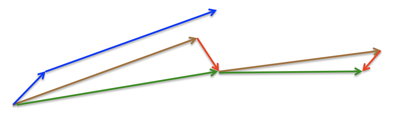
Figure 3.2: [32, lecture 6c] The blue arrow illustrates the movement of heavy ball momentum, i.e. first the small “gradient move”, then the large “momentum move”. Meanwhile the brown arrow represents the “momentum move” and the red arrow the “gradient move” for Nesterov’s momentum in green. The gradient turns around as we move towards the right, and we see that Nesterov’s momentum adjusts quicker than heavy ball momentum, which is flung outwards.

Definition 3.0.2 (Nesterov’s Momentum).

$$w_{n+1} =w_{n}+hp_{n+1},$$ (3.5a)

$$p_{n+1} =(1-hc_{f})p_{n}-h\nabla L[w_{n}+h(1-hc_{f})p_{n}]$$ (3.5b)

$$=\beta p_{n}-h\nabla L[\underbrace{w_{n}+\beta(w_{n}-w_{n-1})}_{=y_{n+1}}]$$

Discarding the momentum term and solely using the intermediate position results in the simplified version

$$w_{n+1} =y_{n+1}-\alpha\nabla\mathcal{L}(y_{n+1}),$$ (3.6a)

$$y_{n+1} =w_{n}+\beta(w_{n}-w_{n-1}).$$ (3.6b)

Dropping the intermediate position as well, results in the analog to (3.4)

$$w_{n+1} =w_{n}+\beta(w_{n}-w_{n-1})-\alpha\nabla\mathcal{L}(w_{n}+\beta(w_{n}-w_{n-1}))$$ (3.7)

Remark 3.0.3.

This method also known as “Nesterov’s Accelerated Gradient” (NAG) is said to date back to [49, in Russian]. Fortunately, [49] wrote textbooks in English, [50] (nesterovLecturesConvexOptimization2018) being the most recent. Unfortunately Chapter 2.2 on optimal methods provides barely any intuition at all, and it is advisable to consult other sources (e.g. [18]). Section 3.4 is an attempt to make these proofs somewhat intuitive.

3.1 Heavy Ball Convergence

Following the arguments from Section 1.1 in particular (1.7) we can rewrite the momentum method as

$$\begin{pmatrix}w_{n}-\hat{w}_{n}\\ w_{n+1}-\hat{w}_{n}\end{pmatrix} =\begin{pmatrix}w_{n}-\hat{w}_{n}\\ w_{n}-\hat{w}_{n}+\beta(w_{n}-w_{n-1})-\alpha\nabla\mathcal{L}^{2}(w_{n})(w_{n}-\hat{w}_{n})\end{pmatrix}$$

$$=\begin{pmatrix}0\mathbb{I}_{d}&\mathbb{I}_{d}\\ -\beta\mathbb{I}_{d}&(1+\beta)\mathbb{I}_{d}-\alpha\nabla^{2}\mathcal{L}(w_{n})\end{pmatrix}\begin{pmatrix}w_{n-1}-\hat{w}_{n}\\ w_{n}-\hat{w}_{n}\end{pmatrix}$$

For readability we will now omit the identity matrix $\mathbb{I}$ from the block matrices which are just a constant multiplied by an identity matrix. Using the digitalization of the Hessian (1.6) again, we get

$$\begin{pmatrix}0&1\\ -\beta&1+\beta-\alpha\nabla^{2}\mathcal{L}(w_{n})\end{pmatrix}$$

$$=\begin{pmatrix}V&0\\ 0&V\end{pmatrix}\begin{pmatrix}0&1\\ -\beta&\text{diag}(1+\beta-\alpha\lambda_{1},\dots,1+\beta-\alpha\lambda_{d})\end{pmatrix}\begin{pmatrix}V&0\\ 0&V\end{pmatrix}^{T}.$$

Reordering the eigenvalues from

$$\begin{pmatrix}v_{1}&\cdots&v_{d}&0&\cdots&0\\ 0&\cdots&0&v_{1}&\cdots&v_{d}\end{pmatrix}$$

to

$$\begin{pmatrix}v_{1}&0&\cdots&v_{d}&0\\ 0&v_{1}&\cdots&0&v_{d}\end{pmatrix},$$

reorders the transformation matrix of the eigenspace into a block diagonal matrix

$$R:=\begin{pmatrix}0&1\\ -\beta&1+\beta-\alpha\lambda_{1}&\\ &&\ddots&\\ &&&0&1\\ &&&-\beta&1+\beta-\alpha\lambda_{d}\\ \end{pmatrix}=:\begin{pmatrix}R_{1}\\ &\ddots\\ &&R_{d}\end{pmatrix}$$ (3.8)

So in contrast to Section 1.1, we do not get a diagonal matrix immediately. To achieve a similar eigenvalue analysis as in Section 1.1, we first have to determine the eigenvalues $r_{i1},r_{i2}$ of each $R_{i}$ and then ensure that

$$\max_{i=1,\dots,d}\max\{|r_{i1}|,|r_{i2}|\}<1.$$ (3.9)

Using the p-q formula on the characteristic polynomial of $R_{i}$ results in

$$r_{i1/2}=\tfrac{1}{2}\left(1+\beta-\alpha\lambda_{i}\pm\sqrt{(1+\beta-\alpha\lambda_{i})^{2}-4\beta}\right).$$

The analysis of these eigenvalues is very technical and can be found in the appendix. We will only cover the result here.

Figure 3.3: This is a Heat plot of $\max\{|r_{1}|,|r_{2}|\}$ for the Heavy Ball Momentum. Strictly speaking the “Monotonic” (M) and “Oscillation” (O) areas should not extend into negative $\beta$, since $r_{1/2}$ have opposite signs there. But it still describes the behavior of the dominating eigenvalue. The empty third label in the legend corresponds to the remarkably sharp border of the “Ripples” area. Drawing an actual line would have occluded the fact that it is visible by itself. Also recall that $\beta=0$ represents SGD without momentum.

Theorem 3.1.1 ([59]).

Let

$$r_{1/2}=\tfrac{1}{2}\left(1+\beta-\alpha\lambda\pm\sqrt{(1+\beta-\alpha\lambda)^{2}-4\beta}\right),$$

then

1. $\max\{|r_{1}|,|r_{2}|\}<1$ if and only if

   $$0<\alpha\lambda<2(1+\beta)\qquad\text{and}\qquad|\beta|<1.$$

2. The complex case can be characterized by either

   $$0<(1-\sqrt{\alpha\lambda})^{2}<\beta<1$$

   or alternatively $\beta>0$ and

   $$(1-\sqrt{\beta})^{2}<\alpha\lambda<(1+\sqrt{\beta})^{2},$$

   for which we have $|r_{1}|=|r_{2}|=\sqrt{\beta}$.

   As complex eigenvalues imply a rotation, this can be viewed as rotating the distance to the minimum of the quadratic function into the momentum and back like a pendulum where the friction causes it to eventually end up in the minimum. Looking at the distance to the minimum only, we will therefore observe a sinus wave (“Ripples”) as the potential energy is transferred into velocity and back. In this high momentum case convergence depends only on the amount of energy we dissipate through friction and the rate is thus equal to the square root of the momentum coefficient $\beta$ regardless of the curvature of the eigenspace.

3. In the real case we have $r_{1}>r_{2}$ and

   $$\max\{|r_{1}|,|r_{2}|\}=\begin{cases}|r_{1}|=r_{1}&\alpha\lambda<1+\beta\\ |r_{2}|=-r_{2}&\alpha\lambda\geq 1+\beta.\end{cases}$$ (3.10)

   Restricted to $1>\beta>0$ this results in two different behaviors. For

   $$0<\alpha\lambda\leq(1-\sqrt{\beta})^{2}<1+\beta,$$

   we have $1>r_{1}>r_{2}>0$ which results in a monotonic linear convergence (“Monotonic” case). For

   $$1+\beta<(1+\sqrt{\beta})^{2}\leq\alpha\lambda<2(1+\beta),$$

   on the other hand, we get $-1<r_{2}<r_{1}<0$ which implies an oscillating convergence (“Oscillation”). In contrast to the “Ripples” we switch the side of the distance to the minimum in every iteration.

Proof.

Appendix Theorem A.2.1 ∎

In particular, (positive) momentum extends the available range for learning rate and eigenvalue products $\alpha\lambda$, which results in convergence. As can be seen very well in Figure 3.3, the wider attraction area allows for moving out the largest eigenvalues to the right, with larger learning rates shifting the smaller eigenvalues towards the right as well, into more acceptable convergence rates. If the smallest and largest eigenvalues are far apart (i.e. the condition number $\kappa$ is high), this should be very useful.

So how much do we gain? In other words, what are the optimal rates of convergence?

Lemma 3.1.2 (Optimal Parameter Selection).

For a given learning rate $h$, we have

$$\min_{\beta}\max_{i=1,\dots,d}\{|r_{i1}|,|r_{i2}|\}=\max\{(1-\sqrt{\alpha\lambda_{1}}),(1-\sqrt{\alpha\lambda_{d}})\}$$

with

$$\beta^{*}=\arg\min_{\beta}\max_{i=1,\dots,d}\{|r_{i1}|,|r_{i2}|\}=\max\{(1-\sqrt{\alpha\lambda_{1}})^{2},(1-\sqrt{\alpha\lambda_{d}})^{2}\}.$$

Optimizing over the learning rate $\alpha$ as well, we get the optimal rate

$$\sqrt{\beta_{*}}=1-\frac{2}{1+\sqrt{\kappa}}.$$

for parameters

$$h_{*}=\sqrt{\alpha_{*}}=\frac{2}{\sqrt{\lambda_{1}}+\sqrt{\lambda_{d}}},\qquad\beta_{*}=\left(1-\frac{2}{1+\sqrt{\kappa}}\right)^{2}.$$

Proof.

Since the plot in Figure 3.3 looks quite symmetric, it is relatively intuitive that we only have to consider the largest and smallest eigenvalue. For now we can consider it as a lower bound:

$$\min_{\beta}\max_{i=1,\dots,d}\{|r_{i1}|,|r_{i2}|\}\geq\min_{\beta}\max_{i=1,d}\{|r_{i1}|,|r_{i2}|\}$$ (3.11)

Let us inspect the claim

$$\beta^{*}=\arg\min_{\beta}\max_{i=1,d}\{|r_{i1}|,|r_{i2}|\}=\max\{(1-\sqrt{\alpha\lambda_{1}})^{2},(1-\sqrt{\alpha\lambda_{d}})^{2}\}.$$ (3.12)

If we do select $\beta$ like this, we are still (barely) in the complex case, therefore the rate of convergence is equal to $\sqrt{\beta}$, i.e.

$$\max\{(1-\sqrt{\alpha\lambda_{1}}),(1-\sqrt{\alpha\lambda_{d}})\}.$$

Now let us wiggle around $\beta$ a bit. If we would increase $\beta$, then we are obviously increasing our rate since it is then still equal to $\sqrt{\beta}$ as we just expanded the size of the complex case. Now the question is what happens if we decrease it. By our selection of $\beta$ either the smallest or largest eigenvalue sits right at the edge of the real case. If we can show that our absolute eigenvalue maximum is increasing if we move further into the real case (decrease $\beta$), we would have proven that we can only become worse off doing so. This is annoyingly technical, so it is covered in Lemma A.2.2 in the appendix.

Now since both the largest and smallest eigenvalue are included in the complex case, we know that all eigenvalues in between must also be in the complex case which means that (3.11) is an equality proving the first two claims.

Now we have to optimize over the learning rate $\alpha$. Doing our balancing act again, only with $\sqrt{\lambda_{1}},\sqrt{\lambda_{d}}$ instead of $\lambda_{1},\lambda_{d}$, we get the same result as in (1.12), that is

$$h_{*}=\sqrt{\alpha_{*}}=\frac{2}{\sqrt{\lambda_{1}}+\sqrt{\lambda_{d}}},$$

as this makes both of them equally bad. We can plug this learning rate into either equation from inside the maximum of (3.12) to get the remaining claims about the optimal momentum $\beta_{*}$ and optimal convergence rate $\sqrt{\beta_{*}}$. ∎

This convergence rate is in fact equal to our lower bound in Theorem 1.8.4 (not even up to a constant!). So on quadratic functions we cannot do any better without violating our assumptions about possible optimizing algorithms (Assumption  1.8.5).

3.2 From Spectral Radius to Operator Norm

As the Hessian is symmetric the matrix,

$$1-h\nabla^{2}\mathcal{L}$$

is symmetric as well. And since we can find an orthonormal basis $(v_{1},\dots,v_{d})$ which diagonalizes the matrix, the operator norm is equal to the spectral radius

$$\rho(A):=\max_{i=1,\dots,d}|\lambda_{i}|,$$

for eigenvalues $\lambda_{i}$ of matrix $A$, because of

$$\|A\|=\sup_{\|x\|=1}\|Ax\|=\sup_{\|x\|=1}\sqrt{\langle Ax,Ax\rangle}=\sup_{\|x\|=1}\sqrt{\sum_{i=1}^{d}\lambda_{i}^{2}x_{i}^{2}},=\rho(A)$$

where $x=\sum_{k=1}^{d}x_{i}v_{i}$. The eigenvalue analysis was therefore sufficient for the gradient descent case

$$\|w_{n}-w_{*}\|\leq\underbrace{\|1-h\nabla^{2}\mathcal{L}\|^{n}}_{=\rho(1-h\nabla^{2}\mathcal{L})^{n}}\|w_{0}-w_{*}\|.$$

In the momentum case on the other hand, our transformation matrix $R$ (3.8) is not symmetric. But the eigenvalue analysis is still useful due to Gelfand’s Formula [24] i.e.

$$\rho(R)=\lim_{n\to\infty}\sqrt[n]{\|R^{n}\|}$$

This formula is used by [57, p. 38, Lemma 1] to argue, that we have for all $\epsilon>0$

$$\|R^{n}\|\leq\text{const }(\rho(R)+\epsilon)^{n}.$$

This still provides exponential convergence to zero for any spectral radius $\rho(R)$ smaller one. Therefore the eigenvalue analysis is still useful.

[39] already provides much tighter bounds with more explicit constants, but they still depend on the unknown quantity

$$\max_{i=1,\dots,d}\frac{\|R_{i}^{2}\|}{\|R_{i}\|^{2}}.$$

Where we can use their bounds for two dimensional matrices as the orthogonality argument still applies between blocks, so we can consider the operator norm of one block and take the maximum over all blocks

$$\|R\|=\max_{i=1,\dots,d}\|R_{i}\|=\max_{i=1,\dots,d}\left\|\begin{pmatrix}0&1\\ -\beta&1+\beta-\alpha\lambda_{i}\end{pmatrix}\right\|.$$

3.2.1 Towards Explicit Bounds

To build some intuition, notice how $\alpha\lambda_{i}=1$ and $\beta=1$ lead to

$$R_{i}=\begin{pmatrix}0&1\\ 0&0\end{pmatrix}$$

of which both eigenvalues are zero, but the operator norm is one as the vector $(0,1)^{T}$ does not change in length. Notice how we simply move the more recent weight up into the older weight slot. If we would apply the matrix again our weights would fully disappear. In other words: The problem are the cyclical eigenspaces in the jordan normal form. More precisely, we can find some basis change $U$ such that

$$R_{i}^{n}=\left(U\begin{pmatrix}r_{i1}&\delta\\ 0&r_{i2}\end{pmatrix}U^{-1}\right)^{n}=U\begin{pmatrix}r_{i1}&\delta\\ 0&r_{i2}\end{pmatrix}^{n}U^{-1}$$

where $\delta$ is zero when $r_{i1}\neq r_{i2}$ and can be zero or one if they are equal. Now if they are both equal to some value $r_{i}$, then we can write

$$\begin{pmatrix}r_{i}&\delta\\ 0&r_{i}\end{pmatrix}^{n} =\left(r_{i}\mathbb{I}+\begin{pmatrix}0&\delta\\ 0&0\end{pmatrix}\right)^{n}=\sum_{k=0}^{n}\binom{n}{k}r_{i}^{k}\begin{pmatrix}0&\delta\\ 0&0\end{pmatrix}^{n-k}$$

$$=r_{i}^{n}\mathbb{I}+nr_{i}^{n-1}\begin{pmatrix}0&\delta\\ 0&0\end{pmatrix}=\begin{pmatrix}r_{i}^{n}&\delta nr_{i}^{n-1}\\ 0&r_{i}^{n}\end{pmatrix}.$$

So together with the case $\delta=0$, we get

$$R_{i}^{n}=U\begin{pmatrix}r_{i1}^{n}&\delta nr_{i1}^{n}\\ 0&r_{i2}^{n}\end{pmatrix}U^{-1},$$

Which results in

$$\|R_{i}^{n}\| \leq\|U\|\left\|\begin{pmatrix}r_{i1}^{n}&\delta nr_{i1}^{n-1}\\ 0&r_{i2}^{n}\end{pmatrix}\right\|\|U^{-1}\|$$

$$\leq\|U\|\|U^{-1}\|\left(\left\|\begin{pmatrix}r_{i1}^{n}&0\\ 0&r_{i2}^{n}\end{pmatrix}\right\|+\delta\left\|\begin{pmatrix}0&nr_{i1}^{n-1}\\ 0&0\end{pmatrix}\right\|\right)$$

$$=\|U\|\|U^{-1}\|(\rho(R_{i})^{n}+\delta n|r_{i1}|^{n-1})$$

$$=\|U\|\|U^{-1}\|(\rho(R_{i})+\delta n)\rho(R_{i})^{n-1}$$

$$\in O(n\rho(R_{i})^{n})\subset O((\rho(R_{i})+\epsilon)^{n}).$$

Of course we do not have any bounds for $\|U\|\|U^{-1}\|$ so this is still not explicit enough. And the fact that $\delta$ jumps from zero to one (once the eigenvalues are not equal anymore) does not inspire confidence in the continuity of $U$. In fact [28, Section 7.1.5] claim that “any matrix […] that diagonalizes

$$\begin{pmatrix}1+\epsilon&1\\ 0&1-\epsilon\end{pmatrix},\qquad\epsilon\ll 1,$$

has a 2-norm condition of order $1/\epsilon$”. While this is not the same matrix, this example shows that we have to be careful. Especially since we try to select our learning rate $\alpha$ and momentum coefficient $\beta$ in such a way that we are right on the complex border (Lemma 3.1.2). So we do in fact strive for the term inside the square root to be zero

$$r_{i1/2}=\tfrac{1}{2}\left(1+\beta-\alpha\lambda_{i}\pm\sqrt{(1+\beta-\alpha\lambda_{i})^{2}-4\beta}\right),$$

and should therefore assume to be very close to $r_{i1}=r_{i2}$.

Instead of the Jordan Normal form, we therefore want to use a numerically more stable transformation, the “Schur decomposition”.

3.2.2 Schur Decomposition

Theorem 3.2.1 (Schur decomposition, [28, Theorem 7.1.3]).

If $A\in\mathbb{C}^{d\times d}$, then there exists a unitary $Q\in\mathbb{C}^{d\times d}$ such that

$$Q^{*}AQ=\text{diag}(\lambda_{1},\dots,\lambda_{d})+N$$

where $N$ is strictly upper triangular and $Q^{*}$ is the conjugate transpose of $Q$.

The neat thing about this result is, that unitary matrices are isometries for the euclidean norm.

Lemma 3.2.2 (Unitary Matrices are Isometries).

Unitary matrices $Q$ are isometries with regard to the euclidean norm

$$\|Qx\|_{2}=\|x\|_{2}\qquad\forall x\in\mathbb{C}^{d}$$

and also with regard to the induced operator norm

$$\|QA\|=\|A\|\quad\text{and}\quad\|AQ\|=\|A\|\qquad\forall A\in\mathbb{C}^{d\times d}$$

Proof.

It is straightforward to show the isometry on euclidean norms

$$\|Qx\|^{2}=\langle Qx,Qx\rangle=x^{*}Q^{*}Qx=x^{*}x=\|x\|^{2}.$$

This then translates to them being isometries for the induced operator norm on matrices, since

$$\|QA\|=\sup_{\|x\|=1}\|QAx\|=\sup_{\|x\|=1}\|Ax\|$$

and

$$\|AQ\| =\sup_{x}\frac{\|AQx\|}{\|x\|}=\sup_{x}\frac{\|AQx\|}{\|Qx\|}=\sup_{y}\frac{\|Ay\|}{\|y\|}=\|A\|.\qed$$

This lemma allows us to completely disregard the basis change matrices in our problem of estimating the operator norm of $R$. And as we are only concerned with $2\times 2$ matrices, “strictly upper triangular” still means only one entry. So we can deal with it very similarly as with the jordan normal form. The only issue is, we need to actually know the entry in the upper right corner to create an upper bound. But as it turns out, calculating the Schur decomposition for $2\times 2$ matrices is very simple. We just need one normalized eigenvector and (any of the two) normalized vectors in its orthogonal complement.

Lemma 3.2.3 (Explicit Schur Decomposition for Specific Matrix).

For a real matrix of the form

$$R=\begin{pmatrix}0&1\\ -\beta&\xi\end{pmatrix},$$

the unitary operator

$$Q:=\frac{1}{\sqrt{1+|r_{1}|^{2}}}\begin{pmatrix}1&\overline{r}_{1}\\ r_{1}&-1\end{pmatrix}$$

where $r_{1/2}=\tfrac{1}{2}\left(\xi\pm\sqrt{\xi^{2}-4\beta}\right)$ are the eigenvalues of $R$, results in the Schur Decomposition

$$Q^{*}RQ =\begin{pmatrix}r_{1}&-\frac{(1+\beta)(1+\overline{r}_{1}^{2})}{1+|r_{1}|^{2}}\\ 0&\frac{\beta\overline{r}_{1}+r_{2}}{1+|r_{1}|^{2}}\end{pmatrix}.$$

For complex eigenvalues, more specifically $4\beta\geq\xi^{2}$, we have

$$Q^{*}RQ =\begin{pmatrix}r_{1}&-(1+\overline{r}_{1}^{2})\\ 0&\overline{r}_{1}\end{pmatrix}.$$

Note that $r_{1}$ and $r_{2}$ could always be swapped to achieve a more favorable result.

Proof.

Since

$$\frac{1}{\sqrt{1+|r_{1}|^{2}}}\begin{pmatrix}1\\ r_{1}\end{pmatrix}$$

is a normalized eigenvector for eigenvalue $r_{1}$ of $R$, there are only two options of opposite direction for an orthonormal second vector

$$\pm\frac{1}{\sqrt{1+|r_{1}|^{2}}}\begin{pmatrix}-\overline{r}_{1}\\ 1\end{pmatrix},$$

which results in $Q$.

Recall that any eigenvalue of $R$, in particular $r_{1}$ and $\overline{r}_{1}\in\{r_{1},r_{2}\}$, is a root of the characteristic polynomial

$$\det(r\mathbb{I}-R)=r^{2}-r\xi+\beta=0.$$ (3.13)

With this we can calculate the Schur decomposition of $R$:

$$Q^{*}RQ =\frac{1}{1+|r_{1}|^{2}}\begin{pmatrix}1&\overline{r}_{1}\\ r_{1}&-1\end{pmatrix}\begin{pmatrix}0&1\\ -\beta&\xi\end{pmatrix}\begin{pmatrix}1&\overline{r}_{1}\\ r_{1}&-1\end{pmatrix}$$

$$=\frac{1}{1+|r_{1}|^{2}}\begin{pmatrix}1&\overline{r}_{1}\\ r_{1}&-1\end{pmatrix}\begin{pmatrix}r_{1}&-1\\ \smash{\underbrace{-\beta+\xi r_{1}}_{=r_{1}^{2}\ (\ref{eq: property of eigenvalues of R})}}&-\beta\overline{r}_{1}-\xi\end{pmatrix}\vphantom{\underbrace{\begin{pmatrix}1\\ 1\end{pmatrix}}_{=2}}$$

$$=\frac{1}{1+|r_{1}|^{2}}\begin{pmatrix}r_{1}(1+|r_{1}|^{2})&-[\beta\overline{r}_{1}^{2}+(1+\xi\overline{r}_{1})]\\ 0&\beta\overline{r}_{1}+\xi-r_{1}\end{pmatrix}$$

$$\mathrel{\smashoperator[l]{\mathop{=}_{}^{(\ref{eq: property of eigenvalues of R})}}}\begin{pmatrix}r_{1}&-\frac{\beta\overline{r}_{1}^{2}+1+(\overline{r}_{1}^{2}+\beta)}{1+|r_{1}|^{2}}\\ 0&\frac{\beta\overline{r}_{1}+\xi-r_{1}}{1+|r_{1}|^{2}}\end{pmatrix}$$

$$=\begin{pmatrix}r_{1}&-\frac{(1+\beta)(1+\overline{r}_{1}^{2})}{1+|r_{1}|^{2}}\\ 0&\frac{\beta\overline{r}_{1}+r_{2}}{1+|r_{1}|^{2}}\end{pmatrix},$$

where we have used $\xi-r_{1}=r_{2}$ in the last equation. Now in the complex case (and the case $4\beta=\xi^{2}$), we have $|r_{1}|=|r_{2}|=\sqrt{\beta}$ and $\overline{r}_{1}=r_{2}$ which results in

$$Q^{*}RQ =\begin{pmatrix}r_{1}&-(1+\overline{r}_{1}^{2})\\ 0&\overline{r}_{1}\end{pmatrix}.\qed$$

Theorem 3.2.4 (Upper Bound on Operator Norm).

Assuming our momentum coefficient is large enough but smaller one, i.e.

$$1>\beta\geq\max\{(1-\sqrt{\alpha\lambda_{1}})^{2},(1-\sqrt{\alpha\lambda_{d}})^{2}\},$$

we are in the complex case, i.e. $\rho(R)=\sqrt{\beta}$ and

$$\|R^{n}\| \leq\rho(R)^{n-1}(\rho(R)+n[1+\rho(R)^{2}])$$

$$\leq(2n+1)\rho(R)^{n-1}$$

For all $\epsilon>0$ we therefore have

$$\|R^{n}\| \leq\underbrace{\frac{3\exp(1)/\rho(R)}{\log(\rho(R)+\epsilon)-\log(\rho(R))}}_{\approx 3\exp(1)\epsilon^{-1}}[\rho(R)+\epsilon]^{n}\in O([\rho(R)+\epsilon]^{n}),\quad\forall n\geq 1$$

using the first taylor approximation

$$\log(\rho(R)+\epsilon)\approx\log(\rho(R))+\frac{\epsilon}{\log(\rho(R))}.$$

Proof.

First we apply our Lemmas to get

$$\|R^{n}\| =\max_{i=1,\dots,d}\|R_{i}^{n}\|\;\mkern-5.0mu plus -5.0mu\mathop{=}\limits^{\ref{lem: unitary matrices are isometries},\ \ref{lem: explicit schur decomposition}}\;\mkern-5.0mu plus -5.0mu\max_{i=1,\dots,d}\left\|\begin{pmatrix}r_{i1}&-(1+\overline{r}_{i1}^{2})\\ 0&\overline{r}_{i1}\end{pmatrix}^{n}\right\|.$$

Then we use Lemma A.1.6 to turn the entries into their absolute values which makes the diagonal entries equal. As the diagonal now commutes with the nilpotent matrix we can apply the binomial theorem

$$\|R^{n}\| \leq\max_{i=1,\dots,d}\Bigg{\|}\left(\begin{pmatrix}|r_{i1}|&0\\ 0&|r_{i1}|\end{pmatrix}+\begin{pmatrix}0&|1+\overline{r}_{i1}^{2}|\\ 0&0\end{pmatrix}\right)^{n}\Bigg{\|}$$

$$\leq\max_{i=1,\dots,d}\Bigg{\|}\sum_{k=0}^{n}\binom{n}{k}|r_{i1}|^{n-k}\underbrace{\left(|1+\overline{r}_{i1}^{2}|\begin{pmatrix}0&1\\ 0&0\end{pmatrix}\right)^{k}}_{=0\ \forall k>1}\Bigg{\|}$$

$$\leq\max_{i=1,\dots,d}|r_{i1}|^{n}\|\mathbb{I}\|+n|r_{i1}|^{n-1}(|1|+|r_{i1}^{2}|)\underbrace{\Bigg{\|}\begin{pmatrix}0&1\\ 0&0\end{pmatrix}\Bigg{\|}}_{=1}$$

$$\leq\max_{i=1,\dots,d}\rho(R_{i})^{n}+n\rho(R_{i})^{n-1}(1+\rho(R_{i})^{2})$$

$$=\rho(R)^{n-1}(\rho(R)+n[1+\rho(R)^{2}])$$

$$\leq\rho(R)^{n-1}(1+2n)$$

$$\leq 3n\rho(R)^{n-1}\qquad\forall n\geq 1.$$

For the second claim let $\epsilon>0$, then we have

$$\frac{\|R^{n}\|}{[\rho(R)+\epsilon]^{n}} \leq\frac{3n\rho(R)^{n-1}}{[\rho(R)+\epsilon]^{n}}$$

$$=\frac{3}{\rho(R)}\exp(\log(n)+n[\log(\rho(R))-\log(\rho(R)+\epsilon)])$$

$$\mathrel{\smashoperator[l]{\mathop{\leq}_{}^{\max_{n}}}}\frac{3}{\rho(R)}\exp\left(\log\left(\frac{1}{[\log(\rho(R)+\epsilon)-\log(\rho(R))]}\right)+1\right)$$

$$=\frac{3\exp(1)/\rho(R)}{\log(\rho(R)+\epsilon)-\log(\rho(R))}.$$

Here we simply maximized over $n$ to obtain the last inequality. ∎

3.3 Why Consider Alternatives?

While Nesterov’s Momentum breaks Assumption 1.8.5 as it uses gradients at a different point than the iterates, it does not break it fundamentally. The assumption applies to the intermediate states $y_{n}$ which are not too far from our actual iterates and would thus allow us to make similar statements about them with a bit of work.

And since heavy ball momentum can already achieve the optimal convergence rate of our complexity bounds up to some epsilon due to issues with the operator norm, why should we consider a different approach which can not be better than an already optimal method?

Weakest Link Contraction Factor

The first issue you might have noticed is: Since all eigenspaces are in the complex case, all of them have the worst contraction factor $\sqrt{\beta_{*}}$. In stochastic gradient descent on the other hand the contraction factor is $|1-h_{*}\lambda_{i}|$ for the eigenspace $i$, which can be considerably better than the worst contraction factor

$$|1-h_{*}\lambda_{d}|=|1-h_{*}\lambda_{1}|.$$

To improve the convergence rates of the worst eigenspaces we have therefore sacrificed the (possibly excellent) convergence rates of all other eigenspaces.

No General Convergence at these Rates

While [57, pp. 65-67] used the eigenvalue analysis of $\nabla\mathcal{L}^{2}(w_{*})$ to extend this rate of convergence to a local area around $w_{*}$, [41, pp. 78-79] gave an example of an $\mathcal{S}^{1,1}_{{\mu},{L}}$ function where the heavy ball method with these “optimal” parameters is trapped in an attractive cycle instead of converging.

Figure 3.4: [41]’s counterexample. Notice that the y-axis is much coarser than the x-axis and gradients are therefore much steeper than apparent. At point $-1.8$ the gradient is quite steep and the next parameter is flung across the minimum to $2.12$. Due to the less convex segment on this side, the gradient is not quite as steep here, so the iterate does not make it to the other side again which would then cause a bouncing back and forth to the minimum. Instead it stays on this side, which causes the next gradient at $0.65$ together with the built momentum in this direction to move the iterate back out to our first point.

In their counterexample from Figure 3.4, we know the parameters $\mu$ and $L$ and therefore $\alpha_{*}$ and $\beta_{*}$. They use this to explicitly write out the momentum recursion with $w_{n+1},w_{n},w_{n-1}$. Assuming a three-cycle this left them with just three linear equations which results in the three-cycle displayed in the Figure. Since we start with zero momentum, we just have to find a point to enter this cycle. Additional to solving this initialization problem, [41, pp. 93-94] show that this cycle is stable under noise (attractive).

[25] salvage some of this wreckage by proving general convergence results with tighter restrictions on hyper parameters. In particular for $\mathcal{L}\in\mathcal{S}^{1,1}_{{\mu},{L}}$ and

$$\beta\in[0,1),\qquad\alpha\in\left(0,\frac{2(1-\beta)}{L+\mu}\right)$$

they can guarantee linear convergence with an explicit, but complicated contraction factor. Notice that this is considerably weaker than the condition

$$0<\alpha\mu\leq\dots\leq\alpha L<2(1+\beta)$$

from Theorem 3.1.1. In particular momentum stops increasing the selection space for learning rates. In fact it shrinks it! This rules out rules out our optimal parameter immediately.

Similarly they prove that for $\mathcal{L}\in\mathcal{F}^{1,1}_{L}$ and

$$\beta\in[0,1),\qquad\alpha\in\left(0,\frac{(1-\beta)}{L}\right]$$

that the running minimum of loss evaluation converges to the minimal loss, with their best guarantee achieved for $\alpha=(1-\beta)/L$ resulting in

$$\min_{k=0,\dots,n}\mathcal{L}(w_{k})-\mathcal{L}(w_{*})\leq\frac{1}{1-\beta}\frac{L\|w_{0}-w_{*}\|^{2}}{2(n+1)}$$

which provides a tighter convergence bound than Theorem 1.4.1 for gradient descent without momentum $\beta=0$, but is actually harmed by momentum. While this bound might not be the best and further improvements could be made [[, see e.g.]]sunNonErgodicConvergenceAnalysis2019, it appears that we always end up with $O(1/n)$ convergence rates in the general case, which is not at all optimal, and we therefore turn towards Nesterov’s Momentum.

3.4 Nesterov’s Momentum Convergence

The Eigenvalue analysis of Nesterov’s Momentum starts out very similar, and we easily obtain the analog eigenspace transformation to (3.8)

$$R_{i}=\begin{pmatrix}0&1\\ -\beta(1-\alpha\lambda_{i})&(1+\beta)(1-\alpha\lambda_{i}).\end{pmatrix}$$

which curiously reduces to the heavy ball version if we use

$$\tilde{\beta}_{i}=\beta(1-\alpha\lambda_{i})$$ (3.14)

We therefore immediately get from Theorem 3.1.1 that $\max\{|r_{i1}|,|r_{i2}|\}<1$ if and only if

$$0<\alpha\lambda_{i}<2(1+\tilde{\beta}_{i})\quad\text{and}\quad|\tilde{\beta}_{i}|<1$$

which after some transformations is itself equivalent to

$$0<\alpha\lambda_{i}<1+\frac{1}{1+2\beta}\quad\text{and}\quad|1-\alpha\lambda_{i}|<\frac{1}{|\beta|}.$$

Figure 3.5: Heat plot of $\max\{|r_{1}|,|r_{2}|\}$ for the Nesterov Momentum. “M” and “O” stand for the “Monotonic” and “Oscillating” types of real eigenvalues. Note that the separating line of these cases $\alpha\lambda=1+\tilde{\beta}=1+\beta(1-\alpha\lambda)$ reduces to $\alpha\lambda=1$ but since we divide by $1+\beta$ the sides flip at $\beta=-1$. Again the third label is omitted to keep the remarkably sharp border unobstructed.

In a sense Nesterov’s Momentum provides every eigenspace with its own heavy ball momentum $\tilde{\beta}_{i}$ which is a good sign if we want to avoid the “Weakest Link Contraction Factor” issue we had in heavy ball momentum. And if we are in the complex case the convergence rate is $\sqrt{\beta(1-\alpha\lambda_{i})}$ which looks like the root of the gradient descent convergence rate multiplied by a factor we could make smaller than one.

As we have reduced our problem to the heavy ball problem again, we can also use the same arguments to bound the operator norm. We will therefore ignore that problem henceforth.

To ensure all eigenspaces are in the complex case, we first need to ensure that all $\tilde{\beta}_{i}$ are positive which requires

$$1-\alpha\lambda_{i}>=0$$

So let us select $\alpha=1/\lambda_{d}$. We just need to ensure that the smallest eigenvalue is in the complex case. For that, we set it to be right on the border $\tilde{\beta}_{1}=(1-\sqrt{\alpha\lambda_{1}})^{2}$, which results in

$$\beta=\frac{(1-\sqrt{\alpha\lambda_{1}})^{2}}{1-\alpha\lambda_{1}}=\frac{1-\sqrt{\alpha\lambda_{1}}}{1+\sqrt{\alpha\lambda_{1}}}=\frac{1-\sqrt{1/\kappa}}{1+\sqrt{1/\kappa}}(<1).$$

Since we have

$$\tilde{\beta}_{1}>=\dots>=\tilde{\beta}_{d}=0,$$

the worst rate of convergence is exhibited by the first eigenspace and is equal to

$$\sqrt{\tilde{\beta}_{1}}=\sqrt{(1-\sqrt{\alpha\lambda_{1}})^{2}}=1-\sqrt{1/\kappa}=1-\frac{1}{\sqrt{\kappa}}.$$ (3.15)

This rate of convergence is a tiny bit worse than the optimal heavy ball convergence rate $1-2/(1+\sqrt{\kappa})$, which is also equal to the complexity bound, but it is quite similar.

Now if you had a look at Figure 3.5 you might have noticed that for a fixed learning rate $\alpha$, the $\alpha\lambda_{i}$ are $d$ vertical lines. We made sure that the rightmost line was right on top of the black line and then moved up our momentum term until all our rates where in the ripples area. From the plot you might get the intuition that we can improve convergence if we increase the learning rate to move the largest eigenvalue into the oscillating range just like for gradient descent. And this is in fact not the optimal selection of learning rates. [41] claim, that optimal tuning results in

$$\alpha=\frac{4}{3L+\mu}\quad\text{and}\quad\beta=\frac{\sqrt{3\kappa+1}-2}{\sqrt{3\kappa+1}+2}$$

with convergence rate

$$1-\frac{2}{\sqrt{3\kappa+1}}.$$

But as we have learned with heavy ball momentum, optimal convergence rates are of no use if we cannot generalize them.

3.4.1 Estimating Sequences

To prove convergence for gradient descent, we proved that gradient descent minimizes a “local” upper bound (Lemma 1.3.1). Local in the sense that we only use the gradient information at our current position and discard all previous gradient information. To prove better convergence rates, we need to utilize the previous gradients too.

Let us start with an upper bound of the form

$$\Phi_{0}(w)=\underline{\Phi}_{0}+\tfrac{\mu_{0}}{2}\|w-z_{0}\|^{2}.$$ (3.16)

One example for such an upper bound is

$$w\mapsto\mathcal{L}(y_{0})+\langle\nabla\mathcal{L}(y_{0}),w-y_{0}\rangle+\tfrac{L}{2}\|w-y_{0}\|^{2}.$$

This is the local upper bound we minimized in Lemma 1.3.1 to obtain gradient descent. We can write this upper bound as in (3.16) with $\mu_{0}=L$, by selecting

$$z_{0}=y_{0}-L^{-1}\nabla\mathcal{L}(y_{0}).$$

Note this is the same technique as we used in (Newton-Raphson step). Also keep in mind that our upper bound is a quadratic function, which is therefore equal to its second taylor derivative.

Now since we started with an upper bound, it is trivial to find $w_{0}$ such that

$$\mathcal{L}(w_{0})\leq\min_{w}\Phi_{0}(w),$$

as we can simply select $w_{0}=z_{0}$ to get

$$\mathcal{L}(w_{0})=\mathcal{L}(z_{0})\leq\Phi_{0}(z_{0})=\min_{w}\Phi_{0}(w).$$

The idea is now, to morph our upper bound $\Phi_{0}$ via $\Phi_{n}$ slowly into a lower bound while keeping

$$\mathcal{L}(w_{n})\leq\min_{w}\Phi_{n}(w)=:\underline{\Phi}_{n}.$$ (3.17)

This would force $w_{n}$ towards the minimum as it needs to stay smaller than $\Phi_{n}$ which changes into a lower bound of $\mathcal{L}$. By controlling the speed of morphing we will be able to bound the convergence speed. But we cannot morph too fast otherwise we will not be able to stay ahead of it, i.e. fulfill (3.17).

So how do we make this concrete? The obvious lower bounds we want to utilize, are made up of all the gradients we collect along the way

$$\phi_{n}(w):=\mathcal{L}(y_{n})+\langle\nabla\mathcal{L}(y_{n}),w-y_{n}\rangle+\tfrac{\mu}{2}\|w-y_{n}\|^{2}.$$

where this includes the non strongly convex case with $\mu=0$. So let us consider

$$\Phi_{1}=\gamma\phi_{1}+(1-\gamma)\Phi_{0}$$

For $\gamma=1$ we would have a lower bound. But if $\nabla\mathcal{L}(y_{1})$ does not happen to be zero, the tangent point $y_{1}$ is sitting on a slope and is therefore not smaller than the minimum of $\phi_{1}=\Phi_{1}$. And since $\phi_{1}$ is a lower bound of $\mathcal{L}$, it will generally be impossible to satisfy (3.17) with $w_{1}$ in that case. So the first take-away is, that we can generally not select $\gamma=1$ unless we are already in the minimum. But this also hints at another issue: A convex combination of lower bounds

$$\sum_{k=0}^{n}\hat{\gamma}_{k}\phi_{k}(w)$$

is also a lower bound. But since they generally only have one tangent point which is equal and are otherwise strictly lower, it is difficult to find a $w$ such that $\mathcal{L}(w)$ is smaller than the minimum of this lower bound. So the $y_{k}$ already need to be equal to the minimum of $\mathcal{L}$ such that the $\phi_{k}$ start out with no slope and their minimum is also equal to $w_{*}$. If we have

$$\sum_{k=1}^{n}\hat{\gamma}_{k}\phi_{k}(w)+\hat{\gamma}_{0}\Phi_{0}(w)$$

we get a bit more wiggle room in the form of $\hat{\gamma}_{0}$. But if we want to slowly remove our upper bound $\Phi_{0}$, we run into a similar problem. Therefore we also need to slowly remove the old $\phi_{k}$ upper bounds, constructed with $y_{k}$ far away from the minimum $w_{*}$. This motivates why we might wish to select

$$\Phi_{n}(w):=\gamma_{n}\phi_{n}(w)+(1-\gamma_{n})\Phi_{n-1}(w)$$ (3.18)

causing an exponential decay not only for the initial upper bound, but also for our previous lower bounds. For

$$\Gamma_{k}^{n}:=\prod_{i=k}^{n}(1-\gamma_{i})$$

one can inductively convert the recursion (3.18) into

$$\Phi_{n}(w) =\sum_{k=1}^{n}\Gamma_{k+1}^{n}\gamma_{k}\phi_{k}(w)+\Gamma_{1}^{n}\Phi_{0}(w)$$

$$\leq(1-\Gamma_{1}^{n})\mathcal{L}(w)+\Gamma_{1}^{n}\Phi_{0}(w)$$ (3.19)

Lemma 3.4.1.

If the $w_{n}$ satisfy (3.17), then we have

$$\mathcal{L}(w_{n})-\mathcal{L}(w_{*})\leq\Gamma_{1}^{n}(\Phi_{0}(w_{*})-\mathcal{L}(w_{*})).$$

This motivates why we are interested in $\Gamma_{1}^{n}\to 0$. A sufficient condition is

$$\sum_{k=0}^{\infty}\gamma_{k}=\infty$$

Proof.

Both statements are fairly easy to prove:

$$\mathcal{L}(w_{n})\;\mkern-5.0mu plus -5.0mu\mathop{\leq}\limits^{(\ref{eq: staying ahead of the estimates})}\;\mkern-5.0mu plus -5.0mu\min_{w}\Phi_{n}(w) \mathrel{\smashoperator[l]{\mathop{\leq}_{}^{(\ref{eq: estimating sequence explicit})}}}\min_{w}\{(1-\Gamma_{1}^{n})\mathcal{L}(w)+\Gamma_{1}^{n}\Phi_{n}(w)\}$$

$$\leq(1-\Gamma_{1}^{n})\mathcal{L}(w_{*})+\Gamma_{1}^{n}\Phi_{n}(w_{*})$$

Subtracting $\mathcal{L}(w_{*})$ from both sides lets us move on to the second statement:

$$\Gamma_{1}^{n} =\prod_{i=1}^{n}(1-\gamma_{i})\leq\prod_{i=1}^{n}\exp(-\gamma_{i})=\exp\left(-\sum_{i=1}^{n}\gamma_{i}\right)\to 0\qed$$

Now we just need to make sure that we can actually satisfy (3.17) while making $\gamma_{k}$ as large as possible. For gradient descent we just minimized the quadratic upper bound $\Phi_{0}$. Now we need to minimized the $\Phi_{n}$. For that we want an explicit representation of $\Phi_{n}$. Fortunately we are only adding up quadratic functions, therefore the function $\Phi_{n}$ is quadratic too, and can thus be written in the form

$$\Phi_{n}(w)=\underline{\Phi}_{n}+\tfrac{\mu_{n}}{2}\|w-z_{n}\|^{2},$$ (3.20)

where $z_{n}$ is the minimum, and our convexity parameter $\mu_{n}$ morphs from $\mu_{0}$ to $\mu$

$$\mu_{n}=(1-\Gamma_{1}^{n})\mu+\Gamma_{1}^{n}\mu_{0}=\gamma_{n}\mu+(1-\gamma_{n})\mu_{n-1},$$ (3.21)

because $\mu_{n-1}\mathbb{I}$ is by induction the Hessian of $\Phi_{n}$. Assuming (3.17) holds for $n-1$, we can write our minimal value as

$$\underline{\Phi}_{n} =\Phi_{n}(y_{n})-\tfrac{\mu_{n}}{2}\|y_{n}-z_{n}\|^{2}$$

$$\mathrel{\smashoperator[l]{\mathop{=}_{}^{(\ref{eq: estimating sequence recursion})}}}\gamma_{n}\underbrace{\phi_{n}(y_{n})}_{=\mathcal{L}(y_{n})}+(1-\gamma_{n})\underbrace{\Phi_{n-1}(y_{n})}_{=\underbrace{\underline{\Phi}_{n-1}}_{\geq\mathcal{L}(w_{n-1})\mathrlap{\geq\mathcal{L}(y_{n})+\langle\mathcal{L}(y_{n}),w_{n-1}-y_{n}\rangle}}+\mathrlap{\tfrac{\mu_{n-1}}{2}\|y_{n}-z_{n-1}\|^{2}}}-\tfrac{\mu_{n}}{2}\|y_{n}-z_{n}\|^{2}$$

$$\geq\mathcal{L}(y_{n})+\text{``junk''}\;\mkern-5.0mu plus -5.0mu\mathop{\geq}\limits^{?}\;\mkern-5.0mu plus -5.0mu\mathcal{L}(y_{n})-\tfrac{1}{2L}\|\nabla\mathcal{L}(y_{n})\|^{2}$$

Now you might recall that $y_{n}$ are our intermediate “information collection points”, which then define the actual iterate. And since Lemma 1.3.1, we know that we can achieve

$$\mathcal{L}(y_{n})-\tfrac{1}{2L}\|\nabla\mathcal{L}(y_{n})\|^{2}\geq\mathcal{L}(w_{n})$$

by selecting the learning rate $\alpha=1/L$ in

$$w_{n}=y_{n}-\alpha\nabla\mathcal{L}(y_{n}).$$

To be able to satisfy (3.17), we therefore only need to lower bound our “junk”

$$J:=(1-\gamma_{n})\left(\langle\mathcal{L}(y_{n}),w_{n-1}-y_{n}\rangle+\tfrac{\mu_{n-1}}{2}\|y_{n}-z_{n-1}\|^{2}\right)-\tfrac{\mu_{n}}{2}\|y_{n}-z_{n}\|^{2}$$

by $-\tfrac{1}{2L}\|\nabla\mathcal{L}(y_{n})\|^{2}$. By having a closer look at $z_{n}$ and expressing it in terms of $z_{n-1}$, the necessary terms fall out and we obtain the following sufficient conditions

Lemma 3.4.2 (Dumpster Dive).

The conditions

$$L\gamma_{n}^{2}\leq\mu_{n}\;\mkern-5.0mu plus -5.0mu\mathop{=}\limits^{\text{def.}}\;\mkern-5.0mu plus -5.0mu\gamma_{n}\mu+(1-\gamma_{n})\mu_{n-1}\qquad\forall n\geq 1$$ (3.22a)

or equivalently for $$\kappa_{n}:=L/\mu_{n}$$

$$\gamma_{n}^{2} \leq\gamma_{n}\kappa^{-1}+(1-\gamma_{n})\kappa_{n-1}^{-1}\qquad\forall n\geq 1$$ (3.22b)

and

$$y_{n} =\frac{\mu_{n}w_{n-1}+\mu_{n-1}\gamma_{n}z_{n-1}}{\gamma_{n}\mu+\mu_{n-1}}$$ (3.23)

are sufficient for $J\geq-\tfrac{1}{2L}\|\nabla\mathcal{L}(y_{n})\|^{2}$.

Proof.

See Appendix Lemma A.2.3. ∎

As we are allowed to select $\gamma_{n}$ and $y_{n}$ in iteration $n$ we can ensure that these equations are in fact fulfilled.

3.4.2 Convergence Results

Now while $\Phi_{0}$ being an upper bound was nice to build intuition, we do not actually need it to be an upper bound. The only thing we really need is for equation (3.17) and (3.20) to hold for $n=0$ so that we can do our induction. In particular picking any $w_{0}$ and selecting

$$\Phi_{0}(w):=\mathcal{L}(w_{0})+\tfrac{\mu}{2}\|w_{0}-w\|^{2}$$

works as well. And in that case we have $\mu_{n}=\mu$ for all $n$, which simplifies (3.22b) to

$$\gamma_{n+1}=\frac{1}{\sqrt{\kappa}}\implies\Gamma_{1}^{n}=(1-\tfrac{1}{\sqrt{\kappa}})^{n}.$$ (3.24)

With Lemma 3.4.1 in mind this hints at how we get our convergence rate (3.15) we derived with eigenvalues back! But since $\mu=0$ implies $\kappa=\infty$, which would set our rate of convergence to one, we will continue to entertain the general case with general $\mu_{0}$ summarized in Algorithm 1.

Input: starting point $w_{0}$, and some $\mu_{0}>0$

1 $z_{0}\leftarrow w_{0}$; $n\leftarrow 1$;

2 while not converged do

Select $\gamma_{n}\in(0,1)$ such that

   $$L{\gamma }_n^2={\gamma }_n\mu +\left(1-{\gamma }_n\right){\mu }_{n-1};$$ 3

4    

5     $\mu_{n}\leftarrow\gamma_{n}\mu+(1-\gamma_{n})\mu_{n-1}$

6    

7    $y_{n}\leftarrow\displaystyle\frac{\mu_{n}w_{n-1}+\mu_{n-1}\gamma_{n}z_{n-1}}{\gamma_{n}\mu+\mu_{n-1}}$

8    

Select $w_{n}$ such that // e.g. $w_{n}=y_{n}-\tfrac{1}{L}\nabla\mathcal{L}(y_{n})$ (Lem 1.3.1)

   $$ℒ\left(w_n\right)\le ℒ\left(y_n\right)-\frac{1}{2L}{\Vert \nabla ℒ\left(y_n\right)\Vert }^2$$ 9

10    

     $z_{n}\leftarrow\tfrac{1}{\mu_{n}}\left[\gamma_{n}\mu y_{n}+(1-\gamma_{n})\mu_{n}z_{n-1}-\gamma_{n}\nabla\mathcal{L}(y_{n})\right]$

      // (A.9)

11    

12    $n\leftarrow n+1$

13    

14 end while

Algorithm 1 General Schema of Optimal Methods (by [50])

Figure 3.6 visualizes how larger $\mu_{0}$ than $\mu$ increase the $\gamma_{n}$ to be larger than zero and thus decrease the $\Gamma_{1}^{n}$ below one. It also explains why we should make (3.22a) an equality.

Figure 3.6: Picking the largest possible $\gamma_{n}$ which satisfy (3.22b) makes the inequality an equality $L\gamma_{n}^{2}=\mu_{n}$, and therefore $\kappa_{n}^{-1}=\gamma_{n}^{2}$. If we start out with $\kappa_{0}=\kappa$, we therefore have $\gamma_{n}=\hat{\gamma}=\sqrt{\kappa^{-1}}$ for all $n$. In all other cases $\hat{\gamma}$ still acts as an attraction point. For $\kappa^{-1}=0$ i.e. $\mu=0$ we see how it might be helpful to select a different $\kappa_{0}$ even though increasing $\mu_{0}$ (i.e. $\kappa_{0}^{-1}$) increases $\Phi_{0}$ which is part of the bound on convergence.

Before we address convergence rates for general $\mu_{0}$ let us take a closer look at the strange looking $y_{n+1}$, which were much more simple in Definition 3.0.2 and try to get rid of additional baggage like $z_{n}$ and $\mu_{n}$.

Lemma 3.4.3.

If we use the recursion

$$w_{n}=y_{n}-\tfrac{1}{L}\mathcal{L}(y_{n})$$ (3.25)

in Algorithm 1 line 1, then we can simplify $z_{n}$ and $y_{n}$ to

$$z_{n} =w_{n-1}+\tfrac{1}{\gamma_{n}}(w_{n}-w_{n-1})\qquad\forall n\geq 1$$ (3.26)

$$y_{n+1} =w_{n}+\beta_{n}(w_{n}-w_{n-1})\qquad\forall n\geq 0$$ (3.27)

for $w_{-1}:=w_{0}=z_{0}$ and

$$\beta_{n}=\frac{\mu_{n}\gamma_{n+1}(1-\gamma_{n})}{\gamma_{n}(\gamma_{n+1}\mu+\mu_{n})}=\frac{\gamma_{n}(1-\gamma_{n})}{\gamma_{n}^{2}+\gamma_{n+1}}$$ (3.28)

Proof.

See Appendix Lemma A.2.4 ∎

With the streamlined recursion from Lemma 3.4.3 we only need $\mu_{n}$ for the recursion of $\gamma_{n+1}$ itself at this point. So we can now use the equivalent recursion (3.22b) with $\kappa_{n}:=L/\mu_{n}$. By defining $\gamma_{0}:=1/\sqrt{\kappa_{0}}$ we can ensure

$$\gamma_{n}^{2}=\kappa_{n}^{-1}\qquad\text{for all }n\geq 0.$$

This in turn allows us to get rid of the $\kappa_{n}$. Applying the p-q formula and discarding the negative option, results in the explicit recursion

$$\gamma_{n+1}=\tfrac{1}{2}\left[-(\gamma_{n}^{2}-\kappa^{-1})+\sqrt{(\gamma_{n}^{2}-\kappa^{-1})^{2}+4\gamma_{n}^{2}}\right].$$

Since we get a fixed $\hat{\gamma}=1/\sqrt{\kappa}$ for $\mu_{0}=\mu$, the momentum coefficient is fixed in this case and equal to

$$\hat{\beta}=\frac{1-1/\sqrt{\kappa}}{1+1/\sqrt{\kappa}}$$

which we recognize from our eigenvalue analysis.

Input: starting point $w_{0}$, and some $\kappa_{0}>0$

$\gamma_{0}\leftarrow 1/\sqrt{\kappa_{0}}$

  // $\gamma_{n}^{2}=\kappa_{n}^{-1}$ in (3.22b) makes $\kappa_{n}$ obsolete

1 $w_{-1}\leftarrow w_{0}$

2 $n\leftarrow 0$

3 while not converged do

4     $\gamma_{n+1}\leftarrow\tfrac{1}{2}\left[(\kappa^{-1}-\gamma_{n}^{2})+\sqrt{(\kappa^{-1}-\gamma_{n}^{2})^{2}+4\gamma_{n}^{2}}\right]$

     // $=1/\sqrt{\kappa}$ if $\kappa_{0}=\kappa$

5    

    $\beta_{n}\leftarrow\displaystyle\frac{\gamma_{n}(1-\gamma_{n})}{\gamma_{n+1}+\gamma_{n}^{2}}$

      // $=\frac{1-1/\sqrt{\kappa}}{1+1/\sqrt{\kappa}}$ if $\kappa_{0}=\kappa$

6    

    $y_{n+1}\leftarrow w_{n}+\beta_{n}(w_{n}-w_{n-1})$

      // $\beta_{0}$ does not matter!

7    

8    $w_{n+1}\leftarrow y_{n+1}-\tfrac{1}{L}\nabla\mathcal{L}(y_{n+1})$

9    

10    $n\leftarrow n+1$

11    

12 end while

Algorithm 2 Dynamic Nesterov Momentum

What is left to do is an analysis of convergence, in particular for the case where $\kappa_{0}\neq\kappa$, which is especially applicable for $\mu=0$. Figure 3.6 provides some intuition why it might also be useful to have $\kappa_{0}>\kappa$ when $\mu\neq 0$.

Theorem 3.4.4.

Let $\mathcal{L}\in\mathcal{S}^{1,1}_{{\mu},{L}}$ (includes $\mathcal{L}\in\mathcal{F}^{1,1}_{L}$ with $\mu=0$). For starting point $w_{0}$ and some $\kappa_{0}$ (equivalently $\mu_{0}$ or $\gamma_{0}$) let $w_{n}$ be selected via Algorithm 1 or 2, then for $\Gamma^{n}:=\Gamma_{1}^{n}=\prod_{k=1}^{n}(1-\gamma_{k})$ we have

$$\mathcal{L}(w_{n})-\mathcal{L}(w_{*}) \leq\Gamma^{n}\left[\mathcal{L}(w_{0})-\mathcal{L}(w_{*})+\tfrac{\mu_{0}}{2}\|w_{0}-w_{*}\|^{2}\right]$$

$$\leq\Gamma^{n}\tfrac{L+\mu_{0}}{2}\|w_{0}-w_{*}\|^{2}$$

where we have for $\kappa_{0}^{-1}\in(\kappa^{-1},3+\kappa^{-1}]$

$$\Gamma^{n}\leq\frac{4\kappa^{-1}}{(\kappa_{0}^{-1}-\kappa^{-1})\left[\exp\left(\frac{n+1}{2\sqrt{\kappa}}\right)-\exp\left(-\frac{n+1}{2\sqrt{\kappa}}\right)\right]^{2}}\leq\frac{4}{(\kappa_{0}^{-1}-\kappa^{-1})(n+1)^{2}}$$

and for $\kappa_{0}=\kappa$

$$\Gamma^{n}=(1-\sqrt{\kappa^{-1}})^{n}\leq\exp\left(-\frac{n}{\sqrt{\kappa}}\right)$$

Proof.

We can use

$$\Phi_{0}(w):=\mathcal{L}(w_{0})+\tfrac{\mu_{0}}{2}\|w-w_{0}\|^{2}$$

to ensure $w_{0}=z_{0}$ for Lemma 3.4.3 needed for Algorithm 2. We can then apply Lemma 3.4.1 to obtain

$$\mathcal{L}(w_{n})-\mathcal{L}(w_{*}) \leq\Gamma_{1}^{n}(\Phi_{0}(w_{*})-\mathcal{L}(w_{*}))$$

$$=\Gamma^{n}\left[\mathcal{L}(w_{0})-\mathcal{L}(w_{*})+\tfrac{\mu_{0}}{2}\|w_{0}-w_{*}\|^{2}\right].$$

We can bound the original loss with the weight difference (Lemma 1.2.4)

$$\mathcal{L}(w_{0})-\mathcal{L}(w_{*})\leq\tfrac{L}{2}\|w_{0}-w\|^{2}$$

to get the second upper bound. Now to the upper bound on $\Gamma^{n}$. We have already covered the case $\kappa_{0}=\kappa$ in (3.24), (with $1+x\leq\exp(x)$ in mind). The general case is covered in the Lemma A.2.5 ∎

3.5 Hyperparameter Selection

Knowing the condition number, one might wish to optimize the convergence rate of Theorem 3.4.4 over $\kappa_{0}$. For $\kappa_{0}^{-1}\in(\kappa^{-1},3+\kappa^{-1}]$ this entails minimizing

$$\frac{L+\mu_{0}}{\kappa_{0}^{-1}-\kappa^{-1}}=L\frac{1+\kappa_{0}^{-1}}{\kappa_{0}^{-1}-\kappa^{-1}}=L\frac{1+\frac{1}{\kappa_{0}^{-1}}}{1-\frac{\kappa^{-1}}{\kappa_{0}^{-1}}}$$ (3.29)

Since both, the enumerator decreases with $\kappa_{0}^{-1}$, and the denominator increases with $\kappa_{0}^{-1}$, we want to select $\kappa_{0}^{-1}$ as large as possible.

Looking at Figure 3.6 this should make us suspicious. There is nothing special about $\kappa_{0}^{-1}=3+\kappa^{-1}$ when it comes to $\Gamma^{n}$. The $\gamma_{n}$ are still increasing afterwards. And from (3.29) it seems that the trade-off of higher $\mu_{0}$ seems to be worth it. So maybe we should have another go at bounding $\Gamma^{n}$. But instead of diving head first into even more technical calculations, we could also consider the fact that

$$\Gamma^{n}=\prod_{k=1}^{n}(1-\gamma_{k})=(1-\gamma_{1})\Gamma_{2}^{n}$$

and simply use Lemma A.2.5 with $\tilde{\gamma}_{k}=\gamma_{k+1}$ to bound $\Gamma_{2}^{n}=\tilde{\Gamma}^{n-1}$ using the fact that

$$\tilde{\kappa}_{0}^{-1}=\kappa_{1}^{-1}=\gamma_{1}^{2}\leq 1\leq 3+\kappa^{-1}.$$

With this trick we get

$$\Gamma^{n} \leq\frac{4\kappa^{-1}(1-\gamma_{1})}{(\gamma_{1}^{2}-\kappa^{-1})\left[\exp\left(\frac{n}{2\sqrt{\kappa}}\right)-\exp\left(-\frac{n}{2\sqrt{\kappa}}\right)\right]^{2}}\leq\frac{4(1-\gamma_{1})}{(\gamma_{1}^{2}-\kappa^{-1})n^{2}}.$$

With Theorem 3.4.4 the relevant constant to optimize is

$$\frac{4(1-\gamma_{1})}{\gamma_{1}^{2}-\kappa^{-1}}\frac{L+\mu_{0}}{2}=\frac{2(1-\gamma_{1})}{\gamma_{1}^{2}-\kappa^{-1}}(1+\kappa_{0}^{-1})L$$

and we can use the $\gamma_{n}$ recursion (3.22b) to rewrite $\kappa_{0}^{-1}$ as

$$\kappa_{0}^{-1}=\frac{\gamma_{1}^{2}-\gamma_{1}\kappa^{-1}}{1-\gamma_{1}}.$$

Using this representation we want to minimize

$$c(\gamma_{1}):=2L\frac{(1-\gamma_{1})+(\gamma_{1}^{2}-\gamma_{1}\kappa^{-1})}{\gamma_{1}^{2}-\kappa^{-1}}\qquad\gamma_{1}\in(\sqrt{\kappa^{-1}},1).$$

By taking the derivative of $c$ one can show that it is monotonously decreasing (Lemma A.2.6). Taking $\gamma_{1}=1$ would imply an infinite $\kappa_{0}^{-1}$ (and $\mu_{0}$) and therefore seems to prevent us from doing so at first glance, but all relevant things like the loss difference upper bound

$$\mathcal{L}(w_{n})-\mathcal{L}(w_{*})\leq c(\gamma_{1})\frac{\kappa^{-1}\|w_{0}-w_{*}\|^{2}}{\left[\exp\left(\frac{n}{2\sqrt{\kappa}}\right)-\exp\left(-\frac{n}{2\sqrt{\kappa}}\right)\right]^{2}}\leq c(\gamma_{1})\frac{\|w_{0}-w_{*}\|}{n^{2}},$$ (3.30)

the momentum $\beta_{n}$ (except for $\beta_{0}$ which does not matter) and our weight iterates $w_{n}$ are continuous in $\gamma_{1}$ at one. The limit

$$c(1)=2L$$

is therefore reasonable.

Input: starting point $w_{0}$ (condition number $\kappa$, lipschitz constant $L$)

1 $y_{1}\leftarrow w_{0}$

2 $w_{1}\leftarrow y_{1}-\tfrac{1}{L}\nabla\mathcal{L}(y_{1})$

3

4$\gamma_{1}\leftarrow 1$; $n\leftarrow 1$

5 while not converged do

6     $\gamma_{n+1}\leftarrow\tfrac{1}{2}\left[(\kappa^{-1}-\gamma_{n}^{2})+\sqrt{(\kappa^{-1}-\gamma_{n}^{2})^{2}+4\gamma_{n}^{2}}\right]$

7    

8    $\beta_{n}\leftarrow\displaystyle\frac{\gamma_{n}(1-\gamma_{n})}{\gamma_{n+1}+\gamma_{n}^{2}}$

9    

10    $y_{n+1}\leftarrow w_{n}+\beta_{n}(w_{n}-w_{n-1})$

11    

12    $w_{n+1}\leftarrow y_{n+1}-\tfrac{1}{L}\nabla\mathcal{L}(y_{n+1})$

13    

14    $n\leftarrow n+1$

15    

16 end while

Algorithm 3 Optimal Nesterov Momentum

Corollary 3.5.1.

For $\mathcal{L}\in\mathcal{S}^{1,1}_{{\mu},{L}}$ (includes $\mathcal{L}\in\mathcal{F}^{1,1}_{L}$ with $\mu=0$), $w_{n}$ selected by Algorithm 3 we get

$$\mathcal{L}(w_{n})-\mathcal{L}(w_{*})\leq\frac{2\mu\|w_{0}-w_{*}\|^{2}}{\left[\exp\left(\frac{n}{2\sqrt{\kappa}}\right)-\exp\left(-\frac{n}{2\sqrt{\kappa}}\right)\right]^{2}}\leq\frac{2L\|w_{0}-w_{*}\|}{n^{2}},$$

where the term in the middle should be ignored for $\mu=0$.

Proof.

Plugging $c(1)=2L$ into (3.30). ∎

3.5.1 Practical Hyperparameter Selection

While Algorithm 3 eliminates another hyperparameter, we still need to somehow know the Lipschitz constant $L$ of the gradient and the condition number $\kappa$.

The Lipschitz constant can be estimated with Backtracking (Section 1.7). With the condition number we could just be conservative and set $\kappa^{-1}=0$. This sacrifices linear convergence, but in view of the asymptotic convergence rates stochasticity causes, this might not be so bad. But in situations where the “transient phase” (before stochasticity kills fast progression) is significant, this might not be a satisfactory answer.

Figure 3.7: Since momentum $\beta_{n}$ is a function of $(\gamma_{n},\gamma_{n+1})$, and $\gamma_{n+1}$ is a function of $(\gamma_{n},\kappa^{-1})$, momentum can be viewed as a function of $(\gamma,\kappa^{-1})$. This function $\beta(\gamma,\kappa^{-1})$ is plotted here over $\gamma$ for different $\kappa^{-1}$. Since the sequence of $\gamma_{n}$ stays above $\hat{\gamma}=\sqrt{\kappa^{-1}}$ the line is dotted below this threshold.

From our eigenvalue analysis, we know that smaller eigenvalues will generally still converge (even if we neglect them) although at a slower rate. So we could just guess a condition and see how it goes. And if we have a look at Figure 3.7 a condition guess will simply stop the progression of $\gamma_{n}$ towards zero at this point and consequently stop the progression of $\beta_{n}$ towards one. If we dislike the resulting convergence speed, we can probably just increase the condition number on the fly which causes the $\gamma_{n}$ to fall further and momentum to continue its move towards one. In Figure 3.8 we can see that it only takes very few iterations until we converge to $\hat{\beta}=\frac{1-\sqrt{\kappa^{-1}}}{1+\sqrt{\kappa^{-1}}}$ if $\kappa^{-1}>0$.

Figure 3.8: Starting from $\gamma_{1}=1$ the progression of $\beta_{n}$ for different condition numbers $\kappa$. The heuristics $\beta_{n}=\frac{t_{n}-1}{t_{n+1}}$ where $t_{1}=1$ and $t_{n}=\tfrac{1}{2}(1+\sqrt{1+4t_{n}^{2}})$ and $\beta_{n}=\frac{n-1}{n+2}$ seem to be popular in practice [61].

What we can also see in Figure 3.8 is that

$$\beta_{n}=\frac{n-1}{n+2}=1-\frac{3}{n+2}$$ (3.31)

is a decent approximation for the $\beta_{n}$ progression when $\kappa^{-1}=0$. If we recall our original motivation, $\beta$ was $1-hc_{f}$ where $c_{f}$ was a friction parameter. [71] show that in the limit of $h\to 0$, nesterov momentum with momentum coefficient (3.31) approximates the differential equation

$$\ddot{w}+\frac{3}{t}\dot{w}+\nabla\mathcal{L}(w)=0$$

i.e. decreasing friction $c_{f}=3/t$ over time. They then use this continuous approximation to derive better convergence rates ($O(1/n^{3})$ instead of $O(1/n^{2})$) when this conservative ($\kappa^{-1}=0$) assumption is used, but the loss function is strongly convex. They also propose a scheme of “restarting” Nesterov’s Momentum to achieve linear convergence in the strongly convex case without knowing the condition number (a restart effectively resets momentum back to a lower level).

Last but not least recall that $\alpha=1/L$ is the squared discretization $h^{2}$ of the ODE which can deceive you into thinking that the discretization is similar given that gradient descent converges for $h\in(0,2/L)$. But the implied discretization $h=1/\sqrt{L}$ of Nesterov’s Momentum is much larger in general. This provides some intuition for where the speedup comes from.

3.6 Stochasticity

It has not yet fully crystalized whether or not Momentum is beneficial in a stochastic setting. Since movement is determined by the integral (sum) of gradients in this setting, one can argue intuitively, that we might get a sort of averaging effect, which should reduce variance and be beneficial for convergence [[, e.g.]p. 69]bottouOptimizationMethodsLargeScale2018. [26] on the other hand claim that “increasing momentum, contrary to popular belief, causes the errors to compound”, most likely citing [17].

Now as we can already achieve optimal performance (in the BLUE sense) for variance reduction in SGD (cf. Subsection 2.2.1), it is also intuitive why momentum might not be beneficial in stochastic settings. But since it simply introduces additional parameters ($\beta$ could be zero to get GD again), it provides a bit more freedom to play with. [21] show that this freedom in parameters results in a close relation of momentum to the averaging GD, which we have discussed in Section 2.5.

Chapter 4 Other Methods

4.1 Heuristics for Adaptive Learning Rates

There are a number of widely used heuristics which are provided in the default optimizer selection of machine learning frameworks such as Tensorflow.

As we have only covered gradient descent and momentum so far, we have quite a bit of ground to cover. But at the same time most of the remaining common optimizers [[, as reviewed by e.g.]]ruderOverviewGradientDescent2017 can be motivated in a similar way, which might or might not be new.

Recall that the Newton-Raphson step

$$w_{n+1}=w_{n}-(\nabla^{2}\mathcal{L}(w_{n}))^{-1}\nabla\mathcal{L}(w_{n})$$

finds the vertex of a quadratic loss function $\mathcal{L}$ immediately, because we have

$$\nabla\mathcal{L}(w_{n})=\nabla^{2}\mathcal{L}(w_{n})[w_{n}-\hat{w}_{n}],$$

where $\hat{w}_{n}$ was the vertex of the second Taylor approximation. To better understand how that works, note that for

$$\nabla^{2}\mathcal{L}(w_{n})=V\text{diag}(\lambda_{1},\dots,\lambda_{d})V^{T}$$

we have

$$\nabla^{2}\mathcal{L}(w_{n})^{-1}=V\text{diag}(\tfrac{1}{\lambda}_{1},\dots,\tfrac{1}{\lambda}_{d})V^{T}.$$

To simplify things, let us assume a quadratic loss function $H=\nabla^{2}\mathcal{L}(w_{n})$ now. In this case we found that every eigenspace scales independently

$$\langle w_{n+1}-w_{*},v_{i}\rangle\leq(1-h\lambda_{i})\langle w_{n}-w_{*},v_{i}\rangle.$$

The Newton-Raphson step rescales these steps by dividing every eigenspace through its respective eigenvalue. For positive eigenvalues this is all nice and dandy. But for negative eigenvalues, which represent a maximum in their eigenspace, the Newton-Raphson step multiplies the gradient by a negative value $\tfrac{1}{\lambda_{i}}$ and therefore causes movement towards this eigenvalue.

Okay, now that we remembered these crucial problems, let us make one egregious assumption. Let us assume that the standard basis are already the eigenvectors, i.e. $V=\mathbb{I}$. Then the components of the gradient of our loss function are proportional to their respective eigenvalues

$$\nabla\mathcal{L}(w_{n})^{(i)}=\lambda_{i}[w_{n}-w_{*}]^{(i)}.$$

If we define

$$G_{n}^{(i)}=\sum_{k=0}^{n}[\nabla\mathcal{L}(w_{n})^{(i)}]^{2}\qquad i=1,\dots,d,$$

then the algorithm

$$w_{n+1}^{(i)} =w_{n}^{(i)}-\frac{h_{n}}{\sqrt{G_{n}^{(i)}}}\nabla\mathcal{L}(w_{n})^{(i)}$$ (4.1)

$$=w_{n}^{(i)}-\frac{h_{n}}{\sqrt{\cancel{\lambda_{i}^{2}}\sum_{k=0}^{n}([w_{k}-w_{*}]^{(i)})^{2}}}\cancel{\lambda_{i}}[w_{n}-w_{*}]^{(i)}$$

also cancels out the eigenvalues. But as we divide through the absolute value of the eigenvalues in contrast to the Newton-Raphson step, we get to keep the sign

$$[w_{n+1}-w_{*}]^{(i)}=\left(1-\frac{h_{n}\text{sign}(\lambda_{i})}{\sqrt{\sum_{k=0}^{n}([w_{k}-w_{*}]^{(i)})^{2}}}\right)[w_{n}-w_{*}]^{(i)}.$$ (4.2)

Of course the notion that the standard basis vectors are already the eigenvectors is pretty ridiculous. But for some reason the following algorithms seem to work. And they are based on this notion of reweighting the components by dividing them through the squared past gradients in some sense. The intuition provided by [63] is, that “It adapts the learning rate to the parameters, performing smaller updates (i.e. low learning rates) for parameters associated with frequently occurring features, and larger updates (i.e. high learning rates) for parameters associated with infrequent features.” But even this intuition seems to assume that these “features” somehow correspond to the coordinates vectors.

AdaGrad

[20] We have already motivated most of AdaGrad in (4.1). But we will use the stochastic gradients

$$G_{n}^{(i)}:=\sum_{k=0}^{n}[\nabla l(w_{n},Z_{n})^{(i)}]^{2}\qquad i=1,\dots,d,$$

and introduce a small term $\epsilon$ [[, $\approx 10^{-8}$]]ruderOverviewGradientDescent2017 to avoid numerical instability (see also Levenberg-Marquard regularization, Subsection 4.5.2). This results in the “AdaGrad” algorithm

$$W_{n+1}^{(i)} =W_{n}^{(i)}-\frac{h_{n}}{\sqrt{G_{n}^{(i)}+\epsilon}}\nabla l(W_{n},Z_{n})^{(i)}\qquad i=1,\dots,d.$$

If we were to divide the sum of squared gradients $G_{n}^{(i)}$ by the number of summands, we would get an estimator for the second moment. This second moment consists not only of the average squares of the actual loss function, but also of a variance estimator. This means that high variance can also reduce the learning rate. This is an additional benefit, as we have found when looking at SGD, that we need to reduce the learning rate when the variance starts to dominate.

RMSProp

[32, lecture 6e] As the sum of squares increases monotonically, we can see in (4.2) that this quickly reduces the learning rate of AdaGrad in every step. So RMSProp actually uses an estimator for the second moments, i.e. divides $G_{n}^{(i)}$ by $n$. Well, that is a bit of a lie. To avoid calculations it uses a recursive exponential average

$$\hat{\mathbb{E}}[(\nabla l(W_{n})^{(i)})^{2}]:=\gamma\hat{\mathbb{E}}[(\nabla l(W_{n-1})^{(i)})^{2}]+(1-\gamma)(\nabla l(W_{n},Z_{n})^{(i)})^{2}.$$

Another benefit of this exponential average is, that we weigh more recent gradients higher. The Second Taylor Approximation is only locally accurate after all, so it is probably a good idea to discount older gradients further away. Anyway, the algorithm “RMSProp” is defined as

$$W_{n+1}^{(i)} =W_{n}^{(i)}-\frac{h_{n}}{\text{RMS}(\nabla l)_{n}}\nabla l(W_{n},Z_{n})^{(i)}\qquad i=1,\dots,d,$$

where we denote the root mean square as

$$\text{RMS}(\nabla l)_{n}:=\sqrt{\hat{\mathbb{E}}[\nabla l(W_{n})^{(i)}]^{2}+\epsilon}.$$

AdaDelta

[79] The motivation for the independently developed AdaDelta starts exactly like RMSProp, but there is one additional step. “When considering the parameter updates, [$\Delta w$], being applied to [$w$], the units should match. That is, if the parameter had some hypothetical units, the changes to the parameter should be changes in those units as well. When considering SGD, Momentum, or ADAGRAD, we can see that this is not the case” [79, p. 3]. They also note that the Newton-Raphson step does have matching units. So they consider the case where the Hessian is diagonal (the case we have been considering where the eigenvectors are the standard basis), and somehow deduce that one should use a similar estimator $\text{RMS}(\Delta W)$ for $\sqrt{\mathbb{E}[\Delta W^{2}]}$ as for $\sqrt{\mathbb{E}[\nabla l^{2}]}$ to obtain “AdaDelta”

$$W_{n+1}^{(i)}=W_{n}^{(i)}-h_{n}\frac{\text{RMS}(\Delta W)_{n-1}}{\text{RMS}(\nabla l)_{n}}\nabla l(W_{n},Z_{n})^{(i)}.$$

Adam

[38] apply the same idea as RMSProp to the momentum update, i.e.

$$W_{n+1}=W_{n}+\frac{h_{n}}{\text{RMS}(\nabla l)_{n}}p_{n+1}$$

where we recall that momentum was defined as

$$p_{n+1}=\underbrace{(1-c_{f}h_{n})}_{\beta_{n}}p_{n}-h_{n}\nabla\mathcal{L}(W_{n}).$$

Additional to this idea, the paper also introduces the idea of a correction term as we have to initialize our exponential averages of the momentum term $p_{n}$ and $\text{RMS}(\nabla l)_{n}$. Since these initializations usually are zero we have a bias towards zero, which Adam tries to compensate by multiplying the term $p_{n}$ with $\frac{1}{1-\beta^{n}}$ assuming a constant momentum coefficient, and similarly for $\text{RMS}(\nabla l)_{n}$. Then this modified momentum and second moment estimator of the gradients are used for the update instead, resulting in the adaptive momentum method.

NAdam

[19] uses the same idea as Adam just with Nesterov momentum instead of heavy ball momentum.

AdaMax

[38] In the same paper as Adam, the authors also note that the Root Mean Squared $\text{RMS}(\nabla l)$ are basically a $2$-norm and one could use a different norm for the gradients as well. Recall that we essentially want the absolute eigenvalue of the Hessian in the end. For that, squaring the gradient components works just as well as taking the absolute value (i.e. using the maximum norm). This idea results in the “AdaMax” algorithm.

AMSGrad

[62] While we have argued that the exponential moving average used for second moment estimation is a good thing, [62] find, that in the cases where these methods do not converge it is due to some seldomly occurring directions getting discounted too fast. So they suggest using a running maximum instead.

Since all these optimizers make component-wise adjustments which could be written as a diagonal matrix, Assumption 1.8.5 still applies. This means our complexity bounds from Section 1.8 still apply. Therefore these algorithms can not be an improvement over standard momentum in general as Nesterov’s momentum is already asymptotically optimal.

And the theoretical justification for these algorithms is quite thin. There are some fantastic animations by [60], which heavily imply that these “adaptive algorithms” are better at breaking symmetry. But these toy problems are generally axis aligned which means their eigenspaces will be the eigenvectors. And at that point we know that these algorithms should behave like Newton’s algorithm. So it is no surprise that they perform really well.

On the other hand one can find examples where these adaptive methods become very unstable [[, e.g.]]wilsonMarginalValueAdaptive2018,reddiConvergenceAdam2019. But these examples might be unrealistic as well.

In empirical benchmarks such as [64] no optimizer seems to outperform the others consistently.

While this section was mostly concerned with commonly used algorithms with little theoretical justification, the remaining chapter will walk through approaches from the theoretical side which are not as widely used in practice as the methods discussed so far. To be more precise: there are no reference implementations for the following methods in machine learning frameworks such as Tensorflow. This proxy for usage is likely anything but perfect, as most of these methods are more difficult to implement and might simply be deemed too complex to maintain reference implementations for. But beginners, especially from fields other than mathematics, are still likely to stick to the default optimizers. So it seems fair to say that the following methods are not as common in practice.

4.2 Geometric Methods

4.2.1 Cutting Plane Methods

Notice how the $d-1$ dimensional hyperplane

$$\mathcal{H}:=\{\theta:\langle\nabla\mathcal{L}(w),\theta-w\rangle=0\}$$

separates the set in which direction the loss is increasing

$$\mathcal{H}_{+}:=\{\theta:\langle\nabla\mathcal{L}(w),\theta-w\rangle>0\},$$

from the set in which direction the loss is decreasing $\mathcal{H}_{-}$. While this is only a local statement, convexity implies that $\mathcal{L}(w)$ is smaller than the loss at any $\theta\in\mathcal{H}_{+}$ because

$$\mathcal{L}(\theta)\geq\mathcal{L}(w)+\underbrace{\langle\nabla\mathcal{L}(w),\theta-w\rangle}_{>0}>\mathcal{L}(w)$$

Therefore we know the minimum can not be in $\mathcal{H}_{+}$, which allows us to cut away this entire set from consideration.

Cutting plane methods use this fact to iteratively shrink the considered set until the minimum is found. As convexity is vital here, it is unlikely they might ever work for non-convex loss functions.

Center of Gravity Method

This method simply evaluates the gradient at the center of gravity of the remaining set, in the hope that the cutting plane method cuts away roughly half of the remaining set. Therefore convergence speed can be shown to be linear [[, e.g.]Theorem 2.1]bubeckConvexOptimizationAlgorithms2015. Unfortunately this requires calculating the center of gravity of an arbitrary set which is its own difficult computational problem.

Ellipsoid Method

To work around the center of gravity problem, the ellipsoid methods starts out with an ellipsoid set, makes one cut through the center, and finds a new ellipsoid around the remaining set. This new ellipsoid is larger than the set we would actually have to consider, but at least finding its center is tractable. The convergence speed is still linear [[, e.g]Theorem 2.4]bubeckConvexOptimizationAlgorithms2015.

Vaidya’s Cutting Plane Method

This method uses polytopes instead of ellipsoids as base objects to make the center of gravity search tractable, and seems to be more efficient computationally [[, e.g.]Section 2.3]bubeckConvexOptimizationAlgorithms2015.

4.2.2 Geometric Descent

[11] realized that strong convexity

$$\mathcal{L}(\theta)\geq\mathcal{L}(w)+\langle\nabla\mathcal{L}(w),\theta-w\rangle+\tfrac{\mu}{2}\|\theta-w\|^{2}$$

is equivalent to

$$\tfrac{\mu}{2}\|\theta-(w-\tfrac{1}{\mu}\nabla\mathcal{L}(w))\|^{2}\leq\frac{\|\nabla\mathcal{L}(w)\|^{2}}{2\mu}-(\mathcal{L}(w)-\mathcal{L}(\theta)),$$

which implies that for $\theta=w_{*}$ we know that the minimum $w_{*}$ is inside the ball

$$w_{*}\in B\left(w-\tfrac{1}{\mu}\nabla\mathcal{L}(w),\frac{\|\nabla\mathcal{L}(w)\|^{2}}{\mu^{2}}-\frac{\mathcal{L}(w)-\mathcal{L}(w_{*})}{\mu}\right).$$

With Lipschitz continuity of the gradient [11] further refine this “confidence ball” around the minimum and use it to create an algorithm with the same rate of convergence as Nesterov’s momentum. Unfortunately it looks like this algorithm is much more dependent on (strong) convexity than the momentum method.

4.3 Conjugate Gradient Descent

Similar to momentum, conjugate gradient descent is another attempt to solve high condition problems. One of the most approachable introductions so far was written by [68]. This is an attempt at a shorter version.

Recall that we can write our loss function as an approximate paraboloid (cf. (1.5))

$$\mathcal{L}(\theta)=(\theta-w)^{T}\nabla^{2}\mathcal{L}(w)(\theta-w)+c(w)+o(\|\theta-w\|^{2})$$

If the second taylor approximation is accurate and we have a constant positive definite Hessian $H:=\nabla^{2}\mathcal{L}(w)$, then our loss can also be written as

$$\mathcal{L}(w)=\mathcal{L}(w_{*})+(w-w_{*})^{T}H(w-w_{*})=\mathcal{L}(w_{*})+\|w-w_{*}\|_{H}^{2},$$

where the norm $\|\cdot\|_{H}$ is induced by the scalar product

$$\langle x,y\rangle_{H}:=\langle x,Hy\rangle.$$

In the space $(\mathbb{R}^{d},\|\cdot\|_{H})$ our problem therefore has condition one ($\kappa=1$)!

4.3.1 Excursion: The Gradient in $(\mathbb{R}^{d},\|\cdot\|_{H})$

We have made our problem much simpler but the space we are considering much more complicated. The question is now, what methods we can realistically use in this new space?

Naively one might wish to take the gradient with respect to this space. As this gradient would point straight towards the minimum because we are in the $\kappa=1$ case. This means, that this gradient should be just as powerful as the Newton-Raphson method, which would be great. So let us try to obtain this gradient. From the definition of the gradient we have

$$0\;\mkern-5.0mu plus -5.0mu\mathop{=}\limits^{!}\;\mkern-5.0mu plus -5.0mu \lim_{v\to 0}\frac{|\mathcal{L}(w+v)-\mathcal{L}(w)-\langle\nabla_{H}\mathcal{L}(w),v\rangle_{H}|}{\|v\|_{H}}$$ (4.3)

$$=\lim_{v\to 0}\frac{|\mathcal{L}(w+v)-\mathcal{L}(w)-\nabla_{H}\mathcal{L}(w)^{T}Hv|}{\|v\|}\frac{\|v\|}{\|v\|_{H}}$$

$$=\lim_{v\to 0}\frac{|\mathcal{L}(w+v)-\mathcal{L}(w)-\langle H\nabla_{H}\mathcal{L}(w),v\rangle|}{\|v\|}\frac{\|v\|}{\|v\|_{H}}$$

Where we have used symmetry of the Hessian $H$ for the last equation. Now if we had

$$H\nabla_{H}\mathcal{L}(w)=\nabla\mathcal{L}(w),$$

then the first fraction would go to zero by the definition of the gradient. The second fraction would be bounded due to norm equivalence, since all norms are equivalent in final dimensional real vector spaces. Therefore

$$\nabla_{H}\mathcal{L}(w):=H^{-1}\nabla\mathcal{L}(w)$$

is a (and due to uniqueness, the) solution of (4.3). So we have found a method equivalent to Newton’s method. Unfortunately it is Newtons’s method. And since we still do not want to invert the Hessian, we have to think of something else. Fortunately, that something else only has to work for $\kappa=1$.

4.3.2 Conjugate Directions

Let us take any (normed) direction $d^{(1)}$ and complete it to an H-orthogonal basis $d^{(1)},\dots,d^{(d)}$. H-orthogonal is also known as “conjugate”. Then we can represent any vector $\theta$ as a linear combination of this conjugate basis

$$\theta=\sum_{k=1}^{d}\theta^{(k)}d^{(k)}.$$

Denoting $\Delta w_{n}:=w_{n}-w_{*}$, let us now optimize over the learning rate for a move in direction $d^{(1)}$

$$\Delta w_{1}=\Delta w_{0}+h_{0}d^{(1)}=(\Delta w^{(1)}+h_{0})d^{(1)}+\sum_{k=2}^{d}\Delta w^{(k)}d^{(k)}.$$

Due to conjugacy we have

$$\mathcal{L}(w_{1})=\mathcal{L}(w_{*})+\|\Delta w_{1}\|_{H}^{2}=\mathcal{L}(w_{*})+\sum_{k=1}^{d}(\Delta w_{1}^{(k)})^{2}\|d^{(k)}\|^{2}.$$

And since most of the $\Delta w^{(k)}_{1}$ stay constant no matter the learning rate $h_{n}$, the only one we actually optimize over is $(\Delta w^{(1)}_{1})^{2}$. And we can make that coordinate zero with $h_{0}:=-\Delta w_{0}^{(1)}$.

So if we do a line search (optimize the loss over one direction, i.e. $d^{(1)}$), then we know that we will never ever have to move in the direction $d^{(1)}$ again. The target $w_{*}$ lies H-orthogonal to $d^{(1)}$.

Figure 4.1: The method of conjugate directions only works, because in the $\kappa=1$ case (brown contour) minimizing the loss in any direction eliminates that direction. This does not work for general condition numbers, as illustrated with the blue contour lines.

If we optimize over the next direction the same holds true. In fact we get the globally optimal solution in the span of search directions using this method

$$\Delta w_{n} =\sum_{k=n+1}^{d}\Delta w^{(k)}d^{(k)}$$

$$=\arg\min\{\mathcal{L}(w):w\in w_{0}+\text{span}[d^{(1)},\dots,d^{(n)}]\}-w_{*}.$$

In this light, recall that we provided complexity bounds for weights in the linear span of gradients shifted by $w_{0}$ in Section 1.8 (cf. Assumption 1.8.1). So if our search directions were the gradients, we would obtain optimal convergence for this class of methods.

4.3.3 Simplifying Gram-Schmidt

Unfortunately our gradients are not conjugate in general. But that is no trouble, we can just use Gram-Schmidt conjugation. Right?

So here is the problem: We need knowledge of the hessian $H$ for this procedure and have to remove the components from all previous directions. This blows up time complexity making this procedure not worthwhile. But as it turns out, the gradients do have some additional structure we can exploit to remove these issues.

First let us summarize what we have so far. We want to obtain the same conjugate search directions $(d^{(1)},\dots,d^{(d)})$ from $(\nabla\mathcal{L}(w_{0}),\dots,\nabla\mathcal{L}(w_{d-1}))$ we would get, if we used Gram-Schmidt conjugation, which also implies

$$\mathcal{K}_{k}:=\text{span}\{\nabla\mathcal{L}(w_{0}),\dots,\nabla\mathcal{L}(w_{k})\}=\text{span}\{d^{(1)},\dots,d^{(k+1)}\}.$$

And we select our weights with line searches along the search directions

$$h_{n}:=\arg\min_{h}\mathcal{L}(w_{n}-hd^{(n+1)})$$

resulting in

$$w_{n+1}=w_{n}-h_{n}d^{(n+1)}=\arg\min\{\mathcal{L}(w):w\in w_{0}+\mathcal{K}_{n}\}.$$

This last condition implies that the gradient $\nabla\mathcal{L}(w_{n})$ must necessarily be orthogonal to $\mathcal{K}_{n-1}$ (unless we have already converged to $w_{*}$). Otherwise $w_{n}$ would not be optimal. This orthogonality allows us to argue that $\mathcal{K}_{k}$ actually has rank $k+1$ and its respective generators are both a basis, which was necessary for the conjugate directions argument.

So if we could somehow translate this euclidean orthogonality into a H-orthogonality we would be done. And here comes in one crucial insight: $\mathcal{K}_{n}$ is a “Krylov subspace”, i.e. can be generated by repeated application of an operator. More specifically we have

Lemma 4.3.1 ($\mathcal{K}_{n}$ is a $H$-Krylov subspace).

$$\mathcal{K}_{n}=\{H^{1}\Delta w_{0},\dots,H^{n+1}\Delta w_{0}\}=\{H^{0}\nabla\mathcal{L}(w_{0}),\dots,H^{n}\nabla\mathcal{L}(w_{0})\}.$$

Proof.

The induction start $n=0$ is simply due to $\nabla\mathcal{L}(w_{0})=H\Delta w_{0}$ and the induction step $n-1\to n$ starts with

$$\nabla\mathcal{L}(w_{n})=H\Delta w_{n} =H(\Delta w_{n-1}-h_{n-1}d^{(n)})$$

$$=\underbrace{\nabla\mathcal{L}(w_{n-1})}_{\in\mathcal{K}_{n-1}}-h_{n-1}H\underbrace{d^{(n)}}_{\in\mathcal{K}_{n-1}}.$$ (4.4)

To finish this step, we apply the induction assumption and notice that the second summand might now contain the vector $H^{n+1}\Delta w_{0}$ if the coefficient of $H^{n}\Delta w_{0}$ is not zero. Therefore $\mathcal{K}_{n}$ is contained in the Krylov subspace. And due to the number of elements in the generator of the Krylov subspace, it can not have higher rank than $n+1$, and thus cannot be larger. ∎

This is useful, because it implies that $H\mathcal{K}_{n-2}$ is contained in $\mathcal{K}_{n-1}$ to which $\nabla\mathcal{L}(w_{n})$ is orthogonal. Therefore $\nabla\mathcal{L}(w_{n})$ is already $H$-orthogonal to $\mathcal{K}_{n-2}$ from the get go. In other words we already have

$$\langle\nabla\mathcal{L}(w_{n}),d^{(k)}\rangle_{H}=0\qquad\forall k\leq n-1.$$

To construct a new conjugate direction $d^{(n+1)}$ we therefore only have to remove the previous direction $d^{(n)}$ component from our gradient! So we want to select

$$d^{(n+1)}=\nabla\mathcal{L}(w_{n})-\frac{\langle\nabla\mathcal{L}(w_{n}),d^{(n)}\rangle_{H}}{\|d^{(n)}\|_{H}^{2}}d^{(n)}.$$ (4.5)

4.3.4 Evaluating the $H$-Dot-Product

Now, we “just” have to find a way to evaluate this factor without actually knowing the Hessian $H$. Using the representation (4.4) of $\nabla\mathcal{L}(w_{n})$, we get

$$\langle\nabla\mathcal{L}(w_{n}),\nabla\mathcal{L}(w_{n})\rangle=\langle\nabla\mathcal{L}(w_{n}),\nabla\mathcal{L}(w_{n-1})\rangle-h_{n-1}\langle\nabla\mathcal{L}(w_{n}),Hd^{(n)}\rangle.$$

Using the definition of $\langle\cdot,\cdot\rangle_{H}$ and reordering, results in

$$\langle\nabla\mathcal{L}(w_{n}),d^{(n)}\rangle_{H} =\tfrac{1}{h_{n-1}}\left[\langle\nabla\mathcal{L}(w_{n}),\nabla\mathcal{L}(w_{n-1})\rangle-\langle\nabla\mathcal{L}(w_{n}),\nabla\mathcal{L}(w_{n})\rangle\right]$$

$$=\frac{-\|\nabla\mathcal{L}(w_{n})\|^{2}}{h_{n-1}},$$ (4.6)

where we have used the orthogonality of $\nabla\mathcal{L}(w_{n})$ to $\nabla\mathcal{L}(w_{n-1})\in\mathcal{K}_{n-1}$. Using the optimality of the learning rate $h_{n-1}$

$$0\;\mkern-5.0mu plus -5.0mu\mathop{=}\limits^{!}\;\mkern-5.0mu plus -5.0mu\frac{d}{dh}\mathcal{L}(w_{n-1}-hd^{(n)}) =-\langle\nabla\mathcal{L}(w_{n-1}-hd^{(n)}),d^{(n)}\rangle$$

$$=-\langle H(\Delta w_{n-1}-hd^{(n)}),d^{(n)}\rangle$$

$$=h\|d^{(n)}\|_{H}^{2}-\langle\nabla\mathcal{L}(w_{n-1}),d^{(n)}\rangle,$$

we get

$$h_{n-1}=-\frac{\langle\nabla\mathcal{L}(w_{n-1}),d^{(n)}\rangle}{\|d^{(n)}\|_{H}^{2}}.$$ (4.7)

Using (4.6) and (4.7) we can replace the Gram-Schmidt constant from (4.5) with things we can actually calculate resulting in

$$d^{(n+1)} =\nabla\mathcal{L}(w_{n})-\frac{\|\nabla\mathcal{L}(w_{n})\|^{2}}{\langle\nabla\mathcal{L}(w_{n-1}),d^{(n)}\rangle}d^{(n)}$$

$$=\nabla\mathcal{L}(w_{n})-\frac{\|\nabla\mathcal{L}(w_{n})\|^{2}}{\|\nabla\mathcal{L}(w_{n-1})\|^{2}}d^{(n)},$$

where the last equation is due to $\nabla\mathcal{L}(w_{n-1})$ being orthogonal to $d^{(n-1)}\in\mathcal{K}_{n-2}$, i.e.

$$\langle\nabla\mathcal{L}(w_{n-1}),d^{(n)}\rangle\;\mkern-5.0mu plus -5.0mu\mathop{=}\limits^{(\ref{eq: next search direction})}\;\mkern-5.0mu plus -5.0mu\langle\nabla\mathcal{L}(w_{n-1}),\nabla\mathcal{L}(w_{n-1})-cd^{(n-1)}\rangle=\|\nabla\mathcal{L}(w_{n-1})\|^{2}.$$

4.3.5 Relation to Momentum and Discussion

Unfortunately the assumption of a constant and positive definite Hessian $H=\nabla^{2}\mathcal{L}(w)$ is fairly difficult to remove here. To do so we would somehow have to estimate the error we are making, working with the taylor approximation. This would probably result in some form of estimating sequence argument again. And we already found that Nesterov momentum is in some sense optimal then.

In fact for specific selections of the momentum coefficient, the momentum method is the conjugate gradient method. For that consider that the movement direction $d^{(n+1)}$ consists of the gradient and the previous direction $d^{(n)}$ which would be our momentum. More specifically we have

$$h_{n-1}d^{(n)}=w_{n-1}-w_{n}$$

and therefore

$$w_{n+1} =w_{n}-h_{n}d^{(n+1)}$$

$$=w_{n}-h_{n}\left[\nabla\mathcal{L}(w_{n})-\frac{\|\nabla\mathcal{L}(w_{n})\|^{2}}{\|\nabla\mathcal{L}(w_{n-1})\|^{2}}d^{(n)},\right]$$

$$=w_{n}-\underbrace{h_{n}}_{=:\alpha_{n}}\nabla\mathcal{L}(w_{n})+\underbrace{\tfrac{h_{n}\|\nabla\mathcal{L}(w_{n})\|^{2}}{h_{n-1}\|\nabla\mathcal{L}(w_{n-1})\|^{2}}}_{=:\beta_{n}}(w_{n}-w_{n-1}).$$

Conjugate gradient can therefore be viewed as a special form of momentum with a particular selection of parameters.

For a constant Hessian it has the nice property that it converges in a finite number of steps. And quickly! It is actually a competitive method to solve linear equations [68, Section 10], e.g. by using CG on

$$\mathcal{L}(w)=\|Aw-b\|^{2}.$$

Visualizing CG would be somewhat boring as it converges in two steps on two dimensional loss surfaces.

4.4 Secant Methods

If we wish to estimate the Hessian with the change of our gradients over time, we will soon notice that we do not get the evaluation of the Hessian at one point but rather an average

$$\underbrace{\nabla\mathcal{L}(w_{n})-\nabla\mathcal{L}(w_{n-1})}_{=:\Delta g_{n}}=\underbrace{\int_{0}^{1}\nabla^{2}\mathcal{L}(w_{n-1}+t(w_{n}-w_{n-1}))dt}_{=:H_{n}}\underbrace{(w_{n}-w_{n-1})}_{=:\Delta w_{n}}.$$ (4.8)

Using this “average” $H_{n}$ in place of the Hessian $\nabla^{2}\mathcal{L}(w_{n})$ to reshape the gradient, results in the “secant method”

$$w_{n+1}=w_{n}-H_{n}^{-1}\nabla\mathcal{L}(w_{n}).$$ (secant method)

While it might seem like this averaging is undesirable at first, it can sometimes be desireable as it smooths out noisy or fluctuating Hessians [[, e.g.]]metzGradientsAreNot2021. In one dimension this is already well defined, as we can simply define

$$H_{n}:=\frac{\mathcal{L}^{\prime}(w_{n})-\mathcal{L}^{\prime}(w_{n-1})}{w_{n}-w_{n-1}}.$$

But there is no unique solution to the secant equation (4.8) in $d$ dimensions. This is because both the weight difference $\Delta w_{n}$ and the gradient difference $\Delta g_{n}$ are $d$ dimensional vectors, (4.8) therefore represents $d$ linear equations to find the $\frac{d(d+1)}{2}$ entries of the symmetric matrix $H_{n}$. And for $d>1$ we have

$$\frac{d(d+1)}{2}>d.$$

So to make $H_{n}$ unique we have to add additional requirements.

4.4.1 DFP

If we already have an estimate of the Hessian $\hat{H}_{n-1}$ from previous iterations, it might be sensible to use “as much as possible” of $\hat{H}_{n-1}$, and change only as much as needed to guarantee $\hat{H}_{n}$ fulfills the secant condition (4.8), i.e.

$$\hat{H}_{n} :=\arg\min_{H}\|H-\hat{H}_{n-1}\| \text{subject to}\quad H=H^{T},\quad\Delta g_{n}=H\Delta w_{n}.$$ (4.9)

This still leaves us with the selection of the norm. A norm that turns out to be useful is the weighted Frobenius norm $\|\cdot\|_{W}$ with

$$\|A\|_{W}:=\|W^{1/2}AW^{1/2}\|_{F},\quad\text{where}\quad\|A\|_{F}^{2}:=\text{trace}(A^{T}A)=\sum_{i,j=1}^{d}A_{i,j}^{2}.$$

If we select $W:=H_{n}^{-1}$, then according to [52] the unique solution of (4.9) is

$$\hat{H}_{n}=\left(\mathbb{I}-\frac{\Delta g_{n}\Delta w_{n}^{T}}{\langle\Delta g_{n},\Delta w_{n}\rangle}\right)\hat{H}_{n-1}\left(\mathbb{I}-\frac{\Delta g_{n}\Delta w_{n}^{T}}{\langle\Delta g_{n},\Delta w_{n}\rangle}\right)+\frac{\Delta g_{n}\Delta g_{n}^{T}}{\langle\Delta g_{n},\Delta w_{n}\rangle}.$$ (DFP)

Since we really want to use $\hat{H}_{n}^{-1}$ and matrix inversion is expensive, [52] remark that there is also a recursion for its inverse

$$\hat{H}_{n}^{-1}=\hat{H}_{n-1}^{-1}-\frac{\hat{H}_{n-1}^{-1}\Delta g_{n}\Delta g_{n}^{T}\hat{H}_{n-1}^{-1}}{\langle\Delta g_{n},\hat{H}_{n-1}^{-1}\Delta g_{n}\rangle}+\frac{\Delta w_{n}\Delta w_{n}^{T}}{\langle\Delta g_{n},\Delta w_{n}\rangle}.$$ (DFP’)

This estimation $\hat{H}_{n}$ of $H_{n}$ was first proposed by Davidon in 1959 and further examined and developed by Fletcher and Powell. Hence its name.

4.4.2 BFGS

Since we only really want $\hat{H}_{n}^{-1}$, [9, 22, 27, 67] all independently came up with the following improvement to DFP. First we reorder (4.8) into

$$H_{n}^{-1}\Delta g_{n}=\Delta w_{n}$$

and now we look for the inverse directly, instead of looking for $H_{n}$ first. In other words we define

$$\hat{H}_{n}^{-1} :=\arg\min_{H^{-1}}\|H^{-1}-\hat{H}_{n-1}^{-1}\| \text{ subject to}\quad H=H^{T},\quad H^{-1}\Delta g_{n}=\Delta w_{n}.$$

For the weighted Frobenius norm with weights $W=H_{n}$ this results in the BFGS recursion

$$\hat{H}_{n}^{-1}:=\left(\mathbb{I}-\tfrac{\Delta w_{n}\Delta g_{n}^{T}}{\langle\Delta g_{n},\Delta w_{n}\rangle}\right)\hat{H}_{n-1}^{-1}\left(\mathbb{I}-\tfrac{\Delta w_{n}\Delta g_{n}^{T}}{\langle\Delta g_{n},\Delta w_{n}\rangle}\right)+\tfrac{\Delta w_{n}\Delta w_{n}^{T}}{\langle\Delta g_{n},\Delta w_{n}\rangle}.$$ (BFGS)

An interesting property of this update is, that it retains strict positive definiteness of previous estimates as we have for a non-zero vector $z$

$$z^{T}\hat{H}_{n}^{-1}z =\underbrace{\left(z-\tfrac{\langle\Delta w_{n},z\rangle\Delta g_{n}^{T}}{\langle\Delta g_{n},\Delta w_{n}\rangle}\right)\hat{H}_{n-1}^{-1}\left(z-\tfrac{\langle\Delta w_{n},z\rangle\Delta g_{n}^{T}}{\langle\Delta g_{n},\Delta w_{n}\rangle}\right)}_{\geq\begin{cases}z^{T}\hat{H}_{n-1}^{-1}z>0&\langle\Delta w_{n},z\rangle^{2}=0\\ 0&\text{else}\end{cases}}+\tfrac{\langle\Delta w_{n},z\rangle^{2}}{\langle\Delta g_{n},\Delta w_{n}\rangle}.$$

$$>0.$$

4.4.3 L-BFGS

Limited memory BFGS is essentially just an implementation detail of BFGS. As we only want to apply our inverse Hessian $\hat{H}_{n}^{-1}$ to some vector, i.e. the gradient, we do not necessarily need to know or store this matrix if we can achieve this goal without doing so. And if we use our recursion (BFGS), we can apply our inverse Hessian to the vector $v$ by calculating

$$\hat{H}_{n}^{-1}v=\left(\mathbb{I}-\tfrac{\Delta w_{n}\Delta g_{n}^{T}}{\langle\Delta g_{n},\Delta w_{n}\rangle}\right)\hat{H}_{n-1}^{-1}\left(v-\tfrac{\langle\Delta g_{n},v\rangle}{\langle\Delta g_{n},\Delta w_{n}\rangle}\Delta w_{n}\right)+\tfrac{\langle\Delta w_{n},v\rangle}{\langle\Delta g_{n},\Delta w_{n}\rangle}\Delta w_{n}.$$

Assuming $\langle\Delta g_{n},\Delta w_{n}\rangle$ is precalculated, we only need to calculate a scalar product and subtract two vectors until we have reached a point where we need to only apply $\hat{H}_{n-1}^{-1}$ to a vector. Going through this recursively and assuming $\hat{H}_{0}=\mathbb{I}$, we only need $O(nd)$ operations to calculate $\hat{H}_{n}^{-1}v$ this way. For $n\leq d$ this can be cheaper than matrix vector multiplication requiring $O(d^{2})$ operations. Unfortunately after some time it becomes more and more expensive.

So limited memory BFGS simply throws away information older than $k$ iterations, effectively restarting the estimation of the inverse Hessian with $\hat{H}_{n-k}^{-1}=\mathbb{I}$, guaranteeing a cost of $O(kd)=O(d)$.

4.5 Global Newton Methods

So far we have only motivated the Newton-Raphson method on quadratic functions. Assuming we are in some local area around the minimum, it can be shown that successive Newton-Raphson steps result in convergence. But these proofs rely on the fact that the Hessian is locally accurate enough. Therefore even these proofs implicitly bound the rate of change of the curvature (Hessian). For global Newton methods we just go about this more explicitly, like we did with the rate of change of gradient descent (Section 1.3).

4.5.1 Cubic Regularization of Newton’s Method

In Section 1.3 we used Lipschitz continuity of the gradient to get an upper bound on our Loss (1.17)

$$\mathcal{L}(\theta)\leq\mathcal{L}(w)+\langle\nabla\mathcal{L}(w),\theta-w\rangle+\tfrac{L}{2}\|\theta-w\|^{2},$$

which we then optimized over in Lemma 1.3.1 to find that gradient descent with learning rate $\tfrac{1}{L}$ is optimal with regards to this bound. The Lipschitz constant $L$ bounds the second derivative and thus the rate of change of the gradient. This allows us to formulate for how long we can trust our gradient evaluation in some sense.

In the case of the Newton-Raphson method, we need a similar rate of change bound on the Hessian. In this case we want to bound the rate of change of the second derivative so we assume a Lipschitz continuous second derivative (or in other words bounded third derivative). This similarly results in the upper bound

$$\mathcal{L}(\theta)\leq\mathcal{L}(w)+\langle\nabla\mathcal{L}(w),\theta-w\rangle+\tfrac{1}{2}\langle\nabla^{2}\mathcal{L}(w)(\theta-w),\theta-w\rangle+\tfrac{M}{6}\|\theta-w\|^{3}.$$

Minimizing this upper bound results in the cubic regularization of Newton’s method [50, Section 4.1]. The solution of which can unfortunately not be written explicitly.

Since this method is history agnostic again, Nesterov reuses estimating sequences, to derive an “accelerated cubic Newton scheme” [50, Section 4.2] similar to Nesterov momentum, i.e. the accelerated gradient descent.

4.5.2 Levenberg-Marquard Regularization

Instead of using a cubic bound motivated by a bounded third derivative, one could still use a quadratic bound

$$\mathcal{L}(\theta) \leq\mathcal{L}(w)+\langle\nabla\mathcal{L}(w),\theta-w\rangle+\tfrac{1}{2}\langle\nabla^{2}\mathcal{L}(w)(\theta-w),\theta-w\rangle+\tfrac{M}{2}\|\theta-w\|^{2}$$

$$=\mathcal{L}(w)+\langle\nabla\mathcal{L}(w),\theta-w\rangle+\tfrac{1}{2}\langle[\nabla^{2}\mathcal{L}(w)+M\mathbb{I}](\theta-w),\theta-w\rangle$$

which might perhaps be motivated by a bounded second derivative

$$\mu\mathbb{I}\precsim\nabla^{2}\mathcal{L}(w)\precsim L\mathbb{I}$$

which would justify the bound $M:=L-\mu$, as we have

$$\mathcal{L}(\theta) \leq\mathcal{L}(w)+\langle\nabla\mathcal{L}(w),\theta-w\rangle+\underbrace{\tfrac{L}{2}\|\theta-w\|^{2}\mathrlap{.}}_{\leq\tfrac{1}{2}\langle[\nabla^{2}\mathcal{L}(w)+M\mathbb{I}]\mathrlap{(\theta-w),\theta-w\rangle}}$$ (4.10)

Of course in practice one would probably use smaller $M$, hoping that the changes are not so drastic that the smallest eigenvalues become the upper bound. While minimizing the cubic bound was difficult, minimizing this bound results in

$$w_{n+1}=w_{n}-[\nabla^{2}\mathcal{L}(w_{n})+M\mathbb{I}]^{-1}\nabla\mathcal{L}(w_{n}).$$ (4.11)

For this result one simply replaces $\nabla^{2}\mathcal{L}(w)$ with $[\nabla^{2}\mathcal{L}(w)+M\mathbb{I}]$ in the derivation of the Newton-Raphson step.

For very small $M$ this method behaves like the Newton-Raphson method, while for large $M$ the step in every eigenspace is roughly $\tfrac{1}{M}$ and the method therefore behaves like gradient descent. Levenberg-Marquard regularization (4.11) can therefore also be viewed as a way to interpolate between the faster Newton-Raphson method and the more stable gradient descent.

It moves small eigenvalues further away from zero, making the Hessian easier to invert (without numerical errors). And it can turn negative eigenvalues into (small) positive eigenvalues, which results in large movements in these eigenspaces in the correct direction (away from the vertex). On the other hand it might also fail to make large negative eigenvalues positive, turning them into small negative eigenvalues causing big jumps towards the vertex in this eigenspace. So if we pick $M$ too small, this method can make things worse. If it is too big, it will just slow down convergence and behave roughly like gradient descent with a small learning rate.

Theoretical Guarantees

As we have used the Lipschitz continuity to justify its bound (4.10), we are already starting out with a worse bound than the one we have used for the convergence of gradient descent. So this approach does not result in better convergence guarantees. It is therefore more of a heuristic than theoretically motivated. In his motivation for the cubic regularization Nesterov states “Unfortunately, none of these approaches seems to be useful in addressing the global behavior of second-order schemes.” [50, p. 242]. This also includes trust bounds (Subsection 4.5.3) and damped Newton (Subsection 4.5.4).

Hessian Free Optimization

Since (4.11) still requires the inversion of a matrix, which is infeasible in high dimension, [46] suggests a Hessian free variant. He notes that the bound

$$B_{\mathcal{L}(w)}(\theta):=\mathcal{L}(w)+\langle\nabla\mathcal{L}(w),\theta-w\rangle+\tfrac{1}{2}\langle[\nabla^{2}\mathcal{L}(w)+M\mathbb{I}](\theta-w),\theta-w\rangle$$ (4.12)

we are optimizing over is a quadratic, (and hopefully convex) function and suggests using conjugate gradient descent (Section 4.3) on this bound. Conjugate gradient descent does not require inversion of the hessian and it does not even require the hessian itself. It only requires the ability to evaluate $\nabla^{2}\mathcal{L}(w)v$ for any vector $v$. For this evaluation [46] suggests using either the finite differences approximation

$$\nabla^{2}\mathcal{L}(w)v\approx\frac{\nabla\mathcal{L}(w+\epsilon v)-\nabla\mathcal{L}(w)}{\epsilon}.$$

or adapting automatic differentiation frameworks to this task, as discussed in [54]. This avoids storage cost $O(d^{2})$ of the Hessian. Stopping conjugate gradient descent early, avoids most of the computational costs as well. This is justified with the fact that the first few iterations of conjugate gradient achieve most of the optimization.

Krylov Subspace Descent

Let us assume we are using Hesse Free Optimization and run conjugate gradient descent for $m$ steps on $w_{n}$, then we know that conjugate gradient will find the optimal $w_{n+1}$ in the Krylov subspace $\mathcal{K}_{m-1}$

$$w_{n+1}=\arg\min\{B_{\mathcal{L}(w_{n})}(w):w\in w_{n}+\mathcal{K}_{m-1}\},$$ (Hessian free)

where $B_{\mathcal{L}(w_{n})}$ is the upper bound defined in (4.12) and the Krylov subspace is accordingly

$$\mathcal{K}_{m} =\text{span}\{[\nabla^{2}\mathcal{L}(w_{n})+M\mathbb{I}]^{0}\nabla\mathcal{L}(w_{n}),\dots,[\nabla^{2}\mathcal{L}(w_{n})+M\mathbb{I}]^{m}\nabla\mathcal{L}(w_{n})\}$$

$$=\text{span}\{[\nabla^{2}\mathcal{L}(w_{n})]^{0}\nabla\mathcal{L}(w_{n}),\dots,[\nabla^{2}\mathcal{L}(w_{n})]^{m}\nabla\mathcal{L}(w_{n})\},$$

where we get the second equation as $M\mathbb{I}\nabla\mathcal{L}(w_{n})$ is just a multiple of the first element and therefore the linear hulls are the same.

Noticing this fact, [77] argue that we can avoid choosing the “correct” regularization parameter $M$, if we select

$$w_{n+1}=\arg\min\{\mathcal{L}(w):w\in w_{n}+\mathcal{K}_{m-1}\}$$ (Krylov subspace descent)

instead of the (Hessian free) recursion, which requires $B_{\mathcal{L}(w_{n})}$ and in turn the regularization parameter $M$ for this upper bound. Of course at this point we can not use conjugate gradient descent anymore. They then suggest using L-BFGS to solve this optimization problem. Why not use L-BFGS in the first place? Well, the problem

$$\min\{\mathcal{L}(w_{n}+w):w\in\mathcal{K}_{m-1}\}$$

can be reparametrized using an (orthogonal) basis $d^{(1)},\dots,d^{(m)}$ of $\mathcal{K}_{m-1}$ into

$$\min_{\alpha}\mathcal{L}\left(w_{n}+\sum_{k=1}^{m}\alpha_{k}d^{(k)}\right)$$

which is easier to solve as the dimensionality of the problem is greatly reduced for $m\ll d$. So in some sense it is similar to line search, but for $m$ dimensions instead of one. Krylov subspace descent essentially bets on the conjecture that the Krylov subspaces represent the “important” directions for optimization. Just like the gradient direction is the optimal direction for line search.

4.5.3 Trust Bounds

Another way to make sure that we can trust the Hessian is to have literal trust bounds, i.e.

$$\min_{\theta\in B(w)}\underbrace{\mathcal{L}(w)+\langle\nabla\mathcal{L}(w),\theta-w\rangle+\langle\nabla^{2}\mathcal{L}(w)(\theta-w),\theta-w\rangle}_{=T_{2}\mathcal{L}(\theta)}$$

where $B(w)$ is some trust set around $w$. For the euclidean ball

$$B(w)=\{\theta:\|\theta-w\|\leq\epsilon\}$$

this restriction can be converted into the secondary condition

$$g(\theta):=\frac{\|\theta-w\|^{2}-\epsilon^{2}}{2}\leq 0.$$

The Lagrangian function to this constrained optimization problem is

$$L(\theta,M) =T_{2}\mathcal{L}(\theta)+Mg(\theta)$$

$$=\mathcal{L}(w)-\tfrac{\epsilon^{2}}{2}+\langle\nabla\mathcal{L}(w),\theta-w\rangle+\langle[\nabla^{2}\mathcal{L}(w)+M\mathbb{I}](\theta-w),\theta-w\rangle.$$

As the constant $\frac{\epsilon}{2}$ does not change this optimization problem, its solution is the same as in Levenberg-Marquard regularization. So trust bounds are the more general concept.

In particular [16] define the bound

$$B(w)=\{\theta:\|\theta-w\|_{|H|}\leq\epsilon\}$$

where $|H|$ is the hessian with its eigenvalues replaced by their absolute values and $\|x\|_{|H|}:=x^{T}|H|x$. They show that this trust bound results in

$$w_{n+1}=w_{n}-|\nabla^{2}\mathcal{L}(w_{n})|^{-1}\nabla\mathcal{L}(w_{n}).$$ (saddle-free Newton)

This method avoids moving towards saddle points and maxima as it does not flip the direction with negative eigenvalues in these eigenspaces. Since the calculation of the eigenvalues of the Hessian is generally intractable for high dimensional problems, [16] use the dimension reduction idea from Krylov subspace descent to calculate and take the absolute value of the eigenvalues of the reduced Hessian.

4.5.4 Damped Newton

“Not moving too far away” could also be phrased as a line search along the direction given by the Newton-Raphson method, i.e.

$$h_{n}:=\arg\min_{h}\mathcal{L}\left(w_{n}-h[\nabla^{2}\mathcal{L}(w_{n})]^{-1}\nabla\mathcal{L}(w_{n})\right)$$

resulting in

$$w_{n+1}=w_{n}-h_{n}[\nabla^{2}\mathcal{L}(w_{n})]^{-1}\nabla\mathcal{L}(w_{n}).$$ (damped Newton)

4.6 Gauß-Newton Algorithm

The Gauß-Newton Algorithm opens up the black box of our loss function, to create a relatively cheap approximation of the Hessian $\nabla^{2}\mathcal{L}$. To motivate the (classical) Gauß-Newton algorithm, we are going to assume a squared loss

$$l(w,z):=\tfrac{1}{2}(f_{w}(x)-y)^{2},\quad z=(x,y).$$

Assuming differentiation and integration can be freely swapped, we have

$$\nabla\mathcal{L}(w) =\mathbb{E}[\nabla\tfrac{1}{2}(f_{w}(X)-Y)^{2}]=\mathbb{E}[(f_{w}(X)-Y)\nabla f_{w}(X)],$$ (4.13)

$$\nabla^{2}\mathcal{L}(w) =\mathbb{E}[\nabla[(f_{w}(X)-Y)\nabla f_{w}(X)]]$$ (4.14)

$$=\mathbb{E}[\nabla f_{w}(X)\nabla f_{w}(X)^{T}+(f_{w}(X)-Y)\nabla^{2}f_{w}(X)].$$

If our model is close to the truth, i.e. we are close to the minimum, then $f_{w}(X)-Y$ should be small. Therefore we should approximately have

$$\nabla^{2}\mathcal{L}(w)\approx\mathbb{E}[\nabla f_{w}(X)\nabla f_{w}(X)^{T}].$$

A different way to motivate this approximation, is to use the first taylor approximation of $f_{w}$ inside the loss function, i.e.

$$\mathcal{L}(\theta) =\mathbb{E}[l(\theta,Z)]\approx\mathbb{E}[\tfrac{1}{2}(f_{w}(X)+\langle\nabla f_{w}(X),\theta-w\rangle-Y)^{2}]$$

$$=\begin{aligned} &\mathbb{E}[\tfrac{1}{2}(f_{w}(X)-Y)^{2}]\\ &+\mathbb{E}[(f_{w}(X)-Y)\langle\nabla f_{w}(X),\theta-w\rangle]\\ &+\mathbb{E}[\tfrac{1}{2}\langle\nabla f_{w}(X),\theta-w\rangle^{2}]\end{aligned}$$

$$=\mathcal{L}(w)+\langle\nabla\mathcal{L}(w),\theta-w\rangle+\tfrac{1}{2}(\theta-w)^{T}\underbrace{\mathbb{E}[\nabla f_{w}(X)\nabla f_{w}(X)^{T}]}_{\approx\nabla^{2}\mathcal{L}(w)}(\theta-w)$$

The nice thing about this approximation is, that it is always positive definite since we have

$$v^{T}\mathbb{E}[\nabla f_{w}(X)\nabla f_{w}(X)^{T}]v =\mathbb{E}[v^{T}\nabla f_{w}(X)\nabla f_{w}(X)^{T}v]$$

$$=\mathbb{E}[\langle\nabla f_{w}(X),v\rangle^{2}]\geq 0.$$

4.6.1 Levenberg-Marquard Algorithm

Unfortunately, it is not necessarily strictly positive definite. That is, if there is a vector $v$, which is orthogonal to $\nabla f_{w}(X)$ for all but a zero probability set of $X$, then this vector is in the eigenspace with eigenvalue zero. For the expectation one might still be able to discuss that away. But if one optimizes with regard to a finite sample $\mathcal{S}=(Z_{1},\dots,Z_{S})$, then we have

$$\nabla^{2}\mathcal{L}_{\mathcal{S}}(w)\approx\mathbb{E}_{Z\sim\mathcal{D}_{\mathcal{S}}}[\langle\nabla f_{w}(X),v\rangle^{2}]=\frac{1}{S}\sum_{k=1}^{S}[\langle\nabla f_{w}(X_{k}),v\rangle^{2}]$$

and it is much easier to find a vector orthogonal to a finite set of gradients. Especially if we are talking about small mini-batches and do not use full batch gradient descent.

For this reason the Gauß-Newton algorithm is usually combined with Levenberg-Marquard regularization (Subsection 4.5.2) to allow for inversion. With this regularization it is also called Levenberg-Marquard algorithm going back to [42] and rediscovered by [45], since that regularization technique was developed with the Gauß-Newton algorithm in mind.

4.6.2 Generalized Gauß-Newton

While the classical Gauß-Newton algorithm seems to be tailored to squared losses only, this approach can actually be generalized to more general loss functions [65]. Assuming the loss function is of the form $l(f,y)$, i.e with some abuse of notation

$$l(w,z):=l(f_{w}(x),y),\quad z=(x,y),$$

then we obtain similarly to (4.13) and (4.14)

$$\tfrac{d}{dw}\mathcal{L}(w) =\mathbb{E}[\tfrac{d}{dw}(f_{w}(X),Y)]=\mathbb{E}[\tfrac{d}{df}l(f_{w}(X),Y)\tfrac{d}{dw}f_{w}(X)],$$ (4.15)

$$\tfrac{d^{2}}{dw^{2}}\mathcal{L}(w) =\mathbb{E}[\tfrac{d}{dw}[\tfrac{d}{df}l(f_{w}(X),Y)\tfrac{d}{dw}f_{w}(X)]]$$ (4.16)

$$=\begin{aligned} &\mathbb{E}[\tfrac{d}{dw}f_{w}(X)^{T}\tfrac{d^{2}}{df^{2}}l(f_{w}(X),Y)\tfrac{d}{dw}f_{w}(X)]\\ &+\mathbb{E}[\tfrac{d}{df}l(f_{w}(X),Y)\tfrac{d^{2}}{dw^{2}}f_{w}(X)].\end{aligned}$$

Again we throw away the part with the Hessian of the model $f_{w}$, to obtain the approximation

$$\nabla^{2}\mathcal{L}(w) \approx\mathbb{E}[\tfrac{d}{dw}f_{w}(X)\tfrac{d^{2}}{df^{2}}^{T}l(f_{w}(X),Y)\tfrac{d}{dw}f_{w}(X)].$$

The result is quite similar to the classical Gauß-Newton method, except for the Hessian of the loss function in the middle. The calculation of which might be a huge or tiny problem. If the model prediction is one dimensional it is likely not an issue. Then it would only be a constant.

One should still come up with some justification, why the second part of the Hessian part can be thrown away though, i.e. why is

$$\mathbb{E}[\tfrac{d}{df}l(f_{w}(X),Y)\tfrac{d^{2}}{dw^{2}}f_{w}(X)]$$

small? In the sqared loss case, we have used the fact that $\tfrac{d}{df}l(f_{w}(X),Y)$ was small for good models.

4.7 Natural Gradient Descent

“Natural gradient descent” would require a deep dive into “information geometry” for which we do not have time. But not mentioning this algorithm at all would do it injustice. So to avoid playing a game of telephone, here is a direct quote of the description by [5]:

“We have seen that Newton’s method is invariant to linear transformations of the parameter vector w. By contrast, the natural gradient method [5, 6] aims to be invariant with respect to all differentiable and invertible transformations. The essential idea consists of formulating the gradient descent algorithm in the space of prediction functions rather than specific parameters. Of course, the actual computation takes place with respect to the parameters, but accounts for the anisotropic relation between the parameters and the decision function. That is, in parameter space, the natural gradient algorithm will move the parameters more quickly along directions that have a small impact on the decision function, and more cautiously along directions that have a large impact on the decision function.

We remark at the outset that many authors [119, 99] propose quasi-natural-gradient methods that are strikingly similar to the quasi-Newton methods described in §6.2. The natural gradient approach therefore offers a different justification for these algorithms, one that involves qualitatively different approximations. It should also be noted that research on the design of methods inspired by the natural gradient is ongoing and may lead to markedly different algorithms.”

4.8 Coordinate Descent

Coordinate descent only ever updates one coordinate. “[I]n situations in which $d$ coordinate updates can be performed at cost similar to the evaluation of one full gradient, the method is competitive with a full gradient method both theoretically and in practice.” [5, 7.3, p. 72]. This might be interesting as the Hessian is of course much easier to handle in one dimension. A line search might not be the right thing to though, as [58] provides an example of a three dimensional function on which coordinate descent jumps between the corners of the cube, never converging. This behavior can be fixed with a stochastic selection of the coordinates, instead of cycling through them. In fact [10] argues that coordinate descent is just SGD with a random filter, filtering out all but one coordinate and disappearing in expectation. I.e. for a random index $I$ and standard basis vectors $e_{1},\dots,e_{d}$ we can define

$$\nabla l(w,i):=\tfrac{1}{P(I=i)}\langle\nabla\mathcal{L}(w),e_{i}\rangle e_{i}$$

to get the original loss in expectation

$$\mathbb{E}[\nabla l(w,I)]=\sum_{k=1}^{d}P(I=k)\nabla l(w,k)=\sum_{k=1}^{d}\langle\nabla\mathcal{L}(w),e_{k}\rangle e_{k}=\nabla\mathcal{L}(w).$$

With conditional independence the same argument can be applied to already stochastic losses. So we can apply our SGD convergence statements to prove convergence of random coordinate descent.

Appendix A Technical Proofs

A.1 Non-Trivial Basics

A.1.1 Convex Analysis

Lemma A.1.1.

If $f$ is differentiable, then the derivative $\nabla f$ is bounded (w.r.t. the operator norm) by constant $K$ if and only if the function $f$ is $K$-Lipschitz continuous.

Proof.

Lipschitz continuity is implied by the mean value theorem

$$\|f(x_{1})-f(x_{0})\| \leq\|\nabla f(x_{0}+\xi(x_{1}-x_{0}))\|\|x_{1}-x_{0}\|$$

$$\leq K\|x_{1}-x_{0}\|.$$

The opposite direction is implied by

$$\|\nabla f(x_{0})\| \equiv\sup_{v}\frac{\|\nabla f(x_{0})v\|}{\|v\|}=\sup_{v}\lim_{\lambda\to 0}\frac{|\lambda|\|\nabla f(x_{0})v\|}{|\lambda|\|v\|}$$

$$\mathrel{\smashoperator[l]{\mathop{\leq}_{}^{\Delta}}}\sup_{v}\lim_{\lambda\to 0}(\underbrace{\tfrac{\|\nabla f(x_{0})\lambda v+f(x_{0})-f(x_{0}+\lambda v)\|}{\|\lambda v\|}}_{\to 0\text{ (derivative definition)}}+\underbrace{\tfrac{\|f(x_{0}+\lambda v)-f(x_{0})\|}{\|\lambda v\|}}_{\leq K})$$

where we have used the scalability of the norm to multiply $v$ with a decreasing factor both in the numerator and denominator in order to introduce the limit. ∎

Lemma A.1.2.

If $\nabla f$ is $L$-Lipschitz continuous, then

$$|f(y)-f(x)-\langle\nabla f(x),y-x\rangle|\leq\tfrac{L}{2}\|y-x\|^{2}$$

If $f$ is convex, then the opposite direction is also true.

Proof.

The first direction is taken from [50, Lemma 1.2.3].

$$f(y)=f(x)+\int_{0}^{1}\langle\nabla f(x+\tau(y-x)),y-x\rangle d\tau$$

implies (using the Cauchy-Schwarz inequality)

$$|f(y)-f(x)-\langle\nabla f(x),y-x\rangle|$$

$$\leq\int_{0}^{1}|\langle\nabla f(x+\tau(y-x))-\nabla f(x),y-x\rangle|d\tau$$

$$\mathrel{\smashoperator[l]{\mathop{\leq}_{}^{\text{C.S.}}}}\int_{0}^{1}\|\langle\nabla f(x+\tau(y-x))-\nabla f(x)\|\cdot\|y-x\|d\tau$$

$$\leq\int_{0}^{1}L\|\tau(y-x)\|\cdot\|y-x\|d\tau=\tfrac{L}{2}\|y-x\|^{2}.$$

The opposite direction is taken from [50, Lemma 2.1.5]. As we have only used

$$0\;\mkern-5.0mu plus -5.0mu\mathop{\leq}\limits^{\text{Convexity}}\;\mkern-5.0mu plus -5.0muf(y)-f(x)-\langle\nabla f(x),y-x\rangle\leq\tfrac{L}{2}\|y-x\|^{2}$$

in Lemma 1.4.2 (and Lemma 1.3.1 which was used in the proof), we know that equation (1.27b) follows from it and after applying Cauchy-Schwarz to this equation

$$\tfrac{1}{L}\|\nabla f(x)-\nabla f(y)\|^{2} \leq\langle\nabla f(x)-\nabla f(y),x-y\rangle$$

$$\mathrel{\smashoperator[l]{\mathop{\leq}_{}^{\text{C.S.}}}}\|\nabla f(x)-\nabla f(y)\|\|x-y\|,$$

we only have to divide both sides by $\tfrac{1}{L}\|\nabla f(x)-\nabla f(y)\|$ to get $L$-Lipschitz continuity back. ∎

A.1.2 Sequences

Theorem A.1.3 (Cesàro-Stolz).

Let $(x_{n},n\in\mathbb{N}),(y_{n},n\in\mathbb{N})$ be real sequences with $\lim_{n\to\infty}y_{n}\to\infty$, then for $\Delta x_{n}:=x_{n+1}-x_{n}$

$$\liminf_{n}\frac{\Delta x_{n}}{\Delta y_{n}}\leq\liminf_{n}\frac{x_{n}}{y_{n}}\leq\limsup_{n}\frac{x_{n}}{y_{n}}\leq\limsup_{n}\frac{\Delta x_{n}}{\Delta y_{n}}$$ (A.1)

In particular if the limit $\lim_{n}\frac{\Delta x_{n}}{\Delta y_{n}}$ exists we have equality. Thereby it becomes a discrete version of L’Hôpital’s rule.

Proof [34].

To show the first inequality let us assume we have

$$\gamma<\liminf_{n}\frac{\Delta x_{n}}{\Delta y_{n}}.$$

Then by definition of the limes inferior there exists $N$ such that

$$\gamma\Delta y_{n}<\Delta x_{n}\qquad\forall n\geq N$$

Using telescoping sums this implies

$$\gamma(y_{m}-y_{N})=\gamma\sum_{n=N}^{m-1}\Delta y_{n}<\sum_{n=N}^{m-1}\Delta x_{n}=x_{m}-x_{N}.$$

Dividing both sides by $y_{m}$ and taking the limes inferior keeping in mind that $y_{m}\to\infty$ results in

$$\gamma=\liminf_{m}\gamma\left(\frac{y_{m}}{y_{m}}-\frac{y_{N}}{y_{m}}\right)<\liminf_{m}\frac{x_{m}}{y_{m}}-\frac{x_{N}}{y_{m}}=\liminf_{m}\frac{x_{m}}{y_{m}}.$$

Since $\gamma$ was arbitrary this proves the first inequality. The second inequality is true by definition of the limes inferior (and superior) and the third inequality can be proven in the same way as the first starting with $\limsup_{n}\frac{\Delta x_{n}}{\Delta y_{n}}<\gamma$. ∎

Lemma A.1.4.

Let $a_{0}\in[0,1/q)$ for $q>0$ and assume

$$a_{n+1}=(1-qa_{n})a_{n}\quad\forall n\geq 0,$$

then we have

$$\lim_{n\to\infty}na_{n}=1/q$$ (A.2)

Proof.

The proof follows [35]. By induction we have

$$0\leq a_{n}\leq a_{n-1}<1/q.$$

Therefore $a_{n}$ is a falling bounded sequences and thus converges to some $a\in[0,1/q)$ which necessarily fulfills $a(1-qa)=a$ which implies

$$\lim_{n\to\infty}a_{n}=a=0$$

Thus for $y_{n}:=1/a_{n}$ and $x_{n}:=n$ we have

$$\frac{\Delta x_{n}}{\Delta y_{n}}=\frac{1}{\frac{1}{a_{n+1}}-\frac{1}{a_{n}}}=\frac{a_{n+1}a_{n}}{a_{n}-a_{n+1}}=\frac{(1-qa_{n})a_{n}}{1-(1-qa_{n})}=\frac{1-qa_{n}}{q}\to 1/q$$

and since $y_{n}\to\infty$ we can apply Theorem A.1.3 to get

$$\lim_{n\to\infty}na_{n} =\lim_{n\to\infty}\frac{x_{n}}{y_{n}}=\lim_{n\to\infty}\frac{\Delta x_{n}}{\Delta y_{n}}=1/q.\qed$$

Lemma A.1.5 (Discrete Grönwall).

Let $g_{n},a_{n},b_{n}\geq 0$, $g_{0}=0$ and

$$g_{n+1}\leq a_{n}g_{n}+b_{n}$$

then we have

$$g_{n}\leq\sum_{k=0}^{n-1}b_{k}\prod_{i=k+1}^{n-1}a_{i}$$

Proof.

By induction where $n=0$ is trivial interpreting the empty sum as zero, we have

$$g_{n+1} \leq a_{n}g_{n}+b_{n}\;\mkern-5.0mu plus -5.0mu\mathop{\leq}\limits^{\text{ind.}}\;\mkern-5.0mu plus -5.0mua_{n}\left(\sum_{k=0}^{n-1}b_{k}\prod_{i=k+1}^{n-1}a_{i}\right)+b_{n}\leq\sum_{k=0}^{n}b_{k}\prod_{i=k+1}^{n}a_{i}\qed$$

A.1.3 Operators

Lemma A.1.6 (Absolute Values Inside Operator Norms).

For complex matrices $A^{(1)},\dots,A^{(n)}\in\mathbb{C}^{d\times d}$ we define $B^{(1)},\dots,B^{(n)}\in\mathbb{C}^{d\times d}$ with

$$B^{(k)}_{ij}:=|A^{(k)}_{ij}|\qquad\forall k,i,j.$$

Then we have

$$\Bigg{\|}\prod_{k=1}^{n}A^{(k)}\Bigg{\|}\leq\Bigg{\|}\prod_{k=1}^{n}B^{(k)}\Bigg{\|}.$$

Proof.

Let $x\in\mathbb{C}^{d}$ be an arbitrary vector and define $y\in\mathbb{C}^{d}$ with

$$y_{i}=|x_{i}|\qquad\forall i=1,\dots,d.$$

Then we have

$$\Bigg{\|}\prod_{k=1}^{n}A^{(k)}x\Bigg{\|} =\sum_{j=1}^{d}\Big{|}\sum_{1\leq i_{1},\dots,i_{n}\leq d}A^{(1)}_{ji_{1}}A^{(2)}_{i_{1}i_{2}}\dots A^{(n)}_{i_{n-1}i_{n}}x_{i_{n}}\Big{|}^{2}$$

$$\leq\sum_{j=1}^{d}\Big{|}\sum_{1\leq i_{1},\dots,i_{n}\leq d}B^{(1)}_{ji_{1}}B^{(2)}_{i_{1}i_{2}}\dots B^{(n)}_{i_{n-1}i_{n}}y_{i_{n}}\Big{|}^{2}$$

$$=\Bigg{\|}\prod_{k=1}^{n}B^{(k)}y\Bigg{\|}$$

Since we have $\|x\|=\|y\|$ as the norm takes the absolute value anyway, we get our claim

$$\Bigg{\|}\prod_{k=1}^{n}A^{(k)}\Bigg{\|} =\sup_{\|x\|=1}\Bigg{\|}\prod_{k=1}^{n}A^{(k)}x\Bigg{\|}\leq\sup_{\|y\|=1}\Bigg{\|}\prod_{k=1}^{n}B^{(k)}y\Bigg{\|}=\Bigg{\|}\prod_{k=1}^{n}B^{(k)}\Bigg{\|}.\qed$$

A.2 Momentum Convergence

A.2.1 Eigenvalue Analysis

Theorem A.2.1 ([59]).

Let

$$r_{1/2}=\tfrac{1}{2}\left(1+\beta-\alpha\lambda\pm\sqrt{(1+\beta-\alpha\lambda)^{2}-4\beta}\right)$$

then

1. $\max\{|r_{1}|,|r_{2}|\}<1$ if and only if

   $$0<\alpha\lambda<2(1+\beta)\qquad\text{and}\qquad|\beta|<1$$

2. The complex case can be characterized by either

   $$0<(1-\sqrt{\alpha\lambda})^{2}<\beta<1$$

   or alternatively $\beta>0$ and

   $$(1-\sqrt{\beta})^{2}<\alpha\lambda<(1+\sqrt{\beta})^{2},$$

   for which we have $|r_{1}|=|r_{2}|=\sqrt{\beta}$.

3. In the real case we have $r_{1}>r_{2}$ and

   $$\max\{|r_{1}|,|r_{2}|\}=\begin{cases}|r_{1}|=r_{1}&\alpha\lambda<1+\beta\\ |r_{2}|=-r_{2}&\alpha\lambda\geq 1+\beta.\end{cases}$$ (A.3)

   Restricted to $1>\beta>0$ this results in two different behaviors. For

   $$0<\alpha\lambda\leq(1-\sqrt{\beta})^{2}<1+\beta$$

   we have $1>r_{1}>r_{2}>0$. For

   $$1+\beta<(1+\sqrt{\beta})^{2}\leq\alpha\lambda<2(1+\beta)$$

   on the other hand, we get $-1<r_{2}<r_{1}<0$.

Proof.

Define

$$\Delta(\beta) :=(1+\beta-\alpha\lambda)^{2}-4\beta$$

$$=\beta^{2}-2(1+\alpha\lambda)\beta+(1-\alpha\lambda)^{2}$$

then $r_{1/2}$ is complex iff $\Delta(\beta)<0$. Since it is a convex parabola this implies that $\beta$ needs to be between the roots

$$\beta_{1/2}=(1+\alpha\lambda)\pm\underbrace{\sqrt{(1+\alpha\lambda)^{2}-(1-\alpha\lambda)^{2}}}_{=\sqrt{4\alpha\lambda}=\mathrlap{2\sqrt{\alpha\lambda}}}=(1\pm\sqrt{\alpha\lambda})^{2}$$

of $\Delta$. Assuming those roots are real, which requires $\alpha\lambda>0$. But if $\alpha\lambda\leq 0$ then we would have

$$r_{1}=\tfrac{1}{2}\Big{(}\underbrace{1+\beta+|\alpha\lambda|}_{\geq 1+\beta}+\sqrt{\underbrace{(1+\beta+|\alpha\lambda|)^{2}-4\beta}_{\smash{\geq(1-\beta)^{2}}}}\Big{)}\geq\frac{1+\beta+|1-\beta|}{2}\geq 1$$

which means that $\max\{|r_{1}|,|r_{2}|\}<1$ implies $\alpha\lambda>0$. The roots $\beta_{1/2}$ are therefore real no matter the direction we wish to prove.

Complex Case:

$r_{1/2}$ are complex iff

$$0<(1-\sqrt{\alpha\lambda})^{2}<\beta<(1+\sqrt{\alpha\lambda})^{2}.$$ (A.4)

In that case we have

$$|r_{1}|=|r_{2}| =\sqrt{|\Re(r_{1})|^{2}+|\Im(r_{1})|^{2}}$$

$$=\tfrac{1}{2}\sqrt{(1+\beta-\alpha\lambda)^{2}+4\beta-(1+\beta-\alpha\lambda)^{2}}=\sqrt{\beta}.$$

So the condition $\beta<1$ is necessary and sufficient for $\max\{|r_{1}|,|r_{2}|\}<1$ in the complex case. And since we have seen that $\alpha\lambda>0$ is necessary and $0<\beta$ from (A.4) implies the condition $|\beta|<1$, we only need to show that $\alpha\lambda<2(1+\beta)$ is necessary in the complex case to have this case covered. Using $(\sqrt{\alpha\lambda}-1)^{2}<\beta$ from (A.4) and $ab\leq a^{2}+b^{2}$ we get

$$\sqrt{\alpha\lambda}-1<\beta\implies\alpha\lambda<(1+\sqrt{\beta})^{2}\leq 2(1+\beta).$$

The remaining characterization of the complex case follows from restricting (A.4) to $\beta<1$ and reordering.

Real Case:

Since we have $r_{2}\leq r_{1}$, $\max\{|r_{1}|,|r_{2}|\}<1$ is equivalent to

$$-1<r_{2}\qquad\text{and}\qquad r_{1}<1$$

By subtracting the part before the ”$\pm$” from the equation $r_{1}<1$ after multiplying it by two, we get

$$0\;\mkern-5.0mu plus -5.0mu\mathop{\leq}\limits^{\text{Real Case}}\;\mkern-5.0mu plus -5.0mu\sqrt{(1+\beta-\alpha\lambda)^{2}-4\beta}<1-\beta+\alpha\lambda.$$ (A.5)

And since $(1+\sqrt{\alpha\lambda})^{2}\leq\beta$ leads to a contradiction

$$0\leq 1-\beta+\alpha\lambda\leq 1-(1+\sqrt{\alpha\lambda})^{2}+\alpha\lambda=-2\sqrt{\alpha\lambda}\geq 0,$$

the real case is restricted to the case $\beta<(1-\sqrt{\alpha\lambda})^{2}$ as we are otherwise in the complex case (A.4). The inequality (A.5) is (in the real case) equivalent to

$$(1+\beta-\alpha\lambda)^{2}-4\beta<(1-\beta+\alpha\lambda)^{2}$$

$$\iff\cancel{1^{2}}+2(\beta-\alpha\lambda)+\cancel{(\beta-\alpha\lambda)^{2}}-4\beta<\cancel{1^{2}}-2(\beta-\alpha\lambda)+\cancel{(\beta-\alpha\lambda)^{2}}$$

$$\iff 0<4\alpha\lambda.$$

Which is a given for positive learning rates in the convex case. This is not surprising if one remembers the proof from gradient descent. The real issue is not overshooting $-1$ with large learning rates. So multiplying $-1<r_{2}$ by two, adding 2 and moving the root to the other side we get

$$0\;\mkern-5.0mu plus -5.0mu\mathop{\leq}\limits^{\text{Real Case}}\;\mkern-5.0mu plus -5.0mu\sqrt{(1+\beta-\alpha\lambda)^{2}-4\beta}<3+\beta-\alpha\lambda.$$ (A.6)

From this we get $\alpha\lambda<3+\beta$. We also get

$$(1+\beta-\alpha\lambda)^{2}-4\beta<(3+\beta-\alpha\lambda)^{2}$$

$$\iff 1^{2}+2(\beta-\alpha\lambda)+\cancel{(\beta-\alpha\lambda)^{2}}-4\beta<3^{2}+6(\beta-\alpha\lambda)+\cancel{(\beta-\alpha\lambda)^{2}}$$

$$\iff 4\alpha\lambda<8+8\beta\iff\alpha\lambda<2(1+\beta)$$ (A.7)

which is the important requirement on the learning rate we are looking for. Now for $\beta<1$ this requirement is actually stronger than $\alpha\lambda<3+\beta$ which means that we have proven that our requirements are sufficient for $\max\{|r_{1}|,|r_{2}|\}<1$. What is left to show is that $|\beta|<1$ is also necessary in the real case. From (A.7) we immediately get

$$0\leq\tfrac{\alpha\lambda}{2}<1+\beta$$

which implies $-1<\beta$. At first glance it might look like $\beta<(1-\sqrt{\alpha\lambda})^{2}$ is already sufficient for the upper bound, but for $\alpha\lambda>4$ this bound is greater than one again. So let us assume $\alpha\lambda>2$ and $\beta>1$, then $\beta<(1-\sqrt{\alpha\lambda})^{2}$ implies a contradiction:

$$\sqrt{\beta}<\sqrt{\alpha\lambda}-1 \implies\underbrace{(1+\sqrt{\beta})^{2}}_{1+2\sqrt{\beta}+\beta}<\alpha\lambda\;\mkern-5.0mu plus -5.0mu\mathop{<}\limits^{(\ref{eq: from -1<sigma_2 followed})}\;\mkern-5.0mu plus -5.0mu3+\beta$$

$$\implies-2+2\sqrt{\beta}<0\implies\sqrt{\beta}<1$$

For the characterization of the real case one only needs to observe that for any $b>0$

$$\max|a\pm b|=\begin{cases}a+b&a\geq 0\\ -(a-b)&a<0\end{cases}.$$ (A.8)

In our case $b$ is a square root in the real case, so by definition positive and $a>0$ is equivalent to $1+\beta-\alpha\lambda>0$ and thus implies (A.3).

For $\beta>0$ one only needs to keep in mind that for $\alpha\lambda<(1+\sqrt{\beta})^{2}<1+\beta$

$$1+\beta-\alpha\lambda=\sqrt{(1+\beta-\alpha\lambda)^{2}}>\sqrt{(1+\beta-\alpha\lambda)^{2}-4\beta}$$

ensures that $r_{2}>0$. On the other hand for $\beta>0$ and $\alpha\lambda>(1-\sqrt{\beta})^{2}>1+\beta$

$$-(1+\beta-\alpha\lambda)=\sqrt{(1+\beta-\alpha\lambda)^{2}}>\sqrt{(1+\beta-\alpha\lambda)^{2}-4\beta}$$

implies $r_{1}<0$. ∎

Lemma A.2.2.

$$\frac{d}{d\beta}\max\{|r_{1}|,|r_{2}|\}<0\qquad\forall-1<\beta<(1-\sqrt{\alpha\lambda})^{2}$$

Proof.

Using the characterizations of the real case from Theorem 3.1.1, we get

$$\frac{d}{d\beta}\max\{|r_{1}|,|r_{2}|\}=\begin{cases}\frac{dr_{1}}{d\beta}&\beta\geq\alpha\lambda-1\\ -\frac{dr_{2}}{d\beta}&\beta\leq\alpha\lambda-1\end{cases}$$

This allows us to treat those cases separately. For the first case we use the same definition for $\Delta$ as in Theorem 3.1.1. Calculating its derivative

$$\Delta^{\prime}(\beta)=2(1+\beta-\alpha\lambda)-4$$

allows us to represent $r_{1}$ as

$$1>r_{1}=1+\frac{\Delta^{\prime}(\beta)}{4}+\tfrac{1}{2}\sqrt{\Delta(\beta)},$$

which results in the inequality

$$0>\tfrac{1}{4}\Delta^{\prime}(\beta)+\tfrac{1}{2}\sqrt{\Delta(\beta)}\implies-\tfrac{1}{2}>\tfrac{1}{4}\frac{\Delta^{\prime}(\beta)}{\sqrt{\Delta{\beta}}}$$

We can now use this inequality to show that

$$\frac{dr_{1}}{d\beta}=\frac{1}{2}+\frac{1}{4}\frac{\Delta^{\prime}(\beta)}{\sqrt{\Delta(\beta)}}<0.$$

The second case on the other hand requires us to show that

$$\frac{dr_{2}}{d\beta}=\frac{1}{2}-\frac{1}{4}\frac{\Delta^{\prime}(\beta)}{\sqrt{\Delta(\beta)}}>0\iff 2>\frac{\Delta^{\prime}(\beta)}{\sqrt{\Delta(\beta)}}.$$

Which is true due to

$$2\sqrt{\Delta(\beta)}>0>-4\sqrt{\alpha\lambda} =2\overbrace{(1-\alpha\lambda+(1-\sqrt{\alpha\lambda})^{2})}^{\smash{=2-2\sqrt{\alpha\lambda}}}-4$$

$$=\Delta^{\prime}((1-\sqrt{\alpha\lambda})^{2})>\Delta^{\prime}(\beta),$$

since $\beta<(1-\sqrt{\alpha\lambda})^{2}$ and $\Delta^{\prime}$ is monotonously increasing in $\beta$. ∎

A.2.2 Nesterov’s Momentum Convergence

Lemma A.2.3 (Dumpster Dive).

The conditions

$$L\gamma_{n}^{2}\leq\mu_{n}$$

and

$$y_{n} =\tfrac{\mu_{n}w_{n-1}+\mu_{n-1}\gamma_{n}z_{n-1}}{\gamma_{n}\mu+\mu_{n-1}}$$

are sufficient for lower bounding

$$J:=(1-\gamma_{n})\left(\langle\mathcal{L}(y_{n}),w_{n-1}-y_{n}\rangle+\tfrac{\mu_{n-1}}{2}\|y_{n}-z_{n-1}\|^{2}\right)-\tfrac{\mu_{n}}{2}\|y_{n}-z_{n}\|^{2}$$

by $-\tfrac{1}{2L}\|\nabla\mathcal{L}(y_{n})\|^{2}$.

Proof.

By definition $z_{n}$ is the unique minimum of $\Phi_{n}$ so we can find it with

$$0\;\mkern-5.0mu plus -5.0mu\mathop{=}\limits^{!}\;\mkern-5.0mu plus -5.0mu\Phi^{\prime}_{n}(z_{n})=\gamma_{n}\underbrace{\phi_{n}^{\prime}(z_{n})}_{=\nabla\mathcal{L}(y_{n})\mathrlap{+\mu(z_{n}-y_{n})}}+(1-\gamma_{n})\underbrace{\Phi^{\prime}_{n-1}(z_{n})}_{=\mu_{n-1}\mathrlap{(z_{n}-z_{n-1})}},$$

where we have used the representation (3.20) for $\Phi_{n-1}$. It is also quite reassuring that the gradient at $y_{n}$ which we ultimately need makes its first appearance here. Collecting all the $z_{n}$ we get

$$\overbrace{\mu_{n}}^{=\mathrlap{\gamma_{n}\mu+(1-\gamma_{n})\mu_{n-1}}}z_{n}=\gamma_{n}\mu y_{n}+(1-\gamma_{n})\mu_{n}z_{n-1}-\gamma_{n}\nabla\mathcal{L}(y_{n}).$$ (A.9)

Subtracting $\mu_{n}y_{n}$ results in

$$\mu_{n}(z_{n}-y_{n})=(1-\gamma_{n})\mu_{n-1}(z_{n-1}-y_{n})-\gamma_{n}\nabla\mathcal{L}(y_{n}).$$

Plugging this into the last part of our “junk”, we get

$$\tfrac{\mu_{n}}{2}\|y_{n}-z_{n}\|^{2} =\tfrac{1}{2\mu_{n}}\underbrace{\|{\scriptstyle(1-\gamma_{n})\mu_{n-1}}(z_{n-1}-y_{n})-{\scriptstyle\gamma_{n}}\nabla\mathcal{L}(y_{n})\|^{2}}_{\begin{aligned} =&{\scriptstyle(1-\gamma_{n})^{2}\mu_{n-1}^{2}}\|z_{n-1}-y_{n}\|^{2}\\ &-{\scriptstyle 2(1-\gamma_{n})\mu_{n-1}\gamma_{n}}\langle\nabla\mathcal{L}(y_{n}),z_{n-1}-y_{n}\rangle\\ &+{\scriptstyle\gamma_{n}^{2}}\|\nabla\mathcal{L}(y_{n})\|^{2}\end{aligned}}$$

Therefore our “junk” is equal to

$$-\tfrac{\gamma_{n}^{2}}{2\mu_{n}}\|\nabla\mathcal{L}(y_{n})\|^{2}\begin{aligned} &+{\scriptstyle(1-\gamma_{n})}\left\langle\mathcal{L}(y_{n}),(w_{n}-y_{n})+\tfrac{\mu_{n-1}\gamma_{n}}{\mu_{n}}(z_{n-1}-y_{n})\right\rangle\\ &+\tfrac{(1-\gamma_{n})\mu_{n-1}}{2}\underbrace{\left(1-\tfrac{(1-\gamma_{n})\mu_{n-1}}{\mu_{n}}\right)}_{=\tfrac{\gamma_{n}\mu}{\mu_{n}}\geq 0}\|y_{n}-z_{n-1}\|^{2}.\end{aligned}$$

As the last summand is positive we can discard it and end up with two equations sufficient to achieve our lower bound

$$-\tfrac{\gamma_{n}^{2}}{\mu_{n}} \geq-\tfrac{1}{L}\iff L\gamma_{n}^{2}\leq\mu_{n}$$

$$0 =(w_{n-1}-y_{n})+\tfrac{\mu_{n}\gamma_{n}}{\mu_{n}}(z_{n-1}-y_{n})\;\mkern-5.0mu plus -5.0mu\mathop{\iff}\limits^{\text{reorder}}\;\mkern-5.0mu plus -5.0muy_{n}=\tfrac{\mu_{n}w_{n-1}+\mu_{n-1}\gamma_{n}z_{n-1}}{\gamma_{n}\mu+\mu_{n-1}}\qed$$

Lemma A.2.4.

If we use the recursion

$$w_{n}=y_{n}-\tfrac{1}{L}\mathcal{L}(y_{n})$$ (A.10)

in Algorithm 1 line 1, then we can simplify $z_{n}$ and $y_{n}$ to

$$z_{n} =w_{n-1}+\tfrac{1}{\gamma_{n}}(w_{n}-w_{n-1})\qquad\forall n\geq 1$$ (A.11)

$$y_{n+1} =w_{n}+\beta_{n}(w_{n}-w_{n-1})\qquad\forall n\geq 0$$ (A.12)

for $w_{-1}:=w_{0}=z_{0}$ and

$$\beta_{n}=\frac{\mu_{n}\gamma_{n+1}(1-\gamma_{n})}{\gamma_{n}(\gamma_{n+1}\mu+\mu_{n})}=\frac{\gamma_{n}(1-\gamma_{n})}{\gamma_{n}^{2}+\gamma_{n+1}}$$ (A.13)

Proof.

After the assignment in line 1 we can reorder it as an equation to get

$$\mu_{n-1}z_{n-1}=\tfrac{1}{\gamma_{n}}[(\gamma_{n}\mu+\mu_{n-1})y_{n}-\mu_{n}w_{n-1}]$$

plugging this into our definition of $z_{n}$ results in our first claim

$$z_{n} =\tfrac{1}{\mu_{n}}\left[\gamma_{n}\mu y_{n}+\tfrac{(1-\gamma_{n})}{\gamma_{n}}[(\gamma_{n}\mu+\mu_{n-1})y_{n}-\mu_{n}w_{n-1}]-\gamma_{n}\nabla\mathcal{L}(y_{n})\right]$$

$$=\tfrac{1}{\mu_{n}}\underbrace{\Big{[}\underbrace{\gamma_{n}\mu+(1-\gamma_{n})\mu}_{=\mu}+\tfrac{1-\gamma_{n}}{\gamma_{n}}\mu_{n-1}\Big{]}}_{=\mu_{n}/\gamma_{n}}y_{n}-\tfrac{1-\gamma_{n}}{\gamma_{n}}w_{n-1}-\underbrace{\tfrac{\gamma_{n}}{\mu_{n}}}_{=\frac{1}{L\gamma_{n}}\mathrlap{\ (L\gamma_{n}^{2}=\mu_{n})}}\nabla\mathcal{L}(y_{n})$$

$$=w_{n-1}+\tfrac{1}{\gamma_{n}}(y_{n}-w_{n-1})-\tfrac{1}{L\gamma_{n}}\nabla\mathcal{L}(y_{n})$$

$$\mathrel{\smashoperator[l]{\mathop{=}_{}^{(\ref{eq-lem-assmpt: weigth recursion})}}}w_{n-1}+\tfrac{1}{\gamma_{n}}(w_{n}-w_{n-1})$$

Now we will rewrite $y_{n+1}$:

$$y_{n+1} =\frac{\overbrace{[\gamma_{n+1}\mu+(1-\gamma_{n+1})\mu_{n}]}^{\mu_{n+1}}w_{n}+\mu_{n}\gamma_{n+1}z_{n}}{\gamma_{n+1}\mu+\mu_{n}}=w_{n}+\frac{\mu_{n}\gamma_{n+1}(z_{n}-w_{n})}{\gamma_{n+1}\mu+\mu_{n}}$$

For $n\geq 1$ we can apply our previous result (A.11)

$$z_{n}-w_{n}=\left(\tfrac{1}{\gamma_{n}}-1\right)(w_{n}-w_{n-1}),$$

for $n=0$ both sides are zero and we therefore obtain our second recursion

$$y_{n+1}=w_{n}+\underbrace{\frac{\mu_{n}\gamma_{n+1}(1-\gamma_{n})}{\gamma_{n}(\gamma_{n+1}\mu+\mu_{n})}}_{=\beta_{n}}(w_{n}-w_{n-1}).$$

Now we just use the identity $\gamma_{n+1}\mu=L\gamma_{n+1}^{2}-(1-\gamma_{n+1})\mu_{n}$ from the definition of $\gamma_{n+1}$ to simplify our momentum coefficient

$$\beta_{n} =\frac{\mu_{n}\gamma_{n+1}(1-\gamma_{n})}{\gamma_{n}([L\gamma_{n+1}^{2}-(\cancel{1}-\gamma_{n+1})\mu_{n}]+\cancel{\mu_{n}})}=\frac{\mu_{n}\cancel{\gamma_{n+1}}(1-\gamma_{n})}{\gamma_{n}\cancel{\gamma_{n+1}}(L\gamma_{n+1}+\underbrace{\mu_{n}}_{=L\gamma_{n}^{2}})}$$

$$\mathrel{\smashoperator[l]{\mathop{=}_{}^{\bcancel{L\gamma_{n}}}}}\frac{\gamma_{n}(1-\gamma_{n})}{\gamma_{n+1}+\gamma_{n}^{2}}\qed$$

Lemma A.2.5 ([50, Lemma 2.2.4]).

For $\kappa_{0}^{-1}\in(\kappa^{-1},3+\kappa^{-1}]$ we have

$$\Gamma^{n}\leq\frac{4\kappa^{-1}}{(\kappa_{0}^{-1}-\kappa^{-1})\left[\exp\left(\frac{n+1}{2\sqrt{\kappa}}\right)-\exp\left(-\frac{n+1}{2\sqrt{\kappa}}\right)\right]^{2}}\leq\frac{4}{(\kappa_{0}^{-1}-\kappa^{-1})(n+1)^{2}}$$

Proof.

We are interested in finding a function fulfilling

$$\Gamma^{n}\leq\frac{1}{f(n)^{2}}\iff f(n)\leq\frac{1}{\sqrt{\Gamma^{n}}}$$ (A.14)

Since the weaker inequality would require $f(n)\sim n$ it might be a good idea to look at the increments. In particular it would be sufficient if we had $f(0)\leq\frac{1}{\sqrt{\Gamma^{0}}}=1$ and

$$f(k)-f(k-1)\leq\frac{1}{\sqrt{\Gamma^{k}}}-\frac{1}{\sqrt{\Gamma^{k-1}}}\qquad\forall k>0.$$

For our weaker inequality this requires the right side to be lower bounded by a constant. Now if we had not started out looking for a squared $f$, we would have instead ended up with the increment

$$\frac{1}{\Gamma^{k}}-\frac{1}{\Gamma^{k-1}}.$$

This provides some intuition how Nesterov might have come up with the following idea. Let us consider the increment above and multiply it by $\Gamma^{k}$. Then we get

$$1-\frac{\Gamma^{k}}{\Gamma^{k-1}} \mathrel{\smashoperator[l]{\mathop{=}_{}^{\text{def.}}}}\gamma_{k}\;\mkern-5.0mu plus -5.0mu\mathop{=}\limits^{(\ref{eq: morphing speed equation})}\;\mkern-5.0mu plus -5.0mu\sqrt{\frac{\mu_{k}}{L}}\;\mkern-5.0mu plus -5.0mu\mathop{=}\limits^{(\ref{eq: lbound recursion})}\;\mkern-5.0mu plus -5.0mu\sqrt{\frac{\Gamma^{k}\mu_{0}+(1-\Gamma^{k})\mu}{L}}$$

$$\mathrel{\smashoperator[l]{\mathop{=}_{}^{\text{def.}}}}\sqrt{\kappa^{-1}+\Gamma^{k}(\kappa_{0}^{-1}-\kappa^{-1})}.$$

Now we not only need to return to the increments by dividing by $\Gamma^{k}$ again, we also need to somehow add roots. To do that we use the third binomial formula

$$\tfrac{1}{\sqrt{\Gamma^{k}}}\sqrt{\tfrac{\kappa^{-1}}{\Gamma^{k}}+\kappa_{0}^{-1}-\kappa^{-1}} =\frac{1}{\Gamma^{k}}-\frac{1}{\Gamma^{k-1}}$$

$$\mathrel{\smashoperator[l]{\mathop{=}_{}^{\text{bin.}}}}\left(\frac{1}{\sqrt{\Gamma^{k}}}+\frac{1}{\sqrt{\Gamma^{k-1}}}\right)\left(\frac{1}{\sqrt{\Gamma^{k}}}-\frac{1}{\sqrt{\Gamma^{k-1}}}\right)$$

$$\leq\frac{2}{\sqrt{\Gamma^{k}}}\left(\frac{1}{\sqrt{\Gamma^{k}}}-\frac{1}{\sqrt{\Gamma^{k-1}}}\right)$$ (A.15)

where we have used $\Gamma^{k}\leq\Gamma^{k-1}$ for the inequality. From this we get the sufficient condition

$$f(k)-f(k-1)\leq\tfrac{1}{2}\sqrt{\tfrac{\kappa^{-1}}{\Gamma^{k}}+\kappa_{0}^{-1}-\kappa^{-1}}=\tfrac{1}{2}\underbrace{\sqrt{\kappa_{0}^{-1}-\kappa^{-1}}}_{=:c}\sqrt{\tfrac{\kappa^{-1}}{\Gamma^{k}}c^{-2}+1}$$

In particular we could throw away the complicated positive part in the root to get the sufficient condition

$$f(k)-f(k-1):=\tfrac{c}{2}\quad\forall k>0\quad\text{and}\quad f(0):=\tfrac{c}{2}=\tfrac{\sqrt{\kappa_{0}^{-1}-\kappa^{-1}}}{2}\leq\tfrac{\sqrt{3}}{2}<1.$$

And this immediately leads to $f(n)=\tfrac{c}{2}(n+1)$ which provides us with the weaker second bound. Note that the “complicated” part we have thrown away is zero in case of $\kappa^{-1}$ i.e. when we do not have strong convexity this is the best we can do.

But for strong convexity we need to find a tighter upper bound $f$. If we shuffle around (A.15) a bit we get

$$\frac{1}{\sqrt{\Gamma^{k-1}}}\leq\frac{1}{\sqrt{\Gamma^{k}}}-\frac{c}{2}\sqrt{\tfrac{\kappa^{-1}}{c^{2}}\left(\tfrac{1}{\sqrt{\Gamma^{k}}}\right)^{2}+1}=:g\left(\tfrac{1}{\sqrt{\Gamma^{k}}}\right)$$

Now here is the trick: $g$ is strictly monotonously increasing (its derivative is positive). So if $n$ was the first number violating our requirement (A.14), (i.e. $\tfrac{1}{\sqrt{\Gamma^{n}}}<f(n)$), then due to

$$f(n-1)\;\mkern-5.0mu plus -5.0mu\mathop{\leq}\limits^{\text{(\ref{eq: bounding function properties})}}\;\mkern-5.0mu plus -5.0mu\frac{1}{\sqrt{\Gamma^{n-1}}}\leq g\left(\tfrac{1}{\sqrt{\Gamma^{n}}}\right)<g(f(n))$$

it would be enough for

$$g(f(n))\leq f(n-1)$$ (A.16)

to be true, to obtain a contradiction. So if $f(0)\leq 1$ is a given, $f(n)$ would then fulfill (A.14) by induction. As we know the result we can define

$$f(n):=\tfrac{c}{2\sqrt{\kappa^{-1}}}\left[\exp\left(\tfrac{n+1}{2\sqrt{\kappa}}\right)-\exp\left(-\tfrac{n+1}{2\sqrt{\kappa}}\right)\right]=\frac{c}{4\delta}\left[e^{(n+1)\delta}-e^{-(n+1)\delta}\right]$$

for $\delta:=\sqrt{\kappa^{-1}}/2\leq 1/2$. Since $f(0)$ is increasing in $\delta$ we have the induction start

$$f(0)=\tfrac{c}{4\delta}\left[e^{\delta}-e^{-\delta}\right]\leq\tfrac{c}{2}\left[e^{1/2}-e^{-1/2}\right]\leq\tfrac{c}{\sqrt{3}}\leq 1.$$

Now we only need to show (A.16) to be true to finish the proof:

$$g(f(n)) =f(n)-\frac{c}{2}\sqrt{\tfrac{\kappa^{-1}}{c^{2}}f(n)^{2}+1}$$

$$=f(n)-\frac{c}{2}\sqrt{\tfrac{1}{2^{2}}\left[e^{(n+1)\delta}-e^{-(n+1)\delta}\right]^{2}+1}$$

$$=f(n)-\frac{c}{2}\sqrt{\tfrac{1}{2}\left[\tfrac{1}{2}e^{2(n+1)\delta}-\smash{\underbrace{e^{(n+1)\delta}e^{-(n+1)\delta}}_{=1}}+\tfrac{1}{2}e^{-2(n+1)\delta}\right]+1}$$

$$=f(n)-\underbrace{\frac{c}{4}\left[e^{(n+1)\delta}+e^{-(n+1)\delta}\right]}_{=f^{\prime}(n)}$$

$$=f(n)+\langle f^{\prime}(n),n-(n-1)\rangle\;\mkern-5.0mu plus -5.0mu\mathop{\leq}\limits^{f\text{ convex}}\;\mkern-5.0mu plus -5.0muf(n-1)\qed$$

Lemma A.2.6.

$$c(\gamma_{1})=2L\frac{1-\gamma_{1}(1+\kappa^{-1})+\gamma_{1}^{2}}{\gamma_{1}^{2}-\kappa^{-1}}\qquad\gamma_{1}\in(\sqrt{\kappa^{-1}},1).$$

is monotonously decreasing.

Proof.

We discard $2L$ without loss of generality to get

$$\frac{dc}{d\gamma_{1}} =\frac{(-(1+\kappa^{-1})+2\gamma_{1})(\gamma_{1}^{2}-\kappa^{-1})-(1-\gamma_{1}(1+\kappa^{-1})+\gamma_{1}^{2})2\gamma_{1}}{(\gamma_{1}^{2}-\kappa^{-1})^{2}}.$$

Since we are interested in the sign of the derivative we can discard the denominator and look at just the enumerator

$$2\gamma_{1}(\cancel{\gamma_{1}^{2}}-\kappa^{-1})-(1+\kappa^{-1})(\gamma_{1}^{2}-\kappa^{-1})-(1-\gamma_{1}(1+\kappa^{-1})+\cancel{\gamma_{1}^{2}})2\gamma_{1}$$

$$=-2\gamma_{1}\kappa^{-1}-(1+\kappa^{-1})(\gamma_{1}^{2}+\kappa^{-1})-2\gamma_{1}+2\gamma_{1}^{2}(1+\kappa^{-1})$$

$$=(1+\kappa^{-1})\underbrace{(\kappa^{-1}-2\gamma_{1}+2\gamma_{1}^{2})}_{=:f(\gamma_{1})}.$$

In which we only need to consider the parabola $f$. Now since the parabola is convex, it is negative for all points between two ends where it is negative. And we have

$$f(\sqrt{\kappa^{-1}}) =2(\kappa^{-1}-\sqrt{\kappa^{-1}})<0$$

$$f(1) =\kappa^{-1}-1<0\qed$$

Appendix B Code for Visualizations

The Programming Language Julia [4] was used to generate all the visualizations without citation in this work. The code can be found in various .jl files on GitHub at https://github.com/FelixBenning/masterthesis/tree/main/media. While these are normal Julia files which can be run as-is, they were written for the Pluto.jl notebook, which is required for the interactive features of these plots.

References

- [1] Stefan Ankirchner and Stefan Perko “Approximating Stochastic Gradient Descent with Diffusions: Error Expansions and Impact of Learning Rate Schedules”, 2021 URL: https://hal.archives-ouvertes.fr/hal-03262396
- [2] Larry Armijo “Minimization of Functions Having Lipschitz Continuous First Partial Derivatives.” In Pacific Journal of Mathematics 16.1 Pacific Journal of Mathematics, A Non-profit Corporation, 1966, pp. 1–3 URL: https://projecteuclid.org/journals/pacific-journal-of-mathematics/volume-16/issue-1/Minimization-of-functions-having-Lipschitz-continuous-first-partial-derivatives/pjm/1102995080.full
- [3] Francis Bach and Eric Moulines “Non-Strongly-Convex Smooth Stochastic Approximation with Convergence Rate O(1/n)”, 2013 arXiv: http://arxiv.org/abs/1306.2119
- [4] Jeff Bezanson, Alan Edelman, Stefan Karpinski and Viral B. Shah “Julia: A Fresh Approach to Numerical Computing” In SIAM Review 59.1 Society for Industrial and Applied Mathematics, 2017, pp. 65–98 DOI: 10.1137/141000671
- [5] Léon Bottou, Frank E. Curtis and Jorge Nocedal “Optimization Methods for Large-Scale Machine Learning”, 2018 arXiv: http://arxiv.org/abs/1606.04838
- [6] Clément Bouttier and Ioana Gavra “Convergence Rate of a Simulated Annealing Algorithm with Noisy Observations” In Journal of Machine Learning Research 20.4, 2019, pp. 1–45 URL: http://jmlr.org/papers/v20/16-588.html
- [7] Anton Bovier and Frank Hollander “Metastability: A Potential-Theoretic Approach”, Grundlehren Der Mathematischen Wissenschaften Springer International Publishing, 2015 DOI: 10.1007/978-3-319-24777-9
- [8] Alan J. Bray and David S. Dean “The Statistics of Critical Points of Gaussian Fields on Large-Dimensional Spaces” In Physical Review Letters 98.15, 2007 DOI: 10.1103/PhysRevLett.98.150201
- [9] C.. Broyden “The Convergence of a Class of Double-rank Minimization Algorithms 1. General Considerations” In IMA Journal of Applied Mathematics 6.1, 1970, pp. 76–90 DOI: 10.1093/imamat/6.1.76
- [10] Sébastien Bubeck “Convex Optimization: Algorithms and Complexity”, 2015 arXiv: http://arxiv.org/abs/1405.4980
- [11] Sébastien Bubeck, Yin Tat Lee and Mohit Singh “A Geometric Alternative to Nesterov’s Accelerated Gradient Descent”, 2015 arXiv: http://arxiv.org/abs/1506.08187
- [12] Augustin Cauchy “Méthode Générale Pour La Résolution Des Systemes d’équations Simultanées” In Comptes rendus de l’Académie des Sciences 25, 1847, pp. 536–538
- [13] Yuxin Chen “Large-Scale Optimization for Data Science: Mirror Descent”, 2019 URL: http://www.princeton.edu/~yc5/ele522_optimization/lectures/mirror_descent.pdf
- [14] Anna Choromanska et al. “The Loss Surfaces of Multilayer Networks”, 2015 arXiv: http://arxiv.org/abs/1412.0233
- [15] Christian Darken and John Moody “Towards Faster Stochastic Gradient Search” In NIPs 91, 1991, pp. 1009–1016
- [16] Yann Dauphin et al. “Identifying and Attacking the Saddle Point Problem in High-Dimensional Non-Convex Optimization”, 2014 arXiv:1406.2572
- [17] Olivier Devolder, François Glineur and Yurii Nesterov “First-Order Methods of Smooth Convex Optimization with Inexact Oracle” In Mathematical Programming 146.1, 2014, pp. 37–75 DOI: 10.1007/s10107-013-0677-5
- [18] (https://stats.stackexchange.com/users/95569/dontloo) dontloo “What’s the Difference between Momentum Based Gradient Descent and Nesterov’s Accelerated Gradient Descent?”, Cross Validated, 2016 Cross Validated Stack Exchange URL: https://stats.stackexchange.com/q/191727
- [19] Timothy Dozat “Incorporating Nesterov Momentum into Adam”, 2016 URL: https://openreview.net/forum?id=OM0jvwB8jIp57ZJjtNEZ
- [20] John Duchi, Elad Hazan and Yoram Singer “Adaptive Subgradient Methods for Online Learning and Stochastic Optimization” In The Journal of Machine Learning Research 12, 2011, pp. 2121–2159
- [21] Nicolas Flammarion and Francis Bach “From Averaging to Acceleration, There Is Only a Step-size”, 2015 arXiv: http://arxiv.org/abs/1504.01577
- [22] R. Fletcher “A New Approach to Variable Metric Algorithms” In The Computer Journal 13.3, 1970, pp. 317–322 DOI: 10.1093/comjnl/13.3.317
- [23] Timur Garipov et al. “Loss Surfaces, Mode Connectivity, and Fast Ensembling of DNNs”, 2018 arXiv: http://arxiv.org/abs/1802.10026
- [24] Israel Gelfand “Normierte Ringe” In Matematicheskii Sbornik 9(51).1, 1941, pp. 3–24 URL: http://www.mathnet.ru/links/78bac43c7b4d5544986886ed8be19701/sm6046.pdf
- [25] Euhanna Ghadimi, Hamid Reza Feyzmahdavian and Mikael Johansson “Global Convergence of the Heavy-ball Method for Convex Optimization” In 2015 European Control Conference (ECC), 2015, pp. 310–315 DOI: 10.1109/ECC.2015.7330562
- [26] Gabriel Goh “Why Momentum Really Works” In Distill 2.4, 2017, pp. e6 DOI: 10.23915/distill.00006
- [27] Donald Goldfarb “A Family of Variable-Metric Methods Derived by Variational Means” In Mathematics of Computation 24.109, 1970, pp. 23–26 DOI: 10.1090/S0025-5718-1970-0258249-6
- [28] Gene H. Golub and Charles F. Van Loan “Matrix Computations”, Johns Hopkins Studies in the Mathematical Sciences Baltimore: The Johns Hopkins University Press, 2013 URL: http://math.ecnu.edu.cn/~jypan/Teaching/books/2013%20Matrix%20Computations%204th.pdf
- [29] Anupam Gupta “Advanced Algorithms, Fall 2020, Lecture 19”, 2020 URL: http://www.cs.cmu.edu/~15850/notes/lec19.pdf
- [30] Moritz Hardt, Benjamin Recht and Yoram Singer “Train Faster, Generalize Better: Stability of Stochastic Gradient Descent”, 2016 arXiv: http://arxiv.org/abs/1509.01240
- [31] Jun He and Xinghuo Yu “Conditions for the Convergence of Evolutionary Algorithms” In Journal of Systems Architecture 47.7, Evolutionary Computing, 2001, pp. 601–612 DOI: 10.1016/S1383-7621(01)00018-2
- [32] Geoffrey Hinton “Neural Networks for Machine Learning”, 2012 URL: https://www.cs.toronto.edu/~hinton/coursera_lectures.html
- [33] Sepp Hochreiter and Jürgen Schmidhuber “Flat Minima” In Neural Computation 9.1, 1997, pp. 1–42 DOI: 10.1162/neco.1997.9.1.1
- [34] “IMOmath: L’Hopital’s Theorem” URL: https://www.imomath.com/index.php?options=686
- [35] Robert (https://math.stackexchange.com/users/8508) Israel “How to Work out This Problem Using Stolz’s Theorem?”, 2012 Mathematics Stack Exchange URL: https://math.stackexchange.com/q/207596
- [36] Pavel Izmailov et al. “Averaging Weights Leads to Wider Optima and Better Generalization”, 2019 arXiv: http://arxiv.org/abs/1803.05407
- [37] Hamed Karimi, Julie Nutini and Mark Schmidt “Linear Convergence of Gradient and Proximal-Gradient Methods Under the Polyak-Łojasiewicz Condition”, 2020 arXiv: http://arxiv.org/abs/1608.04636
- [38] Diederik P. Kingma and Jimmy Ba “Adam: A Method for Stochastic Optimization”, 2017 arXiv: http://arxiv.org/abs/1412.6980
- [39] Victor Kozyakin “On Accuracy of Approximation of the Spectral Radius by the Gelfand Formula” In Linear Algebra and its Applications 431.11, 2009, pp. 2134–2141 DOI: 10.1016/j.laa.2009.07.008
- [40] Harold J. Kushner “Stochastic Approximation Algorithms and Applications”, Applications of Mathematics; 35 Berlin, et al.: Springer, 1997
- [41] Laurent Lessard, Benjamin Recht and Andrew Packard “Analysis and Design of Optimization Algorithms via Integral Quadratic Constraints” In SIAM Journal on Optimization 26.1 Society for Industrial and Applied Mathematics, 2016, pp. 57–95 DOI: 10.1137/15M1009597
- [42] Kenneth Levenberg “A Method for the Solution of Certain Non-Linear Problems in Least Squares” In Quarterly of Applied Mathematics 2.2, 1944, pp. 164–168 DOI: 10.1090/qam/10666
- [43] Hao Li et al. “Visualizing the Loss Landscape of Neural Nets”, 2018 arXiv: http://arxiv.org/abs/1712.09913
- [44] Qianxiao Li, Cheng Tai and Weinan E “Stochastic Modified Equations and Adaptive Stochastic Gradient Algorithms” In Proceedings of the 34th International Conference on Machine Learning PMLR, 2017, pp. 2101–2110 URL: https://proceedings.mlr.press/v70/li17f.html
- [45] Donald W. Marquardt “An Algorithm for Least-Squares Estimation of Nonlinear Parameters” In Journal of the Society for Industrial and Applied Mathematics 11.2 Society for Industrial and Applied Mathematics, 1963, pp. 431–441 DOI: 10.1137/0111030
- [46] James Martens “Deep Learning via Hessian-free Optimization” In ICML 27, 2010, pp. 8
- [47] Luke Metz, C. Freeman, Samuel S. Schoenholz and Tal Kachman “Gradients Are Not All You Need”, 2021 arXiv: http://arxiv.org/abs/2111.05803
- [48] A. Nemirovski, A. Juditsky, G. Lan and A. Shapiro “Robust Stochastic Approximation Approach to Stochastic Programming” In SIAM Journal on Optimization 19.4 Society for Industrial and Applied Mathematics, 2009, pp. 1574–1609 DOI: 10.1137/070704277
- [49] Yurii Evgen’evič Nesterov “A Method for Solving the Convex Programming Problem with Convergence Rate ” In Dokl. Akad. Nauk SSSR 269, 1983, pp. 543–547 URL: http://m.mathnet.ru/php/archive.phtml?wshow=paper&jrnid=dan&paperid=46009&option_lang=eng
- [50] Yurii Evgen’evič Nesterov “Lectures on Convex Optimization”, Springer Optimization and Its Applications; Volume 137 Cham: Springer, 2018 DOI: 10.1007/978-3-319-91578-4
- [51] Thanh Huy Nguyen, Umut Şimşekli, Mert Gürbüzbalaban and Gaël Richard “First Exit Time Analysis of Stochastic Gradient Descent Under Heavy-Tailed Gradient Noise”, 2019 arXiv: http://arxiv.org/abs/1906.09069
- [52] Jorge Nocedal and Stephen J. Wright “Quasi-Newton Methods” In Numerical Optimization, Springer Series in Operations Research and Financial Engineering New York, NY: Springer, 2006, pp. 135–163 DOI: 10.1007/978-0-387-40065-5˙6
- [53] Razvan Pascanu, Yann N. Dauphin, Surya Ganguli and Yoshua Bengio “On the Saddle Point Problem for Non-Convex Optimization”, 2014 arXiv: http://arxiv.org/abs/1405.4604
- [54] Barak A. Pearlmutter “Fast Exact Multiplication by the Hessian” In Neural Computation 6.1, 1994, pp. 147–160 DOI: 10.1162/neco.1994.6.1.147
- [55] Scott Pesme, Aymeric Dieuleveut and Nicolas Flammarion “On Convergence-Diagnostic Based Step Sizes for Stochastic Gradient Descent” In Proceedings of the 37th International Conference on Machine Learning PMLR, 2020, pp. 7641–7651 URL: https://proceedings.mlr.press/v119/pesme20a.html
- [56] Boris T. Polyak “Some Methods of Speeding up the Convergence of Iteration Methods” In USSR Computational Mathematics and Mathematical Physics 4.5, 1964, pp. 1–17 DOI: 10.1016/0041-5553(64)90137-5
- [57] Boris T. Polyak “Introduction to Optimization” New York Optimization Software, 1987
- [58] M… Powell “On Search Directions for Minimization Algorithms” In Mathematical Programming 4.1, 1973, pp. 193–201 DOI: 10.1007/BF01584660
- [59] Ning Qian “On the Momentum Term in Gradient Descent Learning Algorithms” In Neural Networks 12.1 Pergamon, 1999, pp. 145–151 DOI: 10.1016/S0893-6080(98)00116-6
- [60] Alec Radford “Visualizing Optimization Algos - GIFs”, 2014 Imgur URL: https://imgur.com/a/Hqolp
- [61] Benjamin Recht “Optimization I”, 2013 URL: https://simons.berkeley.edu/talks/ben-recht-2013-09-04
- [62] Sashank J. Reddi, Satyen Kale and Sanjiv Kumar “On the Convergence of Adam and Beyond”, 2019 arXiv: http://arxiv.org/abs/1904.09237
- [63] Sebastian Ruder “An Overview of Gradient Descent Optimization Algorithms”, 2017 arXiv: http://arxiv.org/abs/1609.04747
- [64] Robin M. Schmidt, Frank Schneider and Philipp Hennig “Descending through a Crowded Valley – Benchmarking Deep Learning Optimizers”, 2021 arXiv: http://arxiv.org/abs/2007.01547
- [65] Nicol N. Schraudolph “Fast Curvature Matrix-Vector Products” In Artificial Neural Networks — ICANN 2001, Lecture Notes in Computer Science Berlin, et al.: Springer, 2001, pp. 19–26 DOI: 10.1007/3-540-44668-0˙4
- [66] Terrence J. Sejnowski “The Unreasonable Effectiveness of Deep Learning in Artificial Intelligence” In Proceedings of the National Academy of Sciences 117.48 National Academy of Sciences, 2020, pp. 30033–30038 DOI: 10.1073/pnas.1907373117
- [67] D.. Shanno “Conditioning of Quasi-Newton Methods for Function Minimization” In Mathematics of Computation 24.111, 1970, pp. 647–656 DOI: 10.1090/S0025-5718-1970-0274029-X
- [68] Jonathan Richard Shewchuk “An Introduction to the Conjugate Gradient Method without the Agonizing Pain” Carnegie-Mellon University. Department of Computer Science, 1994 URL: https://www.cs.cmu.edu/~quake-papers/painless-conjugate-gradient.pdf
- [69] Umut Simsekli, Levent Sagun and Mert Gurbuzbalaban “A Tail-Index Analysis of Stochastic Gradient Noise in Deep Neural Networks”, 2019 arXiv: http://arxiv.org/abs/1901.06053
- [70] Samuel L. Smith, Pieter-Jan Kindermans, Chris Ying and Quoc V. Le “Don’t Decay the Learning Rate, Increase the Batch Size”, 2018 arXiv: http://arxiv.org/abs/1711.00489
- [71] Weijie Su, Stephen Boyd and Emmanuel J. Candes “A Differential Equation for Modeling Nesterov’s Accelerated Gradient Method: Theory and Insights”, 2015 arXiv: http://arxiv.org/abs/1503.01243
- [72] Tao Sun et al. “Non-Ergodic Convergence Analysis of Heavy-Ball Algorithms” In Proceedings of the AAAI Conference on Artificial Intelligence 33.01, 2019, pp. 5033–5040 DOI: 10.1609/aaai.v33i01.33015033
- [73] Ilya Sutskever, James Martens, George Dahl and Geoffrey Hinton “On the Importance of Initialization and Momentum in Deep Learning” In International Conference on Machine Learning PMLR, 2013, pp. 1139–1147 URL: http://proceedings.mlr.press/v28/sutskever13.html
- [74] Richard S. Sutton and Andrew G. Barto “Reinforcement Learning: An Introduction”, Adaptive Computation and Machine Learning Series Cambridge, Massachusetts: The MIT Press, 2018
- [75] Tuyen Trung Truong and Tuan Hang Nguyen “Backtracking Gradient Descent Method for General Functions, with Applications to Deep Learning”, 2019 arXiv: http://arxiv.org/abs/1808.05160
- [76] V.N. Vapnik “An Overview of Statistical Learning Theory” In IEEE Transactions on Neural Networks 10.5, 1999, pp. 988–999 DOI: 10.1109/72.788640
- [77] Oriol Vinyals and Daniel Povey “Krylov Subspace Descent for Deep Learning” In Proceedings of the Fifteenth International Conference on Artificial Intelligence and Statistics PMLR, 2012, pp. 1261–1268 URL: https://proceedings.mlr.press/v22/vinyals12.html
- [78] Ashia C. Wilson et al. “The Marginal Value of Adaptive Gradient Methods in Machine Learning”, 2018 arXiv: http://arxiv.org/abs/1705.08292
- [79] Matthew D. Zeiler “ADADELTA: An Adaptive Learning Rate Method”, 2012 arXiv: http://arxiv.org/abs/1212.5701