On Distinctive Properties of Universal Perturbations

Abstract

We identify properties of universal adversarial perturbations (UAPs) that distinguish them from standard adversarial perturbations. Specifically, we show that targeted UAPs generated by projected gradient descent exhibit two human-aligned properties: semantic locality and spatial invariance, which standard targeted adversarial perturbations lack. We also demonstrate that UAPs contain significantly less signal for generalization than standard adversarial perturbations—that is, UAPs leverage non-robust features to a smaller extent than standard adversarial perturbations.

1 Introduction

Modern deep neural networks perform extremely well across many prediction tasks, but they can be vulnerable to adversarial examples [42]. This lack of robustness to such small, imperceptible perturbations shows that these models do not necessarily make predictions in a human-aligned way [16]. A large body of work has studied various aspects of adversarial examples, from attacks [30, 3] and defenses [22, 20] to their possible origins [10, 8, 37, 16].

An important subclass of these adversarial examples are universal adversarial perturbations (UAPs) [24], which are adversarial perturbations that are effective on a large fraction of inputs. Such UAPs can be used to execute an effective attack as they can be computed in advance, independently of the target input. This has inspired work on different approaches to efficiently generating UAPs [26, 21, 18, 31, 12, 44].

1.1 Our results

In this paper, we study UAPs from a different perspective: understanding how they differ from standard adversarial perturbations. Specifically, we focus on targeted perturbations generated by projected gradient descent (PGD), for both UAPs and standard adversarial perturbations.

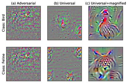
Figure 1: (Magnified) $\ell_{2}$ adversarial perturbations ($\epsilon=6.0$) towards two ImageNet-M10 classes, bird and feline: (a) standard adversarial perturbations towards two different classes generated on the same image, (b) universal adversarial perturbations, and (c) zooming in on the most semantic patch of (b).

We first observe that—in contrast to standard adversarial perturbations that tend to be incomprehensible—UAPs are more human-aligned (Figure 1). We dissect this phenomenon further by demonstrating that UAPs have two distinctive properties: (1) they are locally semantic, in that the signal is concentrated in local regions that are most salient to humans; and (2) they are approximately spatially invariant, in that they are still effective after translations. These properties make UAPs better aligned with human priors and distinguish them from standard perturbations.

Next, we study the extent to which UAPs leverage non-robust features [16], which are exploited by standard adversarial perturbations [16]. These are features that are sensitive to small perturbations, yet still correlated with the correct label [43]—in aggregate, their signal can be sufficient to generalize well on the underlying classification task.

As UAPs are better aligned with human priors, we might expect UAPs to contain signal that is more useful for generalization than standard adversarial perturbations. However, we find that this is not the case: UAPs contain significantly less generalizable signal from non-robust features compared to standard perturbations. We quantify this by following the methodology of Ilyas et al. [16] and measuring (1) how well a model can generalize to the original test set by training on a dataset where the only correlations with the label are added via UAPs; and (2) measuring the transferability of UAPs across independently trained models. Under these metrics, UAPs consistently obtain non-trivial but substantially worse generalization performance than standard adversarial perturbations.

2 Preliminaries

We consider a standard classification task: given input-label samples $(x,y)\in\mathcal{X}\times\mathcal{Y}$ from a data distribution $\mathcal{D}$, the goal is to learn a classifier $C:\mathcal{X}\rightarrow\mathcal{Y}$ that generalizes to new data.

2.1 Definitions

We focus on targeted perturbations generated by projected gradient descent (PGD).

Universal Adversarial Perturbations.

A universal adversarial perturbation [24], or UAP, is a perturbation $\delta\in\Delta$ that causes the classifier $C$ to predict the wrong label on a large fraction of inputs from $\mathcal{D}$, where $\Delta$ is the set of allowed perturbations. In contrast, a standard adversarial perturbation causes $C$ to predict the wrong label on one specific input. The only technical difference between UAPs and standard adversarial perturbations is the use of a single perturbation vector $\delta$ that is applied to all inputs. Thus, one can think of universality as a constraint for the perturbation $\delta$ to be input-independent.

Targeted perturbations.

We focus on targeted UAPs that fool $C$ into predicting a specific (usually incorrect) target label $t$. Thus, a (targeted) UAP $\delta\in\Delta$ satisfies $\mathbb{P}_{(x,y)\sim\mathcal{D}}[C(x+\delta)=t]=\rho$, where $\rho$ is the attack success rate (ASR) of the UAP. Targeted UAPs are the natural choice for our study here, as they allow us to isolate features (positively) correlated with a particular target. For a fair comparison, we also only consider targeted versions of standard adversarial perturbations. While we do not study untargeted UAPs, they generally perturb most examples towards a single common target [24]; this suggests that untargeted UAPs may have similar properties to the targeted versions.

$\ell_{p}$ perturbations.

We study the case where $\Delta$ is the set of $\ell_{p}$-bounded perturbations, i.e.

$$\Delta=\{\delta\in\mathbb{R}^{d}\>|\>||\delta||_{p}\leq\varepsilon\}$$

for $p=2,\infty$ where $\varepsilon>0$. This is the most widely studied setting for research on adversarial examples and has proven to be an effective benchmark [4]. Additionally, $\ell_{p}$-robustness appears to be aligned to a certain degree with the human visual system [43].

Projected gradient descent.

We focus on the family of perturbations computed by projected gradient descent (PGD), a standard method for generating adversarial examples. While there exists other methods for computing UAPs, which may have different properties, focusing on this family allows us to isolate universality as the sole factor of variation. From here on, we refer to our specific class of targeted, PGD-generated UAPs simply as UAPs.

2.2 Computing UAPs

We compute UAPs by using mini-batch projected gradient descent (PGD) to solve the following optimization problem:

$$\min_{\delta\in\Delta}\mathbb{E}_{(x,y)\sim\mathcal{D}}\Big{[}\mathcal{L}(f(x+\delta),t)\Big{]}$$ (1)

where $\mathcal{L}$ is the standard cross-entropy loss for classification, $f$ is the logits prior to classification, and $t$ is the target label. While many different algorithms have been developed for computing UAPs with varying ASRs, we use this simple algorithm instead as achieving the highest ASR is orthogonal to our investigations. As observed in Moosavi-Dezfooli et al. [24], UAPs trained on only a fraction of the dataset still generalize to the rest of the dataset, so in practice it suffices to approximate the expectation in (1) using a relatively small batch of samples drawn from $\mathcal{D}$. We call the batch we optimize over the base set, and use $K$ to refer to its size. We carefully choose hyperparameters (Section A.2) to ensure that our results remain robust.

2.3 Experimental Setup

Datasets.

We conduct our experiments on a subset of ImageNet [6] and CIFAR-10 [19]. The ImageNet Mixed10 dataset [7], which we refer to as ImageNet-M10, is formed by sub-selecting and grouping together semantically similar classes from ImageNet; it provides a more computationally efficient alternative to the full dataset, while retaining some of ImageNet’s complexity (see Section A.1 for more details). In the main text, we focus on ImageNet-M10, and in Appendix E we provide selected results on CIFAR-10 and full ImageNet.

Models.

We mainly focus on the standard ResNet-18 architecture [13], and highlight results obtained with other architectures in Section E.2.

3 Quantifying Human-Alignment

Standard $\ell_{p}$ adversarial perturbations are often thought to be incomprehensible to humans [42, 16]. Even when magnified for visualization, these perturbations are not identifiable to a human as belonging to their target class. In contrast, UAPs are visually much more interpretable: when amplified, they contain local regions that we can identify with the target class (see Figure 2 for example UAPs, and Figure 1 for a comparison to standard perturbations). Prior works have similarly observed that UAPs resemble their target class [12] or segmentation [14] and contain meaningful texture patterns [18, 21]

We quantify the extent to which UAPs are human-aligned beyond their visualizations. We identify two additional properties of UAPs—(1) semantic locality and (2) spatial invariance—which are well-aligned with human vision priors.

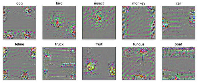
Figure 2: A sample of $\ell_{2}$ UAPs ($\epsilon=6.0$) for all ten ImageNet-M10 classes. We observe patterns resembling dog and cat (feline) heads, birds, outlines of cars and trucks, an insect, and mushrooms (fungus).

3.1 Semantic locality

We first find that UAPs locally semantic, in that a significant fraction of the signal in the perturbation is concentrated in small, localized regions that are salient to humans. This makes the perturbations more interpretable since the human visual system is known to attend to localized regions of images [33]; indeed, this property also motivates some attribution methods in interpretability [29]. Hence, we aim to quantify the extent to which UAPs possess this property.

While this property might seem to follow from the earlier observation that UAPs contain local regions that are semantically identifiable as the target class and standard perturbations do not (cf. Figure 2), this is not so obvious; a priori, it is unclear which parts of the perturbation influence the model. Here, we find that the UAPs are indeed locally semantic, in that most of their signal comes from the most visually meaningful regions. In contrast, standard perturbations lack this property as no local regions are semantic (as far as our current understanding of them).

Our methodology.

To quantify this for UAPs, we randomly select local patches of the perturbation, evaluate their attack success rate (ASR) in isolation, and inspect them visually. For both $\ell_{2}$ and $\ell_{\infty}$ perturbations, the patches with the highest ASR are more visually identifiable as the target class (Figure 3). This shows that the model is indeed influenced primarily by the most salient parts of the perturbation.

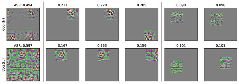
Figure 3: A randomized, local analysis of UAPs on ImageNet-M10. 64 random 80$\times$80 patches are isolated and evaluated on their ASR. First column shows the original perturbation for the target class (top: $\ell_{2}$; bottom: $\ell_{\infty}$); next five columns show three patches with the highest ASR, and two with the lowest. The number on top of each perturbation indicates its ASR on the test set. Patches are normalized to have the same norm as the highest norm patch.

3.2 Spatial invariance

We find that UAPs have the property of being spatially invariant to a large degree. As spatial invariance is one of the key properties of the human visual system [15], it is also a desirable, human-aligned property. In contrast, we demonstrate that standard adversarial perturbations are much more brittle to translations. Hence, this illustrates another way that UAPs are more human-aligned than standard perturbations.

Our methodology.

We quantify spatial invariance by measuring the ASR of translated perturbations. A highly spatially invariant perturbation will have a high ASR even after translations. Specifically, we compute targeted standard adversarial perturbations on a sample of 256 images from the ImageNet-M10 test set. Then, we evaluate the ASR of different translated copies of these perturbations over the respective images (e.g. translated copies of each perturbation are evaluated only on its corresponding image). For comparison, we take a precomputed set of UAPs of the same norm, and evaluate them across all 256 images. Translated perturbations use wrap-around to preserve information.

Figure 4 shows that UAPs still achieve non-trivial ASR after translations of varying magnitudes. In contrast, standard adversarial perturbations achieve a chance-level $10\%$ ASR when shifted by more than eight pixels (two grid cells in Figure 4). This illustrates that UAPs are somewhat robust to translations, and thus are more spatially invariant when compared to standard adversarial perturbations. In Appendix B, we discuss why we might expect to see such an invariance for UAPs.

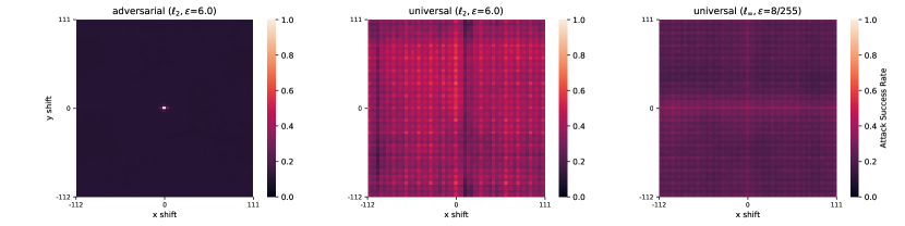
Figure 4: Evaluation of translated adversarial and universal $\ell_{2},\ell_{\infty}$ perturbations for the ImageNet-M10 class bird. We evaluate a subsampled grid with strides of four pixels. The value at coordinate $(i,j)$ represents the average ASR when the perturbations are shifted right by $i$ pixels and up by $j$, with wrap-around to preserve information; the center pixel at $(0,0)$ represents the ASR of the original unshifted perturbations. For UAPs, the ASR at each location is averaged over ten perturbations.

4 Quantifying Reliance on Non-Robust Features

So far, we have shown that UAPs possess desirable properties that standard adversarial perturbations lack, that make them more closely aligned with human priors. As human priors are believed to be important for generalization, we might expect that UAPs contain stronger signal for generalization than standard adversarial perturbations. Here, we find that despite their human-aligned properties, UAPs actually contain much less signal than standard adversarial perturbations.

We formalize this using the non-robust features model of Ilyas et al. [16]. We find that UAPs do indeed use non-robust features (that is, they modify useful correlations that models can rely on to generalize), but the non-robust features used by UAPs have significantly weaker signal than the non-robust features in standard adversarial perturbations.

4.1 The non-robust features framework

We first review the model proposed in Ilyas et al. [16]:

• A useful feature for classification is a function that is (positively) correlated with the correct label in expectation. Intuitively, a feature can be thought of as computing some property of the input, such as its color.

• A feature is robustly useful if, even under adversarial perturbations (within a specified set of valid perturbations $\Delta$), the feature is still useful.

• A useful, non-robust feature is a feature that is useful but not robustly useful. These features are useful for classification in the standard setting, but can hurt accuracy in the adversarial setting (since their correlation with the label can be reversed). For conciseness, throughout this paper we refer to such features simply as non-robust features.

Finally, we refer to the non-robust features leveraged by standard adversarial perturbations and UAPs as general non-robust features and universal non-robust features, respectively.

4.2 Two non-robust datasets: $\widehat{\mathcal{D}}_{adv}$ and $\widehat{\mathcal{D}}_{univ}$

Ilyas et al. [16] show that standard adversarial perturbations leverage non-robust features, and these features alone contain enough signal for generalization. They demonstrate this by constructing a dataset where the only features correlated with the label are those introduced by adversarial perturbations. Specifically, they construct a dataset $\widehat{\mathcal{D}}_{adv}$ (which they call $\widehat{\mathcal{D}}_{rand}$) which is modified from the original dataset as follows:

1. For each input-label pair $(x,y)$, select a target class $t$ uniformly at random; then

2. Compute an $\ell_{2}$ adversarial perturbation $\delta$ on $x$ targeted towards class $t$, and replace the original input-label pair $(x,y)$ with $(x+\delta,t)$.

By construction, $x$ and $t$ are un-correlated and the only features correlated with $t$ are those leveraged by $\delta$. And because $\delta$ is constrained to be within an $\ell_{2}$ ball, it can only yield non-robust features by def inition. Ilyas et al. [16] then train a network on $\widehat{\mathcal{D}}_{adv}$, and then evaluate its accuracy on a standard test set. The surprising finding is that—despite the fact that none of the examples in $\widehat{\mathcal{D}}_{adv}$ are correctly labeled from our perspective—the resulting classifier achieves non-trivial classification accuracy on the test set. Since the only signal comes from the non-robust features leveraged by the adversarial perturbations, this allows Ilyas et al. [16] to conclude that the adversarial perturbations must contain a non-trivial amount of signal useful for generalization.

Generalization from universal non-robust features.

To measure the amount of signal contained in UAPs, we perform the same experiment as above, except we replace the standard adversarial perturbations in Step 2 with UAPs. We call the resulting dataset $\widehat{\mathcal{D}}_{univ}$. We visualize this process in Figure 5. The only difference from the previous setup is that the features that remain correlated with $t$ are those leveraged by UAPs. As long as the test accuracy on the (unaltered) test set of a model trained on $\widehat{\mathcal{D}}_{univ}$ is non-trivial, we can conclude (similarly to Ilyas et al. [16]) that UAPs are leveraging non-robust features. By comparing the resulting test accuracy to that achieved on $\widehat{\mathcal{D}}_{adv}$, we can gauge the relative strength of generalizable signal contained in UAPs compared to standard perturbations.

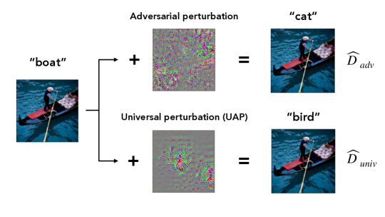
Figure 5: Construction of $\widehat{\mathcal{D}}_{adv}$ and $\widehat{\mathcal{D}}_{univ}$ datasets. The perturbed image is labeled with the target of the respective perturbation.

Replicating the original setup of $\widehat{\mathcal{D}}_{adv}$ for $\widehat{\mathcal{D}}_{univ}$ requires a few additional considerations. In Section C.1, we discuss them in detail.

Results.

We train new ResNet-18 models on the $\widehat{\mathcal{D}}_{adv}$ and $\widehat{\mathcal{D}}_{univ}$ datasets and evaluate them on the original test set. The best generalization accuracies from training on $\widehat{\mathcal{D}}_{univ}$ and $\widehat{\mathcal{D}}_{adv}$ were 23.2% and 74.5%, respectively. This indicates that universal non-robust features do have signal that models can use to generalize, but universal non-robust features are harder to generalize from than general non-robust features. Thus, there is some useful signal in universal non-robust features, but there appears to be less of it than in standard adversarial perturbations.

4.3 Transferability of UAPs

Another way to quantify the extent to which UAPs leverage non-robust features is by studying their transferability. Ilyas et al. [16] suggest that the pervasive transferability of adversarial perturbations [30, 24] can be attributed to different models relying on common non-robust features. Consequently, perturbations that leverage more shared non-robust features should transfer better across models. Here, we are primarily interested in transferability as a proxy for detecting shared non-robust features, and we compare the transferability of standard and UAPs.

Figure 6: Comparing transferability of standard adversarial and universal adversarial $\ell_{2}$ perturbations ($\epsilon=6.0$): perturbations are generated on the source model (ResNet-18), then transferred to a different target model: (left) another ResNet-18 model trained from a different random initialization, and (right) a VGG16 model. Standard adversarial perturbations have a higher transfer success rate across all classes.

To measure transferability, we (1) perturb examples using either a standard adversarial perturbation or a UAP on the source model, and (2) measure the probability that the perturbed input is classified as the target class on a new target model (an independently trained ResNet-18 and VGG16 model). For normalization, to make standard and UAPs comparable, we only consider perturbed images that are misclassified by the source model, and also evaluate transfer on images that have labels different from the target label. Figure 6 shows that UAPs transfer much less effectively to both target models, suggesting that universal non-robust features are shared across models to a smaller extent than general non-robust features. In Appendix C, we provide additional analyses for results in this section.

4.4 Interpolating Universality

The above experiments demonstrate that while UAPs are more human-aligned, they leverage only a small fraction of the statistical signal in general non-robust features. To explore the underlying trade-off, we investigate to what extent one can interpolate between the properties of universal and standard non-robust features. We explore two different methods of “interpolating” universality: varying the number of images (Section 4.4) and varying the diversity of images (Section 4.4).

UAPs over smaller base sets.

One natural way to interpolate universality is to vary $K$, the size of the base set (cf. Section 2.2). $K=1$ corresponds to standard adversarial perturbations, and large enough $K$ corresponds to fully universal perturbations. We generate UAPs over different choices of $K$, and repeat the experiment from Section 4.2. Table 2 shows that signal for generalization generally decreases with the size of the base set. Notably, generalization begins to suffer even for relatively small values of $K$. For example, the generalization accuracy falls from $74\%$ at $K=1$ to just $34\%$ at $K=16$.

Table 1: Interpolating universality: generalization from $\widehat{\mathcal{D}}_{univ}$ constructed using UAPs generated with smaller base sets.

Size of base set ($K$)	Test Accuracy (%)
1	74.5
2	57.1
4	61.3
8	57.4
16	34.3
32	21.8
256	19.1

Table 2: Generalization from class-universal and sub-class universal non-robust features.

Source Class	Test Accuracy (%)
Random	23.2
Single Class	23.9
Single Sub-class	27.1

In contrast, Figure 7 shows that the semantic quality of UAPs improves as the base set becomes larger. This suggests a possible trade-off between how human-aligned perturbations are and the amount of statistical signal, at least when interpolating along this particular axis. However, the exact nature of this trade-off is not obvious: better semantics only become obvious at higher values of $K$ ($\gtrsim 64$), whereas generalization suffers even at relatively small values of $K$ ($\sim 16$). Additional analysis in Section C.4 suggests that optimizing over multiple images has a non-linear effect, even at small values such as $K=2$.

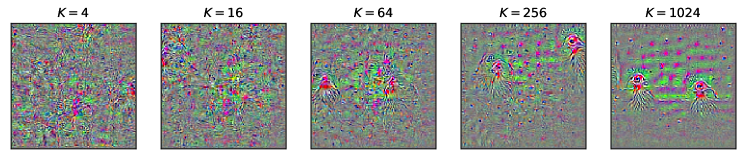
Figure 7: Visualization of UAPs for target bird, computed over base sets of different size $K$. We observe that the visual quality improves with the size of the base set.

UAPs over images of restricted diversity.

We next look at the influence of a different factor in our observed phenomena: the semantic diversity of images in the base set. In particular, consider class universal and subclass universal perturbations, where we restrict the base set to examples from a single class (e.g., dog) or subclass (one original ImageNet class, e.g., Terrier). We repeat the experiments from Section 4.2 using these perturbations (cf. Table 2); the generalization on the original test set improves only modestly.

The results of these interpolation experiments show that the large gap in signal between UAPs and standard perturbations persists even when the level of “universality” is relaxed.

5 Related Work

In this section, we discuss connections to prior related work.

Universal adversarial perturbations.

Moosavi-Dezfooli et al. [24] first introduce UAPs for classification models. Many follow-up works explore different methods to generate them, using data-independent algorithms [26, 21], singular vectors of model Jacobians [18], generative models [31, 12], and other techniques [44]. A priori, it is not obvious why UAPs are so prevalent; Moosavi-Dezfooli et al. [25] shows via theory and experiments that the prevalence of UAPs is related to the curvature of the decision boundary. Beyond image classification, other works [14, 27] study UAPs for semantic image segmentation. Hendrik Metzen et al. [14] find that UAPs generated for a fixed target segmentation exhibit local structures that resemble the target scene, analagous to the observations made here.

Robustness and UAPs.

While the majority of research on adversarial robustness focuses on standard perturbations, prior works also study the robustness of models to UAPs. Models trained via standard adversarial training [22] are known to be more robust to UAPs than standard models [27]. Mummadi et al. [27] explore this further and uses shared adversarial training, which computes UAPs on the mini-batch and uses them for adversarial training. Further, they study UAPs computed on these robustly trained models, and find that they are much more perceptible than UAPs computed on standard models. Shafahi et al. [38] take a different approach to training, maintaining a global UAP and optimizing it in parallel with model parameters via alternating SGD.

UAPs and features.

A few prior works also study UAPs from the perspective of understanding their features. Using ideas from analysis of universal perturbations, Jetley et al. [17] find that class-specific patterns unintelligible to humans can induce misclassification while also being essential for classification. Zhang et al. [46] also study the UAPs and their features by analyzing correlations in the representation space. Their analysis contrasting UAPs and standard adversarial perturbations is complementary to ours; for instance, our results on spatial invariance is consistent with their finding that UAPs behave as the “dominant” feature when added to images.

Non-robust features.

Tsipras et al. [43] first formalize non-robust features via a simple theoretical model and study the tradeoffs between robustness and accuracy. Ilyas et al. [16] develop these ideas further and demonstrate that non-robust features alone are sufficient for generalization on standard image classification datasets. In particular, their analysis shows that adversarial examples are a consequence of misalignment between non-robust features and human priors. Conversely, several works discuss the usefulness and perceptual alignment of robust features [43, 36], which can be extracted from adversarially robust models.

Feature visualizations.

Many works propose saliency map methods to construct visualizations of features learned by networks [40, 34, 41, 5]. While many of these maps are visually appealing, they often rely on post-processing, and their visual appeal can be misleading [1]. In contrast, our visualizations of UAPs involve no post-processing, yet show a striking difference between universal and standard adversarial perturbations.

6 Conclusion

In this work, we revisit (targeted) universal perturbations and show that they exhibit human-aligned properties that distinguish them from standard adversarial perturbations. In particular, we precisely characterize the degree to which they are human-aligned in terms of two properties: semantic locality and spatial invariance. We further quantify the degree to which UAPs leverage non-robust features through experiments on their generalizability and transferability, and find that UAPs contain much weaker signal than standard perturbations. Our study demonstrates that examining UAPs may be a fruitful direction for understanding more fine-grained properties of adversarial perturbations, and associated phenomena such as the prevalence and the nature of non-robust features.

Appendices

Appendix A describes the experimental setup and selection of all hyperparameters. Appendices B, C, D, E, F, G and H give more detailed analyses and additional results: Appendix B discusses intuition for the translational invariance observed in Section 3.2. Appendix C provides more results and analyses for generalization experiments in Section 4. Appendix D provides an alternate scaling analysis to differentiate robust and non-robust signals. Appendices E, F and G gives a selection of additional results for experiments for Section 3 across different settings. Appendix H discusses the diversity of universal perturbations.

Appendix A Experimental Setup

A.1 Datasets

Our experiments use CIFAR-10 and ImageNet-M10, a subset of ImageNet ILSVRC2012 [35]; we focus primarily on ImageNet-M10.

ImageNet-M10 consists of ten super-classes, each corresponding a WordNet [23] ID in the hierarchy. Different super-classes contain varying number of ImageNet classes, so the dataset is balanced by choosing six classes within each super-class. The class numbers of the corresponding ImageNet classes are shown in Table 3. The super-classes correspond to the ten labels for the classification task; for experiments using fine-grained labels, we use the 60 ImageNet classes as labels. A sample image from each class is shown in Figure 8.

Table 3: ImageNet classes used in the ImageNet-M10 dataset.

Class	WordNet ID	Corresponding ImageNet Classes
“Dog”	n02084071	151 to 156
“Bird”	n01503061	7 to 12
“Insect”	n02159955	300 to 305
“Monkey”	n02484322	370 to 375
“Car”	n02958343	407, 436, 468, 511, 609, 627
“Feline”	n02120997	286 to 291
“Truck”	n04490091	555, 569, 675, 717, 734, 864
“Fruit”	n13134947	948, 984, 987 to 990
“Fungus”	n12992868	991 to 996
“Boat”	n02858304	472, 554, 576, 625, 814, 914

The ImageNet-M10 dataset can be used easily on top of a standard ImageNet directory by loading the mixed_10 dataset from the robustness library [7].

ImageNet-M10 is comparable in size and complexity to restricted ImageNet, which has been used for adversarial robustness research [16, 36].

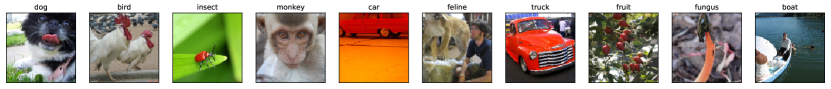
Figure 8: Sample images from each (super) class of ImageNet-M10.

A.2 Hyperparameters

All experiments in the paper involve a combination of: training models, computing standard adversarial perturbations, and computing UAPs. Below, we provide details for all the hyperparameters and their selection.

Robustness threshold We use the same robustness threshold throughout: $\ell_{2},\epsilon=6.0$ and $\ell_{\infty},\epsilon=8/255$ for ImageNet datasets, and $\ell_{2},\epsilon=1.0$ for CIFAR-10.

A.2.1 Training models

Training base models All models are trained with SGD with momentum and standard data augmentation. For corresponding robust models, the same optimization parameters are used with projected gradient descent (PGD) [22] using 3 steps and attack step size $\frac{2}{3}\epsilon$ (for both $\ell_{2}$ and $\ell_{\infty}$). Weight decay of $5\cdot{10}^{-4}$ was used in all cases. The accuracies of these models are shown in Table 4.

Table 4: Standard and robust models (ResNet-18) used in our experiments.

Dataset	Model	Standard Test Accuracy (%)	Robust Test Accuracy (%)
ImageNet-M10	Standard	95.7	$<1.0$
	$\ell_{2}$	86.7	59.8
	$\ell_{\infty}$	87.6	59.2
CIFAR-10	Standard	94.8	$<1.0$
	$\ell_{2}$	80.0	50.7

Training models on constructed datasets The models are trained on the constructed datasets, including $\widehat{\mathcal{D}}_{univ}$ and $\widehat{\mathcal{D}}_{adv}$ (Section 4.2), over the following grid of hyperparameters: three learning rates (0.01, 0.05, 0.1), two batch sizes (128, 256), including/ not including a single learning rate drop by a factor of 10. All models are trained with 400 epochs, standard data augmentation, and weight decay $5\cdot 10^{-4}$. We report the setting corresponding to the highest test accuracies in Table 5.

As an exception, for the $K$-interpolated datasets (Section 4.4), we fixed a single set of hyperparameters to train the models.

Table 5: Default and best hyperparameters for training models on different datasets.

Source Dataset	Constructed Dataset	Epochs	LR	Batch Size	LR Drop
ImageNet-M10	$\mathcal{D}$ (original)	200	0.1	256	50, 100, 150
	$\widehat{\mathcal{D}}_{adv}$ ($\ell_{2}$)	400	0.01	128	250
	$\widehat{\mathcal{D}}_{univ}$ ($\ell_{2}$, random class)	400	0.01	128	250
	$\widehat{\mathcal{D}}_{univ}$ ($\ell_{2}$, $K$-interp)	400	0.01	256	250
	$\widehat{\mathcal{D}}_{univ}$ ($\ell_{2}$, same class)	400	0.05	64	None
	$\widehat{\mathcal{D}}_{univ}$ ($\ell_{2}$, same subclass)	400	0.05	128	250
	$\widehat{\mathcal{D}}_{adv}$ ($\ell_{\infty}$)	400	0.001	256	None
	$\widehat{\mathcal{D}}_{univ}$ ($\ell_{\infty}$)	400	0.1	128	None
CIFAR-10	$\mathcal{D}$ (original)	150	0.1	128	50, 100
	$\widehat{\mathcal{D}}_{adv}$ ($\ell_{2}$)	400	0.05	256	250
	$\widehat{\mathcal{D}}_{univ}$ ($\ell_{2}$)	400	0.05	256	None

A.2.2 Computing adversarial perturbations

Adversarial perturbations For a given $\epsilon$, PGD with an attack step size of $\frac{\epsilon}{3}$ and 10 steps is used (no random restarts.)

Universal perturbations The hyperparameters of the PGD algorithm for universal perturbations (Section 2.2) are: learning rate schedule, number of epochs, and batch size. In order to see the impact of the choice of these parameters, we ran a grid search over the parameters; a sample of these selections is visible in Figure 9. Overall, we observe that the exact choice of these parameters did not have a large impact on the final training accuracy (and the quality of the resulting perturbations, both in terms of visuals and generalization to other images) as long as (1) the initial learning rate is not too low or too high, and (2) a sufficient number of epochs is used. So in all of our experiments, we fix a learning rate of 2.0 and a batch size of 128 or 256, and trained a sufficient number of epochs (max of 100). The use of a learning rate decay did not seem to have much impact, so we use the same learning rate throughout.

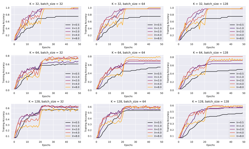
Figure 9: The learning dynamics of computing universal perturbation (epoch vs. training accuracy on the base set) are shown across a selection of learning rates, batch sizes, and three intermediate values of $K$.

A.3 Computing resources

Experiments were run primarily on 8 NVIDIA GeForce GTX 1080 Ti GPUs.

Appendix B Invariance of UAPs

Intuitively, it may not be surprising that UAPs are translationally invariant, given the input-independence of UAPs. We sketch an argument that formalizes this intuition.

First, by definition, a universal perturbation is (with high probability) effective against both image $x$, and its translation $T(x)$, where $T$ is a translation operation from the group of translations (with wrap-around), as we expect $T(x)$ as a sample from the same underlying distribution. Now, consider the image $T(x)+\delta$ where $\delta$ is a universal perturbation. If we assume that our models are reasonably translationally invariant, it will classify $T(x)+\delta$ similarly as $T^{-1}(T(x)+\delta)=x+T(\delta)$, where $T^{-1}$ is the inverse translation. Hence, $T(\delta)$ should also be an effective perturbation for $x$. Since $x$ was arbitrary, $T(\delta)$ is a universal perturbation.

More generally, we expect UAPs to be invariant to transformations under which our input distribution is also invariant to.

Appendix C Additional Analyses for Section 4

C.1 Design considerations

Replicating the original setup of $\widehat{\mathcal{D}}_{adv}$ for $\widehat{\mathcal{D}}_{univ}$ requires a few additional considerations, due to the different nature of UAPs.

Diversity of perturbations. Firstly, it is rather expensive to compute a separate UAP for each input, so we compute and use the same UAP per batch of inputs. One possible concern is that re-using same perturbations across the batch results in a reduction in “diversity” of features considered. We ran additional experiments to control for this, but found that increasing the number of unique UAPs used only marginally increases the generalization, and does not impact any of the global trends. Further, increasing the visual diversity of perturbations via other methods also had limited impact on increasing generalization (see Appendix H for methods to increase diversity).

UAPs fail on some inputs. Another complication is that for the robustness threshold $\epsilon$ considered here, universal perturbations fool models only on a fraction $\rho$ of all training examples (while adversarial perturbations at the same threshold succeed on all examples). Hence, we only include examples on which the UAP succeeds (i.e., a pre-trained model classifies the perturbed input as $t$). This filtering step reduces the size of the dataset, so we decrease the number of examples in $\widehat{\mathcal{D}}_{adv}$ accordingly in our evaluation. We also ensure that the distribution of new and original labels is uniform and independent so that the original label is uncorrelated with the new label.

C.2 All results on generalization on non-robust datasets

Here we collect additional results for the generalization experiment across various settings: $\ell_{2},\ell_{\infty}$ perturbations in ImageNet-M10 and $\ell_{2}$ perturbations on on CIFAR-10. We did not conduct experiments on ImageNet, as the constructions of the datasets is computationally too intensive.

Table 6 shows that there is consistently much lower generalization from $\widehat{\mathcal{D}}_{univ}$ than from $\widehat{\mathcal{D}}_{adv}$.

Table 6: Generalization from constructed datasets.

Source Dataset	Perturbation Set	Constructed Dataset	Test Accuracy (%)
ImageNet-M10	$\ell_{2},\varepsilon=6.0$	$\widehat{\mathcal{D}}_{adv}$	74.5
ImageNet-M10	$\ell_{2},\varepsilon=3.0$	$\widehat{\mathcal{D}}_{adv}$	76.6
ImageNet-M10	$\ell_{2},\varepsilon=6.0$	$\widehat{\mathcal{D}}_{univ}$	23.2
ImageNet-M10	$\ell_{\infty},\varepsilon=8/255$	$\widehat{\mathcal{D}}_{adv}$	78.7
ImageNet-M10	$\ell_{\infty},\varepsilon=8/255$	$\widehat{\mathcal{D}}_{univ}$	26.5
CIFAR-10	$\ell_{2},\varepsilon=1.0$	$\widehat{\mathcal{D}}_{adv}$	64.3
CIFAR-10	$\ell_{2},\varepsilon=1.0$	$\widehat{\mathcal{D}}_{univ}$	23.3

C.3 Bounding robust feature leakage

The accuracies on the $\widehat{\mathcal{D}}_{univ}$ datasets are very low (for comparison, they are even lower compared to a ResNet-18 model trained on (fixed) randomly initialized features, which achieve an accuracy greater than 30%). Given this, one concern is that the small signal we observe can be entirely accounted for by leakage of robust features into these datasets [16, 9]: while a small perturbation cannot entirely flip the correlation of a robust feature, it can still induce a small correlation on average on the $\widehat{\mathcal{D}}_{univ}$ dataset. Even if there are no non-robust features that are perturbed, the small “leaked” correlations from the robust features alone could allow for generalization from $\widehat{\mathcal{D}}_{univ}$ to the original test set.

We run several additional experiments to bound the amount of leakage (we focus on $\ell_{\infty}$ perturbations on ImageNet-M10):

• We construct a dataset similar to $\widehat{\mathcal{D}}_{det}$ [16] but instead using universal perturbations, where we choose new corrupted labels by cyclically shifting original labels, rather than choosing them randomly; the robust features now point away from the label. Models trained on this new dataset achieve an accuracy up to 19.1% on the original test set, which is less than 26.5% from $\widehat{\mathcal{D}}_{univ}$, but still well above chance-level of 10%. This demonstrates that there is residual signal in universal perturbations that cannot be entirely accounted for by robust leakage.

• We can also probe the original dataset by seeing how well different features can fit the dataset. Adapting the procedure in Goh [9], we take pre-trained features from different natural and $\ell_{\infty}$ robust models on ImageNet-M10, and train a linear classifier over those features on $\widehat{\mathcal{D}}_{univ}$. The results in Table 7 show that features from natural models, even sourced from a different model than the one used to generate $\widehat{\mathcal{D}}_{univ}$ or from a different architecture, capture more of the signal in $\widehat{\mathcal{D}}_{univ}$ than robust features. For comparison, the model trained on $\widehat{\mathcal{D}}_{univ}$ from scratch, as we saw earlier, achieves an accuracy of 26.5%, which is higher than 22.3%. This demonstrates again that while some leakage is happening, it cannot account for all of the signal in universal perturbations.

  Table 7: Training on $\widehat{\mathcal{D}}_{univ}$ using fixed features to check for leakage. The gap between the last row (robust) and others suggest that there are indeed non-robust features being utilized beyond (leaked) robust features.

  Feature Source	(Fine-tuned) Test Accuracy (%)
  natural	36.9
  natural, diff init	35.0
  natural, diff arch (VGG16)	26.4
  robust ($\ell_{\infty}$)	22.3

These results consistently show that while some robust leakage occurs, it cannot account for all of the signal in universal perturbations. A small but non-trivial amount of signal comes from the universal non-robust features.

C.4 Evidence of interaction between images in the base set

The degradation in the non-robust signal at even small values of $K$ is striking. One plausible hypothesis for the degradation of signal quality between $K=1$ and $K>1$ is that optimizing the perturbation over more images splits the effective perturbation norm budget, and is akin to optimizing over each image separately with a reduced budget, say $\epsilon/K$. To test this hypothesis, we constructed standard adversarial perturbations with a reduced budget of $\epsilon=3.0$. This corresponds to the setting $K=1,\epsilon=3.0$. We compare the generalization from this new dataset to that from the $K=2,\epsilon=6.0$ case in Table 8 (latter is the same value as in Table 2), which should be similarly effective if the norm budget hypothesis is correct. We instead find that the standard adversarial perturbation at a smaller norm of $\epsilon=3.0$ results in much hire generalization accuracy. Given the large gap, it seems unlikely that this simple norm budget sharing can explain the above interpolation phenomena. This suggests that when universal perturbations are computed jointly over multiple images, the perturbations are of a fundamentally different nature. This may be due to the perturbation having to interact with different non-robust features present in different images.

Table 8: Comparing generalization from two different constructed datasets for ImageNet-M10 using $\ell_{2}$ perturbations. $K$ is the base set size; $K=1$ corresponds to using standard adversarial perturbations, and $K=2$ to computing perturbations over random pairs of images.

Perturbation Type	Test Accuracy on Original (%)
$\epsilon=6.0$, $K=2$	57.1
$\epsilon=3.0$, $K=1$	76.6

C.5 Alternate base sets

In this paper, we focused on computing universal perturbations over base sets (cf. Section 2.2) consisting of different images (from possibly a restricted set of classes). To study the importance of sample diversity in the base set, we computed universal perturbations over the base set consisting of $K$ different augmentations of a single image. The resulting universal perturbations still have similar (but less salient) visual characteristics, and are transferable but to a lesser degree than perturbations computed over base set of different images.

Appendix D Scaling Analysis

Results of Section 4 and  Section C.3 show that universal perturbations are leveraging non-robust features. However, they do not entirely rule out contributions from robust features, and suggest some robust feature leakage may be occurring. If universal perturbations are also relying on robust features, we cannot necessarily attribute the semantic aspects of the perturbation that we observed earlier (and which we showed to be responsible for most the ASR) to non-robust features. Nonetheless, here we provide evidence that robust leakage is unlikely to be a primary contribution to the signal.

Scaling analysis on natural vs. robust model
Our analysis based on the following premise: if the universal perturbations are primarily relying on small perturbations of robust features, then a robust model should eventually react when we amplify the signal in the universal perturbations. We currently lack tools to selectively control robust and non-robust contents of an image within the $\ell_{p}$ ball, so we settle for a simpler proxy.

Below, we first show that simply linearly scaling the perturbation can effectively tune the strength of the signal. More precisely, given a universal perturbation $\delta$, we evaluate the ASR of $t\cdot\delta$, where $t$ is a scaling parameter. When we perform this scaling on a natural (non-robust) model, the ASR increases as we increase $t$ (Figure 10). (This holds even if networks used to train the universal perturbation and the one used to evaluate its ASR differ.) If there was significant robust leakage, we would expect a similar qualitative behavior for the robust model. Instead, we find that the robust model does not react to any scaling of the perturbation. On the other hand, a universal perturbation of norm $\epsilon=30.0$ is computed on an adversarially-trained robust model ($\epsilon=6.0$) still fools the natural model, even when scaled down. Together, these findings suggest that universal perturbations computed on the natural model are unlikely to leverage robust features used by the robust model.

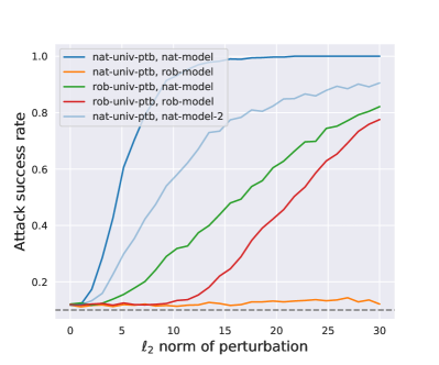
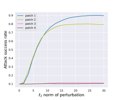
Figure 10: Scaling analysis of universal perturbations on ImageNet-M10: (Left) we generate a universal perturbation (nat-univ-ptb) of $\ell_{2}$ norm $\epsilon=6.0$ on a natural model (nat-model) for the target bird, and measure the sensitivity of the natural and a robust model (rob-model) at various rescalings of the perturbation. We also generate a universal perturbation (rob-univ-ptb) of norm $\epsilon=30.0$ for the robust model and use it to show that the robust model does react to scalings of some perturbation. The same nat-univ-ptb is also evaluated on an independent natural model (nat-model-2) for control; (Right) different cropped local patches of the same nat-univ-ptb are also evaluated on the natural model

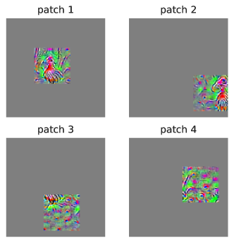
Figure 11: Visualizations of the cropped patches used in Figure 10 (Right)

In fact, a more fine-grained scaling analysis shows that the signal is indeed primarily amplified in the semantic parts of the image. In Section 3 we already observed that models are most sensitive to the most semantic parts of universal perturbations; here we check that the order remains consistent across various scales. We repeat the above scaling evaluation on natural vs. robust models, except we scale only patches of the perturbation, of varying levels of semantic content (Figure 10). As before, we find that none of the patches, even after scaling, trigger the robust network. On the non-robust models, the relative effectiveness of local patches is consistent with their semantic content: patches that are more semantically identifiable have more signal at all scales.

The above analysis shows that universal perturbations are likely primarily targeting non-robust features. Combined with our findings earlier in Section 3, this shows that non-robust features may not be entirely unintelligible to humans. Our visualizations (Figure 11) suggests that universal non-robust features may be capturing intuitive properties, such as the presence of a faint bird head. Thus, non-robustness in networks may partially arise from relying on cues that are small in magnitude but still human-aligned.

Appendix E Visualizations

We show visualizations of universal perturbations across different datasets (CIFAR-10, ImageNet-M, and ImageNet), architectures (VGG for Mixed10), and norm constraint ($\ell_{\infty}$ for Mixed10) to illustrate the generality of the phenomena observed.

Normalization for visualization.

For all visualizations, perturbations were rescaled as follows (for each input channel): first truncated to $[-3\sigma,3\sigma]$ (where $\sigma$ is the standard deviation across all channels and pixels), then rescaled and shifted to lie in $[0,1]$.

E.1 Different datasets

See Figures 12 and 13.

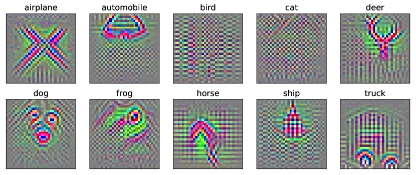
Figure 12: Visualization of $\ell_{2}$ universal perturbations at $\epsilon=1.0$ for a CIFAR-10 model. Optimization on some classes (bird and cat) fail occasionally, and is reflected in their lack of semantic content.

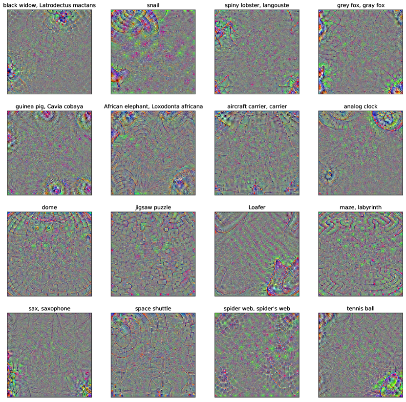
Figure 13: Visualization of $\ell_{2}$ universal perturbations at $\epsilon=6.0$ for a full ImageNet model. We hand-picked the classes with the most salient perturbations. Many of the perturbations possess visual characteristics identifiable with the corresponding class.

E.2 Other architectures

See Figure 14.

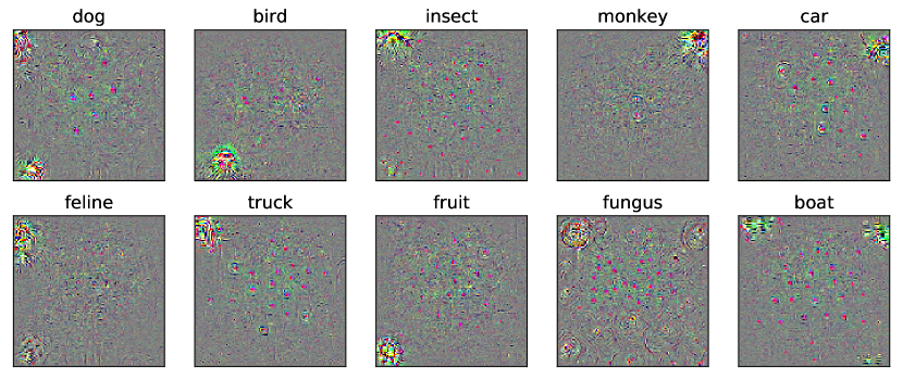
Figure 14: Visualization of $\ell_{2}$ universal ($K=512$) perturbations at $\epsilon=6.0$ for ImageNet-M10, generated this time on a VGG11 network [39].

E.3 $\ell_{\infty}$ perturbations

See Figure 15.

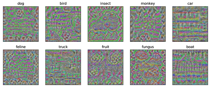
Figure 15: Visualization of $\ell_{\infty}$ universal perturbations at $\epsilon=8/255$ for different target classes. We observe recognizable patterns for each class similar to those of $\ell_{2}$ universal perturbations, but the remaining regions have much higher energy and different texture.

Appendix F Locality Analysis

We provide full results of randomized locality analysis on ImageNet-M10 in Figures 16 and 17. We did not perform the analysis on CIFAR-10 perturbations, as the perturbations are more “global” by nature, e.g. the semantic part seems to already occupy most of the perturbation.

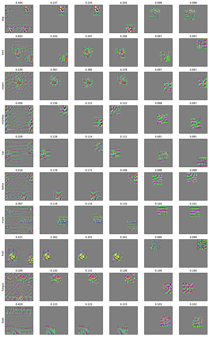
Figure 16: Locality analysis of $\ell_{2}$ universal perturbations on ImageNet-M10. Each row shows the perturbation for the particular class, followed by three patches with highest ASR and two patches with lowest ASR; ASR is written above each patch.

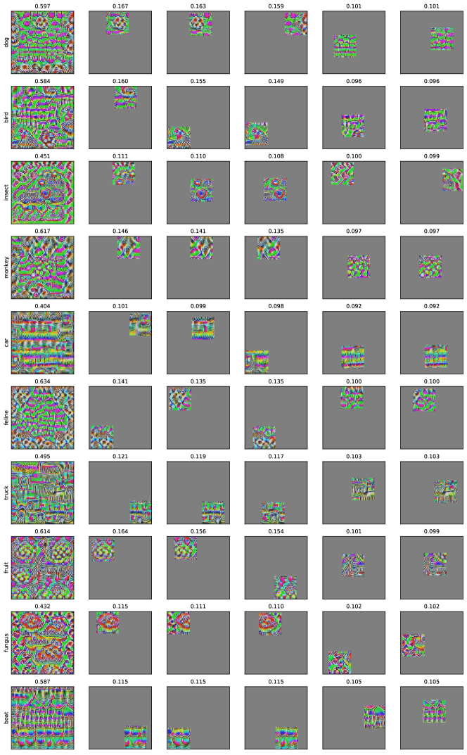
Figure 17: Locality analysis of $\ell_{\infty}$ universal perturbations on ImageNet-M10. Each row shows the perturbation for the particular class, followed by three patches with highest ASR and two patches with lowest ASR; ASR is written above each patch

Exploring properties of $\ell_{2}$ vs $\ell_{\infty}$ perturbations. For both $\ell_{2}$ and $\ell_{\infty}$ universal perturbations, the patches that are most identifiable with their classes have much higher ASR. A major difference is that for $\ell_{2}$ perturbations, the patches with low ASR have much smaller norms, whereas for $\ell_{\infty}$ perturbations, the patches with low ASR have the similar norms (measured in either $\ell_{2}$ or $\ell_{\infty}$). This is expected, as for $\ell_{2}$ every local patch contributes to the total $\ell_{2}$ norm and it is unsurprising that optimization avoid putting weight on patches with little signal; in contrast, for $\ell_{\infty}$ perturbations, different patches are independent in meeting the norm bound, so the perturbation can have patches with low signal that are similar in norm. However, it is not clear whether these low signal patches found by optimization serve some purpose. To test this, we experimented with zeroing-out these patches or replacing them with copies of patches with the highest ASR. Evaluation of the resulting perturbations show that the ASR is highest with these patches in place, and are in fact lowered when we replace them with patches with higher ASR. This suggests that these low signal patches have a non-linear interaction with rest of the perturbation, and are providing a small boost in signal when combined with other patches. Understanding this phenomena in more depth may shed more light on the differences between properties of $\ell_{\infty}$ and $\ell_{2}$ universal perturbations.

Appendix G Spatial Invariance

Section 3.2 shows a sample of translation invariance evaluation for perturbations on ImageNet-M10. We include additional samples from evaluation using $\ell_{2}$ perturbations on CIFAR-10, to check that the phenomena is general.

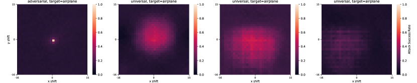
Figure 18: We evaluate attack success rates of translated adversarial and universal perturbations for different target classes over the test set on CIFAR-10. There is no subsampling of the grid here as the dimensions are much smaller. We used a subsampled grid of all the possible offsets with strides of four pixels. As before, the value at coordinate $(i,j)$ represents the average attack success rate when the perturbations are shifted by $i$ pixels along the $x$-axis and $j$ pixels along the $y$-axis, with wrap around to preserve information. Evaluation of adversarial perturbation is only shown for one target as it is redundant.

Appendix H Perturbation Diversity

Throughout our investigations, we observed that the computed universal perturbations seemed to lack in diversity. We see in Figure 19 (first row) that generating multiple different universal perturbations for a given target leads to visually similar perturbations. Prior works study generating more diverse universal perturbations [32].

To increase diversity, we generated universal perturbations with an additional penalty to encourage orthogonality of perturbed representations at different layers of the network. Even with the added regularization, the resulting perturbations appear to be remain similar, but with changes in spatial arrangements of the semantic patterns (second row).

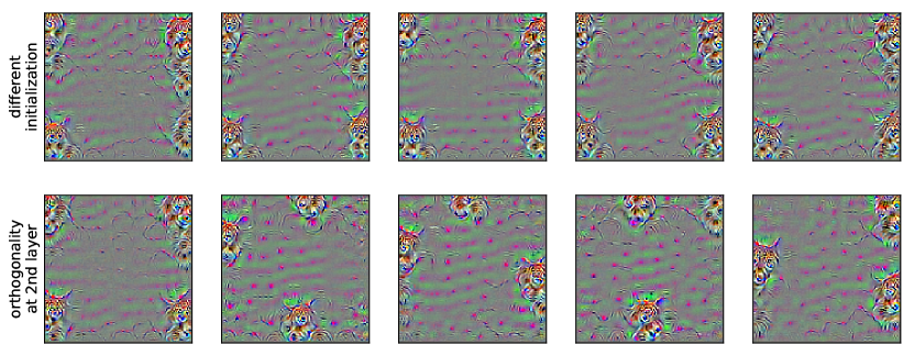
Figure 19: Visualization of $\ell_{2}$ universal perturbations for class feline, computed using different initializations (first row), and an additional penalty to encourage diversity (second row).

One effective way we found to increase the diversity of these perturbations is to compute universal perturbations for targeting specific sub-classes of Mixed10. To do so, we first train a fine-grained model using Mixed10’s subclass labels, and generate universal perturbations for each of the six sub-classes per class. In Figure 20, we show the universal perturbations targeting individual sub-classes of the bird class. We observe distinct patterns characteristic of each species of birds, an increase in diversity from before. However, generation of these perturbations requires a model trained on the fine-grained labels. An interesting question is whether one can recover such diversity using just the model trained on coarse-grained labels without injection of additional label information.

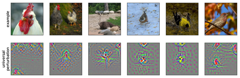
Figure 20: Visualization of $\ell_{2}$ universal perturbations for six individual sub-classes inside the bird class. These were generated on a fine-grained model trained on the subclass labels (60 in total). Observe the distinctive visual characteristics of each class, for instance the outline of a chicken (column 2), the neck of an ostrich (column 3), and the distinctive colors of different species (columns 3-5).

References

- Adebayo et al. [2018] Julius Adebayo, Justin Gilmer, Michael Muelly, Ian Goodfellow, Moritz Hardt, and Been Kim. Sanity checks for saliency maps. In Neural Information Processing Systems (NeurIPS), 2018.
- Benz et al. [2020] Philipp Benz, Chaoning Zhang, Tooba Imtiaz, and In So Kweon. Double targeted universal adversarial perturbations. In Proceedings of the Asian Conference on Computer Vision, 2020.
- Carlini and Wagner [2017] Nicholas Carlini and David Wagner. Towards evaluating the robustness of neural networks. In 2017 IEEE Symposium on Security and Privacy, 2017.
- Carlini et al. [2019] Nicholas Carlini, Anish Athalye, Nicolas Papernot, Wieland Brendel, Jonas Rauber, Dimitris Tsipras, Ian J. Goodfellow, Aleksander Madry, and Alexey Kurakin. On evaluating adversarial robustness. In ArXiv preprint arXiv:1902.06705, 2019.
- Carter et al. [2019] Shan Carter, Zan Armstrong, Ludwig Schubert, Ian Johnson, and Chris Olah. Activation atlas. Distill, 2019. doi: 10.23915/distill.00015. https://distill.pub/2019/activation-atlas.
- Deng et al. [2009] J. Deng, W. Dong, R. Socher, L.-J. Li, K. Li, and L. Fei-Fei. ImageNet: A Large-Scale Hierarchical Image Database. In CVPR09, 2009.
- Engstrom et al. [2019] Logan Engstrom, Andrew Ilyas, Shibani Santurkar, and Dimitris Tsipras. Robustness (python library), 2019. URL https://github.com/MadryLab/robustness.
- Fawzi et al. [2016] Alhussein Fawzi, Seyed-Mohsen Moosavi-Dezfooli, and Pascal Frossard. Robustness of classifiers: from adversarial to random noise. Neural Information Processing Systems (NeurIPS), 2016.
- Goh [2019] Gabriel Goh. A discussion of ’adversarial examples are not bugs, they are features’: Robust feature leakage. Distill, 2019. doi: 10.23915/distill.00019.2. https://distill.pub/2019/advex-bugs-discussion/response-2.
- Goodfellow et al. [2014] Ian J Goodfellow, Jonathon Shlens, and Christian Szegedy. Explaining and harnessing adversarial examples. arXiv preprint arXiv:1412.6572, 2014.
- Gupta et al. [2019] Tejus Gupta, Abhishek Sinha, Nupur Kumari, Mayank Singh, and Balaji Krishnamurthy. A method for computing class-wise universal adversarial perturbations. In ArXiv preprint arXiv:1912.00466, 2019.
- Hayes and Danezis [2019] Jamie Hayes and George Danezis. Learning universal adversarial perturbations with generative models. In ArXiv preprint arXiv:1708.05207, 2019.
- He et al. [2016] Kaiming He, Xiangyu Zhang, Shaoqing Ren, and Jian Sun. Deep residual learning for image recognition. In Conference on Computer Vision and Pattern Recognition (CVPR), 2016.
- Hendrik Metzen et al. [2017] Jan Hendrik Metzen, Mummadi Chaithanya Kumar, Thomas Brox, and Volker Fischer. Universal adversarial perturbations against semantic image segmentation. In Proceedings of the IEEE International Conference on Computer Vision, pages 2755–2764, 2017.
- Hubel and Wiesel [1968] D. H. Hubel and T. N. Wiesel. Receptive fields and functional architecture of monkey striate cortex. In The Journal of physiology, 195(1), 215-243., 1968.
- Ilyas et al. [2019] Andrew Ilyas, Shibani Santurkar, Logan Engstrom, Dimitris Tsipras, Brandon Tran, and Aleksander Madry. Adversarial examples are not bugs, they are features. In Neural Information Processing Systems (NeurIPS), 2019.
- Jetley et al. [2018] Saumya Jetley, Nicholas Lord, and Philip Torr. With friends like these, who needs adversaries? In Advances in Neural Information Processing Systems (NeurIPS), 2018.
- Khrulkov and Oseledets [2018] Valentin Khrulkov and Ivan Oseledets. Art of singular vectors and universal adversarial perturbations. In Proceedings of the IEEE Conference on Computer Vision and Pattern Recognition, pages 8562–8570, 2018.
- Krizhevsky et al. [2009] Alex Krizhevsky, Geoffrey Hinton, et al. Learning multiple layers of features from tiny images. Technical report, Citeseer, 2009.
- Lecuyer et al. [2019] Mathias Lecuyer, Vaggelis Atlidakis, Roxana Geambasu, Daniel Hsu, and Suman Jana. Certified robustness to adversarial examples with differential privacy. In 2019 IEEE Symposium on Security and Privacy (SP), pages 656–672. IEEE, 2019.
- Liu et al. [2019] Hong Liu, Rongrong Ji, Jie Li, Baochang Zhang, Yue Gao, Yongjian Wu, and Feiyue Huang. Universal adversarial perturbation via prior driven uncertainty approximation. In Proceedings of the IEEE International Conference on Computer Vision, pages 2941–2949, 2019.
- Madry et al. [2017] Aleksander Madry, Aleksandar Makelov, Ludwig Schmidt, Dimitris Tsipras, and Adrian Vladu. Towards deep learning models resistant to adversarial attacks. arXiv preprint arXiv:1706.06083, 2017.
- Miller [1995] George A Miller. Wordnet: a lexical database for english. Communications of the ACM, 1995.