Abstract

We study Q-learning with Polyak-Ruppert averaging in a discounted Markov decision process in synchronous and tabular settings. Under a Lipschitz condition, we establish a functional central limit theorem for the averaged iteration $\bar{\bm{Q}}_{T}$ and show that its standardized partial-sum process converges weakly to a rescaled Brownian motion. The functional central limit theorem implies a fully online inference method for reinforcement learning. Furthermore, we show that $\bar{\bm{Q}}_{T}$ is the regular asymptotically linear (RAL) estimator for the optimal Q-value function $\bm{Q}^{*}$ that has the most efficient influence function. We present a nonasymptotic analysis for the $\ell_{\infty}$ error, $\mathbb{E}\|\bar{\bm{Q}}_{T}-\bm{Q}^{*}\|_{\infty}$, showing that it matches the instance-dependent lower bound for polynomial step sizes. Similar results are provided for entropy-regularized Q-learning without the Lipschitz condition.

1 INTRODUCTION

Q-learning [Watkins, 1989], as a model-free approach seeking the optimal Q-function of a Markov decision process (MDP), is perhaps the most widely deployed algorithm in reinforcement learning (RL) [Sutton and Barto, 2018]. Unlike policy evaluation where the underlying structure is linear in nature and the goal is essentially to solve a linear system, Q-learning is nonlinear, nonsmooth and nonstationary. Theoretical analysis for Q-learning ranges from asymptotic convergence [Jaakkola et al., 1993, Tsitsiklis, 1994, Borkar and Meyn, 2000, Szepesvári et al., 1998] to nonasymptotic rates [Even-Dar et al., 2003, Beck and Srikant, 2012, Chen et al., 2020b, Li et al., 2021a, 2020b]. Variants of Q-learning [Lattimore and Hutter, 2014, Sidford et al., 2018a, b, Wainwright, 2019c] have been proposed that achieve the minimax lower bound of sample complexity established in [Azar et al., 2013].

On the other hand, Q-learning can be viewed through the lens of stochastic approximation (SA) [Konda and Tsitsiklis, 1999], a general iterative framework for solving root-finding problems [Robbins and Monro, 1951]. It is a particular instance of SA that targets the Bellman fixed-point equation, ${\mathcal{T}}Q^{*}=Q^{*}$, where ${\mathcal{T}}$ is the population Bellman operator (see Eq. (5) for the definition).

The last-iterate behavior of Q-learning has been analyzed thoroughly within the nonlinear SA framework. In particular, on the asymptotic side, the ODE approach [Kushner and Yin, 2003, Abounadi et al., 2002, Borkar, 2009, Gadat et al., 2018, Borkar et al., 2021] establishes a functional central limit theorem (functional CLT), showing that the interpolated process that connects rescaled last iterates converges weakly to the solution of a specific SDE. From the nonasymptotic side, specific nonlinear SA convergence analyses have been tailored for Q-learning, capturing its nonasymptotic convergence rate [Chen et al., 2020b, 2021, Qu and Wierman, 2020].

An important gap in this literature is the behavior of Q-learning under averaging, specifically Polyak-Ruppert averaging [Polyak and Juditsky, 1992]. Polyak-Ruppert averaging provides a general tool for stabilizing and accelerating SA algorithms. It is known to accelerate policy evaluation [Mou et al., 2020a, b] and exhibits superior empirical performance in various RL problems [Lillicrap et al., 2016, Anschel et al., 2017]. However, a theoretical understanding of Q-learning with Polyak-Ruppert averaging is not yet available.

In this paper, we analyze averaged Q-learning in the setting of a discounted infinite-horizon MDP and in the synchronous setting where a generative model produces independent samples for all state-action pairs in every iteration [Kearns et al., 2002]. We provide both asymptotic and nonasymptotic analyses. On the asymptotic side, we establish an functional CLT for averaged Q-learning, showing that the partial-sum process, ${\bm{\phi}}_{T}(r):=\frac{1}{\sqrt{T}}\sum_{t=1}^{{\lfloor Tr\rfloor}}({\bm{Q}}_{t}-{\bm{Q}}^{*})$, converges weakly to a rescaled Brownian motion, namely $\mathrm{Var}_{\bm{Q}}^{1/2}{\bm{B}}_{D}(r)$, where $r\in[0,1]$ is the fraction of data used, $\lfloor\cdot\rfloor$ is the floor function, $\mathrm{Var}_{\bm{Q}}$ (see Eq. (10)) is the asymptotic variance, and ${\bm{B}}_{D}(\cdot)$ is a standard $D$-dimensional Brownian motion on $[0,1]$. Such a functional result for partial-sum processes has not been presented previously in the RL literature. This allows us to construct an asymptotically pivotal statistic using information from the whole function ${\bm{\phi}}_{T}(\cdot)$ (see Proposition 3.1). This obviates the need to estimate the asymptotic variance in providing asymptotically valid confidence intervals for ${\bm{Q}}^{*}$, which is required by [Chen et al., 2020a, Zhu et al., 2021, Hao et al., 2021, Shi et al., 2020, Khamaru et al., 2022]. It opens a door to online statistical inference for RL.

As a complementary result, we establish a semiparametric efficiency lower bound for any regular asymptotically linear (RAL) estimator (see Definition 4.2 for details) of the optimal Q-value function ${\bm{Q}}^{*}$. Given the $r$-th fraction of data, we further show that ${\bm{\phi}}_{T}(r)$ is the most efficient RAL estimator with the smallest asymptotic variance, confirming its optimality in the asymptotic regime.

On the nonasymptotic side, we provide the first finite-sample error analysis of ${\mathbb{E}}\|\bar{{\bm{Q}}}_{T}-{\bm{Q}}^{*}\|_{\infty}$ in the $\ell_{\infty}$-norm for both linearly rescaled and polynomial step sizes. The error is dominated by ${\mathcal{O}}(\sqrt{\|\mathrm{diag}(\mathrm{Var}_{\bm{Q}})\|_{\infty}}\sqrt{\frac{\ln|{\mathcal{S}}\times{\mathcal{A}}|}{T}})$ for polynomial step sizes given a sufficiently large $T$, which matches the instance-dependent lower bound established by [Khamaru et al., 2021b]. This, together with the worst-case bound $\|\mathrm{diag}(\mathrm{Var}_{\bm{Q}})\|_{\infty}={\mathcal{O}}((1-\gamma)^{-3})$, implies that averaged Q-learning already achieves the optimal minimax sample complexity ${\widetilde{{\mathcal{O}}}}\left(\frac{|{\mathcal{S}}\times{\mathcal{A}}|}{(1-\gamma)^{3}\varepsilon^{2}}\right)$ established by [Azar et al., 2013]. Those lower bounds have only been shown to hold for a complicated variance-reduced version of Q-learning in this setting [Wainwright, 2019c, Khamaru et al., 2021b].

From a technical perspective, we carefully decompose the partial sum process, ${\bm{\phi}}_{T}(r)$, into several processes, each of which either has a nice structure (e.g., a sum of i.i.d. variables) or vanishes in the $\ell_{\infty}$-norm with probability one. In this way, the nonasymptotic analysis reduces to careful examination of these diminishing rates. To underpin the functional CLT, we develop a new lemma that shows that a certain residual error converges to zero in probability (see Lemma D.1). Generalizing an existing result from Lee et al. [2021], Li et al. [2022], this technical lemma may be of independent interest. Finally, while both our asymptotic and nonasymptotic analyses rely on a Lipschitz condition, stated in Assumption 3.2, we find that averaged Q-learning regularized by entropy achieves a similar functional CLT and instance-dependent bound without the Lipschitz assumption.

Paper organization.

The remainder of this paper is organized as follows. In Section 2, we introduce our notation and preliminaries on RL. We present the formal functional CLT in Section 3 and the semiparametric efficiency lower bound in Section 4. In Section 5, we show the nonasymptotic convergence bound and contrast it with previous work. We summarize our results and discuss future research directions in Section 7. We provide additional discussion of related work, and all proof details, in the appendix.

2 PRELIMINARIES

Discounted infinite-horizon MDPs.

An infinite-horizon MDP is represented by a tuple $\mathcal{M}=({\mathcal{S}},{\mathcal{A}},\gamma,P,R,r)$. Here ${\mathcal{S}}$ is the state space, ${\mathcal{A}}$ is the action space, and $\gamma\in(0,1)$ is the discount factor. For simplicity, we define $D=|{\mathcal{S}}\times{\mathcal{A}}|=SA$. We use $P\colon{\mathcal{S}}\times{\mathcal{A}}\to\Delta({\mathcal{S}})$ to represent the probability transition kernel with $P(s^{\prime}|s,a)$ the probability of transiting to $s^{\prime}$ from a given state-action pair $(s,a)\in{\mathcal{S}}\times{\mathcal{A}}$. Let $R\colon{\mathcal{S}}\times{\mathcal{A}}\to[0,\infty)$ stand for the random reward, i.e., $R(s,a)$ is the immediate reward collected in state $s\in{\mathcal{S}}$ when action $a\in{\mathcal{A}}$ is taken. Unlike previous works [Wainwright, 2019b, Li et al., 2021a] which assume the immediate reward $R$ is deterministic, we consider a general setting where $R$ itself is a random function with $r={\mathbb{E}}R$ the expected reward. A policy $\pi$ maps each $s\in{\mathcal{S}}$ to a probability over ${\mathcal{A}}$. In a $\gamma$-discounted MDP, a common objective is to maximize the expected long-term reward. For a given policy $\pi\colon{\mathcal{S}}\to\Delta({\mathcal{A}})$, the expected long-term reward is measured by the Q-function $Q^{\pi}$ defined as follows

$$Q^{\pi}(s,a)={\mathbb{E}}_{\pi}\left[\sum_{t=0}^{\infty}\gamma^{t}r(s_{t},a_{t})\bigg{|}s_{0}=s,a_{0}=a\right],$$

and its companion value function is defined via $V^{\pi}(s)=\sum_{a\in{\mathcal{A}}}\pi(a|s)Q^{\pi}(s,a)$. Here ${\mathbb{E}}_{\pi}(\cdot)$ is taken with respect to the randomness of the trajectory of the MDP induced by the policy $\pi$. The optimal value function $V^{*}$ and optimal Q-function $Q^{*}$ are defined as $V^{*}(s)=\max_{\pi}V^{\pi}(s)\ \text{and}\ Q^{*}(s,a)=\max_{\pi}Q^{\pi}(s,a)$. For simplicity, we employ the vectors ${\bm{V}}^{\pi},{\bm{V}}^{*}\in{\mathbb{R}}^{S}$ and ${\bm{Q}}^{\pi},{\bm{Q}}^{*},{\bm{Q}}_{t},\bar{{\bm{Q}}}_{t}\in{\mathbb{R}}^{D}$ to denote evaluations of the functions $V^{\pi},V^{*},Q^{\pi},Q^{*},Q_{t},\bar{Q}_{t}$.

A generative model is assumed [cf. Kearns and Singh, 1999, Sidford et al., 2018a, Li et al., 2021a]. In iteration $t$, we collect independent samples of rewards $r_{t}(s,a)$ and the next state $s_{t}(s,a)\sim P(\cdot|s,a)$ for every state-action pair $(s,a)\in{\mathcal{S}}\times{\mathcal{A}}$. We summarize the observations into the reward vector ${\bm{r}}_{t}=(r_{t}(s,a))_{(s,a)}\in{\mathbb{R}}^{D}$ and the empirical transition matrix ${\bm{P}}_{t}=({\bm{e}}_{s_{t}(s,a)})_{(s,a)}\in{\mathbb{R}}^{D\times S}$ with each row a one-hot vector. We introduce the transition matrix ${\bm{P}}\in{\mathbb{R}}^{D\times S}$ to represent the probability transition kernel $P$, whose $(s,a)$-th row ${\bm{P}}_{s,a}$ is a probability vector representing $P(\cdot|s,a)$. The square probability transition matrix ${\bm{P}}^{\pi}\in{\mathbb{R}}^{D\times D}$ (resp. ${\bm{P}}_{\pi}\in{\mathbb{R}}^{S\times S}$) induced by the deterministic policy $\pi$ over the state-action pairs (resp. states) is

$${\bm{P}}^{\pi}:={\bm{P}}\bm{\Pi}^{\pi}\quad\text{and}\quad{\bm{P}}_{\pi}:=\bm{\Pi}^{\pi}{\bm{P}},$$ (1)

where $\bm{\Pi}^{\pi}\in{\mathbb{R}}^{S\times D}$ is a projection matrix associated with a given policy $\pi$:

$$\bm{\Pi}^{\pi}=\mathrm{diag}\{\pi(\cdot|1)^{\top},\cdots,\pi(\cdot|S)^{\top}\},$$ (2)

where $\pi(\cdot|s)\in{\mathbb{R}}^{A}$ is the policy vector at state $s$.

Q-learning.

The synchronous Q-learning algorithm maintains a Q-function vector, ${\bm{Q}}_{t}\in{\mathbb{R}}^{D}$, for all $t\geq 0$ and updates its entries via the following update rule:

$${\bm{Q}}_{t}=(1-\eta_{t}){\bm{Q}}_{t-1}+\eta_{t}({\bm{r}}_{t}+\widehat{{\mathcal{T}}}_{t}{\bm{Q}}_{t-1}),$$ (3)

where $\eta_{t}\in(0,1]$ is the step size in the $t$-th iteration and $\widehat{{\mathcal{T}}}_{t}:{\mathbb{R}}^{D}\to{\mathbb{R}}^{D}$ is the empirical Bellman operator constructed by samples collected in the $t$-th iteration:

$$(\widehat{{\mathcal{T}}}_{t}{\bm{Q}})(s,a)=r_{t}(s,a)+\gamma\max_{a^{\prime}\in{\mathcal{A}}}{\bm{Q}}(s_{t},a^{\prime}),$$ (4)

with $r_{t}(s,a)\sim R(s,a)$ and $s_{t}=s_{t}(s,a)\sim P(\cdot|s,a)$ for each state-action pair $(s,a)\in{\mathcal{S}}\times{\mathcal{A}}$. In matrix form, $\widehat{{\mathcal{T}}}_{t}{\bm{Q}}_{t-1}={\bm{P}}_{t}{\bm{V}}_{t-1}$ where ${\bm{V}}_{t-1}(s)=\max_{a}{\bm{Q}}_{t-1}(s,a)$ is the greedy value. Clearly, $\widehat{{\mathcal{T}}}_{t}$ is an unbiased estimate of the Bellman operator ${\mathcal{T}}:{\mathbb{R}}^{D}\to{\mathbb{R}}^{D}$ given by

$$({\mathcal{T}}{\bm{Q}})(s,a)=r(s,a)+\gamma{\mathbb{E}}_{s^{\prime}\sim P(\cdot|s,a)}\max_{a^{\prime}\in{\mathcal{A}}}{\bm{Q}}(s^{\prime},a^{\prime}).$$ (5)

The optimal ${\bm{Q}}^{*}$ is the unique fixed point of the Bellman operator, ${\mathcal{T}}{\bm{Q}}^{*}={\bm{Q}}^{*}$. Let $\pi_{t}$ be the greedy policy w.r.t. $Q_{t}$; i.e., $\pi_{t}(s)\in\arg\max_{a\in{\mathcal{A}}}Q_{t}(s,a)$ for $s\in{\mathcal{S}}$ and $\pi^{*}$ the optimal policy.

Averaged Q-learning.

Ruppert [1988] and Polyak and Juditsky [1992] showed that averaging the iterates generated by a stochastic approximation (SA) algorithm has favorable asymptotic statistical properties. There is a line of work which has adapted Polyak-Ruppert averaging to the problem of policy evaluation in RL [Bhandari et al., 2018, Khamaru et al., 2021a, Mou et al., 2020a]. Q-learning is different than policy evaluation due to the nonstationarity (i.e., $\pi_{t}$ changes over time) and the nonlinearity of ${\mathcal{T}}$. The averaged Q-learning iterate has the form

$$\bar{Q}_{T}=\frac{1}{T}\sum_{t=1}^{T}Q_{t}$$

with $\{Q_{t}\}_{t\geq 0}$ updated as in Eq. (3) and $T$ is the number of iterates. When we conduct inference, we use the average estimate $\bar{Q}_{T}$ rather than the last iterative value $Q_{T}$ given an iteration budget $T$. The application of Polyak-Ruppert averaging in deep RL has been shown empirically to have benefits in terms of error reduction and stability [Lillicrap et al., 2016, Anschel et al., 2017].

Bellman noise.

Let ${\bm{Z}}_{t}\in{\mathbb{R}}^{D}$ be the Bellman noise at the $t$-th iteration, whose $(s,a)$-th entry is

$$Z_{t}(s,a)=\widehat{{\mathcal{T}}}_{t}(Q^{*})(s,a)-{\mathcal{T}}(Q^{*})(s,a).$$ (6)

In matrix form, the Bellman noise at iteration $t$ can be equivalently presented as ${\bm{Z}}_{t}=({\bm{r}}_{t}-{\bm{r}})+\gamma({\bm{P}}_{t}-{\bm{P}}){\bm{V}}^{*}$. The Bellman noise ${\bm{Z}}_{t}$ reflects the noise present in the empirical Bellman operator (4) using samples collected at iteration $t$ as an estimate of the population Bellman operator (5).

In our synchronous setting, ${\bm{r}}_{t}$ and ${\bm{P}}_{t}$ are independent of each other and the past history. Therefore, $\{{\bm{Z}}_{t}\}$ is an i.i.d. random vector sequence with coordinates that are mean zero and mutually independent. When it is clear from the context, we drop the dependence on $t$ and use ${\bm{Z}}$ to denote an independent copy of ${\bm{Z}}_{t}$. We refer to ${\bm{Z}}$ as the Bellman noise (vector). Finally, an important quantity in our analysis is the covariance matrix of ${\bm{Z}}$:

$$\mathrm{Var}({\bm{Z}})={\mathbb{E}}_{r_{t},s_{t}}{\bm{Z}}{\bm{Z}}^{\top}\in{\mathbb{R}}^{D\times D},$$ (7)

where the expectation ${\mathbb{E}}_{r_{t},s_{t}}(\cdot)$ is taken over the randomness of rewards $r_{t}$ and states $s_{t}$. Clearly, $\mathrm{Var}({\bm{Z}})$ is a diagonal matrix with the $(s,a)$-th diagonal entry given by ${\mathbb{E}}Z_{t}^{2}(s,a)$.

3 FUNCTIONAL CENTRAL LIMIT THEOREM FOR PARTIAL-SUM AVERAGED Q-LEARNING

Our main result is a functional central limit theorem for the partial-sum process of averaged Q-learning. To that end, we make three assumptions. The first is that all random rewards have uniformly bounded fourth moments (Assumption 3.1). Though typical in the SA literature [Borkar, 2009], it is weaker than the uniform boundedness assumption which is often used for nonasymptotic analysis in RL. It is required for a technical reason (that we should ensure a residual error vanishes uniformly in probability, a result which is one of our technical contributions).

The second is a Lipschitz condition (Assumption 3.2) over a specific optimal policy $\pi^{*}\in\Pi^{*}$, where $\Pi^{*}$ collects all optimal policies. The condition is true when $|\Pi^{*}|=1$ (See Lemma B.1 for the reason). Similar assumptions have been adapted for asymptotic analysis for general nonlinear SA [Mokkadem and Pelletier, 2006], and nonasymptotic analysis for both variance reduced Q-learning [Khamaru et al., 2021b] and policy iteration [Puterman and Brumelle, 1979]. The condition implies that when ${\bm{Q}}_{t}\approx{\bm{Q}}^{*}$ the asymptotic behavior of averaged Q-learning is captured by a linear system up to a high-order approximation error. As a result, we can explicitly formulate the asymptotic variance matrix. The approach of approximating a nonlinear SA by a specific linear SA and analyzing the approximation errors is also standard in the SA literature [Polyak and Juditsky, 1992, Mokkadem and Pelletier, 2006, Lee et al., 2021, Li et al., 2022].

The last assumption (Assumption 3.3) requires that the step size decays at a sufficiently slow rate; this is necessary in order to establish asymptotic normality [Polyak and Juditsky, 1992, Su and Zhu, 2018, Chen et al., 2020a, Li et al., 2022]. A typical example satisfying Assumption 3.3 is the polynomial step size, $\eta_{t}=t^{-\alpha}$ with $\alpha\in(0.5,1)$.

Assumption 3.1.

We assume ${\mathbb{E}}|R(s,a)|^{4}<\infty$ for all $(s,a)\in{\mathcal{S}}\times{\mathcal{A}}$.

Assumption 3.2.

There exists $\pi^{*}\in\Pi^{*}$ such that for any $Q$-function estimator ${\bm{Q}}\in{\mathbb{R}}^{D}$, $\|({\bm{P}}^{\pi_{{\bm{Q}}}}-{\bm{P}}^{\pi^{*}})({\bm{Q}}-{\bm{Q}}^{*})\|_{\infty}\leq L\|{\bm{Q}}-{\bm{Q}}^{*}\|_{\infty}^{2}$ where $\pi_{Q}(s):=\arg\max_{a\in{\mathcal{A}}}Q(s,a)$ is the greedy policy w.r.t. $Q$.

Assumption 3.3.

Assume (i) $0\leq\sup_{t}\eta_{t}\leq 1,\eta_{t}\downarrow 0$ and $t\eta_{t}\uparrow\infty$; (ii) $\frac{\eta_{t-1}-\eta_{t}}{\eta_{t-1}}=o(\eta_{t-1})$; (iii) $\frac{1}{\sqrt{T}}\sum_{t=0}^{T}\eta_{t}\to 0$ for all $t\geq 1$; (iv) $\frac{\sum_{t=0}^{T}\eta_{t}}{T\eta_{T}}\leq C$ for all $T\geq 1$.

We now present the functional CLT for averaged Q-learning under the same conditions. Define the standardized partial-sum processes associated with $\{{\bm{Q}}_{t}\}_{t\geq 0}$ as follows:

$${\bm{\phi}}_{T}(r):=\frac{1}{\sqrt{T}}\sum_{t=1}^{{\lfloor Tr\rfloor}}({\bm{Q}}_{t}-{\bm{Q}}^{*}),$$ (8)

where $r\in[0,1]$ is the fraction of the data used to compute the partial-sum process and $\lfloor\cdot\rfloor$ returns the largest integer smaller than or equal to the input number.

Theorem 3.1.

Under Assumptions 3.1, 3.2 and 3.3, we have

$${\bm{\phi}}_{T}(\cdot)\overset{w}{\to}\mathrm{Var}_{\bm{Q}}^{1/2}{\bm{B}}_{D}(\cdot),$$ (9)

where $\mathrm{Var}_{\bm{Q}}\in{\mathbb{R}}^{D\times D}$ is the asymptotic variance

$$\mathrm{Var}_{\bm{Q}}=({\bm{I}}-\gamma{\bm{P}}^{\pi^{*}})^{-1}\mathrm{Var}({\bm{Z}})({\bm{I}}-\gamma{\bm{P}}^{\pi^{*}})^{-\top}$$ (10)

and ${\bm{B}}_{D}(\cdot)\in{\mathbb{R}}^{D}$ is a standard Brownian motion on $[0,1]$.

The conventional CLT asserts that ${\bm{\phi}}_{T}(1)=\sqrt{T}(\bar{{\bm{Q}}}_{T}-{\bm{Q}}^{*})$ converges in distribution to a rescaled Gaussian random variable $\mathrm{Var}_{\bm{Q}}^{1/2}{\bm{B}}_{D}(1)$ as $T\to\infty$ (see Appendix B for more details). The functional CLT in Theorem 3.1 extends this convergence to the whole function ${\bm{\phi}}_{T}=\{{\bm{\phi}}_{T}(r)\}_{r\in[0,1]}$ in the sense that any finite-dimensional projections of ${\bm{\phi}}_{T}$ converge in distribution. That is, for any given integer $n\geq 1$ and any $0\leq t_{1}<\cdots<t_{n}\leq 1$, as $T\to\infty$, $({\bm{\phi}}_{T}(t_{1}),\cdots,{\bm{\phi}}_{T}(t_{n}))\overset{d}{\to}\mathrm{Var}_{\bm{Q}}^{1/2}({\bm{B}}_{D}(t_{1}),\cdots,{\bm{B}}_{D}(t_{n}))$. The convergence $\overset{w}{\to}$ in (9) also corresponds to the weak convergence of measures in the $D$-dimensional Skorokhod spaces ${\mathsf{D}([0,1],{\mathbb{R}}^{D})}$ (see Appendix C.1.1 for a short introduction). Here ${\mathsf{D}([0,1],{\mathbb{R}}^{D})}=\{\text{right continuous with left limits}\ \omega(r)\in{\mathbb{R}}^{D},r\in[0,1]\}$. Eq. (9) is equivalent to the convergence of finite-dimensional projections.

Theorem 3.1 can be viewed as a generalization of Donsker’s theorem [Donsker, 1951] to Q-learning iterates. Donsker’s theorem shows the partial-sum process of a sequence of independent and identically distributed (i.i.d.) random variables weakly converges to a standard Brownian motion, while subsequent works extend this functional result to weakly dependent stationary sequences [Dudley, 2014]. Since in our case $\pi_{t}$ and ${\bm{V}}_{t}$ might depend on history data arbitrarily, $\{{\bm{Q}}_{t}\}_{t\geq 0}$ is neither i.i.d. nor stationary. To prove the functional CLT, we use a particular error decomposition and partial-sum decomposition. We give a proof sketch in Section 3.2.

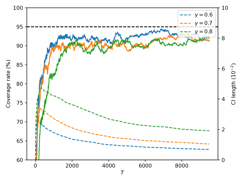
Figure 1: Empirical coverage rates (left) and CI lengths (right) of $\bar{Q}_{T}(s_{0},a_{0})$ against the number of iterations $T$ on a specific $(s_{0},a_{0})$. Both are obtained by averaging over 500 independent Q-learning trajectories. Black dashed line denotes the nominal coverage rate of 95%.

Comparison with previous (functional) CLTs.

Most CLT results consider linear SA which is non-applicable here (see Mou et al. [2020a, b] and references therein). The original result for Polyak-Ruppert averaging [Polyak and Juditsky, 1992, Moulines and Bach, 2011, Durmus et al., 2022] also doesn’t apply in our case because it assumes a locally strongly convex Lyapunov function—which is not known to exist for Q-learning. Konda and Tsitsiklis [1999] shows $\frac{{\bm{Q}}_{T}-{\bm{Q}}^{*}}{\sqrt{\eta_{T}}}\overset{d}{\to}{\mathcal{N}}({\bm{0}},\mathrm{Var})$ with $\mathrm{Var}=\frac{\lim_{T}}{\eta_{T}}{\mathbb{E}}({\bm{Q}}_{T}-{\bm{Q}}^{*})({\bm{Q}}_{T}-{\bm{Q}}^{*})^{\top}$ when we assume the limit involved exists. Mokkadem and Pelletier [2006] shows ${\bm{\phi}}_{T}(1)\overset{d}{\to}{\mathcal{N}}({\bm{0}},\mathrm{Var}_{\bm{Q}})$ under a similar Lipschitz condition Assumption 3.2.

To date, formal functional CLT results for SA are mainly based on the ODE approach [Abounadi et al., 2002, Borkar, 2009, Gadat et al., 2018, Borkar et al., 2021]. These works focus on the asymptotic behavior of the interpolated process connecting properly rescaled last iterates. An example interpolated process $\widetilde{{\bm{\phi}}}_{T}(\cdot)$ satisfies $\widetilde{{\bm{\phi}}}_{T}(0)=\frac{{\bm{Q}}_{T}-{\bm{Q}}^{*}}{\sqrt{\eta_{T}}}$ and $\widetilde{{\bm{\phi}}}_{T}(t_{k}^{T})=\frac{{\bm{Q}}_{T+k}-{\bm{Q}}^{*}}{\sqrt{\eta_{T+k}}}$ for a specific sequence $\{t_{k}^{T}\}_{k\geq 0}$ depending on the step size and satisfying $t_{0}^{T}=0$ and $\lim_{k}t_{k}^{T}=\infty$. This functional CLT result implies $\widetilde{{\bm{\phi}}}_{T}(\cdot)$ converges weakly to the solution of a specific SDE. Theorem 3.1 is different because it is concerned with the partial-sum process ${\bm{\phi}}_{T}(\cdot)$ and explicitly formulates the asymptotic variance $\mathrm{Var}_{\bm{Q}}$. Recent work studying statistical inference via SGD variants also provides functional CLTs for a similar partial-sum process [Lee et al., 2021, Li et al., 2022], given the loss function is smooth and strongly convex. However, those results don’t apply here since Q-learning doesn’t meet the underlying assumptions. Our functional CLT for the partial-sum process of Q-learning is novel.

3.1 Online Statistical Inference

The functional CLT opens a path towards statistical inference in RL. While traditional approaches estimate asymptotic variances in RL by batch-mean estimators [Chen et al., 2020a, Zhu et al., 2021] or bootstrapping [Hao et al., 2021], by contrast, the functional CLT allows us to construct an asymptotically pivotal statistic using the whole function ${\bm{\phi}}_{T}$. The inference method, known as random scaling, was originally designed for strongly convex optimization [Lee et al., 2021, Li et al., 2022].

Proposition 3.1.

The continuous mapping theorem together with Theorem 3.1 yields that with probability approaching one, $\int_{0}^{1}{\bm{\phi}}_{T}(r){\bm{\phi}}_{T}(r)^{\top}dr$ is invertible and

$$\begin{split}&{\bm{\phi}}_{T}(1)^{\top}\left(\int_{0}^{1}\bar{{\bm{\phi}}}_{T}(r)\bar{{\bm{\phi}}}_{T}(r)^{\top}\mathrm{d}r\right)^{-1}{\bm{\phi}}_{T}(1)\\ &\overset{d}{\to}{\bm{B}}_{D}(1)^{\top}\left(\int_{0}^{1}\bar{{\bm{B}}}_{D}(r)\bar{{\bm{B}}}_{D}(r)^{\top}\mathrm{d}r\right)^{-1}{\bm{B}}_{D}(1),\end{split}$$ (11)

where $\bar{{\bm{\phi}}}_{T}(r):={\bm{\phi}}_{T}(r)-r\cdot{\bm{\phi}}_{T}(1)$ and $\bar{{\bm{B}}}_{D}(r):={\bm{B}}_{D}(r)-r\cdot{\bm{B}}_{D}(1)$ for simplicity.

The left-hand side of (11) is a pivotal quantity involving samples and the unobservable parameter of interest ${\bm{Q}}^{*}$. The pivotal quantity can be constructed in a fully online fashion and thus is computationally efficient. The right-hand side of (11) is a known distribution whose quantiles can be computed via simulation [Kiefer et al., 2000, Abadir and Paruolo, 2002]. In this way, we don’t need a consistent estimator for the asymptotic variance in order to provide asymptotically valid confidence intervals for ${\bm{Q}}^{*}$, as are required by previous work [Hao et al., 2021, Shi et al., 2020, Khamaru et al., 2022]. As an illustration, Figure 1 shows the empirical coverage rates and confidence interval (CI) lengths on a random MDP with three values of $\gamma$. As $T$ increases, the empirical coverage rates increase rapidly, approaching $95\%$, and the CI lengths decay. More details are placed in Appendix J.

3.2 Proof Sketch

In the part, we provide a proof sketch of Theorem 3.1 to highlight our technical contributions. A full proof of Theorem 3.1 is provided in Appendix C.

Step 1: Error decomposition.

Let ${\mathbf{\Delta}}_{t}={\bm{Q}}_{t}-{\bm{Q}}^{*}$. Recall that the Q-learning update rule is (3). It follows that

$${\mathbf{\Delta}}_{t} =(1-\eta_{t}){\mathbf{\Delta}}_{t-1}+\eta_{t}\left[({\bm{r}}_{t}-{\bm{r}})+\gamma({\bm{P}}_{t}{\bm{V}}_{t-1}-{\bm{P}}{\bm{V}}^{*})\right]$$

$$=(1-\eta_{t}){\mathbf{\Delta}}_{t-1}+\eta_{t}\left[{\bm{Z}}_{t}+\gamma{\bm{P}}_{t}({\bm{V}}_{t-1}-{\bm{V}}^{*})\right],$$

where ${\bm{Z}}_{t}=({\bm{r}}_{t}-{\bm{r}})+\gamma({\bm{P}}_{t}-{\bm{P}}){\bm{V}}^{*}$ is the Bellman noise. Notice that ${\bm{P}}_{t}({\bm{V}}_{t-1}-{\bm{V}}^{*})=({\bm{P}}_{t}-{\bm{P}})({\bm{V}}_{t-1}-{\bm{V}}^{*})+{\bm{P}}({\bm{V}}_{t-1}-{\bm{V}}^{*})$. Using ${\bm{P}}{\bm{V}}_{t-1}={\bm{P}}^{\pi_{t-1}}{\bm{Q}}_{t-1}$ and ${\bm{P}}{\bm{V}}^{*}={\bm{P}}^{\pi^{*}}{\bm{Q}}^{*}$, we further have ${\bm{P}}({\bm{V}}_{t-1}-{\bm{V}}^{*})={\bm{P}}^{\pi_{t-1}}{\bm{Q}}_{t-1}-{\bm{P}}^{\pi^{*}}{\bm{Q}}^{*}=({\bm{P}}^{\pi_{t-1}}-{\bm{P}}^{\pi^{*}}){\bm{Q}}_{t-1}+{\bm{P}}^{\pi^{*}}\mbox{\boldmath$\Delta$\unboldmath}_{t-1}$. Putting the pieces together,

$${\mathbf{\Delta}}_{t}={\bm{A}}_{t}\mbox{\boldmath$\Delta$\unboldmath}_{t-1}+\eta_{t}\left[{\bm{Z}}_{t}+\gamma{\bm{Z}}_{t}^{\prime}+\gamma{\bm{Z}}_{t}^{\prime\prime}\right],$$

where ${\bm{A}}_{t}={\bm{I}}-\eta_{t}\bm{G},\bm{G}=\bm{I}-\gamma{\bm{P}}^{\pi^{*}},{\bm{Z}}_{t}^{\prime}=({\bm{P}}_{t}-{\bm{P}})({\bm{V}}_{t-1}-{\bm{V}}^{*})$, and ${\bm{Z}}_{t}^{\prime\prime}=({\bm{P}}^{\pi_{t-1}}-{\bm{P}}^{\pi^{*}}){\bm{Q}}_{t-1}$. Recursing the last equality gives

$${\mathbf{\Delta}}_{t}=\prod_{j=1}^{t}{\bm{A}}_{j}{\mathbf{\Delta}}_{0}+\sum_{j=1}^{t}\prod_{i=j+1}^{t}{\bm{A}}_{i}\eta_{j}\left({\bm{Z}}_{j}+\gamma{\bm{Z}}_{t}^{\prime}+\gamma{\bm{Z}}_{t}^{\prime\prime}\right).$$ (12)

In addition, using the general step size in Assumption 3.3, we can show $\frac{1}{\sqrt{T}}\sum_{t=1}^{T}{\mathbb{E}}\|{\mathbf{\Delta}}_{t}\|_{\infty}^{2}\to 0$ (in Theorem E.1).

Step 2: Partial-sum decomposition.

For simplicity, for any $T\geq j\geq 0$ we denote

$${\bm{A}}_{j}^{T}=\eta_{j}\sum_{t=j}^{T}\prod_{i=j+1}^{t}{\bm{A}}_{i}.$$ (13)

Setting ${\bm{\psi}}_{0}(r):=\frac{1}{\eta_{0}\sqrt{T}}({\bm{A}}_{0}^{{\lfloor Tr\rfloor}}-\eta_{0}{\bm{I}}){\mathbf{\Delta}}_{0}$ and plugging (12) into ${\bm{\phi}}_{T}(r)=\frac{1}{\sqrt{T}}\sum_{t=1}^{\lfloor Tr\rfloor}\mbox{\boldmath$\Delta$\unboldmath}_{t}$, yields

$${\bm{\phi}}_{T}(r)={\bm{\psi}}_{0}(r)+\frac{1}{\sqrt{T}}\sum_{j=1}^{{\lfloor Tr\rfloor}}{\bm{A}}_{j}^{{\lfloor Tr\rfloor}}\left({\bm{Z}}_{j}+\gamma{\bm{Z}}_{j}^{\prime}+\gamma{\bm{Z}}_{j}^{\prime\prime}\right)$$

$$={\bm{\psi}}_{0}(r)+\frac{1}{\sqrt{T}}\sum_{j=1}^{{\lfloor Tr\rfloor}}{\bm{G}}^{-1}{\bm{Z}}_{j}+\frac{1}{\sqrt{T}}\sum_{j=1}^{{\lfloor Tr\rfloor}}({\bm{A}}_{j}^{T}-{\bm{G}}^{-1}){\bm{Z}}_{j}$$

$$+\frac{\gamma}{\sqrt{T}}\sum_{j=1}^{{\lfloor Tr\rfloor}}{\bm{A}}_{j}^{T}{\bm{Z}}_{j}^{\prime}+\frac{1}{\sqrt{T}}\sum_{j=1}^{{\lfloor Tr\rfloor}}({\bm{A}}_{j}^{{\lfloor Tr\rfloor}}-{\bm{A}}_{j}^{T})\left[{\bm{Z}}_{j}+\gamma{\bm{Z}}_{j}^{\prime}\right]$$

$$+\frac{\gamma}{\sqrt{T}}\sum_{j=1}^{{\lfloor Tr\rfloor}}{\bm{A}}_{j}^{T}{\bm{Z}}_{j}^{\prime\prime}:=\sum_{i=0}^{5}{\bm{\psi}}_{i}(r).$$ (14)

Step 3: Establish the functional CLT.

To measure the distance between random functions, we define $\|{\bm{\psi}}\|_{\sup}=\sup_{r\in[0,1]}\|{\bm{\psi}}(r)\|_{\infty}$. The standard martingale functional CLT [Hall and Heyde, 2014, Jirak, 2017] implies ${\bm{\psi}}_{1}(\cdot)\overset{w}{\to}\mathrm{Var}_{\bm{Q}}^{1/2}{\bm{B}}_{D}(\cdot)$. To complete the proof, it suffice to show $\|{\bm{\phi}}_{T}-{\bm{\psi}}_{1}\|_{\sup}=o_{{\mathbb{P}}}(1)$ which is implied by $\|{\bm{\psi}}_{i}\|_{\sup}=o_{{\mathbb{P}}}(1)$ for $i=0,2,3,4,5$.

By Lemma 1 in [Polyak and Juditsky, 1992], we know $\sup_{T\geq j\geq 0}\|{\bm{A}}_{j}^{T}\|_{\infty}\leq C_{0}$ and $\lim_{T\to\infty}\frac{1}{T}\sum_{j=1}^{T}\|{\bm{A}}_{j}^{T}-{\bm{G}}^{-1}\|_{2}=0$. Then it is obvious $\|{\bm{\psi}}_{0}\|_{\sup}=o_{{\mathbb{P}}}(1)$. Noting that ${\bm{Z}}_{j},{\bm{Z}}_{j}^{\prime}$ are martingale differences, we can show ${\mathbb{E}}\|{\bm{\psi}}_{i}\|_{\sup}^{2}=o(1)$ for $i=2,3$ by Doob’s inequality.

By definition of greedy policies $\pi^{*}$ and $\pi_{t-1}$, we know ${\bm{P}}^{\pi^{*}}{\bm{Q}}_{t-1}\leq{\bm{P}}^{\pi_{t-1}}{\bm{Q}}_{t-1}$ and ${\bm{P}}^{\pi_{t-1}}{\bm{Q}}^{*}\leq{\bm{P}}^{\pi^{*}}{\bm{Q}}^{*}$, which implies $\|{\bm{Z}}_{t}^{\prime\prime}\|_{\infty}=\|({\bm{P}}^{\pi_{t-1}}-{\bm{P}}^{\pi^{*}}){\bm{Q}}_{t-1}\|_{\infty}\leq\|({\bm{P}}^{\pi_{t-1}}-{\bm{P}}^{\pi^{*}})\mbox{\boldmath$\Delta$\unboldmath}_{t-1}\|_{\infty}\leq L\|\mbox{\boldmath$\Delta$\unboldmath}_{t-1}\|_{\infty}^{2}$ from Assumption 3.2. Then ${\mathbb{E}}\|{\bm{\psi}}_{5}\|_{\sup}\leq\frac{LC_{0}}{\sqrt{T}}\sum_{t=1}^{T}{\mathbb{E}}\|\mbox{\boldmath$\Delta$\unboldmath}_{t}\|_{\infty}^{2}\to 0$.

The most challenging step is to show $\|{\bm{\psi}}_{4}\|_{\sup}=o_{{\mathbb{P}}}(1)$. Notice that ${\bm{\psi}}_{4}$ is a weighted sum of martingale differences, ${\bm{Z}}_{j}+\gamma{\bm{Z}}_{j}^{\prime}$, with the coefficients varying in $r$ such that we can’t apply Doob’s inequality. To deal with this issue, we relate ${\bm{\psi}}_{4}$ to an autoregressive sequence indexed by $k\in[T]$ and analyze the maximum over $k$ directly. More specifically, we can show

$$\|{\bm{\psi}}_{4}\|_{\sup}\precsim\sup_{k\in[T]}\left\|\frac{1}{\sqrt{T}\eta_{k+1}}\sum_{j=1}^{k}\prod_{i=j+1}^{k}{\bm{A}}_{i}\eta_{j}({\bm{Z}}_{j}+\gamma{\bm{Z}}_{j}^{\prime})\right\|.$$

Previous results Lee et al. [2021], Li et al. [2022] do not apply here, since they require $\bm{G}=\bm{I}-\gamma{\bm{P}}^{\pi^{*}}$ to be positive semidefinite, which isn’t our case. Noticing that all eigenvalues of $\bm{G}$ have nonnegative real parts, we provide a novel analysis of the right-hand side in Lemma D.1, showing it is indeed $o_{{\mathbb{P}}}(1)$ under Assumption 3.1. This is one of our technical contributions.

Remark 3.1.

If we consider policy evaluation (so that $\pi_{t}$ remains unchanged and ${\bm{\psi}}_{5}$ disappears), ${\bm{\psi}}_{4}$ is still present. Showing $\|{\bm{\psi}}_{4}\|_{\sup}=o_{{\mathbb{P}}}(1)$ is required even for linear SA.

4 INFORMATION-THEORETIC LOWER BOUND

The standard CLT implies $\bar{{\bm{Q}}}_{T}$ is a $\sqrt{T}$-consistent estimate for ${\bm{Q}}^{*}$. It is of theoretical interest to investigate whether or not $\bar{{\bm{Q}}}_{T}$ is asymptotically efficient. In parametric statistics [Lehmann and Casella, 2006], the Cramer-Rao lower bound assesses the hardness of estimating a target parameter $\beta(\theta)$ in a parametric model ${\mathcal{P}}_{\theta}$ indexed by parameter $\theta$. Any unbiased estimator whose variance achieves the Cramer-Rao lower bound is viewed as optimal and efficient. The concept of Cramer-Rao lower bounds can be extended to possibly biased but asymptotically unbiased estimators and also to nonparametric statistical models where the dimension of the parameter $\theta$ is infinity [Van der Vaart, 2000, Tsiatis, 2006].

The semiparametric model.

In our case, the transition kernel $\{P(\cdot|s,a)\}_{s,a}$ is specified by $D$ parametric distributions on ${\mathcal{D}}$, while the random reward $\{R(s,a)\}_{s,a}$ is fully nonparametric because the $R(s,a)$ are not assumed to come from finite-dimensional models. Hence, to derive an extended Cramer-Rao lower bound for $Q^{*}$ estimation, we need to enter the world of semiparametric statistics. In particular, our MDP model $\mathcal{M}=({\mathcal{S}},{\mathcal{A}},\gamma,P,R,r)$ has parameter $\theta=(P,R)$. Our parameter of interest is $\beta(\theta)={\bm{Q}}^{*}$. At iteration $t$, we observe the random rewards and empirical transitions for each $(s,a)$ and concatenate them into ${\bm{r}}_{t}\in{\mathbb{R}}^{D}$ and ${\bm{P}}_{t}\in{\mathbb{R}}^{D\times S}$. The distribution of ${\bm{P}}_{t}$ is determined by its expectation ${\bm{P}}={\mathbb{E}}{\bm{P}}_{t}$, which belongs to

$$\begin{split}{\mathcal{P}}_{P}:&=\left\{{\bm{P}}\in{\mathbb{R}}^{D\times S}:P(s^{\prime}|s,a)\geq 0,\forall(s,a,s^{\prime})\right.\\ &\text{and}\left.\sum_{s^{\prime}\in{\mathcal{S}}}P(s^{\prime}|s,a)=1,\forall(s,a)\right\},\end{split}$$ (15)

while $R$ is nonparametric and belongs to

$${\mathcal{P}}_{R}=\left\{\{R(s,a)\}_{s,a}:{\mathbb{E}}R(s,a)=r(s,a),\forall(s,a)\right\}.$$

According to the generative model, the ${\bm{r}}_{t}$ and ${\bm{P}}_{t}$ are mutually independent and also independent of the historical data. Let ${\mathcal{D}}=\{({\bm{r}}_{t},{\bm{P}}_{t})\}_{t\in[T]}$ contain the $T$ samples generated as described above.

Semiparametric efficiency lower bound.

Tsiatis [2006] has argued that regular asymptotically linear (RAL) estimators provide a good tradeoff between expressivity and tractability. In RL, RAL estimators are widely considered in off-policy evaluation problems [Kallus and Uehara, 2020].

Definition 4.1 (Regular estimator).

Denote the distribution of ${\bm{r}}_{t}$ and ${\bm{P}}_{t}$ by ${\mathcal{L}}({\bm{r}})$ and ${\mathcal{L}}({\bm{P}})$. For any given $T$, let ${\mathcal{L}}_{T}({\bm{r}})$ and ${\mathcal{L}}_{T}({\bm{P}})$ be the perturbed distributions of ${\mathcal{L}}({\bm{r}})$ and ${\mathcal{L}}({\bm{P}})$ which are consistent in the sense that they converge to ${\mathcal{L}}({\bm{r}})$ and ${\mathcal{L}}({\bm{P}})$ when $T$ goes infinity. Let $\widehat{{\bm{Q}}}_{T}$ be any estimator of ${\bm{Q}}^{*}$ computed from ${\mathcal{D}}$. Let ${\bm{Q}}^{*}_{T}$ be the true optimal Q-value function when rewards and transition probabilities are generated i.i.d. from ${\mathcal{L}}_{T}({\bm{r}})$ and ${\mathcal{L}}_{T}({\bm{P}})$. We say $\widehat{{\bm{Q}}}_{T}$ is a regular estimator of ${\bm{Q}}^{*}$ if $\sqrt{T}(\widehat{{\bm{Q}}}_{T}-{\bm{Q}}^{*}_{T})$ weakly converges to a random variable that depends only on ${\mathcal{L}}({\bm{r}})$ and ${\mathcal{L}}({\bm{P}})$, when samples are distributed according to the probability measure $({\mathcal{L}}_{T}({\bm{r}}),{\mathcal{L}}_{T}({\bm{P}}))$.

Remark 4.1.

Informally speaking, an estimator is regular if its limiting distribution is unaffected by local changes in the data-generating process. The assumption of regularity excludes super-efficient estimators, whose asymptotic variance can be smaller than the Cramer-Rao lower bound for some parameter values, but which perform poorly in the neighborhood of points of super-efficiency. We refer interested readers to Section 3.1 in [Tsiatis, 2006] for a detailed exposition.

Definition 4.2 (Regular asymptotically linear).

Let $\widehat{{\bm{Q}}}_{T}\in{\mathbb{R}}^{D}$ be a measurable random function of ${\mathcal{D}}=\{({\bm{r}}_{t},{\bm{P}}_{t})\}_{t\in[T]}$. We say that $\widehat{{\bm{Q}}}_{T}$ is regular asymptotically linear (RAL) for ${\bm{Q}}^{*}$ if it is regular and asymptotically linear with a measurable random function ${\bm{\phi}}({\bm{r}}_{t},{\bm{P}}_{t})\in{\mathbb{R}}^{D}$ such that

$$\sqrt{T}(\widehat{{\bm{Q}}}_{T}-{\bm{Q}}^{*})=\frac{1}{\sqrt{T}}\sum_{t=1}^{T}{\bm{\phi}}({\bm{r}}_{t},{\bm{P}}_{t})+o_{{\mathbb{P}}}(1).$$

Here ${\bm{\phi}}(\cdot,\cdot)$ is referred to as an influence function, and it satisfies ${\mathbb{E}}{\bm{\phi}}({\bm{r}}_{t},{\bm{P}}_{t})={\bm{0}}$ and ${\mathbb{E}}{\bm{\phi}}({\bm{r}}_{t},{\bm{P}}_{t}){\bm{\phi}}({\bm{r}}_{t},{\bm{P}}_{t})^{\top}$.

Theorem 4.1.

Given the dataset ${\mathcal{D}}=\{({\bm{r}}_{t},{\bm{P}}_{t})\}_{t\in[T]}$, for any RAL estimator $\widehat{{\bm{Q}}}_{T}$ of ${\bm{Q}}^{*}$ computed from ${\mathcal{D}}=\{({\bm{r}}_{t},{\bm{P}}_{t})\}_{t\in[T]}$, its variance satisfies

$$\lim_{T\to\infty}T{\mathbb{E}}(\widehat{{\bm{Q}}}_{T}-{\bm{Q}}^{*})(\widehat{{\bm{Q}}}_{T}-{\bm{Q}}^{*})^{\top}\succeq\mathrm{Var}_{\bm{Q}},$$

where ${\bm{A}}\succeq{\bm{B}}$ means ${\bm{A}}-{\bm{B}}$ is positive semidefinite and $\mathrm{Var}_{\bm{Q}}$ is given in (10).

By Definition 4.2, any influence function determines an asymptotic linear estimator for ${\bm{Q}}^{*}$. The semiparametric efficiency bound in Theorem 4.1 gives us a concrete target in the construction of the influence function. If we can find an influence function that achieves the bound, we know that it is the most efficient among all RAL estimators. Fortunately, Theorem 4.2 implies that $\bar{{\bm{Q}}}_{T}$ is the most efficient estimator among all RAL estimators with the efficient influence function $({\bm{I}}-\gamma{\bm{P}}^{\pi^{*}})^{-1}{\bm{Z}}_{t}$. It also implies that for any fixed $r\in[0,1]$, ${\bm{\phi}}_{T}(r)=\sqrt{r}\cdot\sqrt{\lfloor Tr\rfloor}(\bar{{\bm{Q}}}_{\lfloor Tr\rfloor}-{\bm{Q}}^{*})$ has the optimal asymptotic variance (scaled by a factor $\sqrt{r}$). Proofs are provided in Appendix G.

Theorem 4.2.

Under Assumptions 3.1, 3.2 and 3.3, the averaged Q-learning iterate $\bar{{\bm{Q}}}_{T}$ is a RAL estimator for ${\bm{Q}}^{*}$. In particular, we have the following decomposition

$$\sqrt{T}\left(\bar{{\bm{Q}}}_{T}-{\bm{Q}}^{*}\right)=\frac{1}{\sqrt{T}}\sum_{t=1}^{T}({\bm{I}}-\gamma{\bm{P}}^{\pi^{*}})^{-1}{\bm{Z}}_{t}+o_{{\mathbb{P}}}(1),$$

where ${\bm{Z}}_{t}=({\bm{r}}_{t}-{\bm{r}})+\gamma({\bm{P}}_{t}-{\bm{P}}){\bm{V}}^{*}$ is the Bellman noise at iteration $t$.

5 INSTANCE-DEPENDENT NONASYMPTOTIC CONVERGENCE

In the section, we explore the nonasymptotic behavior of averaged Q-learning, i.e., we study the dependence of ${\mathbb{E}}\|\bar{{\bm{Q}}}_{T}-{\bm{Q}}^{*}\|_{\infty}$ on finite $T$ and $(1-\gamma)^{-1}$.

Theorem 5.1.

Let Assumptions 3.2 hold and $0\leq R(s,a)\leq 1$ for all $(s,a)\in{\mathcal{S}}\times{\mathcal{A}}$. When $D$ is larger than a universal constant,

• If $\eta_{t}=t^{-\alpha}$ with $\alpha\in(0.5,1)$ for $t\geq 1$ and $\eta_{0}=1$, it follows that for all $T\geq 1$, ${\mathbb{E}}\|\bar{{\bm{Q}}}_{T}-{\bm{Q}}^{*}\|_{\infty}=$

  $$\begin{split}&{\mathcal{O}}\left(\sqrt{\|\mathrm{diag}(\mathrm{Var}_{\bm{Q}})\|_{\infty}}\sqrt{\frac{\ln D}{T}}+\frac{\sqrt{\ln D}}{(1-\gamma)^{3}}\frac{1}{T^{1-\frac{\alpha}{2}}}\right)\\ &\qquad+\widetilde{{\mathcal{O}}}\left(\frac{1}{(1-\gamma)^{3+\frac{2}{1-\alpha}}}\frac{1}{T}+\frac{\gamma L}{(1-\gamma)^{4+\frac{1}{1-\alpha}}}\frac{1}{T^{\alpha}}\right).\end{split}$$

• If $\eta_{t}=\frac{1}{1+(1-\gamma)t}$, it follows that for all $T\geq 1$, ${\mathbb{E}}\|\bar{{\bm{Q}}}_{T}-{\bm{Q}}^{*}\|_{\infty}=$

  $${\mathcal{O}}\left(\sqrt{\frac{\|\mathrm{Var}({\bm{Z}})\|_{\infty}}{(1-\gamma)^{2}}}\sqrt{\frac{\ln D}{T}}\right)+{\widetilde{{\mathcal{O}}}}\left(\frac{L}{(1-\gamma)^{6}}\frac{1}{T}\right).$$

Here ${\widetilde{{\mathcal{O}}}}(\cdot)$ hides polynomial dependence on $\alpha,L$ and logarithmic factors (i.e., $\ln D$ and $\ln T$).

Instance-dependent behavior.

For the polynomial step size, Theorem 5.1 shows that the instance-dependent term ${\mathcal{O}}(\sqrt{\|\mathrm{diag}(\mathrm{Var}_{\bm{Q}})\|_{\infty}}\sqrt{\frac{\ln D}{T}})$ dominates the $\ell_{\infty}$ error, which matches the instance-dependent lower bound established by Khamaru et al. [2021b] given a sufficiently large $T$. To the best of our knowledge, this is the first finite-sample analysis of averaged Q-learning in the $\ell_{\infty}$-norm showing instance-dependent optimality. However, for the linearly rescaled step size, we see that ${\mathcal{O}}\left(\sqrt{\frac{\|\mathrm{Var}({\bm{Z}})\|_{\infty}}{(1-\gamma)^{2}}}\sqrt{\frac{\ln D}{T}}\right)$ is the dominant factor, which is larger because we have

$$\|\mathrm{diag}(\mathrm{Var}_{\bm{Q}})\|_{\infty} \overset{(a)}{\leq}\|({\bm{I}}-\gamma{\bm{P}}^{\pi^{*}})^{-1}\|_{\infty}^{2}\|\mathrm{Var}({\bm{Z}})\|_{\infty}$$

$$\overset{(b)}{\leq}\frac{1}{(1-\gamma)^{2}}\|\mathrm{Var}({\bm{Z}})\|_{\infty},$$

where $(a)$ uses $\|\mathrm{diag}({\bm{A}}{\bm{V}}{\bm{A}}^{\top})\|_{\infty}\leq\|{\bm{V}}\|_{\infty}\|{\bm{A}}\|_{\infty}^{2}$ for any diagonal matrix ${\bm{V}}$ (see Lemma F.2) and $(b)$ uses $\|({\bm{I}}-\gamma{\bm{P}}^{\pi^{*}})^{-1}\|_{\infty}\leq(1-\gamma)^{-1}$. Hence, the linearly rescaled step size doesn’t match the instance-dependent lower bound. It might be true because the linearly rescaled step size doesn’t satisfy Assumption 3.3, implying that (22) does not necessarily hold for it.

Comparison with variance-reduced Q-learning.

Under the same assumptions, Khamaru et al. [2021b] analyzed a variance-reduced variant of Q-learning that also achieves instance-dependent optimality with the following guarantee:

$${\mathbb{E}}\|\widehat{{\bm{Q}}}_{T}-{\bm{Q}}^{*}\|_{\infty}=$$

$${\mathcal{O}}\left(\sqrt{\|\mathrm{diag}(\mathrm{Var}_{\bm{Q}})\|_{\infty}}\sqrt{\frac{\ln D}{T}}\right)+{\widetilde{{\mathcal{O}}}}\left(\frac{1}{(1-\gamma)^{2}}\frac{1}{T}\right),$$

which has a better nonleading term than averaged Q-learning. This might somewhat explain the finding of Khamaru et al. [2021a] that averaging can be sub-optimal in the nonasymptotic regime with limited samples. However, the dominant terms are equal, implying that averaging is still powerful and efficient in the asymptotic regime. Instance-dependent convergence with a variance structure in the dominant term has also been found for other settings; please see Appendix A.

Worst-case behavior.

The instance-dependent bound provides more information about the convergence rate. Previous works [Azar et al., 2013, Li et al., 2020a] imply the worst-case bound $\|\mathrm{diag}(\mathrm{Var}_{\bm{Q}})\|_{\infty}={\mathcal{O}}((1-\gamma)^{-3})$. Such a dependence on $(1-\gamma)^{-1}$ is tight, because Khamaru et al. [2021b] constructs a family of MDPs parameterized by $\lambda\geq 0$ where $\|\mathrm{diag}(\mathrm{Var}_{\bm{Q}})\|_{\infty}=\Theta((1-\gamma)^{-3+\lambda})$. When plugging in the worst-case bound, we find that for polynomial step sizes and for sufficiently small $\varepsilon$, averaged Q-learning already achieves the optimal minimax sample complexity ${\widetilde{{\mathcal{O}}}}\left(\frac{D}{(1-\gamma)^{3}\varepsilon^{2}}\right)$ established by Azar et al. [2013]. Wainwright [2019c] uses a variance-reduced variant of Q-learning to achieve the optimality, but the algorithm requires an additional collection of i.i.d. samples at each outer loop to obtain an Monte Carlo approximation of the population Bellman operator (5). Our results show that a simple average is sufficient to guarantee optimality. Moreover, the computation of $\bar{{\bm{Q}}}_{T}$ is fully online with no additional samples needed.

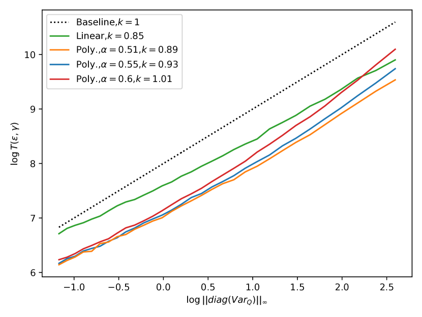
Figure 2: Log-log plots of the sample complexity $T(\varepsilon,\gamma)$ versus the asymptotic variance $\|\mathrm{diag}(\mathrm{Var}_{\bm{Q}})\|_{\infty}$.

Confirming the theoretical predictions.

We provide numerical experiments to illustrate instance-adaptivity as well as the worst-case behavior delineated in Theorem 5.1. We focus on the sample complexity $T(\varepsilon,\gamma)=\inf\{T:{\mathbb{E}}\|\bar{{\bm{Q}}}_{T}-{\bm{Q}}^{*}\|_{\infty}\leq\varepsilon\}$ for $\varepsilon=10^{-4}$. We conduct $10^{3}$ independent trials in a random MDP to compute $T(\varepsilon,\gamma)$ for different values of $\gamma\in\Gamma$ and two step sizes. We plot the least-squares fits, $\{(\log\|\mathrm{diag}(\mathrm{Var}_{\bm{Q}})\|_{\infty},\log T(\varepsilon,\gamma))\}_{\gamma\in\Gamma}$, and provide the slopes $k$ of these lines in the legend. Further details are provided in Appendix J. At a high level, we see that averaged Q-learning produces sample complexity that is well predicted by our theory—all the slopes are no larger than the theoretical limit $k$ predicted by our theory.

Proof Sketch.

The proof idea of Theorem 5.1 is based on that of Theorem 3.1. Notice that $\bar{{\bm{Q}}}_{T}-{\bm{Q}}^{*}=\frac{1}{T}\sum_{t=1}^{T}\mbox{\boldmath$\Delta$\unboldmath}_{t}=\frac{1}{\sqrt{T}}{\bm{\phi}}_{T}(1)$. From (14), we know that

$${\mathbb{E}}\|\bar{{\bm{Q}}}_{T}-{\bm{Q}}^{*}\|_{\infty}={\mathbb{E}}\left\|\frac{{\bm{\phi}}_{T}(1)}{\sqrt{T}}\right\|_{\infty}\leq\frac{\sum_{i\neq 4}{\mathbb{E}}\left\|{\bm{\psi}}_{i}(1)\right\|_{\infty}}{\sqrt{T}}.$$

Bounding the term of $i=0$ is easy since it’s deterministic. Because ${\bm{\psi}}_{i}(1)(i=1,2,3)$ is a weighted sum of martingale differences, we use the variance-aware multi-dimensional Freedman’s inequality (in Lemma H.1) to analyze its expectation under $\ell_{\infty}$-norm. The instance-dependent dominant term comes from the variance term for ${\mathbb{E}}\|{\bm{\psi}}_{1}(1)\|_{\infty}$. Analyzing the variance of ${\bm{\psi}}_{2}(1)$ is quite challenging since it relies on $\frac{1}{T}\sum_{j=1}^{T}\|{\bm{A}}_{j}^{T}-\bm{G}^{-1}\|_{\infty}^{2}$ with ${\bm{A}}_{j}^{T}$ defined in (13). We then bound that quantity in terms of $\alpha,1-\gamma$ and $T$ in Lemma C.4. Finally, due to $\|{\bm{\psi}}_{5}(1)\|_{\infty}\leq L\|\mbox{\boldmath$\Delta$\unboldmath}_{t}\|_{\infty}^{2}$, bounding ${\mathbb{E}}\|{\bm{\psi}}_{5}(1)\|_{\infty}$ is reduced to bound ${\mathbb{E}}\|\mbox{\boldmath$\Delta$\unboldmath}_{t}\|_{\infty}^{2}$ for all $t\geq 0$, which can be given by a similar argument from Wainwright [2019b]. Putting all pieces together completes the proof; the detailed proof is in Appendix F.

6 RELAXATION OF THE LIPSCHITZ CONDITION

Both our asymptotic and nonasymptotic analysis rely on the Lipschitz condition in Assumption 3.2. That condition is essentially equivalent to assuming a unique optimal policy. It turns out that, once regularized by entropy, the (regularized) optimal policy is naturally unique. In the following, we show that entropy-regularized Q-learning enjoys a similar functional CLT and instance-dependent bounds without Assumption 3.2.

Entropy-regularized Q-learning uses the following matrix-form update rule,

$${\widetilde{{\bm{Q}}}}_{t}=(1-\eta_{t}){\widetilde{{\bm{Q}}}}_{t-1}+\eta_{t}\widetilde{{\mathcal{T}}}_{t}{\widetilde{{\bm{Q}}}}_{t-1},$$ (16)

where

$$\widetilde{{\mathcal{T}}}_{t}({\bm{Q}})(s,a)={\bm{r}}_{t}(s,a)+\gamma({\bm{P}}_{t}{\mathcal{L}}_{\lambda}{\bm{Q}})(s_{t})$$ (17)

is a soft version of the empirical Bellman operator $\widehat{{\mathcal{T}}}$. The nonlinear operator ${\mathcal{L}}_{\lambda}(\cdot):{\mathbb{R}}^{D}\to{\mathbb{R}}^{S}$ is a soft version of a hard max, with regularization coefficient $\lambda$. It is defined by

$$({\mathcal{L}}_{\lambda}{\bm{Q}})(s):=\max_{\pi\in\Pi}{\mathbb{E}}_{a\sim\pi(\cdot|s)}\left[Q(s,a)-\lambda\log\pi(a|s)\right].$$

Let ${\bm{Q}}_{\lambda}^{*}$ denote the unique fixed point of the regularized Bellman equation ${\bm{Q}}_{\lambda}^{*}={\bm{r}}+\gamma{\bm{P}}{\mathcal{L}}_{\lambda}{\bm{Q}}_{\lambda}^{*}$ and let $\pi_{\lambda}^{*}$ be the unique optimal policy.

Theorem 6.1.

Define $\{\widetilde{{\bm{Q}}}_{t}\}_{t\geq 0}$ in (16). The corresponding partial-sum process is ${\widetilde{{\bm{\phi}}}}_{T}(r):=\frac{1}{\sqrt{T}}\sum_{t=1}^{{\lfloor Tr\rfloor}}({\widetilde{{\bm{Q}}}}_{t}-{\bm{Q}}_{\lambda}^{*})$. Under Assumptions 3.1 and 3.3,

$${\widetilde{{\bm{\phi}}}}_{T}(\cdot)\overset{w}{\to}\widetilde{\mathrm{Var}}_{\bm{Q}}^{1/2}{\bm{B}}_{D}(\cdot),$$

where $\widetilde{\mathrm{Var}}_{\bm{Q}}$ is the asymptotic matrix defined by

$$\widetilde{\mathrm{Var}}_{\bm{Q}}:=({\bm{I}}-\gamma{\bm{P}}^{\pi_{\lambda}^{*}})^{-1}\mathrm{Var}({\widetilde{{\bm{Z}}}})({\bm{I}}-\gamma{\bm{P}}^{\pi_{\lambda}^{*}})^{-\top}.$$

with ${\widetilde{{\bm{Z}}}}\overset{d.}{=}{\widetilde{{\bm{Z}}}}_{t}=({\bm{r}}_{t}-{\bm{r}})+\gamma({\bm{P}}_{t}-{\bm{P}}){\mathcal{L}}_{\lambda}{\bm{Q}}_{\lambda}^{*}$ the regularized Bellman noise.

Theorem 6.2.

Under Assumptions 3.1 and 3.3, when the two step sizes are considered, ${\mathbb{E}}\|\frac{1}{T}\sum_{t=1}^{T}{\widetilde{{\bm{Q}}}}_{t}-{\bm{Q}}_{\lambda}^{*}\|_{\infty}$ has similar bounds as in Theorem 5.1 except that we replace $\mathrm{Var}_{\bm{Q}},L$ with $\widetilde{\mathrm{Var}}_{\bm{Q}}$ and $\frac{1}{\lambda}$.

We note that the two theorems in this section can be proved via an almost identical argument as Theorem 3.1 and 5.1, since Assumption 3.2 is naturally satisfied with $L=\frac{1}{\lambda}$ for entropy-regularized Q-learning (see Appendix I). Actually, our proof is applicable to a class of nonlinear SAs. Second, due to the bias introduced by entropy, the instance-dependent factor changes from $\mathrm{Var}_{\bm{Q}}$ to $\widetilde{\mathrm{Var}}_{\bm{Q}}$ and $\frac{1}{T}\sum_{t=1}^{T}{\widetilde{{\bm{Q}}}}_{t}$ converges to ${\bm{Q}}_{\lambda}^{*}$ instead of ${\bm{Q}}^{*}$ in expectation. Finally, note that these results provide a new argument for the benefits of entropy regularization; it smooths the Bellman operator and weakens the assumptions required for asymptotic analysis. It is supplementary to previous efforts that shows entropy regularization aids exploration [Fox et al., 2016], encourages robust optimal policies [Eysenbach and Levine, 2021], induces a smoother landscape [Ahmed et al., 2019], and hastens the convergence of RL algorithms [Cen et al., 2022].

7 DISCUSSION

We have studied the asymptotic and nonasymptotic convergence of averaged Q-learning, establishing its statistical efficiency. We first established a functional central limit theorem, showing that the standardized partial-sum process converges weakly to a rescaled Brownian motion, a result which can serve as an underpinning for the development of statistical inference methods for RL. We then established a semiparametric efficiency lower bound for ${\bm{Q}}^{*}$ estimation, showing that the averaged iterate $\bar{{\bm{Q}}}_{T}$ is the most efficient RAL estimator in the sense of having the smallest asymptotic variance. Finally, we presented the first finite-sample error analysis of ${\mathbb{E}}\|\bar{{\bm{Q}}}_{T}-{\bm{Q}}^{*}\|_{\infty}$ in the $\ell_{\infty}$-norm for both linearly rescaled and polynomial step sizes. We showed that averaged Q-learning achieves the same instance-dependent optimality and worst-case optimality as previous variance-reduced algorithms [Khamaru et al., 2021b, Wainwright, 2019c] under a Lipschitz condition.

Some open problems remain. On the one hand, with the Lipschitz condition, it’s unclear whether averaged Q-learning with linearly rescaled step sizes can match the instance-dependent lower bound. Additionally, we suspect that the dependence on $(1-\gamma)^{-1}$ of the nonleading terms in Theorem 5.1 is loose and speculate it can be improved by finer analysis. On the other hand, without the Lipschitz condition, it is not clear whether averaged Q-learning still achieves the optimal instance-dependent bound. Finally, previous analysis [Kozuno et al., 2022] shows the last-iterate entropy-regularized Q-learning is minimax optimal. It is also unknown whether the averaged iterates of entropy-regularized Q-learning achieve the optimal instance-dependent bound.

Appendix A RELATED WORK

Due to the rapidly growing literature on Q-learning, we review only the theoretical results that are most relevant to our work. Interested readers can check references therein for more information.

Asymptotic normality in RL.

Establishing asymptotic normality of an estimator permits statistical inference and the quantification of uncertainty. Existing work on statistical inference for Q-learning has focused mainly on the off-policy evaluation (OPE) problem, where one aims to estimate the value function of a given policy using pre-collected data. In this setting, a parametric Cramer–Rao lower bound has been established by Jiang and Li [2016], and asymptotic efficiency has been established for certain estimators using linear approximation [Uehara et al., 2020, Hao et al., 2021, Yin and Wang, 2020, Mou et al., 2020a] or bootstrapping [Hao et al., 2021]. Further inferential work includesthe asymptotic analysis of multi-stage algorithms [Luckett et al., 2019, Shi et al., 2020], asymptotic behavior of robust estimators [Yang et al., 2021], and work by Kallus and Uehara [2020] on a semiparametric doubly robust estimator.

In contradistinction to existing work, we establish a functional central limit theorem that captures the weak convergence of the whole trajectory rather than its endpoint. Such functional results have not been presented previously in the RL literature. Furthermore, we supplement these upper bounds with a semiparametric efficiency lower bound which additionally considers the randomness of rewards. We also show that averaged Q-learning is the most efficient RAL estimator vis-a-vis this lower bound.

Sample complexity for Q-learning.

For the goal of obtaining an $\varepsilon$-accurate estimate of the optimal Q-function in a $\gamma$-discounted MDP in the presence of a generative model, model-based Q-value-iteration has been shown to achieve optimal minimax sample complexity ${\widetilde{{\mathcal{O}}}}\left(\frac{D}{\varepsilon^{2}(1-\gamma)^{3}}\right)$ [Azar et al., 2013, Agarwal et al., 2020, Li et al., 2020a]. In the model-free context, Wainwright [2019b] showed empirically that classical Q-learning suffers from at least worst-case fourth-order scaling in $(1-\gamma)^{-1}$ in sample complexity. A complexity bound of ${\widetilde{{\mathcal{O}}}}\left(\frac{D}{\varepsilon^{2}(1-\gamma)^{5}}\right)$ has been provided [Wainwright, 2019b, Chen et al., 2020b]; this is far from the optimal though better than previous efforts [Even-Dar et al., 2003, Beck and Srikant, 2012].  Li et al. [2021a] gave a sophisticated analysis showing the complexity of Q-learning is ${\widetilde{{\mathcal{O}}}}\left(\frac{D}{\varepsilon^{2}(1-\gamma)^{4}}\right)$ and provided a matching lower bound to confirm its sharpness.  Wainwright [2019c], Khamaru et al. [2021b] introduced a variance-reduced variant of Q-learning [Gower et al., 2020] that achieves the optimal sample complexity and instance complexity. Our results show that a simple average over all history $Q_{t}$ is sufficient to guarantee the same optimality. The averaged method is fully online without requiring additional samples and storage space.

Instance-dependent convergence in RL.

Recent years have witnessed new instance-specific bounds, where an instance-dependent functional of a variance structure appears as the dominant term on stochastic errors. Unlike global minimax bounds which are worst-case in nature, instance-specific bounds help identify the difficulty of estimation case by case. Such bounds have been established for policy evaluation in the tabular setting [Pananjady and Wainwright, 2020, Khamaru et al., 2021a, Li et al., 2020a] or with linear function approximation [Li et al., 2021b] and for optimal value function estimation [Yin and Wang, 2021]. The most related work to ours is by Khamaru et al. [2021b], who show that a variance-reduced variant of Q-learning achieves the instance-dependent optimality after identifying an instance-dependent lower bound for $Q^{*}$ estimation. By contrast, our result shows that a simple average is sufficient to yield optimality.

Nonlinear stochastic approximation.

Q-learning has also been studied through the lens of nonlinear stochastic approximation. From this general point of view, asymptotic convergence has been provided [Tsitsiklis, 1994, Borkar and Meyn, 2000]. On the nonasymptotic side, Q-learning is studied either in the synchronous setting [Shah and Xie, 2018, Wainwright, 2019b, Chen et al., 2020b] or the asynchronous setting where only one sample from current state-action pair is available at a time [Qu and Wierman, 2020, Li et al., 2020b, Chen et al., 2021]. The sample complexities obtained therein are far from optimal. Others consider Q-learning with linear function approximation in the $\ell_{2}$-norm [Melo et al., 2008, Chen et al., 2019]. Asymptotic convergence of averaged Q-learning has been studied by Lee and He [2019a, b] via the ODE (ordinary differential equation) approach. Our results are complementary to these results, including asymptotic statistical properties and finite-sample analysis in the $\ell_{\infty}$-norm. Though peculiar to averaged Q-learning, we believe our analysis can be extended to nonlinear SA problems.

Appendix B CENTRAL LIMIT THEOREM FOR AVERAGED Q-LEARNING

For completeness, we present a CLT for the averaged Q-learning sequence $\bar{{\bm{Q}}}_{T}:=\frac{1}{T}\sum_{t=1}^{T}{\bm{Q}}_{t}$ in this part. This result can be derived not only from our Theorem 3.1 but also from CLT for non-linear SA, e.g., [Mokkadem and Pelletier, 2006].

Theorem B.1 (Asymptotic normality for $Q^{*}$).

Under Assumptions 3.1, 3.2 and 3.3, we have

$$\sqrt{T}(\bar{{\bm{Q}}}_{T}-{\bm{Q}}^{*})\overset{d}{\to}{\mathcal{N}}({\bm{0}},\mathrm{Var}_{\bm{Q}}),$$

where the asymptotic variance is given by

$$\mathrm{Var}_{\bm{Q}}=({\bm{I}}-\gamma{\bm{P}}^{\pi^{*}})^{-1}\mathrm{Var}({\bm{Z}})({\bm{I}}-\gamma{\bm{P}}^{\pi^{*}})^{-\top}\in{\mathbb{R}}^{D\times D}.$$ (18)

Here $\mathrm{Var}({\bm{Z}})$ is the covariance matrix of the Bellman noise ${\bm{Z}}$ defined in (7).

Asymptotic variance.

Theorem B.1 implies that the average of the sequence $({\bm{Q}}_{t})$ has an asymptotic normal distribution with $\mathrm{Var}_{\bm{Q}}$ the asymptotic variance. $\mathrm{Var}_{\bm{Q}}$ includes $\mathrm{Var}({\bm{Z}})$, the covariance matrix of Bellman noise ${\bm{Z}}$, multiplied with a pre-factor $({\bm{I}}-\gamma{\bm{P}}^{\pi^{*}})^{-1}$. By a von Neumann expansion, $({\bm{I}}-\gamma{\bm{P}}^{\pi^{*}})^{-1}$ is equivalent to $\sum_{t=0}^{\infty}(\gamma{\bm{P}}^{\pi^{*}})^{t}$. As argued by Khamaru et al. [2021b], the sum of the powers of $\gamma{\bm{P}}^{\pi^{*}}$ accounts for the compounded effect of an initial perturbation when following the MDP induced by $\pi^{*}$. The Bellman noise ${\bm{Z}}$ reflects the noise present in the empirical Bellman operator (4) as an estimate of the population Bellman operator (5). Note that this implies $\|({\bm{I}}-\gamma{\bm{P}}^{\pi^{*}})^{-1}\|\leq\sum_{t=0}^{\infty}\gamma^{t}\|({\bm{P}}^{\pi^{*}})^{t}\|_{\infty}=(1-\gamma)^{-1}$. $\|\mathrm{diag}(\mathrm{Var}_{\bm{Q}})\|_{\infty}$ coincides with the instance-dependent functional proposed by Khamaru et al. [2021b] that controls the difficulty of estimating $Q^{*}$ in the $\ell_{\infty}$-norm.

Asymptotic normality for $V^{*}$ estimation.

If the optimal policy is unique, we can obtain a similar result for the optimal value function $V^{*}$, making use of the asymptotic normality of $\bar{{\bm{Q}}}_{T}$. We define an estimator $\bar{{\bm{V}}}_{T}\in{\mathbb{R}}^{S}$ greedily from $\bar{{\bm{Q}}}_{T}\in{\mathbb{R}}^{D}$: the $s$-th entry of $\bar{{\bm{V}}}_{T}$ is $\bar{V}_{T}(s)\in\arg\max_{a\in{\mathcal{A}}}\bar{Q}_{T}(s,a)$. As a corollary of Theorem B.1, $\bar{{\bm{V}}}_{T}$ enjoys a similar asymptotic normality with the asymptotic variance defined by $\mathrm{Var}_{\bm{V}}$. One can check that

$$\mathrm{Var}_{\bm{V}}=\bm{\Pi}^{\pi^{*}}\mathrm{Var}_{\bm{Q}}(\bm{\Pi}^{\pi^{*}})^{\top},$$ (19)

where $\bm{\Pi}^{\pi^{*}}\in\{0,1\}^{S\times D}$ is the projection matrix associated with the deterministic optimal policy $\pi^{*}$ (see (2)). Hence, $\mathrm{Var}_{\bm{V}}$ is formed by selecting entries from $\mathrm{Var}_{\bm{Q}}$. In particular, $\mathrm{Var}_{\bm{V}}(s,s^{\prime})=\mathrm{Var}_{\bm{Q}}((s,\pi^{*}(s)),(s^{\prime},\pi^{*}(s^{\prime})))$ for any $s,s^{\prime}\in{\mathcal{S}}$. The proof is deferred to Appendix B.2.

Lemma B.1.

If $\pi^{*}$ is unique, then we have a positive optimality gap ${\mathrm{gap}}:=\min_{s}\min_{a\neq\pi^{*}(s)}|V^{*}(s)-Q^{*}(s,a)|>0$ where $\pi^{*}(s)$ is the unique action satisfying $V^{*}(s)=Q^{*}(s,a^{*}(s))$. For any $Q$-function estimator ${\bm{Q}}\in{\mathbb{R}}^{D}$, it follows that $\{\pi_{{\bm{Q}}}\neq\pi^{*}\}\subseteq\{\|{\bm{Q}}-{\bm{Q}}^{*}\|_{\infty}\geq\frac{{\mathrm{gap}}}{2}\}$ and

$$\|({\bm{P}}^{\pi_{{\bm{Q}}}}-{\bm{P}}^{\pi^{*}})({\bm{Q}}-{\bm{Q}}^{*})\|_{\infty}\leq L\|{\bm{Q}}-{\bm{Q}}^{*}\|_{\infty}^{2}\ \text{with}\ L=\frac{4}{{\mathrm{gap}}},$$ (20)

where $\pi_{Q}$ is the greedy policy with respective to $Q$ defined by $\pi_{Q}(s):=\arg\max_{a\in{\mathcal{A}}}Q(s,a)$. If $\arg\max_{a\in{\mathcal{A}}}Q(s,a)$ has more than one element, we break the tie by randomness.

Corollary B.1 (Asymptotic normality for $V^{*}$).

Let $\bar{{\bm{V}}}_{T}\in{\mathbb{R}}^{S}$ be the greedy value function computed from $\bar{{\bm{Q}}}_{T}\in{\mathbb{R}}^{D}$, i.e., $\bar{V}_{T}(s)\in\arg\max_{a\in{\mathcal{A}}}\bar{Q}_{T}(s,a)$. Under Assumptions 3.1 and 3.3, if we assume the optimal policy $\pi^{*}$ is unique, then

$$\sqrt{T}(\bar{{\bm{V}}}_{T}-{\bm{V}}^{*})\overset{d}{\to}{\mathcal{N}}({\bm{0}},\mathrm{Var}_{\bm{V}}),$$

where the asymptotic variance is

$$\mathrm{Var}_{\bm{V}}=({\bm{I}}-\gamma{\bm{P}}_{\pi^{*}})^{-1}\mathrm{Var}(\bm{\Pi}^{\pi^{*}}{\bm{Z}})({\bm{I}}-\gamma{\bm{P}}_{\pi^{*}})^{-\top}\in{\mathbb{R}}^{S\times S},$$ (21)

and $\mathrm{Var}(\bm{\Pi}^{\pi^{*}}{\bm{Z}})$ is the covariance matrix of the projected Bellman noise $\bm{\Pi}^{\pi^{*}}{\bm{Z}}$.

Insights on sample efficiency.

The asymptotic results shed light on the sample efficiency of averaged Q-learning. Under ideal conditions, we have

$$\sqrt{T}{\mathbb{E}}\|\bar{{\bm{Q}}}_{T}-{\bm{Q}}^{*}\|_{\infty}\to{\mathbb{E}}\|{\mathcal{Z}}\|_{\infty}\approx\sqrt{\ln D}\sqrt{\|\mathrm{diag}(\mathrm{Var}_{\bm{Q}})\|_{\infty}}\ \text{where}\ {\mathcal{Z}}\sim{\mathcal{N}}({\bm{0}},\mathrm{Var}_{\bm{Q}}).$$ (22)

In this case, roughly speaking, to obtain an $\varepsilon$-accurate estimator of the optimal Q-value function ${\bm{Q}}^{*}$ (i.e., ${\mathbb{E}}\|\bar{{\bm{Q}}}_{T}-{\bm{Q}}^{*}\|_{\infty}\leq\varepsilon$), we require approximately $T={\mathcal{O}}\left(\frac{\ln D}{\varepsilon^{2}}\|\mathrm{diag}(\mathrm{Var}_{\bm{Q}})\|_{\infty}\right)$ iterations or equivalently $DT={\mathcal{O}}\left(\frac{D\ln D}{\varepsilon^{2}}\|\mathrm{diag}(\mathrm{Var}_{\bm{Q}})\|_{\infty}\right)$ samples. This explains why Khamaru et al. [2021b] regarded $\|\mathrm{diag}(\mathrm{Var}_{\bm{Q}})\|_{\infty}$ as the difficulty indicator because it affects the sample complexity directly.

B.1 Proof of Theorem B.1

Proof of Theorem B.1.

One can prove Theorem B.1 by applying continuous mapping theorem to Theorem 3.1 with the functional $f:{\mathsf{D}([0,1],{\mathbb{R}}^{D})}\to{\mathbb{R}}^{D},f(w)=w(1)$. Once we can prove $f$ is a continuous functional in $({\mathsf{D}([0,1],{\mathbb{R}}^{D})},d_{0})$, an application of (27) would conclude the proof. Recalling the metric (25) defined on ${\mathsf{D}([0,1],{\mathbb{R}}^{D})}$, we have for any $w_{1},w_{2}\in{\mathsf{D}([0,1],{\mathbb{R}}^{D})}$,

$$\|f(w_{1})-f(w_{2})\|_{\infty} =\|w_{1}(1)-w_{2}(1)\|_{\infty}\leq\inf_{\lambda\in\Lambda}\sup_{t\in[0,1]}\|w_{1}(\lambda(t))-w_{2}(t)\|_{\infty}$$

$$\leq\inf_{\lambda\in\Lambda}\left\{\sup_{0\leq s<t\leq 1}\left|\ln\frac{\lambda(t)-\lambda(s)}{t-s}\right|+\sup_{t\in[0,1]}\|w_{1}(\lambda(t))-w_{2}(t)\|_{\infty}\right\}=d_{0}(w_{1},w_{2}).$$

We even show that $f$ is $1$-Lipschitz continuous in $({\mathsf{D}([0,1],{\mathbb{R}}^{D})},d_{0})$ and thus complete the proof. ∎

B.2 Proof of Corollary B.1

Proof of Corollary B.1.

We first prove

$$\mathrm{Var}_{\bm{V}}=\bm{\Pi}^{\pi^{*}}\mathrm{Var}_{\bm{Q}}(\bm{\Pi}^{\pi^{*}})^{\top}.$$ (23)

Recall the definition

$$\mathrm{Var}_{\bm{Q}}=({\bm{I}}-\gamma{\bm{P}}^{\pi^{*}})^{-1}\mathrm{Var}({\bm{Z}})({\bm{I}}-\gamma{\bm{P}}^{\pi^{*}})^{-\top}\in{\mathbb{R}}^{D\times D}$$

$$\mathrm{Var}_{\bm{V}}=({\bm{I}}-\gamma{\bm{P}}_{\pi^{*}})^{-1}\mathrm{Var}(\bm{\Pi}^{\pi^{*}}{\bm{Z}})({\bm{I}}-\gamma{\bm{P}}_{\pi^{*}})^{-\top}\in{\mathbb{R}}^{S\times S}.$$

For one thing, we have $\mathrm{Var}(\bm{\Pi}^{\pi^{*}}{\bm{Z}})=\bm{\Pi}^{\pi^{*}}\mathrm{Var}({\bm{Z}})(\bm{\Pi}^{\pi^{*}})^{\top}$. For another thing, we have $\bm{\Pi}^{\pi^{*}}({\bm{I}}-\gamma{\bm{P}}^{\pi^{*}})^{-1}=({\bm{I}}-\gamma{\bm{P}}_{\pi^{*}})^{-1}\bm{\Pi}^{\pi^{*}}$. This is because

$$({\bm{I}}-\gamma{\bm{P}}_{\pi^{*}})\bm{\Pi}^{\pi^{*}}=\bm{\Pi}^{\pi^{*}}-\gamma\bm{\Pi}^{\pi^{*}}{\bm{P}}\bm{\Pi}^{\pi^{*}}=\bm{\Pi}^{\pi^{*}}({\bm{I}}-\gamma{\bm{P}}^{\pi^{*}}).$$

Putting these together, (23) follows from direct verification.

We then prove the asymptotic normality of $\bar{{\bm{V}}}_{T}$. Let $\bar{\pi}_{t}$ is the greedy policy with respect to $\bar{{\bm{Q}}}_{t}$, i.e., $\bar{\pi}_{t}(s)\in\mathop{\rm argmax}_{a\in{\mathcal{A}}}\bar{Q}_{t}(s,a)$. From the definition of our estimator,

$$\bar{{\bm{V}}}_{T}=\bm{\Pi}^{\bar{\pi}_{T}}\bar{{\bm{Q}}}_{T}\quad\text{and}\quad{\bm{V}}^{*}=\bm{\Pi}^{\pi^{*}}{\bm{Q}}^{*}$$

which implies

$$\bar{{\bm{V}}}_{T}-{\bm{V}}^{*}=\left(\bm{\Pi}^{\bar{\pi}_{T}}\bar{{\bm{Q}}}_{T}-\bm{\Pi}^{\pi^{*}}\bar{{\bm{Q}}}_{T}\right)+\left(\bm{\Pi}^{\pi^{*}}\bar{{\bm{Q}}}_{T}-\bm{\Pi}^{\pi^{*}}{\bm{Q}}^{*}\right).$$

On the other hand, it is easy to see that

$$\sqrt{T}\left(\bm{\Pi}^{\pi^{*}}\bar{{\bm{Q}}}_{T}-\bm{\Pi}^{\pi^{*}}{\bm{Q}}^{*}\right)\overset{d.}{\to}{\mathcal{N}}({\bm{0}},\bm{\Pi}^{\pi^{*}}\mathrm{Var}_{\bm{Q}}(\bm{\Pi}^{\pi^{*}})^{\top})={\mathcal{N}}({\bm{0}},\mathrm{Var}_{\bm{V}}).$$

If we can prove

$$\sqrt{T}\left(\bm{\Pi}^{\bar{\pi}_{T}}\bar{{\bm{Q}}}_{T}-\bm{\Pi}^{\pi^{*}}\bar{{\bm{Q}}}_{T}\right)=o_{\mathbb{P}}(1),$$ (24)

then the conclusion follows from Slutsky’s theorem. We have that

$$\sqrt{T}{\mathbb{E}}\|\bm{\Pi}^{\bar{\pi}_{T}}\bar{{\bm{Q}}}_{T}-\bm{\Pi}^{\pi^{*}}\bar{{\bm{Q}}}_{T}\|_{\infty} \leq\sqrt{T}{\mathbb{E}}\|\bm{\Pi}^{\bar{\pi}_{T}}-\bm{\Pi}^{\pi^{*}}\|_{\infty}\|\bar{{\bm{Q}}}_{T}\|_{\infty}$$

$$\overset{(a)}{\leq}\frac{\sqrt{T}}{1-\gamma}{\mathbb{E}}\|\bm{\Pi}^{\bar{\pi}_{T}}-\bm{\Pi}^{\pi^{*}}\|_{\infty}$$

$$\overset{(b)}{=}\frac{2\sqrt{T}}{1-\gamma}{\mathbb{P}}\left(\bar{\pi}_{T}\neq\pi^{*}\right)$$

$$\overset{(c)}{\leq}\frac{2\sqrt{T}}{1-\gamma}{\mathbb{P}}\left(\|\bar{{\bm{Q}}}_{T}-{\bm{Q}}^{*}\|_{\infty}\geq\frac{{\mathrm{gap}}}{2}\right)$$

$$\leq\frac{2\sqrt{T}}{1-\gamma}\frac{4}{{\mathrm{gap}}^{2}}{\mathbb{E}}\|\bar{{\bm{Q}}}_{T}-{\bm{Q}}^{*}\|_{\infty}^{2}$$

$$\overset{(d)}{\leq}\frac{1}{1-\gamma}\frac{8}{{\mathrm{gap}}^{2}}\frac{1}{\sqrt{T}}\sum_{t=1}^{T}{\mathbb{E}}\|{{\bm{Q}}}_{t}-{\bm{Q}}^{*}\|_{\infty}^{2},$$

where $(a)$ uses $\|\bar{{\bm{Q}}}_{T}\|_{\infty}\leq(1-\gamma)^{-1}$, $(b)$ uses the fact that both $\bar{\pi}_{T}$ and $\pi^{*}$ are deterministic policies and thus $\|\bm{\Pi}^{\bar{\pi}_{T}}-\bm{\Pi}^{\pi^{*}}\|_{\infty}=2\cdot 1_{\{\bar{\pi}_{T}\neq\pi^{*}\}}$, $(c)$ uses the fact $\{\bar{\pi}_{t}\neq\pi^{*}\}\subseteq\{\|\bar{{\bm{Q}}}_{t}-{\bm{Q}}^{*}\|_{\infty}\geq\frac{{\mathrm{gap}}}{2}\}$ which we derived in Lemma B.1, and finally $(d)$ follows from Jensen’s inequality.

From Theorem E.1, we know $\frac{1}{\sqrt{T}}\sum_{t=1}^{T}{\mathbb{E}}\|{{\bm{Q}}}_{t}-{\bm{Q}}^{*}\|_{\infty}^{2}\to 0$ as $T\to\infty$. Therefore, we have that $\sqrt{T}{\mathbb{E}}\|\bm{\Pi}^{\bar{\pi}_{T}}\bar{{\bm{Q}}}_{T}-\bm{\Pi}^{\pi^{*}}\bar{{\bm{Q}}}_{T}\|_{\infty}=o(1)$ which implies (24) is true. ∎

B.3 Proof of Lemma B.1

Proof of Lemma B.1.

Recall that ${\mathrm{gap}}=\min_{s}\min_{a\neq\pi^{*}(s)}|Q^{*}(s,\pi^{*}(s))-Q^{*}(s,a)|$. If ${\mathrm{gap}}=0$, by definition, there must exist some $s_{0}\in{\mathcal{S}}$ and $a_{0}\in{\mathcal{A}}$ such that $V^{*}(s_{0})=Q^{*}(s_{0},a_{0})$ and $a_{0}\neq\pi^{*}(s_{0})$, which is contradictory with the uniqueness of $\pi^{*}$. Hence, a unique $\pi^{*}$ implies a positive ${\mathrm{gap}}$.

For any ${\bm{Q}}$ satisfying $\|{\bm{Q}}-{\bm{Q}}^{*}\|_{\infty}<\frac{{\mathrm{gap}}}{2}$, we must have $\|{\bm{Q}}(s,\cdot)-{\bm{Q}}^{*}(s,\cdot)\|_{\infty}<\frac{\mathrm{gap}}{2}$ for any $s\in{\mathcal{S}}$. In this case, it must be true that $\pi_{Q}(s)=\pi^{*}(s)$ for all $s\in{\mathcal{S}}$. Otherwise, there exists some $s\in{\mathcal{S}}$ such that $\pi_{Q}(s)\neq\pi^{*}(s)$. We then have

$$Q(s,\pi_{Q}(s))<Q^{*}(s,\pi_{Q}(s))+\frac{{\mathrm{gap}}}{2}\overset{(a)}{\leq}Q^{*}(s,\pi^{*}(s))-\frac{{\mathrm{gap}}}{2}<Q(s,\pi^{*}(s)),$$

where $(a)$ follows from the definition of the optimality gap. The result $Q(s,\pi_{Q}(s))<Q(s,\pi^{*}(s))$ contradicts with the fact that $\pi_{Q}(s)$ is the greedy policy with respect to $Q$ at state $s$, which implies $Q(s,\pi^{*}(s))\leq Q(s,\pi_{Q}(s))$. This implies that the event $\{\pi_{{\bm{Q}}}\neq\pi^{*}\}\subseteq\{\|{\bm{Q}}-{\bm{Q}}^{*}\|_{\infty}\geq\frac{{\mathrm{gap}}}{2}\}$ and thus $1_{\{\pi_{Q}\neq\pi^{*}\}}\leq 1_{\{\|{\bm{Q}}-{\bm{Q}}^{*}\|_{\infty}\geq\frac{{\mathrm{gap}}}{2}\}}$. Hence,

$$\|({\bm{P}}^{\pi_{{\bm{Q}}}}-{\bm{P}}^{\pi^{*}})({\bm{Q}}-{\bm{Q}}^{*})\|_{\infty} \leq\|{\bm{P}}^{\pi_{{\bm{Q}}}}-{\bm{P}}^{\pi^{*}}\|_{\infty}\|{\bm{Q}}-{\bm{Q}}^{*}\|_{\infty}$$

$$\leq\|{\bm{P}}\|_{\infty}\|{\mathbf{\Pi}}^{\pi_{\bm{Q}}}-{\mathbf{\Pi}}^{\pi^{*}}\|_{\infty}\|{\bm{Q}}-{\bm{Q}}^{*}\|_{\infty}$$

$$=1\cdot 2\cdot 1_{\{\pi_{{\bm{Q}}}\neq\pi^{*}\}}\cdot\|{\bm{Q}}-{\bm{Q}}^{*}\|_{\infty}$$

$$\leq 2\cdot 1_{\{\|{\bm{Q}}-{\bm{Q}}^{*}\|_{\infty}\geq\frac{{\mathrm{gap}}}{2}\}}\|{\bm{Q}}-{\bm{Q}}^{*}\|_{\infty}$$

$$\leq\frac{4}{{\mathrm{gap}}}\|{\bm{Q}}-{\bm{Q}}^{*}\|_{\infty}^{2},$$

where the last line uses $1_{\{\|{\bm{Q}}-{\bm{Q}}^{*}\|_{\infty}\geq\frac{{\mathrm{gap}}}{2}\}}\leq\frac{2}{{\mathrm{gap}}}\|{\bm{Q}}-{\bm{Q}}^{*}\|_{\infty}$. ∎

B.4 Proof of Proposition 3.1

Proof of Proposition 3.1.

Let $g:{\mathsf{D}([0,1],{\mathbb{R}}^{D})}\to{\mathbb{R}}$ be a functional defined as

$$g(w)=w(1)^{\top}\left(\int_{0}^{1}w(r)w(r)^{\top}dr\right)^{-1}w(1)\ \text{for any}\ w\in{\mathsf{D}([0,1],{\mathbb{R}}^{D})}.$$

Here the domain of $g$ is

$$\mathrm{dom}(g)=\left\{w\in{\mathsf{D}([0,1],{\mathbb{R}}^{D})},\int_{0}^{1}w(r)w(r)^{\top}dr\ \text{is invertible}\right\}.$$

Once we prove $g$ is continuous in $(\mathrm{dom}(g),d_{0})$, the continuous mapping theorem together with Theorem 3.1 would complete the proof for Proposition 3.1.

In Appendix B.1, we have shown $f:{\mathsf{D}([0,1],{\mathbb{R}}^{D})}\to{\mathbb{R}}^{D},f(w)=w(1)$ is $1$-Lipschitz continuous in $({\mathsf{D}([0,1],{\mathbb{R}}^{D})},d_{0})$. Let $h:{\mathsf{D}([0,1],{\mathbb{R}}^{D})}\to{\mathbb{R}}^{D\times D}$ be defined by $h(w)=\int_{0}^{1}w(r)w(r)^{\top}dr$. Hence, once we prove $h$ is continuous in $({\mathsf{D}([0,1],{\mathbb{R}}^{D})},d_{0})$, it follows that $g=f^{\top}h^{-1}f$ is also continuous in $(\mathrm{dom}(g),d_{0})$. To that end, we only show each entry of $h$ is continuous in $w$. This is true because of each entry of $h$ is in form of integration which is a continuous functional on the Skorohod space ${\mathsf{D}([0,1],{\mathbb{R}})}$.

Finally, by Theorem 3.1 and definition of weak convergence, we know that as $T$ goes to infinity,

$${\mathbb{P}}\left({\bm{\phi}}_{T}\notin\mathrm{dom}(g)\right)\to{\mathbb{P}}\left({\bm{B}}_{D}\notin\mathrm{dom}(g)\right)=0.$$

Hence, with probability approaching to one, $\int_{0}^{1}{\bm{\phi}}_{T}(r){\bm{\phi}}_{T}(r)^{\top}dr$ is invertible and thus $g({\bm{\phi}}_{T})$ is well defined. ∎

Appendix C PROOF OF THEOREM 3.1

C.1 Preliminaries and High-level Idea

In this section, we provide a self-contained proof of our functional central limit theorem (FCLT). Let ${\mathbf{\Delta}}_{t}={\bm{Q}}_{t}-{\bm{Q}}^{*}$ be the error vector at iteration $t$. The application of Polyak-Ruppert average [Polyak and Juditsky, 1992] gives an estimator for ${\bm{Q}}^{*}$: $\bar{{\bm{Q}}}_{T}=\frac{1}{T}\sum_{t=1}^{T}{\bm{Q}}_{t}$. Then its partial sum of the first $r$-fraction $(r\in[0,1])$ is $\frac{1}{T}\sum_{t=1}^{{\lfloor Tr\rfloor}}{\bm{Q}}_{t}$. The associated standardized partial-sum process is defined by

$${\bm{\phi}}_{T}(r)=\frac{1}{\sqrt{T}}\sum_{t=1}^{{\lfloor Tr\rfloor}}{\mathbf{\Delta}}_{t}=\frac{1}{\sqrt{T}}\sum_{t=1}^{{\lfloor Tr\rfloor}}({\bm{Q}}_{t}-{\bm{Q}}^{*}).$$

Here ${\bm{\phi}}_{T}(\cdot)$ should be viewed as a $D$-dimensional random function. For simplicity, we also use ${\bm{\phi}}_{T}=\{{\bm{\phi}}_{T}(r)\}_{r\in[0,1]}$ to denote the whole function.

C.1.1 Weak convergence of measures in Polish spaces

We will introduce some basic knowledge of weak convergence in metric spaces. See Chapter VI in [Jacod and Shiryaev, 2003] for a detailed introduction.

A Polish space is a topological space that is separable, complete, and metrizable. Let ${\mathsf{D}([0,1],{\mathbb{R}}^{d})}=\{\text{c\`{a}dl\`{a}g function}\ \omega(r)\in{\mathbb{R}}^{d},r\in[0,1]\}$ collect all $d$-dimensional functions which are right continuous with left limits. Define ${\mathcal{D}}([0,1],{\mathbb{R}}^{d})$ as the $\sigma$-field generated by all maps $X\mapsto X(r)$ for $r\in[0,1]$. The $J_{1}$ Skorokhod topology equips ${\mathsf{D}([0,1],{\mathbb{R}}^{d})}$ with a metric $d_{0}$ such that $({\mathsf{D}([0,1],{\mathbb{R}}^{d})},d_{0})$ is a Polish space and ${\mathcal{D}}([0,1],{\mathbb{R}}^{d})$ is its Borel $\sigma$-field (the $\sigma$-field generated by all open subsets). In particular, for any $w_{1},w_{2}\in{\mathsf{D}([0,1],{\mathbb{R}}^{d})}$,

$$d_{0}(w_{1},w_{2})=\inf_{\lambda\in\Lambda}\left\{\sup_{0\leq s<t\leq 1}\left|\ln\frac{\lambda(t)-\lambda(s)}{t-s}\right|+\sup_{t\in[0,1]}\|w_{1}(\lambda(t))-w_{2}(t)\|_{\infty}\right\},$$ (25)

where $\Lambda$ denotes the class of strictly increasing continuous mappings $\lambda:[0,1]\to[0,1]$ with $\lambda(0)=0$ and $\lambda(1)=1$.

An important subset of ${\mathsf{D}([0,1],{\mathbb{R}}^{d})}$ is ${\mathsf{C}([0,1],{\mathbb{R}}^{d})}=\{\text{continuous}\ \omega(r)\in{\mathbb{R}}^{d},r\in[0,1]\}$, which collects all $d$-dimensional continuous functions defined on $[0,1]$. The uniform topology equips ${\mathsf{C}([0,1],{\mathbb{R}}^{d})}$ with the uniform norm

$$\|\omega\|_{\sup}:=\sup_{r\in[0,1]}\|\omega(r)\|_{\infty}.$$ (26)

The resulting $({\mathsf{C}([0,1],{\mathbb{R}}^{d})},\|\cdot\|_{\sup})$ is a Polish space. Additionally, we have $d_{0}(w_{1},w_{2})\leq\|w_{1}-w_{2}\|_{\sup}$ for any $w_{1},w_{2}\in{\mathsf{D}([0,1],{\mathbb{R}}^{d})}$. The $J_{1}$ Skorokhod topology is weaker than the uniform topology. However, if $X\in{\mathsf{D}([0,1],{\mathbb{R}}^{d})}$ is a continuous function, a sequence $\{X_{t}\}_{t\geq 0}\subseteq{\mathsf{D}([0,1],{\mathbb{R}}^{d})}$ converges to $X$ for the Skorokhod topology if and only if it converges to $X$ under the uniform norm $\|\cdot\|_{\sup}$. Hence, the Skorokhod topology relativized to ${\mathsf{C}([0,1],{\mathbb{R}}^{d})}$ coincides with the uniform topology there.

Any random element $X_{t}\in{\mathsf{D}([0,1],{\mathbb{R}}^{d})}$ introduces a probability measure on ${\mathsf{D}([0,1],{\mathbb{R}}^{d})}$ denoted by ${\mathcal{L}}(X_{t})$ such that $({\mathsf{D}([0,1],{\mathbb{R}}^{d})},{\mathcal{D}}([0,1],{\mathbb{R}}^{d}),{\mathcal{L}}(X_{t}))$ becomes a probability space. We say a sequence of random elements $\{X_{t}\}_{t\geq 0}\subseteq{\mathsf{D}([0,1],{\mathbb{R}}^{d})}$ weakly converges to $X$, if for any bounded continuous function $f:{\mathsf{D}([0,1],{\mathbb{R}}^{d})}\to{\mathbb{R}}$, we have

$${\mathbb{E}}f(X_{T})\to{\mathbb{E}}f(X)\ \text{as}\ T\ \text{goes to infinity}.$$ (27)

The condition is equivalent to that any finite-dimensional projections of ${\bm{\phi}}_{T}$ converge in distribution. We denote the weak convergence by $X_{T}\overset{w}{\to}X$.

Theorem C.1 (Slutsky’s theorem on Polish spaces).

Suppose ${\mathcal{S}}$ is a Polish space with metric $d$ and $\{(X_{t},Y_{t})\}_{t\geq 0}$ are random elements of ${\mathcal{S}}\times{\mathcal{S}}$. Suppose $X_{T}\overset{w}{\to}X$ and $d(X_{T},Y_{T})\overset{w}{\to}0$, then $Y_{T}\overset{w}{\to}X$.

By Slutsky’s theorem in Theorem C.1, if $\|Y_{T}\|_{\sup}\overset{w}{\to}0$ and $X_{T}\overset{w}{\to}X$, then $X_{T}+Y_{T}\overset{w}{\to}X$. A sufficient condition to $\|Y_{T}\|_{\sup}\overset{w}{\to}0$ is ${\mathbb{E}}\|Y_{T}\|_{\sup}\to 0$ by Markov’s inequality.

Proposition C.1.

For two random sequences $\{X_{t}\}_{t\geq 0},\{Y_{t}\}_{t\geq 0}\subseteq{\mathsf{D}([0,1],{\mathbb{R}}^{d})}$ satisfying ${\mathbb{E}}\|Y_{T}\|_{\sup}\to 0$ and $X_{T}\overset{w}{\to}X$, we have $X_{T}+Y_{T}\overset{w}{\to}X$.

C.1.2 Proof Idea

In the following, we will show under the three assumptions in the main text, we can establish

$${\bm{\phi}}_{T}\overset{w}{\to}\mathrm{Var}_{\bm{Q}}^{1/2}{\bm{B}}_{D},$$

where ${\bm{B}}_{D}\in{\mathsf{C}([0,1],{\mathbb{R}}^{D})}$ is the standard $D$-dimensional Brownian motion on $[0,1]$. That is the associated measure of ${\bm{\phi}}_{T}$ weakly converges to the measure introduced by $\mathrm{Var}_{\bm{Q}}^{1/2}{\bm{B}}_{D}$ on ${\mathsf{D}([0,1],{\mathbb{R}}^{D})}$.

To proceed the proof, we will use two auxiliary sequences $\{{\mathbf{\Delta}}_{t}^{1}\}_{t\geq 0}$ and $\{{\mathbf{\Delta}}_{t}^{2}\}_{t\geq 0}$ defined in Lemma C.1. The proof of Lemma C.1 can be found in Appendix C.4.1.

Lemma C.1.

Denote ${\bm{G}}={\bm{I}}-\gamma{\bm{P}}^{\pi^{*}},{\bm{A}}_{t}={\bm{I}}-\eta_{t}{\bm{G}}$ and ${\bm{W}}_{t}=({\bm{r}}_{t}-{\bm{r}})+\gamma({\bm{P}}_{t}-{\bm{P}}){\bm{V}}_{t-1}$ for short. The auxiliary sequences $\{{\mathbf{\Delta}}_{t}^{1}\}_{t\geq 0}$ and $\{{\mathbf{\Delta}}_{t}^{2}\}_{t\geq 0}$ are defined iteratively: ${\mathbf{\Delta}}_{0}^{1}={\mathbf{\Delta}}_{0}^{2}={\mathbf{\Delta}}_{0}$ and for $t\geq 1$

$${\mathbf{\Delta}}_{t}^{1}={\bm{A}}_{t}{\mathbf{\Delta}}_{t-1}^{1}+\eta_{t}\left[{\bm{W}}_{t}+\gamma({\bm{P}}^{\pi_{t-1}}-{\bm{P}}^{\pi^{*}}){\mathbf{\Delta}}_{t-1}\right]$$ (28)

$${\mathbf{\Delta}}_{t}^{2}={\bm{A}}_{t}{\mathbf{\Delta}}_{t-1}^{2}+\eta_{t}{\bm{W}}_{t}~{}.$$ (29)

As long as $\sup_{t}\eta_{t}\leq 1$, it follows that all $t\geq 0$,

$${\mathbf{\Delta}}_{t}^{2}\leq{\mathbf{\Delta}}_{t}\leq{\mathbf{\Delta}}_{t}^{1}.$$ (30)

The two sequences form a sandwich bound for ${\mathbf{\Delta}}_{t}$, producing ${\mathbf{\Delta}}_{t}^{2}\leq{\mathbf{\Delta}}_{t}\leq{\mathbf{\Delta}}_{t}^{1}$ coordinate-wise. We similarly define the error vectors of their first $r$-fraction partial sums as

$${\bm{\phi}}_{T}^{1}(r):=\frac{1}{\sqrt{T}}\sum_{t=1}^{{\lfloor Tr\rfloor}}{\mathbf{\Delta}}_{t}^{1}\ \text{and}\ {\bm{\phi}}_{T}^{2}(r):=\frac{1}{\sqrt{T}}\sum_{t=1}^{{\lfloor Tr\rfloor}}{\mathbf{\Delta}}_{t}^{2}.$$

Then, it is valid that ${\bm{\phi}}_{T}^{1},{\bm{\phi}}_{T}^{2}\in{\mathsf{D}([0,1],{\mathbb{R}}^{D})}$ and for any $r\in[0,1]$,

$${\bm{\phi}}_{T}^{2}(r)\leq{\bm{\phi}}_{T}(r)\leq{\bm{\phi}}_{T}^{1}(r).$$ (31)

In the following subsections, we will show that under Assumption 3.1, 3.2 and 3.3, we can find a random function ${\mathcal{Z}}\in{\mathsf{D}([0,1],{\mathbb{R}}^{D})}$ which satisfies

$${\mathcal{Z}}\overset{w}{\to}\mathrm{Var}_{\bm{Q}}^{1/2}{\bm{B}}_{D}.$$ (32)

Furthermore, ${\bm{\phi}}_{T}^{1}$ and ${\bm{\phi}}_{T}^{2}$ weakly converge to ${\mathcal{Z}}$ such that

$$\lim\limits_{T\to\infty}{\mathbb{E}}\|{\bm{\phi}}_{T}^{k}-{\mathcal{Z}}\|_{\sup}=0\ \text{for}\ k=1,2.$$ (33)

By the sandwich inequality (31), we have

$${\mathbb{E}}\|{\bm{\phi}}_{T}-{\mathcal{Z}}\|_{\sup}\leq{\mathbb{E}}\|{\bm{\phi}}_{T}^{1}-{\mathcal{Z}}\|_{\sup}+{\mathbb{E}}\|{\bm{\phi}}_{T}^{2}-{\mathcal{Z}}\|_{\sup}\to 0$$

as $T$ goes to infinity. Proposition C.1 implies ${\bm{\phi}}_{T}$ weakly converges to a rescaled Brownian motion $\mathrm{Var}_{\bm{Q}}^{1/2}{\bm{B}}_{D}$, by which we complete the proof.

C.2 Functional CLT for ${\bm{\phi}}_{T}^{1}$

We first establish the FLCT of ${\bm{\phi}}_{T}^{1}(r)=\frac{1}{\sqrt{T}}\sum_{t=1}^{{\lfloor Tr\rfloor}}{\mathbf{\Delta}}_{t}^{1}$, i.e., $\lim\limits_{T\to\infty}{\mathbb{E}}\|{\bm{\phi}}_{T}^{1}-{\mathcal{Z}}\|_{\sup}=0$ for some ${\mathcal{L}}({\mathcal{Z}})={\mathcal{L}}(\mathrm{Var}_{\bm{Q}}^{1/2}{\bm{B}}_{D})$. The FCLT of ${\bm{\phi}}_{T}^{2}(r)=\frac{1}{\sqrt{T}}\sum_{t=1}^{{\lfloor Tr\rfloor}}{\mathbf{\Delta}}_{t}^{2}$ can be validated in an almost identical way. We start by rewriting (28) as

$${\mathbf{\Delta}}_{t}^{1}={\bm{A}}_{t}{\mathbf{\Delta}}_{t-1}^{1}+\eta_{t}\left({\bm{Z}}_{t}+\gamma{\bm{D}}_{t-1}^{1}\right),$$ (34)

where ${\bm{A}}_{t}={\bm{I}}-\eta_{t}({\bm{I}}-\gamma{\bm{P}}^{\pi^{*}})$, ${\bm{Z}}_{t}=({\bm{r}}_{t}-{\bm{r}})+\gamma({\bm{P}}_{t}-{\bm{P}}){\bm{V}}^{*}$, and

$${\bm{D}}_{t-1}^{1}=({\bm{P}}_{t}-{\bm{P}})({\bm{V}}_{t-1}-{\bm{V}}^{*})+({\bm{P}}^{\pi_{t-1}}-{\bm{P}}^{\pi^{*}}){\mathbf{\Delta}}_{t-1}.$$ (35)

We comment that $\{{\bm{Z}}_{t}\}_{t\geq 0}$ collects the i.i.d. noise inherent in the empirical Bellman operator and $\{{\bm{D}}_{t-1}^{1}\}_{t\geq 1}$ captures the closeness between the current $Q$-function estimator ${\bm{Q}}_{t-1}$ and the optimal ${\bm{Q}}^{*}$. Recurring (34) gives

$${\mathbf{\Delta}}_{t}^{1}=\prod_{j=1}^{t}{\bm{A}}_{j}{\mathbf{\Delta}}_{0}+\sum_{j=1}^{t}\prod_{i=j+1}^{t}{\bm{A}}_{i}\eta_{j}\left({\bm{Z}}_{j}+\gamma{\bm{D}}_{j-1}^{1}\right).$$

Here we use the convention that $\prod_{i=t+1}^{t}{\bm{A}}_{i}={\bm{I}}$ for any $t\geq 0$. For any $r\in[0,1]$, summing the last equality over $t=1,\cdots,{\lfloor Tr\rfloor}$ and scaling it properly, we have

$${\bm{\phi}}_{T}^{1}(r) =\frac{1}{\sqrt{T}}\sum_{t=1}^{{\lfloor Tr\rfloor}}{\mathbf{\Delta}}_{t}^{1}=\frac{1}{\sqrt{T}}\sum_{t=1}^{{\lfloor Tr\rfloor}}\prod_{j=1}^{t}{\bm{A}}_{j}{\mathbf{\Delta}}_{0}+\frac{1}{\sqrt{T}}\sum_{t=1}^{{\lfloor Tr\rfloor}}\sum_{j=1}^{t}\prod_{i=j+1}^{t}{\bm{A}}_{i}\eta_{j}\left({\bm{Z}}_{j}+\gamma{\bm{D}}_{j-1}^{1}\right)$$

$$=\frac{1}{\sqrt{T}}\sum_{t=1}^{{\lfloor Tr\rfloor}}\prod_{j=1}^{t}{\bm{A}}_{j}{\mathbf{\Delta}}_{0}+\frac{1}{\sqrt{T}}\sum_{j=1}^{{\lfloor Tr\rfloor}}\sum_{t=j}^{{\lfloor Tr\rfloor}}\prod_{i=j+1}^{t}{\bm{A}}_{i}\eta_{j}\left({\bm{Z}}_{j}+\gamma{\bm{D}}_{j-1}^{1}\right)$$

$$=\frac{1}{\eta_{0}\sqrt{T}}({\bm{A}}_{0}^{{\lfloor Tr\rfloor}}-\eta_{0}{\bm{I}}){\mathbf{\Delta}}_{0}+\frac{1}{\sqrt{T}}\sum_{j=1}^{{\lfloor Tr\rfloor}}{\bm{A}}_{j}^{{\lfloor Tr\rfloor}}\left({\bm{Z}}_{j}+\gamma{\bm{D}}_{j-1}^{1}\right),$$ (36)

where the last line uses the following notation:

$${\bm{A}}_{j}^{T}=\eta_{j}\sum_{t=j}^{T}\prod_{i=j+1}^{t}{\bm{A}}_{i}\ \text{for any}\ T\geq j\geq 0.$$ (37)

Define ${\bm{G}}={\bm{I}}-\gamma{\bm{P}}^{\pi^{*}}$ with $\gamma\in[0,1)$, then ${\bm{A}}_{i}={\bm{I}}-\eta_{i}{\bm{G}}$. Typically speaking, ${\bm{A}}_{j}^{T}$ approximates ${\bm{G}}$ uniformly well (see Lemma C.4). By the observation, we further expand (C.2) and decompose ${\bm{\phi}}_{T}^{1}(r)$ into six terms $\{{\bm{\psi}}_{i}\}_{i=0}^{5}$ which will be analyzed respectively in the following:

$${\bm{\phi}}_{T}^{1}(r) =\frac{1}{\eta_{0}\sqrt{T}}({\bm{A}}_{0}^{{\lfloor Tr\rfloor}}-\eta_{0}{\bm{I}}){\mathbf{\Delta}}_{0}+\frac{1}{\sqrt{T}}\sum_{j=1}^{[Tr]}{\bm{A}}_{j}^{{\lfloor Tr\rfloor}}\left({\bm{Z}}_{j}+\gamma{\bm{D}}_{j-1}^{1}\right)$$

$$=\frac{1}{\eta_{0}\sqrt{T}}({\bm{A}}_{0}^{{\lfloor Tr\rfloor}}-\eta_{0}{\bm{I}}){\mathbf{\Delta}}_{0}+\frac{1}{\sqrt{T}}\sum_{j=1}^{{\lfloor Tr\rfloor}}{\bm{G}}^{-1}{\bm{Z}}_{j}+\frac{1}{\sqrt{T}}\sum_{j=1}^{{\lfloor Tr\rfloor}}({\bm{A}}_{j}^{{\lfloor Tr\rfloor}}-{\bm{G}}^{-1}){\bm{Z}}_{j}$$

$$\quad\quad+\frac{\gamma}{\sqrt{T}}\sum_{j=1}^{{\lfloor Tr\rfloor}}{\bm{A}}_{j}^{{\lfloor Tr\rfloor}}({\bm{P}}_{j}-{\bm{P}})({\bm{V}}_{j-1}-{\bm{V}}^{*})+\frac{\gamma}{\sqrt{T}}\sum_{j=1}^{{\lfloor Tr\rfloor}}{\bm{A}}_{j}^{{\lfloor Tr\rfloor}}({\bm{P}}^{\pi_{j-1}}-{\bm{P}}^{\pi^{*}}){\mathbf{\Delta}}_{j-1}$$

$$=\frac{1}{\eta_{0}\sqrt{T}}({\bm{A}}_{0}^{{\lfloor Tr\rfloor}}-\eta_{0}{\bm{I}}){\mathbf{\Delta}}_{0}+\frac{1}{\sqrt{T}}\sum_{j=1}^{{\lfloor Tr\rfloor}}{\bm{G}}^{-1}{\bm{Z}}_{j}+\frac{1}{\sqrt{T}}\sum_{j=1}^{{\lfloor Tr\rfloor}}({\bm{A}}_{j}^{T}-{\bm{G}}^{-1}){\bm{Z}}_{j}$$

$$\quad\quad+\frac{\gamma}{\sqrt{T}}\sum_{j=1}^{{\lfloor Tr\rfloor}}{\bm{A}}_{j}^{T}({\bm{P}}_{j}-{\bm{P}})({\bm{V}}_{j-1}-{\bm{V}}^{*})+\frac{1}{\sqrt{T}}\sum_{j=1}^{{\lfloor Tr\rfloor}}({\bm{A}}_{j}^{{\lfloor Tr\rfloor}}-{\bm{A}}_{j}^{T})\left[{\bm{Z}}_{j}+\gamma({\bm{P}}_{j}-{\bm{P}})({\bm{V}}_{j-1}-{\bm{V}}^{*})\right]$$

$$\quad\quad+\frac{\gamma}{\sqrt{T}}\sum_{j=1}^{{\lfloor Tr\rfloor}}{\bm{A}}_{j}^{{\lfloor Tr\rfloor}}({\bm{P}}^{\pi_{j-1}}-{\bm{P}}^{\pi^{*}}){\mathbf{\Delta}}_{j-1}$$

$$:={\bm{\psi}}_{0}(r)+{\bm{\psi}}_{1}(r)+{\bm{\psi}}_{2}(r)+{\bm{\psi}}_{3}(r)+{\bm{\psi}}_{4}(r)+{\bm{\psi}}_{5}(r).$$ (38)

Readers should keep in mind that all ${\bm{\psi}}_{i}$’s depend on $T$, a dependence which we omit for simplicity. In the following, we will show (32) is true by setting ${\mathcal{Z}}={\bm{\psi}}_{1}$. In order to establish (33), we will show that ${\mathbb{E}}\|{\bm{\psi}}_{i}\|_{\sup}=o(1)$ for $i=0,2,3,4,5$. In this way, based on (C.2), we have

$${\mathbb{E}}\|{\bm{\phi}}_{T}^{1}-{\bm{\psi}}_{1}\|_{\sup}\leq\sum_{i=0,2,3,4,5}{\mathbb{E}}\|{\bm{\psi}}_{i}\|_{\sup}=o(1)\ \text{as}\ T\to\infty,$$

and validate (33). To that end, we first study the properties of $\{{\bm{A}}_{j}^{T}\}_{0\leq j\leq T}$ since it appears in many ${\bm{\psi}}_{i}$’s.

C.2.1 Properties of $\{\bm{{\bm{A}}}_{j}^{T}\}_{0\leq j\leq T}$

First, prior work [Polyak and Juditsky, 1992] considers a general step size $\{\eta_{t}\}_{t\geq 0}$ satisfying Assumption 3.3 and establishes the following lemma.

Lemma C.2 (Lemma 1 in [Polyak and Juditsky, 1992]).

For $\{\eta_{t}\}_{t\geq 0}$ satisfying Assumption 3.3,

• Uniform boundedness: $\|{\bm{A}}_{j}^{T}\|_{\infty}\leq C_{0}$ uniformly for all $T\geq j\geq 0$ for some constant $C_{0}\geq 1$;

• Uniform approximation: $\lim_{T\to\infty}\frac{1}{T}\sum_{j=1}^{T}\|{\bm{A}}_{j}^{T}-{\bm{G}}^{-1}\|_{2}=0$.

Lemma C.2 shows that when the step size $\eta_{t}$ decreases at a slow rate, ${\bm{A}}_{j}^{T}$ is uniformly bouned (that is $\sup_{T\geq j\geq 1}\|{\bm{A}}_{j}^{T}\|_{\infty}<\infty$) and is a good surrogate of ${\bm{G}}^{-1}:=({\bm{I}}-\gamma{\bm{P}}^{\pi^{*}})^{-1}$ in the asymptotic sense: $\lim_{T\to\infty}\frac{1}{T}\sum_{j=1}^{T}\|{\bm{A}}_{j}^{T}-{\bm{G}}^{-1}\|_{2}=0$. It is sufficient to derive our asymptotic result. However, on purpose of non-asymptotic analysis, we should provide a non-asymptotic counterpart capturing the specific decaying rate in the $\ell_{\infty}$-norm. Therefore, we consider two specific step sizes, namely (S1) the linear rescaled step size and (S2) polynomial step size. Define ${\widetilde{\eta}}_{t}=(1-\gamma)\eta_{t}$ as the rescaled step size for simplicity, we have

1. linear rescaled step size that uses $\eta_{t}=\frac{1}{1+(1-\gamma)t}$ (equivalently ${\widetilde{\eta}}_{t}=\frac{1-\gamma}{1+(1-\gamma)t}$);

2. polynomial step size that uses $\eta_{t}=t^{-\alpha}$ with $\alpha\in(0,1)$ for $t\geq 1$ and $\eta_{0}=1$.

The first is uniform boundedness whose proof is provided in Appendix C.4.2.

Lemma C.3 (Uniform boundedness).

There exists some $c>0$ such that

$$\|{\bm{A}}_{j}^{T}\|_{\infty}\leq C_{0}:=\left\{\begin{array}[]{ll}\frac{\ln(1+(1-\gamma)T)}{1-\gamma}&\mathrm{(S1)}\\ \frac{c2^{\frac{1}{1-\alpha}}}{\sqrt{1-\alpha}}\frac{1}{(1-\gamma)^{\frac{1}{1-\alpha}}}&\mathrm{(S2)}\end{array}\right.\ \text{for any}\ T\geq j\geq 1.$$

The second is the uniform approximation. The proof is deferred in Appendix C.4.3. We observe that as $T$ grows, $\frac{1}{T}\sum_{j=1}^{T}\|{\bm{A}}_{j}^{T}-{\bm{G}}^{-1}{\bm{I}}\|_{\infty}^{2}$ vanishes under (S2), but is only guaranteed to be bounded for (S1). This is not contradictory with Lemma C.2 since (S1) doesn’t satisfy Assumption 3.3.

Lemma C.4 (Uniform approximation).

There exists some constant $c>0$ such that

$$\sqrt{\frac{1}{T}\sum_{j=1}^{T}\|{\bm{A}}_{j}^{T}-{\bm{G}}^{-1}\|_{\infty}^{2}}\leq\left\{\begin{array}[]{ll}\frac{5}{1-\gamma}&\mathrm{(S1)}\\ \frac{c\alpha 2^{\frac{1}{1-\alpha}}}{\sqrt{T}}\left[\frac{1}{(1-\alpha)^{\frac{3}{2}}}\frac{1}{(1-\gamma)^{1+\frac{1}{1-\alpha}}}+\frac{1}{(1-\gamma)^{2}}\sqrt{\sum_{j=1}^{T}\frac{1}{j^{2(1-\alpha)}}}\right]+\frac{1}{(1-\gamma)}\sqrt{\frac{1}{T{\widetilde{\eta}}_{T}}}.&\mathrm{(S2)}\end{array}\right.$$

C.2.2 Establishing the Functional CLT

Uniform negligibility of ${\bm{\psi}}_{0}$.

It is clear that ${\bm{\psi}}_{0}$ is a deterministic function. Using the uniform boundedness of ${\bm{A}}_{j}^{T}(T\geq j\geq 0)$ in Lemma C.2, we have

$$\|{\bm{\psi}}_{0}\|_{\sup} =\sup_{r\in[0,1]}\|{\bm{\psi}}_{0}(r)\|_{\infty}=\frac{1}{\eta_{0}\sqrt{T}}\sup_{r\in[0,1]}\|({\bm{A}}_{0}^{{\lfloor Tr\rfloor}}-\eta_{0}{\bm{I}}){\mathbf{\Delta}}_{0}\|_{\infty}$$

$$\leq\frac{1}{\eta_{0}\sqrt{T}}\left(\sup_{0\leq t\leq T}\|{\bm{A}}_{0}^{t}\|_{\infty}+\eta_{0}\right)\|{\mathbf{\Delta}}_{0}\|_{\infty}$$

$$\leq\frac{1}{\eta_{0}\sqrt{T}}\frac{2C_{0}}{1-\gamma}\to 0\ \text{as}\ T\to\infty,$$

where we use $\eta_{0}\leq 1\leq C_{0}$ and $\|{\mathbf{\Delta}}_{0}\|_{\infty}\leq\frac{1}{1-\gamma}$.

Partial-sum asymptotic behavior of ${\bm{\psi}}_{1}$.

Recall that ${\bm{Z}}_{j}=({\bm{r}}_{j}-{\bm{r}})+\gamma({\bm{P}}_{j}-{\bm{P}}){\bm{V}}^{*}$ is the noise inherent in the empirical Bellman operator at iteration $j$. Since at each iteration the simulator generates rewards ${\bm{r}}_{j}$ and produces the empirical transition ${\bm{P}}_{j}$ in an i.i.d. fashion, ${\mathcal{T}}_{1}(r)$ is the scaled partial sum of ${\lfloor Tr\rfloor}$ independent copies of the random vector ${\bm{Z}}_{j}$ which has zero mean and finite variance denoted by $\mathrm{Var}({\bm{Z}}_{j})=\mathrm{Var}({\bm{r}}_{j}+\gamma{\bm{P}}_{j}{\bm{V}}^{*})={\mathbb{E}}{\bm{Z}}_{j}{\bm{Z}}_{j}^{\top}$. Additionally, it is clear that $\|{\bm{Z}}_{j}\|_{\infty}\leq(1-\gamma)^{-1}$ is uniformly bounded and thus its moments of any order is uniformly bounded. By Theorem 4.2 in [Hall and Heyde, 2014] (or Theorem 2.2 in [Jirak, 2017]), we establish the following FCLT for the partial sums of independent random vectors.

Lemma C.5.

For any $r\in[0,1]$,

$${\bm{\psi}}_{1}(\cdot)=\frac{1}{\sqrt{T}}\sum_{j=1}^{\lfloor T\cdot\rfloor}{\bm{G}}^{-1}{\bm{Z}}_{j}\overset{w}{\to}\mathrm{Var}_{\bm{Q}}^{1/2}{\bm{B}}_{D}(\cdot),$$

where ${\bm{B}}_{D}$ is the $D$-dimensional standard Brownian motion and the variance matrix $\mathrm{Var}_{\bm{Q}}$ is

$$\mathrm{Var}_{\bm{Q}}={\bm{G}}^{-1}\mathrm{Var}({\bm{Z}}_{j}){\bm{G}}^{-\top}=({\bm{I}}-\gamma{\bm{P}}^{\pi^{*}})^{-1}\mathrm{Var}({\bm{Z}}_{j})({\bm{I}}-\gamma{\bm{P}}^{\pi^{*}})^{-\top}.$$

Uniform negligibility of ${\bm{\psi}}_{2}$.

Recall that ${\bm{\psi}}_{2}(r)=\frac{1}{\sqrt{T}}\sum_{j=1}^{{\lfloor Tr\rfloor}}({\bm{A}}_{j}^{T}-{\bm{G}}^{-1}){\bm{Z}}_{j}$. If we define ${\bm{X}}_{t}=\frac{1}{\sqrt{T}}\sum_{j=1}^{t}({\bm{A}}_{j}^{T}-{\bm{G}}^{-1}){\bm{Z}}_{j}$, then ${\bm{\psi}}_{2}(r)={\bm{X}}_{{\lfloor Tr\rfloor}}$. Let ${\mathcal{F}}_{t}=\sigma(\{{\bm{r}}_{j},{\bm{P}}_{j}\}_{0\leq j\leq t})$ be the $\sigma$-field generated by all randomness before and including iteration $t$. Then $\{{\bm{X}}_{t},{\mathcal{F}}_{t}\}$ is a martingale since ${\mathbb{E}}[{\bm{X}}_{t}|{\mathcal{F}}_{t-1}]={\bm{X}}_{t-1}$. As a result $\{\|{\bm{X}}_{t}\|_{2},{\mathcal{F}}_{t}\}$ is a submartingale since by conditional Jensen’s inequality, we have ${\mathbb{E}}[\|{\bm{X}}_{t}\|_{2}|{\mathcal{F}}_{t-1}]\geq\|{\mathbb{E}}[{\bm{X}}_{t}|{\mathcal{F}}_{t-1}]\|_{2}=\|{\bm{X}}_{t-1}\|_{2}$. By Doob’s maximum inequality for submartingales (which we use to derive the following $(*)$ inequality),

$${\mathbb{E}}\sup_{r\in[0,1]}\|{\bm{\psi}}_{2}(r)\|_{2}^{2} ={\mathbb{E}}\sup_{0\leq t\leq T}\|{\bm{X}}_{t}\|_{2}^{2}\overset{(*)}{\leq}4{\mathbb{E}}\|{\bm{X}}_{T}\|_{2}^{2}$$

$$=4{\mathbb{E}}\|{\mathcal{T}}_{2}(1)\|_{2}^{2}=4{\mathbb{E}}\left\|\frac{1}{\sqrt{T}}\sum_{j=1}^{T}({\bm{A}}_{j}^{T}-{\bm{G}}^{-1}){\bm{Z}}_{j}\right\|_{2}^{2}$$

$$=\frac{4}{T}\sum_{j=1}^{T}{\mathbb{E}}\|({\bm{A}}_{j}^{T}-{\bm{G}}^{-1}){\bm{Z}}_{j}\|_{2}^{2}\leq\frac{4}{T}\sum_{j=1}^{T}\|{\bm{A}}_{j}^{T}-{\bm{G}}^{-1}\|_{2}^{2}{\mathbb{E}}\|{\bm{Z}}_{j}\|_{2}^{2}$$

$$\leq c_{1}\cdot\frac{1}{T}\sum_{j=1}^{T}\|{\bm{A}}_{j}^{T}-{\bm{G}}^{-1}\|_{2}.$$

Here, we change to the $\ell_{2}$-norm since it will facilitate the analysis. The last inequality follows by using a finite $c_{1}$ satisfying ${\mathbb{E}}\|{\bm{Z}}_{j}\|_{2}^{2}\sup_{T\geq j\geq 1}\|{\bm{A}}_{j}^{T}-{\bm{G}}^{-1}\|_{2}\leq c_{1}$. Indeed, we can set $c_{1}=(\frac{1}{1-\gamma}+\sup_{T\geq j}\|{\bm{A}}_{j}^{T}\|_{2})\mathrm{tr}(\mathrm{Var}_{\bm{Q}})$ thanks to Lemma C.2. In addition, Lemma C.2 implies $\frac{1}{T}\sum_{j=1}^{T}\|{\bm{A}}_{j}^{T}-{\bm{G}}^{-1}\|_{2}\to 0$ as $T$ goes to infinity. As a result, ${\mathbb{E}}\|{\bm{\psi}}_{2}\|_{\sup}={\mathbb{E}}\sup_{r\in[0,1]}\|{\bm{\psi}}_{2}(r)\|_{\infty}\leq{\mathbb{E}}\sup_{r\in[0,1]}\|{\bm{\psi}}_{2}(r)\|_{2}\leq\sqrt{{\mathbb{E}}\sup_{r\in[0,1]}\|{\bm{\psi}}_{2}(r)\|_{2}^{2}}=o(1)$.

Uniform negligibility of ${\bm{\psi}}_{3}$.

Recall that ${\bm{\psi}}_{3}(r)=\frac{\gamma}{\sqrt{T}}\sum_{j=1}^{{\lfloor Tr\rfloor}}{\bm{A}}_{j}^{T}({\bm{P}}_{j}-{\bm{P}})({\bm{V}}_{j-1}-{\bm{V}}^{*})$. By a similar argument in the analysis of ${\bm{\psi}}_{2}$, we have ${\mathbb{E}}\sup_{r\in[0,1]}\|{\bm{\psi}}_{3}(r)\|_{2}^{2}\leq 4{\mathbb{E}}\|{\bm{\psi}}_{3}(1)\|_{2}^{2}$ by Doob’s maximum inequality. Therefore,

$${\mathbb{E}}\sup_{r\in[0,1]}\|{\bm{\psi}}_{3}(r)\|_{2}^{2} \leq 4{\mathbb{E}}\|{\bm{\psi}}_{3}(1)\|_{2}^{2}\overset{(a)}{=}\frac{4}{T}\sum_{j=1}^{T}{\mathbb{E}}\|{\bm{A}}_{j}^{T}({\bm{P}}_{j}-{\bm{P}})({\bm{V}}_{j-1}-{\bm{V}}^{*})\|_{2}^{2}$$

$$\leq\frac{4}{T}\sum_{j=1}^{T}\|{\bm{A}}_{j}^{T}\|_{2}^{2}{\mathbb{E}}\|{\bm{P}}_{j}-{\bm{P}}\|_{2}^{2}\|{\bm{V}}_{j-1}-{\bm{V}}^{*}\|_{2}^{2}$$

$$\overset{(b)}{\leq}c_{2}\cdot\frac{1}{T}\sum_{j=1}^{T}{\mathbb{E}}\|{\bm{V}}_{j-1}-{\bm{V}}^{*}\|_{2}^{2},$$

where $(a)$ follows since all cross terms have zero mean due to ${\mathbb{E}}[({\bm{P}}_{j}-{\bm{P}})({\bm{V}}_{j-1}-{\bm{V}}^{*})|{\mathcal{F}}_{j-1}]=0$, and $(b)$ follows by setting $c_{2}=16D(\sup_{T\geq j}\|{\bm{A}}_{j}^{T}\|_{2})^{2}$ because of the uniform boundedness of $\|{\bm{A}}_{j}^{T}\|_{\infty}$ from Lemma C.2 and $\|{\bm{P}}_{j}-{\bm{P}}\|_{2}^{2}\leq D\|{\bm{P}}_{j}-{\bm{P}}\|_{\infty}^{2}=4D$. By Theorem E.4, we know $\frac{1}{T}\sum_{j=1}^{T}{\mathbb{E}}\|{\bm{V}}_{j-1}-{\bm{V}}^{*}\|_{2}^{2}\to 0$ under the general step size when $T\to\infty$. As a result, ${\mathbb{E}}\|{\bm{\psi}}_{3}(r)\|_{\sup}={\mathbb{E}}\sup_{r\in[0,1]}\|{\bm{\psi}}_{3}(r)\|_{\infty}\leq{\mathbb{E}}\sup_{r\in[0,1]}\|{\bm{\psi}}_{3}(r)\|_{2}\leq\sqrt{{\mathbb{E}}\sup_{r\in[0,1]}\|{\bm{\psi}}_{3}(r)\|_{2}^{2}}=o(1)$.

Uniform negligibility of ${\bm{\psi}}_{4}$.

Recall that ${\bm{\psi}}_{4}(r)=\frac{1}{\sqrt{T}}\sum_{j=1}^{{\lfloor Tr\rfloor}}({\bm{A}}_{j}^{{\lfloor Tr\rfloor}}-{\bm{A}}_{j}^{T})\mbox{\boldmath$\varepsilon$\unboldmath}_{j}$ where $\mbox{\boldmath$\varepsilon$\unboldmath}_{j}={\bm{Z}}_{j}+\gamma({\bm{P}}_{j}-{\bm{P}})({\bm{V}}_{j-1}-{\bm{V}}^{*})$. It is clear that we have $\sup_{j\geq 0}{\mathbb{E}}\|{\bm{Q}}_{t}-{\bm{Q}}^{*}\|^{4}<\infty$ as a result of $\sup_{j\geq 0}{\mathbb{E}}{\mathbb{E}}\|{\bm{Q}}_{j}\_{\infty}^{4}<\infty$ in Lemma C.6. Notice that the coefficient ${\bm{A}}_{j}^{{\lfloor Tr\rfloor}}-{\bm{A}}_{j}^{T}$ changes as $r$ varies. The analysis of ${\bm{\psi}}_{4}$ should be more careful and subtle.

Lemma C.6 (Moment bounds).

Under Assumption 3.1, it follows that

$$\sup_{t\geq 0}{\mathbb{E}}\|{\bm{Q}}_{t}\|_{\infty}^{4}<\infty.$$

Proof of Lemma C.6.

By Lemma E.2, $\|\mbox{\boldmath$\Delta$\unboldmath}_{t}\|_{\infty}\leq a_{t}+b_{t}+\|{\bm{N}}_{t}\|_{\infty}$. It implies that ${\mathbb{E}}\|\mbox{\boldmath$\Delta$\unboldmath}_{t}\|_{\infty}^{4}\leq 3^{3}{\mathbb{E}}\left(a_{t}^{4}+b_{t}^{4}+\|{\bm{N}}_{t}\|_{\infty}^{4}\right)$. Notice that

$$a_{t}=(1-\eta_{t}(1-\gamma))a_{t-1}$$

$$b_{t}=(1-\eta_{t}(1-\gamma))b_{t-1}+\eta_{t}\gamma\|{\bm{N}}_{t-1}\|_{\infty}$$

$${\bm{N}}_{t}=(1-\eta_{t}){\bm{N}}_{t-1}+\eta_{t}{\bm{Z}}_{t}.$$

First, it is easy to find that $\sup_{t\geq 0}a_{t}<\infty$ since it is deterministic and decays exponentially fast. Second, we have $\sup_{t\geq 0}\|{\bm{N}}_{t}\|_{\infty}^{4}<\infty$. This is because we have ${\mathbb{E}}\|{\bm{N}}_{t}\|_{\infty}^{4}\leq(1-\eta_{t}){\mathbb{E}}\|{\bm{N}}_{t-1}\|_{\infty}^{4}+\eta_{t}{\mathbb{E}}\|{\bm{Z}}_{t}\|_{\infty}^{4}$ from Jensen’s inequality. It is easy to show $\sup_{t\geq 0}\|{\bm{N}}_{t}\|_{\infty}^{4}<\sup_{t\geq 0}{\mathbb{E}}\|{\bm{Z}}_{t}\|_{\infty}^{4}<\infty$ by this inequality and induction. Finally, iterating the expression of $b_{t}$, we have $b_{T}=\gamma\sum_{t=1}^{T}\prod_{j=t+1}^{T}(1-(1-\gamma)\eta_{j})\eta_{t}\|{\bm{N}}_{t-1}\|_{\infty}=\frac{\gamma}{1-\gamma}\sum_{t=1}^{T}{\widetilde{\eta}}_{(t,T)}\|{\bm{N}}_{t-1}\|_{\infty}$ with ${\widetilde{\eta}}_{(t,T)}$ a probability defined on $[T]$ in (59). The last equation implies $b_{T}$ is a probability weighted sum of ${\bm{N}}_{t}(t\in[T])$. Hence, by Jensen’s inequality, we know $\sup_{t\geq 0}{\mathbb{E}}b_{t}^{4}<\sup_{t\geq 0}{\mathbb{E}}\|{\bm{Z}}_{t}\|_{\infty}^{4}<\infty$. ∎

Recall ${\mathcal{F}}_{t}=\sigma(\{{\bm{r}}_{j},{\bm{P}}_{j}\}_{0\leq j\leq t})$ is the $\sigma$-field generated by all randomness before and including iteration $t$. $\{\mbox{\boldmath$\varepsilon$\unboldmath}_{t},{\mathcal{F}}_{t}\}$ is a martingale difference since ${\mathbb{E}}[\mbox{\boldmath$\varepsilon$\unboldmath}_{t}|{\mathcal{F}}_{t-1}]={\bm{0}}$. Furthermore, $\mbox{\boldmath$\varepsilon$\unboldmath}_{t}$ has finite moments of any order since it is almost surely bounded $\|\mbox{\boldmath$\varepsilon$\unboldmath}_{t}\|_{\infty}={\mathcal{O}}((1-\gamma)^{-1})$. On the other hand, by definition (37), it follows that for any $0\leq k\leq T$,

$$\sum_{j=1}^{k}({\bm{A}}_{j}^{T}-{\bm{A}}_{j}^{k})\mbox{\boldmath$\varepsilon$\unboldmath}_{j} =\sum_{j=1}^{k}\sum_{t=k+1}^{T}\left(\prod_{i=j+1}^{t}{\bm{A}}_{i}\right)\eta_{j}\mbox{\boldmath$\varepsilon$\unboldmath}_{j}=\sum_{t=k+1}^{T}\sum_{j=1}^{k}\left(\prod_{i=j+1}^{t}{\bm{A}}_{i}\right)\eta_{j}\mbox{\boldmath$\varepsilon$\unboldmath}_{j}$$

$$=\sum_{t=k+1}^{T}\left(\prod_{i=k+1}^{t}{\bm{A}}_{i}\right)\sum_{j=1}^{k}\left(\prod_{i=j+1}^{k}{\bm{A}}_{i}\right)\eta_{j}\mbox{\boldmath$\varepsilon$\unboldmath}_{j}$$

$$=\frac{1}{\eta_{k+1}}{\bm{A}}_{k+1}^{T}{\bm{A}}_{k+1}\sum_{j=1}^{k}\left(\prod_{i=j+1}^{k}{\bm{A}}_{i}\right)\eta_{j}\mbox{\boldmath$\varepsilon$\unboldmath}_{j}$$

On one hand, $\|{\bm{A}}_{k+1}^{T}{\bm{A}}_{k+1}\|_{2}\leq c_{3}$ is uniformly bounded with $c_{3}=(\sup_{T\geq j}\|{\bm{A}}_{j}^{T}\|_{2})(1+\|{\bm{G}}\|_{2})$ for any $T\geq k+1$ from Lemma C.2. On the other hand, we define an auxiliary sequence $\{{\bm{Y}}_{k}\}_{k\geq 1}$ as following: ${\bm{Y}}_{1}={\bm{0}}$ and ${\bm{Y}}_{k+1}={\bm{A}}_{k}{\bm{Y}}_{k}+\eta_{k}\mbox{\boldmath$\varepsilon$\unboldmath}_{k}$ for any $k\geq 1$. One can check that ${\bm{Y}}_{k+1}=\sum_{j=1}^{k}\left(\prod_{i=j+1}^{k}{\bm{A}}_{i}\right)\eta_{j}\mbox{\boldmath$\varepsilon$\unboldmath}_{j}$ where we use the convention $\prod_{i=k+1}^{k}{\bm{A}}_{i}={\bm{I}}$ for any $k\geq 0$. These results imply we can apply Lemma D.1. Putting these pieces together, we have that

$$\|{\bm{\psi}}_{4}\|_{\sup} \leq\sup_{r\in[0,1]}\|{\bm{\psi}}_{4}(r)\|_{2}\leq c_{3}\sup_{0\leq k\leq T}\left\|\frac{1}{\sqrt{T}\eta_{k+1}}\sum_{j=1}^{k}\left(\prod_{i=j+1}^{k}{\bm{A}}_{i}\right)\eta_{j}\mbox{\boldmath$\varepsilon$\unboldmath}_{j}\right\|_{2}$$

$$=c_{3}\sup_{0\leq k\leq T}\frac{1}{\sqrt{T}}\frac{\|{\bm{Y}}_{k+1}\|_{2}}{\eta_{k+1}}\overset{(*)}{=}o_{{\mathbb{P}}}(1),$$

where $(*)$ follows from Lemma D.1.

Uniform negligibility of ${\bm{\psi}}_{5}$.

In the following, we will prove $\|{\bm{\psi}}_{5}\|_{\sup}=o_{{\mathbb{P}}}(1)$ by showing ${\mathbb{E}}\|{\bm{\psi}}_{5}\|_{\sup}=o(1)$. It is worth mentioning that ${\bm{\psi}}_{5}$ arises purely due to the non-stationary nature of Q-learning. If we consider a stationary update process, e.g., policy evaluation [Mou et al., 2020a, b, Khamaru et al., 2021b], $\pi_{t}$ would remain the same all the time and ${\bm{\psi}}_{5}$ would disappear in the case. Notice that ${\bm{\psi}}_{5}(r)=\frac{\gamma}{\sqrt{T}}\sum_{j=1}^{{\lfloor Tr\rfloor}}{\bm{A}}_{j}^{{\lfloor Tr\rfloor}}({\bm{P}}^{\pi_{j-1}}-{\bm{P}}^{\pi^{*}}){\mathbf{\Delta}}_{j-1}$ is a sum of correlated random variables (which are even not mean-zero). We need a high-order residual condition Assumption 3.2 to bound ${\mathbb{E}}\|{\bm{\psi}}_{5}\|_{\sup}$. With such a Lipschitz condition, Lemma C.7 shows ${\mathbb{E}}\|{\bm{\psi}}_{5}\|_{\sup}$ is dominated by $\frac{1}{\sqrt{T}}\sum_{j=1}^{T}{\mathbb{E}}\left\|{\mathbf{\Delta}}_{j-1}\right\|_{\infty}^{2}$, which is $o(1)$ for the general step size as suggested by Theorem E.1. The proof of Lemma C.7 is in Appendix C.4.4.

Lemma C.7.

It follows that

$${\mathbb{E}}\|{\bm{\psi}}_{5}\|_{\sup}={\mathbb{E}}\sup_{r\in[0,1]}\|{\bm{\psi}}_{5}(r)\|_{\infty}\leq\gamma LC_{0}\cdot\frac{1}{\sqrt{T}}\sum_{j=1}^{T}{\mathbb{E}}\left\|{\mathbf{\Delta}}_{j-1}\right\|_{\infty}^{2}.$$

Putting the pieces together.

From (C.2), ${\bm{\phi}}_{T}^{1}=\sum_{i=0}^{5}{\bm{\psi}}_{i}$. We have shown ${\bm{\psi}}_{1}\overset{w}{\to}\mathrm{Var}_{\bm{Q}}^{1/2}{\bm{B}}_{D}$ in the sense of $({\mathsf{D}([0,1],{\mathbb{R}}^{D})},d_{0})$ and $\|{\bm{\psi}}_{i}\|_{\sup}=o_{\mathbb{P}}(1)$ for $i\neq 1$. Using $\|{\bm{\phi}}_{T}^{1}-{\bm{\psi}}_{1}\|_{\sup}\leq\sum_{i\neq 1}\|{\bm{\psi}}_{i}\|_{\sup}$, we know that $\|{\bm{\phi}}_{T}^{1}-{\bm{\psi}}_{1}\|_{\sup}=o_{{\mathbb{P}}}(1)$. Proposition C.1 implies ${\bm{\phi}}_{T}^{1}\overset{w}{\to}\mathrm{Var}_{\bm{Q}}^{1/2}{\bm{B}}_{D}$. We then establish the FCLT for ${\bm{\phi}}_{T}^{1}(r)$.

C.3 Functional CLT for ${\bm{\phi}}_{T}^{2}$

We can repeat the above analysis for ${\bm{\phi}}_{T}^{2}$. We rewrite (29) as

$${\mathbf{\Delta}}_{t}^{2}={\bm{A}}_{t}{\mathbf{\Delta}}_{t-1}^{2}+\eta_{t}\left({\bm{Z}}_{t}+\gamma{\bm{D}}_{t-1}^{2}\right),$$ (39)

where ${\bm{A}}_{t}={\bm{I}}-\eta_{t}({\bm{I}}-\gamma{\bm{P}}^{\pi^{*}})$ and ${\bm{Z}}_{t}=({\bm{r}}_{t}-{\bm{r}})+\gamma({\bm{P}}_{t}-{\bm{P}}){\bm{V}}^{*}$ are the same as those defined in (34) except that ${\bm{D}}_{t-1}^{1}$ (defined in (35)) is replaced by

$${\bm{D}}_{t-1}^{2}=({\bm{P}}_{t}-{\bm{P}})({\bm{V}}_{t-1}-{\bm{V}}^{*}).$$ (40)

Since ${\bm{D}}_{t-1}^{2}$ is much simpler than ${\bm{D}}_{t-1}^{1}$, the analysis for ${\bm{\phi}}_{T}^{2}(r)$ should be easier than ${\bm{\phi}}_{T}^{1}(r)$. Using the notation ${\bm{A}}_{j}^{T}$ (see(37)), we decompose ${\bm{\phi}}_{T}^{2}(r)$ into five terms:

$${\bm{\phi}}_{T}^{2}(r) =\frac{1}{\sqrt{T}}\sum_{t=1}^{{\lfloor Tr\rfloor}}{\mathbf{\Delta}}_{t}^{2}=\frac{1}{\eta_{0}\sqrt{T}}({\bm{A}}_{0}^{{\lfloor Tr\rfloor}}-\eta_{0}{\bm{I}}){\mathbf{\Delta}}_{0}+\frac{1}{\sqrt{T}}\sum_{j=1}^{[Tr]}{\bm{A}}_{j}^{{\lfloor Tr\rfloor}}\left({\bm{Z}}_{j}+\gamma{\bm{D}}_{j-1}^{2}\right)$$

$$=\frac{1}{\eta_{0}\sqrt{T}}({\bm{A}}_{0}^{{\lfloor Tr\rfloor}}-\eta_{0}{\bm{I}}){\mathbf{\Delta}}_{0}+\frac{1}{\sqrt{T}}\sum_{j=1}^{{\lfloor Tr\rfloor}}{\bm{G}}^{-1}{\bm{Z}}_{j}+\frac{1}{\sqrt{T}}\sum_{j=1}^{{\lfloor Tr\rfloor}}({\bm{A}}_{j}^{T}-{\bm{G}}^{-1}){\bm{Z}}_{j}$$

$$\quad\quad+\frac{\gamma}{\sqrt{T}}\sum_{j=1}^{{\lfloor Tr\rfloor}}{\bm{A}}_{j}^{T}({\bm{P}}_{j}-{\bm{P}})({\bm{V}}_{j-1}-{\bm{V}}^{*})$$

$$\quad\quad+\frac{1}{\sqrt{T}}\sum_{j=1}^{{\lfloor Tr\rfloor}}({\bm{A}}_{j}^{{\lfloor Tr\rfloor}}-{\bm{A}}_{j}^{T})\left[{\bm{Z}}_{j}+\gamma({\bm{P}}_{j}-{\bm{P}})({\bm{V}}_{j-1}-{\bm{V}}^{*})\right]$$

$$:={\bm{\psi}}_{0}(r)+{\bm{\psi}}_{1}(r)+{\bm{\psi}}_{2}(r)+{\bm{\psi}}_{3}(r)+{\bm{\psi}}_{4}(r).$$ (41)

Here $\{{\bm{\psi}}_{i}\}_{i=0}^{4}$ are exactly the same as those in (C.2). Our previous analysis provides us a low-hanging fruit result: ${\bm{\psi}}_{1}\overset{w}{\to}\mathrm{Var}_{\bm{Q}}^{1/2}{\bm{B}}_{D}$ in the sense of $({\mathsf{D}([0,1],{\mathbb{R}}^{D})},d_{0})$ and $\|{\bm{\psi}}_{i}\|_{\sup}=o_{\mathbb{P}}(1)$ for $i\neq 1$. Then we know that $\|{\bm{\phi}}_{T}^{2}-{\mathcal{T}}_{1}\|_{\sup}=o(1)$ and ${\bm{\phi}}_{T}^{2}\overset{w}{\to}\mathrm{Var}_{\bm{Q}}^{1/2}{\bm{B}}_{D}$ due to Proposition C.1. We thus establish the FCLT for ${\bm{\phi}}_{T}^{2}$.

C.4 Proofs of Lemmas

C.4.1 Proof of Lemma C.1

Proof of Lemma C.1.

We use mathematical induction to prove the statement. When $t=0$, the inequality (30) holds by initialization. Assume (30) holds at $t-1$, i.e., ${\mathbf{\Delta}}_{t-1}^{2}\leq{\mathbf{\Delta}}_{t-1}\leq{\mathbf{\Delta}}_{t-1}^{1}.$ Let us analyze the case of $t$. By the Q-learning update rule, it follows that

$${\mathbf{\Delta}}_{t} =(1-\eta_{t}){\mathbf{\Delta}}_{t-1}+\eta_{t}\left[({\bm{r}}_{t}-{\bm{r}})+\gamma({\bm{P}}_{t}{\bm{V}}_{t-1}-{\bm{P}}{\bm{V}}^{*})\right]$$

$$\overset{(a)}{=}(1-\eta_{t}){\mathbf{\Delta}}_{t-1}+\eta_{t}\left[{\bm{W}}_{t}+\gamma({\bm{P}}{\bm{V}}_{t-1}-{\bm{P}}{\bm{V}}^{*})\right]$$

$$\overset{(b)}{=}(1-\eta_{t}){\mathbf{\Delta}}_{t-1}+\eta_{t}\left[{\bm{W}}_{t}+\gamma({\bm{P}}^{\pi_{t-1}}{\bm{Q}}_{t-1}-{\bm{P}}^{\pi^{*}}{\bm{Q}}^{*})\right]$$

$$\overset{(c)}{=}{\bm{A}}_{t}{\mathbf{\Delta}}_{t-1}+\eta_{t}\left[{\bm{W}}_{t}+\gamma({\bm{P}}^{\pi_{t-1}}-{\bm{P}}^{\pi^{*}}){\bm{Q}}_{t-1}\right],$$ (42)

where $(a)$ uses ${\bm{W}}_{t}=({\bm{r}}_{t}-{\bm{r}})+\gamma({\bm{P}}_{t}-{\bm{P}}){\bm{V}}_{t-1}$; $(b)$ uses ${\bm{P}}{\bm{V}}_{t-1}={\bm{P}}^{\pi_{t-1}}{\bm{Q}}_{t-1}$ and ${\bm{P}}{\bm{V}}^{*}={\bm{P}}^{\pi^{*}}{\bm{Q}}^{*}$, and $(c)$ follows by arrangement and the shorthand ${\bm{A}}_{t}={\bm{I}}-\eta_{t}({\bm{I}}-\gamma{\bm{P}}^{\pi^{*}})$. Since all the entries of ${\bm{A}}_{t}={\bm{I}}-\eta_{t}({\bm{I}}-\gamma{\bm{P}}^{\pi^{*}})$ are non-negative (which results from the assumption $\sup_{t}\eta_{t}\leq 1$), then ${\bm{A}}_{t}{\mathbf{\Delta}}_{t-1}^{2}\leq{\bm{A}}_{t}{\mathbf{\Delta}}_{t-1}\leq{\bm{A}}_{t}{\mathbf{\Delta}}_{t-1}^{1}$.

For one hand, based on (C.4.1), we have

$${\mathbf{\Delta}}_{t}^{2} ={\bm{A}}_{t}{\mathbf{\Delta}}_{t-1}^{2}+\eta_{t}{\bm{W}}_{t}\leq{\bm{A}}_{t}{\mathbf{\Delta}}_{t-1}+\eta_{t}{\bm{W}}_{t}$$

$$\leq{\bm{A}}_{t}{\mathbf{\Delta}}_{t-1}+\eta_{t}\left[{\bm{W}}_{t}+\gamma({\bm{P}}^{\pi_{t-1}}-{\bm{P}}^{\pi^{*}}){\bm{Q}}_{t-1}\right]={\mathbf{\Delta}}_{t},$$

where the last inequality uses ${\bm{P}}^{\pi_{t-1}}{\bm{Q}}_{t-1}\geq{\bm{P}}^{\pi^{*}}{\bm{Q}}_{t-1}$ which results from the fact $\pi_{t-1}$ is the greedy policy with respect to ${\bm{Q}}_{t-1}$. For the other hand, it follows that

$${\mathbf{\Delta}}_{t} ={\bm{A}}_{t}{\mathbf{\Delta}}_{t-1}+\eta_{t}\left[{\bm{W}}_{t}+\gamma({\bm{P}}^{\pi_{t-1}}-{\bm{P}}^{\pi^{*}}){\bm{Q}}_{t-1}\right]$$

$$\leq{\bm{A}}_{t}{\mathbf{\Delta}}_{t-1}^{1}+\eta_{t}\left[{\bm{W}}_{t}+\gamma({\bm{P}}^{\pi_{t-1}}-{\bm{P}}^{\pi^{*}}){\bm{Q}}_{t-1}\right]$$

$$={\bm{A}}_{t}{\mathbf{\Delta}}_{t-1}^{1}+\eta_{t}\left[{\bm{W}}_{t}+\gamma({\bm{P}}^{\pi_{t-1}}-{\bm{P}}^{\pi^{*}}){\mathbf{\Delta}}_{t-1}+\gamma({\bm{P}}^{\pi_{t-1}}-{\bm{P}}^{\pi^{*}}){\bm{Q}}^{*}\right]$$

$$\leq{\bm{A}}_{t}{\mathbf{\Delta}}_{t-1}^{1}+\eta_{t}\left[{\bm{W}}_{t}+\gamma({\bm{P}}^{\pi_{t-1}}-{\bm{P}}^{\pi^{*}}){\mathbf{\Delta}}_{t-1}\right]={\mathbf{\Delta}}_{t}^{1},$$

where the last inequality uses ${\bm{P}}^{\pi_{t-1}}{\bm{Q}}^{*}\leq{\bm{P}}^{\pi^{*}}{\bm{Q}}^{*}$ which results from the fact $\pi^{*}$ is the greedy policy with respect to ${\bm{Q}}^{*}$. Hence, we have proved ${\mathbf{\Delta}}_{t}^{2}\leq{\mathbf{\Delta}}_{t}\leq{\mathbf{\Delta}}_{t}^{1}$ holds at iteration $t$. ∎

C.4.2 Proof of Lemma C.3

Proof of Lemma C.3.

By the definition of (37), we have $\|{\bm{A}}_{j}^{T}\|_{\infty}\leq\eta_{j}\sum_{t=j}^{T}\prod_{i=j+1}^{t}(1-\widetilde{\eta}_{i})$. Plugging the specific form of $\{\eta_{t}\}$, we have for (S1)

$$\|{\bm{A}}_{j}^{T}\|_{\infty} \leq\eta_{j}\sum_{t=j}^{T}\prod_{i=j+1}^{t}\frac{1+(1-\gamma)(i-1)}{1+(1-\gamma)i}=\eta_{j}\sum_{t=j}^{T}\frac{1+(1-\gamma)j}{1+(1-\gamma)t}$$

$$\leq\frac{1}{1-\gamma}\ln\frac{1+(1-\gamma)T}{1+(1-\gamma)(j-1)}\leq\frac{\ln(1+(1-\gamma)T)}{1-\gamma}$$ (43)

and for (S2)

$$\|{\bm{A}}_{j}^{T}\|_{\infty} =\eta_{j}\sum_{t=j}^{T}\prod_{i=j+1}^{t}(1-(1-\gamma)i^{-\alpha})\leq\eta_{j}\sum_{t=j}^{T}\exp\left(-(1-\gamma)\sum_{i=j+1}^{t}i^{-\alpha}\right)$$

$$\overset{(a)}{\leq}e\eta_{j}\sum_{t=j+1}^{T+1}\exp\left(-\frac{1-\gamma}{1-\alpha}\left({t}^{1-\alpha}-{j}^{1-\alpha}\right)\right)$$

$$\leq e\eta_{j}\int_{j}^{\infty}\exp\left(-\frac{1-\gamma}{1-\alpha}\left({t}^{1-\alpha}-{j}^{1-\alpha}\right)\right)dt$$

$$\overset{(b)}{\leq}\frac{e\eta_{j}}{1-\gamma}\int_{0}^{\infty}\left(\frac{1-\alpha}{1-\gamma}y+j^{1-\alpha}\right)^{\frac{\alpha}{1-\alpha}}\exp\left(-y\right)dy$$

$$\overset{(c)}{\leq}\frac{e\eta_{j}}{1-\gamma}\max\left\{2^{\frac{\alpha}{1-\alpha}},1\right\}\int_{0}^{\infty}\left[\left(\frac{1-\alpha}{1-\gamma}y\right)^{\frac{\alpha}{1-\alpha}}+j^{\alpha}\right]\exp\left(-y\right)dy$$

$$=\frac{e}{(1-\gamma)j^{\alpha}}\max\left\{2^{\frac{\alpha}{1-\alpha}},1\right\}\left[\left(\frac{1-\alpha}{1-\gamma}\right)^{\frac{\alpha}{1-\alpha}}\Gamma\left(\frac{1}{1-\alpha}\right)+j^{\alpha}\right]$$

$$\overset{(d)}{\leq}e\max\left\{2^{\frac{\alpha}{1-\alpha}},1\right\}\left[\frac{\sqrt{2\pi e}}{\sqrt{1-\alpha}(1-\gamma)^{\frac{1}{1-\alpha}}}+\frac{1}{1-\gamma}\right]$$

$$\leq\frac{c2^{\frac{1}{1-\alpha}}}{\sqrt{1-\alpha}}\frac{1}{(1-\gamma)^{\frac{1}{1-\alpha}}},$$

where $(a)$ uses $\sum_{i=j}^{t}i^{-\alpha}\geq\frac{1}{1-\alpha}((t+1)^{1-\alpha}-j^{1-\alpha})$ and $\exp((1-\gamma)j^{-\alpha})\leq e$, $(b)$ uses the change of variable $y=\frac{1-\gamma}{1-\alpha}(t^{1-\alpha}-j^{1-\alpha})$, $(c)$ uses $(a+b)^{p}\leq\max\{2^{p-1},1\}(a^{p}+b^{p})$ for any $p>0$, and $(d)$ uses $(1-\alpha)^{\frac{\alpha}{1-\alpha}}\Gamma\left(\frac{1}{1-\alpha}\right)\leq\frac{\sqrt{2\pi}e^{1/2}}{\sqrt{1-\alpha}}$ from (65) and $\max\left\{2^{\frac{\alpha}{1-\alpha}},1\right\}\leq 2^{\frac{1}{1-\alpha}}$. ∎

C.4.3 Proof of Lemma C.4

Proof of Lemma C.4.

For (S1), we have

$$\frac{1}{T}\sum_{j=1}^{T}\|{\bm{A}}_{j}^{T}-{\bm{G}}^{-1}\|_{\infty}^{2} \leq\frac{2}{T}\sum_{j=1}^{T}(\|{\bm{A}}_{j}^{T}\|_{\infty}^{2}+\|{\bm{G}}^{-1}\|_{\infty}^{2})$$

$$\leq 2+\frac{8}{(1-\gamma)^{2}}\frac{1}{T}\sum_{j=1}^{T}\ln^{2}\frac{1+(1-\gamma)T}{1+(1-\gamma)(j-1)}$$

$$\leq 2+\frac{8}{(1-\gamma)^{2}}\left[\frac{\ln^{2}(1+(1-\gamma)T)}{T}+\frac{1}{T}\sum_{j=1}^{T-1}\ln^{2}\frac{T}{j}\right]$$

$$\overset{(a)}{\leq}2+\frac{7}{1-\gamma}+\frac{16}{(1-\gamma)^{2}}\leq\frac{25}{(1-\gamma)^{2}},$$

where $(a)$ uses $\ln^{2}(1+x)/x\leq\frac{7}{8}$ for all $x\geq 0$ and $\int_{0}^{1}\ln^{2}xdx=\Gamma(3)=2\Gamma(1)=2$.

For (S2), based on (37) and ${\bm{G}}=\eta_{j}^{-1}({\bm{I}}-({\bm{I}}-\eta_{j}{\bm{G}}))$, we have

$${\bm{A}}_{j}^{T}-{\bm{G}}^{-1} =({\bm{A}}_{j}^{T}{\bm{G}}-{\bm{I}}){\bm{G}}^{-1}=\sum_{t=j}^{T}\left(\prod_{i=j+1}^{t}({\bm{I}}-\eta_{i}{\bm{G}})-\prod_{i=j}^{t}({\bm{I}}-\eta_{i}{\bm{G}})\right){\bm{G}}^{-1}-{\bm{G}}^{-1}$$

$$=\sum_{t=j+1}^{T}\left(\prod_{i=j+1}^{t}({\bm{I}}-\eta_{i}{\bm{G}})-\prod_{i=j}^{t-1}({\bm{I}}-\eta_{i}{\bm{G}})\right){\bm{G}}^{-1}-\prod_{t=j}^{T}({\bm{I}}-\eta_{t}{\bm{G}}){\bm{G}}^{-1}$$

$$=\sum_{t=j+1}^{T}\left(\eta_{j}-\eta_{t}\right)\prod_{i=j+1}^{t-1}({\bm{I}}-\eta_{i}{\bm{G}})-\prod_{t=j}^{T}({\bm{I}}-\eta_{t}{\bm{G}}){\bm{G}}^{-1}$$

$$:={\bm{M}}_{T,j}^{(1)}+{\bm{M}}_{T,j}^{(2)}.$$ (44)

On the one hand,

$$\left\|{\bm{M}}_{T,j}^{(2)}\right\|_{\infty}\leq\|{\bm{G}}^{-1}\|_{\infty}\prod_{t=j}^{T}\|{\bm{I}}-\eta_{t}{\bm{G}}\|_{\infty}\leq\frac{\prod_{t=j}^{T}(1-{\widetilde{\eta}}_{t})}{1-\gamma}\leq\frac{(1-{\widetilde{\eta}}_{T})^{T-j+1}}{1-\gamma}.$$

On the other hand,

$$\left\|{\bm{M}}_{T,j}^{(1)}\right\|_{\infty} =\left\|\sum_{t=j+1}^{T}\left(\eta_{t}-\eta_{j}\right)\prod_{i=j+1}^{t-1}({\bm{I}}-\eta_{i}{\bm{G}})\right\|_{\infty}$$

$$\leq\sum_{t=j+1}^{T}|\eta_{t}-\eta_{j}|\exp\left(-\sum_{i=j+1}^{t-1}{\widetilde{\eta}}_{i}\right)$$

$$\leq\sum_{t=j+1}^{T}\sum_{k=j}^{t-1}|\eta_{k+1}-\eta_{k}|\exp\left(-\sum_{i=j+1}^{t-1}{\widetilde{\eta}}_{i}\right)$$

$$\overset{(a)}{\leq}\sum_{t=j+1}^{T}\sum_{k=j}^{t-1}\frac{\alpha}{k}\eta_{k}\exp\left(-\sum_{i=j+1}^{t-1}{\widetilde{\eta}}_{i}\right)$$

$$\overset{(b)}{\leq}\frac{e\alpha}{(1-\gamma)j}\sum_{t=j+1}^{T}{\widetilde{m}}_{j,t-1}\exp\left(-{\widetilde{m}}_{j,t-1}\right)=\frac{e\alpha}{(1-\gamma)j}\sum_{t=j}^{T-1}{\widetilde{m}}_{j,t}\exp\left(-{\widetilde{m}}_{j,t}\right)$$

$$\overset{(c)}{\leq}\frac{ec\alpha}{(1-\gamma)j}\left[\frac{2^{\frac{1}{1-\alpha}}}{(1-\alpha)^{\frac{3}{2}}}\frac{1}{(1-\gamma)^{\frac{1}{1-\alpha}}}+\frac{2^{\frac{1}{1-\alpha}}}{1-\gamma}(j-1)^{\alpha}\right],$$

where $(a)$ uses the fact that for $\eta_{t}=t^{-\alpha}$, we have

$$\frac{\eta_{t}-\eta_{t+1}}{\eta_{t}}=1-\left(1-\frac{1}{t+1}\right)^{\alpha}\leq 1-\exp(-\frac{\alpha}{t})\leq\frac{\alpha}{t},$$

where we use $\ln(1+x)\geq x/(1+x)$ in the first inequality and $\ln(1+x)\leq x$ in the second inequality. $(b)$ uses the notation ${\widetilde{m}}_{j,t}:=\sum_{i=j}^{t}{\widetilde{\eta}}_{i}$ and $\exp({\widetilde{\eta}}_{j})\leq\exp(1)=e$. $(c)$ uses the following lemma.

Lemma C.8.

Let ${\widetilde{m}}_{j,t}:=\sum_{i=j}^{t}{\widetilde{\eta}}_{i}$ and recall ${\widetilde{\eta}}_{i}=(1-\gamma)i^{-\alpha}$. Then $T\geq j\geq 1$, for some constant $c>1$,

$$\sum_{t=j}^{T}{\widetilde{m}}_{j,t}\exp\left(-{\widetilde{m}}_{j,t}\right)\leq c\left[\frac{2^{\frac{1}{1-\alpha}}}{(1-\alpha)^{\frac{3}{2}}}\frac{1}{(1-\gamma)^{\frac{1}{1-\alpha}}}+\frac{2^{\frac{1}{1-\alpha}}}{1-\gamma}(j-1)^{\alpha}\right].$$

Therefore,

$$\frac{1}{T}\sum_{j=1}^{T}\|{\bm{A}}_{j}^{T}-{\bm{G}}^{-1}\|_{\infty}^{2} \leq\frac{2}{T}\sum_{j=1}^{T}\left[\left\|{\bm{M}}_{T,j}^{(1)}\right\|_{\infty}^{2}+\left\|{\bm{M}}_{T,j}^{(2)}\right\|_{\infty}^{2}\right]$$

$$\leq\frac{2c}{T}\sum_{j=1}^{T}\left[\frac{\alpha^{2}}{j^{2}}\frac{2^{\frac{2}{1-\alpha}}}{(1-\alpha)^{3}}\frac{1}{(1-\gamma)^{2+\frac{2}{1-\alpha}}}+\frac{\alpha^{2}2^{\frac{2}{1-\alpha}}}{(1-\gamma)^{4}}\frac{1}{j^{2(1-\alpha)}}+\frac{(1-{\widetilde{\eta}}_{T})^{2(T-j+1)}}{(1-\gamma)^{2}}\right]$$

$$\leq\frac{c\alpha^{2}2^{2+\frac{2}{1-\alpha}}}{T}\left[\frac{1}{(1-\alpha)^{3}}\frac{1}{(1-\gamma)^{2+\frac{2}{1-\alpha}}}+\frac{1}{(1-\gamma)^{4}}\sum_{j=1}^{T}\frac{1}{j^{2(1-\alpha)}}\right]+\frac{1}{(1-\gamma)^{2}}\frac{1}{T{\widetilde{\eta}}_{T}}.$$

∎

Proof of Lemma C.8.

Clearly we have

$$\frac{1-\gamma}{1-\alpha}\left((t+1)^{1-\alpha}-j^{1-\alpha}\right)\leq{\widetilde{m}}_{j,t}=\sum_{i=j}^{t}{\widetilde{\eta}}_{i}\leq\frac{1-\gamma}{1-\alpha}\left(t^{1-\alpha}-{(j-1)}^{1-\alpha}\right).$$

Then ${\widetilde{m}}_{j,t}\leq\frac{1-\gamma}{1-\alpha}\left(t^{1-\alpha}-{(j-1)}^{1-\alpha}\right)\leq{\widetilde{m}}_{j-1,t-1}$. Hence,

$$\sum_{t=j}^{T}{\widetilde{m}}_{j,t}\exp\left(-{\widetilde{m}}_{j,t}\right) =\sum_{t=j}^{T}{\widetilde{m}}_{j,t}\exp(-{\widetilde{m}}_{j-1,t-1})\exp({\widetilde{\eta}}_{j-1}-{\widetilde{\eta}}_{t})$$

$$=e\sum_{t=j}^{T}\frac{1-\gamma}{1-\alpha}\left(t^{1-\alpha}-{(j-1)}^{1-\alpha}\right)\exp\left(-\frac{1-\gamma}{1-\alpha}\left(t^{1-\alpha}-{(j-1)}^{1-\alpha}\right)\right)$$

$$\leq 2e\int_{j-1}^{\infty}\frac{1-\gamma}{1-\alpha}\left(t^{1-\alpha}-{(j-1)}^{1-\alpha}\right)\exp\left(-\frac{1-\gamma}{1-\alpha}\left(t^{1-\alpha}-{(j-1)}^{1-\alpha}\right)\right)dt$$

$$\overset{(a)}{=}\frac{2e}{1-\gamma}\int_{0}^{\infty}y\exp\left(-y\right)\left(\frac{1-\alpha}{1-\gamma}y+(j-1)^{1-\alpha}\right)^{\frac{\alpha}{1-\alpha}}dt$$

$$\overset{(b)}{\leq}\frac{e\max\{2^{\frac{\alpha}{1-\alpha}},2\}}{1-\gamma}\int_{0}^{\infty}y\exp\left(-y\right)\left[\left(\frac{1-\alpha}{1-\gamma}y\right)^{\frac{\alpha}{1-\alpha}}+(j-1)^{\alpha}\right]dt$$

$$\overset{(c)}{\leq}\frac{e2^{\frac{1}{1-\alpha}}}{1-\gamma}\left[\left(\frac{1-\alpha}{1-\gamma}\right)^{\frac{\alpha}{1-\alpha}}\Gamma\left(1+\frac{1}{1-\alpha}\right)+(j-1)^{\alpha}\right]$$

$$\overset{(d)}{\leq}\frac{\sqrt{2\pi}e^{\frac{3}{2}}2^{\frac{1}{1-\alpha}}}{(1-\alpha)^{\frac{3}{2}}}\frac{1}{(1-\gamma)^{\frac{1}{1-\alpha}}}+\frac{e2^{\frac{1}{1-\alpha}}}{1-\gamma}(j-1)^{\alpha},$$

where $(a)$ uses the change of variable $y=\frac{1-\gamma}{1-\alpha}\left(t^{1-\alpha}-{(j-1)}^{1-\alpha}\right)$, $(b)$ uses $(a+b)^{p}\leq\max\{2^{p-1},1\}(a^{p}+b^{p})$ for any $p>0$, $(c)$ uses $\max\left\{2^{\frac{\alpha}{1-\alpha}},2\right\}\leq 2^{\frac{1}{1-\alpha}}$, $(d)$ uses $\Gamma\left(1+\frac{1}{1-\alpha}\right)=\frac{1}{1-\alpha}\Gamma\left(\frac{1}{1-\alpha}\right)$ and $(1-\alpha)^{\frac{\alpha}{1-\alpha}}\Gamma\left(\frac{1}{1-\alpha}\right)\leq\frac{\sqrt{2\pi e}}{\sqrt{1-\alpha}}$ from (65). ∎

C.4.4 Proof of Lemma C.7

Proof of Lemma C.7.

By Lemma B.1 and Lemma C.3, it follows that

$${\mathbb{E}}\|{\mathcal{T}}_{5}\|_{\sup} ={\mathbb{E}}\sup_{r\in[0,1]}\|{\mathcal{T}}_{5}(r)\|_{\infty}\leq\frac{\gamma}{\sqrt{T}}{\mathbb{E}}\sup_{r\in[0,1]}\sum_{j=1}^{{\lfloor Tr\rfloor}}\left\|{\bm{A}}_{j}^{{\lfloor Tr\rfloor}}({\bm{P}}^{\pi_{j-1}}-{\bm{P}}^{\pi^{*}}){\mathbf{\Delta}}_{j-1}\right\|_{\infty}$$

$$\leq\frac{\gamma}{\sqrt{T}}{\mathbb{E}}\sum_{j=1}^{T}\sup_{r\in[0,1]}\left\|{\bm{A}}_{j}^{{\lfloor Tr\rfloor}}\right\|_{\infty}\left\|({\bm{P}}^{\pi_{j-1}}-{\bm{P}}^{\pi^{*}}){\mathbf{\Delta}}_{j-1}\right\|_{\infty}$$

$$\leq\gamma LC_{0}\cdot\frac{1}{\sqrt{T}}{\mathbb{E}}\sum_{j=1}^{T}\left\|{\mathbf{\Delta}}_{j-1}\right\|_{\infty}^{2}.$$

Here we use $\sup_{r\in[0,1]}\left\|{\bm{A}}_{j}^{{\lfloor Tr\rfloor}}\right\|_{\infty}\leq C_{0}$ due to Lemma C.2. ∎

Appendix D UNIFORM NEGLIGIBILITY OF NOISE RECURSION

Definition D.1 (Hurwitz matrix).

We say $-\bm{G}\in{\mathbb{R}}^{d\times d}$ is a Hurwitz (or stable) matrix if $\mathrm{Re}\lambda_{i}(\bm{G})>0$ for $i\in[d]$. Here $\lambda_{i}(\cdot)$ denotes the $i$-th eigenvalue.

Lemma D.1 (A generalization of Lemma B.7 in [Li et al., 2022]).

Let $\{\mbox{\boldmath$\varepsilon$\unboldmath}_{t}\}_{t\geq 0}$ be a martingale difference sequence adapting to the filtration ${\mathcal{F}}_{t}$. Define an auxiliary sequence $\{{\bm{y}}_{t}\}_{t\geq 0}$ as following: ${\bm{y}}_{0}={\bm{0}}$ and for $t\geq 0$,

$${\bm{y}}_{t+1}=(\bm{I}-\eta_{t}\bm{G}){\bm{y}}_{t}+\eta_{t}\bm{{\epsilon}}_{t}.$$ (45)

It is easy to verify that

$${\bm{y}}_{t+1}=\sum_{j=0}^{t}\left(\prod\limits_{i=j+1}^{t}\left(\bm{I}-\eta_{i}\bm{G}\right)\right)\eta_{j}\bm{{\epsilon}}_{j}.$$ (46)

Let $\{\eta_{t}\}_{t\geq 0}$ satisfy Assumption 3.3. If $-\bm{G}\in{\mathbb{R}}^{d\times d}$ is Hurwitz, and $\sup_{t\geq 0}{\mathbb{E}}\|\mbox{\boldmath$\varepsilon$\unboldmath}_{t}\|^{4}<\infty$, then we have that

$$\frac{1}{\sqrt{T}}\sup_{0\leq t\leq T}\frac{\|{\bm{y}}_{t+1}\|}{\eta_{t+1}}\overset{p.}{\to}0.$$

Proof of Lemma D.1.

In the sequel, we denote $\check{{\bm{y}}}_{t}=\frac{{\bm{y}}_{t}}{\sqrt{\eta_{t-1}}}$. We will also use $a\precsim b$ to denote $a\leq Cb$ for unimportant positive constants $C$ with the specific value of $C$ changing according to the context. Then the update rule (45) can be rewritten as

$$\check{{\bm{y}}}_{t+1} =\frac{{\bm{y}}_{t+1}}{\sqrt{\eta_{t}}}=\frac{1}{\sqrt{\eta_{t}}}({\bm{y}}_{t}-\eta_{t}\bm{G}{\bm{y}}_{t}+\eta_{t}\bm{{\epsilon}}_{t})$$ (47)

$$=\check{{\bm{y}}}_{t}+\left(\sqrt{\frac{\eta_{t-1}}{\eta_{t}}}-1\right)\check{{\bm{y}}}_{t}-\sqrt{\eta_{t}\eta_{t-1}}\bm{G}\check{{\bm{y}}}_{t}+\sqrt{\eta_{t}}\bm{{\epsilon}}_{t}.$$

Step 1: Divide the time interval.

For a specific $\lambda>0$, we divide the the time interval $[0,T]$ into several disjoint portions with the $t_{k}$ the $k$-th endpoint such that $\sum_{t_{k}}^{t_{k+1}-1}\eta_{s}\geq\lambda$. In particular, $\{t_{k}\}_{k\geq 0}$ is defined iteratively by $t_{0}=0$ and

$$t_{k+1}=\min\left\{n:\sum\limits_{s=t_{k}}^{n-1}\eta_{s}\geq\lambda\right\}\wedge\{T\}.$$

Clearly, $K$ is the number of portions and we have $0=t_{0}<t_{1}<\cdots<t_{K}=T$. Since $\sum_{t=1}^{\infty}\eta_{t}=\infty$, we know that $K\to\infty$ as $T\to\infty$ What’s more, $K$ is upper bounded by $\frac{1}{\lambda}\sum\limits_{t=0}^{T}\eta_{t}$ due to

$$\sum\limits_{t=0}^{T-1}\eta_{t}=\sum\limits_{k=0}^{K-1}\sum\limits_{s=t_{k}}^{t_{k+1}-1}\eta_{s}\geq\lambda K.$$ (48)

The fact $\sup\limits_{t\leq T}\frac{\|{\bm{y}}_{t}\|}{\eta_{t-1}}\leq\sup\limits_{t\leq T}\frac{\|\check{{\bm{y}}_{t}}\|}{\sqrt{\eta_{T}}}$ implies we have for any ${\epsilon}>0$,

$${\mathbb{P}}\left(\frac{1}{\sqrt{T}}\sup\limits_{t\geq T}\frac{\|{\bm{y}}_{t}\|}{\eta_{t-1}}>{\epsilon}\right)\leq{\mathbb{P}}\left(\sup\limits_{t\leq T}\|\check{{\bm{y}}}_{t}\|>{\epsilon}\sqrt{T\eta_{T}}\right).$$ (49)

Lemma D.2.

Let $\{{\bm{y}}_{t}\}_{t\geq 0}$ be defined in the way of (45). If $-\bm{G}\in{\mathbb{R}}^{d\times d}$ is Hurwitz and $\sup_{t\geq 0}{\mathbb{E}}\|\mbox{\boldmath$\varepsilon$\unboldmath}_{t}\|^{p}<\infty$ for $p\geq 4$, then the sequence $\{{\bm{y}}_{t}\}_{t\geq 0}$ is $(L^{4},\sqrt{\eta_{t}})$-consistency, that is, there exists a universal constant $C_{4}>0$ such that ${\mathbb{E}}\|{\bm{y}}_{t}\|^{4}\leq C_{4}\eta_{t}^{2}$ for all $t\geq 0$.

The proof of Lemma D.2 is deferred in Section D.1. Lemma D.2 implies that $\sup_{t\geq 0}{\mathbb{E}}\|\check{{\bm{y}}}_{t}\|^{4}\precsim 1$. Let ${\mathcal{B}}:=\left\{\sup_{1\leq k\leq K}\|\check{{\bm{y}}}_{t_{k}}\|\leq{\epsilon}\sqrt{T\eta_{T}}\right\}$ be the event where all $\|\check{{\bm{y}}}_{t_{k}}\|$’s are smaller than ${\epsilon}\sqrt{T\eta_{T}}$ for $1\leq k\leq K$. By the union bound and Markov inequality,

$${\mathbb{P}}({\mathcal{B}}^{c}) \leq\sum\limits_{{k}={1}}^{K}{\mathbb{P}}\left(\|\check{{\bm{y}}}_{t_{k}}\|>{\epsilon}\sqrt{T\eta_{T}}\right)\leq\sum\limits_{{k}={1}}^{K}\frac{{\mathbb{E}}\|\check{{\bm{y}}}_{t_{k}}\|^{4}}{{\epsilon}^{4}(T\eta_{T})^{2}}\leq\sup\limits_{t\geq 0}{\mathbb{E}}\|\check{{\bm{y}}}_{t}\|^{4}\cdot\frac{K}{{\epsilon}^{4}(T\eta_{T})^{2}}\precsim\frac{\sum_{t=0}^{T}\eta_{t}}{\lambda{\epsilon}^{4}(T\eta_{T})^{2}}\to 0.$$

Here the last inequality uses $\eqref{eq:K-bound}$ and the condition on $\{\eta_{t}\}_{t\geq 0}$ that $\frac{\sum_{t=0}^{T}\eta_{t}}{(T\eta_{T})^{2}}\to 0$ due to $\frac{\sum_{t=0}^{T}\eta_{t}}{T\eta_{T}}\leq C$ and $\eta_{T}T\to\infty$. The above result implies for given $\lambda,{\epsilon}>0$, the event ${\mathcal{B}}$ holds with probability approaching one. Hence, we focus our analysis on the event ${\mathcal{B}}$. Conditioning on the event ${\mathcal{B}}$, we split our target event into several disjoint events whose probability will be analyzed latter.

$${\mathbb{P}}\left(\sup\limits_{t\leq T}\|\check{{\bm{y}}}_{t}\|>3{\epsilon}\sqrt{T\eta_{T}}\right) \leq{\mathbb{P}}({\mathcal{B}}^{c})+{\mathbb{P}}\left(\sup\limits_{t\leq T}\|\check{{\bm{y}}}_{t}\|>{\epsilon}\sqrt{T\eta_{T}};{\mathcal{B}}\right)$$

$$\leq{\mathbb{P}}({\mathcal{B}}^{c})+\sum\limits_{{k}={0}}^{K-1}{\mathbb{P}}\left(\sup\limits_{t\in[t_{k},t_{k+1}-1]}\|\check{{\bm{y}}}_{t}\|>3{\epsilon}\sqrt{T\eta_{T}};{\mathcal{B}}\right)$$

$$\leq{\mathbb{P}}({\mathcal{B}}^{c})+\sum\limits_{{k}={0}}^{K-1}{\mathbb{P}}\left(\sup\limits_{t\in[t_{k},t_{k+1}-1]}\|\check{{\bm{y}}}_{t}-\check{{\bm{y}}}_{t_{k}}\|>2{\epsilon}\sqrt{T\eta_{T}};{\mathcal{B}}\right)$$

$$\leq{\mathbb{P}}({\mathcal{B}}^{c})+\sum\limits_{{k}={0}}^{K-1}{\mathbb{P}}\left(\sup\limits_{t\in[t_{k},t_{k+1}-1]}\|\check{{\bm{y}}}_{t}-\check{{\bm{y}}}_{t_{k}}\|>2{\epsilon}\sqrt{T\eta_{T}}\right)$$

$$:={\mathbb{P}}({\mathcal{B}}^{c})+\sum\limits_{{k}={1}}^{K-1}{\mathcal{P}}_{k}.$$ (50)

Step 2: Bound each ${\mathcal{P}}_{k}$.

Leveraging (47) recursively implies for given $r<t$,

$$\check{{\bm{y}}}_{t}-\check{{\bm{y}}}_{r}=\sum\limits_{{s}={r}}^{t-1}\left\{\left(\sqrt{\frac{\eta_{s-1}}{\eta_{s}}}-1\right)\check{{\bm{y}}}_{s}-\sqrt{\eta_{s-1}\eta_{s}}\bm{G}\check{{\bm{y}}}_{s}+\sqrt{\eta_{s}}\bm{{\epsilon}}_{s}\right\}.$$

As a result,

$${\mathcal{P}}_{k} ={\mathbb{P}}\left(\sup\limits_{t\in[t_{k},t_{k+1}-1]}\left\|\sum\limits_{{s}={t_{k}}}^{t-1}\left\{\left(\sqrt{\frac{\eta_{s-1}}{\eta_{s}}}-1\right)\check{{\bm{y}}}_{s}-\sqrt{\eta_{s-1}\eta_{s}}\bm{G}\check{{\bm{y}}}_{s}+\sqrt{\eta_{s}}\bm{{\epsilon}}_{s}\right\}\right\|>2{\epsilon}\sqrt{T\eta_{T}}\right)$$

$$\leq{\mathbb{P}}\left(\sup\limits_{t\in[t_{k},t_{k+1}-1]}\left\|\sum\limits_{{s}={t_{k}}}^{t-1}\left\{\left(\sqrt{\frac{\eta_{s-1}}{\eta_{s}}}-1\right)\check{{\bm{y}}}_{s}-\sqrt{\eta_{s-1}\eta_{s}}\bm{G}\check{{\bm{y}}}_{s}\right\}\right\|>{\epsilon}\sqrt{T\eta_{T}}\right)$$

$$~{}~{}+{\mathbb{P}}\left(\sup\limits_{t\in[t_{k},t_{k+1}-1]}\left\|\sum\limits_{{s}={t_{k}}}^{t-1}\sqrt{\eta_{s}}\bm{{\epsilon}}_{s}\right\|>{\epsilon}\sqrt{T\eta_{T}}\right)$$

$$=:{\mathcal{P}}_{k}^{(1)}+{\mathcal{P}}_{k}^{(2)}.$$ (51)

In the following, we highlight the dependence on $T$ and $\lambda$ and use $\precsim$ to omit universal constants.

We consider to bound ${\mathcal{P}}_{k}^{(1)}$ first. Since $\frac{\eta_{t}}{\eta_{t-1}}=1-o(\eta_{t-1})$, we have $\sqrt{\frac{\eta_{t-1}}{\eta_{t}}}-1=\frac{1}{\sqrt{1-o(\eta_{t-1})}}-1=o(\eta_{t-1})$. Hence, there exists a universal positive $C>0$ such that $\left\|\left(\sqrt{\frac{\eta_{t-1}}{\eta_{t}}}-1\right)\check{{\bm{y}}}_{t}-\sqrt{\eta_{t-1}\eta_{t}}\bm{G}\check{{\bm{y}}}_{t}\right\|\leq C\eta_{t}\|\check{{\bm{y}}}_{t}\|$ for all $t\geq 0$. As a result,

$${\mathcal{P}}_{k}^{(1)} ={\mathbb{P}}\left(\sup\limits_{t\in[t_{k},t_{k+1}-1]}\sum\limits_{{s}={t_{k}}}^{t-1}\left\|\left(\sqrt{\frac{\eta_{s-1}}{\eta_{s}}}-1\right)\check{{\bm{y}}}_{s}-\sqrt{\eta_{s-1}\eta_{s}}\bm{G}\check{{\bm{y}}}_{s}\right\|>{\epsilon}\sqrt{T\eta_{T}}\right)$$

$$\leq{\mathbb{P}}\left(\sum\limits_{{s}={t_{k}}}^{t_{k+1}-1}C_{0}\eta_{s}\|\check{{\bm{y}}}_{s}\|>{\epsilon}\sqrt{T\eta_{T}}\right)\precsim\frac{1}{{\epsilon}^{2}T\eta_{T}}\cdot{\mathbb{E}}\left(\sum\limits_{{s}={t_{k}}}^{t_{k+1}-1}\eta_{s}\|\check{{\bm{y}}}_{s}\|\right)^{2}$$

$$\leq\frac{1}{{\epsilon}^{2}T\eta_{T}}\left\{\left(\sum\limits_{{s}={t_{k}}}^{t_{k+1}-1}\eta_{s}\right)\left(\sum\limits_{{s}={t_{k}}}^{t_{k+1}-1}\eta_{s}{\mathbb{E}}\|\check{{\bm{y}}}_{s}\|^{2}\right)\right\}$$

$$\leq\frac{\sup\limits_{t\geq 0}{\mathbb{E}}\|\check{{\bm{y}}}_{t}\|^{2}}{{\epsilon}^{2}T\eta_{T}}\left(\sum\limits_{{s}={t_{k}}}^{t_{k+1}-1}\eta_{s}\right)^{2}\precsim\frac{1}{{\epsilon}^{2}T\eta_{T}}\left(\sum\limits_{{s}={t_{k}}}^{t_{k+1}-1}\eta_{s}\right)^{2}.$$ (52)

Let $K_{0}=\max\{m\geq 0:\eta_{m}\geq\lambda\}$. Since $\eta_{t}$ decreases in $t$ and converges to 0, we know $K_{0}$ also decreases in $\lambda$. If $t_{k}\leq K_{0}$, we have $t_{k+1}=t_{k}+1$ and thus $\sum\limits_{{s}={t_{k}}}^{t_{k+1}-1}\eta_{s}=\eta_{t_{k}}\leq\eta_{0}$; otherwise, $\sum\limits_{{s}={t_{k}}}^{t_{k+1}-1}\eta_{s}\leq 2\lambda$ by definition. Summing over ${\mathcal{P}}_{k}^{(1)}$ from $0$ to $K-1$ and using (D) yield

$$\sum\limits_{{k}={0}}^{K-1}{\mathcal{P}}_{k}^{(1)} =\sum\limits_{{k}={0}}^{K_{0}-1}{\mathcal{P}}_{k}^{(1)}+\sum\limits_{{k}={K_{0}}}^{K-1}{\mathcal{P}}_{k}^{(1)}\precsim\sum\limits_{{k}={0}}^{K_{0}-1}\frac{\eta_{0}^{2}}{{\epsilon}^{2}T\eta_{T}}+\sum\limits_{{k}={K_{0}}}^{K-1}\frac{4\lambda^{2}}{{\epsilon}^{2}T\eta_{T}}$$

$$\leq\frac{1}{{\epsilon}^{2}T\eta_{T}}\left(K_{0}\eta_{0}^{2}+4K\lambda^{2}\right)\overset{\eqref{eq:K-bound}}{\precsim}\frac{1}{{\epsilon}^{2}T\eta_{T}}\left(K_{0}+\lambda\sum_{t=0}^{T}\eta_{t}\right)$$

$$\precsim\frac{K_{0}}{{\epsilon}^{2}T\eta_{T}}+\frac{\lambda}{{\epsilon}^{2}}.$$

The last inequality uses $\sum_{t=0}^{T}\eta_{t}\leq CT\eta_{T}$ for all $T\geq 1$. For a given $\lambda$, letting $T\to\infty$ can make the first term go to zero. Then letting $\lambda\to 0$ make the second term vanish too. Hence, we have

$$\lim_{\lambda\to 0}\lim_{T\to\infty}\sum\limits_{{k}={0}}^{K-1}{\mathcal{P}}_{k}^{(1)}=0.$$

Next, we consider to bound ${\mathcal{P}}_{k}^{(2)}$. To than end, we will use the Burkholder inequality which relates a martingale with its quadratic variation.

Lemma D.3 (Burkholder’s inequality [Burkholder, 1988]).

Fix any $p\geq 2$. For a martingale difference $\{{\bm{x}}_{t}\}_{t\in[T]}$ in a real (or complex) Hilbert space, each with finite $L^{p}$-norm, one has

$${\mathbb{E}}\left\|\sum_{t=1}^{T}{\bm{x}}_{t}\right\|^{p}\leq B_{p}{\mathbb{E}}\left(\sum_{t=1}^{T}\|{\bm{x}}_{t}\|^{2}\right)^{\frac{p}{2}}$$

where $B_{p}$ is a universal positive constant depending only on $p$.

Hence,

$${\mathcal{P}}_{k}^{(2)} ={\mathbb{P}}\left(\sup\limits_{t\in[t_{k},t_{k+1}-1]}\left\|\sum\limits_{{s}={t_{k}}}^{t-1}\sqrt{\eta_{s}}\bm{{\epsilon}}_{s}\right\|>{\epsilon}\sqrt{T\eta_{T}}\right)$$

$$\leq\frac{1}{{\epsilon}^{4}(T\eta_{T})^{2}}{\mathbb{E}}\sup\limits_{t\in[t_{k},t_{k+1}-1]}\left\|\sum\limits_{{s}={t_{k}}}^{t-1}\sqrt{\eta_{s}}\bm{{\epsilon}}_{s}\right\|^{4}$$

$$\overset{(a)}{\precsim}\frac{1}{{\epsilon}^{4}(T\eta_{T})^{2}}{\mathbb{E}}\left(\sum\limits_{{s}={t_{k}}}^{t_{k+1}-1}\eta_{s}\|\bm{{\epsilon}}_{s}\|^{2}\right)^{2}$$

$$\overset{(b)}{\precsim}\frac{\left(\sum\limits_{{s}={t_{k}}}^{t_{k+1}-1}\eta_{s}\right)^{2}}{{\epsilon}^{4}(T\eta_{T})^{2}}\sum\limits_{{s}={t_{k}}}^{t_{k+1}-1}\frac{\eta_{s}}{\sum\limits_{{l}={t_{k}}}^{t_{k+1}-1}\eta_{l}}{\mathbb{E}}\|\bm{{\epsilon}}_{s}\|^{4}$$

$$\overset{(c)}{\precsim}\frac{1}{{\epsilon}^{4}(T\eta_{T})^{2}}\left(\sum\limits_{{s}={t_{k}}}^{t_{k+1}-1}\eta_{s}\right)^{2}$$

where $(a)$ uses Lemma D.3; $(b)$ uses Jensen’s inequality; and $(c)$ uses $\sup\limits_{t\geq 0}{\mathbb{E}}\|\bm{{\epsilon}}_{t}\|^{4}<\infty$. As before, we will discuss two cases depending on whether $\eta_{t}$ is larger than $\lambda$ or not. It is equivalent to whether $t_{k}$ is greater than $K_{0}$. Similar to the argument in bounding $\sum\limits_{{k}={0}}^{K-1}{\mathcal{P}}_{k}^{(1)}$, we have

$$\sum\limits_{{k}={0}}^{K-1}{\mathcal{P}}_{k}^{(2)} =\sum\limits_{{k}={0}}^{K_{0}-1}{\mathcal{P}}_{k}^{(2)}+\sum\limits_{{k}={K_{0}}}^{K-1}{\mathcal{P}}_{k}^{(2)}$$

$$\precsim\frac{1}{{\epsilon}^{4}(T\eta_{T})^{2}}\left(\sum\limits_{{k}={0}}^{K_{0}-1}\eta_{0}^{2}+\sum\limits_{{k}={K_{0}}}^{K-1}2^{p/2}\lambda^{2}\right)$$

$$\precsim\frac{1}{{\epsilon}^{4}(T\eta_{T})^{2}}\left(K_{0}+K\lambda^{2}\right)$$

$$\precsim\frac{K_{0}}{{\epsilon}^{4}(T\eta_{T})^{2}}+\frac{\lambda}{{\epsilon}^{4}}\cdot\frac{\sum_{t=0}^{T}\eta_{t}}{(T\eta_{T})^{2}}$$

$$\precsim\frac{K_{0}}{{\epsilon}^{4}(T\eta_{T})^{2}}+\frac{\lambda}{{\epsilon}^{4}}\cdot\frac{C}{T\eta_{T}}$$

where the last inequality uses $\sum_{t=0}^{T}\eta_{t}\leq CT\eta_{T}$ for all $T\geq 1$. From the last inequality, letting $T\to\infty$ makes these two terms converge to zero. Hence, we have

$$\lim_{\lambda\to 0}\lim_{T\to\infty}\sum\limits_{{k}={0}}^{K-1}{\mathcal{P}}_{k}^{(2)}=0.$$

Step 3: Putting the pieces together.

Therefore,

$$\lim\limits_{T\to\infty}{\mathbb{P}}\left(\frac{1}{\sqrt{T}}\sup\limits_{t\geq T}\frac{\|{\bm{y}}_{t}\|}{\eta_{t-1}}>{\epsilon}\right) \overset{\eqref{eq:y-help-bound}}{\leq}\lim\limits_{T\to\infty}{\mathbb{P}}\left(\sup\limits_{t\leq T}\|\check{{\bm{y}}}_{t}\|>{\epsilon}\sqrt{T\eta_{T}}\right)$$

$$\overset{\eqref{eq:y-bound-B}}{\leq}\lim\limits_{T\to\infty}\left({\mathbb{P}}({\mathcal{B}}^{c})+\sum\limits_{{k}={1}}^{K-1}{\mathcal{P}}_{k}\right)=\lim\limits_{T\to\infty}\sum\limits_{{k}={1}}^{K-1}{\mathcal{P}}_{k}$$

$$\overset{\eqref{eq:P-bound-two}}{\leq}\lim_{T\to\infty}\sum\limits_{{k}={1}}^{K-1}\left({\mathcal{P}}_{k}^{(1)}+{\mathcal{P}}_{k}^{(2)}\right).$$

Since the probability of the left-hand side has nothing to do with $\lambda$, letting $\lambda\to 0$ gives

$$\lim\limits_{T\to\infty}{\mathbb{P}}\left(\frac{1}{\sqrt{T}}\sup\limits_{t\geq T}\frac{\|{\bm{y}}_{t}\|}{\eta_{t-1}}>{\epsilon}\right)\leq\lim_{\lambda\to 0}\lim_{T\to\infty}\sum\limits_{{k}={1}}^{K-1}\left({\mathcal{P}}_{k}^{(1)}+{\mathcal{P}}_{k}^{(2)}\right)=0.$$

∎

D.1 Proof of Lemma D.2

For the proof in the section, we will consider random variables (or matrices) in the complex field $\mathbb{C}$. Hence, we will introduce new notations for them. For a vector $\bm{v}\in\mathbb{C}$ (or a matrix $\bm{U}\in\mathbb{C}^{d\times d}$), we use $\bm{v}^{\mathrm{H}}$ (or $\bm{U}^{\mathrm{H}}$) to denote its Hermitian transpose or conjugate transpose. For any two vectors $\bm{v},\bm{u}\in\mathbb{C}$, with a slight abuse of notation, we use $\langle\bm{v},\bm{u}\rangle=\bm{v}^{\mathrm{H}}\bm{u}$ to denote the inner product in $\mathbb{C}$. For simplicity, for a complex matrix $\bm{U}\in\mathbb{C}^{d\times d}$, we use $\|\bm{U}\|$ to denote the its operator norm introduced by the complex inner product $\langle\cdot,\cdot\rangle$. When $\bm{U}\in{\mathbb{R}}^{d\times d}$, $\|\bm{U}\|$ is reduced to the spectrum norm.

Proof of Lemma D.2.

By Lemma D.4, $\bm{G}=\bm{U}\bm{D}\bm{U}^{-1}$ for two non-singular matrices $\bm{U},\bm{D}\in\mathbb{C}^{d\times d}$ that satisfies $2\mu\cdot\bm{I}\preceq\bm{D}+\bm{D}^{\mathrm{H}}$ with $\mu:=\min_{i\in[d]}\lambda_{i}(\bm{G})$ for simplicity.

Lemma D.4 (Property of Hurwitz matrices, Lemma 1 in [Mou et al., 2020a]).

If $-\bm{G}\in{\mathbb{R}}^{d\times d}$ be a Hurwitz matrix (i.e., $\mathrm{Re}\lambda_{i}(\bm{G})>0$ for all $i\in[d]$), there exists a non-degenerate matrix $\bm{U}\in\mathbb{C}^{d\times d}$ such that $\bm{G}=\bm{U}\bm{D}\bm{U}^{-1}$ for some matrix $\bm{D}\in\mathbb{C}^{d\times d}$ that satisfies

$$2\min_{i\in[d]}\lambda_{i}(\bm{G})\cdot\bm{I}\preceq\bm{D}+\bm{D}^{\mathrm{H}}$$

where $\bm{D}^{\mathrm{H}}$ denotes the conjugate transpose or Hermitian transpose.

Notice that

$$\|\bm{U}^{-1}{\bm{y}}_{t+1}\|^{2} =\|\bm{U}^{-1}\left[(\bm{I}-\eta_{t}\bm{G}){\bm{y}}_{t}+\eta_{t}\bm{{\epsilon}}_{t}\right]\|^{2}$$

$$=\|\bm{U}^{-1}(\bm{I}-\eta_{t}\bm{G}){\bm{y}}_{t}\|^{2}+\eta_{t}^{2}\|\bm{U}^{-1}\bm{{\epsilon}}_{t}\|^{2}+2\eta_{t}\mathrm{Re}\langle\bm{U}^{-1}(\bm{I}-\eta_{t}\bm{G}){\bm{y}}_{t},\bm{U}^{-1}\bm{{\epsilon}}_{t}\rangle$$

$$\leq\|\bm{I}-\eta_{t}\bm{D}\|^{2}\|\bm{U}^{-1}{\bm{y}}_{t}\|^{2}+\eta_{t}^{2}\|\bm{U}^{-1}\bm{{\epsilon}}_{t}\|^{2}+2\eta_{t}\mathrm{Re}\langle(\bm{I}-\eta_{t}\bm{D})\bm{U}^{-1}{\bm{y}}_{t},\bm{U}^{-1}\bm{{\epsilon}}_{t}\rangle.$$

We then bound $\|\bm{I}-\eta_{t}\bm{D}\|$ as following.

$$\|\bm{I}-\eta_{t}\bm{D}\|^{2} =\sup_{\bm{v}\in\mathbb{C}^{d},\|\bm{v}\|=1}\bm{v}^{\mathrm{H}}(\bm{I}-\eta_{t}\bm{D})^{\mathrm{H}}(\bm{I}-\eta_{t}\bm{D})\bm{v}$$

$$=\sup_{\bm{v}\in\mathbb{C}^{d},\|\bm{v}\|=1}\left(\|\bm{v}\|^{2}-\eta_{t}\bm{v}^{\mathrm{H}}(\bm{D}^{\mathrm{H}}+\bm{D})\bm{v}+\eta_{t}^{2}\bm{v}^{\mathrm{H}}\bm{D}^{\mathrm{H}}\bm{D}\bm{v}\right)$$

$$\leq 1-2\eta_{t}\mu+\eta_{t}^{2}\|\bm{D}\|^{2}.$$

For simplicity, we define

$$h_{t}=\frac{\|\bm{U}^{-1}{\bm{y}}_{t}\|^{2}}{\eta_{t}}.$$

Then we have

$$h_{t+1}=\frac{\|\bm{U}^{-1}{\bm{y}}_{t+1}\|^{2}}{\eta_{t+1}} \leq\left(1-2\eta_{t}\mu+\eta_{t}^{2}\|\bm{D}\|^{2}\right)\frac{\eta_{t}}{\eta_{t+1}}h_{t}+\frac{\eta_{t}^{2}}{\eta_{t+1}}\|\bm{U}^{-1}\bm{{\epsilon}}_{t}\|^{2}$$

$$\qquad+\frac{2\eta_{t}}{\eta_{t+1}}\mathrm{Re}\langle(\bm{I}-\eta_{t}\bm{D})\bm{U}^{-1}{\bm{y}}_{t},\bm{U}^{-1}\bm{{\epsilon}}_{t}\rangle.$$

$$:=\left(1-2\eta_{t}\mu+\eta_{t}^{2}\|\bm{D}\|^{2}\right)\frac{\eta_{t}}{\eta_{t+1}}h_{t}+z_{t}$$ (53)

where for simplicity we denote

$$z_{t}=\frac{\eta_{t}^{2}}{\eta_{t+1}}\|\bm{U}^{-1}\bm{{\epsilon}}_{t}\|^{2}+\frac{2\eta_{t}}{\eta_{t+1}}\mathrm{Re}\langle(\bm{I}-\eta_{t}\bm{D})\bm{U}^{-1}{\bm{y}}_{t},\bm{U}^{-1}\bm{{\epsilon}}_{t}\rangle.$$

Taking the second-order moment on the both sides of (D.1), we obtain

$${\mathbb{E}}h_{t+1}^{2} \leq\left[\left(1-2\eta_{t}\mu+\eta_{t}^{2}\|\bm{D}\|^{2}\right)\frac{\eta_{t}}{\eta_{t+1}}\right]^{2}{\mathbb{E}}h_{t}^{2}+{\mathbb{E}}|z_{t}|^{2}$$

$$\qquad+2\left[\left(1-2\eta_{t}\mu+\eta_{t}^{2}\|\bm{D}\|^{2}\right)\frac{\eta_{t}}{\eta_{t+1}}\right]{\mathbb{E}}h_{t}z_{t}.$$

Due to $\eta_{t+1}=(1-o(\eta_{t}))\eta_{t}$ and $\eta_{t}=o(1)$, there exists $t_{0}>0$ so that for any $t\geq t_{0}$, $\eta_{t}\leq 2\eta_{t+1}$ and

$$0<\frac{\eta_{t}}{\eta_{t+1}}(1-2\eta_{t}\mu+\eta_{t}^{2}\|\bm{D}\|^{2})=(1+o(1))(1+o(\eta_{t}))^{2}(1-2\eta_{t}\mu+o(\eta_{t}))\leq 1-\mu\eta_{t}<1.$$

By Jensen’s inequality,

$${\mathbb{E}}|z_{t}|^{2} \leq 2\left(4\eta_{t}^{2}{\mathbb{E}}\|\bm{U}^{-1}{\epsilon}_{t}\|^{4}+16{\mathbb{E}}|\mathrm{Re}\langle(\bm{I}-\eta_{t}\bm{D})\bm{U}^{-1}{\bm{y}}_{t},\bm{U}^{-1}\bm{{\epsilon}}_{t}\rangle|^{2}\right)$$

$$\precsim\eta_{t}^{2}{\mathbb{E}}\|\bm{U}^{-1}{\epsilon}_{t}\|^{4}+{\mathbb{E}}\|\bm{U}^{-1}{\bm{y}}_{t}\|^{2}\cdot\|\bm{U}^{-1}\bm{{\epsilon}}_{t}\|^{2}$$

$$=\eta_{t}^{2}{\mathbb{E}}\|\bm{U}^{-1}{\epsilon}_{t}\|^{4}+{\mathbb{E}}(\eta_{t}h_{t})\cdot\|\bm{U}^{-1}\bm{{\epsilon}}_{t}\|^{2}$$

$$\precsim\eta_{t}^{2}{\mathbb{E}}\|\bm{U}^{-1}{\epsilon}_{t}\|^{4}+\eta_{t}\sqrt{{\mathbb{E}}h_{t}^{2}\cdot{\mathbb{E}}\|\bm{U}^{-1}{\epsilon}_{t}\|^{4}}.$$

Since ${\mathbb{E}}[\mathrm{Re}\langle(\bm{I}-\eta_{t}\bm{D})\bm{U}^{-1}{\bm{y}}_{t},\bm{U}^{-1}\bm{{\epsilon}}_{t}\rangle|{\mathcal{F}}_{t}]=0$, it follows that

$${\mathbb{E}}h_{t}z_{t}={\mathbb{E}}h_{t}\frac{\eta_{t}^{2}}{\eta_{t+1}}\|\bm{U}^{-1}\bm{{\epsilon}}_{t}\|^{2}\leq 2\eta_{t}\cdot{\mathbb{E}}h_{t}\|\bm{U}^{-1}\bm{{\epsilon}}_{t}\|^{2}\leq 2\eta_{t}\left({\mathbb{E}}\|\bm{U}^{-1}\bm{{\epsilon}}_{t}\|^{4}\right)^{\frac{1}{2}}\left({\mathbb{E}}h_{t}^{2}\right)^{\frac{1}{2}}$$

where the last inequality follows from Hölder’s inequality. Notice that $\sup_{t\geq 0}{\mathbb{E}}\|\bm{{\epsilon}}_{t}\|^{4}\precsim 1$ by assumption. Putting the pieces together, we have that there exists some $c>0$ such that

$${\mathbb{E}}h_{t+1}^{2}\leq(1-\mu\eta_{t}){\mathbb{E}}h_{t}^{2}+c\left(\eta_{t}\left({\mathbb{E}}h_{t}^{2}\right)^{\frac{1}{2}}+\eta_{t}^{2}\right).$$

By induction, one can show that

$${\mathbb{E}}h_{t}^{2}\leq\frac{c+\sqrt{c^{2}+4c\mu\eta_{0}}}{2\mu}\precsim 1$$

of which the right hand side is the solution of the quadratic equation $\mu x=c\left(\sqrt{x}+\eta_{0}\right)$. Since $\bm{U}$ is non-singular, ${\mathbb{E}}h_{t}^{2}\precsim 1$ is equivalent to ${\mathbb{E}}\|{\bm{y}}_{t}\|^{4}\eta_{t}^{-2}\precsim 1$. ∎

Appendix E A CONVERGENCE RESULT

Denote ${\mathbf{\Delta}}_{t}={\bm{Q}}_{t}-{\bm{Q}}^{*}$ as the error of the Q-function estimate ${\bm{Q}}_{t}$ in the $t$-th iteration. In this section, we study both asymptotic and non-asymptotic convergence of $\frac{1}{T}\sum_{t=0}^{T}{\mathbb{E}}\|{\mathbf{\Delta}}_{t}\|_{\infty}^{2}$.

E.1 For General Step Sizes

We first show that $\frac{1}{T}\sum_{t=0}^{T}{\mathbb{E}}\|{\mathbf{\Delta}}_{t}\|_{\infty}^{2}=o\left(\frac{1}{\sqrt{T}}\right)$ when using the general step size in Assumption 3.3.

Theorem E.1.

Under Assumption 3.1 and using the general step size in Assumption 3.3, we have

$$\lim_{T\to\infty}\frac{1}{\sqrt{T}}\sum_{t=0}^{T}{\mathbb{E}}\|{\mathbf{\Delta}}_{t}\|_{\infty}^{2}=0.$$ (54)

Proof of Theorem E.1.

We will make use of the convergence result in [Chen et al., 2020b].

Theorem E.2 (Theorem 2.1 and Corollary 2.1.3 in [Chen et al., 2020b]).

Consider the algorithm ${\bm{x}}_{t+1}={\bm{x}}_{t}+\eta_{t}({\mathcal{H}}({\bm{x}}_{t})-{\bm{x}}_{t}+\mbox{\boldmath$\varepsilon$\unboldmath}_{t})$ and ${\bm{x}}^{*}$ is the solution of ${\mathcal{H}}({\bm{x}})={\bm{x}}$. Assume $(i)$ $\|{\mathcal{H}}({\bm{x}})-{\mathcal{H}}({\bm{y}})\|_{\infty}\leq\gamma\|{\bm{x}}-{\bm{y}}\|_{\infty}$ for any ${\bm{x}},{\bm{y}}\in{\mathbb{R}}^{D}$; $(ii)$ ${\mathbb{E}}[\mbox{\boldmath$\varepsilon$\unboldmath}_{t}|{\mathcal{F}}_{t}]={\bm{0}}$ and ${\mathbb{E}}[\|\mbox{\boldmath$\varepsilon$\unboldmath}_{t}\|_{\infty}^{2}|{\mathcal{F}}_{t}]\leq A+B\|{\bm{x}}_{t}\|_{\infty}^{2}$ and $(iii)$ $\eta_{t}$ is positive and non-increasing. If $\eta_{0}\leq\frac{\alpha_{2}}{\alpha_{3}}$, it follows that

$${\mathbb{E}}\|{\bm{x}}_{t+1}-{\bm{x}}^{*}\|_{\infty}^{2}\leq\alpha_{1}\|{\bm{x}}_{0}-{\bm{x}}^{*}\|_{\infty}^{2}\prod_{j=0}^{t}(1-\alpha_{2}\eta_{j})+\alpha_{4}(A+2B\|{\bm{x}}^{*}\|_{\infty}^{2})\sum_{j=1}^{t}\eta_{j}^{2}\prod_{i=j+1}^{t}(1-\alpha_{2}\eta_{i}).$$

where

$$\alpha_{1}\leq\frac{3}{2},\alpha_{2}\geq\frac{1-\gamma}{2},\alpha_{3}\leq\frac{32e(B+2)\log D}{1-\gamma},\alpha_{4}\leq\frac{16e\log D}{1-\gamma}.$$

Recall the update rule is ${\bm{Q}}_{t}=(1-\eta_{t}){\bm{Q}}_{t-1}+\eta_{t}({\bm{r}}_{t}+\gamma{\bm{P}}_{t}{\bm{V}}_{t-1})={\bm{Q}}_{t-1}+\eta_{t}({\bm{r}}+\gamma{\bm{P}}{\bm{V}}_{t-1}-{\bm{Q}}_{t-1}+\mbox{\boldmath$\varepsilon$\unboldmath}_{t})$ where $\mbox{\boldmath$\varepsilon$\unboldmath}_{t}={\bm{r}}_{t}-{\bm{r}}+\gamma({\bm{P}}_{t}-{\bm{P}}){\bm{V}}_{t-1}$. Let ${\mathcal{F}}_{t}=\sigma(\{({\bm{r}}_{\tau},{\bm{P}}_{\tau})\}_{0\leq\tau<t})$. Hence, ${\mathbb{E}}[\mbox{\boldmath$\varepsilon$\unboldmath}_{t}|{\mathcal{F}}_{t}]={\bm{0}}$ and ${\mathbb{E}}[\|\mbox{\boldmath$\varepsilon$\unboldmath}_{t}\|_{\infty}^{2}|{\mathcal{F}}_{t}]\leq 2{\mathbb{E}}\|{\bm{r}}_{t}-{\bm{r}}\|_{\infty}^{2}+2\gamma^{2}{\mathbb{E}}\|{\bm{P}}_{t}-{\bm{P}}\|_{\infty}^{2}\|{\bm{V}}_{t-1}\|_{\infty}^{2}:=A+B\|{\bm{Q}}_{t-1}\|_{\infty}^{2}$ where the last equation uses $A=2{\mathbb{E}}\|{\bm{r}}_{t}-{\bm{r}}\|_{\infty}^{2},B=2\gamma^{2}{\mathbb{E}}\|{\bm{P}}_{t}-{\bm{P}}\|_{\infty}^{2}$ and $\|{\bm{V}}_{t-1}\|_{\infty}=\|{\bm{Q}}_{t-1}\|_{\infty}$. Then setting ${\widetilde{\eta}}_{t}=(1-\gamma)\eta_{t}$, by Theorem E.2, we have

$${\mathbb{E}}\|\mbox{\boldmath$\Delta$\unboldmath}_{t}\|_{\infty}^{2}\leq 2\|\mbox{\boldmath$\Delta$\unboldmath}_{0}\|_{\infty}^{2}\prod_{j=1}^{t}(1-0.5{\widetilde{\eta}}_{j})+C_{1}\sum_{j=1}^{t}\eta_{j}\cdot 0.5{\widetilde{\eta}}_{j}\prod_{i=j+1}^{t}(1-0.5{\widetilde{\eta}}_{i}).$$ (55)

where

$$C_{1}=\frac{32e\log D}{(1-\gamma)^{2}}(A+2B\|{\bm{Q}}^{*}\|_{\infty}^{2}).$$

To simplify the notation, we denote

$${\widetilde{\eta}}_{(t,T)}=\left\{\begin{array}[]{ll}\prod_{j=1}^{T}\left(1-0.5{\widetilde{\eta}}_{j}\right),&\text{ if }t=0\\ 0.5{\widetilde{\eta}}_{t}\prod_{j=t+1}^{T}\left(1-0.5{\widetilde{\eta}}_{j}\right),&\text{ if }0<t<T\\ 0.5{\widetilde{\eta}}_{T},&\text{ if }t=T.\end{array}\right.$$ (56)

It is clear that we have $\sum_{t=0}^{T}{\widetilde{\eta}}_{(t,T)}=1$. Then it follows that

$${\mathbb{E}}\|\mbox{\boldmath$\Delta$\unboldmath}_{t}\|_{\infty}^{2}\leq 2\|\mbox{\boldmath$\Delta$\unboldmath}_{0}\|_{\infty}^{2}{\widetilde{\eta}}_{(0,T)}+C_{1}\sum_{j=1}^{t}\eta_{j}\cdot{\widetilde{\eta}}_{(j,t)}.$$

Therefore, it follows that

$$\frac{1}{\sqrt{T}}\sum_{t=1}^{T}{\mathbb{E}}\|{\mathbf{\Delta}}_{t}\|_{\infty}^{2} \leq\frac{1}{\sqrt{T}}\sum_{t=1}^{T}\left[2{\widetilde{\eta}}_{(0,t)}\|{\mathbf{\Delta}}_{0}\|_{\infty}^{2}+C_{1}\sum_{s=1}^{t}{\widetilde{\eta}}_{(s,t)}\eta_{s-1}\right]=\frac{2\|{\mathbf{\Delta}}_{0}\|_{\infty}^{2}}{\sqrt{T}}\sum_{t=1}^{T}{\widetilde{\eta}}_{(0,t)}+\frac{C_{1}}{\sqrt{T}}\sum_{t=1}^{T}\sum_{s=1}^{t}{\widetilde{\eta}}_{(s,t)}\eta_{s-1}.$$

Recall that Assumption 3.3 requires the step size satisfies

• $0\leq\sup_{t}\eta_{t}\leq 1,\eta_{t}\downarrow 0$ and $t\eta_{t}\uparrow\infty$ when $t\to\infty$;

• $\frac{\eta_{t-1}-\eta_{t}}{\eta_{t-1}}=o(\eta_{t-1})$ for all $t\geq 1$;

• $\frac{1}{\sqrt{T}}\sum_{t=0}^{T}\eta_{t}\to 0$ when $T\to\infty$.

Noticing $t\eta_{t}\uparrow\infty$ due to (C1), we must have $\sum_{t=1}^{T}{\widetilde{\eta}}_{t}-\frac{1}{4}\ln T\to+\infty$ and thus implies

$$\sqrt{T}{\widetilde{\eta}}_{(0,T)}=\sqrt{T}\prod_{t=1}^{T}(1-0.5{\widetilde{\eta}}_{t})\leq\exp\left(\frac{1}{2}\ln T-2\sum_{t=1}^{T}{\widetilde{\eta}}_{t}\right)\to 0,$$

which, together with the Stolz–Cesaro theorem, implies $\frac{1}{\sqrt{T}}\sum_{t=1}^{T}{\widetilde{\eta}}_{(0,t)}^{2}\to 0.$

On the other hand, by Lemma E.1 and (C3), it follows that

$$\frac{1}{\sqrt{T}}\sum_{t=1}^{T}\sum_{s=1}^{t}{\widetilde{\eta}}_{(s,t)}\eta_{s-1}=\frac{1}{\sqrt{T}}\sum_{s=1}^{T}\eta_{s-1}\cdot\sum_{t=s}^{T}{\widetilde{\eta}}_{(s,t)}\leq\frac{c}{\sqrt{T}}\sum_{t=1}^{T}\eta_{t-1}\to 0.$$

Lemma E.1.

There exists some $c>0$ such that $\sum_{l=t}^{T}{\widetilde{\eta}}_{(t,l)}\leq c$ for any $T\geq t\geq 1$. Here $\{{\widetilde{\eta}}_{(t,l)}\}_{l\geq t\geq 0}$ is defined in (56) and $\{{\widetilde{\eta}}_{t}\}_{t\geq 0}$ satisfies Assumption 3.3.

Putting all pieces together, we have established (54). ∎

Proof of Lemma E.1.

We define ${\widetilde{m}}_{t,l}:=\sum_{i=t}^{l}{\widetilde{\eta}}_{i}$. Due to $t{\widetilde{\eta}}_{t}\uparrow\infty$, we have $t{\widetilde{\eta}}_{t}\leq i{\widetilde{\eta}}_{i}$ for all $i\geq t$ and thus

$${\widetilde{m}}_{t,l}:=\sum_{i=t}^{l}{\widetilde{\eta}}_{i}\geq t{\widetilde{\eta}}_{t}\sum_{i=t}^{l}\frac{1}{i}\geq t{\widetilde{\eta}}_{t}\left(\ln\frac{l}{t}-\frac{1}{2t}\right)=-\frac{{\widetilde{\eta}}_{t}}{2}+t{\widetilde{\eta}}_{t}\ln\frac{l}{t}.$$

Since $t{\widetilde{\eta}}_{t}\uparrow\infty$, there exists some $t_{0}>0$ such that any $t\geq t_{0}$, we have $t{\widetilde{\eta}}_{t}\geq 2$. Therefore, we have for all $l\geq t\geq t_{0}$,

$$\frac{1}{{\widetilde{\eta}}_{l}}\leq\frac{l}{t{\widetilde{\eta}}_{t}}\leq\frac{1}{{\widetilde{\eta}}_{t}}\exp\left(\frac{{\widetilde{m}}_{t,l}+\frac{{\widetilde{\eta}}_{t}}{2}}{t{\widetilde{\eta}}_{t}}\right)\leq\frac{\sqrt{e}}{{\widetilde{\eta}}_{t}}\exp\left(\frac{{\widetilde{m}}_{t,l}}{2}\right).$$ (57)

In the following, we will discuss three cases.

• If $T\geq t\geq t_{0}$, by definition, it follows that

  $$\sum_{l=t}^{T}{\widetilde{\eta}}_{(t,l)} =\sum_{l=t}^{T}{\widetilde{\eta}}_{t}\prod_{j=t+1}^{l}\left(1-{\widetilde{\eta}}_{j}\right)\leq\frac{{\widetilde{\eta}}_{t}}{1-{\widetilde{\eta}}_{t}}\sum_{l=t}^{T}\exp\left(-{\widetilde{m}}_{t,l}\right)$$

  $$\overset{(a)}{\leq}\frac{{\widetilde{\eta}}_{t}}{1-{\widetilde{\eta}}_{t}}\sum_{l=t}^{T}{\widetilde{\eta}}_{l}\cdot\frac{\sqrt{e}}{{\widetilde{\eta}}_{t}}\exp\left(-\frac{{\widetilde{m}}_{t,l}}{2}\right)$$

  $$\overset{(b)}{\leq}\frac{\sqrt{e}}{\gamma}\sum_{l=t}^{T}{\widetilde{\eta}}_{l}\exp\left(-\frac{{\widetilde{m}}_{t,l}}{2}\right)\overset{(c)}{\leq}\frac{2\sqrt{e}}{\gamma},$$

  where $(a)$ follows from (57); $(b)$ uses $1-{\widetilde{\eta}}_{t}\geq 1-{\widetilde{\eta}}_{0}=\gamma$; and $(c)$ uses $\sum_{l=t}^{T}{\widetilde{\eta}}_{l}\exp\left(-\frac{{\widetilde{m}}_{t,l}}{2}\right)\leq\int_{0}^{\infty}\exp(-x/2)dx=2$ due to ${\widetilde{m}}_{t,l}\uparrow\infty$ as $l\to\infty$.

• If $T\geq t_{0}\geq t$, by definition, ${\widetilde{\eta}}_{(t,l)}={\widetilde{\eta}}_{(t,t_{0})}{\widetilde{\eta}}_{(t_{0},l)}/{\widetilde{\eta}}_{t_{0}}\leq C_{2}{\widetilde{\eta}}_{(t_{0},l)}$ where $C_{2}=\sup_{0\leq t\leq t_{0}}{\widetilde{\eta}}_{(t,t_{0})}/{\widetilde{\eta}}_{t_{0}}$. Then we have $\sum_{l=t}^{T}{\widetilde{\eta}}_{(t,l)}=\sum_{l=t}^{t_{0}}{\widetilde{\eta}}_{(t,l)}+\sum_{l=t_{0}}^{T}{\widetilde{\eta}}_{(t,l)}\leq t_{0}+C_{2}\sum_{l=t_{0}}^{T}{\widetilde{\eta}}_{(t_{0},l)}\leq t_{0}+C_{2}\frac{2\sqrt{e}}{\gamma}$.

• If $t_{0}\geq T\geq t$, we have $\sum_{l=t}^{T}{\widetilde{\eta}}_{(t,l)}\leq t_{0}$.

Putting the three cases together, we can set $c=t_{0}+2\max\{C_{0},1\}\sqrt{e}/\gamma$ which ensures that $\sum_{l=t}^{T}{\widetilde{\eta}}_{(t,l)}\leq c$ for any $T\geq t\geq 1$. ∎

E.2 For Two Specific Step Sizes

To obtain an $\log D$ dependence (which implies the rewards are distributed either sub-gaussian or sub-exponential), we use a almost-surely bounded rewards assumption as follows.

Assumption E.1.

We assume $0\leq R(s,a)\leq 1$ for all $(s,a)\in{\mathcal{S}}\times{\mathcal{A}}$.

Theorem E.3.

Under Assumption E.1, there exist some positive constant $c>0$ such that

• If $\eta_{t}=\frac{1}{1+(1-\gamma)t}$, it follows that

  $$\frac{1}{T}\sum_{t=0}^{T}{\mathbb{E}}\|{\mathbf{\Delta}}_{t}\|_{\infty}^{2}\leq c\left[\frac{\|{\mathbf{\Delta}}_{0}\|_{\infty}^{2}}{(1-\gamma)^{2}}\frac{1}{T}+\frac{\ln(2eD)}{(1-\gamma)^{5}}\frac{\ln^{2}(eT)}{T}\right].$$

• If $\eta_{t}=t^{-\alpha}$ with $\alpha\in(0,1)$ for $t\geq 1$ and $\eta_{0}=1$, it follows that

  $$\frac{1}{T}\sum_{t=0}^{T}{\mathbb{E}}\|{\mathbf{\Delta}}_{t}\|_{\infty}^{2}\leq c\left[\frac{\Delta_{0}}{\sqrt{1-\alpha}(1-\gamma)^{\frac{1}{1-\alpha}}}\frac{1}{T}+\frac{\ln(2eD)}{(1-\alpha)(1-\gamma)^{4}}\frac{1}{T^{\alpha}}\right],$$

  where

  $$\Delta_{0}=3\|{\mathbf{\Delta}}_{0}\|_{\infty}^{2}+\frac{48\gamma^{2}\ln(2eD)}{(1-\gamma)^{3}}\left(\frac{2\alpha}{1-\gamma}\right)^{\frac{1}{1-\alpha}}.$$

E.3 Proof of Theorem E.3

Our proof is divided into three steps. The first is a upper bound for $\|{\mathbf{\Delta}}_{t}\|_{\infty}$ provided by Lemma E.2: $\|{\mathbf{\Delta}}_{t}\|_{\infty}\leq a_{t}+b_{t}+\|{\bm{N}}_{t}\|_{\infty}$, As a result, $\|{\mathbf{\Delta}}_{t}\|_{\infty}^{2}\leq 3(a_{t}^{2}+b_{t}^{2}+\|{\bm{N}}_{t}\|_{\infty}^{2})$. Lemma E.2 follows from Theorem 1 in [Wainwright, 2019b] which views Q-learning as a cone-contractive operator and establishes a $\ell_{\infty}$-norm bound.

Lemma E.2 (Theorem 1 in [Wainwright, 2019b]).

For any sequence of step sizes $\{\eta_{t}\}_{t\geq 0}$ in the interval $(0,1)$, the iterates $\{{\mathbf{\Delta}}_{t}\}_{t\geq 0}$ satisfies the sandwich relation

$$-(a_{t}+b_{t}){\bm{1}}+{\bm{N}}_{t}\leq{\mathbf{\Delta}}_{t}\leq(a_{t}+b_{t}){\bm{1}}+{\bm{N}}_{t}$$ (58)

where $\{a_{t}\}_{t\geq 0},\{b_{t}\}_{t\geq 0}$ are non-negative scalars and $\{{\bm{N}}_{t}\}_{t\geq 0}$ are random vectors collecting noise terms from empirical Bellman operators. The three sequences are defined in a recursive way: they are initialized as $a_{0}=\|{\mathbf{\Delta}}_{0}\|_{\infty},b_{0}=0$ and ${\bm{N}}_{0}={\bm{0}}$ and satisfy the following recursion:

$$a_{t}=(1-\eta_{t}(1-\gamma))a_{t-1}$$

$$b_{t}=(1-\eta_{t}(1-\gamma))b_{t-1}+\eta_{t}\gamma\|{\bm{N}}_{t-1}\|_{\infty}$$

$${\bm{N}}_{t}=(1-\eta_{t}){\bm{N}}_{t-1}+\eta_{t}{\bm{Z}}_{t},$$

where ${\bm{Z}}_{t}=({\bm{r}}_{t}-{\bm{r}})+\gamma({\bm{P}}_{t}-{\bm{P}}){\bm{V}}^{*}$ is the empirical Bellman error at iteration $t$.

The second step is to bound ${\mathbb{E}}\|{\bm{N}}_{T}\|_{\infty}^{2}$ which is an autoregressive process of independent Bellman noise terms. One can prove the result following a similar argument of Lemma 2 in [Wainwright, 2019b].

Lemma E.3.

Under Assumption E.1 and assuming $(1-\eta_{t})\eta_{t-1}\leq\eta_{t}$ for any $t\geq 1$, we have

$${\mathbb{E}}\|{\bm{N}}_{t}\|_{\infty}^{2}\leq\frac{2\eta_{t}\ln(2eD)}{(1-\gamma)^{2}}.$$

The final step is to establish the dependence of ${\mathbb{E}}\|{\mathbf{\Delta}}_{T}\|_{\infty}^{2}$ on $\{\eta_{t}\}_{t\geq 0}$. Wainwright [2019b] finds it is crucial to set $\eta_{t}$ to be proportional to $1/(1-\gamma)$ to ensure the sample complexity has polynomial dependence on $1/(1-\gamma)$. We then set ${\widetilde{\eta}}_{t}=(1-\gamma)\eta_{t}$ as the rescaled step size. We first redefine

$${\widetilde{\eta}}_{(t,T)}=\left\{\begin{array}[]{ll}\prod_{j=1}^{T}\left(1-{\widetilde{\eta}}_{j}\right),&\text{ if }t=0\\ {\widetilde{\eta}}_{t}\prod_{j=t+1}^{T}\left(1-{\widetilde{\eta}}_{j}\right),&\text{ if }0<t<T\\ {\widetilde{\eta}}_{T},&\text{ if }t=T.\end{array}\right.$$ (59)

It is clear that we have $\sum_{t=0}^{T}{\widetilde{\eta}}_{(t,T)}=1$.

Lemma E.4.

Under Assumption 3.1, if $(1-\eta_{t})\eta_{t-1}\leq\eta_{t}$ for any $t\geq 1$, then we have

$${\mathbb{E}}\|{\mathbf{\Delta}}_{T}\|_{\infty}^{2}\leq 3{\widetilde{\eta}}_{(0,T)}^{2}\|{\mathbf{\Delta}}_{0}\|_{\infty}^{2}+\frac{6\gamma^{2}\ln(2eD)}{(1-\gamma)^{4}}\sum_{t=1}^{T}{\widetilde{\eta}}_{(t,T)}\eta_{t-1}+\frac{6\ln(2eD)}{(1-\gamma)^{2}}\eta_{T},$$ (60)

where $\{{\widetilde{\eta}}_{(t,T)}\}_{T\geq t\geq 0}$ defined in (59) and $\{{\bm{N}}_{t}\}_{t\geq 0}$ is defined in Lemma E.2.

Proof of Lemma E.4.

By the recursion of $\{a_{t}\}_{t\geq 0}$ and $\{b_{t}\}_{t\geq 0}$ in Lemma E.2, it follows that

$$a_{T}=\prod_{t=1}^{T}(1-{\widetilde{\eta}}_{t})\|{\mathbf{\Delta}}_{0}\|_{\infty}={\widetilde{\eta}}_{(0,T)}\|{\mathbf{\Delta}}_{0}\|_{\infty}$$

$$b_{T}=\gamma\sum_{t=1}^{T}\prod_{j={t+1}}^{T}(1-{\widetilde{\eta}}_{j})\eta_{t}\|{\bm{N}}_{t-1}\|_{\infty}=\frac{\gamma}{1-\gamma}\sum_{t=1}^{T}{\widetilde{\eta}}_{(t,T)}\|{\bm{N}}_{t-1}\|_{\infty}.$$

Hence, $a_{T}^{2}={\widetilde{\eta}}_{(0,T)}^{2}\|{\mathbf{\Delta}}_{0}\|_{\infty}^{2}$ and

$${\mathbb{E}}b_{T}^{2} =\frac{\gamma^{2}}{(1-\gamma)^{2}}{\mathbb{E}}\left(\sum_{t=1}^{T}{\widetilde{\eta}}_{(t,T)}\|{\bm{N}}_{t-1}\|_{\infty}\right)^{2}\overset{(a)}{\leq}\frac{\gamma^{2}}{(1-\gamma)^{2}}\sum_{t=1}^{T}{\widetilde{\eta}}_{(t,T)}{\mathbb{E}}\|{\bm{N}}_{t-1}\|_{\infty}^{2}$$

where $(a)$ uses $\sum_{t=1}^{T}{\widetilde{\eta}}_{(t,T)}=1-{\widetilde{\eta}}_{(0,T)}\leq 1$ and Jensen’s inequality.

Therefore,

$${\mathbb{E}}\|{\mathbf{\Delta}}_{T}\|_{\infty}^{2} \leq 3(a_{T}^{2}+{\mathbb{E}}b_{T}^{2}+{\mathbb{E}}\|{\bm{N}}_{T}\|_{\infty}^{2})$$

$$\leq 3{\widetilde{\eta}}_{(0,T)}^{2}\|{\mathbf{\Delta}}_{0}\|_{\infty}^{2}+\frac{3\gamma^{2}}{(1-\gamma)^{2}}\sum_{t=1}^{T}{\widetilde{\eta}}_{(t,T)}{\mathbb{E}}\|{\bm{N}}_{t-1}\|_{\infty}^{2}+3{\mathbb{E}}\|{\bm{N}}_{T}\|_{\infty}^{2}.$$ (61)

Given the condition $(1-\eta_{t})\eta_{t-1}\leq\eta_{t}$, we can apply Lemma E.3 which implies

$${\mathbb{E}}\|{\bm{N}}_{t}\|_{\infty}^{2}\leq\frac{2\eta_{t}\ln(2eD)}{(1-\gamma)^{2}}.$$

Plugging these bounds into (61) yields (60). ∎

With these lemmas, we are ready to prove the following theorem.

Theorem E.4.

Under Assumption 3.1, we have the following bounds for ${\mathbb{E}}\|{\mathbf{\Delta}}_{T}\|_{\infty}^{2}$. Here $c>0$ is a universal positive constant and might be overwritten (and thus different) in different statements. The specific value of different $c$’s can be found in our proof.

• If $\eta_{t}=\frac{1}{1+(1-\gamma)t}$, it follows that for all $T\geq 1$,

  $${\mathbb{E}}\|{\mathbf{\Delta}}_{T}\|_{\infty}^{2}\leq\frac{12\|{\mathbf{\Delta}}_{0}\|_{\infty}^{2}}{(1-\gamma)^{2}}\frac{1}{(1+T)^{2}}+\frac{12\gamma^{2}\ln(2eD)}{(1-\gamma)^{5}}\frac{\ln(eT)}{T}.$$

• If $\eta_{t}=t^{-\alpha}$ with $\alpha\in(0,1)$ for $t\geq 1$ and $\eta_{0}=1$, it follows that for all $T\geq 1$,

  $${\mathbb{E}}\|{\mathbf{\Delta}}_{T}\|_{\infty}^{2}\leq\Delta_{0}\exp\left(-\frac{1-\gamma}{1-\alpha}\left((1+T)^{1-\alpha}-1\right)\right)+\frac{114\ln(2eD)}{(1-\gamma)^{4}}\frac{1}{T^{\alpha}}$$

  , where

  $$\Delta_{0}=3\|{\mathbf{\Delta}}_{0}\|_{\infty}^{2}+\frac{48\gamma^{2}\ln(6D)}{(1-\gamma)^{3}}\left(\frac{2\alpha}{1-\gamma}\right)^{\frac{1}{1-\alpha}}.$$

Proof of Theorem E.4.

We discuss the two cases separately.

(I) Linearly rescaled step size.

If we use a linear rescaled step size, i.e., $\eta_{t}=\frac{1}{1+(1-\gamma)t}$ (equivalently ${\widetilde{\eta}}_{t}=\frac{1-\gamma}{1+(1-\gamma)t}$), then we have (i) $1-\eta_{t}\leq 1-{\widetilde{\eta}}_{t}=\frac{1+(1-\gamma)(t-1)}{1+(1-\gamma)t}={{\widetilde{\eta}}_{t}}/{{\widetilde{\eta}}_{t-1}}={\eta_{t}}/{\eta_{t-1}}$ for $t\geq 1$ and (ii) ${\widetilde{\eta}}_{(t,T)}\leq{\widetilde{\eta}}_{T}$. It implies Lemma E.4 is applicable. Notice that $\sum_{t=1}^{T}{\widetilde{\eta}}_{t-1}\leq 1+\sum_{t=1}^{T-1}\frac{1}{t}\leq 1+\ln(T-1)\leq\ln(eT)$ and $\ln\frac{(1-\gamma)(T+1)}{2}\leq\ln\frac{1+(1-\gamma)(T+1)}{1+(1-\gamma)}=\int_{1}^{T+1}\frac{1-\gamma}{1+(1-\gamma)t}dt\leq\sum_{t=1}^{T}\frac{1-\gamma}{1+(1-\gamma)t}=\sum_{t=1}^{T}{\widetilde{\eta}}_{t}.$ Hence,

$${\widetilde{\eta}}_{(0,T)}^{2}=\prod_{t=1}^{T}(1-{\widetilde{\eta}}_{t})^{2}\leq\exp\left(-2\sum_{t=1}^{T}{\widetilde{\eta}}_{t}\right)\leq\frac{4}{(1-\gamma)^{2}}\frac{1}{(1+T)^{2}}$$

$$\sum_{t=1}^{T}{\widetilde{\eta}}_{(t,T)}\eta_{t-1}=\frac{1}{1-\gamma}\sum_{t=1}^{T}{\widetilde{\eta}}_{(t,T)}{\widetilde{\eta}}_{t-1}\leq\frac{{\widetilde{\eta}}_{T}}{1-\gamma}\sum_{t=1}^{T}{\widetilde{\eta}}_{t-1}\leq\frac{{\widetilde{\eta}}_{T}\ln(eT)}{1-\gamma}.$$

Finally, plugging these inequalities into (60), we have

$${\mathbb{E}}\|{\mathbf{\Delta}}_{T}\|_{\infty}^{2} \leq\frac{12\|{\mathbf{\Delta}}_{0}\|_{\infty}^{2}}{(1-\gamma)^{2}}\frac{1}{(1+T)^{2}}+\frac{12\gamma^{2}\ln(2eD)}{(1-\gamma)^{5}}\frac{\ln(eT)}{T}.$$ (62)

(II) Polynomial step size.

If we choose a polynomial step size, i.e., $\eta_{t}=t^{-\alpha}$ with $\alpha\in(0,1)$ for $t\geq 1$ and $\eta_{0}=1$, then we again have $1-\eta_{t}=1-\frac{1}{t^{\alpha}}\leq\left(\frac{t-1}{t}\right)^{\alpha}={\eta_{t}}/{\eta_{t-1}}$ for $t\geq 1$, which implies Lemma E.3 is applicable. Note that

$$\frac{(T+1)^{1-\alpha}-(t+1)^{1-\alpha}}{1-\alpha}=\int_{t+1}^{T+1}j^{-\alpha}dj\leq\sum_{j=t+1}^{T}j^{-\alpha}\leq\int_{t}^{T}j^{-\alpha}dj=\frac{T^{1-\alpha}-t^{1-\alpha}}{1-\alpha},$$ (63)

which implies that $\sum_{t=1}^{T}\eta_{t}\geq\sum_{t=1}^{T}t^{-\alpha}\geq\frac{1}{1-\alpha}\left((T+1)^{1-\alpha}-1\right)$ and $(T+1)^{1-\alpha}\leq 1+T^{1-\alpha}$. Hence,

$${\widetilde{\eta}}_{(0,T)}^{2}=\prod_{t=1}^{T}(1-{\widetilde{\eta}}_{t})^{2}\leq\exp\left(-2(1-\gamma)\sum_{t=1}^{T}\eta_{t}\right)\leq\exp\left(-2\frac{1-\gamma}{1-\alpha}\left((1+T)^{1-\alpha}-1\right)\right).$$

Additionally, using $\eta_{t-1}\leq 2\eta_{t}$ for all $t\geq 1$ and (63), we have,

$$\frac{{\widetilde{\eta}}_{(t,T)}}{1-\gamma}\eta_{t-1}=\prod_{j={t+1}}^{T}(1-{\widetilde{\eta}}_{j})\eta_{t}\eta_{t-1} \leq 8\prod_{j={t+1}}^{T}(1-{\widetilde{\eta}}_{j})\eta_{t+1}^{2}\leq 8\exp\left(-\sum_{j=t+1}^{T}{\widetilde{\eta}}_{j}\right)\eta_{t+1}^{2}$$

$$\leq 8\exp\left(-\frac{1-\gamma}{1-\alpha}(1+T)^{1-\alpha}\right)\frac{\exp\left(\frac{1-\gamma}{1-\alpha}(t+1)^{1-\alpha}\right)}{(t+1)^{2\alpha}},$$

which implies

$$\frac{1}{1-\gamma}\sum_{t=1}^{T}{\widetilde{\eta}}_{(t,T)}\eta_{t-1} \leq\frac{1}{1-\gamma}\sum_{t=1}^{T-1}{\widetilde{\eta}}_{(t,T)}\eta_{t-1}+\eta_{T}\eta_{T-1}\leq\frac{1}{1-\gamma}\sum_{t=1}^{T-1}{\widetilde{\eta}}_{(t,T)}\eta_{t-1}+\eta_{T}^{2}$$

$$\leq 8\sum_{t=2}^{T}\exp\left(-\frac{1-\gamma}{1-\alpha}(1+T)^{1-\alpha}\right)\frac{\exp\left(\frac{1-\gamma}{1-\alpha}t^{1-\alpha}\right)}{t^{2\alpha}}+\frac{2}{T^{2\alpha}}.$$

At the the end of this subsection, we will prove that

Lemma E.5.

For any $\alpha\in(0,1)$ and $\beta>0$, it follows that

$$\sum_{t=1}^{T}\frac{\exp\left(\frac{1-\gamma}{1-\alpha}t^{1-\alpha}\right)}{t^{\beta}}\leq\left(\frac{\beta}{1-\gamma}\right)^{\frac{1}{1-\alpha}}\exp\left(\frac{1-\gamma}{1-\alpha}\right)+\frac{\beta}{(1-\gamma)\alpha}\frac{\exp\left(\frac{1-\gamma}{1-\alpha}(1+T)^{1-\alpha}\right)}{(1+T)^{\beta-\alpha}}.$$ (64)

By setting $\beta=2\alpha$, we have

$$\sum_{t=1}^{T}\frac{\exp\left(\frac{1-\gamma}{1-\alpha}t^{1-\alpha}\right)}{t^{2\alpha}}\leq\left(\frac{2\alpha}{1-\gamma}\right)^{\frac{1}{1-\alpha}}\exp\left(\frac{1-\gamma}{1-\alpha}\right)+\frac{2}{1-\gamma}\frac{\exp\left(\frac{1-\gamma}{1-\alpha}(1+T)^{1-\alpha}\right)}{(1+T)^{\alpha}}.$$

Therefore,

$$\frac{1}{1-\gamma}\sum_{t=1}^{T}{\widetilde{\eta}}_{(t,T)}\eta_{t-1} \leq 8\left(\frac{2\alpha}{1-\gamma}\right)^{\frac{1}{1-\alpha}}\exp\left(-\frac{1-\gamma}{1-\alpha}\left((1+T)^{1-\alpha}-1\right)\right)+\frac{16}{1-\gamma}\frac{1}{(1+T)^{\alpha}}+\frac{2}{T^{2\alpha}}.$$

Putting together the pieces, we can safely conclude that

$${\mathbb{E}}\|{\mathbf{\Delta}}_{T}\|_{\infty}^{2} \leq 3\|{\mathbf{\Delta}}_{0}\|_{\infty}^{2}\exp\left(-2\frac{1-\gamma}{1-\alpha}\left((T+1)^{1-\alpha}-1\right)\right)+\frac{6\ln(2eD)}{(1-\gamma)^{2}}\frac{1}{T^{\alpha}}+\frac{96\gamma^{2}\ln(2eD)}{(1-\gamma)^{4}}\frac{1}{(1+T)^{\alpha}}$$

$$+\frac{12\gamma^{2}\ln(2eD)}{(1-\gamma)^{3}}\frac{1}{T^{2\alpha}}+\frac{48\gamma^{2}\ln(2eD)}{(1-\gamma)^{3}}\exp\left(-\frac{1-\gamma}{1-\alpha}\left((1+T)^{1-\alpha}-1\right)\right)\left(\frac{2\alpha}{1-\gamma}\right)^{\frac{1}{1-\alpha}}$$

$$\leq\Delta_{0}\exp\left(-\frac{1-\gamma}{1-\alpha}\left((1+T)^{1-\alpha}-1\right)\right)+\frac{114\ln(2eD)}{(1-\gamma)^{4}}\frac{1}{T^{\alpha}},$$

where

$$\Delta_{0}=3\|{\mathbf{\Delta}}_{0}\|_{\infty}^{2}+\frac{48\gamma^{2}\ln(6D)}{(1-\gamma)^{3}}\left(\frac{2\alpha}{1-\gamma}\right)^{\frac{1}{1-\alpha}}.$$

∎

Proof of Lemma E.5.

We do this via a similar argument of Lemma 4 in [Wainwright, 2019b]. Let $f(t)=\frac{\exp\left(\frac{1-\gamma}{1-\alpha}t^{1-\alpha}\right)}{t^{\beta}}$. By taking derivatives, we find that $f(t)$ is decreasing in $t$ on the interval $[0,t^{*}]$ and increasing for $[t^{*},\infty)$, where $t^{*}=\left(\frac{\beta}{1-\gamma}\right)^{\frac{1}{1-\alpha}}$. Hence,

$$\sum_{t=1}^{T}f(t)\leq\left\{\begin{array}[]{ll}Tf(1)&\text{ if }T\leq\lfloor t^{*}\rfloor,\\ \lfloor t^{*}\rfloor f(1)+\int_{t^{*}}^{T+1}f(t)dt&\text{ if }T>\lfloor t^{*}\rfloor.\end{array}\right.$$

Using integrating by parts, it follows that

$$I^{*}:=\int_{t^{*}}^{T+1}f(t)dt =\frac{\exp\left(\frac{1-\gamma}{1-\alpha}t^{1-\alpha}\right)}{(1-\gamma)t^{\beta-\alpha}}\bigg{|}_{t^{*}}^{T+1}+\frac{\beta-\alpha}{1-\gamma}\int_{t^{*}}^{T+1}\frac{\exp\left(\frac{1-\gamma}{1-\alpha}t^{1-\alpha}\right)}{t^{1+\beta-\alpha}}dt$$

$$\leq\frac{\exp\left(\frac{1-\gamma}{1-\alpha}(1+T)^{1-\alpha}\right)}{(1-\gamma)(1+T)^{\beta-\alpha}}+\frac{\beta-\alpha}{1-\gamma}\int_{t^{*}}^{T+1}\frac{f(t)}{t^{1-\alpha}}dt$$

$$\leq\frac{\exp\left(\frac{1-\gamma}{1-\alpha}(1+T)^{1-\alpha}\right)}{(1-\gamma)(1+T)^{\beta-\alpha}}+\frac{\beta-\alpha}{1-\gamma}\frac{1}{(t^{*})^{1-\alpha}}\int_{t^{*}}^{T+1}{f(t)}dt$$

$$=\frac{\exp\left(\frac{1-\gamma}{1-\alpha}(1+T)^{1-\alpha}\right)}{(1-\gamma)(1+T)^{\beta-\alpha}}+\frac{\beta-\alpha}{\beta}I^{*},$$

where the last equality uses definition of $t^{*}$ and $I^{*}$. Hence, we have

$$I^{*}=\int_{t^{*}}^{T+1}f(t)dt\leq\frac{\beta}{(1-\gamma)\alpha}\frac{\exp\left(\frac{1-\gamma}{1-\alpha}(1+T)^{1-\alpha}\right)}{(1+T)^{\beta-\alpha}}.$$

Putting together the pieces, we have shown that if $T>\lfloor t^{*}\rfloor$,

$$\sum_{t=1}^{T}f(t)\leq t^{*}f(1)+I^{*}=\left(\frac{\beta}{1-\gamma}\right)^{\frac{1}{1-\alpha}}\exp\left(\frac{1-\gamma}{1-\alpha}\right)+\frac{\beta}{(1-\gamma)\alpha}\frac{\exp\left(\frac{1-\gamma}{1-\alpha}(1+T)^{1-\alpha}\right)}{(1+T)^{\beta-\alpha}}.$$

If $T\leq\lfloor t^{*}\rfloor$, then

$$\sum_{t=1}^{T}f(t)\leq\lfloor t^{*}\rfloor f(1)\leq t^{*}f(1)=\left(\frac{\beta}{1-\gamma}\right)^{\frac{1}{1-\alpha}}\exp\left(\frac{1-\gamma}{1-\alpha}\right).$$

Thus we have proved the inequality is true for any choice of $T$. ∎

Based on Theorem E.4, we now can prove Theorem E.3 by averaging the individual error bounds.

Proof of Theorem E.3.

The result directly follows from Theorem E.4.

• For the first item, we already have ${\mathbb{E}}\|{\mathbf{\Delta}}_{T}\|_{\infty}^{2}\leq\frac{12\|{\mathbf{\Delta}}_{0}\|_{\infty}^{2}}{(1-\gamma)^{2}}\frac{1}{(1+T)^{2}}+\frac{12\gamma^{2}\ln(2eD)}{(1-\gamma)^{5}}\frac{\ln(eT)}{T}$. Using $\sum_{t=1}^{\infty}t^{-2}=\frac{\pi^{2}}{6}$ and $\sum_{t=1}^{T}t^{-1}\leq 1+\ln T=\ln(eT)$, we have for some universal constant $c>0$,

  $$\frac{1}{T}\sum_{t=0}^{T}{\mathbb{E}}\|{\mathbf{\Delta}}_{t}\|_{\infty}^{2} \leq\frac{1}{T}\|{\mathbf{\Delta}}_{0}\|_{\infty}^{2}+\frac{1}{T}\sum_{t=1}^{T}\left[\frac{12\|{\mathbf{\Delta}}_{0}\|_{\infty}^{2}}{(1-\gamma)^{2}}\frac{1}{(1+t)^{2}}+\frac{12\gamma^{2}\ln(2eD)}{(1-\gamma)^{5}}\frac{\ln(eT)}{T}\right]$$

  $$=c\left[\frac{\|{\mathbf{\Delta}}_{0}\|_{\infty}^{2}}{(1-\gamma)^{2}}\frac{1}{T}+\frac{\ln(2eD)}{(1-\gamma)^{5}}\frac{\ln^{2}(eT)}{T}\right].$$

• For the second item, we have ${\mathbb{E}}\|{\mathbf{\Delta}}_{T}\|_{\infty}^{2}\leq\Delta_{0}\exp\left(-\frac{1-\gamma}{1-\alpha}\left((1+T)^{1-\alpha}-1\right)\right)+\frac{114\ln(2eD)}{(1-\gamma)^{4}}\frac{1}{T^{\alpha}}$ with $\Delta_{0}=3\|{\mathbf{\Delta}}_{0}\|_{\infty}^{2}+\frac{48\gamma^{2}\ln(2eD)}{(1-\gamma)^{3}}\left(\frac{2\alpha}{1-\gamma}\right)^{\frac{1}{1-\alpha}}$. Notice that

  $$\sum_{t=2}^{\infty}\exp\left(-\frac{1-\gamma}{1-\alpha}\left(t^{1-\alpha}-1\right)\right) \leq\int_{1}^{\infty}\exp\left(-\frac{1-\gamma}{1-\alpha}\left(t^{1-\alpha}-1\right)\right)dt$$

  $$\overset{(a)}{=}\frac{\exp\left(\frac{1-\gamma}{1-\alpha}\right)}{1-\gamma}\int_{0}^{\infty}e^{-x}\left(\frac{1-\alpha}{1-\gamma}x\right)^{\frac{\alpha}{1-\alpha}}dx$$

  $$\overset{(b)}{=}\frac{\exp\left(\frac{1-\gamma}{1-\alpha}\right)(1-\alpha)^{\frac{\alpha}{1-\alpha}}\Gamma(\frac{1}{1-\alpha})}{(1-\gamma)^{\frac{1}{1-\alpha}}}$$

  $$\overset{(c)}{\leq}\frac{\sqrt{2\pi e}}{\sqrt{1-\alpha}}\frac{1}{(1-\gamma)^{\frac{1}{1-\alpha}}}$$

  and $\sum_{t=1}^{T}t^{-\alpha}\leq\int_{0}^{T}t^{-\alpha}dt=\frac{T^{1-\alpha}}{1-\alpha}$. Here $(a)$ uses the change of variable $x=\frac{1-\gamma}{1-\alpha}t^{1-\alpha}$ and $(b)$ uses the definition of gamma function $\Gamma(z)=\int_{0}^{\infty}e^{-x}x^{z-1}dx$. Finally $(c)$ follows from a numeral inequality about gamma function. Since $\Gamma(1+x)<\sqrt{2\pi}\left(\frac{x+1/2}{e}\right)^{x+1/2}$ for any $x>0$ (see Theorem 1.5 of [Batir, 2008]), then

  $$\Gamma\left(\frac{1}{1-\alpha}\right)\leq\sqrt{2\pi}\left(\frac{1+\alpha}{2(1-\alpha)}\right)^{\frac{1+\alpha}{2(1-\alpha)}}\exp\left(-\frac{1+\alpha}{2(1-\alpha)}\right),$$

  which implies that

  $$\exp\left(\frac{1-\gamma}{1-\alpha}\right)(1-\alpha)^{\frac{\alpha}{1-\alpha}}\Gamma\left(\frac{1}{1-\alpha}\right)\leq\frac{\sqrt{2\pi e}}{\sqrt{1-\alpha}}.$$ (65)

  Therefore,

  $$\frac{1}{T}\sum_{t=0}^{T}{\mathbb{E}}\|{\mathbf{\Delta}}_{t}\|_{\infty}^{2} \leq\frac{1}{T}\|{\mathbf{\Delta}}_{0}\|_{\infty}^{2}+\frac{1}{T}\sum_{t=1}^{T}\left[\Delta_{0}\exp\left(-\frac{1-\gamma}{1-\alpha}\left((1+t)^{1-\alpha}-1\right)\right)+\frac{114\ln(2eD)}{(1-\gamma)^{4}}\frac{1}{t^{\alpha}}\right]$$

  $$\leq c\left[\frac{\Delta_{0}}{\sqrt{1-\alpha}(1-\gamma)^{\frac{1}{1-\alpha}}}\frac{1}{T}+\frac{\ln(2eD)}{(1-\alpha)(1-\gamma)^{4}}\frac{1}{T^{\alpha}}\right].$$

∎

Appendix F PROOF OF THEOREM 5.1

In the section, we provide the proof for our finite-sample analysis of averaged Q-learning in the $\ell_{\infty}$-norm. Our main idea is similar to Appendix C. The average Q-learning estimator $\bar{{\bm{Q}}}_{T}$ has the error

$${\bar{\mathbf{\Delta}}}_{T}:=\frac{1}{T}\sum_{t=1}^{T}{\mathbf{\Delta}}_{t}=\frac{1}{T}\sum_{t=1}^{T}({\bm{Q}}_{t}-{\bm{Q}}^{*}).$$ (66)

Using two auxiliary sequences $\{{\mathbf{\Delta}}_{t}^{1}\}_{t\geq 0}$ and $\{{\mathbf{\Delta}}_{t}^{2}\}_{t\geq 0}$ defined in Lemma C.1, we similarly define

$${\bar{\mathbf{\Delta}}}_{T}^{1}:=\frac{1}{T}\sum_{t=1}^{T}{\mathbf{\Delta}}_{t}^{1}\ \text{and}\ {\bar{\mathbf{\Delta}}}_{T}^{2}:=\frac{1}{T}\sum_{t=1}^{T}{\mathbf{\Delta}}_{t}^{2}.$$

Because ${\mathbf{\Delta}}_{t}^{2}\leq{\mathbf{\Delta}}_{t}\leq{\mathbf{\Delta}}_{t}^{1}$ coordinate-wise, it is valid that

$${\bar{\mathbf{\Delta}}}_{T}^{2}\leq{\bar{\mathbf{\Delta}}}_{T}\leq{\bar{\mathbf{\Delta}}}_{T}^{1}.$$ (67)

As a result, ${\mathbb{E}}\|{\bar{\mathbf{\Delta}}}_{T}\|_{\infty}\leq{\mathbb{E}}\max\{\|{\bar{\mathbf{\Delta}}}_{T}^{1}\|_{\infty},\|{\bar{\mathbf{\Delta}}}_{T}^{2}\|_{\infty}\}$. Hence, bounding $\|{\bar{\mathbf{\Delta}}}_{T}\|_{\infty}$ in expectation is reduced to bound the maximum between $\|{\bar{\mathbf{\Delta}}}_{T}^{1}\|_{\infty}$ and $\|{\bar{\mathbf{\Delta}}}_{T}^{2}\|_{\infty}$. Given ${\bar{\mathbf{\Delta}}}_{T}^{1}$ and ${\bar{\mathbf{\Delta}}}_{T}^{2}$ are defined in a similar way (see Lemma C.1), they share a similar error decomposition.

F.1 Error Decomposition

Setting $r=1$ in (C.2), we obtain

$${\bar{\mathbf{\Delta}}}_{T}^{1}=\frac{1}{T}\sum_{t=1}^{T}{\mathbf{\Delta}}_{t}^{1}=\frac{1}{\eta_{0}T}({\bm{A}}_{0}^{T}-\eta_{0}{\bm{I}}){\mathbf{\Delta}}_{0}+\frac{1}{T}\sum_{j=1}^{T}{\bm{A}}_{j}^{T}\left({\bm{Z}}_{j}+\gamma{\bm{D}}_{j-1}^{1}\right).$$

Similar to (C.2), we decompose ${\bar{\mathbf{\Delta}}}_{T}^{1}$ into five separate terms

$${\bar{\mathbf{\Delta}}}_{T}^{1} =\frac{1}{\eta_{0}T}({\bm{A}}_{0}^{T}-\eta_{0}{\bm{I}}){\mathbf{\Delta}}_{0}+\frac{1}{T}\sum_{j=1}^{T}{\bm{G}}^{-1}{\bm{Z}}_{j}+\frac{1}{T}\sum_{j=1}^{T}({\bm{A}}_{j}^{T}-{\bm{G}}^{-1}){\bm{Z}}_{j}$$

$$\quad\quad+\frac{\gamma}{T}\sum_{j=1}^{T}{\bm{A}}_{j}^{T}({\bm{P}}_{j}-{\bm{P}})({\bm{V}}_{j-1}-{\bm{V}}^{*})+\frac{\gamma}{T}\sum_{j=1}^{T}{\bm{A}}_{j}^{T}({\bm{P}}^{\pi_{j-1}}-{\bm{P}}^{\pi^{*}}){\mathbf{\Delta}}_{j-1}$$

$$:={\mathcal{T}}_{0}+{\mathcal{T}}_{1}+{\mathcal{T}}_{2}+{\mathcal{T}}_{3}+{\mathcal{T}}_{4}.$$ (68)

Here one should distinguish ${\mathcal{T}}_{i}$ with ${\bm{\psi}}_{i}$, the former a random variable and the latter a random function. Comparing (35) and (40), we find that ${\bm{D}}_{j-1}^{1}={\bm{D}}_{j-1}^{2}+({\bm{P}}^{\pi_{j-1}}-{\bm{P}}^{\pi^{*}}){\mathbf{\Delta}}_{j-1}$. Repeating the same argument to ${\bar{\mathbf{\Delta}}}_{T}^{2}$, we obtain

$${\bar{\mathbf{\Delta}}}_{T}^{2} =\frac{1}{T}\sum_{t=1}^{T}{\mathbf{\Delta}}_{t}^{2}=\frac{1}{\eta_{0}T}({\bm{A}}_{0}^{T}-\eta_{0}{\bm{I}}){\mathbf{\Delta}}_{0}+\frac{1}{T}\sum_{j=1}^{T}{\bm{A}}_{j}^{T}\left({\bm{Z}}_{j}+\gamma{\bm{D}}_{j-1}^{2}\right)$$

$$=\frac{1}{\eta_{0}T}({\bm{A}}_{0}^{T}-\eta_{0}{\bm{I}}){\mathbf{\Delta}}_{0}+\frac{1}{T}\sum_{j=1}^{T}{\bm{G}}^{-1}{\bm{Z}}_{j}+\frac{1}{T}\sum_{j=1}^{T}({\bm{A}}_{j}^{T}-{\bm{G}}^{-1}){\bm{Z}}_{j}$$

$$\quad\quad+\frac{\gamma}{T}\sum_{j=1}^{T}{\bm{A}}_{j}^{T}({\bm{P}}_{j}-{\bm{P}})({\bm{V}}_{j-1}-{\bm{V}}^{*})$$

$$={\mathcal{T}}_{0}+{\mathcal{T}}_{1}+{\mathcal{T}}_{2}+{\mathcal{T}}_{3}.$$ (69)

Here $\{{\mathcal{T}}_{i}\}_{i=0}^{3}$ are exactly the same as in (F.1). Putting the pieces together, we have

$${\mathbb{E}}\|{\bar{\mathbf{\Delta}}}_{T}\|_{\infty}\leq{\mathbb{E}}\max\{\|{\bar{\mathbf{\Delta}}}_{T}^{1}\|_{\infty},\|{\bar{\mathbf{\Delta}}}_{T}^{2}\|_{\infty}\}\leq\sum_{i=0}^{4}{\mathbb{E}}\|{\mathcal{T}}_{i}\|_{\infty}.$$ (70)

F.2 Bounding the Separate Terms

For $\|{\mathcal{T}}_{0}\|_{\infty}$.

Recall that $C_{0}=\sup_{T\geq j\geq 0}\|{\bm{A}}_{j}^{T}\|_{\infty}$. Since $\eta_{0}=1\leq C_{0}$, it is obvious that

$$\|{\mathcal{T}}_{0}\|_{\infty}=\frac{1}{\eta_{0}T}\|({\bm{A}}_{0}^{T}-\eta_{0}{\bm{I}}){\mathbf{\Delta}}_{0}\|_{\infty}\leq\frac{1}{\eta_{0}T}(\|{\bm{A}}_{0}^{T}\|_{\infty}+\eta_{0})\|{\mathbf{\Delta}}_{0}\|_{\infty}\leq\frac{2C_{0}}{1-\gamma}\frac{1}{T}.$$ (71)

For $\|{\mathcal{T}}_{1}\|_{\infty}$.

We apply (85) in Lemma H.1 to bound ${\mathcal{T}}_{1}:=\frac{1}{T}\sum_{j=1}^{T}{\bm{G}}^{-1}{\bm{Z}}_{j}$. Indeed, by setting ${\bm{B}}_{j}\equiv{\bm{I}},{\bm{X}}_{j}=\frac{1}{T}{\bm{G}}^{-1}{\bm{Z}}_{j}$, we have $B=1,X=\frac{1}{(1-\gamma)^{2}T}$ and $\|{\bm{W}}_{T}\|_{\infty}\leq\frac{\|\mathrm{diag}(\mathrm{Var}_{\bm{Q}})\|_{\infty}}{T}$ defined therein. Hence,

$${\mathbb{E}}\|{\mathcal{T}}_{1}\|_{\infty}\leq 6\sqrt{\|\mathrm{diag}(\mathrm{Var}_{\bm{Q}})\|_{\infty}}\sqrt{\frac{\ln(2D)}{T}}+\frac{4\ln(6D)}{3(1-\gamma)^{2}T}.$$ (72)

For $\|{\mathcal{T}}_{2}\|_{\infty}$.

We also apply (85) in Lemma H.1 to analyze ${\mathcal{T}}_{2}:=\frac{1}{T}\sum_{j=1}^{T}({\bm{A}}_{j}^{T}-{\bm{G}}^{-1}){\bm{Z}}_{j}$. Indeed, by setting ${\bm{B}}_{j}={\bm{A}}_{j}^{T}-{\bm{G}}^{-1},{\bm{X}}_{j}=\frac{1}{T}{\bm{Z}}_{j}$, we have $B=2C_{0},X=\frac{1}{(1-\gamma)T}$ and $\|{\bm{W}}_{T}\|_{\infty}\leq\frac{1}{T^{2}}\sum_{j=1}^{T}\|{\bm{A}}_{j}^{T}-{\bm{G}}^{-1}\|_{\infty}^{2}\|\mathrm{Var}({\bm{Z}})\|_{\infty}$ defined therein. Hence,

$${\mathbb{E}}\|{\mathcal{T}}_{2}\|_{\infty}\leq 6\sqrt{\|\mathrm{Var}({\bm{Z}})\|_{\infty}}\sqrt{\frac{\ln(2D)}{T}}\sqrt{\frac{1}{T}\sum_{j=1}^{T}\|{\bm{A}}_{j}^{T}-{\bm{G}}^{-1}\|_{\infty}^{2}}+\frac{8C_{0}\ln(6D)}{3(1-\gamma)T}.$$ (73)

For $\|{\mathcal{T}}_{3}\|_{\infty}$.

We apply (86) in Lemma H.1 to analyze ${\mathcal{T}}_{3}:=\frac{\gamma}{T}\sum_{j=1}^{T}{\bm{A}}_{j}^{T}({\bm{P}}_{j}-{\bm{P}})({\bm{V}}_{j-1}-{\bm{V}}^{*})$. Because ${\mathcal{T}}_{3}$ is more complex than ${\mathcal{T}}_{1}$ and ${\mathcal{T}}_{2}$, we defer the detailed proof in Appendix F.5.

Lemma F.1.

$${\mathbb{E}}\|{\mathcal{T}}_{3}\|_{\infty}\leq{4\gamma C_{0}\sqrt{\frac{\ln(2DT^{2})}{T}}}\cdot\sqrt{\frac{1}{T}\sum_{j=1}^{T}{\mathbb{E}}\left\|{\mathbf{\Delta}}_{j-1}\right\|_{\infty}^{2}}+\frac{32\gamma C_{0}\ln(3DT^{2})}{3(1-\gamma)T}.$$ (74)

where $C_{0}$ is the uniform bound given in Lemma C.3 and $D=|{\mathcal{S}}\times{\mathcal{A}}|$.

For $\|{\mathcal{T}}_{4}\|_{\infty}$.

We have already analyzed ${\mathcal{T}}_{4}:=\frac{\gamma}{T}\sum_{j=1}^{T}{\bm{A}}_{j}^{T}({\bm{P}}^{\pi_{j-1}}-{\bm{P}}^{\pi^{*}}){\mathbf{\Delta}}_{j-1}$ in Lemma C.7. It follows that

$${\mathbb{E}}\|{\mathcal{T}}_{4}\|_{\infty}=\frac{1}{\sqrt{T}}{\mathbb{E}}\|{\bm{\psi}}_{5}(1)\|_{\infty}\leq\frac{1}{\sqrt{T}}{\mathbb{E}}\|{\bm{\psi}}_{5}\|_{\sup}\leq\gamma LC_{0}\cdot\frac{1}{T}\sum_{j=1}^{T}{\mathbb{E}}\left\|{\mathbf{\Delta}}_{j-1}\right\|_{\infty}^{2}.$$ (75)

Remark F.1.

Under Assumption 3.1 3.2 and 3.3, we assert that $\sqrt{T}{\mathbb{E}}\|{\mathcal{T}}_{i}\|=o(1)$ for $i=0,2,3,4$. It is handy to verify $\sqrt{T}\|{\mathcal{T}}_{0}\|=o(1)$. Lemma C.2 implies $\frac{1}{T}\sum_{j=1}^{T}\|{\bm{A}}_{j}^{T}-{\bm{G}}^{-1}\|_{\infty}^{2}=o(1)$, by which we conclude $\sqrt{T}{\mathbb{E}}\|{\mathcal{T}}_{2}\|=o(1)$. Theorem E.1 shows $\frac{1}{\sqrt{T}}\sum_{t=0}^{T}{\mathbb{E}}\|{\mathbf{\Delta}}_{t}\|_{\infty}^{2}\to 0$ when we use the general step size. We then know that both $\sqrt{T}{\mathbb{E}}\|{\mathcal{T}}_{3}\|$ and $\sqrt{T}{\mathbb{E}}\|{\mathcal{T}}_{4}\|$ converge to zero when $T$ goes to infinity.

F.3 Specific Rates for Two Step Sizes

(I) Linearly rescaled step size.

If we use a linear rescaled step size, i.e., $\eta_{t}=\frac{1}{1+(1-\gamma)t}$ (equivalently ${\widetilde{\eta}}_{t}=\frac{1-\gamma}{1+(1-\gamma)t}$), then Lemma C.3 and Lemma C.4 give

$$C_{0}=\frac{2}{1-\gamma}\ln(1+(1-\gamma)T)={\mathcal{O}}\left(\frac{\ln T}{1-\gamma}\right)\ \text{and}\ \frac{1}{T}\sum_{j=1}^{T}\|{\bm{A}}_{j}^{T}-{\bm{G}}^{-1}\|_{\infty}^{2}\leq\frac{25}{(1-\gamma)^{2}}.$$

Hiding constant factors in $c$, Theorem E.3 gives

$$\frac{1}{T}\sum_{t=0}^{T}{\mathbb{E}}\|{\mathbf{\Delta}}_{t}\|_{\infty}^{2}\leq c\left[\frac{\|{\mathbf{\Delta}}_{0}\|_{\infty}^{2}}{(1-\gamma)^{2}}\frac{1}{T}+\frac{\ln(2eD)}{(1-\gamma)^{5}}\frac{\ln^{2}(eT)}{T}\right].$$

Hence, combining these bounds with (71), (72), (73), (74), and (75), we have

$${\mathbb{E}}\|{\bar{\mathbf{\Delta}}}_{T}\|_{\infty}={\mathcal{O}} \left(\frac{\ln T}{(1-\gamma)^{2}T}+\sqrt{\frac{\|\mathrm{Var}({\bm{Z}})\|_{\infty}}{(1-\gamma)^{2}}}\sqrt{\frac{\ln D}{T}}+\frac{\ln D}{(1-\gamma)^{2}}\frac{\ln T}{T}\right.$$

$$\qquad+\frac{\gamma\ln T\sqrt{\ln(DT)}}{(1-\gamma)^{3}}\left(\frac{1}{T}+\sqrt{\frac{\ln D}{1-\gamma}}\frac{\ln T}{T}\right)+\frac{\gamma\ln(DT)}{(1-\gamma)^{2}}\frac{\ln T}{T}$$

$$\qquad+\left.+\frac{\gamma L\ln T}{1-\gamma}\left(\frac{1}{(1-\gamma)^{4}}\frac{1}{T}+\frac{\ln D}{(1-\gamma)^{5}}\frac{\ln^{2}T}{T}\right)\right)$$

$$={\mathcal{O}} \left(\sqrt{\frac{\|\mathrm{Var}({\bm{Z}})\|_{\infty}}{(1-\gamma)^{2}}}\sqrt{\frac{\ln D}{T}}\right)+{\widetilde{{\mathcal{O}}}}\left(\frac{L}{(1-\gamma)^{6}}\frac{1}{T}\right),$$

where $\widetilde{{\mathcal{O}}}(\cdot)$ hides polynomial dependence on logarithmic terms namely $\ln D$ and $\ln T$. Here we use $\|\mathrm{diag}(\mathrm{Var}_{\bm{Q}})\|_{\infty}\leq\frac{\|\mathrm{Var}({\bm{Z}})\|_{\infty}}{(1-\gamma)^{2}}$ to simplify the final inequality.

(II) Polynomial step size.

If we choose a polynomial step size, i.e., $\eta_{t}=t^{-\alpha}$ with $\alpha\in(0.5,1)$ for $t\geq 1$ and $\eta_{0}=1$, then hiding constant factors in $c$, Lemma C.3 and Lemma C.4 give

$$C_{0}={\mathcal{O}}\left(\frac{1}{(1-\gamma)^{\frac{1}{1-\alpha}}}\right)$$

$$\sqrt{\frac{1}{T}\sum_{j=1}^{T}\|{\bm{A}}_{j}^{T}-{\bm{G}}^{-1}\|_{\infty}^{2}}={\mathcal{O}}\left(\frac{1}{(1-\gamma)^{1+\frac{1}{1-\alpha}}}\frac{1}{\sqrt{T}}+\frac{1}{(1-\gamma)^{2}}\frac{1}{T^{1-\alpha}}+\frac{1}{(1-\gamma)^{\frac{3}{2}}}\frac{1}{T^{\frac{1-\alpha}{2}}}\right),$$

where ${\mathcal{O}}(\cdot)$ hides constant factors on $\alpha$. Theorem E.3 gives

$$\frac{1}{T}\sum_{t=0}^{T}{\mathbb{E}}\|{\mathbf{\Delta}}_{t}\|_{\infty}^{2}\leq{\mathcal{O}}\left(\frac{\ln D}{(1-\gamma)^{3+\frac{1}{1-\alpha}}}\frac{1}{T}+\frac{\ln D}{(1-\gamma)^{4}}\frac{1}{T^{\alpha}}\right).$$

Hence, combining these bounds with (71), (72), (73), (74), and (75), we have

$${\mathbb{E}}\|{\bar{\mathbf{\Delta}}}_{T}\|_{\infty}={\mathcal{O}} \left(\frac{1}{(1-\gamma)^{1+\frac{1}{1-\alpha}}T}+\sqrt{\|\mathrm{diag}(\mathrm{Var}_{\bm{Q}})\|_{\infty}}\sqrt{\frac{\ln D}{T}}+\frac{\ln(D)}{(1-\gamma)^{2}T}\right.$$

$$\qquad+\sqrt{\frac{\ln D}{(1-\gamma)^{2}T}}\left(\frac{1}{(1-\gamma)^{1+\frac{1}{1-\alpha}}}\frac{1}{\sqrt{T}}+\frac{1}{(1-\gamma)^{2}}\frac{1}{T^{1-\alpha}}+\frac{1}{(1-\gamma)^{\frac{3}{2}}}\frac{1}{T^{\frac{1-\alpha}{2}}}\right)$$

$$\qquad+\frac{\gamma}{(1-\gamma)^{\frac{1}{1-\alpha}}}\sqrt{\frac{\ln(DT)}{T}}\left(\frac{\sqrt{\ln D}}{(1-\gamma)^{1.5+\frac{1}{2(1-\alpha)}}}\frac{1}{\sqrt{T}}+\frac{\sqrt{\ln D}}{(1-\gamma)^{2}}\frac{1}{T^{\frac{\alpha}{2}}}\right)$$

$$\qquad+\left.\frac{\gamma}{(1-\gamma)^{1+\frac{1}{1-\alpha}}}\frac{\ln DT}{T}+\frac{\gamma L}{(1-\gamma)^{\frac{1}{1-\alpha}}}\left(\frac{\ln D}{(1-\gamma)^{3+\frac{1}{1-\alpha}}}\frac{1}{T}+\frac{\ln D}{(1-\gamma)^{4}}\frac{1}{T^{\alpha}}\right)\right)$$

$$={\mathcal{O}} \left(\sqrt{\|\mathrm{diag}(\mathrm{Var}_{\bm{Q}})\|_{\infty}}\sqrt{\frac{\ln D}{T}}+\frac{\sqrt{\ln D}}{(1-\gamma)^{3}}\frac{1}{T^{1-\frac{\alpha}{2}}}\right)+\widetilde{{\mathcal{O}}}\left(\frac{L}{(1-\gamma)^{3+\frac{2}{1-\alpha}}}\frac{1}{T}+\frac{\gamma L}{(1-\gamma)^{4+\frac{1}{1-\alpha}}}\frac{1}{T^{\alpha}}\right),$$

where $\widetilde{{\mathcal{O}}}(\cdot)$ hides polynomial dependence on logarithmic terms, namely $\ln D$ and $\ln T$. Here we use $\|\mathrm{Var}({\bm{Z}})\|_{\infty}\leq\frac{1}{(1-\gamma)^{2}}$, $T^{-\frac{1+\alpha}{2}}\leq T^{-\alpha}$ to simplify the final inequality.

F.4 A Useful Inequality

The following is a useful inequality which will be used frequently in the subsequent proof.

Lemma F.2.

For any matrices ${\bm{A}},{\bm{V}}$ with a compatible order, we have

$$\|\mathrm{diag}({\bm{A}}{\bm{V}}{\bm{A}}^{\top})\|_{\infty}\leq\|{\bm{V}}\|_{\max}\|{\bm{A}}\|_{\infty}^{2},$$ (76)

where $\|{\bm{V}}\|_{\max}=\max_{i,k}|{\bm{V}}(i,k)|$.

Proof of Lemma F.2.

For any diagonal entry $i$, it follows that

$$|({\bm{A}}{\bm{V}}{\bm{A}}^{\top})(i,i)| =\bigg{|}\sum_{l}({\bm{A}}{\bm{V}})(i,l){\bm{A}}(i,l)\bigg{|}=\bigg{|}\sum_{l}\sum_{k}{\bm{A}}(i,k){\bm{V}}(k,l){\bm{A}}(i,l)\bigg{|}$$

$$\leq\sum_{l}\sum_{k}|{\bm{A}}(i,k)|\cdot|{\bm{V}}(k,l)|\cdot|{\bm{A}}(i,l)|$$

$$\leq\|{\bm{V}}\|_{\max}\sum_{k}|{\bm{A}}(i,k)|\cdot\sum_{l}|{\bm{A}}(i,l)|$$

$$\leq\|{\bm{V}}\|_{\max}\|{\bm{A}}\|_{\infty}^{2}.$$

∎

F.5 Proof of Lemma F.1

Proof of Lemma F.1.

Recall that ${\mathcal{T}}_{3}=\frac{\gamma}{T}\sum_{j=1}^{T}{\bm{A}}_{j}^{T}({\bm{P}}_{j}-{\bm{P}})({\bm{V}}_{j-1}-{\bm{V}}^{*})$ and ${\mathcal{F}}_{j}$ is the $\sigma$-field generated by all randomness before (and including) iteration $j$. We will apply Lemma H.1 to prove our lemma. Using the notation defined therein, we set ${\bm{X}}_{j}=\frac{\gamma}{T}({\bm{P}}_{j}-{\bm{P}})({\bm{V}}_{j-1}-{\bm{V}}^{*})$ and ${\bm{B}}_{j}={\bm{A}}_{j}^{T}$. Clearly, $\{{\bm{X}}_{j}\}_{j\geq 0}$ is a martingale difference sequence since ${\mathbb{E}}[{\bm{X}}_{j}|{\mathcal{F}}_{j-1}]=\frac{\gamma}{T}{\mathbb{E}}[{\bm{P}}_{j}-{\bm{P}}|{\mathcal{F}}_{j-1}]({\bm{V}}_{j-1}-{\bm{V}}^{*})={\bm{0}}$. As a result, $X=\frac{4\gamma}{T(1-\gamma)},B=C_{0},D=|{\mathcal{S}}\times{\mathcal{A}}|$ and ${\bm{U}}_{j}=\mathrm{Var}[{\bm{X}}_{j}|{\mathcal{F}}_{j-1}]$.

Recall that ${\bm{W}}_{T}=\mathrm{diag}(\sum_{j=1}^{T}{\bm{B}}_{j}{\bm{U}}_{j}{\bm{B}}_{j}^{\top})$. To upper bound ${\mathbb{E}}\|{\bm{W}}_{T}\|_{\infty}$, we aim to find a upper bound for $\|{\bm{W}}_{T}\|_{\infty}$. We first note that

$$\|{\bm{W}}_{T}\|_{\infty}=\left\|\mathrm{diag}\left(\sum_{j=1}^{T}{\bm{B}}_{j}{\bm{U}}_{j}{\bm{B}}_{j}^{\top}\right)\right\|_{\infty}\leq\sum_{j=1}^{T}\left\|\mathrm{diag}\left({\bm{B}}_{j}{\bm{U}}_{j}{\bm{B}}_{j}^{\top}\right)\right\|_{\infty}\leq\sum_{j=1}^{T}\left\|{\bm{B}}_{j}\right\|_{\infty}^{2}\|{\bm{U}}_{j}\|_{\max}.$$

Here the last inequality uses (76). To bound $\|{\bm{U}}_{j}\|_{\max}$, we find that for any $i\neq k$, ${\bm{U}}_{j}(i,k)={\mathbb{E}}[{\bm{e}}_{i}^{\top}{\bm{X}}_{j}{\bm{X}}_{j}^{\top}{\bm{e}}_{k}|{\mathcal{F}}_{j-1}]=0$ due to each coordinate of ${\bm{X}}_{j}$ are independent conditioning on ${\mathcal{F}}_{j-1}$. Hence,

$$\|{\bm{U}}_{j}\|_{\max} =\max_{i,k}|{\bm{U}}_{j}(i,k)|=\max_{i}|{\bm{U}}_{j}(i,i)|=\left\|{\mathbb{E}}[\mathrm{diag}({\bm{X}}_{j}{\bm{X}}_{j}^{\top})|{\mathcal{F}}_{j-1}]\right\|_{\infty}$$

$$\leq{\mathbb{E}}\left[\left\|\mathrm{diag}({\bm{X}}_{j}{\bm{X}}_{j}^{\top})\right\|_{\infty}\bigg{|}{\mathcal{F}}_{j-1}\right]\overset{(a)}{\leq}{\mathbb{E}}[\left\|{\bm{X}}_{j}\right\|_{\infty}^{2}|{\mathcal{F}}_{j-1}]$$

$$=\frac{\gamma^{2}}{T^{2}}{\mathbb{E}}[\left\|({\bm{P}}_{j}-{\bm{P}})({\bm{V}}_{j-1}-{\bm{V}}^{*})\right\|_{\infty}^{2}|{\mathcal{F}}_{j-1}]$$

$$\leq\frac{\gamma^{2}}{T^{2}}\|{\bm{V}}_{j-1}-{\bm{V}}^{*}\|_{\infty}^{2}{\mathbb{E}}\|{\bm{P}}_{j}-{\bm{P}}\|_{\infty}^{2}\overset{(b)}{\leq}\frac{4\gamma^{2}}{T^{2}}\|{\bm{V}}_{j-1}-{\bm{V}}^{*}\|_{\infty}^{2},$$

where $(a)$ again uses (76) and $(b)$ uses $\|{\bm{P}}_{j}-{\bm{P}}\|_{\infty}\leq\|{\bm{P}}_{j}\|_{\infty}+\|{\bm{P}}\|_{\infty}=2$.

Putting the pieces together, we have

$$\|{\bm{W}}_{T}\|_{\infty}\leq\frac{4\gamma^{2}}{T}\sum_{j=1}^{T}\left\|{\bm{B}}_{j}\right\|_{\infty}^{2}\|{\bm{V}}_{j-1}-{\bm{V}}^{*}\|_{\infty}^{2}\leq\frac{4\gamma^{2}C_{0}^{2}}{T^{2}}\sum_{j=1}^{T}\|{\bm{V}}_{j-1}-{\bm{V}}^{*}\|_{\infty}^{2},$$

where we use $\sup_{j}\|{\bm{B}}_{j}\|_{\infty}\leq B=\frac{C_{0}}{1-\gamma}$. The rest follows from (86) in Lemma H.1 by plugging the corresponding $B,X,D$ and $\sigma^{2}$ and the inequality $\|{\bm{V}}_{j-1}-{\bm{V}}^{*}\|_{\infty}\leq\|{\bm{Q}}_{j-1}-{\bm{Q}}^{*}\|_{\infty}=\|{\mathbf{\Delta}}_{j-1}\|_{\infty}$. ∎

Appendix G PROOF OF THE INFORMATION-THEORETIC LOWER BOUND

G.1 Proof of Theorem 4.1

The semiparametric model ${\mathcal{P}}_{\theta}\in{\mathcal{P}}_{P}\times{\mathcal{P}}_{R}$ described in Section 4 is described through an infinite-dimensional parameter $\theta=({\bm{P}},R)$, which is partitioned into a finite-dimensional parameter ${\bm{P}}\in{\mathbb{R}}^{D\times S}$ and an infinite-dimensional parameter $R$. The reason why $R$ is infinite dimensional is because we don’t specify the probability model of each $R(s,a)$, which is equivalent to considering the class of all p.d.f.’s on the interval $[0,1]$, which is infinite dimensional. The parameter of interest is a smooth function of $\theta$, denoted by $\beta(\theta)={\bm{Q}}^{*}\in{\mathbb{R}}^{D}$. To compute the semiparametric Cramer-Rao lower bound (see Definition 4.7 of [Vermeulen, 2011]), we need to compute

$$\sup_{{\mathcal{P}}_{\gamma}\subset{\mathcal{P}}}{\bm{\Gamma}}(\gamma_{0}){\bm{I}}(\gamma_{0})^{-1}{\bm{\Gamma}}^{\top}(\gamma_{0}),$$ (77)

where ${\mathcal{P}}_{\gamma}$ is any parametric submodel containing the truth, i.e., ${\mathcal{P}}_{\gamma_{0}}={\mathcal{P}}_{\theta}$. Hence, under one kind of parameterization, the true model ${\mathcal{P}}_{\theta}$ can be recovered by setting $\gamma=\gamma_{0}$ in the parametric submodel ${\mathcal{P}}_{\gamma}$. Here, ${\bm{\Gamma}}(\gamma_{0})=\frac{\partial{\bm{Q}}^{*}}{\partial\gamma}|_{\gamma=\gamma_{0}}$ is the score and ${\bm{I}}(\gamma_{0})$ is the corresponding Fisher information matrix. Let $\gamma_{0}(R)$ (resp. $\gamma_{0}({\bm{P}})$) be the finite-dimensional part of $\gamma_{0}$ that relates with $R$ (resp. ${\bm{P}}$). Due to the (variational) independence between ${\bm{P}}$ and $R$, $\gamma_{0}({\bm{P}})$ doesn’t intersect with $\gamma_{0}(R)$. Hence, (77) can be divided into two parts

$$\sup_{{\mathcal{P}}_{\gamma}({\bm{P}})\subset{\mathcal{P}}_{P}}{\bm{\Gamma}}(\gamma_{0}({\bm{P}})){\bm{I}}(\gamma_{0}({\bm{P}}))^{-1}{\bm{\Gamma}}^{\top}(\gamma_{0}({\bm{P}}))+\sup_{{\mathcal{P}}_{\gamma}(R)\subset{\mathcal{P}}_{R}}{\bm{\Gamma}}(\gamma_{0}(R)){\bm{I}}(\gamma_{0}(R))^{-1}{\bm{\Gamma}}^{\top}(\gamma_{0}(R))$$

$$\overset{(*)}{=} {\bm{\Gamma}}({\bm{P}}){\bm{I}}({\bm{P}})^{-1}{\bm{\Gamma}}^{\top}({\bm{P}})+\sup_{{\mathcal{P}}_{\gamma}(R)\subset{\mathcal{P}}_{R}}{\bm{\Gamma}}(\gamma_{0}(R)){\bm{I}}(\gamma_{0}(R))^{-1}{\bm{\Gamma}}^{\top}(\gamma_{0}(R)),$$

where ${\mathcal{P}}_{\gamma}(R)$ (resp. ${\mathcal{P}}_{\gamma}({\bm{P}})$) denotes the parametric submodel depending only on $R$ (resp. ${\bm{P}}$). The equality $(*)$ follows because in the case the parametric model ${\mathcal{P}}_{P}$ is the full model and the parametric Cramer-Rao lower bound is not affected by any one-to-one reparameterization. Here, ${\bm{\Gamma}}({\bm{P}})=\frac{\partial{\bm{Q}}^{*}}{\partial{\bm{P}}}$ and ${\bm{I}}({\bm{P}})$ is the (constrained) information matrix.

In the following, we will first handle the parametric part (i.e., the transition kernel $P$) by computing the (constrained) information matrix and then cope with the nonparametric part (i.e., the random reward $R$) by using semiparametric tools. Combining the two parts together, we find that the semiparametric efficiency bound is

$$\frac{1}{T}\cdot({\bm{I}}-\gamma{\bm{P}}^{\pi^{*}})^{-1}\mathrm{Var}(\gamma{\bm{P}}_{j}{\bm{V}}^{*})({\bm{I}}-\gamma{\bm{P}}^{\pi^{*}})^{-\top}+\frac{1}{T}\cdot({\bm{I}}-\gamma{\bm{P}}^{\pi^{*}})^{-1}\mathrm{Var}({\bm{r}}_{j})({\bm{I}}-\gamma{\bm{P}}^{\pi^{*}})^{-\top}$$

$$= \frac{1}{T}\cdot({\bm{I}}-\gamma{\bm{P}}^{\pi^{*}})^{-1}\mathrm{Var}({\bm{Z}}_{j})({\bm{I}}-\gamma{\bm{P}}^{\pi^{*}})^{-\top},$$

using the notation ${\bm{Z}}_{j}={\bm{r}}_{j}+\gamma{\bm{P}}_{j}{\bm{V}}^{*}$ and the independence of ${\bm{r}}_{j}$ and ${\bm{P}}_{j}$.

G.1.1 Parametric Part

We first investigate the Cramer-Rao lower bound for estimating ${\bm{Q}}^{*}$ using samples from $\{{\bm{P}}_{t}\}_{t\in[T]}$ whose distribution is determined by ${\bm{P}}\in{\mathcal{P}}$ with ${\mathcal{P}}$ defined in (15). Note that ${\bm{P}}\in{\mathcal{P}}$ is linearly constrained, i.e.,

$${\bm{h}}({\bm{P}})=0,$$

where ${\bm{h}}:{\mathbb{R}}^{D\times S}\to{\mathbb{R}}^{D}$ with its $(\tilde{s},\tilde{a})$-th coordinate of ${\bm{h}}$ given by

$$h_{\tilde{s},\tilde{a}}({\bm{P}})=\sum_{s,a,s^{\prime}}P(s^{\prime}|s,a)\mathsf{1}_{\{(s,a)=(\tilde{s},\tilde{a})\}}-1.$$ (78)

Hence, we encounter the Cramer-Rao lower bound for constrained parameters. Let ${\bm{C}}_{T}({\bm{P}})$ is the inverse Fisher information matrix using $T$ i.i.d. samples under the constraint ${\bm{h}}({\bm{P}})=0$. Hence, ${\bm{C}}_{T}({\bm{P}})=\frac{{\bm{C}}_{1}({\bm{P}})}{T}$ and the constrained Cramer-Rao lower bound [Moore Jr, 2010] is

$${\bm{\Gamma}}({\bm{P}}){\bm{I}}({\bm{P}})^{-1}{\bm{\Gamma}}^{\top}({\bm{P}})=\left(\frac{\partial{\bm{Q}}^{*}}{\partial{\bm{P}}}\right)^{\top}{\bm{C}}_{T}({\bm{P}})\frac{\partial{\bm{Q}}^{*}}{\partial{\bm{P}}}=\frac{1}{T}\cdot\left(\frac{\partial{\bm{Q}}^{*}}{\partial{\bm{P}}}\right)^{\top}{\bm{C}}_{1}({\bm{P}})\frac{\partial{\bm{Q}}^{*}}{\partial{\bm{P}}},$$ (79)

where $\frac{\partial{\bm{Q}}^{*}}{\partial{\bm{P}}}$ is the partial derivatives computed ignoring the linear constraint ${\bm{h}}({\bm{P}})=0$.

To give a precise formulation of the bound (79), we first compute $\frac{\partial{\bm{Q}}^{*}}{\partial{\bm{P}}}$.

Lemma G.1.

Under Assumption 3.2, ${\bm{Q}}^{*}$ is differentiable w.r.t. ${\bm{P}}$ with the partial derivatives given by

$$\frac{\partial Q^{*}(s,a)}{\partial P(s^{\prime}|\tilde{s},\tilde{a})}=\gamma V^{*}(s^{\prime})\cdot({\bm{I}}-\gamma{\bm{P}}^{\pi^{*}})^{-1}((s,a),(\tilde{s},\tilde{a})).$$

We then compute ${\bm{C}}_{1}({\bm{P}})$ via the following lemma.

Lemma G.2.

The $(s,a)$-th row of the random matrix ${\bm{P}}_{t}$ is given by $P_{t}(s^{\prime}|s,a)=\mathsf{1}_{\{s_{t}(s,a)=s^{\prime}\}}$ where $s_{t}(s,a)$ is the generated next-state from $(s,a)$ at iteration $t$ with probability given as the $(s,a)$-th row of ${\bm{P}}$. Hence ${\bm{P}}={\mathbb{E}}{\bm{P}}_{t}$ and ${\bm{P}}$ belongs to the following parametric space

$${\mathcal{P}}=\left\{{\bm{P}}\in{\mathbb{R}}^{D\times S}:\hskip 2.0ptP(s^{\prime}|s,a)\geq 0\hskip 2.0pt\text{for all $(s,a,s^{\prime})$}\ \text{and}\ {\bm{h}}({\bm{P}})={\bm{0}}\right\},$$

with ${\bm{h}}$ defined in (78). The constrained inverse Fisher information matrix ${\bm{C}}_{1}({\bm{P}})$ is

$${\bm{C}}_{1}({\bm{P}})=\mathrm{diag}\left(\left\{\mathrm{diag}(P(\cdot|s,a))-P(\cdot|s,a)P(\cdot|s,a)^{\top})\right\}_{(s,a)}\right).$$

By Lemma G.1 and G.2, we have

$$\left(\frac{\partial{\bm{Q}}^{*}}{\partial{\bm{P}}}\right)^{\top}{\bm{C}}_{1}({\bm{P}})\frac{\partial{\bm{Q}}^{*}}{\partial{\bm{P}}}((s,a),(\bar{s},\bar{a}))= \sum_{(\tilde{s},\tilde{a})}\gamma^{2}{\bm{G}}^{-1}((s,a),(\tilde{s},\tilde{a})){\bm{G}}^{-1}((\bar{s},\bar{a}),(\tilde{s},\tilde{a}))$$

$$\cdot\left(\sum_{\tilde{s}^{\prime}}V^{*}(\tilde{s}^{\prime})^{2}P(\tilde{s}^{\prime}|\tilde{s},\tilde{a})-(\sum_{\tilde{s}^{\prime}}V^{*}(\tilde{s}^{\prime})P(\tilde{s}^{\prime}|\tilde{s},\tilde{a}))^{2}\right).$$

The Cramer-Rao lower bound is thus equal to

$$\left(\frac{\partial{\bm{Q}}^{*}}{\partial{\bm{P}}}\right)^{\top}{\bm{C}}_{T}({\bm{P}})\frac{\partial{\bm{Q}}^{*}}{\partial{\bm{P}}}=T\cdot({\bm{I}}-\gamma{\bm{P}}^{\pi^{*}})^{-1}\mathrm{Var}(\gamma{\bm{P}}_{j}{\bm{V}}^{*})({\bm{I}}-\gamma{\bm{P}}^{\pi^{*}})^{-\top}.$$

At the end of this part, we provide the deferred proof for Lemma G.1 and G.2.

Proof of Lemma G.1.

Notice that ${\bm{Q}}^{*}={\bm{R}}+\gamma{\bm{P}}{\bm{V}}^{*}$. Then by the chain rule, we have

$$\frac{\partial Q^{*}(s,a)}{\partial P(s^{\prime}|s,a)}=\gamma V^{*}(s^{\prime})+\gamma\sum_{s_{1}}P(s_{1}|s,a)\frac{\partial V^{*}(s_{1})}{\partial P(s^{\prime}|s,a)},$$

$$\frac{\partial Q^{*}(s,a)}{\partial P(s^{\prime}|\tilde{s},\tilde{a})}=\gamma\sum_{s_{1}}P(s_{1}|\tilde{s},\tilde{a})\frac{\partial V^{*}(s_{1})}{\partial P(s^{\prime}|\tilde{s},\tilde{a})}\ \text{for any}\ (s,a)\neq(\tilde{s},\tilde{a}).$$

Assumption 3.2 implies the optimal policy $\pi^{*}$ is unique. Hence, using $V^{*}(s_{1})=\max_{a}Q^{*}(s_{1},a)=Q^{*}(s_{1},\pi^{*}(s_{1}))$, we have

$$\frac{\partial V^{*}(s_{1})}{\partial P(s^{\prime}|s,a)}=\frac{\partial Q^{*}(s_{1},\pi^{*}(s_{1}))}{\partial P(s^{\prime}|s,a)}.$$

Notice that ${\bm{P}}^{*}((s,a),(\tilde{s},\tilde{a}))=P(\tilde{s}|s,a)\mathsf{1}_{\{\tilde{a}=\pi^{*}(\tilde{s})\}}$. Putting all the pieces together and solving $\{\frac{\partial Q^{*}(s,a)}{\partial P(s^{\prime}|\tilde{s},\tilde{a})}\}_{s,a,s^{\prime},\tilde{s},\tilde{a}}$ from the linear system, we have

$$\frac{\partial Q^{*}(s,a)}{\partial P(s^{\prime}|\tilde{s},\tilde{a})}=\gamma V^{*}(s^{\prime})\cdot({\bm{I}}-\gamma{\bm{P}}^{*})^{-1}((s,a),(\tilde{s},\tilde{a})).$$

∎

Proof of Lemma G.2.

We write our the log-likelihood of sample ${\bm{P}}_{t}$ as

$$\log f_{{\bm{P}}}({\bm{P}}_{t})=\sum_{s,a,s^{\prime}}\mathsf{1}_{\{s_{t}(s,a)=s^{\prime}\}}\log P(s^{\prime}|s,a),$$

which implies $\frac{\partial}{\partial{\bm{P}}}\log f_{{\bm{P}}}({\bm{P}}_{t})\in{\mathbb{R}}^{S^{2}A}$ with the $(s,a,s^{\prime})$-th entry given by

$$\frac{\partial\log f_{{\bm{P}}}({\bm{P}}_{t})}{\partial P(s^{\prime}|s,a)}=\frac{\mathsf{1}_{\{s_{t}(s,a)=s^{\prime}\}}}{P(s^{\prime}|s,a)}.$$ (80)

By definition of the Fisher information matrix, we have

$${\bm{I}}_{1}({\bm{P}})={\mathbb{E}}\left\{\frac{\partial}{\partial{\bm{P}}}\log f_{{\bm{P}}}({\bm{P}}_{t})\left[\frac{\partial}{\partial{\bm{P}}}\log f_{{\bm{P}}}({\bm{P}}_{t})\right]^{\top}\right\}\in{\mathbb{R}}^{S^{2}A\times S^{2}A},$$

which implies

$${\bm{I}}_{1}({\bm{P}})((s,a,s^{\prime}),(\tilde{s},\tilde{a},\tilde{s}^{\prime}))=\left\{\begin{array}[]{ll}\frac{\mathsf{1}_{\{s^{\prime}=\tilde{s}^{\prime}\}}}{P(s^{\prime}|s,a)}&\text{if}\ (s,a)=(\tilde{s},\tilde{a}),\\ 1&\text{if}\ (s,a)\neq(\tilde{s},\tilde{a}).\\ \end{array}\right.$$

By definition of ${\bm{h}}({\bm{P}})$, we rearrange ${\bm{h}}({\bm{P}})$ into an $S^{2}A\times SA$ matrix given by

$${\bm{H}}({\bm{P}})((s,a,s^{\prime}),(\tilde{s},\tilde{a})):=\frac{\partial h_{\tilde{s},\tilde{a}}({\bm{P}})}{\partial P(s^{\prime}|s,a)}=\mathsf{1}_{\{(\tilde{s},\tilde{a})=(s,a)\}}.$$

Let ${\bm{U}}({\bm{P}})\in{\mathbb{R}}^{S^{2}A\times(S^{2}A-SA)}$ be the orthogonal matrix whose column space is the orthogonal complement of the column space of ${\bm{H}}({\bm{P}})$, which stands for ${\bm{H}}({\bm{P}})^{\top}{\bm{U}}({\bm{P}})={\bm{0}}$ and ${\bm{U}}({\bm{P}})^{\top}{\bm{U}}({\bm{P}})={\bm{I}}$. Using results in [Moore Jr, 2010], the constrained CRLB is

$${\bm{C}}_{1}({\bm{P}})={\bm{U}}({\bm{P}})\left({\bm{U}}({\bm{P}})^{\top}{\bm{I}}_{1}({\bm{P}}){\bm{U}}({\bm{P}})\right)^{-1}{\bm{U}}({\bm{P}})^{\top}.$$

We define an auxiliary matrix ${\bm{X}}\in{\mathbb{R}}^{SA\times S^{2}A}$ satisfying

$${\bm{X}}((s,a),(\tilde{s},\tilde{a},\tilde{s}^{\prime}))=-\frac{1}{2}\cdot\mathsf{1}_{\{(s,a)\not=(\tilde{s},\tilde{a})\}}.$$

By ${\bm{H}}({\bm{P}})^{\top}{\bm{U}}({\bm{P}})={\bm{0}}$, we have

$${\bm{C}}_{1}({\bm{P}}) ={\bm{U}}({\bm{P}})\left({\bm{U}}({\bm{P}})^{\top}({\bm{H}}({\bm{P}}){\bm{X}}+{\bm{I}}_{1}({\bm{P}})+{\bm{X}}^{\top}{\bm{U}}({\bm{P}})^{\top}){\bm{U}}({\bm{P}})\right)^{-1}{\bm{U}}({\bm{P}})^{\top}$$

$$:={\bm{U}}({\bm{P}})\left({\bm{U}}({\bm{P}})^{\top}{\bm{D}}({\bm{P}}){\bm{U}}({\bm{P}})\right)^{-1}{\bm{U}}({\bm{P}})^{\top},$$

where ${\bm{D}}({\bm{P}})((s,a,s^{\prime}),(s,a,s^{\prime}))=1/P(s^{\prime}|s,a)$ and takes value $0$ elsewhere. Now we reformulate ${\bm{D}}({\bm{P}})$ as a block diagonal matrix ${\bm{D}}({\bm{P}})=\mathrm{diag}(\{{\bm{D}}_{(s,a)}\}_{(s,a)}):=\mathrm{diag}(\{1/P(\cdot|s,a)\}_{(s,a)})$ where ${\bm{D}}_{(s,a)}$ is a diagonal matrix with ${\bm{D}}_{(s,a)}(s^{\prime},s^{\prime})=1/P(s^{\prime}|s,a)$. Similarly, we have ${\bm{H}}({\bm{P}})=\mathrm{diag}(\{{\bm{1}}_{S}\}_{(s,a)})$, where ${\bm{1}}_{S}$ is an all-1 vector with dimension $S$, and ${\bm{U}}({\bm{P}})=\mathrm{diag}(\{{\bm{U}}_{(s,a)}\}_{(s,a)})$, where ${\bm{U}}_{(s,a)}\in{\mathbb{R}}^{S\times S-1}$ satisfying ${\bm{U}}_{(s,a)}^{\top}{\bm{1}}_{S}={\bm{0}}$. In this way, ${\bm{C}}_{1}({\bm{P}})$ has a equivalent block diagonal formulation

$${\bm{C}}_{1}({\bm{P}})=\mathrm{diag}\left(\left\{{\bm{U}}_{(s,a)}\left({\bm{U}}_{(s,a)}^{\top}{\bm{D}}_{(s,a)}{\bm{U}}_{(s,a)}\right)^{-1}{\bm{U}}_{(s,a)}^{\top}\right\}_{(s,a)}\right).$$

For each block $(s,a)$ of ${\bm{C}}_{1}({\bm{P}})$, the submatrix is exactly the constrained Cramer-Rao bound of a multinomial distribution ${\bm{P}}_{s,a}=\{P(\cdot|s,a)\}$, which is equal to $\mathrm{diag}({\bm{P}}_{s,a})-{\bm{P}}_{s,a}{\bm{P}}_{s,a}^{\top}$. Therefore,

$${\bm{C}}_{1}({\bm{P}})=\mathrm{diag}\left(\left\{\mathrm{diag}(P(\cdot|s,a))-P(\cdot|s,a)P(\cdot|s,a)^{\top})\right\}_{(s,a)}\right).$$

∎

G.1.2 Nonparametric Part

Next, we move on discussing the efficiency on rewards. Unlike ${\bm{P}}_{t}$ that is generated according to a parametric model, the generating mechanism of ${\bm{r}}_{t}$ can be arbitrary. In other words, a finite dimensional parametric space is not enough to cover the possible distributions of ${\bm{r}}_{t}$. Thus, semiparametric theory is needed here. Fortunately, our interest parameter ${\bm{Q}}^{*}=({\bm{I}}-\gamma{\bm{P}}^{\pi^{*}})^{-1}{\bm{r}}$ is linear in ${\bm{r}}:={\mathbb{E}}{\bm{r}}_{t}$, implying only the expectation of ${\bm{r}}_{t}$ matters. In semiparametric theory [Van der Vaart, 2000, Tsiatis, 2006], the efficienct influence function for mean estimation is exatly the random variable minus its expectation. Lemma G.3 shows it is still true in our case.

Lemma G.3.

Let Assumption 3.2 hold. Given a random sample ${\bm{r}}_{t}$, the most efficient influence function for estimating ${\bm{Q}}^{*}(s,a)$ for any $(s,a)$ is

$$\phi(s,a)=({\bm{I}}-\gamma{\bm{P}}^{\pi^{*}})^{-1}({\bm{r}}_{t}-{\bm{r}})(s,a),$$

where ${\bm{r}}={\mathbb{E}}{\bm{r}}_{t}$. Hence, the semiparametric efficiency bound of estimating ${\bm{Q}}^{*}$ with $\{{\bm{r}}_{t}\}_{t\in[T]}$ is

$$\sup_{{\mathcal{P}}_{\gamma}(R)\subset{\mathcal{P}}_{R}}{\bm{\Gamma}}(\gamma_{0}(R)){\bm{I}}(\gamma_{0}(R))^{-1}{\bm{\Gamma}}^{\top}(\gamma_{0}(R))=\frac{1}{T}\cdot({\bm{I}}-\gamma{\bm{P}}^{\pi^{*}})^{-1}\mathrm{Var}({\bm{r}}_{t})({\bm{I}}-\gamma{\bm{P}}^{\pi^{*}})^{-1}.$$

Proof of Lemma G.3.

As $r_{t}(s,a)$ are independent with different $(s^{\prime},a^{\prime})$ pairs, we can only consider randomness of one pair $(s,a)$.

Firstly, we consider a submodel family ${\mathcal{P}}_{R_{\varepsilon}}$ of ${\mathcal{P}}_{R}$ that is parameterized by $\varepsilon$ such that when $\varepsilon=0$, we recover the distribution of $R(s,a)$. That is ${\mathcal{P}}_{R_{\varepsilon}}=\{R_{\varepsilon}:\varepsilon\in[-\delta,\delta]\ \text{and}\ R(s,a)=R_{\varepsilon}(s,a)|_{\varepsilon=0}\}$. This can be achieved by manipulating density functions of each $R(s,a)$. It is clear that ${\mathcal{P}}_{R_{\varepsilon}}$ is a parametric family on rewards and we can make use of results in parametric statistics for our purpose. By definition, we have for $(s,a)$,

$$\frac{\partial Q^{*}(s,a)}{\partial\varepsilon}\bigg{|}_{\varepsilon=0} =\frac{\partial}{\partial\varepsilon}\left({\mathbb{E}}r_{t}(s,a)+\gamma\sum_{s^{\prime}}P(s^{\prime}|s,a)Q^{*}(s^{\prime},\pi^{*}(s^{\prime}))\right)\bigg{|}_{\varepsilon=0}$$

$$=\frac{\partial{\mathbb{E}}r_{t}(s,a)}{\partial\varepsilon}\bigg{|}_{\varepsilon=0}+\gamma\sum_{s^{\prime}}P(s^{\prime}|s,a)\frac{\partial Q^{*}(s^{\prime},\pi^{*}(s^{\prime}))}{\partial\varepsilon}\bigg{|}_{\varepsilon=0}.$$

For any $(\tilde{s},\tilde{a})\not=(s,a)$, we have

$$\frac{\partial Q^{*}(\tilde{s},\tilde{a})}{\partial\varepsilon}\bigg{|}_{\varepsilon=0}=\gamma\sum_{s^{\prime}}P(s^{\prime}|\tilde{s},\tilde{a})\frac{\partial Q^{*}(s^{\prime},\pi^{*}(s^{\prime}))}{\partial\varepsilon}\bigg{|}_{\varepsilon=0}.$$

Recursively expanding the above terms like what we have done in Lemma G.1, we have

$$\frac{\partial Q^{*}(\tilde{s},\tilde{a})}{\partial\varepsilon}\bigg{|}_{\varepsilon=0}=\frac{\partial{\mathbb{E}}r_{t}(s,a)}{\partial\varepsilon}\bigg{|}_{\varepsilon=0}\cdot({\bm{I}}-\gamma{\bm{P}}^{\pi^{*}})^{-1}((\tilde{s},\tilde{a}),(s,a)).$$

Let $F_{\varepsilon}$ denote the cumulative distribution function of $R_{\varepsilon}(s,a)$. Then we have

$$\frac{\partial{\mathbb{E}}r_{t}(s,a)}{\partial\varepsilon}\bigg{|}_{\varepsilon=0} =\int r_{t}(s,a)\frac{\partial}{\partial\varepsilon}dF_{\varepsilon}\bigg{|}_{\varepsilon=0}$$

$$=\int(r_{t}(s,a)-r(s,a))\frac{\partial}{\partial\varepsilon}\log dF_{\varepsilon}\bigg{|}_{\varepsilon=0}dF_{0},$$

where $r(s,a)={\mathbb{E}}r_{t}(s,a)$ and $\frac{\partial}{\partial\varepsilon}\log dF_{\varepsilon}$ is the score function. Therefore,

$$\frac{\partial Q^{*}(\tilde{s},\tilde{a})}{\partial\varepsilon}\bigg{|}_{\varepsilon=0}=\int\phi(\tilde{s},\tilde{a})\frac{\partial}{\partial\varepsilon}\log dF_{\varepsilon}\bigg{|}_{\varepsilon=0}dF_{0},$$ (81)

where

$$\phi(\tilde{s},\tilde{a})=(r_{t}-r)(s,a)\cdot({\bm{I}}-\gamma{\bm{P}}^{\pi^{*}})^{-1}((\tilde{s},\tilde{a}),(s,a)).$$

Since the parametric submodel family $\mathcal{R}_{\varepsilon}$ is arbitrary, we conclude that the efficient influence function of $Q^{*}(\tilde{s},\tilde{a})$ is $\phi(\tilde{s},\tilde{a})$ by Theorem 2.2 in [Newey, 1990]. Finally, as $r_{t}(s,a)$ is independent with each other $r_{t}(s^{\prime},a^{\prime})$’s, our final result is obtained by summing the above equation over all $(s,a)$. ∎

G.2 Proof of Theorem 4.2

Proof of Theorem 4.2.

Recall that ${\bar{\mathbf{\Delta}}}_{T}=\frac{1}{T}\sum_{t=1}^{T}({\bm{Q}}_{T}-{\bm{Q}}^{*})$. Combining (67), (F.1) and (F.1), we have

$$\sqrt{T}({\mathcal{T}}_{0}+{\mathcal{T}}_{1}+{\mathcal{T}}_{2}+{\mathcal{T}}_{3})\leq{\bar{\mathbf{\Delta}}}_{T}^{1}\leq\sqrt{T}{\bar{\mathbf{\Delta}}}_{T}\leq\sqrt{T}{\bar{\mathbf{\Delta}}}_{T}^{2}\leq\sqrt{T}({\mathcal{T}}_{0}+{\mathcal{T}}_{1}+{\mathcal{T}}_{2}+{\mathcal{T}}_{3}+{\mathcal{T}}_{4}),$$

where the inequality holds coordinate-wise. In Appendix F.2, we have analyze ${\mathbb{E}}\|{\mathcal{T}}_{i}\|_{\infty}$ with explicit upper bounds. It is easy to verify that $\sqrt{T}{\mathbb{E}}\|{\mathcal{T}}_{i}\|=o(1)$ for $i=0,2,3,4$ (see Remark F.1). Hence,

$${\bar{\mathbf{\Delta}}}_{T}=\sqrt{T}{\mathcal{T}}_{1}+o_{{\mathbb{P}}}(1)=\frac{1}{\sqrt{T}}\sum_{t=1}^{T}({\bm{I}}-\gamma{\bm{P}}^{\pi^{*}})^{-1}{\bm{Z}}_{t}+o_{{\mathbb{P}}}(1):=\frac{1}{\sqrt{T}}\sum_{t=1}^{T}{\bm{\phi}}({\bm{r}}_{t},{\bm{P}}_{t})+o_{{\mathbb{P}}}(1),$$

where ${\bm{Z}}_{t}=({\bm{r}}_{t}-{\bm{r}})+\gamma({\bm{P}}_{t}-{\bm{P}}){\bm{V}}^{*}$ is the Bellman noise at iteration $t$. This implies $\bar{{\bm{Q}}}_{T}$ is asymptotically linear with the influence function ${\bm{\phi}}({\bm{r}}_{t},{\bm{P}}_{t}):=({\bm{I}}-\gamma{\bm{P}}^{*})^{-1}{\bm{Z}}_{t}$.

The remaining issue is to prove regularity. By definition, a RAL estimator is regular for a semiparametric model ${\mathcal{P}}={\mathcal{P}}_{P}\times{\mathcal{P}}_{R}$ if it is a RAL estimator for every parametric submodel ${\mathcal{P}}_{\gamma}={\mathcal{P}}_{P}\times{\mathcal{P}}_{R_{\varepsilon}}\subset{\mathcal{P}}$ where $\gamma=({\bm{P}},\varepsilon)$ is the finite-dimensional parameter controlling ${\mathcal{P}}_{\gamma}$. In a parametric submodel ${\mathcal{P}}_{P}\times{\mathcal{P}}_{R_{\varepsilon}}$, by Theorem 2.2 in [Newey, 1990], for the asymptotically linear estimator $\bar{{\bm{Q}}}_{T}$ of ${\bm{Q}}^{*}$ which has the influence function

$${\bm{\phi}}({\bm{r}}_{t},{\bm{P}}_{t})=({\bm{I}}-\gamma{\bm{P}}^{\pi^{*}})^{-1}\left[({\bm{r}}_{t}-{\bm{r}})+\gamma({\bm{P}}_{t}-{\bm{P}}){\bm{V}}^{*}\right],$$

its regularity is equivalent to the equality

$${\mathbb{E}}{\bm{\phi}}({\bm{r}}_{t},{\bm{P}}_{t})S_{\gamma}^{\top}(\gamma_{0})=\frac{\partial{\bm{Q}}^{*}}{\partial\gamma}\bigg{|}_{\gamma=\gamma_{0}},$$ (82)

where $S_{\gamma}(\cdot)$ is the score function, $\gamma=({\bm{P}}^{\prime},\varepsilon)\in{\mathcal{P}}_{P}\times[-\delta,\delta]$ is the finite-dimensional parameter and $\gamma_{0}=({\bm{P}},0)$ is the true underlying parameter. Since ${\bm{P}}$ and $\varepsilon$ are variationally independent, $S_{\gamma}(\gamma_{0})=(S_{{\bm{P}}}(\gamma_{0}),S_{\varepsilon}(\gamma_{0}))$.

For the transition kernel ${\bm{P}}$.

Since our parametric space ${\mathcal{P}}_{P}$ has a linear constraint, it is not easy to compute the constrained score function. Hence, for ${\bm{P}}=\{P(s^{\prime}|s,a)\}_{s,a,s^{\prime}}$, we regard $\{P(s^{\prime}|s,a)\}_{s,a,s^{\prime}\neq s_{0}}$ as free parameters where $s_{0}\in{\mathcal{S}}$ is any fixed state and use it as our new parameter. For a fixed $(s,a)$, once $P(s^{\prime}|s,a)$ is determined for all $s^{\prime}\neq s_{0}$, one can recover $P(s_{0}|s,a)$ by $P(s_{0}|s,a)=1-\sum_{s^{\prime}\neq s_{0}}P(s^{\prime}|s,a)$. In this way, each $\{P(s^{\prime}|s,a)\}_{s^{\prime}\neq s_{0}}$ lies in a open set. We still denote the set collecting all feasible $\{P(s^{\prime}|s,a)\}_{s,a,s^{\prime}\neq s_{0}}$ as ${\mathcal{P}}$, but readers should remember that current ${\bm{P}}=\{P(s^{\prime}|s,a)\}_{s,a,s^{\prime}\neq s_{0}}\in{\mathbb{R}}^{SA\times(S-1)}$. From (80) and under our new notation of ${\bm{P}}$, $S_{{\bm{P}}}(\gamma_{0})\in{\mathbb{R}}^{SA(S-1)}$ with entries given by

$$S_{{\bm{P}}}(\gamma_{0})(s,a,s^{\prime})=\frac{\mathsf{1}_{\{s_{t}(s,a)=s^{\prime}\}}}{P(s^{\prime}|s,a)}-\frac{\mathsf{1}_{\{s_{t}(s,a)=s_{0}\}}}{P(s_{0}|s,a)}\ \text{for any}\ s^{\prime}\neq s_{0}.$$

By Lemma G.1 and the chain rule, it follows that $\frac{\partial{\bm{Q}}^{*}}{\partial{\bm{P}}}\in{\mathbb{R}}^{SA\times SA(S-1)}$ and its $(\tilde{s},\tilde{a},s^{\prime})$-th column is

$$\gamma({\bm{I}}-\gamma{\bm{P}}^{\pi^{*}})^{-1}(\cdot,(\tilde{s},\tilde{a}))\left[V^{*}(s^{\prime})-V^{*}(s_{0})\right].$$ (83)

Since $({\bm{I}}-\gamma{\bm{P}}^{\pi^{*}})^{-1}$ has a full rank (i.e., $SA$), it is easy to see that $\frac{\partial{\bm{Q}}^{*}}{\partial{\bm{P}}}$ also has rank $SA$ by varying $(\tilde{s},\tilde{a})$ and fixing $s^{\prime},s_{0}$ in (83). On the other hand, the $(\tilde{s},\tilde{a},s^{\prime})$-th column of ${\mathbb{E}}{\bm{\phi}}({\bm{r}}_{t},{\bm{P}}_{t})S_{{\bm{P}}}(\theta_{0})^{\top}$ is

$$({\mathbb{E}}{\bm{\phi}}({\bm{r}}_{t},{\bm{P}}_{t})S_{{\bm{P}}}(\gamma_{0})^{\top})(\cdot,(\tilde{s},\tilde{a},s^{\prime})) ={\mathbb{E}}{\bm{\phi}}({\bm{r}}_{t},{\bm{P}}_{t})\left[\frac{\mathsf{1}_{\{s_{t}(s,a)=s^{\prime}\}}}{P(s^{\prime}|s,a)}-\frac{\mathsf{1}_{\{s_{t}(s,a)=s_{0}\}}}{P(s_{0}|s,a)}\right]$$

$$=\gamma({\bm{I}}-\gamma{\bm{P}}^{\pi^{*}})^{-1}{\mathbb{E}}({\bm{P}}_{t}-{\bm{P}}){\bm{V}}^{*}\left[\frac{\mathsf{1}_{\{s_{t}(s,a)=s^{\prime}\}}}{P(s^{\prime}|s,a)}-\frac{\mathsf{1}_{\{s_{t}(s,a)=s_{0}\}}}{P(s_{0}|s,a)}\right]$$

$$=\gamma({\bm{I}}-\gamma{\bm{P}}^{\pi^{*}})^{-1}(\cdot,(\tilde{s},\tilde{a}))\left[V^{*}(s^{\prime})-V^{*}(s_{0})\right],$$

where the last equality uses the following result. By direct calculation, the $(s,a)$-th entry of ${\mathbb{E}}({\bm{P}}_{t}-{\bm{P}}){\bm{V}}^{*}\left[\frac{\mathsf{1}_{\{s_{t}(s,a)=s^{\prime}\}}}{P(s^{\prime}|s,a)}-\frac{\mathsf{1}_{\{s_{t}(s,a)=s_{0}\}}}{P(s_{0}|s,a)}\right]$ is 0 for all $(s,a)\neq(\tilde{s},\tilde{a})$ (due to independence) and the $(\tilde{s},\tilde{a})$-th entry is $V^{*}(s^{\prime})-V^{*}(s_{0})$. Indeed, the $(\tilde{s},\tilde{a})$-th entry of the mentioned matrix is

$${\mathbb{E}}\sum_{i\in{\mathcal{S}}}(\mathsf{1}_{\{s_{t}(s,a)=i\}}-P(i|s,a))V^{*}(i)\left[\frac{\mathsf{1}_{\{s_{t}(s,a)=s^{\prime}\}}}{P(s^{\prime}|s,a)}-\frac{\mathsf{1}_{\{s_{t}(s,a)=s_{0}\}}}{P(s_{0}|s,a)}\right]$$

$$= \left(V^{*}(s^{\prime})-\sum_{i\neq s_{0}}P(i|s,a)V^{*}(i)\right)+\sum_{i\in{\mathcal{S}}}P(i|s,a)V^{*}(i)=V^{*}(s^{\prime})-V^{*}(s_{0}).$$

Therefore, combining the results for all $(\tilde{s},\tilde{a},s^{\prime})(s^{\prime}\neq s_{0})$, we have

$${\mathbb{E}}{\bm{\phi}}({\bm{r}}_{t},{\bm{P}}_{t})S_{{\bm{P}}}(\gamma_{0})^{\top}=\frac{\partial{\bm{Q}}^{*}}{\partial{\bm{P}}},$$

which implies (82) holds for the ${\bm{P}}$ part.

For the random reward $R$.

Using the notation in the proof of Lemma G.3, $S_{\varepsilon}(\gamma_{0})=\frac{\partial}{\partial\varepsilon}\log dF_{\varepsilon}|_{\varepsilon=0}$. By (81), we have

$$\frac{\partial{\bm{Q}}^{*}}{\partial\varepsilon}\bigg{|}_{\varepsilon=0}={\mathbb{E}}({\bm{I}}-\gamma{\bm{P}}^{\pi^{*}})^{-1}({\bm{r}}_{t}-{\bm{r}})S_{\varepsilon}(\gamma_{0})={\mathbb{E}}{\bm{\phi}}({\bm{r}}_{t},{\bm{P}}_{t})S_{\varepsilon}(\gamma_{0})$$

which implies (82) holds for the $\varepsilon$ part.

${\mathcal{P}}_{R_{\varepsilon}}$ can be arbitrary, so (82) holds for all parametric submodels. This means $\bar{{\bm{Q}}}_{T}$ is regular for all parametric submodels and thus is regular for our semiparametric model. ∎

Appendix H A USEFUL CONCENTRATION INEQUALITY

We introduce a useful concentration inequality in this section. It captures the expectation and high probability concentration of a martingale difference sum in terms of $\|\cdot\|_{\infty}$. It uses a similar idea of Theorem 4 in Li et al. [2021a] and is built on Freedman’s inequality [Freedman, 1975] and the union bound.

Lemma H.1.

Assume $\{{\bm{X}}_{j}\}\subseteq{\mathbb{R}}^{d}$ are martingale differences adapted to the filtration $\{{\mathcal{F}}_{j}\}_{j\geq 0}$ with zero conditional mean ${\mathbb{E}}[{\bm{X}}_{j}|{\mathcal{F}}_{j-1}]={\bm{0}}$ and finite conditional variance ${\bm{V}}_{j}={\mathbb{E}}[{\bm{X}}_{j}{\bm{X}}_{j}^{\top}|{\mathcal{F}}_{j-1}]$. Moreover, assume $\{{\bm{X}}_{j}\}_{j\geq 0}$ is uniformly bounded, i.e., $\sup_{j}\|{\bm{X}}_{j}\|_{\infty}\leq X$. For any sequence of deterministic matrices $\{{\bm{B}}_{j}\}_{j\geq 0}\subseteq{\mathbb{R}}^{D\times d}$ satisfying $\sup_{j}\|{\bm{B}}_{j}\|_{\infty}\leq B$, we define the weighted sum as

$${\bm{Y}}_{T}=\sum_{j=1}^{T}{\bm{B}}_{j}{\bm{X}}_{j}$$

and let ${\bm{W}}_{T}=\mathrm{diag}(\sum_{j=1}^{T}{\bm{B}}_{j}{\bm{V}}_{j}({\bm{B}}_{j})^{\top})$ be a diagonal matrix that collects conditional quadratic variations. Then, it follows that

$${\mathbb{P}}\left(\|{\bm{Y}}_{T}\|_{\infty}\geq\frac{2BX}{3}\ln\frac{2D}{\delta}+\sqrt{2\sigma^{2}\ln\frac{2D}{\delta}}\ \text{and}\ \|{\bm{W}}_{T}\|_{\infty}\leq\sigma^{2}\right)\leq\delta$$ (84)

$${\mathbb{E}}\|{\bm{Y}}_{T}\|_{\infty}1_{\{\|{\bm{W}}_{T}\|_{\infty}\leq\sigma^{2}\}}\leq 6\sigma\sqrt{\ln(2D)}+\frac{4BX}{3}\ln(6D).$$ (85)

Generally, we have

$${\mathbb{E}}\|{\bm{Y}}_{T}\|_{\infty}\leq\frac{8BX}{3}\ln(3DT^{2})+2\sqrt{{\mathbb{E}}\|{\bm{W}}_{T}\|_{\infty}}\sqrt{\ln(2DT^{2})}.$$ (86)

Proof of Lemma H.1.

Fixing any $i\in[D]$, we denote the $i$-th row of ${\bm{B}}_{j}$ as ${\bm{b}}_{j}^{\top}$. For simplicity, we omit the dependence of ${\bm{b}}_{j}$ on $i$. Then the $i$-th coordinate of ${\bm{Y}}_{T}$ is ${\bm{Y}}_{T}(i)=\sum_{j=1}^{T}{\bm{b}}_{j}^{\top}{\bm{X}}_{j}$ and ${\bm{W}}_{T}(i,i)=\sum_{j=1}^{T}{\bm{b}}_{j}^{\top}{\bm{V}}_{j}{\bm{b}}_{j}$. Clearly $\{{\bm{b}}_{j}^{\top}{\bm{X}}_{j}\}$ is a scalar martingale difference with ${\bm{W}}_{T}(i,i)=\sum_{j=1}^{T}{\mathbb{E}}[({\bm{b}}_{j}^{\top}{\bm{X}}_{j})^{2}|{\mathcal{F}}_{j-1}]$ the quadratic variation and $|{\bm{b}}_{j}^{\top}{\bm{X}}_{j}|\leq\|{\bm{b}}_{j}\|_{1}\|{\bm{X}}_{j}\|_{\infty}\leq\|{\bm{B}}_{j}\|_{\infty}\|{\bm{X}}_{j}\|_{\infty}=BX$ the uniform upper bound. By Freedman’s inequality [Freedman, 1975], it follows that

$${\mathbb{P}}(|{\bm{Y}}_{T}(i)|\geq\tau\ \text{and}\ {\bm{W}}_{T}(i,i)\leq\sigma^{2})\leq 2\exp\left(-\frac{\tau^{2}/2}{\sigma^{2}+BX\tau/3}\right).$$

Then by the union bound, we have

$${\mathbb{P}}(\|{\bm{Y}}_{T}\|_{\infty}\geq\tau\ \text{and}\ \|{\bm{W}}_{T}\|_{\infty}\leq\sigma^{2}) ={\mathbb{P}}\left(\max_{i\in[D]}|{\bm{Y}}_{T}(i)|\geq\tau\ \text{and}\ \max_{i\in[D]}|{\bm{W}}_{T}(i,i)|\leq\sigma^{2}\right)$$

$$\leq\sum_{i\in[D]}{\mathbb{P}}\left(|{\bm{Y}}_{T}(i)|\geq\tau\ \text{and}\ \max_{i\in[D]}|{\bm{W}}_{T}(i,i)|\leq\sigma^{2}\right)$$

$$\leq\sum_{i\in[D]}{\mathbb{P}}\left(|{\bm{Y}}_{T}(i)|\geq\tau\ \text{and}\ |{\bm{W}}_{T}(i,i)|\leq\sigma^{2}\right)$$

$$\leq 2D\exp\left(-\frac{\tau^{2}/2}{\sigma^{2}+BX\tau/3}\right).$$ (87)

Solving for $\tau$ such that the right-hand side of (H) is equal to $\delta$ gives

$$\tau=\frac{BX}{3}\ln\frac{2D}{\delta}+\sqrt{\left(\frac{BX}{3}\ln\frac{2D}{\delta}\right)^{2}+2\sigma^{2}\ln\frac{2D}{\delta}}.$$

Using $\sqrt{a+b}\leq\sqrt{a}+\sqrt{b}$ gives an upper bound on $\tau$ and provides the high probability result.

The tail bound of $\|{\bm{Y}}_{T}\|_{\infty}1_{\{\|{\bm{W}}_{T}\|_{\infty}\leq\sigma^{2}\}}$ has already been derived in (H). For the expectation result, we refer to the conclusion of Exercise 2.8 (a) in [Wainwright, 2019a] which implies that

$${\mathbb{E}}\|{\bm{Y}}_{T}\|_{\infty}1_{\{\|{\bm{W}}_{T}\|_{\infty}\leq\sigma^{2}\}} \leq 2\sigma(\sqrt{\pi}+\sqrt{\ln(2D)})+\frac{4BX}{3}(1+\ln(2D))$$

$$\leq 6\sigma\sqrt{\ln(2D)}+\frac{4BX}{3}\ln(6D),$$

where the last inequality uses $\sqrt{a}+\sqrt{b}\leq\sqrt{2(a+b)}$.

For the last result, we aim to bound ${\mathbb{E}}\|{\bm{Y}}_{T}\|_{\infty}$ without the condition $\|{\bm{W}}_{T}\|_{\infty}\leq\sigma^{2}$ for some positive number $\sigma$. We first assert that there exists a trivial upper bound for $\|{\bm{W}}_{T}\|_{\infty}$ which is $\|{\bm{W}}_{T}\|_{\infty}\leq TB^{2}X^{2}$. This is because

$$\|{\bm{W}}_{T}\|_{\infty}=\left\|\mathrm{diag}\left(\sum_{j=1}^{T}{\bm{B}}_{j}{\bm{V}}_{j}({\bm{B}}_{j})^{\top}\right)\right\|_{\infty}\leq\sum_{j=1}^{T}\left\|\mathrm{diag}\left({\bm{B}}_{j}{\bm{V}}_{j}({\bm{B}}_{j})^{\top}\right)\right\|_{\infty}\overset{(a)}{\leq}\|{\bm{V}}_{j}\|_{\max}\|{\bm{B}}_{j}\|_{\infty}^{2}\overset{(b)}{\leq}TB^{2}X^{2},$$

where $(a)$ uses Lemma F.2 and $(b)$ is due to $\|{\bm{V}}_{j}\|_{\max}\leq X^{2}$ for all $j\in[T]$. However, if we set $\sigma^{2}=TB^{2}X^{2}$ in (85), the resulting expectation bound of ${\mathbb{E}}\|{\bm{Y}}_{T}\|_{\infty}$ has a poor dependence on $T$.

To refine the dependence, we adapt and modify the argument of Theorem 4 in Li et al. [2021a]. For any positive integer $K$, we define

$${\mathcal{H}}_{K}=\left\{\|{\bm{Y}}_{T}\|_{\infty}\geq\frac{2BX}{3}\ln\frac{2DK}{\delta}+\sqrt{4\max\left\{\|{\bm{W}}_{T}\|_{\infty},\frac{TB^{2}X^{2}}{2^{K}}\right\}\ln\frac{2DK}{\delta}}\right\}$$

and claim that we have ${\mathbb{P}}({\mathcal{H}}_{K})\leq\delta$. We observe that the event ${\mathcal{H}}_{K}$ is contained within the union of the following $K$ events: ${\mathcal{H}}_{K}\subseteq\cup_{k\in[K]}\mathcal{B}_{k}$ where for $0\leq k<K$, $\mathcal{B}_{k}$ is defined to be

$$\mathcal{B}_{k}=\left\{\|{\bm{Y}}_{T}\|_{\infty}\geq\frac{2BX}{3}\ln\frac{2DK}{\delta}+\sqrt{2\frac{TB^{2}X^{2}}{2^{k-1}}\ln\frac{2DT}{\delta}}\ \text{and}\ \frac{TB^{2}X^{2}}{2^{k}}\leq\|{\bm{W}}_{T}\|_{\infty}\leq\frac{TB^{2}X^{2}}{2^{k-1}}\right\}$$

$$\mathcal{B}_{K}=\left\{\|{\bm{Y}}_{T}\|_{\infty}\geq\frac{2BX}{3}\ln\frac{2DK}{\delta}+\sqrt{2\frac{TB^{2}X^{2}}{2^{K-1}}\ln\frac{2DT}{\delta}}\ \text{and}\ \|{\bm{W}}_{T}\|_{\infty}\leq\frac{TB^{2}X^{2}}{2^{K-1}}\right\}.$$

Invoking (84) with a proper $\sigma^{2}=\frac{TB^{2}X^{2}}{2^{k-1}}$ and $\delta=\frac{\delta}{K}$, we have ${\mathbb{P}}(\mathcal{B}_{k})\leq\frac{\delta}{K}$ for all $k\in[K]$. Taken this result together with the union bound gives ${\mathbb{P}}({\mathcal{H}}_{K})\leq\sum_{k\in[K]}{\mathbb{P}}(\mathcal{B}_{k})\leq\delta$. Then we have

$${\mathbb{E}}\|{\bm{Y}}_{T}\|_{\infty} ={\mathbb{E}}\|{\bm{Y}}_{T}\|_{\infty}1_{{\mathcal{H}}_{K}}+{\mathbb{E}}\|{\bm{Y}}_{T}\|_{\infty}1_{{\mathcal{H}}_{K}^{c}}$$

$$\overset{(a)}{\leq}TBX{\mathbb{P}}({\mathcal{H}}_{K})+{\mathbb{E}}\left[\frac{2BX}{3}\ln\frac{2DK}{\delta}+\sqrt{4\max\left\{\|{\bm{W}}_{T}\|_{\infty},\frac{TB^{2}X^{2}}{2^{K}}\right\}\ln\frac{2DK}{\delta}}\right]$$

$$\overset{(b)}{\leq}BX+\frac{2BX}{3}\ln(2DT^{2})+2{\mathbb{E}}\sqrt{\max\left\{\|{\bm{W}}_{T}\|_{\infty},B^{2}X^{2}\right\}\ln(2DT^{2})}$$

$$\overset{(c)}{\leq}BX+\frac{8BX}{3}\ln(2DT^{2})+2{\mathbb{E}}\sqrt{\|{\bm{W}}_{T}\|_{\infty}\ln(2DT^{2})}$$

$$\overset{(d)}{\leq}\frac{8BX}{3}\ln(3DT^{2})+2\sqrt{{\mathbb{E}}\|{\bm{W}}_{T}\|_{\infty}}\sqrt{\ln(2DT^{2})},$$

where $(a)$ uses $\|{\bm{Y}}_{T}\|_{\infty}\leq TBX$, $(b)$ follows by setting $\delta=\frac{1}{T}$ and $K=\lceil\log_{2}T\rceil\leq T$, $(c)$ uses $\sqrt{a+b}\leq\sqrt{a}+\sqrt{b}$, and $(d)$ follows from Jensen’s inequality and $\exp(\frac{3}{8})\leq\frac{3}{2}$. ∎

Appendix I PROOF FOR ENTROPY REGULARIZED Q-LEARNING

In this section, we provide the counterpart results for Q-Learning with entropy. Since the proof is almost similar to that of Q-Learning, we just provide a sketch for simplicity. Recall that the matrix-form of the update rule is

$${\widetilde{{\bm{Q}}}}_{t}=(1-\eta_{t}){\widetilde{{\bm{Q}}}}_{t-1}+\eta_{t}({\bm{r}}_{t}+\gamma{\bm{P}}_{t}{\mathcal{L}}_{\lambda}{\widetilde{{\bm{Q}}}}_{t-1}).$$

It is easy to show ${\mathcal{L}}_{\lambda}$ is a $1$-contraction with respect to $\|\cdot\|_{\infty}$.

I.1 Convergence Under the General Step Sizes

Theorem I.1.

Under Assumption 3.1 and using the general step size in Assumption 3.3, we have

$$\lim_{T\to\infty}\frac{1}{\sqrt{T}}\sum_{t=0}^{T}{\mathbb{E}}\|{\widetilde{{\bm{Q}}}}_{t}-{\bm{Q}}_{\lambda}^{*}\|_{\infty}^{2}=0$$

where ${\bm{Q}}_{\lambda}^{*}$ is the unique fixed point of the regularized Bellman equation ${\bm{Q}}_{\lambda}^{*}={\bm{r}}+\gamma{\bm{P}}{\mathcal{L}}_{\lambda}{\bm{Q}}_{\lambda}^{*}.$

Proof of Theorem I.1.

Denote ${\widetilde{\mbox{\boldmath$\Delta$\unboldmath}}}_{t}={\widetilde{{\bm{Q}}}}_{t}-{\bm{Q}}_{\lambda}^{*}$ for simplicity. We will show that $\lim_{T\to\infty}\frac{1}{\sqrt{T}}\sum_{t=0}^{T}{\mathbb{E}}\|{\widetilde{\mbox{\boldmath$\Delta$\unboldmath}}}_{t}\|_{\infty}^{2}=0$ for the sequence generated via (16). Similar to Theorem E.1, we notice that the update rule satisfies ${\widetilde{{\bm{Q}}}}_{t}={\widetilde{{\bm{Q}}}}_{t-1}+\eta_{t}({\bm{r}}+\gamma{\bm{P}}{\mathcal{L}}_{\lambda}{\widetilde{{\bm{Q}}}}_{t-1}-{\widetilde{{\bm{Q}}}}_{t-1}+\mbox{\boldmath$\varepsilon$\unboldmath}_{t})$ where $\mbox{\boldmath$\varepsilon$\unboldmath}_{t}={\bm{r}}_{t}-{\bm{r}}+\gamma({\bm{P}}_{t}-{\bm{P}}){\mathcal{L}}_{\lambda}{\widetilde{{\bm{Q}}}}_{t-1}$. Hence, ${\mathbb{E}}[\mbox{\boldmath$\varepsilon$\unboldmath}_{t}|{\mathcal{F}}_{t}]={\bm{0}}$ and ${\mathbb{E}}[\|\mbox{\boldmath$\varepsilon$\unboldmath}_{t}\|_{\infty}^{2}|{\mathcal{F}}_{t}]\leq 2{\mathbb{E}}\|{\bm{r}}_{t}-{\bm{r}}\|_{\infty}^{2}+2\gamma^{2}{\mathbb{E}}\|{\bm{P}}_{t}-{\bm{P}}\|_{\infty}^{2}\|{\mathcal{L}}_{\lambda}{\widetilde{{\bm{Q}}}}_{t-1}\|_{\infty}^{2}:=A+B\|{\widetilde{{\bm{Q}}}}_{t-1}\|_{\infty}^{2}$ with $A=2{\mathbb{E}}\|{\bm{r}}_{t}-{\bm{r}}\|_{\infty}^{2},B=2\gamma^{2}{\mathbb{E}}\|{\bm{P}}_{t}-{\bm{P}}\|_{\infty}^{2}$. By Theorem E.2, we arrive the same inequality as (55). Following the same analysis therein, we can show $\lim_{T\to\infty}\frac{1}{\sqrt{T}}\sum_{t=0}^{T}{\mathbb{E}}\|{\widetilde{\mbox{\boldmath$\Delta$\unboldmath}}}_{t}\|_{\infty}^{2}=0$ under the general step size in Assumption 3.3. ∎

I.2 Establishment of FCLT in Proof of Theorem 6.1

Proof of Theorem 6.1.

Since the analysis is almost similar to that in Theorem 3.1, we just specify the differences. The three-step analysis in Section 3.2 still applies here except that we show only modify the first step.

Similar error decomposition.

Let ${\widetilde{\mbox{\boldmath$\Delta$\unboldmath}}}_{t}={\widetilde{{\bm{Q}}}}_{t}-{\bm{Q}}_{\lambda}^{*}$. By the regularized Bellman equation ${\bm{Q}}_{\lambda}^{*}={\bm{r}}+\gamma{\bm{P}}{\mathcal{L}}_{\lambda}{\bm{Q}}_{\lambda}^{*}$, it follows that

$${\widetilde{\mbox{\boldmath$\Delta$\unboldmath}}}_{t} =(1-\eta_{t}){\widetilde{\mbox{\boldmath$\Delta$\unboldmath}}}_{t-1}+\eta_{t}\left[{\bm{r}}_{t}+\gamma{\bm{P}}_{t}{\mathcal{L}}_{\lambda}{\widetilde{{\bm{Q}}}}_{t-1}-({\bm{r}}+\gamma{\bm{P}}{\mathcal{L}}_{\lambda}{\bm{Q}}_{\lambda}^{*})\right]$$

$$=(1-\eta_{t}){\widetilde{\mbox{\boldmath$\Delta$\unboldmath}}}_{t-1}+\eta_{t}\left[({\bm{r}}_{t}-{\bm{r}})+\gamma({\bm{P}}_{t}{\mathcal{L}}_{\lambda}{\widetilde{{\bm{Q}}}}_{t-1}-{\bm{P}}{\mathcal{L}}_{\lambda}{\bm{Q}}_{\lambda}^{*})\right]$$

$$=(1-\eta_{t}){\widetilde{\mbox{\boldmath$\Delta$\unboldmath}}}_{t-1}+\eta_{t}\left[{\widetilde{{\bm{Z}}}}_{t}+\gamma{\bm{P}}_{t}({\mathcal{L}}_{\lambda}{\widetilde{{\bm{Q}}}}_{t-1}-{\mathcal{L}}_{\lambda}{\widetilde{{\bm{Q}}}}_{\lambda}^{*})\right]$$

$$=(1-\eta_{t}){\widetilde{\mbox{\boldmath$\Delta$\unboldmath}}}_{t-1}+\eta_{t}\left[{\widetilde{{\bm{Z}}}}_{t}+\gamma{\widetilde{{\bm{Z}}}}_{t}^{\prime}+\gamma{\bm{P}}({\mathcal{L}}_{\lambda}{\widetilde{{\bm{Q}}}}_{t-1}-{\mathcal{L}}_{\lambda}{\widetilde{{\bm{Q}}}}_{\lambda}^{*})\right],$$

where we use ${\widetilde{{\bm{Z}}}}_{t}=({\bm{r}}_{t}-{\bm{r}})+\gamma({\bm{P}}_{t}-{\bm{P}}){\mathcal{L}}_{\lambda}{\bm{Q}}_{\lambda}^{*}$ is the regularized Bellman noise and ${\widetilde{{\bm{Z}}}}_{t}^{\prime}=({\bm{P}}_{t}-{\bm{P}})({\mathcal{L}}_{\lambda}{\widetilde{{\bm{Q}}}}_{t-1}-{\mathcal{L}}_{\lambda}{\widetilde{{\bm{Q}}}}_{\lambda}^{*})$ (which is still a martingale difference.)

To analyze ${\mathcal{L}}_{\lambda}{\widetilde{{\bm{Q}}}}_{t-1}-{\mathcal{L}}_{\lambda}{\widetilde{{\bm{Q}}}}_{\lambda}^{*}$, we introduce an intermediate linear operator ${\mathcal{L}}_{\lambda}^{\pi}$, which is defined by

$$({\mathcal{L}}_{\lambda}^{\pi}{\bm{Q}})(s):={\mathbb{E}}_{a\sim\pi(\cdot|s)}\left[Q(s,a)-\lambda\log\pi(a|s)\right],$$

for a given policy $\pi$ and regularization coefficient $\lambda$. As a result of notation, $({\mathcal{L}}_{\lambda}{\bm{Q}})(\cdot)=\sup_{\pi\in\Pi}({\mathcal{L}}_{\lambda}^{\pi}{\bm{Q}})(\cdot)$ for all ${\bm{Q}}\in{\mathbb{R}}^{D}$. We assume ${\mathcal{L}}_{\lambda}{\widetilde{{\bm{Q}}}}_{t}={\mathcal{L}}_{\lambda}^{\widetilde{\pi}_{t}}{\widetilde{{\bm{Q}}}}_{t}$ and ${\mathcal{L}}_{\lambda}{\widetilde{{\bm{Q}}}}_{\lambda}^{*}={\mathcal{L}}_{\lambda}^{\pi_{\lambda}^{*}}{\widetilde{{\bm{Q}}}}_{\lambda}^{*}$. Hence,

$${\mathcal{L}}_{\lambda}{\widetilde{{\bm{Q}}}}_{t-1}-{\mathcal{L}}_{\lambda}{\widetilde{{\bm{Q}}}}_{\lambda}^{*}={\mathcal{L}}_{\lambda}^{\widetilde{\pi}_{t-1}}{\widetilde{{\bm{Q}}}}_{t-1}-{\mathcal{L}}_{\lambda}^{\pi_{\lambda}^{*}}{\widetilde{{\bm{Q}}}}_{\lambda}^{*}=({\mathcal{L}}_{\lambda}^{\widetilde{\pi}_{t-1}}-{\mathcal{L}}_{\lambda}^{\pi_{\lambda}^{*}}){\widetilde{{\bm{Q}}}}_{t-1}+{\bm{P}}^{\pi_{\lambda}^{*}}{\widetilde{\mbox{\boldmath$\Delta$\unboldmath}}}_{t-1}$$

where the last equation uses ${\mathcal{L}}_{\lambda}^{\pi_{\lambda}^{*}}{\widetilde{{\bm{Q}}}}_{t-1}-{\mathcal{L}}_{\lambda}^{\pi_{\lambda}^{*}}{\widetilde{{\bm{Q}}}}_{\lambda}^{*}={\bm{P}}^{\pi_{\lambda}^{*}}{\widetilde{\mbox{\boldmath$\Delta$\unboldmath}}}_{t-1}$ by definition. Putting pieces together,

$${\widetilde{\mbox{\boldmath$\Delta$\unboldmath}}}_{t}={\widetilde{{\bm{A}}}}_{t}\mbox{\boldmath$\Delta$\unboldmath}_{t-1}+\eta_{t}\left[{\widetilde{{\bm{Z}}}}_{t}+\gamma{\widetilde{{\bm{Z}}}}_{t}^{\prime}+\gamma{\widetilde{{\bm{Z}}}}_{t}^{\prime\prime}\right]$$

where ${\widetilde{{\bm{A}}}}_{t}={\bm{I}}-\eta_{t}(\bm{I}-\gamma{\bm{P}}^{\pi_{\lambda}^{*}})$, ${\widetilde{{\bm{Z}}}}_{t}^{\prime}=({\bm{P}}_{t}-{\bm{P}})({\mathcal{L}}_{\lambda}{\widetilde{{\bm{Q}}}}_{t-1}-{\mathcal{L}}_{\lambda}{\widetilde{{\bm{Q}}}}_{\lambda}^{*})$, and ${\widetilde{{\bm{Z}}}}_{t}^{\prime\prime}={\bm{P}}({\mathcal{L}}_{\lambda}^{\widetilde{\pi}_{t-1}}-{\mathcal{L}}_{\lambda}^{\pi_{\lambda}^{*}}){\widetilde{{\bm{Q}}}}_{t-1}$. Recurring the last equality gives

$${\widetilde{\mbox{\boldmath$\Delta$\unboldmath}}}_{t}=\prod_{j=1}^{t}{\widetilde{{\bm{A}}}}_{j}{\widetilde{\mbox{\boldmath$\Delta$\unboldmath}}}_{0}+\sum_{j=1}^{t}\prod_{i=j+1}^{t}{\widetilde{{\bm{A}}}}_{i}\eta_{j}\left({\widetilde{{\bm{Z}}}}_{j}+\gamma{\widetilde{{\bm{Z}}}}_{t}^{\prime}+\gamma{\widetilde{{\bm{Z}}}}_{t}^{\prime\prime}\right).$$

Besides, using the general step size in Assumption 3.3, we can show $\frac{1}{\sqrt{T}}\sum_{t=1}^{T}{\mathbb{E}}\|{\widetilde{\mbox{\boldmath$\Delta$\unboldmath}}}_{t}\|_{\infty}^{2}\to 0$ (in Theorem I.1).

Satisfied Lipschitz condition.

In order to apply the second and third analysis in Section 3.2, we only need to show that $\|{\widetilde{{\bm{Z}}}}_{t}^{\prime\prime}\|_{\infty}\leq L\|{\widetilde{\mbox{\boldmath$\Delta$\unboldmath}}}_{t-1}\|_{\infty}^{2}$ for an appropriate $L>0$. Notice that ${\mathcal{L}}_{\lambda}^{\pi_{\lambda}^{*}}{\widetilde{{\bm{Q}}}}_{t-1}\leq{\mathcal{L}}_{\lambda}^{\widetilde{\pi}_{t-1}}{\widetilde{{\bm{Q}}}}_{t-1}$ and ${\mathcal{L}}_{\lambda}^{\widetilde{\pi}_{t-1}}{\widetilde{{\bm{Q}}}}_{\lambda}^{*}\leq{\mathcal{L}}_{\lambda}^{\pi_{\lambda}^{*}}{\widetilde{{\bm{Q}}}}_{\lambda}^{*}$ coordinately. It implies that ${\widetilde{{\bm{Z}}}}_{t}^{\prime\prime}={\bm{P}}({\mathcal{L}}_{\lambda}^{\widetilde{\pi}_{t-1}}-{\mathcal{L}}_{\lambda}^{\pi_{\lambda}^{*}}){\widetilde{{\bm{Q}}}}_{t-1}$ satisfies

$${\bm{0}}\leq{\widetilde{{\bm{Z}}}}_{t}^{\prime\prime}\leq{\bm{P}}\left[({\mathcal{L}}_{\lambda}^{\widetilde{\pi}_{t-1}}-{\mathcal{L}}_{\lambda}^{\pi_{\lambda}^{*}}){\widetilde{{\bm{Q}}}}_{t-1}-({\mathcal{L}}_{\lambda}^{\widetilde{\pi}_{t-1}}-{\mathcal{L}}_{\lambda}^{\pi_{\lambda}^{*}}){\widetilde{{\bm{Q}}}}_{\lambda}^{*}\right]=({\bm{P}}^{{\widetilde{\pi}}_{t-1}}-{\bm{P}}^{\pi_{\lambda}^{*}}){\widetilde{\mbox{\boldmath$\Delta$\unboldmath}}}_{t-1}.$$

Hence, $\|{\widetilde{{\bm{Z}}}}_{t}^{\prime\prime}\|_{\infty}\leq\|({\bm{P}}^{{\widetilde{\pi}}_{t-1}}-{\bm{P}}^{\pi_{\lambda}^{*}}){\widetilde{\mbox{\boldmath$\Delta$\unboldmath}}}_{t-1}\|_{\infty}\leq\|{\bm{P}}^{{\widetilde{\pi}}_{t-1}}-{\bm{P}}^{\pi_{\lambda}^{*}}\|_{\infty}\|{\widetilde{\mbox{\boldmath$\Delta$\unboldmath}}}_{t-1}\|_{\infty}\leq\|\Pi^{{\widetilde{\pi}}_{t-1}}-\Pi^{\pi_{\lambda}^{*}}\|_{\infty}\|{\widetilde{\mbox{\boldmath$\Delta$\unboldmath}}}_{t-1}\|_{\infty}.$ By definition of $\Pi^{\pi}$, we know that

$$\|{\bm{P}}^{{\widetilde{\pi}}_{t-1}}-{\bm{P}}^{\pi_{\lambda}^{*}}\|_{\infty}\leq\sup_{s\in{\mathcal{S}}}\|{\widetilde{\pi}}_{t-1}(\cdot|s)-\pi^{*}_{\lambda}(\cdot|s)\|_{\infty}.$$

On the other hand, ${\widetilde{\pi}}_{t-1},\pi_{\lambda}$ has a closed form in terms of ${\widetilde{{\bm{Q}}}}_{t-1}$ and ${\bm{Q}}_{\lambda}^{*}$ respectively. Actually, we have that ${\widetilde{\pi}}_{t-1}(\cdot|s)\propto\exp(\widetilde{Q}_{t-1}(s,\cdot)/\lambda)$ and $\pi_{\lambda}^{*}(\cdot|s)\propto\exp(Q_{\lambda}^{*}(s,\cdot)/\lambda)$. By the following lemma, we know that $\|\pi_{t-1}(\cdot|s)-\pi_{\lambda}(\cdot|s)\|_{\infty}\leq\frac{1}{\lambda}\|Q_{\lambda}^{*}(s,\cdot)-\widetilde{Q}_{t-1}(s,\cdot)\|_{\infty}$. As a result, we have $\|{\widetilde{{\bm{Z}}}}_{t}^{\prime\prime}\|_{\infty}\leq L\|{\widetilde{\mbox{\boldmath$\Delta$\unboldmath}}}_{t-1}\|_{\infty}^{2}$ with $L=\frac{1}{\lambda}$.

Lemma I.1.

For any vector ${\bm{v}}\in{\mathbb{R}}^{d}$, let $\mathrm{softmax}:{\mathbb{R}}^{d}\to{\mathbb{R}}^{d}$ be defined by $\mathrm{softmax}({\bm{v}})(i)=\exp({\bm{v}}(i))/\sum_{j\in[d]}\exp({\bm{v}}(j))$. Then, $\|\mathrm{softmax}({\bm{v}}_{1})-\mathrm{softmax}({\bm{v}}_{2})\|_{\infty}\leq\|{\bm{v}}_{1}-{\bm{v}}_{2}\|_{\infty}$.

Proof of Lemma I.1.

For any ${\bm{v}}$, it is easy to find that $\mathrm{softmax}({\bm{v}})=\frac{\partial L({\bm{v}})}{\partial{\bm{v}}}$ where $L({\bm{v}})=\log(\sum_{j\in[d]}\exp({\bm{v}}(j)))$. It is easy to show that $\left\|\frac{\partial^{2}L({\bm{v}})}{\partial^{2}{\bm{v}}}\right\|_{\infty}\leq 1$ for any ${\bm{v}}$. Hence, the result follows from Taylor’s expansion. ∎

The rest proof is almost the same as that in Section 3.2. ∎

I.3 Non-asymptotic Bounds in Proof of Theorem 6.1

The error decomposition in Appendix F.1 still apply here. Let $\mbox{\boldmath$\Delta$\unboldmath}_{t}={\widetilde{{\bm{Q}}}}_{t}-{\bm{Q}}_{\lambda}^{*}$ for simplicity. Hence, it follows that

$${\mathbb{E}}\|\bar{\mbox{\boldmath$\Delta$\unboldmath}}_{T}-{\bm{Q}}_{\lambda}^{*}\|_{\infty}\leq\sum_{i=0}^{4}{\mathbb{E}}\|{\widetilde{{\mathcal{T}}}}_{i}\|_{\infty}$$

where

$${\widetilde{{\mathcal{T}}}}_{0}=\frac{1}{\eta_{0}T}({\bm{A}}_{0}^{T}-\eta_{0}{\bm{I}}){\widetilde{\mbox{\boldmath$\Delta$\unboldmath}}}_{0},{\widetilde{{\mathcal{T}}}}_{1}=\frac{1}{T}\sum_{j=1}^{T}{\bm{G}}^{-1}{\widetilde{{\bm{Z}}}}_{j},{\widetilde{{\mathcal{T}}}}_{2}=\frac{1}{T}\sum_{j=1}^{T}({\bm{A}}_{j}^{T}-{\bm{G}}^{-1}){\widetilde{{\bm{Z}}}}_{j}$$

$${\widetilde{{\mathcal{T}}}}_{3}=\frac{\gamma}{T}\sum_{j=1}^{T}{\bm{A}}_{j}^{T}({\bm{P}}_{j}-{\bm{P}})({\mathcal{L}}_{\lambda}{\bm{Q}}_{j-1}-{\mathcal{L}}_{\lambda}{\bm{Q}}_{\lambda}^{*}),{\widetilde{{\mathcal{T}}}}_{4}=\frac{\gamma}{T}\sum_{j=1}^{T}{\bm{A}}_{j}^{T}({\bm{P}}^{\pi_{j-1}}-{\bm{P}}^{\pi^{*}}){\mathbf{\Delta}}_{j-1}.$$

Pay attention that the ${\bm{A}}_{j}^{T}$ used above depends on $\pi_{\lambda}^{*}$ rather than $\pi^{*}$ now. As argued in last subsection, Assumption 3.2 is satisfied here with $L=\frac{1}{\lambda}$.

The remaining thing are to repeat what we have done in Appendix F.2, analyzing each term ${\widetilde{{\mathcal{T}}}}_{i}$’s using non-asymptotic concentration inequalities. There are some important aspects to notice. First, for any $j$, $\|{\widetilde{{\bm{Z}}}}_{j}\|_{\infty}\leq 2(1+\gamma\|{\mathcal{L}}_{\lambda}{\bm{Q}}_{\lambda}^{*}\|_{\infty})\leq 2(1+\gamma\|{\bm{Q}}_{\lambda}^{*}\|_{\infty}+\gamma\lambda\mathrm{Entropy}(\pi_{\lambda}^{*}))\leq\frac{1+\lambda\log\frac{1}{|{\mathcal{A}}|}}{1-\gamma}={\widetilde{{\mathcal{O}}}}(\frac{1}{1-\gamma})$ where we use $\mathrm{Entropy}(\pi_{\lambda}^{*})\leq\log\frac{1}{|{\mathcal{A}}|}$ and $\|{\bm{Q}}^{*}-{\bm{Q}}_{\lambda}^{*}\|_{\infty}\leq\frac{\lambda}{1-\gamma}\log\frac{1}{|{\mathcal{A}}|}$ (which is proved in Theorem 5 of [Yang et al., 2019]). Second, the properties of ${\bm{A}}_{j}^{T}$’s in Lemma C.3 and C.4 still hold with the same parameters. Finally, we have a counterpart Theorem E.4 due to Theorem 1 in [Wainwright, 2019b] also holds here. The possible difference is that $\|{\widetilde{{\bm{Z}}}}_{j}\|_{\infty}$ is bounded $\frac{\lambda}{1-\gamma}\log\frac{1}{|{\mathcal{A}}|}$ instead of $\frac{1}{1-\gamma}$, which is equivalent up to log factors. Hence, up to log factors, Theorem E.4 also holds for entropy regularized Q-Learning. Putting pieces together, we complete the proof.

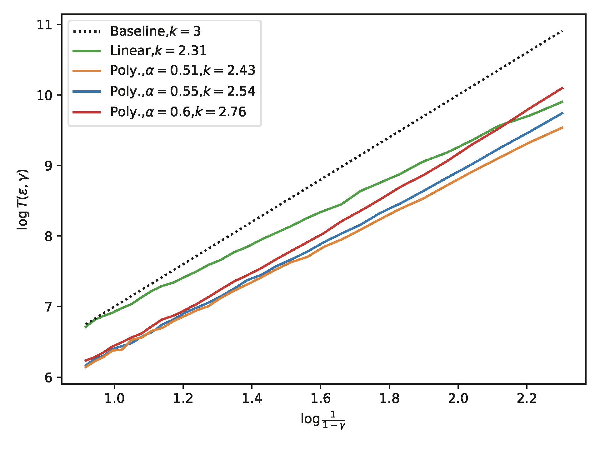
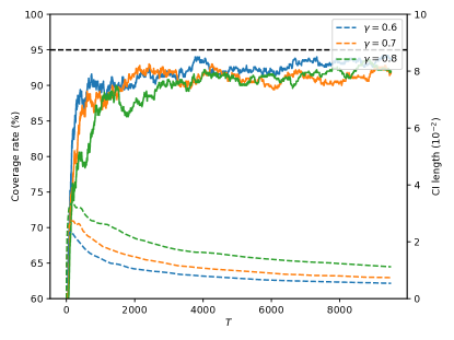
Figure 3: Left: log-log plots of the sample complexity $T(\varepsilon,\gamma)$ versus the discount complexity parameter $(1-\gamma)^{-1}$. Right: the coverage rate and the average length of the 95% confidence interval for regularized Q-Learning.

Appendix J DETAILS OF EXPERIMENTS

The setup of MDP.

According to Theorem 5.1, for sufficiently small error $\varepsilon>0$, we expect the sample complexity $T(\varepsilon,\gamma)$ is always upper bounded by $\|\mathrm{diag}(\mathrm{Var}_{\bm{Q}})\|_{\infty}$ and $\frac{1}{(1-\gamma)^{3}}$ at a worst case. To ensure Assumption 3.2, we consider a random MDP. In particular, for each $(s,a)$ pair, the random reward $R(s,a)\sim{\mathcal{U}}(0,1)$ is the uniformly sampled from $(0,1)$ and the transition probability $P(s^{\prime}|s,a)=u(s^{\prime})/\sum_{s}u(s)$, where $u(s)\overset{i.i.d.}{\sim}{\mathcal{U}}(0,1)$. The size of the MDP we choose is $|{\mathcal{S}}|=4$, $|{\mathcal{A}}|=3$. We consider 30 different values of $\gamma$ equispaced between $0.6$ and $0.9$. For a given $\gamma$, we run Q-learning algorithm for $10^{5}$ steps (which already ensures convergence) and repeat the process independently for $10^{3}$ times. Finally, we average the $\ell_{\infty}$ error $\|\bar{{\bm{Q}}}_{T}-{\bm{Q}}^{*}\|_{\infty}$ of the $10^{3}$ independent trials as an approximation of ${\mathbb{E}}\|\bar{{\bm{Q}}}_{T}-{\bm{Q}}^{*}\|_{\infty}$ and compute $T(\varepsilon,\gamma)$ by definition. The polynomial step size $\eta_{t}=t^{-\alpha}$ uses $\alpha\in\{0.51,0.55,0.60\}$ and the resacled linear step size is $\eta_{t}=(1+(1-\gamma)t)^{-1}$. In Figure 2, we choose $\varepsilon=e^{-4}$ and plot the results on a log-log scale. We then plot the least-squares fits through these points and the slopes of these lines are also provided in the legend.

Confirming the theoretical predictions.

In the body, we show the least-squares fits through the points $\{(\log\|\mathrm{diag}(\mathrm{Var}_{\bm{Q}})\|_{\infty},\log T(\varepsilon,\gamma))\}_{\gamma\in\Gamma}$. As a complementary, we also show the fits through $\{(\log(1-\gamma)^{-1},\log T(\varepsilon,\gamma))\}_{\gamma\in\Gamma}$ in Figure 3.

Online inference experiments.

We visualize the empirical coverage rate and confidence interval lengths of averaged Q-Learning in Figure 1. We use the random scaling method (Algorithm 1 in [Lee et al., 2021]) to compute the weighting matrix ${\bm{W}}_{T}\in{\mathbb{R}}^{D\times D}$ where ${\bm{W}}_{T}=\int_{0}^{1}\bar{{\bm{\phi}}}_{T}(r)\bar{{\bm{\phi}}}_{T}(r)^{\top}\mathrm{d}r$ and $\bar{{\bm{\phi}}}_{T}(r)={{\bm{\phi}}}_{T}(r)-r\cdot{{\bm{\phi}}}_{T}(1)$. We focus on the inference of the optimal value function on the first state $s_{0}$ and the first action $a_{0}$, i.e., $Q^{*}(s_{0},a_{0})$. We use $10^{4}$ steps of value iteration to compute the optimal value function ${\bm{Q}}^{*}$. From [Lee et al., 2021, Li et al., 2022], the asymptotic confidence interval is given by

$$\left[\bar{Q}_{T}(s_{0},a_{0})-6.753\sqrt{\frac{{\bm{W}}_{T}((s_{0},a_{0}),(s_{0},a_{0}))}{T}},\bar{Q}_{T}(s_{0},a_{0})+6.753\sqrt{\frac{{\bm{W}}_{T}((s_{0},a_{0}),(s_{0},a_{0}))}{T}}\right].$$

We set $T=10^{4}$ and discard the first $5\%$ samples as a warm-up. This warm-up is quite important; otherwise ${\bm{W}}_{T}$ would change rapidly (as a result of fast convergence of ${\bm{Q}}_{T}$) and deteriorate the performance. The performance is measured by two statistics: the coverage rate and the average length of the 95% confidence interval. We also provide similar results for regularized Q-Learning in Figure 3.

References

- Abadir and Paruolo [2002] Karim M Abadir and Paolo Paruolo. Simple robust testing of regression hypotheses: A comment. Econometrica, 70(5):2097–2099, 2002.
- Abounadi et al. [2002] Jinane Abounadi, Dimitri P Bertsekas, and Vivek Borkar. Stochastic approximation for nonexpansive maps: Application to Q-learning algorithms. SIAM Journal on Control and Optimization, 41(1):1–22, 2002.
- Agarwal et al. [2020] Alekh Agarwal, Sham Kakade, and Lin F Yang. Model-based reinforcement learning with a generative model is minimax optimal. In Conference on Learning Theory, pages 67–83. PMLR, 2020.
- Ahmed et al. [2019] Zafarali Ahmed, Nicolas Le Roux, Mohammad Norouzi, and Dale Schuurmans. Understanding the impact of entropy on policy optimization. In International Conference on Machine Learning, pages 151–160. PMLR, 2019.
- Anschel et al. [2017] Oron Anschel, Nir Baram, and Nahum Shimkin. Averaged-dqn: Variance reduction and stabilization for deep reinforcement learning. In International Conference on Machine Learning, pages 176–185. PMLR, 2017.
- Azar et al. [2013] Mohammad Gheshlaghi Azar, Rémi Munos, and Hilbert J Kappen. Minimax PAC bounds on the sample complexity of reinforcement learning with a generative model. Machine Learning, 91(3):325–349, 2013.
- Batir [2008] Necdet Batir. Inequalities for the gamma function. Archiv der Mathematik, 91(6):554–563, 2008.
- Beck and Srikant [2012] Carolyn L Beck and Rayadurgam Srikant. Error bounds for constant step-size Q-learning. Systems and Control Letters, 61(12):1203–1208, 2012.
- Bhandari et al. [2018] Jalaj Bhandari, Daniel Russo, and Raghav Singal. A finite time analysis of temporal difference learning with linear function approximation. In Conference on Learning Theory, pages 1691–1692. PMLR, 2018.
- Borkar et al. [2021] Vivek Borkar, Shuhang Chen, Adithya Devraj, Ioannis Kontoyiannis, and Sean Meyn. The ODE method for asymptotic statistics in stochastic approximation and reinforcement learning. arXiv preprint arXiv:2110.14427, 2021.
- Borkar [2009] Vivek S Borkar. Stochastic Approximation: A Dynamical Systems Viewpoint, volume 48. Springer, 2009.
- Borkar and Meyn [2000] Vivek S Borkar and Sean P Meyn. The ODE method for convergence of stochastic approximation and reinforcement learning. SIAM Journal on Control and Optimization, 38(2):447–469, 2000.
- Burkholder [1988] Donald L Burkholder. Sharp inequalities for martingales and stochastic integrals. Astérisque, 157(158):75–94, 1988.
- Cen et al. [2022] Shicong Cen, Chen Cheng, Yuxin Chen, Yuting Wei, and Yuejie Chi. Fast global convergence of natural policy gradient methods with entropy regularization. Operations Research, 70(4):2563–2578, 2022.
- Chen et al. [2020a] Xi Chen, Jason D Lee, Xin T Tong, and Yichen Zhang. Statistical inference for model parameters in stochastic gradient descent. Annals of Statistics, 48(1):251–273, 2020a.
- Chen et al. [2019] Zaiwei Chen, Sheng Zhang, Thinh T Doan, John-Paul Clarke, and Siva Theja Maguluri. Finite-sample analysis of nonlinear stochastic approximation with applications in reinforcement learning. arXiv preprint arXiv:1905.11425, 2019.
- Chen et al. [2020b] Zaiwei Chen, Siva Theja Maguluri, Sanjay Shakkottai, and Karthikeyan Shanmugam. Finite-sample analysis of stochastic approximation using smooth convex envelopes. arXiv e-prints, pages arXiv–2002, 2020b.
- Chen et al. [2021] Zaiwei Chen, Siva Theja Maguluri, Sanjay Shakkottai, and Karthikeyan Shanmugam. A Lyapunov theory for finite-sample guarantees of asynchronous Q-learning and TD-learning variants. arXiv preprint arXiv:2102.01567, 2021.
- Donsker [1951] Monroe David Donsker. An invariance principle for certain probability limit theorems. American Mathematical Society, pages 1–10, 1951.
- Dudley [2014] Richard M Dudley. Uniform Central Limit Theorems, volume 142. Cambridge University Press, 2014.
- Durmus et al. [2022] Alain Durmus, Eric Moulines, Alexey Naumov, and Sergey Samsonov. Finite-time high-probability bounds for Polyak-Ruppert averaged iterates of linear stochastic approximation. arXiv preprint arXiv:2207.04475, 2022.
- Even-Dar et al. [2003] Eyal Even-Dar, Yishay Mansour, and Peter Bartlett. Learning rates for Q-learning. Journal of Nachine Learning Research, 5(1), 2003.
- Eysenbach and Levine [2021] Benjamin Eysenbach and Sergey Levine. Maximum entropy RL (provably) solves some robust RL problems. In International Conference on Learning Representations, 2021.
- Fox et al. [2016] Roy Fox, Ari Pakman, and Naftali Tishby. Taming the noise in reinforcement learning via soft updates. In Conference on Uncertainty in Artificial Intelligence, pages 202–211, 2016.
- Freedman [1975] David A Freedman. On tail probabilities for martingales. Annals of Probability, pages 100–118, 1975.
- Gadat et al. [2018] Sébastien Gadat, Fabien Panloup, and Sofiane Saadane. Stochastic heavy ball. Electronic Journal of Statistics, 12(1):461–529, 2018.
- Gower et al. [2020] Robert M Gower, Mark Schmidt, Francis Bach, and Peter Richtárik. Variance-reduced methods for machine learning. Proceedings of the IEEE, 108(11):1968–1983, 2020.
- Hall and Heyde [2014] Peter Hall and Christopher C Heyde. Martingale Limit Theory and its Application. Academic Press, 2014.
- Hao et al. [2021] Botao Hao, Xiang Ji, Yaqi Duan, Hao Lu, Csaba Szepesvári, and Mengdi Wang. Bootstrapping statistical inference for off-policy evaluation. arXiv preprint arXiv:2102.03607, 2021.
- Jaakkola et al. [1993] Tommi Jaakkola, Michael I. Jordan, and Satinder P. Singh. Convergence of stochastic iterative dynamic programming algorithms. In Advances in Neural Information Processing Systems, 1993.
- Jacod and Shiryaev [2003] Jean Jacod and Albert N Shiryaev. Skorokhod topology and convergence of processes. In Limit Theorems for Stochastic Processes, pages 324–388. Springer, 2003.
- Jiang and Li [2016] Nan Jiang and Lihong Li. Doubly robust off-policy value evaluation for reinforcement learning. In International Conference on Machine Learning, pages 652–661. PMLR, 2016.
- Jirak [2017] Moritz Jirak. On weak invariance principles for partial sums. Journal of Theoretical Probability, 30(3):703–728, 2017.
- Kallus and Uehara [2020] Nathan Kallus and Masatoshi Uehara. Double reinforcement learning for efficient off-policy evaluation in Markov decision processes. J. Mach. Learn. Res., 21(167):1–63, 2020.
- Kearns and Singh [1999] Michael Kearns and Satinder Singh. Finite-sample convergence rates for Q-learning and indirect algorithms. Advances in Neural Information Processing Systems, pages 996–1002, 1999.
- Kearns et al. [2002] Michael Kearns, Yishay Mansour, and Andrew Y Ng. A sparse sampling algorithm for near-optimal planning in large Markov decision processes. Machine Learning, 49(2):193–208, 2002.
- Khamaru et al. [2021a] Koulik Khamaru, Ashwin Pananjady, Feng Ruan, Martin J Wainwright, and Michael I Jordan. Is temporal difference learning optimal? An instance-dependent analysis. SIAM Journal on Mathematics of Data Science, 3(4):1013–1040, 2021a.
- Khamaru et al. [2021b] Koulik Khamaru, Eric Xia, Martin J Wainwright, and Michael I Jordan. Instance-optimality in optimal value estimation: Adaptivity via variance-reduced Q-learning. arXiv preprint arXiv:2106.14352, 2021b.
- Khamaru et al. [2022] Koulik Khamaru, Eric Xia, Martin J Wainwright, and Michael I Jordan. Instance-dependent confidence and early stopping for reinforcement learning. arXiv preprint arXiv:2201.08536, 2022.
- Kiefer et al. [2000] Nicholas M Kiefer, Timothy J Vogelsang, and Helle Bunzel. Simple robust testing of regression hypotheses. Econometrica, 68(3):695–714, 2000.
- Konda and Tsitsiklis [1999] Vijaymohan Konda and John Tsitsiklis. Actor-critic algorithms. Advances in Neural Information Processing Systems, 12, 1999.
- Kozuno et al. [2022] Tadashi Kozuno, Wenhao Yang, Nino Vieillard, Toshinori Kitamura, Yunhao Tang, Jincheng Mei, Pierre Ménard, Mohammad Gheshlaghi Azar, Michal Valko, Rémi Munos, et al. KL-entropy-regularized RL with a generative model is minimax optimal. arXiv preprint arXiv:2205.14211, 2022.
- Kushner and Yin [2003] Harold Kushner and G George Yin. Stochastic Approximation and Recursive Algorithms and Applications, volume 35. Springer Science & Business Media, 2003.
- Lattimore and Hutter [2014] Tor Lattimore and Marcus Hutter. Near-optimal PAC bounds for discounted MDPs. Theoretical Computer Science, 558:125–143, 2014.
- Lee and He [2019a] Donghwan Lee and Niao He. Target-based temporal-difference learning. In International Conference on Machine Learning, pages 3713–3722. PMLR, 2019a.
- Lee and He [2019b] Donghwan Lee and Niao He. A unified switching system perspective and ODE analysis of Q-learning algorithms. arXiv preprint arXiv:1912.02270, 2019b.
- Lee et al. [2021] Sokbae Lee, Yuan Liao, Myung Hwan Seo, and Youngki Shin. Fast and robust online inference with stochastic gradient descent via random scaling. arXiv preprint arXiv:2106.03156, 2021.
- Lehmann and Casella [2006] Erich L Lehmann and George Casella. Theory of Point Estimation. Springer Science & Business Media, 2006.
- Li et al. [2020a] Gen Li, Yuting Wei, Yuejie Chi, Yuantao Gu, and Yuxin Chen. Breaking the sample size barrier in model-based reinforcement learning with a generative model. Advances in Neural Information Processing Systems, 33:12861–12872, 2020a.
- Li et al. [2020b] Gen Li, Yuting Wei, Yuejie Chi, Yuantao Gu, and Yuxin Chen. Sample complexity of asynchronous Q-learning: Sharper analysis and variance reduction. arXiv preprint arXiv:2006.03041, 2020b.
- Li et al. [2021a] Gen Li, Changxiao Cai, Yuxin Chen, Yuantao Gu, Yuting Wei, and Yuejie Chi. Is Q-learning minimax optimal? A tight sample complexity analysis. arXiv preprint arXiv:2102.06548, 2021a.
- Li et al. [2021b] Tianjiao Li, Guanghui Lan, and Ashwin Pananjady. Accelerated and instance-optimal policy evaluation with linear function approximation. arXiv preprint arXiv:2112.13109, 2021b.
- Li et al. [2022] Xiang Li, Jiadong Liang, Xiangyu Chang, and Zhihua Zhang. Statistical estimation and online inference via local SGD. Proceedings of Thirty Fifth Conference on Learning Theory, 178:1613–1661, 2022.
- Lillicrap et al. [2016] Timothy P Lillicrap, Jonathan J Hunt, Alexander Pritzel, Nicolas Heess, Tom Erez, Yuval Tassa, David Silver, and Daan Wierstra. Continuous control with deep reinforcement learning. In International Conference on Learning of Representations, 2016.
- Luckett et al. [2019] Daniel J Luckett, Eric B Laber, Anna R Kahkoska, David M Maahs, Elizabeth Mayer-Davis, and Michael R Kosorok. Estimating dynamic treatment regimes in mobile health using V-learning. Journal of the American Statistical Association, 2019.
- Melo et al. [2008] Francisco S Melo, Sean P Meyn, and M Isabel Ribeiro. An analysis of reinforcement learning with function approximation. In International Conference on Machine Learning, pages 664–671, 2008.
- Mokkadem and Pelletier [2006] Abdelkader Mokkadem and Mariane Pelletier. Convergence rate and averaging of nonlinear two-time-scale stochastic approximation algorithms. The Annals of Applied Probability, 16(3):1671–1702, 2006.
- Moore Jr [2010] Terrence Joseph Moore Jr. A theory of Cramér-Rao bounds for constrained parametric models. University of Maryland, College Park, 2010.
- Mou et al. [2020a] Wenlong Mou, Chris Junchi Li, Martin J Wainwright, Peter L Bartlett, and Michael I Jordan. On linear stochastic approximation: Fine-grained Polyak-Ruppert and non-asymptotic concentration. In Conference on Learning Theory, pages 2947–2997. PMLR, 2020a.
- Mou et al. [2020b] Wenlong Mou, Ashwin Pananjady, and Martin J Wainwright. Optimal oracle inequalities for solving projected fixed-point equations. arXiv preprint arXiv:2012.05299, 2020b.
- Moulines and Bach [2011] Eric Moulines and Francis Bach. Non-asymptotic analysis of stochastic approximation algorithms for machine learning. Advances in Neural Information Processing Systems, 24:451–459, 2011.
- Newey [1990] Whitney K Newey. Semiparametric efficiency bounds. Journal of Applied Econometrics, 5(2):99–135, 1990.
- Pananjady and Wainwright [2020] Ashwin Pananjady and Martin J Wainwright. Instance-dependent bounds for policy evaluation in tabular reinforcement learning. IEEE Transactions on Information Theory, 67(1):566–585, 2020.
- Polyak and Juditsky [1992] Boris T Polyak and Anatoli B Juditsky. Acceleration of stochastic approximation by averaging. SIAM Journal on Control and Optimization, 30(4):838–855, 1992.
- Puterman and Brumelle [1979] Martin L Puterman and Shelby L Brumelle. On the convergence of policy iteration in stationary dynamic programming. Mathematics of Operations Research, 4(1):60–69, 1979.
- Qu and Wierman [2020] Guannan Qu and Adam Wierman. Finite-time analysis of asynchronous stochastic approximation and Q-learning. In Conference on Learning Theory, pages 3185–3205. PMLR, 2020.
- Robbins and Monro [1951] Herbert Robbins and Sutton Monro. A stochastic approximation method. The Annals of Mathematical Statistics, pages 400–407, 1951.
- Ruppert [1988] David Ruppert. Efficient estimations from a slowly convergent Robbins-Monro process. Technical report, Cornell University Operations Research and Industrial Engineering, 1988.
- Shah and Xie [2018] Devavrat Shah and Qiaomin Xie. Q-learning with nearest neighbors. In Advances in Neural Information Processing Systems, pages 3115–3125, 2018.
- Shi et al. [2020] Chengchun Shi, Sheng Zhang, Wenbin Lu, and Rui Song. Statistical inference of the value function for reinforcement learning in infinite horizon settings. arXiv preprint arXiv:2001.04515, 2020.
- Sidford et al. [2018a] Aaron Sidford, Mengdi Wang, Xian Wu, Lin F Yang, and Yinyu Ye. Near-optimal time and sample complexities for solving Markov decision processes with a generative model. In Advances in Neural Information Processing Systems, pages 5192–5202, 2018a.
- Sidford et al. [2018b] Aaron Sidford, Mengdi Wang, Xian Wu, and Yinyu Ye. Variance reduced value iteration and faster algorithms for solving Markov decision processes. In Proceedings of the Twenty-Ninth Annual ACM-SIAM Symposium on Discrete Algorithms, pages 770–787. SIAM, 2018b.
- Su and Zhu [2018] Weijie J Su and Yuancheng Zhu. Uncertainty quantification for online learning and stochastic approximation via hierarchical incremental gradient descent. arXiv preprint arXiv:1802.04876, 2018.
- Sutton and Barto [2018] Richard S Sutton and Andrew G Barto. Reinforcement Learning: An Introduction. MIT Press, 2018.
- Szepesvári et al. [1998] Csaba Szepesvári et al. The asymptotic convergence-rate of Q-learning. Advances in Neural Information Processing Systems, pages 1064–1070, 1998.
- Tsiatis [2006] Anastasios A Tsiatis. Semiparametric Theory and Missing Data. Springer, 2006.
- Tsitsiklis [1994] John N Tsitsiklis. Asynchronous stochastic approximation and Q-learning. Machine Learning, 16(3):185–202, 1994.
- Uehara et al. [2020] Masatoshi Uehara, Jiawei Huang, and Nan Jiang. Minimax weight and Q-function learning for off-policy evaluation. In International Conference on Machine Learning, pages 9659–9668. PMLR, 2020.
- Van der Vaart [2000] Aad W Van der Vaart. Asymptotic Statistics. Cambridge University Press, 2000.
- Vermeulen [2011] Karel Vermeulen. Semiparametric Efficiency. Gent Universiteit, 2011.
- Wainwright [2019a] Martin J Wainwright. High-Dimensional Statistics: A Non-Asymptotic Viewpoint. Cambridge University Press, 2019a.
- Wainwright [2019b] Martin J Wainwright. Stochastic approximation with cone-contractive operators: Sharp -bounds for Q-learning. arXiv preprint arXiv:1905.06265, 2019b.
- Wainwright [2019c] Martin J Wainwright. Variance-reduced Q-learning is minimax optimal. arXiv preprint arXiv:1906.04697, 2019c.
- Watkins [1989] Christopher Watkins. Learning from delayed rewards. PhD thesis, 1989.
- Yang et al. [2019] Wenhao Yang, Xiang Li, and Zhihua Zhang. A regularized approach to sparse optimal policy in reinforcement learning. In Advances in Neural Information Processing Systems, pages 5938–5948, 2019.
- Yang et al. [2021] Wenhao Yang, Liangyu Zhang, and Zhihua Zhang. Towards theoretical understandings of robust Markov decision processes: Sample complexity and asymptotics. arXiv preprint arXiv:2105.03863, 2021.
- Yin and Wang [2020] Ming Yin and Yu-Xiang Wang. Asymptotically efficient off-policy evaluation for tabular reinforcement learning. In International Conference on Artificial Intelligence and Statistics, pages 3948–3958. PMLR, 2020.
- Yin and Wang [2021] Ming Yin and Yu-Xiang Wang. Towards instance-optimal offline reinforcement learning with pessimism. Advances in Neural Information Processing Systems, 34, 2021.
- Zhu et al. [2021] Wanrong Zhu, Xi Chen, and Wei Biao Wu. Online covariance matrix estimation in stochastic gradient descent. Journal of the American Statistical Association, pages 1–30, 2021.