Frequency-Aware Contrastive Learning for Neural Machine Translation

Abstract

Low-frequency word prediction remains a challenge in modern neural machine translation (NMT) systems. Recent adaptive training methods promote the output of infrequent words by emphasizing their weights in the overall training objectives. Despite the improved recall of low-frequency words, their prediction precision is unexpectedly hindered by the adaptive objectives. Inspired by the observation that low-frequency words form a more compact embedding space, we tackle this challenge from a representation learning perspective. Specifically, we propose a frequency-aware token-level contrastive learning method, in which the hidden state of each decoding step is pushed away from the counterparts of other target words, in a soft contrastive way based on the corresponding word frequencies. We conduct experiments on widely used NIST Chinese-English and WMT14 English-German translation tasks. Empirical results show that our proposed methods can not only significantly improve the translation quality but also enhance lexical diversity and optimize word representation space. Further investigation reveals that, comparing with related adaptive training strategies, the superiority of our method on low-frequency word prediction lies in the robustness of token-level recall across different frequencies without sacrificing precision.

1 Introduction

Neural Machine Translation (NMT, Sutskever, Vinyals, and Le 2014; Bahdanau, Cho, and Bengio 2015; Vaswani et al. 2017) has made revolutionary advances in the past several years. However, the effectiveness of these data-driven NMT systems is heavily reliant on the large-scale training corpus, where the word frequencies demonstrate a long-tailed distribution according to Zipf’s Law (Zipf 1949). The inherently imbalanced data leads NMT models to commonly prioritize the generation of frequent words while neglect the rare ones. Therefore, predicting low-frequency yet semantically rich words remains a bottleneck of current data-driven NMT systems (Vanmassenhove, Shterionov, and Way 2019).

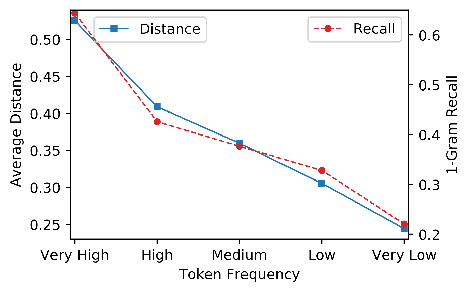
Figure 1: Average token representation distance and 1-gram recall of token buckets with different frequencies on NIST Zh-en test sets and a well-trained vanilla Transformer model. We sort all tokens in target vocabulary based on their frequencies in LDC training set, and divide them into five equal-size buckets. Obviously, the average token distance and 1-gram recall similarly deteriorate with decreasing frequency.

A common practice to facilitate the generation of infrequent words is to smooth the frequency distribution of tokens. For example, it has become a de-facto standard to split words into more fine-grained translation units such as subwords (Wu et al. 2016; Sennrich, Haddow, and Birch 2016). Despite that, NMT systems still face the token imbalance phenomenon (Gu et al. 2020). More recently, some efforts have been dedicated to applying adaptive weights to target tokens in training objectives based on their frequency (Gu et al. 2020; Xu et al. 2021b). By heightening the exposure of low-frequency tokens during training, these models can meliorate the neglect of low-frequency tokens and improve lexical diversity of the translations. However, simply promoting low-frequency tokens via loss re-weighting may potentially sacrifice the learning of high-frequency ones  (Gu et al. 2020; Wan et al. 2020; Zhou et al. 2020). Besides, our further investigation on these methods reveals that generating more unusual tokens comes at the unexpected expense of their prediction precision (Section 5.4).

In modern NMT models, the categorical distribution of the predicted word in a decoding step is generated by multiplying the last-layer hidden state by the softmax embedding matrix. Therefore, unlike previous explorations, we preliminarily investigate low-frequency word predictions from the perspective of the word representation. As illustrate in Figure 1, we divide all the target tokens into several subsets according to their frequencies, and check token-level predictions of each subset based on the vanilla Transformer (Vaswani et al. 2017). Our observation is that the average word embedding distance and 1-gram recall of these subsets demonstrate a similar downward trend with word frequency decrease.

Another important fact is that the embedding of a ground-truth word and the corresponding hidden state will be pushed together during training to get a more significant likelihood (Gao et al. 2019). It inspires us that making the hidden states more diversified could potentially benefit the prediction of low-frequency words. On the one hand, more diversified hidden states could expand word embedding space due to their collaboration in NMT models, which is exactly what we expect given the correlation shown in Figure 1. On the other hand, regarding each decoding step as a multi-class classification task, more diversified hidden states can generate better classification boundaries that are more friendly to long-tailed classes (or low-frequency words).

To this end, we propose incorporating contrastive learning into NMT models to improve low-frequency word predictions. Our contrastive learning mechanism has two main characteristics. Firstly, unlike previous efforts that contrast at the sentence level (Pan et al. 2021; Lee, Lee, and Hwang 2021), we exploit token-level contrast at each decoding step to produce hidden states more uniformly distributed. Secondly, our contrastive learning is frequency-aware. As long-tailed tokens form a more compact embedding space, we propose to amplify the contrastive effect for relatively low-frequency tokens. In particular, for an anchor and one of its negatives, we will apply a soft weight to the corresponding distances based on their frequencies—generally, the lower their frequency, the greater the weight.

We have conducted experiments on Chinese-English and English-German translation tasks. The experimental results demonstrate that our method can significantly outperform the baselines and consistently improve the translation of words with different frequencies, especially rare ones.

Overall, our contributions are mainly three-fold:

• We propose a novel Frequency-aware token-level Contrastive Learning method (FCL) for NMT, providing a new insight of addressing the low-frequency word prediction from the representation learning perspective.

• Extensive experiments on Zh-En and En-De translation tasks show that FCL remarkably boosts translation performance, enriches lexical diversity, and improves word representation space.

• Compared with previous adaptive training methods, FCL demonstrates the superiority of (1) promoting the output of low-frequency words without sacrificing the token-level prediction precision and (2) consistently improving token-level predictions across different frequencies, especially for infrequent words.

2 Related Work

Low-Frequency Word Translation

is a persisting challenge for NMT due to the token imbalance phenomenon. Conventional researches range from introducing fine-grained translation units (Luong and Manning 2016; Lee, Cho, and Hofmann 2017), seeking optimal vocabulary (Wu et al. 2016; Sennrich, Haddow, and Birch 2016; Gowda and May 2020; Liu et al. 2021), to incorporating external lexical knowledge (Luong et al. 2015; Arthur, Neubig, and Nakamura 2016; Zhang et al. 2021). Recently, some approaches alleviate this problem by well-designed loss function with adaptive weights, in light of the token frequency (Gu et al. 2020) or bilingual mutual information (Xu et al. 2021b). Inspired by these work, we instead proposed a token-level contrastive learning method and introduce frequency-aware soft weights to adaptively contrast the representations of target words.

Contrastive Learning

has been a widely-used technique to learn representations in both computer vision (Hjelm et al. 2019; Khosla et al. 2020; Chen et al. 2020) and neural language processing (Logeswaran and Lee 2018; Fang et al. 2020; Gao, Yao, and Chen 2021; Lin et al. 2021). There are also several recent literatures that attempt to boost machine translation with the effectiveness of contrastive learning. Yang et al. (2019) proposes to reduce word omission by max-margin loss. Pan et al. (2021) learns a universal cross-language representation with a contrastive learning paradigm for multilingual NMT. Lee, Lee, and Hwang (2021) adopt a contrastive learning method with perturbed examples to mitigates the exposure bias problem. Different from the previous work that contrasts the sentence-level log-likelihoods or representations, our contrastive learning methods pay attention to token-level representations and introduce frequency feature to facilitate rare word generation.

Representation Degeneration

has attracted increasing interest recently (Gao et al. 2019; Xu et al. 2021a), which refers that the embedding space learned in language modeling or neural machine translation is squeezed into a narrow cone due to the weight tying trick. Recent researches mitigate this issue by performing regularization during training (Gao et al. 2019; Wang et al. 2020). The distinction between our methods and these work is that our contrastive methods are applied on the hidden representations of the diverse instances in the training corpus rather than directly performing regularizations on the softmax embeddings.

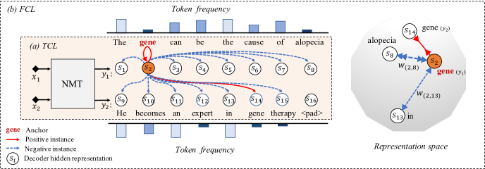
Figure 2: An example of Token-level Contrastive Learning (TCL) and Frequency-aware Contrastive Learning (FCL). (a) TCL contrasts the token-level hidden representations $s_{i}$ of the in-batch target tokens. For the anchor “gene” in the first sentence $y_{1}$, there are two sources for its positives, i.e., its counterpart with dropout noise (denoted by the red self-pointing arrow) and the “gene” in $y_{2}$. All other in-batch tokens serve as the negatives. (b) FCL further leverages token frequency information to apply frequency-aware soft weights $w(i,j)$ in contrasts. Thus the contrastive effect between relatively infrequent tokens (e.g., “gene” and “alopecia”) is amplified and they can be further pulled apart in the representation space.

3 Methodology

In this section, we mathematically describe the proposed Frequency-aware Contrastive Learning (FCL) method in detail. FCL firstly cast autoregressive neural machine translation as a sequence of classification tasks, and differentiate the hidden representations of different target tokens in Transformer decoder by a token-level contrastive learning method (TCL). To facilitate the translation of low-frequency words, we further equip TCL with frequency-aware soft weights, highlighting the classification boundary for the infrequent tokens. An overview of TCL and FCL is illustrated in Figure 2.

3.1 Token-Level Contrastive Learning

In this section we briefly introduce the Token-level Contrastive Learning (TCL) method for NMT. Different from the previous explorations in NMT which contrast the sentence-level representation in the scenario of multilingualism (Pan et al. 2021) or adding perturbation (Lee, Lee, and Hwang 2021), TCL exploits contrastive learning objectives in the token granularity. Concretely, TCL contrasts the hidden representations of target tokens before softmax classifier. There are two ways in TCL to construct positive instances for each target token: a supervised way to explore the presence of golden label in reference and a supplementary way to take advantage of dropout noise.

Supervised Contrastive Learning

For supervised contrastive learning, the underlying thought is to pulling together the same tokens and pushing apart the different tokens. Inspired by Khosla et al. (2020), we propose a token-level contrastive framework for NMT, which contrasts the in-batch token representations in Transformer decoder. For each target token, we explore the inherent supervised information in the reference to construct the positive samples by the same tokens from the minibatch, and the negative samples are formed by the in-batch tokens different from the anchor. In this way, the model can learn effective representation with clear boundaries for the target tokens.

Supplementary Positives with Dropout Noise

In a supervised contrast learning scenario, however, a target token may have no same token in the minibatch due to the token imbalance phenomenon. This limitation is particularly severe when it comes to low-frequency tokens. Thus the supervised contrastive objectives can barely ameliorate the representations of infrequent tokens since in most cases they have no positive instance. Inspired by Gao, Yao, and Chen (2021), we construct a pseudo positive instance for each anchor by applying independently sampled dropout strategy. By feeding a parallel sentence pair twice into the NMT model and applying different dropout samples, we can obtain a supplementary hidden representation for each target token with dropout noise. In this way, the supplement can serve as the positive instance for the original token representation. Thereby each target token will be assigned at least one positive instance for an effective contrastive learning.

Formalization

The proposed token-level contrastive leaning combines the above two strategies to build the positive instances and use the other in-batch tokens as the negatives. Formally, given a minibatch with $K$ parallel sentence pairs, $\{{\mathbf{x}}_{k},{\mathbf{y}}_{k}\}_{k=1...K}$, which contains a total of $M$ source tokens and $N$ target tokens, the translation probability $p(y_{i}|\mathbf{y}_{<i},\mathbf{x})$ for the $i^{th}$ in-batch target token $y_{i}$ is commonly calculated by multiplying the last-layer decoder hidden state $s_{i}$ by the softmax embedding matrix $\mathbf{W_{s}}$ in a softmax layer:

$$p(y_{i}|\mathbf{y}_{<i},\mathbf{x})\propto{\rm{exp}}(\mathbf{W_{s}}\cdot s_{i}),$$ (1)

In TCL, we feed the inputs to the model twice with independent dropout sample and get two hidden representations $s_{i}$ and $s^{\prime}_{i}$ for a target token $y_{i}$. For an anchor $s_{i}$, $s^{\prime}_{i}$ serves as the positive, as well as the representations of target tokens that same as $y_{i}$. The token-level contrastive objective can be formulated as:

$$L_{TCL}=-\frac{1}{N}\sum_{i=1}^{N}\sum_{s_{p}\in S_{p}(i)}{\rm log}\frac{e^{sim(s_{i}\cdot s_{p})}}{{\textstyle\sum_{j=1}^{N}}e^{sim(s_{i}\cdot s_{j})}},$$ (2)

where $sim(s_{i}\cdot s_{p})$ denotes the cosine similarity between $s_{i}$ and $s_{p}$. Here, $S_{p}(i)=S_{sup}(i)\cup S_{drop}(i)$ is the set of all positive instances for $y_{i}$. $S_{sup}(i)=\{s_{p}:p\neq i,p=1...N,y_{p}=y_{i}\}$ denotes the positives in supervised contrastive setting, and $S_{drop}(i)=\{s^{\prime}_{i}\}$ is the counterpart constructed by dropout noise.

Finally, the overall training objective combines the traditional NMT objective $L_{MT}$ and the token-level contrastive objective $L_{TCL}$:

$$L=L_{MT}+\lambda L_{TCL},$$ (3)

where $\lambda$ is a hyperparameter to balance the effect of TCL.

3.2 Frequency-Aware Contrastive Learning

Token-level contrastive learning treats tokens equally when widening their boundary. However, due to the severe imbalance on token frequency, a small number of high-frequency tokens make up the majority of token occurrence in a minibatch while most low-frequency words rarely occur in a minibatch. Thus, TCL mainly contrasts the frequent tokens whereas neglects the contrast between the low-frequency tokens. In fact, as illustrated in Section 1, the representation of infrequent tokens are more compact and underinformative, which are in more need of amelioration. Intuitively, in this scenario a better blueprint for contrast is to put more emphasis on the contrast of infrequent tokens. As a consequence, the model can assign more distinctive representations for infrequent tokens and facilitate the translation of infrequent tokens. To this end, we further propose a Frequency-aware Contrast Learning (FCL) method, which utilizes a soft contrastive paradigm to assign frequency-aware soft weights in contrast and thus highlights the contrast of the infrequent tokens. Formally, for each target token $y_{i}$, we assign a soft weight $w(i,j)$ for the contrast between the anchor $y_{i}$ and a negative sample $y_{j}$. This frequency-aware is determined by the frequencies of both $y_{i}$ and $y_{j}$. In FCL, the positives and negatives are built up with the same strategy in token-level contrastive learning. The soft contrastive learning objects can be rewritten as follows:

$$L_{FCL}=-\frac{1}{N}\sum_{i=1}^{N}\sum_{s_{p}\in S_{p}(i)}{\rm log}\frac{e^{sim(s_{i}\cdot s_{p})}}{{\textstyle\sum_{j=1}^{N}}w(i,j)e^{sim(s_{i}\cdot s_{j})}},$$ (4)

where $w(i,j)$ is a soft weight in light of frequencies of both the anchor $y_{i}$ and a negative sample $y_{j}$. The underlying insight is to highlight the contrastive effect for infrequent tokens. The frequency-aware soft weight $w(i,j)$ is formulated as:

$$w(i,j)={\gamma}f(y_{i})f(y_{j}),$$ (5)

$$f(y {}_{i})=1-\frac{{\rm log(Count}(y_{i}))}{\underset{j=1...N}{\rm max}{\rm log(Count}(y_{j}))},$$

where $f(y_{i})$ and $f(y_{j})$ are the individual frequency score for $y_{i}$ and $y_{j}$, respectively. $\gamma$ is a scale factor for $w(i,j)$. Count$(y_{i})$ denotes the word count of $y_{i}$ in the training set. In our implement, the mean value of frequency-aware weights for all negatives of anchor $y_{i}$ is normalized to be 1.

Accordingly, we weight the traditional NMT objective $L_{MT}$ and the frequency-aware contrastive objective $L_{FCL}$ by a hyperparameter $\lambda$ as follows:

$$L=L_{MT}+\lambda L_{FCL}.$$ (6)

4 Experimental Settings

	Zh-En							En-De
Systems	MT02	MT03	MT04	MT05	MT08	AVG	$\Delta$	WMT14	$\Delta$
Baseline NMT systems
Transformer	47.06	46.89	47.63	45.40	35.02	44.40		27.84
Focal	47.11	45.70	47.32	45.26	35.61	44.20	-0.20	27.91	+0.07
Linear	46.84	46.27	47.26	45.62	35.59	44.32	-0.08	28.02	+0.18
Exponential	46.93	47.45	47.52	46.11	36.04	44.81	+0.41	28.17	+0.33
Chi-Square	47.14	47.15	47.68	45.46	36.15	44.72	+0.32	28.31	+0.47
BMI	48.05	47.11	47.64	45.97	35.93	44.94	+0.54	28.28	+0.44
CosReg	47.11	46.98	47.72	46.60	36.66	45.01	+0.61	28.38	+0.54
Our NMT systems
TCL	48.28††	47.90††	48.31††	46.23†	36.67††	45.48††	+1.08	28.51†	+0.67
FCL	48.95††	48.63††	48.38††	46.82††	37.00††	45.96††	+1.56	28.65††	+0.81

Table 1: Main results on NIST Zh-En and WMT14 En-De tasks. $\Delta$ shows the average BLEU improvements over the test sets compared with Transformer baseline. “$\dagger$” and “$\dagger\dagger$” indicate the improvement over Transformer is statistically significant ($p<$ 0.05 and $p<$ 0.01, respectively), estimated by bootstrap sampling (Koehn 2004).

4.1 Setup

Data Setting

We evaluate our model on both widely used NIST Chinese-to-Engish (Zh-En) and WMT14 English-German (En-De) translation tasks.

• For Zh-En translation, we use the LDC corpus as the training set, which consists of 1.25M sentence pairs. We adopt NIST 2006 (MT06) as the validation set and NIST 2002, 2003, 2004, 2005, 2008 datasets as the test sets.

• For En-De Translation, the training data contains 4.5M sentence pairs collected from WMT 2014 En-De dataset. We adapt newstest2013 as the validation set and test our model on newstest2014.

We adopt Moses tokenizer to deal with English and German sentences, and segment the Chinese sentences with the Stanford Segmentor. Following common practices, we employ byte pair encoding (Sennrich, Haddow, and Birch 2016) with 32K merge operations.

Implementation Details

We examine our model based on the advanced Transformer architecture and base setting (Vaswani et al. 2017). All the baseline systems and our models are implemented on top of THUMT toolkit (Zhang et al. 2017). During training, the dropout rate and label smoothing are set to 0.1. We employ the Adam optimizer with $\beta_{2}$ = 0.998. We use 1 GPU for the NIST Zh-En task and 4 GPUs for WMT14 En-De task. The batch size is 4096 for each GPU. The other hyper-parameters are the same as the default “base” configuration in Vaswani et al. (2017). The training of each model is early-stopped to maximize BLEU score on the development set. The best single model in validation is used for testing. We use $multi{\rm{-}}bleu.perl$ to calculate the case-sensitive BLEU score.

For TCL and FCL, the optimal $\lambda$ for contrastive learning loss is 2.0. The scale factor $\gamma$ in FCL is set to be 1.4. All these hyper-parameters are tuned on the validation set.

Note that compared with Transformer, TCL and FCL have no extra parameters and require no extra training data, hence demonstrating consistent inference efficiency. Due to the supplementary positives with dropout noise in contrastive objectives, the training speed of FCL is about 1.59$\times$ slower than vanilla Transformer.

4.2 Baselines

We re-implement and compare our proposed token-level contrastive learning (TCL) and frequency-aware contrastive learning (FCL) methods with the following baselines:

• Transformer (Vaswani et al. 2017) is the most widely-used NMT system with self-attention mechanism.

• Focal (Lin et al. 2017) is a classic adaptive training method proposed for tackling label imbalance problem in object detection. In Focal loss, difficult tokens with low prediction probabilities are assigned with higher learning rates. We treat it as a baseline because the low-frequency tokens are intuitively difficult to predict.

• Linear (Jiang et al. 2019) is an adaptive training method with a linear weight function of word frequency.

• Exponential (Gu et al. 2020) is an adaptive training method with the exponential weight function.

• Chi-Square (Gu et al. 2020) is an adaptive training method that adopts a chi-square distribution as the weight function. The exponential and chi-square weight functions are shown in Figure 3(d).

• BMI (Xu et al. 2021b) is a bilingual mutual information based adaptive training objective which estimates the learning difficulty between the source and the target to build the adaptive weighting function.

• CosReg (Gao et al. 2019) is a cosine regularization term to maximize the distance between any two word embeddings to mitigate representation degeneration problem. We also treat it as a baseline.

5 Experimental Results

5.1 Main Results

Table 1 shows the performance of the baseline models and our method variants on NIST Zh-En and WMT En-De translation tasks. We have the following observations.

First, regarding the adaptive training methods, those carefully designed adaptive objectives (e.g., Exponential, Chi-Square, and BMI) achieve slight performance improvement compared with two previous ones (Focal and Linear). As revealed in  Gu et al. (2020), Focal and Linear will harm high-frequency token prediction by simply highlighting the loss of low-frequency ones. In fact, our further investigation shows that these newly proposed adaptive objectives alleviate but do not eliminate the negative impact on more frequent tokens, and the increasing weight comes with an unexpected sacrifice in word prediction precision. This is the main reason for their marginal improvements (see more details in Section 5.4).

Second, even as a suboptimal model, our proposed TCL outperforms all adaptive training methods on both Zh-En and En-De translation tasks. This verifies that expanding softmax embedding latent space can effectively improve the translation quality, which is confirmed again by the results of CosReg. Compared with CosReg improving the uniformity using a data-independent regularizer, ours leverage the rich semantic information contained in the training instances to learn superior representations, thus performing a greater improvement.

Third, FCL further improves TCL, achieving the best performance and significantly outperform Transformer baseline on NIST Zh-En and WMT En-De tasks. For example, FCL achieves an impressive BLEU improvement of 1.56 over vanilla Transfomer on Zh-En translation. The results clearly demonstrate the merits of incorporating frequency-aware soft weights into contrasting.

Method	High	Medium	Low
Transformer	50.11	43.92	39.30
Exponential	49.89(-0.22)	44.20(+0.28)	40.42(+1.12)
Chi-Square	50.13(+0.02)	44.18(+0.26)	39.95(+0.65)
BMI	50.35(+0.24)	44.02(+0.10)	40.44(+1.14)
TCL	50.74(+0.63)	45.05(+1.13)	40.73(+1.43)
FCL	50.95(+0.84)	45.42(+1.50)	41.30(+2.00)

Table 2: BLEU scores on NIST Zh-En test subsets with different proportions of low-frequency words. “Low” denotes the subset in which the target sentences contain more low-frequency words, while “High” is the opposite. Our methods yield better translation quality across different subsets.

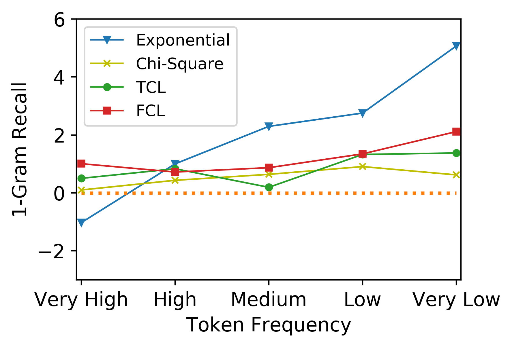
(a) 1-Gram Recall Gap

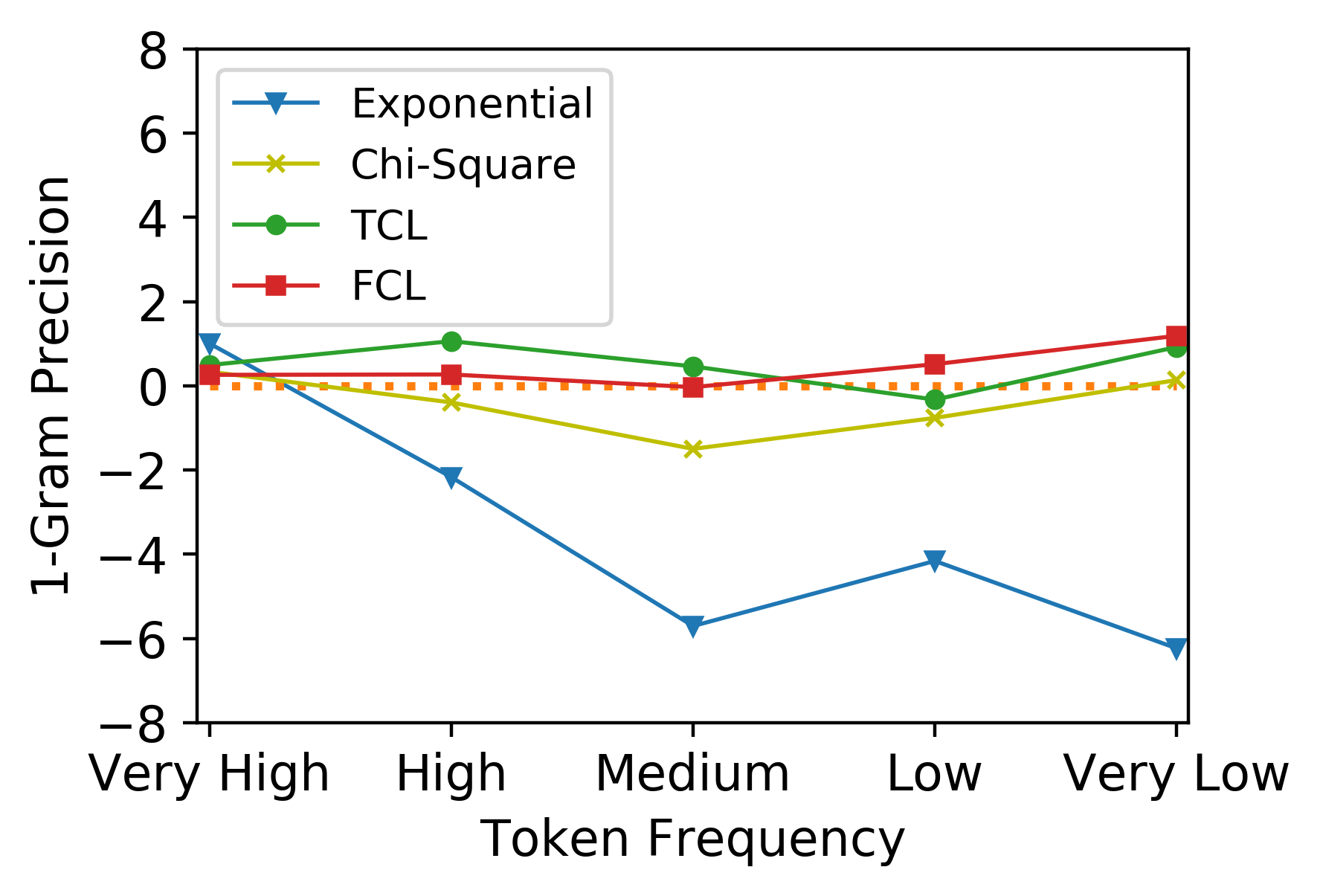
(b) 1-Gram Precision Gap

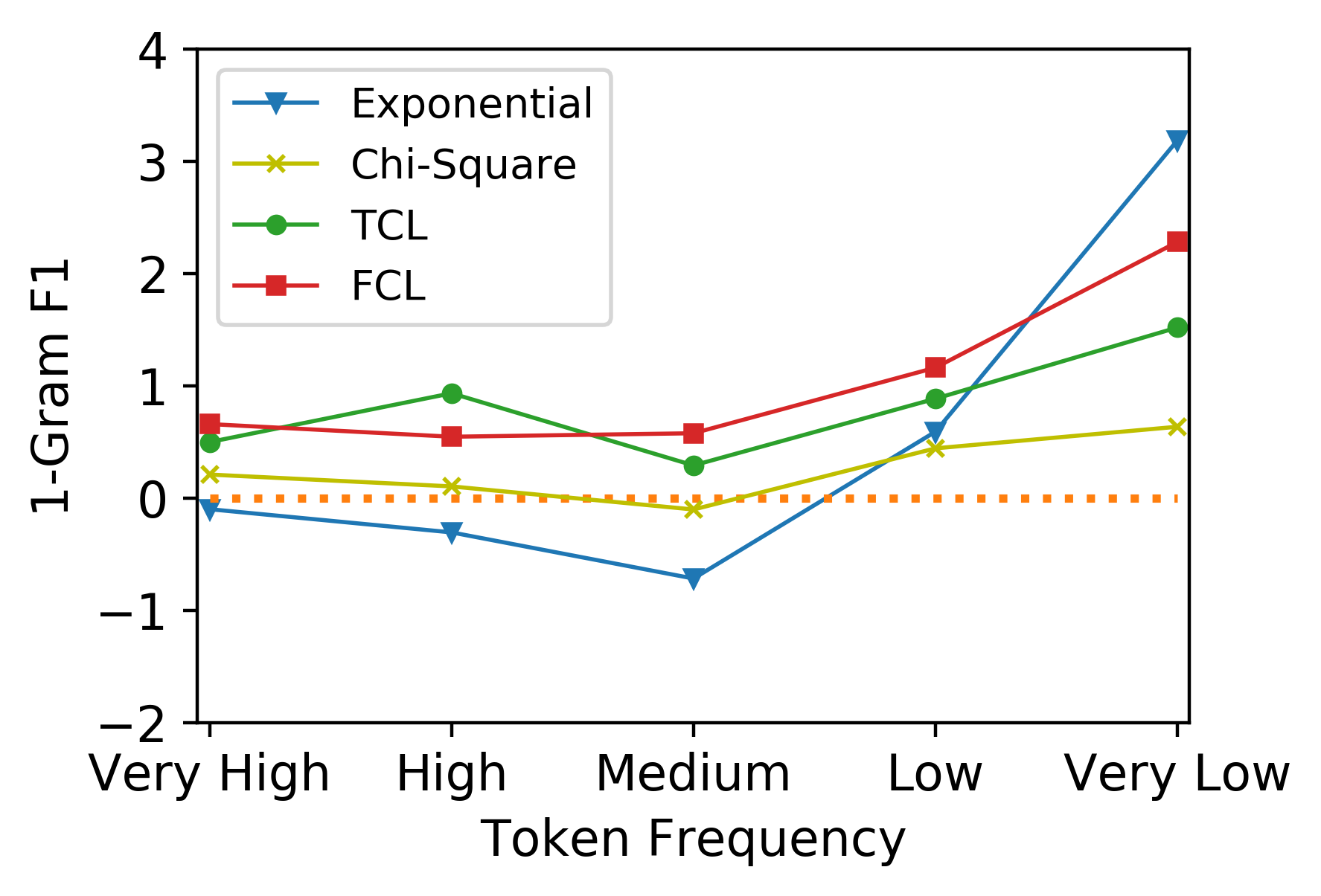
(c) 1-Gram F1 Gap

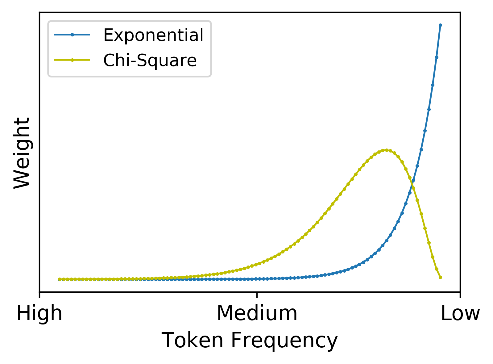
(d) Adaptive Weighting Functions

Figure 3: (a)/(b)/(c) The 1-Gram Recall/Precision/F1 gaps between various models and transformer. The horizontal dashed line means the Transformer baseline. (d) The Exponential and Chi-Square weighting functions in Gu et al. (2020) with descending token frequency. As seen, our methods consistently recall more tokens across different frequencies, in the meanwhile, maintaining the preciseness of prediction.

5.2 Effects on Translation Quality of Low-Frequency Tokens

In this section, we investigate the translation quality of low-frequency tokens. Here we define a target word as a low-frequency word if it appears less than two hundred times in LDC training set. We then rank the target sentences in NIST test sets by the proportion of low-frequency words and divide them into three subsets: “High”, “Middle”, and “Low”.

The BLEU scores on the three subsets are shown in Table 2, from which we can find a similar trend across all methods that the more low-frequency words in a subset, the more notable the performance improvement. Another two more critical observations are that: (1) FCL and TCL demonstrate their superiority over the adaption training methods across all three subsets of different frequencies. (2) The performance improvements on three subsets we achieved (e.g., 0.84, 1.50, and 2.00 by FCL ) consistently keeps remarkable, while the effects of the adaption training methods on subset “High” and “Middle” are modest. Note that the Exponential objective even brings a performance degradation on “High”. These observations verify that our method effectively improves the translation quality of rare tokens, and suggest that improving representation space could be a more robust and systematic way to optimize predictions of diversified-frequency tokens than adaptive training.

Method	MATTR$\uparrow$	HD-D$\uparrow$	MTLD$\uparrow$
Transformer	86.87	86.13	70.96
Exponential	87.52	86.86	75.77
Chi-Square	87.16	86.44	71.97
BMI	87.33	86.64	74.05
TCL	87.00	86.25	71.81
FCL	87.38	86.71	73.86
$Reference$	88.98	88.23	82.47

Table 3: Lexical diversity of translations on NIST test sets.
$\uparrow$ means greater value for greater diversity. Both the proposed models and the related studies raise the lexical richness.

5.3 Effects on Lexical Diversity

As overly ignoring the infrequent tokens will lead to a lower lexical diversity (Vanmassenhove, Shterionov, and Way 2019), we investigate our methods’ effects on lexical diversity following  Gu et al. (2020) and Xu et al. (2021b). We statistic three lexical diversity metrics based on the translation results on NIST test sets, including moving-average type-token ratio (MATTR)  (Covington and McFall 2010), the approximation of hypergeometric distribution (HD-D) and the measure of textual lexical diversity (MTLD) (McCarthy and Jarvis 2010). The results are reported in Table 3, from which we can observe lexical diversity enhancements brought by FCL and TCL over vanilla Transformer, proving the improved tendency of our method to generate low-frequency tokens.

More importantly, we find that Exponential yields the best lexical diversity, though its overall performance improvement in terms of BLEU is far from ours. This observation inspired us to conduct a more thorough investigation of the token-level predictions, which will be described next.

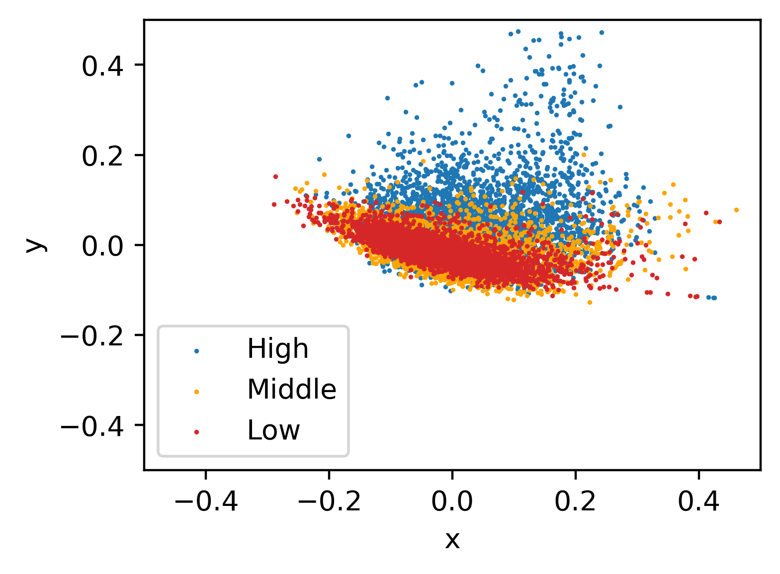
(a) Transformer

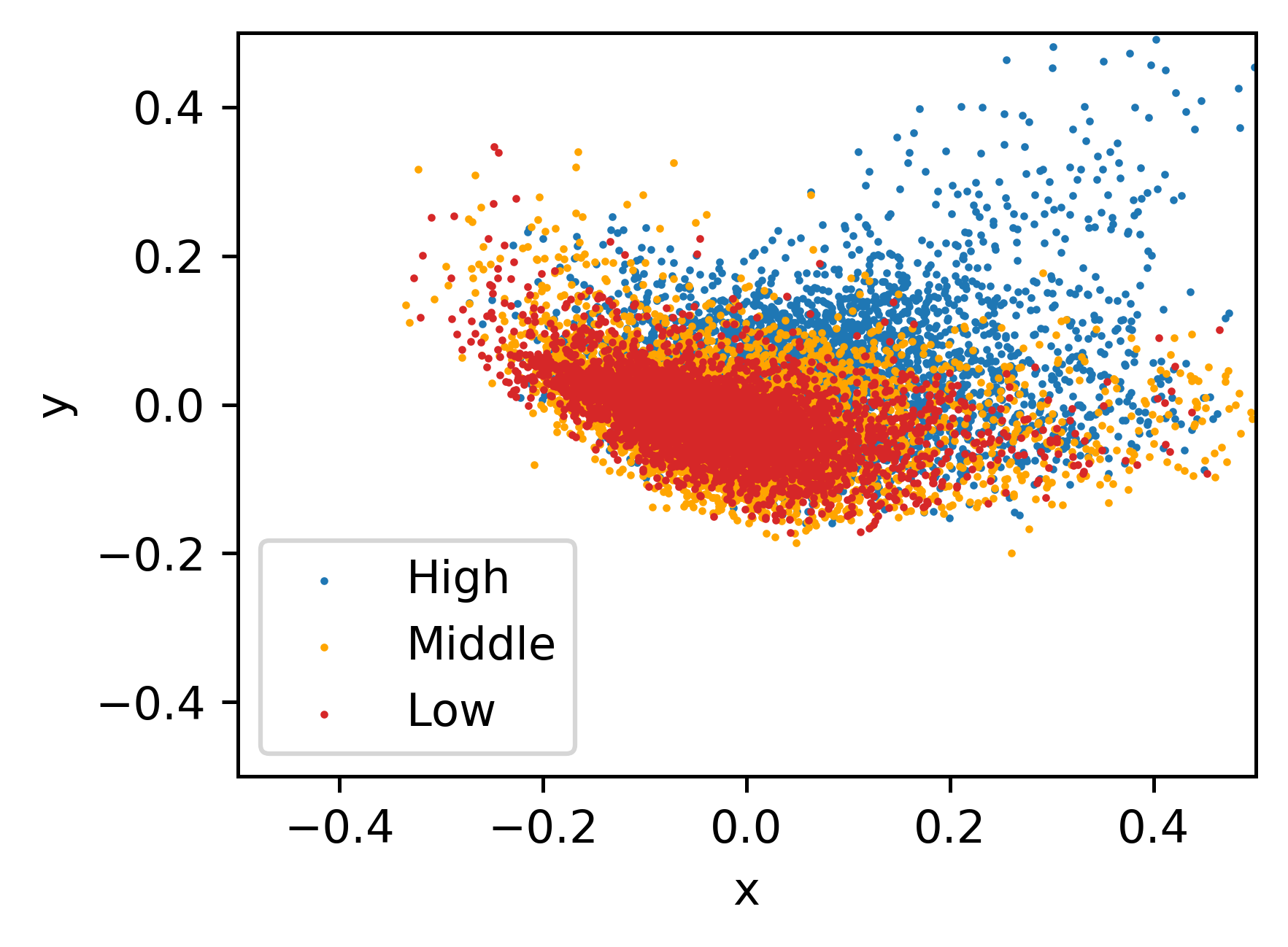
(b) Transformer with TCL

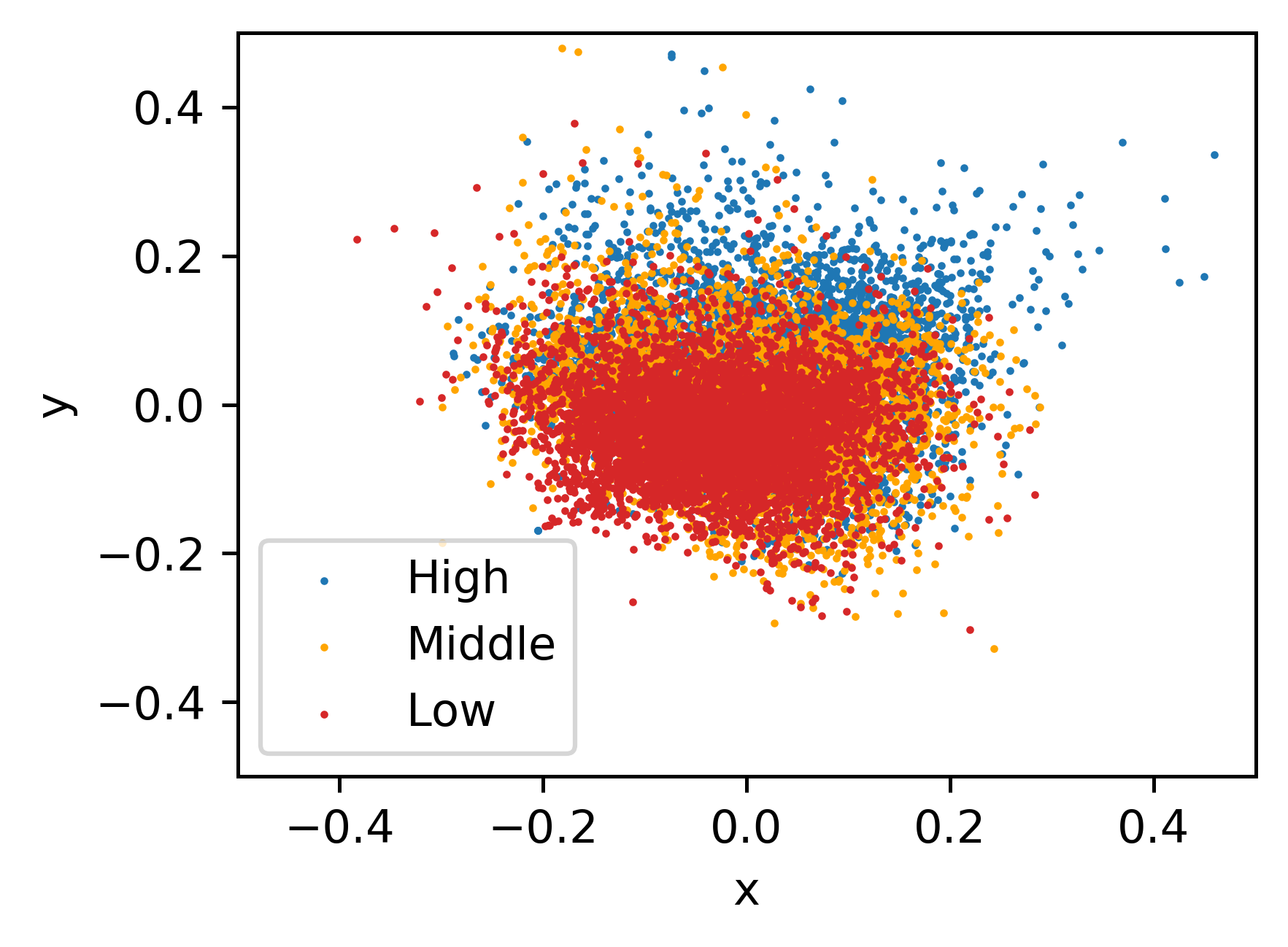
(c) Transformer with FCL

Figure 4: Visualization of word representations (or softmax embeddings) in (a) Transformer, (b) Transformer with TCL, and (c) Transformer with FCL trained on LDC Zh-En dataset. The tokens are evenly divided into three buckets according to the token frequency in the training set. The red dots (“High”) represents the first third of target tokens with high frequency, while the orange and blue ones denote the “Medium” and “Low” buckets, respectively. In baseline system, the rarer the token, the more serious the problem of representation degeneration is. Obviously, the proposed methods progressively alleviate this problem.

5.4 Effects on Token-Level Predictions

Recapping that the three metrics of lexical diversity mainly involve token-level recall, we start by investigating the 1-Gram Recall (or ROUGE-1) of different methods. First, we evenly divide all the target tokens into five groups according to their frequencies, exactly as we did in Figure 1. The 1-Gram Recall results are then calculated for each group, and the gaps between vanilla Transformer and other methods are illustrated in Figure 3 (a) with descending token frequency. Regarding the adaptive training methods, we can more clearly see how different token weights affect the token-level predictions by combing Figure 3 (a) and Figure 3 (d) (plots of the Exponential and Chi-Square weighting functions). Here We mainly discuss based on Exponential for convenience, but note that our main findings also apply to Chi-Square. Generally, we find that 1-Gram Recall enhancement is positively related to the token exposure (or weights), roughly explaining why Exponential achieves the best lexical diversity.

Despite the high 1-Gram Recall of Exponential, its unsatisfied overall performance reminds us that the precision of token-level prediction matters. The 1-Gram Precision results illustrated in Figure 3 (b) verifies our conjecture. Different from the trend in Figure 3 (a), the gaps of Exponential here looks negatively related to the token exposure. This contrast suggests that though the adaptive training methods generate more low-frequency tokens, the generated ones are more likely to be incorrect. Our FCL and TCL, however, maintain the preciseness of token prediction across different frequencies. The 1-Gram Precision improvements of FCL on low-frequency words (Low and Very Low) are even better than high-frequency ones.

Finally, we investigate the 1-Gram F1, a more comprehensive metric to evaluate token-level predictions by considering both 1-Gram Recall and Precision. Based on the polylines shown in Figure 3 (C), we can conclude two distinguished merits of our method compared to the adaptive training methods: (1) enhancing low-frequency word recall without sacrificing the prediction precision and (2) improving token-level predictions across different frequencies consistently, which also confirms the observation in Section  5.2.

5.5 Effects on Representation Learning

Since we approach low-frequency word predictions from a representation learning perspective, we finally conduct two experiments to show how our method impacts word representation, though it is not our primary focus.

Method	-Uni $\uparrow$	Dis $\uparrow$	$I_{1}({\rm\mathbf{W}})\uparrow$	$I_{2}({\rm\mathbf{W}})\downarrow$
Transformer	0.2825	0.3838	0.7446	0.0426
Exponential	0.1148	0.2431	0.7394	0.0432
Chi-Square	0.2276	0.3442	0.7217	0.0425
BMI	0.2118	0.3190	0.7644	0.0430
TCL	0.7024	0.5988	0.7903	0.0399
FCL	0.7490	0.6192	0.7652	0.0394

Table 4: The uniformity and isotropy of softmax embeddings on LDC Zh-En machine translation. $\uparrow$ means a positive correlation with the uniformity of the representation and $\downarrow$ represents a negative correlation to the contrary. Our methods can generate more expressive representations.

Table 4 summarizes the uniformity (Uni) (Wang and Isola 2020), average distance (Dis) as well as the two isotropy criteria $I_{1}({\rm\mathbf{W}})$ and $I_{2}({\rm\mathbf{W}})$ (Wang et al. 2020) of the word embedding matrix in NMT systems. Compared with the Transformer baseline and the adaptive training methods, our TCL and FCL substantially improve the measure of uniformity and isotropy, revealing that the target word representations in our contrastive methods are much more expressive.

To further examine the word representation space, we look at the 2-dimensional visualizations of softmax embeddings by principal component analysis (PCA). One obvious phenomenon in Figure 4 (a) is that the tokens with different frequencies lie in different subregions of the representation space. Meanwhile, the embeddings of low-frequency words are squeezed into a more narrow space, which is consistent with the representation degeneration phenomenon proposed by Gao et al. (2019).

For TCL in Figure 4 (b), this problem is alleviated by the token-level contrast of hidden representations, while the differences in word distribution with different word frequencies still persist. As a comparison shown in Figure 4 (c), our frequency-aware contrastive learning methods that highlight the contrast of infrequent tokens can produce a more uniform and frequency-robust representation space, leading to the inherent superiority in low-frequency word prediction.

6 Conclusion

In this paper, we investigate the problem of low-frequency word prediction in NMT from the representation learning aspect. We propose a novel frequency-aware contrastive learning strategy which can consistently boost translation quality for all words by meliorating word representation space. Via in-depth analyses, our study suggests the following points which may contribute to subsequent researches on this topic: 1) The softmax representations of rarer words are distributed in a more compact latent space, which correlates the difficulty of their prediction; 2) Differentiating token-level hidden representations of different tokens can meliorates the expressiveness of the representation space and benefit the prediction of infrequent words; 3) Emphasizing the contrast for unusual words with frequency-aware information can further optimize the representation distribution and greatly improve low-frequency word prediction; and 4) In rare word prediction, both recall and precision are essential to be assessed, the proposed 1-Gram F1 can simultaneously consider the two aspects.

References

- Arthur, Neubig, and Nakamura (2016) Arthur, P.; Neubig, G.; and Nakamura, S. 2016. Incorporating Discrete Translation Lexicons into Neural Machine Translation. In EMNLP.
- Bahdanau, Cho, and Bengio (2015) Bahdanau, D.; Cho, K.; and Bengio, Y. 2015. Neural Machine Translation by Jointly Learning to Align and Translate. In ICLR.
- Chen et al. (2020) Chen, T.; Kornblith, S.; Norouzi, M.; and Hinton, G. E. 2020. A Simple Framework for Contrastive Learning of Visual Representations. ICML.
- Covington and McFall (2010) Covington, M. A.; and McFall, J. D. 2010. Cutting the Gordian Knot: The Moving-Average Type–Token Ratio (MATTR). Journal of quantitative linguistics, 17(2): 94–100.
- Fang et al. (2020) Fang, H.; Wang, S.; Zhou, M.; Ding, J.; and Xie, P. 2020. CERT: Contrastive Self-Supervised Learning for Language Understanding. arXiv preprint arXiv:2005.12766.
- Feng et al. (2020) Feng, Y.; Xie, W.; Gu, S.; Shao, C.; Zhang, W.; Yang, Z.; and Yu, D. 2020. Modeling Fluency and Faithfulness for Diverse Neural Machine Translation. In AAAI.
- Gao et al. (2019) Gao, J.; He, D.; Tan, X.; Qin, T.; Wang, L.; and Liu, T.-Y. 2019. Representation Degeneration Problem in Training Natural Language Generation Models. In ICLR.
- Gao, Yao, and Chen (2021) Gao, T.; Yao, X.; and Chen, D. 2021. SimCSE: Simple Contrastive Learning of Sentence Embeddings. arXiv preprint arXiv:2104.08821.
- Gowda and May (2020) Gowda, T.; and May, J. 2020. Finding the Optimal Vocabulary Size for Neural Machine Translation. In EMNLP: Findings, 3955–3964.
- Gu et al. (2020) Gu, S.; Zhang, J.; Meng, F.; Feng, Y.; Xie, W.; Zhou, J.; and Yu, D. 2020. Token-Level Adaptive Training for Neural Machine Translation. In EMNLP, 1035–1046.
- Hakan, Khashayar, and Richard (2017) Hakan, I.; Khashayar, K.; and Richard, S. 2017. Tying Word Vectors and Word Classifiers: A Loss Framework for Language Modeling. In ICLR.
- Hjelm et al. (2019) Hjelm, R. D.; Fedorov, A.; Lavoie-Marchildon, S.; Grewal, K.; Trischler, A.; and Bengio, Y. 2019. Learning Deep Representations by Mutual Information Estimation and Maximization. ICLR.
- Jiang et al. (2019) Jiang, S.; Ren, P.; Monz, C.; and de Rijke, M. 2019. Improving Neural Response Diversity with Frequency-Aware Cross-Entropy Loss. In The World Wide Web Conference, 2879–2885.
- Khosla et al. (2020) Khosla, P.; Teterwak, P.; Wang, C.; Sarna, A.; Tian, Y.; Isola, P.; Maschinot, A.; Liu, C.; and Krishnan, D. 2020. Supervised Contrastive Learning. NeurIPS.
- Koehn (2004) Koehn, P. 2004. Statistical Significance Tests for Machine Translation Evaluation. In EMNLP.
- Lee, Cho, and Hofmann (2017) Lee, J.; Cho, K.; and Hofmann, T. 2017. Fully Character-Level Neural Machine Translation without Explicit Segmentation. Transactions of the Association for Computational Linguistics, 5: 365–378.
- Lee, Lee, and Hwang (2021) Lee, S.; Lee, D. B.; and Hwang, S. J. 2021. Contrastive Learning with Adversarial Perturbations for Conditional Text Generation. In ICLR.
- Lin (2004) Lin, C.-Y. 2004. ROUGE: A Package for Automatic Evaluation of Summaries. In ACL.
- Lin et al. (2021) Lin, H.; Yao, L.; Yang, B.; Liu, D.; Zhang, H.; Luo, W.; Huang, D.; and Su, J. 2021. Towards User-Driven Neural Machine Translation. In ACL.
- Lin et al. (2017) Lin, T.-Y.; Goyal, P.; Girshick, R.; He, K.; and Dollár, P. 2017. Focal Loss for Dense Object Detection. In Proceedings of the IEEE international conference on computer vision, 2980–2988.
- Liu et al. (2021) Liu, X.; Yang, B.; Liu, D.; Zhang, H.; Luo, W.; Zhang, M.; Zhang, H.; and Su, J. 2021. Bridging Subword Gaps in Pretrain-Finetune Paradigm for Natural Language Generation. In ACL.
- Logeswaran and Lee (2018) Logeswaran, L.; and Lee, H. 2018. An Efficient Framework for Learning Sentence Representations. ICLR.
- Luong and Manning (2016) Luong, M.-T.; and Manning, C. D. 2016. Achieving Open Vocabulary Neural Machine Translation with Hybrid Word-Character Models. arXiv preprint arXiv:1604.00788.
- Luong et al. (2015) Luong, M.-T.; Sutskever, I.; Le, Q.; Vinyals, O.; and Zaremba, W. 2015. Addressing the Rare Word Problem in Neural Machine Translation. In ACL.
- McCarthy and Jarvis (2010) McCarthy, P. M.; and Jarvis, S. 2010. MTLD, vocd-D, and HD-D: A Validation Study of Sophisticated Approaches to Lexical Diversity Assessment. Behavior research methods, 42(2): 381–392.
- Pan et al. (2021) Pan, X.; Wang, M.; Wu, L.; and Li, L. 2021. Contrastive Learning for Many-to-many Multilingual Neural Machine Translation. In Zong, C.; Xia, F.; Li, W.; and Navigli, R., eds., ACL/IJCNLP.
- Sennrich, Haddow, and Birch (2016) Sennrich, R.; Haddow, B.; and Birch, A. 2016. Neural Machine Translation of Rare Words with Subword Units. In ACL.
- Sutskever, Vinyals, and Le (2014) Sutskever, I.; Vinyals, O.; and Le, Q. V. 2014. Sequence to Sequence Learning with Neural Networks. NeurIPS.
- Vanmassenhove, Shterionov, and Way (2019) Vanmassenhove, E.; Shterionov, D.; and Way, A. 2019. Lost in Translation: Loss and Decay of Linguistic Richness in Machine Translation. In Proceedings of Machine Translation Summit XVII: Research Track, 222–232. Dublin, Ireland: European Association for Machine Translation.
- Vaswani et al. (2017) Vaswani, A.; Shazeer, N.; Parmar, N.; Uszkoreit, J.; Jones, L.; Gomez, A. N.; Kaiser, Ł.; and Polosukhin, I. 2017. Attention is All You Need. In NeurIPS.
- Wan et al. (2020) Wan, Y.; Yang, B.; Wong, D. F.; Zhou, Y.; Chao, L. S.; Zhang, H.; and Chen, B. 2020. Self-Paced Learning for Neural Machine Translation. In EMNLP.
- Wang et al. (2020) Wang, L.; Huang, J.; Huang, K.; Hu, Z.; Wang, G.; and Gu, Q. 2020. Improving Neural Language Generation with Spectrum Control. In ICLR.
- Wang and Isola (2020) Wang, T.; and Isola, P. 2020. Understanding Contrastive Representation Learning through Alignment and Uniformity on the Hypersphere. In ICML.
- Wu et al. (2016) Wu, Y.; Schuster, M.; Chen, Z.; Le, Q. V.; Norouzi, M.; Macherey, W.; Krikun, M.; Cao, Y.; Gao, Q.; Macherey, K.; et al. 2016. Google’s Neural Machine Translation System: Bridging the Gap Between Human and Machine Translation. arXiv preprint arXiv:1609.08144.
- Xu et al. (2021a) Xu, L.; Yang, B.; Lv, X.; Bi, T.; Liu, D.; and Zhang, H. 2021a. Leveraging Advantages of Interactive and Non-Interactive Models for Vector-Based Cross-Lingual Information Retrieval. arXiv preprint arXiv:2111.01992.
- Xu et al. (2021b) Xu, Y.; Liu, Y.; Meng, F.; Zhang, J.; Xu, J.; and Zhou, J. 2021b. Bilingual Mutual Information Based Adaptive Training for Neural Machine Translation. In Zong, C.; Xia, F.; Li, W.; and Navigli, R., eds., ACL/IJCNLP.
- Yang et al. (2019) Yang, Z.; Cheng, Y.; Liu, Y.; and Sun, M. 2019. Reducing Word Omission Errors in Neural Machine Translation: A Contrastive Learning Approach. In ACL.
- Zhang et al. (2017) Zhang, J.; Ding, Y.; Shen, S.; Cheng, Y.; Sun, M.; Luan, H.; and Liu, Y. 2017. Thumt: An open source toolkit for neural machine translation. arXiv preprint arXiv:1706.06415.
- Zhang et al. (2021) Zhang, T.; Zhang, L.; Ye, W.; Li, B.; Sun, J.; Zhu, X.; Zhao, W.; and Zhang, S. 2021. Point, Disambiguate and Copy: Incorporating Bilingual Dictionaries for Neural Machine Translation. In ACL/IJCNLP.
- Zhou et al. (2020) Zhou, Y.; Yang, B.; Wong, D. F.; Wan, Y.; and Chao, L. S. 2020. Uncertainty-aware curriculum learning for neural machine translation. In ACL.
- Zipf (1949) Zipf, G. 1949. Human Behavior and The Principle of Least Effort.