Abstract

We explore supersymmetric SO(10) models predicting observable proton decay and various topological defects which produce different shapes and strengths of gravitational wave backgrounds depending on the scales of intermediate symmetry breaking and inflation as well. We compare these to their non-supersymmetric counterparts. By identifying the scales at which gravitational wave signals appear, we would be able to track down a particular breaking chain and discern if it has a supersymmetric origin or not. It would also be useful to observe gravitational waves from more than one source among all possible topological defects and first order phase transitions for a realistic breaking chain. For these purposes, we work out specific examples in which the grand unification and relevant intermediate scales are calculable explicitly. It turns out that examples with gravitational waves from different sources are quite difficult to obtain, and the predicted gravitational wave profiles from domain walls and first order phase transitions obtained in some examples will require detectors in the kHz to MHz region.

1 Introduction

The first ever direct detection of a gravitational wave (GW) signal in 2015 [1] opened the era of gravitational wave astronomy and revived interests in cosmological GW signals. The study of GW signals from cosmological origin, either topological defects or phase order first transitions (FOPT), is a long standing subject, but only recently the current and future experiments have the potential to detect these kind of signals. During the next years, KAGRA [2] and LIGO-India will be integrated in the LIGO [3, 4, 5, 6] and Virgo [7] interferometer network (LVC). Thanks to the improved sensitivity, a huge number of GW events will be detected. The detection could be so frequent that the associated signals would be too entangled to be identify individually. These events will then appear as a Stochastic Gravitational Wave Background (SGWB), a signal continuous in time, loud in a very broad frequency band, and coming from the whole sky dome. In fact, these are also the characteristics of GW signals created at the earliest moments of the universe. Such signals, called SGWB of Cosmological Origin (SGWBoCO), exist but we do not know their strength and the frequencies at which we could detect them. It is then crucial to design SGWB searches suitable for scenarios where the SGWBoCO and SGWB of astrophysical origin (SGWBoAO) are both present at some level. This kind of searches will need to be implemented by all current and projected experiments, such as LISA TianQin [9], Taiji [10], LISA [11], Einstein Telescope [12, 13], Cosmic Explorer [14], BBO [15] and DECIGO [16], as well as Pulsar Timing Array (PTA) experiments SKA [17], EPTA [18], PPTA [19], IPTA [20]. In fact, in September 2020 the NANOGrav Collaboration announced their PTA analysis [21] showing that we are likely on the verge of a SGWB detection. In particular, it has hinted at the detection of a cosmic string in the range $G\mu\in[2\times 10^{-11},3\times 10^{-10}]$ [22]. A firm SGWB observation may require only some extra years of measurements, and it is encouraging to have the recent positive development of the PPTA analysis [23] and the collaborative effort of IPTA [24]. If confirmed, the NANOGrav SGWB signal in the range $G\mu\in[2\times 10^{-11},3\times 10^{-10}]$ would be compatible with the SGWBoCO produced by (Nambu Goto) cosmic strings coming from a phase transition that occurred between $10^{-22}$ and $10^{-18}$ seconds after the Big Bang.

On the theoretical side, model building within the context of Grand Unified Theories (GUT) needs to provide a compelling science case for scenarios where the cosmological signal can be clearly identified. In this respect, there has been a large number of recent studies reviving the study of GW coming from topological defects . These include non-supersymmetric GUT theories in connection to proton decay and unification [31, 32, 33] and different interconnections to $B-L$ [34], neutrino masses and leptogenesis [35], as well as in connection to addressing the NANOGrav hint for cosmic strings [36, 37] and combined effects with FOPT and GW [38].

In this paper, we address the question if different breaking chains of the supersymmetric SO(10) GUT predicting a certain combination of topological defects and first order phase transition (FOPT) can be identified through the detection of SGWB. This task of course can be done taking into account low energy phenomenological constraints (proton decay, masses, flavor effects, etc.) and assumptions about how inflation should take place.

The classification of breaking routes of SO(10) down to Standard Model (SM), or Minimal Supersymmetric SM (MSSM), producing topological defects, started long time ago [27]. As it is well-known, non-supersymmetric models can yield gauge coupling unification with different intermediate scales [39] and therefore it is appealing to study the GW panorama in this context. Making a catalogue of surviving breaking chains coming from SO(10) models as in [32, 33] is considerably more challenging in supersymmetry due to the fact that not only the number of constraints and parameters is considerably bigger but also to the assumptions for the way supersymmetry is broken and the way it is UV completed. For these reasons we present in this work only a few typical examples, rather than a comprehensive catalogue.

Supersymmetric models can be compared with their non-supersymmetric counterparts because they differ in their breaking scales and proton decay channels and this can be contrasted in the future with both GW and proton decay experiments. We provide a study for this comparison by considering examples based on the SO(10) breaking routes containing the SU(5) and $\text{SU(3)}_{C}\times\text{SU(2)}_{L}\times\text{SU(2)}_{R}\times\text{U(1)}_{B-L}$ sub-groups. These models are representatives of different subgroups and low energy phenomenology and therefore can shed light on discerning routes down to the SM. We envision plots for frequency vs. density showing all possible combination of topological defects and FOPT for a particular breaking chain. Unfortunately, this task is quite model-dependent and will require future developments of simulations, in particular, for hybrid topological defects since the relative tensions of the topological defects is crucial to the evolution of the networks. Nevertheless, it is worth to establish possible breaking routes where hybrid topological defects can leave a distinct GW imprint. Recently, these observations have been also revived in [42] with a similar motivation to ours.

The paper is organized as follows. In section 2 we put into context the appearance of topological defects according to the different breaking routes down to the SM. In section 3 we mention how do we obtain the scale of breaking and how do we compute the proton decay ratios. In section 4 we analyze our model examples and compare to the non-supersymmetric counterparts. In section 5 we conclude. For the sake of completeness, we provide the information that we use to generate the GW signals in the appendices.

2 GUT breaking and topological defects

In this section, we make a brief summary of topological defects appearing in a GUT breaking chain which we use and refer to. Then, we introduce typical SO(10) GUT breaking patterns for which we study various phenomenological features and GW signals from relevant topological defects and possible phase transitions.

2.1 Theory of topological defects in breaking chains

A schematic breaking chain of a GUT model down to the SM can be depicted as

$$G_{\text{GUT}}\ \xrightarrow[]{p_{1},p_{2},\ldots}\ H_{1}\xrightarrow[]{q_{1},q_{2},\ldots}\ H_{2}\ \ldots\ \xrightarrow[]{r_{1},r_{2},\ldots}\ H_{n}\ \xrightarrow[]{s_{1},s_{2},\ldots}\ G_{\rm{SM}},$$ (1)

where the letters $p_{i}$, $q_{i}$ and $r_{i}$ represent topological defects. The conditions for the formation, evolution and stability of topological defects has been thoroughly studied . The $k-$homotopy group, $\pi_{k}(G/H)$, of the vacuum manifold $\mathcal{M}=G/H$ determines the appearance of topological defects since $\pi_{k}(G/H)$ classifies the distinct topological spaces of $G/H$ that appear after the breaking of $G\rightarrow H$. They correspond to $k=3$ for textures, $k=2$ for monopoles, $k=1$ for cosmic strings (CS) and $k=0$ for domain walls (DW), although formally $\pi_{0}$ is not a group: it represents merely the number of connected components of the manifold. If the homotopy groups are trivial, that is, $\pi_{k}(G/H)=I$, then there are no associated defects. The general features of topological defects from the breaking sequence of Eq. (1) can be summarized as follows.

1. The topological defects will be stable up to the $H_{n}$ group if the k-homotopy group of the manifold $G_{\rm{GUT}}/H_{n}$ is not trivial, that is if $\pi_{k}\left(G_{\rm{GUT}}/H_{n}\right)\neq I$; and unstable up to the $H_{n}$ group if the k-homotopy group of the manifold $G_{\rm{GUT}}/H_{n}$ is trivial, that is if $\pi_{k}\left(G_{\rm{GUT}}/H_{n}\right)=I$. The same applies for the manifold $G_{\rm{GUT}}/\left(SU(3)_{C}\times U_{Y}(1)\right)$ which will determine stable or unstable topological defects all the way down to the EW scale.

2. There can appear metastable defects that decay quantum mechanically with a decay rate $\propto e^{-{\mathcal{A}}/\hbar}$, where $\mathcal{A}$ is the “tunneling action” of the particular defect [43]. For the strings decaying via a pair of monopole/anti-monopole the decay rate, which is specifically the tunneling rate per unit string length, $\ell$, is given by

   $$\frac{dP}{d\ell}=\Gamma=\frac{\mu}{2\pi}e^{-\pi\,k},\quad k=\frac{m^{2}}{\mu},\,$$ (2)

   where $\mu$ is the CS tension and $m$ is the scale at which the monopoles are begin created. This means that the creation of strings should not take place much below the formation of monopoles as only decays for values of $k=O(1)$ render a non negligible value of $\Gamma$, since the exponential in Eq. (2) decays rapidly. For values much greater than 1, the decaying cosmic strings become indistinguishable from stable strings. In certain cases, the probability per unit area of a domain wall decaying by the nucleation of strings, goes like [44, 43]

   $$\frac{dP}{dA}\sim\sigma\,e^{-16\pi/3\,\mu^{3}/\sigma^{2}},$$ (3)

   where $P$ is the probability of nucleation and $A$ is the unit area, $\sigma$ and $\mu$ are respectively the tension of the domain wall and the cosmic string. Hence, depending on the tunneling process or the decay time, the metastable defects could appear as (almost) stable or disappear quickly and hence leave different GW background imprints.

3. Hybrid topological defects appear when a defect associated with the homotopy $\pi_{k}(H_{i}/H_{j})$ is produced at a breaking stage and at a subsequent breaking stage a defect with a homotopy $\pi_{k-1}(H_{j}/H_{\ell})$ is generated. Then, the topological defects associated to $\pi_{k}(H_{i}/H_{j})$ interact with those associated with $\pi_{k-1}(H_{j}/H_{\ell})$ [45]. Examples of these phenomena include the well known fact that monopoles could be the seeds of monopole-antimonopole decay of a string via the Schwinger mechanism and also the fact that strings could become the boundaries of the DW produced at a later stage [45, 44, 46]. The interaction and evolution of these defects depend on the tensions and sizes of the interacting defects and on when inflation and reheating take place (see for example [41] for a comprehensive review).

4. If monopoles and cosmic strings are produced at the same breaking step or without any sizable gap, they are unstable [47], but could leave observable GW spectra [48, 40].

5. If domain walls appear together with cosmic stings after inflation, they become unstable due to the attachment of strings and thus leave GW signals without causing a cosmological problem. Furthermore. a discrete symmetry associated with a domain wall could be lifted by Planck mass suppressed terms [49] and thus the domain wall decays to leave an observable GW signature while its cosmological evolution does not conflict with the standard cosmology[50].

Due to the recent development in GW detection, there have been extensive studies of the signatures from the GUT breaking. Distinct GW signals from cosmic strings produced in association with/without monopoles, or around/away from the end of inflation could be detected to provide an important clue of both inflation [51, 52] and GUT theories. A typical U(1) sub-group of SO(10) GUT is $\text{U(1)}_{B-L}$ whose breaking at different scales would be tracked by distinguishing the resulting SGWB [53, 54]. On the other hand, the formation of domain walls and the GW production could be a consequence of the spontaneous breaking of discrete R symmetries [55, 56]. There have been some arguments against the possibility of finding R symmetries [57] in 4D GUT theories. Lastly, the breaking of supersymmetry itself it can lead to FOPT [58] that can generate GW [59].

This makes the study of GW in the context of GUT a fascinating arena that can probe some of the fundamental aspects and predictions of GUTs. As mentioned before, the study of topological defect formation, evolution and production of GW signals has a long history, however more elaborated simulations and treatment of signals are taking place recently given the opportunity for current and future experiments. 

2.2 Typical examples of SO(10) breaking

Here we present possible breaking chains having more than one source of GW signals and that we will analyze in section 4. As it is well-known, uncertainties in determining the parameters involved in the processes of GW production are yet to be greatly reduced. Nevertheless, we can still make qualitative analyses revealing important features. Let us now depict the distinct breaking chains for which we determine the intermediate and unification scales and estimate proton decay ratios:

SO(10) $$\xrightarrow[126~{}(\mbox{\scriptsize{2}})]{\>M_{\text{GUT}}}\text{SU(5)}\times\text{U(1)}_{V}\xrightarrow[45~{}(\mbox{\scriptsize{2}})]{\>M_{R}}\ \text{SU(3)}_{C}\times\text{SU(2)}_{L}\times\text{U(1)}_{V}\times\text{U(1)}_{Z},\xrightarrow[45~{}(\mbox{\scriptsize{1}})]{\>M_{B-L}}G_{\text{SM}}\times\mathbb{Z}_{2}$$ (4)

$$\hskip 227.62204pt\xrightarrow[10]{\>M_{\text{EW}}}\ \text{SU(3)}_{C}\times\text{U(1)}_{Y}\times\mathbb{Z}_{2},$$

SO(10) $$\xrightarrow[45~{}(\mbox{\scriptsize{2}})]{\>M_{\text{GUT}}}\small{\text{SU(3)}_{C}\times\text{SU(2)}_{L}\times\text{SU(2)}_{R}\times\text{U(1)}_{B-L}}\xrightarrow[126~{}(\mbox{\scriptsize{1,pt}})]{\>M_{B-L}}\,G_{\text{SM}}\times\mathbb{Z}_{2}$$ (5)

$$\hskip 227.62204pt\xrightarrow[10]{\>M_{\text{EW}}}\ \text{SU(3)}_{C}\times\text{U(1)}_{Y}\times\mathbb{Z}_{2},$$

SO(10) $$\xrightarrow[210~{}(\mbox{\scriptsize{2,1}})]{\>M_{\text{GUT}}}\small{\text{SU(3)}_{C}\times\text{SU(2)}_{L}\times\text{SU(2)}_{R}\times\text{U(1)}_{B-L}\times D}\xrightarrow[45~{}(\mbox{\scriptsize{0}})]{\>M_{D}}$$ (6)

$$\small{\text{SU(3)}_{C}\times\text{SU(2)}_{L}\times\text{SU(2)}_{R}\times\text{U(1)}_{B-L}}\xrightarrow[126~{}(\mbox{\scriptsize{1}})]{\>M_{B-L}}G_{\text{SM}}\times\mathbb{Z}_{2}$$

$$\hskip 227.62204pt\xrightarrow[10]{\>M_{\text{EW}}}\ \text{SU(3)}_{C}\times\text{U(1)}_{Y}\times\mathbb{Z}_{2}.$$

The numbers (2,1,0) in parentheses denote respectively again topological defects (monopole, string, domain wall), and (pt) means phase transition. The subscripts of the subgroups in Eqs. (4)-(6) are as follows: C for color, L for Left, R for right, $V=4\,I_{R}^{3}-3(B-L)$ and $Z=-I_{R}^{3}+1/2(B-L)$. Where $I_{R}^{3}$ is the third component of the right-handed isospin and $B-L$ the baryon minus the lepton number. The notation $D$ represent the D parity also known as $Z_{2}^{C}$. Note that $\mathbb{Z}_{2}$, which is used in supersymmetry as R-parity, is never broken. Here $\>M_{\text{GUT}}$, $\>M_{R}$ and $\>M_{B-L}$ refer respectively to the GUT scale, the scale where $\text{SU(2)}_{R}$ is broken and the scale where $B-L$ is broken. The forthcoming results of JUNO[61], DUNE [62] and Hyper-Kamiokande [63] experiments will be able to tell us which models are going to be ruled out and therefore this will be able to exclude the models as sources of GW at a particular scale.

One may consider the breaking route of Eq. (5) or Eq. (6) preceded by the Pati-Salam (PS) group $\text{SU(4)}_{C}\times\text{SU(2)}_{L}\times\text{SU(2)}_{R}$, namely adding a PS breaking scale $\>M_{\text{PS}}$ between $\>M_{\text{GUT}}$ and $\>M_{B-L}$ or $\>M_{D}$. However, we find no attainable solutions in the minimal models with $\>M_{\text{GUT}}$ around ($10^{15},10^{16}$) GeV unless $\>M_{\text{GUT}}$ and $\>M_{\text{PS}}$ become the same due to the restricted beta function coefficients of the PS group in the supersymmetric version of the model. More details are provided in Appendix B.

It is indeed interesting to look for breaking chains where combined sources of gravitational waves could appear. It turns out, however, that this does not occur generically. For supersymmetric models with one intermediate step of breaking it is difficult to separate the intermediate scale too much from the unification scale without incurring proton decay problems. With more than one intermediate scale, an intermediate scale could be lowered, e.g., between $10^{10}$ GeV and $10^{13}$ GeV. Then a further splitting of scales can be achieved and combined effects can take place. This is the case for the example in (6). For non-supersymmetric models, the separation of the GUT scale $\>M_{\text{GUT}}$ and any other intermediate scales, $M_{\text{I}}$, $M_{\text{II}}$, is more feasible basically because the number of particles in the theory, which change the coefficients in the beta functions, are much larger than in their supersymmetric counterparts and therefore one can allow more running of the gauge couplings between the intermediate scales. However, it is precisely this hierarchy, i.e. $\>M_{\text{GUT}}\gg M_{\text{I}}$ (or any other intermediate scale $M_{\text{II}}$), that erases potential interactions of combined effects. Specifically, the decay probabilities of Eqs.  (2) and (3) decrease very rapidly because the arguments in the exponential go like $-1\times$ ratios of powers of the masses involved in the breaking chains. For example, for a decaying string at a scale $\sim M_{\text{I}}$, the factor $k$ in Eq. (2) goes like the ratio of $\>M_{\text{GUT}}^{2}/M^{2}_{\text{I}}$, assuming that monopoles are created at $\>M_{\text{GUT}}$. We also note that the example in (eq. 5) allows the signatures both from cosmic strings and from FOPT. However, the signals from domain walls and FOPT turn out to be away from the current sensitivity as it will be shown in section 4.

3 Phenomenological considerations

The minimum set up for studying GUT, and its different breaking chains, calls for computation of unification scales and proton decay depending on the choices of matter content and intermediate scales. Detailed aspects for this are well studied in the context of non-supersymmetric models. When supersymmetry is considered, one needs to make more assumptions about the spectra and boundary conditions. We will take no-scale supergravity boundary conditions following the treatment in [64].

Gauge coupling unification

Except for the cases studied previously in the literature, we compute the beta functions following [65] and express them in the usual form $\mu\,dg_{a}/d\mu=b_{a}^{(1)}/16/\pi^{2}\,g_{a}^{3}$ $+g_{a}^{3}/(16\pi^{2})^{2}$ $\,\left[\sum_{b=1}^{3}\,b_{ab}^{(2)}\,g_{b}^{2}-c_{a}y^{2}_{t}\right]$, where we keep the top Yukawa coupling, $y_{t}$, since due to its relative size in comparison to the gauge couplings it cannot be neglected.

We assume the “survival hypothesis” implying that only the SM particles contribute to the running below the intermediate symmetry breaking scale and all other particles have masses around either $\>M_{\text{GUT}}$ or the intermediate scales.

Proton decay

For non-supersymmetric theories the most sensitive channel is the dimension-6 operator induced decay $p\rightarrow\pi^{0}\,e^{+}$ mediated by gauge fields. We estimate the proton decay for this channel using [66]

$$\Gamma(p\rightarrow\pi^{0}\,e^{+}) = \frac{m_{p}}{32\pi}\left(1-\frac{m^{2}_{\pi^{0}}}{m^{2}_{p}}\right)^{2}\,\left[|\mathcal{A}_{L}(p\rightarrow\,\pi^{0}\,e^{+})|^{2}+|\mathcal{A}_{R}(p\rightarrow\,\pi^{0}\,e^{+})|^{2}\right],$$ (7)

where $m_{p}$ and $m_{\pi^{0}}$ are the proton and the neutron pion, $\pi^{0}$, masses respectively. The amplitude at the weak scale is computed from

$${\mathcal{A}_{L}}(p\rightarrow\pi^{0}\,e^{+}) = C_{RL}((ud)_{R}u_{L})(\mu=2\,\rm GeV)\langle{\it{\pi}}^{0}{\it{|(ud)_{R}u_{R}|p}}\rangle,$$

$${\mathcal{A}_{R}}(p\rightarrow\pi^{0}\,e^{+}) = 2C_{LR}((ud)_{L}u_{R})(\mu=2\,\rm GeV)\langle{\it{\pi}}^{0}{\it{|(ud)_{R}u_{R}|p}}\rangle,$$ (8)

where the Wilson Coefficients $C_{RL}((ud)_{R}u_{L})$ and $C_{LR}((ud)_{L}u_{R})$ corresponds to $C_{1}$ and $C_{2}$ of [66], respectively. For numerical values we use the inputs given in Tab. 1. The most constraining channel for the supersymmetric theories is $p\rightarrow K^{+}\bar{\nu}$, mediated by dimension-5 operators. We use [64]

$$\Gamma(p\rightarrow K^{+}\bar{\nu})=\frac{m_{p}}{32\pi}\left(1-\frac{m^{2}_{K}}{m^{2}_{p}}\right)^{2}|\mathcal{A}(p\rightarrow K^{+}\bar{\nu_{i}})|^{2},$$ (9)

where $m_{K}$ is the mass of the kaon and the decay amplitude is given in terms of the Wilson Coefficients effective at the hadronic scale (2 GeV)

$$\mathcal{A}(p\rightarrow K^{+}\bar{\nu_{i}}) = C_{RL}(usd\nu_{i})\langle K^{+}|(us)_{R}\,d_{L}|p\rangle+C_{RL}(uds\nu_{i})\langle K^{+}|(ud)_{R}\,s_{L}|p\rangle$$ (10)

$$+ C_{LL}(usd\nu_{i})\langle K^{+}|(us)_{L}\,d_{L}|p\rangle+C_{LL}(uds\nu_{i})\langle K^{+}|(ud)_{L}\,s_{L}|p\rangle.$$

It is useful to remember that all of the Wilson Coefficients in Eq. (10) are suppressed by the color-triplet Higgs mass and the supersymmetry breaking scale. The hadronic matrix elements are given in Tab. 1 and the evolution of the Wilson coefficients from $\>M_{\text{GUT}}$ is given in [64].

Experimental/Lattice values used
Parameter	Current Value	Projected Bound	$3\,\sigma$ Discovery
$M_{Z}(M_{Z})$	91.1876 (21) GeV
$\alpha_{S}(M_{Z})$	0.1179(10)
$\alpha_{\rm{e.m.}}(M_{Z})$	1/127.9
$\sin^{2}\theta_{W}(M_{Z})$	0.23121(4)
$m_{t}(m_{t})$	$172.5\pm 0.7$
$\langle\pi^{0}|(ud)_{R}\,u_{L}|p\rangle$	$-0.131(4)(13)$ [67]
$\langle\pi^{0}|(ud)_{L}\,u_{L}|p\rangle$	$0.134(5)(16)$ [67]
$\tau(p\rightarrow\,\pi^{0}\,e^{+})$	$>1.6\times 10^{34}$ yrs [67] [68]	$7.8\times 10^{34}$ yrs $90\%$ C.L [HK[63]]	$6.3\times 10^{34}$ yrs [HK[63]]
	$95\%$ C.L
$\tau(p\rightarrow\,K^{+}\,\bar{\nu})$	$>6.6\times 10^{33}\quad$yrs	$5\times 10^{34}$ yrs [DUNE [62]]
	$95\%$ C.L	$3.2\times 10^{34}$ yrs $90\%$ C.L. [HK[63]]	$2\times 10^{34}$ yrs [HK[63]]

Table 1: Experimental/lattice values used to obtain values of gauge coupling unification and proton decay rates.

The forthcoming experiments DUNE [62], JUNO [61] and Hyper-Kamiokande [63] are expected to improve the current sensitivity by an order of magnitude (see Tab. 1).

4 Results for Different Breaking Chains

4.1 $\mathbf{SU(5)}$ routes

Non-supersymmetric models via SU(5) routes are quite restricted by the proton decay bound in the channel $p\rightarrow\pi^{0}\,e^{+}$ since the Wilson coefficients are suppressed only by the masses of heavy gauge fields: $C_{i}\propto 1/M^{2}_{X}$ (for a review see for example [69].) Thus, the discussion below is specific to supersymmetric SO(10). The following routes are candidates for the appearance of combined effects:

$$\text{SO(10)}\,\rightarrow\,\text{SU(5)}\times\mathbb{Z}_{2}\,\rightarrow\,G_{\text{SM}}\times\mathbb{Z}_{2},$$ (11)

$$\text{SO(10)}\,\rightarrow\,\text{SU(5)}_{F}\times\text{U(1)}_{V}\,\rightarrow\,G_{\text{SM}}\times\mathbb{Z}_{2},$$ (12)

$$\text{SO(10)}\,\rightarrow\,\text{SU(5)}\times\text{U(1)}_{V}\,\rightarrow\,\text{SU(3)}_{C}\times\text{SU(2)}_{L}\times\text{U(1)}_{Z}\times\text{U(1)}_{V}\,\rightarrow\,G_{\text{SM}}\times\mathbb{Z}_{2}.$$ (13)

The first one, Eq. (11), produces cosmic strings at the first step of breaking, and monopoles at the second stage of breaking. As monopoles need to be inflated away, the only GW signal would be due to a possible breaking of R-parity ($\mathbb{Z}_{2}$) or FOPT. The second possibility, Eq. (12), produces monopoles at the first stage of breaking and cosmic strings at the second stage of breaking. However, the proton decay bound requires both breaking scales to be at the same scale close to $10^{16}$ GeV. Thus, inflation needs to take place after that, leaving no imprint from GW, other than the possible $\mathbb{Z}_{2}$ breaking. Note however that the situation can be different in the flipped models. The breaking of $\text{SU(5)}_{F}\times\text{U(1)}_{V}$ (and thus one U(1) factor) can occur at a much lower scale than $10^{16}$ GeV, if we introduce a pair of vector-like particles [70]. For the third route, Eq. (13), monopoles will be produced in the first two breaking steps, while cosmic strings in the last one. Here unification also requires all the three scales to be close to $10^{16}$ GeV. However, just as in the case of of the flipped SU(5) pair of vector-like fields could be introduced to split the scales [70].

In supersymmetric models, the dimension-5 operator in the channel $p\rightarrow K^{+}\bar{\nu}$ is mediated by the exchange of colour-triplet Higgs and suppressed by the scale of supersymmetric particles, $M_{S}$, so effectively the operators mediating proton decay are proportional to $\propto 1/(\>M_{\text{GUT}}\,M_{S})$. This means that we can push up the supersymmetric scale to aid overcoming the present bounds [71, 64]. To have an idea we can write, [69],

$$\tau\sim 4\times 10^{35}\times\sin^{4}(2\beta)\times\left(\frac{0.1}{\overline{A}_{R}}\right)^{2}\,\left(\frac{M_{S}}{100\,\rm{TeV}}\right)^{2}\left(\frac{M_{HC}}{10^{16}\,\rm{GeV}}\right)^{2}\,\rm{yrs.},$$ (14)

where $M_{S}$ is the supersymmetry breaking scale, $M_{HC}$ is the colour-triplet Higgs mass, $\overline{A}_{R}$ is a hadronic parameter and $\beta$ is the usual angle determined by the ratio of the vacuum expectation values of the two Higgs doublets. For $M_{S}=10$ TeV, we get a suppression of $O(10^{-2})$ in Eq. (14) making the proton decay just compatible with the current bound $\tau(p\rightarrow K^{+}\overline{\nu})>6.6\times 10^{33}$ yrs and thus accessible by the upcoming experiments [61, 62, 63]. However, it is nontrivial and it is quite model dependent to achieve the measured Higgs mass $m_{h}=125$ GeV. This puts additional constraints on the model.

When $\text{U(1)}_{V}$ and $\text{U(1)}_{Z}$ are broken, there can appear $B-L$ proton decay modes through, for example, the operator $d^{c}d^{c}u^{c}LH_{u}$ in supersymmetry [72]. However, the resulting proton decay rate depends on the flavour structure of the model and can be suppressed sufficiently. For our analysis, we adopt the results of Fig. 3 of [64] showing the regions where the proton decay rate is compatible with the bound of the channel $p\rightarrow K^{+}\bar{\nu}$. These regions correspond generally to the mass range of $M_{1/2}\geq 5$ TeV and $M_{0}\geq 7$ TeV. Taking $(M_{1/2},M_{0},\tan\beta,\mu)=$ $(5.5\,\rm{TeV},7.0\,\rm{TeV},5,>0)$, we have the GUT scale of

$$\>M_{\text{GUT}} = 8.2\times 10^{15}\,\text{GeV},$$ (15)

and a proton decay rate of

$$\tau(p\rightarrow K^{+}\bar{\nu})=8.6\times 10^{33}\ \rm{yrs}.$$ (16)

This would requires to break all the chains of Eqs. (11-13) directly to $G_{SM}\times\mathbb{Z}_{2}$ at the GUT scale.

The intermediate scales can be separated away from the GUT scale by altering the unification scale and introducing an effective intermediate scale with the addition of multiplets which affect a bit the running but do not have a great impact in the proton decay rate. This would allow detectable hybrid topological defects appearing in the SU(5) route. As an example, we take the chain Eq. (13) and consider the following two cases:

$$\>M_{\text{GUT}} = \>M_{R}\sim 10^{16}\,{\text{GeV}},\ \>M_{B-L}>10^{14}\,{\text{GeV}},$$

$$\>M_{\text{GUT}} = 10^{16}\,{\text{GeV}},\,\>M_{R}>10^{14}\,{\text{GeV}},\quad\>M_{B-L}\sim 10^{14}\,{\text{GeV}}.$$ (17)

Depending on when the inflation takes place, we may observe different gravitational wave signals. If the reheat temperature $T_{RH}$ is higher than $\>M_{B-L}$, there appear the usual signal of undiluted stable comic strings. In the opposite case $T_{RH}<\>M_{B-L}$, all the defects are diluted away, but sizable string regrowth may occur depending on the conditions. They are basically determined by choosing the parameters that satisfy Eq. (7) of [73]. A brief summary about this is provided in the Appendix (D). Basically we assume a number of long strings with the parameter choice of $\tilde{z}=10^{4}$ which is used in the plot Fig. 1. Another interesting phenomenon is the appearance of observable signals of decaying cosmic strings attached with monopole-antimonopole pairs. The second breaking route of Eq. (17) can realize this possibility as $\>M_{R}$ is slightly above than $\>M_{B-L}$ and the inflation can take place in between, $\>M_{R}>T_{RH}>\>M_{B-L}$. We follow [74] in order to get the profile of the decaying cosmic string. All of these features are illustrated in Fig. 1. Our breaking chain also allows the possibility of $T_{RH}>\>M_{R}>\>M_{B-L}$ which has been known to produce undetectable gravitational signals. For this, we refer the readers to the recent study in [42] .

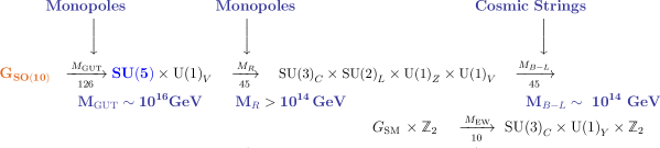
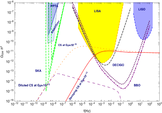
Figure 1: The signals from the breaking of supersymmetric SO(10) via an SU(5) route depending on when the inflation takes place. Taking $\>M_{B-L}=10^{14}$ GeV we show the usual stable CS signal by the dotted orange line, and the diluted CS signal by the dashed purple line. The solid red line shows the decaying CS signal with $\>M_{B-L}=2.5\times 10^{14}$ GeV and $\sqrt{k}=7.5$ (see Eq. (2)). For information about the experimental backgrounds please check Appendix A.

4.2 $\mathbf{SU(3)}_{C}\times\mathbf{SU(2)}_{L}\times\mathbf{SU(2)}_{R}$ $\times\mathbf{U(1)}_{B-L}$

Phenomenological Considerations

Given the breaking chain and the Higgs representations, we use the beta functions given in Appendix B to determine the values of $\>M_{B-L}\!=\!\>M_{R}$ and $\>M_{\text{GUT}}$:

$$\>M_{R}^{2\,\rm{loop}}=(4.2\pm 0.3)\times 10^{13}\,\rm{GeV},$$

$$\>M_{\text{GUT}}^{2\,\rm{loop}}=(1.4\pm 0.26)\times 10^{16}\,\rm{GeV},$$ (18)

where we have computed the uncertainties based only on the parameters of Tab. 1. Adapting the prescription from [75] to our model, we find that the proton decay rate is controlled by the superpotential

$$W_{Y}=\left(Y_{10}^{ij}\mathbf{10}_{\bar{T}}+Y_{126}^{ij}\overline{\mathbf{126}}_{\bar{T}}\right)\,\left(q_{i}l_{j}+u_{i}^{c}\,d^{c}_{j}\right)+\,\left(Y_{10}^{ij}\mathbf{10}_{T}+Y_{126}^{ij}\overline{\mathbf{126}}_{T}\right)\left(\frac{1}{2}q_{i}q_{j}+u^{c}_{i}e^{c}_{j}+d_{i}^{c}\nu^{c}_{j}\right),$$ (19)

where $\mathbf{10}_{\bar{T}}=(\bar{3},1,1,0)+(6,1,1,0)$, $\mathbf{10}_{T}=(3,1,1,0)+(6,1,1,0)$, $\mathbf{126}_{\overline{T}}=(\bar{3},1,1,0)+(6,1,1,0)$, and $\mathbf{126}_{T}=(3,1,1,0)+(6,1,1,0)$, where we have decomposed the SO(10) representations in their $\text{SU(3)}_{C}\times\text{SU(2)}_{L}\times\text{SU(2)}_{R}\times\text{U(1)}_{{B-L}}$ decomposition. All of these representations contain the color triplets and anti-triplets whose masses are denoted by $M_{T}$. To keep supersymmetry unbroken at this stage an additional $\mathbf{126}$ is added. With these modifications we can write the effective dimension-5 operators as in Eq. (6.13) of [75], which is expressed in the following way:

$$C_{L}^{ijkl} = \left(Y_{10}^{ij},Y_{126}^{ij}\right)M_{T}^{-1}\left(\begin{array}[]{c}Y_{10}^{kl},\\ Y_{126}^{kl}\end{array}\right),$$ (22)

$$C_{R}^{ijkl} = \left(Y_{10}^{ij}-f_{1}\,Y_{126}^{ij},f_{2}\,Y_{126}^{ij}\right)M_{T}^{-1}\left(\begin{array}[]{c}Y_{10}^{kl},\\ Y_{126}^{kl}\end{array}\right).$$ (25)

where $f_{1}$ and $f_{2}$ are functions of the vacuum expectation values of $\mathbf{210}$ with $v_{R}=0$ [see Eq. (6.8) of [75]]. The Yukawa couplings $Y_{10}$ and $Y_{126}$ can be written as a linear combination of the up and down quark Yukawa matrices $Y_{u}$ and $Y_{d}$:

$$\left(\begin{array}[]{c}Y_{10}\\ Y_{126}\end{array}\right)=M_{Y}\left(\begin{array}[]{c}Y_{u}\\ Y_{d}\end{array}\right),$$ (30)

where $M_{Y}$ contains the coefficients expressing $Y_{10}$ and $Y_{126}$ as a linear combination of $Y_{u}$ and $Y_{d}$. Once the eigenvalues of the Triplet-Higgs mass $M_{T}$ are found, we use Eq. (30) to rewrite the effective dimension-5 proton decay operators as

$$C_{L}^{ijkl} = \sum_{m=1}^{4}\left(Y_{u}^{ij}A_{m}Y_{u}^{kl}\frac{1}{M_{T_{m}}}+Y_{u}^{ij}B_{m}Y_{d}^{kl}\frac{1}{M_{T_{m}}}\right),$$

$$C_{R}^{ijkl} = \sum_{m=1}^{4}\left(Y_{u}^{ij}C_{m}Y_{u}^{kl}\frac{1}{M_{T_{m}}}+Y_{u}^{ij}D_{m}Y_{d}^{kl}\frac{1}{M_{T_{m}}}\right),$$ (31)

where A, B, C, D are functions of the diagonalization matrices involved in Eq. (22) and Eq. (30). The input values of the quark Yukawa, we use

$$Y_{u}={\text{diag}}(m_{u},m_{c},m_{t})/v/\sin\beta,\quad Y_{d}=V_{CKM}^{*}{\text{diag}}(m_{d},m_{s},m_{b})V^{\dagger}_{CKM}/v/\cos\beta.$$ (32)

We then employ the well known procedure of running and matching the Wilson Coefficients of the relevant Lagrangian at each step. The running of the coefficients $C_{5L,5R}$ from $\>M_{\text{GUT}}$ to $\>M_{B-L}=\>M_{R}$ is governed by

$$\frac{d\,C_{5L,\,CR}^{ijkl}(\mu)}{d\,\ln\mu}=\beta^{Yuk}_{L,R}\,C_{5L,\,5R}^{ijkl}(\mu)\,,$$ (33)

where $\beta^{Yuk}_{L,R}$ are the beta functions of $\text{SU(3)}_{C}\times\text{SU(2)}_{L}\times\text{SU(2)}_{R}\times\text{U(1)}_{{B-L}}$. From $\>M_{B-L}=\>M_{R}$ down to $\>M_{\text{EW}}$, we have the usual running of the Minimal Supersymmetric Standard Model (MSSM) and use the procedure employed in [64]. This means that the coefficients $C_{5R}^{*331i}(\mu)$, $C_{5L}^{jj1k}(\mu)$ are evolved using Eq. (33) from the GUT scale to the supersymmetry breaking scale $M_{S}$. At $M_{S}$, the sfermions are integrated out via the wino- or Higgsino-exchange one-loop diagrams to get the effective Lagrangian $\mathcal{L}^{\rm{eff.}}_{MSSM}=C_{i}^{\tilde{H}}\,O_{1i33}+C_{jk}^{\tilde{W}}\,\widetilde{O}_{1jj3}$ + $C_{jk}^{\tilde{W}}\,\widetilde{O}_{j1jk}+\overline{C}_{jk}^{\tilde{W}}\,\widetilde{O}_{jj1k}$ where the coefficients $C_{i}^{\tilde{H}}$ and $C_{jk}^{\tilde{W}}$ are proportional to $C_{5R}^{*331i}(M_{S})$ and $C_{5L}^{jj1k}(M_{S})$, respectively. Finally, the coefficients of Eq. (10) at the hadronic scale, $C_{RL}(usd\nu_{\tau})$, $C_{RL}(uds\nu_{\tau})$, $C_{LL}(usd\nu_{k})$ and $C_{LL}(uds\nu_{k})$ are proportional to $C_{2}^{\tilde{H}}$, $C_{1}^{\tilde{H}}$, $C_{jk}^{\tilde{W}}$ and $C_{jk}^{\tilde{W}}$, respectively (as given in Eq.  38 of [64]). In order to make a definite evaluation of the proton decay in the $K\,\overline{\nu}$ channel we impose no-scale supergravity conditions at $\>M_{\text{GUT}}$. Then, we look for values of the supersymmetric particles that satisfy the current limits. Taking $M_{0}=1.6\times 10^{4}$ GeV, $M_{1/2}=2\times 10^{4}$ GeV and $\tan\beta=3$, we get

$$\tau(p\rightarrow K\,\overline{\nu})=8.6\,\times 10^{33}\ \rm{yrs},$$ (34)

consistent with the values in Tab. 1.

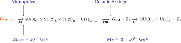
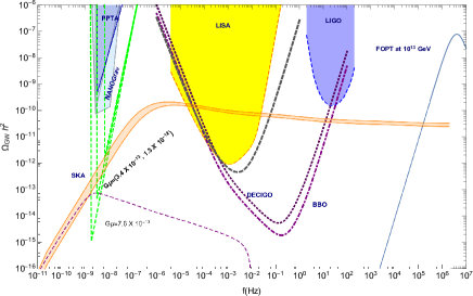
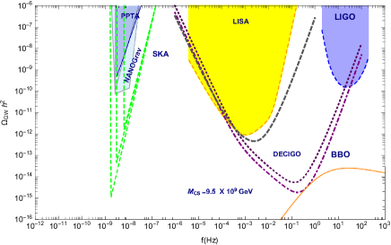
Figure 2: (Left plot: supersymmetric case) The stable CS signal after inflation ($T_{RH}>\>M_{R}$) is shown by the orange band corresponding to $\>M_{R}=(2,4)\times 10^{13}$ GeV. The profile of the diluted CS is shown in the dashed purple line with $\>M_{R}=3\times 10^{13}$ GeV (see the text for the details). The decaying CS signal cannot occur due to the large gap between $\>M_{\text{GUT}}$ and $\>M_{R}$. The blue solid line shows the signal from FOPT at the scale $10^{13}$ GeV which is, unfortunately, out of the future experimental reach. (Right plot: non-supersymmetric case) We show the signals from non-supersymmetric version of the model predicting the intermediate scale at $9.5\times 10^{9}$ GeV corresponding to $G\mu\,=\,7.6\times 10^{-20}$.

First breaking stage

This breaking happens at $\>M_{\text{GUT}}$ given in Eq. (4.2). Monopoles are produced at this scale but no CS.

Second breaking stage

At this scale SU(2) and $\text{U(1)}_{{B-L}}$ are broken and this can happen at the end of inflation. For this case both decaying CS and diluted CS can occur. In the top plot of Fig. 2 we depict the breaking chain which predicts metastable strings after inflation at $10^{13}$ GeV. The scale at which monopoles are produced is $\sim\,10^{16}$ GeV, and thus the string decay rate is exponentially suppressed by the huge number of $k=v^{2}/\mu\sim 10^{6}$ where $v=O(10^{16})$ and $\mu\sim(10^{13}\mbox{GeV})^{2}$ [see Eq. (2)]. Therefore the strings are almost stable and its signature is plotted in the bottom left panel as an orange band corresponding to $(2,4)\times 10^{13}$ GeV. It may happen also that CS are produced during inflation and thus lead to the GW profile of the diluted CS. This is shown in the left bottom panel as a dashed purple line for a redshift of $\tilde{z}=2\times 10^{4}$ that satisfies Eq. (7) of [73].

First Order Phase Transitions

Phase transitions have been analyzed in the context of the present breaking chain and in the context of no-scale supergravity [76], and although they are difficult to realize, there is a possibility and therefore we consider this case. Coleman-Weinberg inflation inflation could also be adopted to achieve FOPT but this has been explicitly carried out only in the context of non-supersymmetric theories [37].

In the bottom-left panel of Fig. 2 we plot a profile of a GW from a FOPT itself at $3\times 10^{13}$ GeV. Note that the predicted GW profile is way out of the present experiment sensitivities. It will require detectors capable to access a frequency band in the kHz to MHz region. In fact, some proposals of exploring up to kHz are starting to take shape, in particular interferometers [77] and optically levitated dielectric sensors spanning a wide frequency band from few kHz to $\sim$ 300 kHz [78, 79]. For the MHz region there are also incipient proposals, [80, 81, 82] for frequencies up to 100 MHz and in the range 1-250 MHZ [83].

The rest of the parameters used to produce the energy density profiles is given in Tab. 2 and the relevant formulas are given in Appendix C.

Parameters used for the FOPT profiles
$\alpha$	$\beta/H$	$g^{*}$	$\epsilon$
$0.9$	1	230	0.1
Parameters used for the DW profile
$\mathcal{A}$	$\tilde{\epsilon}_{GW}$	$g_{*s}(T_{\rm{Ann.}})$	$\sigma$
$0.8$	$0.3$	$230$	$\left((1-3)\times 10^{14}\,\rm{GeV}\right)^{3}$

Table 2: Values of the parameters used to obtain the FOPT profiles of Fig. 2 for $\>M_{R}=4.2\times 10^{13}$ GeV, for which we choose the temperature equal to the corresponding scale. For the supersymmetric DW profile in Fig. 3 we use an annihilation temperature also equal to the a breaking scale of $3\times 10^{14}$ GeV.

Inflation framework

As mentioned before, this breaking pattern has been analyzed in [84, 85], and a Starobinsky-like inflation scenario has been constructed successfully with the inflation energy scale $V_{inf}^{1/4}\approx\,3\times 10^{13}$ GeV which coincides with the scale of the second breaking stage where $B-L$ is broken. Thus, depending on the reheat temperature higher or lower than $\>M_{B-L}$, one can have undiluted or diluted CS signals.

Comparison to Non-Supersymmetric Case

A non-supersymmetric version of this model was considered in [32] taking into account threshold corrections. We have checked the values obtained without threshold corrections to confirm

$$\>M_{R}^{2\,\rm{loop}}=(9.46\pm 1.0)\times 10^{9}\,\rm{GeV},$$

$$\>M_{\text{GUT}}^{2\,\rm{loop}}=(1.60\pm 1.0)\times 10^{16}\,\rm{GeV}.$$ (35)

It is also shown in [32] that the proton decay rate in the channel $p\,\rightarrow\,\pi^{0}\,e^{+}$ is above the current bound, $1.6\times 10^{34}$ yr even without threshold corrections. Future experiments, JUNO[61], DUNE [62] and Hyper-Kamiokande [63], have the potential to exclude it. Note however that threshold corrections or additional singlets added to the theory can push-up the limits [32].

In the right plot of Fig. 2 we show the GW signal from a CS (orange curve in the lower right-corner) that would occur at $9.5\times 10^{9}$ GeV corresponding to the tension of $G\mu\,=\,7.6\times 10^{-20}$). In this non-supersymmetric scenario inflation can take place before that and so the CS will behave like stable string, which is in the reach of BBO.

4.3 $\mathbf{SU(3)}_{C}\times\mathbf{SU(2)}_{L}\times\mathbf{SU(2)}_{R}$ $\times\mathbf{U(1)}_{B-L}\times\mathbf{D}$

Phenomenological Considerations

Now we consider the breaking chain depicted in Fig. 3. This allows three scales of breaking before the breaking to the SM. The first breaking at $\>M_{\text{GUT}}$ is achieved with a $\mathbf{210}$ representation, and the second at $M_{D}$, where D parity is broken, is achieved with a $\mathbf{45}$ representation. At the last scale, $\>M_{R}$, both $SU(2)_{R}$ and $U(1)_{B-L}$ are broken. Thus, depending on $T_{RH}$ higher or lower than $M_{B-L}$, one can have undiluted or diluted CS signals.

We recall the reader that there is no unique solution to $\>M_{\text{GUT}},\>M_{D}$ and $\>M_{R}$. Given one scale, however, the other two are determined. We find specific solutions following the two criteria: (a) $\>M_{D}$ is below $10^{14}$ GeV so that the D parity is broken at a scale compatible with inflation and (b) maximize the GUT scale in order to avoid fast proton decay. The overall ranges of the supersymmetric solutions are

$$\>M_{R}^{2\,\rm{loop}} = (1\times 10^{12},3\times 10^{15})\,\rm{GeV},$$

$$M_{D}^{2\,\rm{loop}} = (1\times 10^{13},1\times 10^{16})\,\rm{GeV},$$

$$\>M_{\text{GUT}}^{2\,\rm{loop}} = (1\times 10^{14},2\times 10^{16})\,\rm{GeV}.$$ (36)

Here, the lowest value of $\>M_{R}$ produces the value of $\>M_{\text{GUT}}=10^{14}$ GeV leading to too fast proton decay. We note also that the split between $\>M_{R}$ and $M_{D}$ is always $O(10)$, and that once $M_{D}$ is close to $10^{16}$ GeV it is indistinguishable from $\>M_{\text{GUT}}$. Out of the possible range of solutions of Eq. (4.3), we look for a solution where $\>M_{\text{GUT}}$ is not smaller than $10^{15}$ GeV to avoid fast proton decay, and $M_{R}$ is not above $10^{14}$ GeV such that the appearance of DW takes place after inflation. For these reasons, we focus on the following solution

$$\>M_{R}^{2\,\rm{loop}} = (3.7\pm 0.2)\times 10^{13}\,\rm{GeV},$$

$$M_{D}^{2\,\rm{loop}} = (3.8\pm 0.2)\times 10^{14}\,\rm{GeV},$$

$$\>M_{\text{GUT}}^{2\,\rm{loop}} = (1.0\pm 0.1)\times 10^{15}\,\rm{GeV},$$ (37)

where we have included uncertainties from the electroweak parameters, $M_{Z}$, $\alpha_{S}$ and $m_{t}$, quoted in Tab. 1. We remark that $M_{D}$ and $\>M_{\text{GUT}}$ tend to be closer to each other, than $M_{R}$ and $M_{D}$ , mainly because of the value of the coefficient $(b^{(1)}_{2L})_{G_{1}}$ with respect to $(b^{(1)}_{2L})_{G_{2}}$, where here $G_{2}=\text{SU(3)}_{C}\times\text{SU(2)}_{L}\times\text{SU(2)}_{R}\times\text{U(1)}_{{B-L}}$ and $G_{1}=\text{SU(3)}_{C}\times\text{SU(2)}_{L}\times\text{SU(2)}_{R}\times\text{U(1)}_{{B-L}}\times D$. These coefficients are such that $(b^{(1)}_{2L})_{G_{1}}>(b^{(1)}_{2L})_{G_{2}}$, both for the symmetric and non-supersymmetric cases. The value of $\>M_{\text{GUT}}$ for this case, Eq. (4.3), drives a fast proton decay unless we set the sparticle masses in the 100 TeV range (see Eq. (14)). At this scale, however the dimension-six operators leading to $p\rightarrow\pi^{0}e^{+}$ become relevant. To calculate proton decay we proceed as in the previous section section 4.2 with two matching scales, $\>M_{D}$ and $\>M_{R}$. For the dimension-six operator, we use the procedure of [64] to obtain the proton lifetime $2\times 10^{34}$ yrs which is just above the current bound (Tab. 1). For the dimension-five operator leading to $p\rightarrow K^{+}\bar{\nu}$, we obtain the proton lifetime $9\times 10^{33}$ yrs with the sparticle masses at 100 TeV, which falls in the reach of the next generation proton decay experiments.

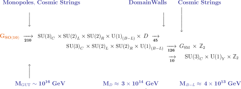
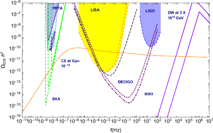
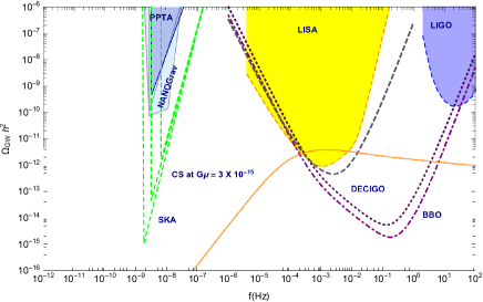
Figure 3: (Left plot: supersymmetric case) The solid purple line represents the profile of a GW generated by a DW after inflation at a scale about $10^{14}$ GeV. We have used the parametric formula of Eq. (98) with the values of Tab. 2. The tension has been taken between $(3\times 10^{14}\,\rm{GeV})^{3}$ (top line) and $(1\times 10^{14}\,\rm{GeV})^{3}$ (bottom line). The solid orange line is the signal from CS produced at about $3.7\times 10^{13}\,\rm{GeV}$, corresponding to $G\mu\,=\,10^{-12}$. (Right plot: non-supersymmetric case) DW are formed above $10^{15}$ GeV and hence are not observable. CS (solid orange line) for this case are produced at $2\times 10^{12}$ GeV, corresponding to a tension $G\mu$ approximately equal to $3\times 10^{-15}$.

GW from Domain Walls

The BICEP2-Kek Array/Planck constraint [86] on inflation sets an upper bound on the Hubble parameter during single-field inflation at $H_{*}<2.5\times 10^{-5}\,\>M_{\text{P}}$ $=3.0\times 10^{14}$ GeV.

This, in turns, sets an upper bound for the scale of this kind of inflation and hence serves as a guide to look for the scales for which topological defects are not completely erased by inflation and reheating.

It is known that the domain wall network can overclose the universe if it is generated after inflation. This can be overcome in various ways (see Appendix E). One possibility is that the formation of cosmic strings takes place just before inflation and the domain wall formation takes place after inflation. Then the strings can nucleate on the wall, which make domain walls to decay through a quantum tunneling process [44, 43]. This process is controlled by the ratio $\mu/\sigma$ between the string tension $\mu$ and the wall tension $\sigma$. If the radius $R$ of a circular string satisfies $R>\mu/\sigma$, the (nucleating a loop of string) rate per unit area is given by Eq. (3).

In the present case where the D parity breaking produces $\mathbb{Z}_{2}$ walls, we can use the results of the existing simulations. These simulations assume that all damping forces that could be present in the cosmological evolution of the string-wall network are negligible and hence the wall tension goes like $\sigma\sim\>M_{D}^{3}$ [41].

We can then use the formula of Eq. (98) to describe the GW signal left by the domain wall. Note that in this case an order of magnitude for the hierarchy between $M_{D}$ and $\>M_{\text{GUT}}$ is enough to produce a large value of $\mu^{3}/\sigma^{2}$ which will make the DW evolution indistinguishable from the evolution of DW without the presence of CS.

In this model, the scale $\>M_{D}=3.8\times 10^{14}$ GeV is of the order of the bound for the Hubble parameter of single-field inflation, as mentioned at the beginning of this section. So in this case the domain walls could have been produced at the end of the inflation leaving their GW as given in Eq. (98). In the left plot of Fig. 3 we plot the DW corresponding to this scale with the rest of the parameters as in Tab. 2.

We recall that our motivation is to look for signals of multiple GW sources coming from topological defects or from FOPT from GUTs. So we ask the following question: suppose that a signal corresponding to the shape and frequency of a DW is reconstructed and has a peak frequency of about $10^{5}$, would this be then indicative of a DW produced by the breaking of a subgroup of a GUT preceded by a breaking producing CS? To put it in other words, we are asking if such a reconstructed signal would be a clear signal of a DW in the presence of CS. To answer the question we recall the following. It is known that DW could be also produced when a symmetry is lifted in the vacuum after the breaking of a discrete parity, such that the effective bias term drives the annihilation of the DW [87, 88, 89]. An specific way to do this is to consider a potential of the form $V=1/4\lambda\,\phi^{4}+\phi^{6}/\Lambda^{2}$ , where $\Lambda$ is a cutoff scale for the dimension 6 operator and $\phi$ represents the Higgs breaking of the $D$ symmetry. In this case, even in the absence of CS, such a term could originate from the $\mathbf{16}$ of SO(10), which under the group $\text{SU(3)}_{C}\times\text{SU(2)}_{L}\times\text{SU(2)}_{R}$ $\times\text{U(1)}_{{B-L}}\times\mathbf{D}$ contains a singlet and hence both of the terms $\phi^{4}$ and $\phi^{6}$ would be allowed. Then, the tension of the string can be estimated from

$$\sigma\sim V^{1/2}_{\rm{max}}\phi_{f},$$ (38)

where $\phi_{f}$ represents the value of the Higgs field where the two minima are quasi-degenerated. At the scale $10^{13}$ GeV the typical values of $V$ and $\phi$ will be respectively $\left(10^{13}\right)^{4}$ and $10^{13}$, giving then as a result a tension $\sigma$ of the order $\left(10^{13}\,\rm{GeV}\right)^{3}$. In this way, DW can collapse and part of their energy will be converted to GW. We can take the annihilation temperature to coincide with the scale of the breaking $10^{13}$ GeV, assuming of course that inflation takes place above that scale. The signal will be indistinguishable from the DW signal that we illustrate in Fig. 3 we present a DW profile, using the parametric formula of Eq. (98) with the parameters appearing in Tab. 2.

Comparison to Non-Supersymmetric Case

Considering the non-supersymmetric model, we find the following ranges for the intermediate scales $\>M_{R}$, $\>M_{D}$, and $\>M_{\text{GUT}}$

$$\>M_{R}^{2\,\rm{loop}}=(1\times 10^{10},5\times 10^{13})\,\rm{GeV},$$

$$\>M_{D}^{2\,\rm{loop}}=(1\times 10^{15},1\times 10^{16})\,\rm{GeV},$$

$$\>M_{\text{GUT}}^{2\,\rm{loop}}=(1\times 10^{15},5\times 10^{16})\,\rm{GeV}.$$ (39)

These values were obtained following the same procedure as in the supersymmetric case. Notice that we do not find any solution with $\>M_{D}$ below $10^{15}$ GeV, and thus $\>M_{D}$ is always above the inflation scale.

The non-supersymmetric counterpart of the model gives the following scales

$$\>M_{R}^{2\,\rm{loop}} = (2.0\pm 0.1)\times 10^{12}\,\rm{GeV},$$

$$\>M_{D}^{2\,\rm{loop}} = (4.0\pm 0.1)\times 10^{15}\,\rm{GeV},$$

$$\>M_{\text{GUT}}^{2\,\rm{loop}} = (7.3\pm 0.1)\times 10^{15}\,\rm{GeV}.$$ (40)

which are to be compared with the supersymmetric case Eq. (15). The big differences in the predicted breaking scales will are maintained even after including the full uncertainties. In this nonsupersymmetric case, domain walls would be formed above $10^{15}$ GeV and hence will not be observable. Cosmic strings can be produced after inflation at a scale $2\times 10^{12}$ GeV, corresponding to approximately to a tension $G\mu=3\times 10^{-15}$. This is plotted in Fig. 3 with a solid orange line. We also checked that the proton lifetime in the $p\rightarrow\pi^{0}e^{+}$ channel is $1.0\times 10^{35}$ yrs which is above the reach of the next generation of experiments (Tab. 1).

5 Conclusions

We studied the possibility of tracking down a route from SO(10) down to the SM in supersymmetric SO(10) models using GW signatures from the topological defects involved in the various stages of breaking, which may differ from the non-supersymmetric counterparts. Non-supersymmetric models have been studied widely as they require various intermediate steps of breaking to achieve gauge unification. Although limited, supersymmetric models may also allow some intermediate breaking scales which could improve gauge coupling unification.

The shapes and strengths of gravitational wave signals depend on the scales of intermediate breaking, the scale of inflation, as well as whether or not hybrid topological defects appear. We explored such features considering the breaking routes of SU(5), $\text{SU(3)}_{C}\times\text{SU(2)}_{R}\times\text{SU(2)}_{L}\times\text{U(1)}_{{B-L}}$ and $\text{SU(3)}_{C}\times\text{SU(2)}_{R}\times\text{SU(2)}_{L}\times\text{U(1)}_{{B-L}}\times D$ with appropriate Higgs representations, and made a comparison between supersymmetric and non-supersymmetric versions. For each case, we determined the values of the GUT and intermediate scales by 2-loop RGE, and computed the rate of proton decay in the most constraining channel $p\rightarrow K^{+}\bar{\nu}$ assuming no-scale supergravity conditions. The resulting GW signals depending on the inflation scale are depicted in Figs. 1, 2 and 3.

In the supersymmetric SU(5) example, the only GW signatures that we could identify are from cosmic strings appearing at the intermediate scale around $10^{14}$ GeV. These could decay due to monopoles predicted in a previous breaking step, or become diluted depending on the scale of inflation. Therefore, variant GW signals are predicted. The breaking routes of SO(10) via $\text{SU(3)}_{C}\times\text{SU(2)}_{R}\times\text{SU(2)}_{L}\times\text{U(1)}_{{B-L}}$ and $\text{SU(3)}_{C}\times\text{SU(2)}_{R}\times\text{SU(2)}_{L}\times\text{U(1)}_{{B-L}}\times D$ offer a broader spectrum of GW signatures.

In the case of $\text{SU(3)}_{C}\times\text{SU(2)}_{R}\times\text{SU(2)}_{L}\times\text{U(1)}_{{B-L}}$ we chose only one intermediate scale, which turns out to be ${\cal O}(10^{13})$ GeV for the supersymmetric case and ${\cal O}(10^{10})$ GeV for the non-supersymmetric case. As these are much lower than the previous breaking scale at which monopoles appear, the monopoles cannot mediate the decay of cosmic strings. However, diluted cosmic strings could appear depending on the inflation scale. For the $\text{SU(3)}_{C}\times\text{SU(2)}_{R}\times\text{SU(2)}_{L}\times\text{U(1)}_{{B-L}}\times D$ example we chose two intermediate scales: $\>M_{D}$ at which D is broken, and $\>M_{R}=\>M_{B-L}$ below which the SM gauge group is obtained. Unlike in the cases with one intermediate scale, a wide range for the first breaking scale is obtained. We focused on the solution where domain walls appear from the $D$ breaking after inflation, which can occur favorably for the supersymmetric case allowing $\>M_{D}={\cal O}(10^{14})$ GeV, and $\>M_{R}={\cal O}(10^{13})$ GeV. On the other hand, the non-supersymmetric model predicts $\>M_{D}\gtrsim 10^{15}$ GeV and $\>M_{R}\lesssim 10^{13}$ GeV. In both cases stable cosmic strings appear below the scale $\>M_{R}$. In the third case, we focused on studying cases where GW from different sources could appear. However, from the range of solutions of Eq. (4.3) it would be possible to choose a value of $\>M_{R}=O(10^{14})$ GeV that could correspond to the range at which the IPTA signal has been observed, $G\mu\in$[$2\times 10^{-11},3\times 10^{-10}$], but inflation and reheating in this case would need to have finished by then.

We conclude by commenting on the reasons why it is difficult to find examples where GW signatures from different sources can appear. Considering only topological defects, we mainly need the breaking of the GUT group down to the SM in at least three steps. The separation of these steps needs to be controlled to assure that the topological defects producing observable GW signals occur after inflation and reheating. These features are illustrated in our breaking chain 4.3. In this case, the appearance of cosmic strings and DW is separated by roughly an order of magnitude, and hence DW decay via nucleation of strings on the wall while avoiding the overclosure of the universe and producing GW at the same time. Thus, two separate GW signals arise: one from DW at a higher scale and the other from CS at a lower scale.

On the other hand, FOPT could occur at any scale and thus two GW signals can arise at a scale below inflation as shown in §4.2. Since monopoles are typically produced at the GUT scale, the scale where GW from FOPT and another source could appear has to be different from the GUT scale and so effectively at least two scales are needed.

Appendix A Confrontation with GW experiments

The GW signals from stochastic backgrounds are by convention expressed in terms of a GW energy density spectrum $\Omega_{\rm{signal}}(f)\,h^{2}$ as a function of the GW frequency $f$, while the instantaneous sensitivity of a GW experiment is expressed as a noise spectrum $\Omega_{\rm{noise}}(f)\,h^{2}$. Then to evaluate if a predicted signal would be able to be detected one can use one of the following procedures. I. Compute the associated signal-to-noise ratio (SNR) by integrating over the experiments’ total observation time accessible to a given frequency [91, 92, 93]: $\text{SNR}^{2}=\,n_{\rm{det}}\,t_{\rm{obs}}\,\int^{f_{\rm max}}_{f_{\rm min}}\,df\,\left[\frac{\Omega_{\rm{signal}}(f)}{\Omega_{\rm{noise}}(f)}\right]^{2}$, where $n_{\rm{det}}$, can be 1 or 2 respectively for a cross-correlation or measurement. Then if SNR is bigger than a threshold value, it is assumed that the associated GW experiment will be able to detect the predicted GW signal. II. Construct the power-law-integrated sensitivity curve (PLISC), $\Omega_{\rm{PLISC}}$, [5] based on $\Omega_{\rm{signal}}(f)$. If the signal and the PLISC intersect in such a way that $\Omega_{\rm{signal}}(f)>$ $\Omega_{\rm{PLISC}}$ for a given frequency, then is assumed that the experiment will be able to detect the signal. However, since the PLISCs are constructed on spectra based on pure power laws, in realistic situations where the signal is expected to have a structure different to a pure power law, PLISCs it can be used only as a qualitative visual aid. In cases where the shape of the predicted GW signal is fairly model independent the computation of SNR can be computed only once. This fact was exploited in [94], where new sensitivity curves for SGWB predicted by FOPT were proposed. The shape of these curves is fairly model independent (the computation depends on the contributions from sound wave and turbulence and their associated parameters). The idea is that using a fit function for a peak-integrated sensitivity curves (PISC) for a particular experiment it is not necessary to perform a frequency integration on a parameter-point-by point basis, but simply plot a numerical fit for the PISC against the predicted SWGB. Updating only when the spectral shape functions, the noise spectrum and the functional forms of the peak amplitude change. Unfortunately PISC have been obtained only for few experiments in particular LISA, DECIGO and BBO and for SGWB FOPT. We compare our examples in section 4 to the profiles of these last experiments based on the information of [94] and for NANOGrav, PPTA and SKA we use smoothed profiles for the sensitivity curves based respectively on [22, 21], [17] and [19], while for LIGO whe use the (PLISCs) [5] approach. As a comparison in our plots we plot the LISA PLISCs and PISC approaches. In all of our plots for LISA, BBO and DECIGO we use $t_{\rm{obs}}=1$ year. For SKA, we present observation times corresponding to one, two and five years, these are shown in the plots appearing in Fig. 1-Fig. 3 respectively as the small, medium and big triangular regions delimited by green dashed lines.

Appendix B Beta Functions

$\mathbf{SU(3)_{C}}\times\mathbf{SU(2)_{L}}\times\mathbf{SU(2)_{R}}\times\mathbf{U(1)_{B-L}}$

For this model the $\mathbf{45}$ breaks the SO(10) group, breaking D parity as well. The $\overline{\mathbf{126}}$ break subsequently to $G_{SM}\times\mathbb{Z}_{2}$ and then the $\mathbf{10}$ makes the breaking at the EW scale. Following the order of the indices as $a=2L,2R,BL,SU(3)_{C}$, for this model the component acquiring vev in the $\mathbf{126}$ is $(1,3,2,1)$ and that of $\mathbf{10}$ is $(2,2,0,1)$ $\supset(2,1,\pm 1/2)$, this last decomposition being the decomposition under the SM group, $SU(2)_{L}\times SU(3)_{C}\times U(1)_{Y}$. For the matter, all fermions and their corresponding sparticles in the $\mathbf{16}$ are taken into account: $(2,1,-1/3,3)$, $(2,1,1,1)$, $(1,2,1/3,\overline{3})$ and $(1,2,-1,1)$. Then the beta functions coefficients at one and two loops are respectively

$$b_{a}^{(1)}=\left(\begin{array}[]{c}1\\ 3\\ 21/2\\ -3\\ \end{array}\right),\quad b_{ab}^{(2)}=\left(\begin{array}[]{cccc}34&8&45&9\\ 1&14&9&9\\ 15&24&49&3\\ 3&24&3&25\end{array}\right),$$ (49)

while for non-supersymmetric, we have

$$b_{a}^{(1)}=\left(\begin{array}[]{c}-3\\ -7/2\\ 11/2\\ -7\\ \end{array}\right),\quad b_{ab}^{(2)}=\left(\begin{array}[]{cccc}8&3&3/2&12\\ 3&80/3&27/2&12\\ 9/2&81/2&61/2&4\\ 9/2&9/2&1/2&-20\end{array}\right).$$ (58)

For the non-supersymmetric case our results agree with those of [66, 32]. The matching conditions at the scale $\>M_{R}$ are as those in Eq. (B).

$\mathbf{SU(3)_{C}}\times\mathbf{SU(2)_{L}}\times\mathbf{SU(2)_{R}}\times\mathbf{U(1)_{B-L}}\times\mathbf{D}$

For this case, the breaking from SO(10) is achieved through a $\mathbf{210}$ representation, which preserves the D symmetry. Then, the $\mathbf{45}$ representation is used to break down to the group $\text{SU(3)}_{C}\times\text{SU(2)}_{R}\times\text{SU(2)}_{L}\times\text{U(1)}_{{B-L}}$. The $\mathbf{126}$ is used to break to the MSSM or the SM group. Finally the $\mathbf{10}$ representation is used for the final breaking at the EW scale. Specifically, the ${\mathbf{126}}\,\supset\,(1,3,2,1)$ makes the subsequent breaking to the MSSM and the $\mathbf{10}\,\supset\,(2,2,0,1)$ to the SM. The order of the indices is also $a=2L,2R,BL,\text{SU(3)}_{C}$. The fermions are in the $\mathbf{16}$ representation $\supset\,(2,1,-1/3,3)$, $(2,1,1,1)$, $(1,2,1/3,\bar{3})$, $(1,2,-1,1)$. The coefficients of the beta functions are as follows:

$$b_{a}^{(1)}=\left(\begin{array}[]{c}3\\ 3\\ 15\\ -3\\ \end{array}\right),\quad b_{ab}^{(2)}=\left(\begin{array}[]{cccc}45&45&61&8\\ 3&3&15&24\\ 49&49&15&24\\ 9&9&1&14\end{array}\right).$$ (67)

The non-supersymmetric beta function coefficients of this example are

$$b_{a}^{(1)}=\left(\begin{array}[]{c}-7/3\\ -7/3\\ 7\\ -7\\ \end{array}\right),\quad b_{ab}^{(2)}=\left(\begin{array}[]{cccc}80/3&3&27/2&12\\ 3&80/3&27/2&12\\ 81/2&81/2&115/2&4\\ 9/2&9/2&1/2&-26\end{array}\right).$$ (76)

Again for these cases, for the non-supersymmetric case, we reproduce the results of [66, 32]. At the scale $\>M_{D}$ then the 45 is used to break D parity and from this scale to the scale $\>M_{R}=\>M_{B-L}$ the beta functions of Eq. (49) and Eq. (58) are used respectively for the supersymmetric and non-supersymmetric cases. For both supersymmetric and non-supersymmetric cases, the matching from $LRD=\text{SU(3)}_{C}\times\text{SU(2)}_{R}\times\text{SU(2)}_{L}\times\text{U(1)}_{{B-L}}\times\mathbf{D}$ to $LR=\text{SU(3)}_{C}\times\text{SU(2)}_{R}\times\text{SU(2)}_{L}\times\text{U(1)}_{{B-L}}$ at $\>M_{D}$ is simply achieved by

$$g_{i}^{LRD}=g_{i}^{LR}.$$ (77)

The matching of the $LR=\text{SU(3)}_{C}\times\text{SU(2)}_{R}\times\text{SU(2)}_{L}\times\text{U(1)}_{{B-L}}\times\mathbf{D}$ gauge couplings to the MSSM/SM gauge couplings is instead achieved through

$$g^{LR}_{2L}(M_{I}) = g^{MSSM/SM}_{2}(M_{I}),$$

$$g^{LR}_{B-L}(M_{I}) = z\sqrt{\left(\frac{2}{5\,z^{2}}+\frac{3}{5}\right)}\,g^{MSSM/SM}_{1}(M_{I}),$$

$$g^{LR}_{C}(M_{I}) = g^{MSSM/SM}_{3}(M_{I}),$$ (78)

here

$$g^{LR}_{B-L}(M_{I})=z\,g^{LR}_{2R}(M_{I}),$$ (79)

where $z$ is a real number that is determined through the constraint of unification at $\>M_{\text{GUT}}$.

$\mathbf{SU(4)_{C}}\times\mathbf{SU(2)_{L}}\times\mathbf{SU(2)_{R}}$

One may consider the breaking route of Eq. (5) and Eq. (6) preceded by the Pati-Salam (PS) group $\text{SU(4)}_{C}\times\text{SU(2)}_{L}\times\text{SU(2)}_{R}$. For the case of Eq. (5), first a supersymmetric version of this chain with the PS group between the SO(10) group and the $\text{SU(3)}_{C}\times\text{SU(2)}_{L}\times\text{SU(2)}_{R}$ is not possible to realise with $\>M_{\text{GUT}}$ around $(10^{15},10^{16})$ GeV and a minimum matter content. This matter content is with the scalars $10\supset(1,1,2)$ and $126\supset(1,3,10)$ and the fermions $16\supset(4,2,1)+(\overline{4},2,1)$, where we have given first the matter content in terms of the SO(10) representations and then the PS groups $\text{SU(4)}_{C}\times\text{SU(2)}_{L}\times\text{SU(2)}_{R}$. With this content, the one loop beta function coefficients are $b_{\text{SU(2)}_{L}}=1$, $b_{\text{SU(2)}_{R}}=21$ and $b_{\text{SU(4)}_{C}}=3$. If the gauge couplings unify, starting from $\>M_{\text{GUT}}$, they will all run up in a plane $1/\alpha_{i}$ vs $\log(\mu/\>M_{\text{GUT}})$, as the energy scale $\mu$ decreases (this happens because all of the values of the beta function coefficients are positive). There is no point where the gauge couplings of the group $\text{SU(3)}_{C}\times\text{SU(2)}_{L}\times\text{SU(2)}_{R}\times\text{U(1)}_{{B-L}}$ can successfully unify, unless the breaking scale of the PS coincides with the $\>M_{\text{GUT}}$ scale.

Non-supersymmetric versions of this model, on the other hand have a wide range of solutions (see Fig. 2, example II4 of [33]) and this owns to the fact that the coefficients of the one loop beta functions have different signs: $b_{\text{SU(2)}_{L}}=-3$, $b_{\text{SU(2)}_{R}}=11/3$ and $b_{\text{SU(4)}_{C}}=-23/3$. This fact then mixes positive and negative slopes in the plane $1/\alpha_{i}$ vs $\log(\mu/\>M_{\text{GUT}})$ and hence provides a wide range of solutions for $\>M_{\text{GUT}}\sim~{}(10^{14},10^{16})$ GeV, $\>M_{\text{PS}}\approx(10^{13},10^{16})$ GeV and $\>M_{R}\sim(10^{9},10^{14})$ GeV.

The case of Eq. (6), is very similar to the case above. For the supersymmetric version of this chain with the PS group between the SO(10) group and the $\text{SU(3)}_{C}\times\text{SU(2)}_{L}\times\text{SU(2)}_{R}$ there is no attainable solution with $\>M_{\text{GUT}}$ around $(10^{15},10^{16})$ GeV unless $\>M_{\text{GUT}}$ and $\>M_{\text{PS}}$ become the same. In this case, the minimum matter content is as in the previous case but instead of $126\supset(1,3,10)$, we have $126\supset(1,3,10)+(3,1,\overline{10})$. The one loop beta function coefficients for this case are $b_{\text{SU(2)}_{L}}=b_{\text{SU(2)}_{R}}=21$ and $b_{\text{SU(4)}_{C}}=12$, which again are all positive. Non-supersymmetric versions of this chain have on the other hand solutions for $\>M_{\text{GUT}}$ close to $10^{16}$ GeV and (see Fig. 2, example III4 of [33]) for $\>M_{\text{PS}}\sim(10^{13},10^{15})$ GeV, $M_{D}\sim(10^{10},10^{15})$ GeV and $M_{{B-L}}\sim(10^{11},10^{13})$ GeV.

All of the discussion above could change if of course we consider other than minimal models and add matter content at any step that can affect the value of the beta function coefficients without changing the scalars that define the different breaking patterns.

Appendix C Production of GW from First Order Phase Transitions

Cosmological FOPT originate from a discontinuity in the entropy when there exist a metastable vacuum that eventually decays into the true vacuum of the theory. This event occurs through bubbling, that is, the process where regions of space get first to the true vacuum state and overcome the barrier separating the two vacua of the theory. Bubble dynamics produces GW through two basic mechanisms: (i) bubble collisions, generating sound waves, and (ii) turbulence, both producing energy that releases into the GW. In the case of turbulence, it happens when bubble expansion causes macroscopic motion in the surrounding plasma. The total stochastic GW background measured from FOPT is the sum of the contributions from bubble collisions and turbulent motions. However, not all the SGWB are detectable, weak production proceeds via vacuum tunnelling and thermal fluctuations, while strong production happens when bubbles are merely nucleated via quantum tunnelling. Only this latter case is detectable.

Given the breaking of the group into another, producing hence the vacua of the effective theory, the effective potential relevant for a phase transition is $V_{\rm{eff}}(\phi_{i},T)=V_{0}(\phi_{i})+V_{\rm{CW}}(\phi_{i})+V^{T}_{1}(\phi_{i},T)$, where the fields $\phi$ are all the fields necessary to parameterize the breaking phase, $V_{0}(\phi_{i})$ is the tree level potential, $V_{\rm{CW}}(\phi_{i})$ is the Coleman-Weinberg contribution (one-loop) and $V^{T}_{1}(\phi_{i},T)$ is the finite temperature correction.

The parameters carachterising the FOPT are as follows. The “vacuum-to-thermal energy ratio”, $\alpha$, which is roughly the ratio of the false vacuum energy density to the thermal energy density, measuring hence the amount of energy released during a FOPT (only for strong production of SGWB $\alpha\ \sim\ O(1)$) which is defined as [95] $\alpha=\frac{\Delta\rho}{\rho_{R}}\;$, where $\Delta\rho$ is the released latent heat from the phase transition to the energy density of the plasma background. The “change in nucleation rate”, $\beta$, is a measure of the bubble nucleation rate per unit volume, its inverse is approximately the decay rate of the nucleation from the metastable vacuum to the true vacuum and hence it characterises the duration of the FOPT. The other parameters characterising the SGWB are the “nucleation temperature”, $T_{n}$ (or $T_{*}$), and the velocity of the bubbles, $v_{b}$. The parameter $\beta$ is given by

$$\frac{\beta}{H_{n}}=T\,\frac{d(S_{3}(T)/T)}{dT}\,|_{T=T_{n}}\;,$$ (80)

where $S_{3}$ is the Euclidean action for the $O(3)$-invariant bounce solution. In terms of the effective potential, the $\alpha$ parameter can be written as

$$\alpha(T_{n})=\frac{30}{\pi^{2}g_{*}T_{n}^{4}}\left(\Delta V_{\rm{eff}}(T_{n})-T_{n}\,\left.\frac{d\,\Delta V_{\rm{eff}}(T)}{dT}\right|_{T=T_{n}}\right),$$ (81)

where $\Delta V_{\rm{eff}}(T_{n})$ is the potential energy difference between the true and the false vacuum at $T_{n}$. As mentioned above, the gravitational waves from the FOPT mainly include two sources: the bubble collisions, producing sound waves, and the MHD (Magnetohydrodynamics) turbulence, with the total energy given by [95]

$$h^{2}\Omega_{\rm{GW}}(f,k_{SW},k_{\rm{Turb.}})\approx h^{2}\Omega_{\rm SW}(f,k_{\rm{SW}})\,+\,h^{2}\Omega_{\rm Turb.}(f,k_{\rm{Turb.}}).$$ (82)

The efficiency factors, $k_{\rm{SW}}$ and $k_{\rm{Turb.}}$ characterise the fractions of the released vacuum energy that are converted into the energy of scalar-field gradients, for sound waves and turbulence, respectively. The bubble wall velocity $v_{b}$ is a function of $\alpha$ [96] $v_{b}=\frac{1/\sqrt{3}+\sqrt{\alpha^{2}+2\alpha/3}}{1+\alpha}\;,$ although this should be taken just as a lower bound since in phase transitions there exist a larger class of detonation solutions [97]. The energy density of the sound waves that are created in the plasma is given by

$$\Omega h^{2}_{\rm sw}(f)=2.65\times 10^{-6}(H_{*}\tau_{\rm sw})\left(\frac{H}{\beta}\right)\,v_{b}\left(\frac{\kappa_{\nu}\alpha}{1+\alpha}\right)^{2}\left(\frac{g_{*}}{100}\right)^{-\frac{1}{3}}\left(\frac{f}{f_{\rm sw}}\right)^{3}\left(\frac{7}{4+3\left(f/f_{\rm sw}\right)^{2}}\right)^{7/2},$$ (83)

where the factor $\tau_{sw}$ is given by $\rm{min}\left[\frac{1}{H_{*}},\frac{R_{*}}{\bar{U}_{f}}\right]$ is the time scale of the duration of the phase. It could be either $1/H_{*}$ or ${R_{*}}/{\bar{U}_{f}}$, where $H_{*}R_{*}=v_{b}(8\pi)^{1/3}(\beta/H)^{-1}$ according to  [98]. The root-mean-square (RMS) fluid velocity is given roughly by [99, 8, 100] $\bar{U}_{f}^{2}~{}\approx~{}\frac{3}{4}\,\left(\frac{\kappa_{\nu}\alpha}{1+\alpha}\right)$, where $\kappa_{\nu}$ is the fraction of the latent heat transferred into the kinetic energy of the plasma [101]. The peak frequency is given by

$$f_{\rm sw}=1.9\times 10^{-5}\,\left(\frac{\beta}{H}\right)\,\frac{1}{v_{b}}\left(\frac{T_{*}}{100\,\rm{GeV}}\right)\left({\frac{g_{*}}{100}}\right)^{\frac{1}{6}}{\rm Hz}\;.$$ (84)

The energy density of the MHD turbulence in the plasma is given by

$$\Omega h^{2}_{\rm turb}\,(f)=3.35\times 10^{-4}\left(\frac{H}{\beta}\right)\,\left(\frac{\epsilon\,\kappa_{\nu}\alpha}{1+\alpha}\right)^{\frac{3}{2}}\left(\frac{g_{*}}{100}\right)^{-\frac{1}{3}}\,v_{b}\,\frac{\left(f/f_{\rm turb}\right)^{3}\left(1+f/f_{\rm turb}\right)^{-\frac{11}{3}}}{\left[1+8\pi f\frac{a_{0}}{(a_{*}H_{*})}\right]}\;,$$ (85)

where

$$\frac{a_{*}}{(a_{0})}=\left(\frac{g_{0}}{g_{*}}\right)^{1/3}\,\frac{T_{0}}{T_{*}}\sim 1.25\times 10^{-7}\,T_{*}(\rm{GeV})\,g_{*}^{1/6},$$ (86)

and the efficiency factor is given by $\epsilon\approx 0.1$. The present day Hubble parameter can be expressed as

$$H_{*}=\left(1.65\times 10^{-5}Hz\right)\left(\frac{T_{*}}{100\rm{GeV}}\right)\left(\frac{g_{\ast}}{100}\right)^{1/6}.$$ (87)

Finally, the peak frequency for GW produced by MHD turbulence is given by [102]

$$f_{\rm turb}=2.7~{}\times 10^{-5}\left(\frac{\beta}{H}\right)\,\frac{1}{v_{b}}\left(\frac{T_{*}}{100\ \rm{GeV}}\right)\left({\frac{g_{*}}{100}}\right)^{\frac{1}{6}}{\rm Hz}\;.$$ (88)

In our study we have considered just the contributions from bubble dynamics (leading) and turbulence (sub-leading).

Appendix D Production of GW from Cosmic Strings

Stable Cosmic Strings

GUT based on simple gauge groups lead to the formation of topologically stable monopoles whose density is about $10^{18}$ times greater than the experimental limit [86], dominating thus the energy density of our universe and closing it. While this kind of topological cosmological defects demands then a wash down effect such as inflation, not all monopoles need to undergo completely washout [87].

Cosmic strings can also have enormous energy. In the simplest case, which we consider, the canonical type of string (Nambu-Goto), the energy per unit length, $\mu$, and the string tension are equal. It is expected that for strings produced at a phase transition at $T_{c}$, $\mu\sim T_{c}^{2}$ [103], where $\mu$ is the tension of the string and it characterizes the strength of the gravitational interaction of strings. A grand unified string of length equal to the solar diameter would be as massive as the sun, while such a length of string formed at the electroweak scale would weigh only 10 mg. The gravitational effects of the latter are essentially negligible, though such strings may still be of great interest, because of other types of interactions. The Nambu-Goto cosmic strings are characterized only by the string tension, $\mu$ [41]. Using the Kibble mechanism, the string tension can be estimated to be (with a GUT scale of $10^{16}$ GeV) [104, 105]

$$\mu\approx\frac{10^{-15}}{G}\left(\frac{T_{p}}{10^{12}~{}{\text{GeV}}}\right)^{2}\;,$$ (89)

where $G$ is the Newton’s constant. One simple approximation is to assume $T_{p}\approx T_{n}$. When this scale is taken to be the GUT scale, roughly $T_{p}=T_{n}=10^{16}$ GeV, we then get the result of CS produced at GUT scale, we get then the familiar result

$$G\,\mu\approx 10^{-7}.$$ (90)

Another way to express the tension of the CS is to write [106, 107]

$$G\mu=\frac{1}{8}\,B(x)\,\left(\frac{M_{\rm{CS}}}{\>M_{\text{P}}}\right)^{2},$$ (91)

where $M_{\rm{CS}}$ is the scale of the cosmic string and $\>M_{\text{P}}$ the reduced Planck scale, $2.4\times 10^{18}$ GeV. The function $B(x)$ is $B(x)=1.04\,x^{0.195}$ for $10^{-2}\,\ll x\ll 10^{2}$, $B(x)=2.4\,\log(2/x)$ for $x\lesssim 0.01$. After the formation of strings, the string loops loss energy dominantly through emission of gravitational waves. We compute the relic GW energy density spectrum from cosmic string networks from [108, 109]

$$\Omega_{\rm GW}(f)=\sum_{k}\Omega_{\rm GW}^{(k)}(f),$$ (92)

where

$$\Omega_{\rm GW}^{(k)}(f)=\frac{1}{\rho_{c}}\frac{2k}{f}\,\frac{\Gamma\,k^{-4/3}}{\zeta(4/3)}\frac{\mathcal{F}_{\alpha}\,G\mu^{2}}{\alpha\left(\alpha+\Gamma G\mu\right)}\int_{t_{F}}^{t_{0}}\!d\tilde{t}\;\frac{C_{eff}(t_{i}^{(k)})}{t_{i}^{(k)\,4}}\left[\frac{a(\tilde{t})}{a(t_{0})}\right]^{5}\left[\frac{a(t^{(k)}_{i})}{a(\tilde{t})}\right]^{3}\,\Theta(t_{i}^{(k)}-t_{F}),$$ (93)

the critical density is given by $\rho_{c}=3H_{0}^{2}/8/\pi/G$, $k$ is the k-mode at a frequency f. The gravitational loop-emission efficiency factor is $\Gamma\approx 50$ [110] with its Fourier modes for cusps [111] given by [112, 110] $\frac{\Gamma\,k^{-4/3}}{\zeta(4/3)}=\Gamma^{(k)}=\frac{\Gamma k^{-\frac{4}{3}}}{\sum_{m=1}^{\infty}m^{-\frac{4}{3}}}$, where $\sum_{m=1}^{\infty}m^{-\frac{4}{3}}\simeq 3.60$. The factor $\mathcal{F}_{\alpha}$ characterizes the fraction of the energy released by long strings. We use $\mathcal{F}_{\alpha}=0.1$, and $\alpha=0.1$ in order to take into account the length of the string loops rendering a monochromatic loop distribution. $\Theta$ is the Heavy side step function and $a(t)$ is the cosmological factor at a given time $t$. The loop production efficiency $C_{eff}$ is obtained after solving Velocity-dependent One-Scale equations (VOS), with $C_{eff}=5.4(0.39)$ in radiation (matter) dominate universe [104]. The VOS equations are

$$\frac{dL}{dt} = (1+\overline{v})\,HL+\tilde{c}\,\frac{\bar{v}}{2}\,,$$

$$\frac{d\overline{v}}{dt} = \left(1-{\overline{v}}^{2}\right)\left[\frac{k(\overline{v})}{L}-2H\overline{v}\right]\,,$$ (94)

where $k(\overline{v})=2\sqrt{2}/\pi\,(1-{\overline{v}})(1+2\sqrt{2}{\overline{v}}^{2})\left(\frac{1-8\,{\overline{v}}^{6}}{1+8\,{\overline{v}}^{6}}\right)$ and $\tilde{c}\approx 0.23$ describes loop formation. $L$ is the correlation length parameter (such that the energy density of the long strings is given by $\rho_{\infty}=\mu/L^{2}$ [41]) and $H$ is the corresponding Hubble parameter. The scaling regime is reached after three or four orders of magnitude of change in the energy scale of the universe, where we have a stable value of $C_{eff}$, see e.g. Fig.3 of [104]. The loop formation time of the k mode is a function of the GW emission time ($\tilde{t}$) and is given by

$$t_{i}^{(k)}(\tilde{t},f)=\frac{1}{\alpha+\Gamma G\mu}\left[\frac{2k}{f}\frac{a(\tilde{t})}{a(t_{0})}+\Gamma G\mu\;\tilde{t}\right].$$ (95)

Assuming the small-scale structure of loops is dominated by cusps, the high mode in Eq. (92) is given by $\Omega_{\rm GW}^{(k)}(f)=\frac{\Gamma^{(k)}}{\Gamma^{(1)}}\,\Omega_{\rm GW}^{(1)}(f/k)=k^{-4/3}\,\Omega_{\rm GW}^{(1)}(f/k)$. The low and high frequencies of the spectrum of the GW from cosmic strings are dominated by emissions in the matter and radiation dominated eras respectively.

Diluted Cosmic Strings

A standard expectation of primordial cosmological inflation is that it dilutes all relics created to unobservable levels. But this does not need to be the case, for example in [73, 113] counter-examples were presented. These correspond to networks of cosmic strings diluted by inflation but that can regrow to a level potentially observable today in gravitational waves (GWs). In contrast to undiluted cosmic strings (from a stochastic GW background), the leading signal from a diluted cosmic string network can be distinctive bursts of GW. In [73] the VOS model was used together with a simplified picture of inflation and reheating to estimate the dilution of cosmic strings. The starting point is to consider the same VOS equations as in Eq. (D). Then take the correlation length $L_{F}(t_{F})$ at the time $t_{F}$, the greater of the beginning of inflation or the formation of the network. After $t_{F}$, the string network parameters reach an attractor solution during inflation given by $L(t)=L_{F}e^{H_{I}(t-t_{F})}$ and $\overline{v}(t)=2\sqrt{2}/\pi/H_{I}/L(t)$ [73]. The solution corresponds to having the long string network with with $HL\gg 1$ and $\overline{v}\ll 1$. The conditions under which there is enough regrowth are given in Eq. (7) of [73]. These are written in terms of the redshift, $\tilde{z}$, [73] at which the condition $HL\rightarrow 1$ is achieved. The condition can be satisfied for $\Delta N\neq 0$ , where $\Delta N$ represents the number of e-foldings between $t_{F}$ and $t_{I}$, the time at which the attractor solution is satisfied. $\Delta N=0$ corresponds to the string forming at the start of inflation and in this case then only the number of long strings accounts for satisfying the condition of Eq. (7) of [73]. We assume this last possibility and use Eq. (19) of [73] to produce the GW profile.

Appendix E Production of GW from Domain Walls

Domain walls are sheet-like topological defects, which might be created in the early universe when a discrete symmetry is spontaneously broken. Since discrete symmetries are ubiquitous in high energy physics beyond the Standard Model (SM), many new physics models predict the formation of domain walls in the early universe. By considering their cosmological evolution, it is possible to deduce several constraints on such models even if their energy scales are much higher than those probed in the laboratory experiments.

In the context of GUT theories they can appear via the D-parity symmetry, denoted also as $Z^{C}_{2}$. They cannot appear after inflation has taken place, unless they are broken by an explicit parameter, by gravitational effects, or decay due to the attachment of CS produced in a previous breaking stage. For DW to which CS do not attach, there could be also the possibility that the discrete symmetry is broken but then restored at a higher temperature [114]. Another possibility is to accompany the GUT theory with an extra PQ symmetry that lifts the symmetry $Z_{2}^{C}$ and so it effectively only acts like an effective symmetry (see for example [115] and references within it).

For some ranges of parameters there exists an alternative solution to the domain wall problem [116, 117] based on the idea of symmetry non-restoration [114], which does not require any explicit breaking of the discrete symmetry. Simply because the discrete symmetry is never restored at high temperature. In this way the domain walls never form. As it is shown in [116], this can rescue some of the models such as those with spontaneously broken CP and Peccei-Quinn symmetries. Nevertheless, this mechanism is incompatible with renormalizable supersymmetric theories [118]. One way to make the bias compatible with quantum breaking [119, 120] and with the de Sitter Swampland program [121, 122], would be to make a bias time-dependent in such a way that it disappears after the walls disappear [117]. Nevertheless, we think that identification or lack of signals of domain walls in the expected regions would lead to either constrain of rule out the parameter space of bias parameters.

Assuming that a bias parameter, coming either by Planck suppressed terms, [49, 50] or by a soft breaking, breaks the symmetry and hence allows D parity to break below the inflation scale leaving a GW signal described by

$$\Omega_{\rm{DW}}\,h^{2}(f) = 7.2\times 10^{-18}\,{\mathcal{A}}^{2}\,\tilde{\epsilon}_{GW}{\left(\frac{g_{*s(T_{\rm{Ann.}})}}{10}\right)^{-4/3}\left(\frac{\sigma}{1\,\rm{TeV}^{3}}\right)^{2}}{\left(\frac{T_{\rm{Ann.}}}{10^{-2}\,\rm{GeV}}\right)^{4}}\,\frac{f^{p}}{f_{\rm{Peak}}^{p}},$$ (98)

$$\hskip 85.35826ptf\ \left\{\begin{array}[]{l}\leq f_{\rm{Peak}},\quad p=3,\\ >f_{\rm{Peak}},\quad p=-1\end{array}\right.,$$

where we have used the parametric form of the frequency below and above the peak and the assumptions of [115] based on the simulations of [123]. $\mathcal{A}$ is a parameter that can be extracted from lattice simulations, $\tilde{\epsilon}_{\rm{GW}}$ is a parameter based on numerical simulations for the energy density of the GW and it has a value $\tilde{\epsilon}_{\rm{GW}}=0.7\pm 0.4$ [115], ${g_{*s(T_{\rm{Ann.}})}}$ are the degrees of freedom at the annihilation temperature, $T_{\rm{Ann.}}$. Finally $\sigma$ is the tension of the DW. Note that a DW which develops after inflation and during the radiation domination era and where cosmic strings formed before inflation will have the same parametric behaviour as Eq. (98), that is $\Omega_{\rm{DW}}\,h^{2}(f)=\Omega_{\rm{GW},\,\rm{max.}}\,\frac{f^{p}}{f_{\rm{Peak}}^{p}}$, where the peak frequency is determined by the Hubble parameter at the decay time, $f_{\rm{Peak}}\sim a_{t_{\rm{dec.}}}/a_{t_{0}}\,H_{\rm{t_{dec.}}}$ [123].

References

- [1] B.. Abbott “GW150914: The Advanced LIGO Detectors in the Era of First Discoveries” In Phys. Rev. Lett. 116.13, 2016, pp. 131103 DOI: 10.1103/PhysRevLett.116.131103
- [2] T. Akutsu “Overview of KAGRA : KAGRA Science”, 2020 eprint: 2008.02921
- [3] B.. Abbott “Observation of Gravitational Waves from a Binary Black Hole Merger” In Phys. Rev. Lett. 116.6, 2016, pp. 061102 DOI: 10.1103/PhysRevLett.116.061102
- [4] J. Aasi “Characterization of the LIGO detectors during their sixth science run” In Class. Quant. Grav. 32.11, 2015, pp. 115012 DOI: 10.1088/0264-9381/32/11/115012
- [5] Eric Thrane and Joseph D. Romano “Sensitivity curves for searches for gravitational-wave backgrounds” In Phys. Rev. D 88.12, 2013, pp. 124032 DOI: 10.1103/PhysRevD.88.124032
- [6] B.. Abbott “Search for the isotropic stochastic background using data from Advanced LIGO’s second observing run” In Phys. Rev. D 100.6, 2019, pp. 061101 DOI: 10.1103/PhysRevD.100.061101
- [7] S. Di Pace “Status of Advanced Virgo and upgrades before next observing runs” In Phys. Scripta 96.12, 2021, pp. 124054 DOI: 10.1088/1402-4896/ac2efc
- [8] Chiara Caprini “Detecting gravitational waves from cosmological phase transitions with LISA: an update” In JCAP 03, 2020, pp. 024 DOI: 10.1088/1475-7516/2020/03/024
- [9] Jun Luo “TianQin: a space-borne gravitational wave detector” In Class. Quant. Grav. 33.3, 2016, pp. 035010 DOI: 10.1088/0264-9381/33/3/035010
- [10] Xuefei Gong “Descope of the ALIA mission” In J. Phys. Conf. Ser. 610.1, 2015, pp. 012011 DOI: 10.1088/1742-6596/610/1/012011
- [11] Pau Amaro-Seoane “Laser Interferometer Space Antenna”, 2017, 1702.00786.
- [12] S. Hild “Sensitivity Studies for Third-Generation Gravitational Wave Observatories” In Class. Quant. Grav. 28, 2011, pp. 094013 DOI: 10.1088/0264-9381/28/9/094013
- [13] M. Punturo “The Einstein Telescope: A third-generation gravitational wave observatory” In Classical and Quantum Gravity 27, 2010, pp. 194002 DOI: 10.1088/0264-9381/27/19/194002
- [14] Benjamin P Abbott “Exploring the Sensitivity of Next Generation Gravitational Wave Detectors” In Class. Quant. Grav. 34.4, 2017, pp. 044001 DOI: 10.1088/1361-6382/aa51f4
- [15] Vincent Corbin and Neil J. Cornish “Detecting the cosmic gravitational wave background with the big bang observer” In Class. Quant. Grav. 23, 2006, pp. 2435–2446 DOI: 10.1088/0264-9381/23/7/014
- [16] Kent Yagi and Naoki Seto “Detector configuration of DECIGO/BBO and identification of cosmological neutron-star binaries” [Erratum: Phys.Rev.D 95, 109901 (2017)] In Phys. Rev. D 83, 2011, pp. 044011 DOI: 10.1103/PhysRevD.83.044011
- [17] Gemma Janssen “Gravitational wave astronomy with the SKA” In PoS AASKA14, 2015, pp. 037 DOI: 10.22323/1.215.0037
- [18] G. Desvignes “High-precision timing of 42 millisecond pulsars with the European Pulsar Timing Array” In Mon. Not. Roy. Astron. Soc. 458.3, 2016, pp. 3341–3380 DOI: 10.1093/mnras/stw483
- [19] G. Hobbs “The Parkes Pulsar Timing Array” In Class. Quant. Grav. 30, 2013, pp. 224007 DOI: 10.1088/0264-9381/30/22/224007
- [20] J… Verbiest “The International Pulsar Timing Array: First Data Release” In Mon. Not. Roy. Astron. Soc. 458.2, 2016, pp. 1267–1288 DOI: 10.1093/mnras/stw347
- [21] Zaven Arzoumanian “The NANOGrav 12.5 yr Data Set: Search for an Isotropic Stochastic Gravitational-wave Background” In Astrophys. J. Lett. 905.2, 2020, pp. L34 DOI: 10.3847/2041-8213/abd401
- [22] Z. Arzoumanian “The NANOGrav 11-year Data Set: Pulsar-timing Constraints On The Stochastic Gravitational-wave Background” In Astrophys. J. 859.1, 2018, pp. 47 DOI: 10.3847/1538-4357/aabd3b
- [23] Boris Goncharov “On the evidence for a common-spectrum process in the search for the nanohertz gravitational-wave background with the Parkes Pulsar Timing Array”, 2021 DOI: 10.3847/2041-8213/ac17f4
- [24] J. Antoniadis “The International Pulsar Timing Array second data release: Search for an isotropic Gravitational Wave Background” In Mon. Not. Roy. Astron. Soc. 510.4, 2022 DOI: 10.1093/mnras/stab3418
- [25] R. Jeannerot “A Supersymmetric SO(10) model with inflation and cosmic strings” In Phys. Rev. D 53, 1996, pp. 5426–5436 DOI: 10.1103/PhysRevD.53.5426
- [26] R. Jeannerot, S. Khalil, George Lazarides and Q. Shafi “Inflation and monopoles in supersymmetric SU(4)C x SU(2)(L) x SU(2)(R)” In JHEP 10, 2000, pp. 012 DOI: 10.1088/1126-6708/2000/10/012
- [27] R. Jeannerot, J. Rocher and M. Sakellariadou “How generic is cosmic string formation in SUSY GUTs” In Phys. Rev. D 68, 2003, pp. 103514 DOI: 10.1103/PhysRevD.68.103514
- [28] Rachel Jeannerot and Marieke Postma “Leptogenesis from reheating after inflation and cosmic string decay” In JCAP 12, 2005, pp. 006 DOI: 10.1088/1475-7516/2005/12/006
- [29] Mairi Sakellariadou “The Revival of cosmic strings” In Annalen Phys. 15, 2006, pp. 264–276 DOI: 10.1002/andp.200510186
- [30] M. Sakellariadou “Production of Topological Defects at the End of Inflation” In Lect. Notes Phys. 738, 2008, pp. 359–392 DOI: 10.1007/978-3-540-74353-8˙10
- [31] Joydeep Chakrabortty et al. “Roadmap of left-right models based on GUTs” In Phys. Rev. D 97.9, 2018, pp. 095010 DOI: 10.1103/PhysRevD.97.095010
- [32] Joydeep Chakrabortty, Rinku Maji and Stephen F. King “Unification, Proton Decay and Topological Defects in non-SUSY GUTs with Thresholds” In Phys. Rev. D 99.9, 2019, pp. 095008 DOI: 10.1103/PhysRevD.99.095008
- [33] Stephen F. King, Silvia Pascoli, Jessica Turner and Ye-Ling Zhou “Confronting SO(10) GUTs with proton decay and gravitational waves” In JHEP 10, 2021, pp. 225 DOI: 10.1007/JHEP10(2021)225
- [34] Wilfried Buchmuller, Valerie Domcke, Hitoshi Murayama and Kai Schmitz “Probing the scale of grand unification with gravitational waves” In Phys. Lett. B 809, 2020, pp. 135764 DOI: 10.1016/j.physletb.2020.135764
- [35] Jeff A. Dror et al. “Testing the Seesaw Mechanism and Leptogenesis with Gravitational Waves” In Phys. Rev. Lett. 124.4, 2020, pp. 041804 DOI: 10.1103/PhysRevLett.124.041804
- [36] Joydeep Chakrabortty, George Lazarides, Rinku Maji and Qaisar Shafi “Primordial Monopoles and Strings, Inflation, and Gravity Waves” In JHEP 02, 2021, pp. 114 DOI: 10.1007/JHEP02(2021)114
- [37] George Lazarides, Rinku Maji and Qaisar Shafi “Cosmic strings, inflation, and gravity waves” In Phys. Rev. D 104.9, 2021, pp. 095004 DOI: 10.1103/PhysRevD.104.095004
- [38] Ruiyu Zhou and Ligong Bian “Gravitational waves from cosmic strings and first-order phase transition”, 2020 arXiv:2006.13872 [hep-ph]
- [39] S. Rajpoot “SYMMETRY BREAKING AND INTERMEDIATE MASS SCALES IN THE SO(10) GRAND UNIFIED THEORY” In Phys. Rev. D 22, 1980, pp. 2244–2254 DOI: 10.1103/PhysRevD.22.2244
- [40] X. Martin and A. Vilenkin “Gravitational wave background from hybrid topological defects” In Phys. Rev. Lett. 77, 1996, pp. 2879–2882 DOI: 10.1103/PhysRevLett.77.2879
- [41] A. Vilenkin and E… Shellard “Cosmic Strings and Other Topological Defects” Cambridge University Press, 2000
- [42] David I. Dunsky et al. “Gravitational Wave Gastronomy”, 2021 arXiv:2111.08750
- [43] John Preskill and Alexander Vilenkin “Decay of metastable topological defects” In Phys. Rev. D 47, 1993, pp. 2324–2342 DOI: 10.1103/PhysRevD.47.2324
- [44] T… Kibble, George Lazarides and Q. Shafi “Walls Bounded by Strings” In Phys. Rev. D 26, 1982, pp. 435 DOI: 10.1103/PhysRevD.26.435
- [45] T… Kibble, George Lazarides and Q. Shafi “Strings in SO(10)” In Phys. Lett. B 113, 1982, pp. 237–239 DOI: 10.1016/0370-2693(82)90829-2
- [46] A.. Everett and A. Vilenkin “Left-right Symmetric Theories and Vacuum Domain Walls and Strings” In Nucl. Phys. B 207, 1982, pp. 43–53 DOI: 10.1016/0550-3213(82)90135-3
- [47] A. Vilenkin “COSMOLOGICAL EVOLUTION OF MONOPOLES CONNECTED BY STRINGS” In Nucl. Phys. B 196, 1982, pp. 240–258 DOI: 10.1016/0550-3213(82)90037-2
- [48] Xavier Martin and Alexander Vilenkin “Gravitational radiation from monopoles connected by strings” In Phys. Rev. D 55, 1997, pp. 6054–6060 DOI: 10.1103/PhysRevD.55.6054
- [49] Balram Rai and Goran Senjanovic “Gravity and domain wall problem” In Phys. Rev. D 49, 1994, pp. 2729–2733 DOI: 10.1103/PhysRevD.49.2729
- [50] Sasmita Mishra and Urjit A. Yajnik “Spontaneously broken parity and consistent cosmology with transitory domain walls” In Physics Review D volume 81, 2010, pp. 045010 DOI: 10.1103/PhysRevD.81.045010
- [51] Saswat Sarangi and S.. Tye “Cosmic string production towards the end of brane inflation” In Phys. Lett. B 536, 2002, pp. 185–192 DOI: 10.1016/S0370-2693(02)01824-5
- [52] Edmund J. Copeland, Robert C. Myers and Joseph Polchinski “Cosmic F and D strings” In JHEP 06, 2004, pp. 013 DOI: 10.1088/1126-6708/2004/06/013
- [53] Djuna Croon, Tomás E. Gonzalo and Graham White “Gravitational Waves from a Pati-Salam Phase Transition” In JHEP 02, 2019, pp. 083 DOI: 10.1007/JHEP02(2019)083
- [54] W-C. Huang, F. Sannino and Z-W. Wang “Gravitational Waves from Pati-Salam Dynamics” In Phys. Rev. D 102.9, 2020, pp. 095025 DOI: 10.1103/PhysRevD.102.095025
- [55] F. Takahashi, T.. Yanagida and K. Yonekura “G. W. as a Probe of the Gravitino Mass” In Phys. Lett. B 664, 2008, pp. 194–198 DOI: 10.1016/j.physletb.2008.05.022
- [56] Michael Dine, Fuminobu Takahashi and Tsutomu T. Yanagida “Discrete R Symmetries and Domain Walls” In JHEP 07, 2010, pp. 003 DOI: 10.1007/JHEP07(2010)003
- [57] Maximilian Fallbacher, Michael Ratz and Patrick K.. Vaudrevange “No-go theorems for R symmetries in four-dimensional GUTs” In Phys. Lett. B 705, 2011, pp. 503–506 DOI: 10.1016/j.physletb.2011.10.063
- [58] Talya Vaknin “New phases in O‘Raifeartaigh-like models and R-symmetry breaking” In JHEP 09, 2014, pp. 004 DOI: 10.1007/JHEP09(2014)004
- [59] Nathaniel Craig, Noam Levi, Alberto Mariotti and Diego Redigolo “Ripples in Spacetime from Broken Supersymmetry” In JHEP 21, 2020, pp. 184 DOI: 10.1007/JHEP02(2021)184
- [60] W. Buchmuller, V. Domcke and K. Schmitz “Stochastic gravitational-wave background from metastable cosmic strings” In Journal of Cosmology and Astroparticle Physics 12.12, 2021, pp. 006 DOI: 10.1088/1475-7516/2021/12/006
- [61] Fengpeng An “Neutrino Physics with JUNO” In J. Phys. G 43.3, 2016, pp. 030401 DOI: 10.1088/0954-3899/43/3/030401
- [62] Babak Abi “Deep Underground Neutrino Experiment (DUNE), Far Detector Technical Design Report, Volume II: DUNE Physics”, 2020 arXiv:2002.03005 [hep-ex]
- [63] K. Abe “Hyper-Kamiokande Design Report”, 2018 arXiv:1805.04163
- [64] John Ellis et al. “Supersymmetric proton decay revisited” In Eur. Phys. J. C 80.4, 2020, pp. 332 DOI: 10.1140/epjc/s10052-020-7872-3
- [65] Stephen P. Martin and Michael T. Vaughn “Two loop renormalization group equations for soft supersymmetry breaking couplings” [Erratum: Phys.Rev.D 78, 039903 (2008)] In Phys. Rev. D 50, 1994, pp. 2282 DOI: 10.1103/PhysRevD.50.2282
- [66] Y. Mambrini et al. “D M and gauge coupling unification in nonsupersymmetric SO(10) GUT models” In Phys. Rev. D 91.9, 2015, pp. 095010 DOI: 10.1103/PhysRevD.91.095010
- [67] Yasumichi Aoki, Taku Izubuchi, Eigo Shintani and Amarjit Soni “Improved lattice computation of proton decay matrix elements” In Phys. Rev. D 96.1, 2017, pp. 014506 DOI: 10.1103/PhysRevD.96.014506
- [68] K. Abe “Search for proton decay via and in 0.31 megaton·years exposure of the Super-Kamiokande water Cherenkov detector” In Phys. Rev. D 95.1, 2017, pp. 012004 DOI: 10.1103/PhysRevD.95.012004
- [69] Paul Langacker “Grand Unified Theories and Proton Decay” In Phys. Rept. 72, 1981, pp. 185 DOI: 10.1016/0370-1573(81)90059-4
- [70] Chao-Shang Huang et al. “Embedding flipped SU(5) into SO(10)” In JHEP 10, 2006, pp. 035 DOI: 10.1088/1126-6708/2006/10/035
- [71] Junji Hisano, Daiki Kobayashi, Takumi Kuwahara and Natsumi Nagata “Decoupling Can Revive Minimal Supersymmetric SU(5)” In JHEP 07, 2013, pp. 038 DOI: 10.1007/JHEP07(2013)038
- [72] K.. Babu and R.. Mohapatra “B-L Violating Nucleon Decay and GUT Scale Baryogenesis in SO(10)” In Phys. Rev. D 86, 2012, pp. 035018 DOI: 10.1103/PhysRevD.86.035018
- [73] Yanou Cui, Marek Lewicki and David E. Morrissey “Gravitational Wave Bursts as Harbingers of Cosmic Strings Diluted by Inflation” In Phys. Rev. Lett. 125.21, 2020, pp. 211302 DOI: 10.1103/PhysRevLett.125.211302
- [74] Louis Leblond, Benjamin Shlaer and Xavier Siemens “Gravitational Waves from Broken Cosmic Strings: The Bursts and the Beads” In Phys. Rev. D 79, 2009, pp. 123519 DOI: 10.1103/PhysRevD.79.123519
- [75] T. Fukuyama et al. “General formulation for proton decay rate in minimal supersymmetric SO(10) GUT” In Eur. Phys. J. C 42, 2005, pp. 191–203 DOI: 10.1140/epjc/s2005-02283-0
- [76] John Ellis et al. “Building models of inflation in no-scale supergravity” In Int. J. Mod. Phys. D 29.16, 2020, pp. 2030011 DOI: 10.1142/S0218271820300116
- [77] K. Ackley “Neutron Star Extreme Matter Observatory: A kilohertz-band gravitational-wave detector in the global network” In Publ. Astron. Soc. Austral. 37, 2020, pp. e047 DOI: 10.1017/pasa.2020.39
- [78] A. Arvanitaki and A.. Geraci “Detecting H-F gravitational waves with optically-levitated sensors” In Phys. Rev. Lett. 110.7, 2013, pp. 071105 DOI: 10.1103/PhysRevLett.110.071105
- [79] N. Aggarwal et al. “Searching for New Physics with a Levitated-Sensor-Based Gravitational-Wave Detector” In Physics Review Letters vol. 128.number 11, year 2022, pp. pages 111101 DOI: 10.1103/PhysRevLett.128.111101
- [80] Atsushi Nishizawa “Laser-interferometric Detectors for Gravitational Wave Background at 100 MHz: Detector Design and Sensitivity” In Phys. Rev. D 77, 2008, pp. 022002 DOI: 10.1103/PhysRevD.77.022002
- [81] Aaron S. Chou “MHz Gravitational Wave Constraints with Decameter Michelson Interferometers” In Phys. Rev. D 95.6, 2017, pp. 063002 DOI: 10.1103/PhysRevD.95.063002
- [82] J… Martinez and B. Kamai “Searching for MHz gravitational waves from harmonic sources” In Class. Quant. Grav. 37.20, 2020, pp. 205006 DOI: 10.1088/1361-6382/aba669
- [83] Sander M. Vermeulen et al. “An Experiment for Observing Quantum Gravity Phenomena using Twin Table-Top 3D Interferometers” In Class. Quant. Grav. 38.8, 2021, pp. 085008 DOI: 10.1088/1361-6382/abe757
- [84] Utpal Sarkar “Minimal supersymmetric SO(10) GUT with doublet Higgs” In Phys. Lett. B 622, 2005, pp. 118–123 DOI: 10.1016/j.physletb.2005.06.084
- [85] John Ellis et al. “Starobinsky-Like Inflation and Neutrino Masses in a No-Scale SO(10) Model” In JCAP 11, 2016, pp. 018 DOI: 10.1088/1475-7516/2016/11/018
- [86] Y. Akrami “Planck 2018 results. X. Constraints on inflation” In Astron. Astrophys. 641, 2020, pp. A10 DOI: 10.1051/0004-6361/201833887
- [87] A. Vilenkin “Gravitational Field of Vacuum Domain Walls and Strings” In Phys. Rev. D 23, 1981, pp. 852–857 DOI: 10.1103/PhysRevD.23.852
- [88] Graciela B. Gelmini, Marcelo Gleiser and Edward W. Kolb “Cosmology of Biased Discrete Symmetry Breaking” In Phys. Rev. D 39, 1989, pp. 1558 DOI: 10.1103/PhysRevD.39.1558
- [89] Sebastian E. Larsson, Subir Sarkar and Peter L. White “Evading the cosmological domain wall problem” In Phys. Rev. D 55, 1997, pp. 5129–5135 DOI: 10.1103/PhysRevD.55.5129
- [90] Naoya Kitajima and Fuminobu Takahashi “Gravitational waves from Higgs domain walls” In Phys. Lett. B 745, 2015, pp. 112–117 DOI: 10.1016/j.physletb.2015.04.040
- [91] Bruce Allen “The Stochastic gravity wave background: Sources and detection” In Les Houches School of Physics: Astrophysical Sources of Gravitational Radiation, 1996
- [92] Bruce Allen and Joseph D. Romano “Detecting a stochastic background of gravitational radiation: Signal processing strategies and sensitivities” In Phys. Rev. D 59, 1999, pp. 102001 DOI: 10.1103/PhysRevD.59.102001
- [93] Michele Maggiore “Gravitational wave experiments and early universe cosmology” In Phys. Rept. 331, 2000, pp. 283–367 DOI: 10.1016/S0370-1573(99)00102-7
- [94] Kai Schmitz “New Sensitivity Curves for Gravitational-Wave Signals from Cosmological Phase Transitions” In JHEP 01, 2021, pp. 097 DOI: 10.1007/JHEP01(2021)097
- [95] Chiara Caprini “Science with the space-based interferometer eLISA. II: Gravitational waves from cosmological phase transitions” In Journal of Cosmology and Astroparticle Physics 04, 2016, pp. 001 DOI: 10.1088/1475-7516/2016/04/001
- [96] Paul Joseph Steinhardt “Relativistic Detonation Waves and Bubble Growth in False Vacuum Decay” In Phys. Rev. D 25, 1982, pp. 2074 DOI: 10.1103/PhysRevD.25.2074
- [97] M. Laine “Bubble growth as a detonation” In Phys. Rev. D 49, 1994, pp. 3847–3853 DOI: 10.1103/PhysRevD.49.3847
- [98] John Ellis, Marek Lewicki and José Miguel No “Gravitational waves from first-order cosmological phase transitions: lifetime of the sound wave source” In JCAP 07, 2020, pp. 050 DOI: 10.1088/1475-7516/2020/07/050
- [99] Mark Hindmarsh, Stephan J. Huber, Kari Rummukainen and David J. Weir “Shape of the acoustic gravitational wave power spectrum from a first order phase transition” [Erratum: Phys.Rev.D 101, 089902 (2020)] In Phys. Rev. D 96.10, 2017, pp. 103520 DOI: 10.1103/PhysRevD.96.103520
- [100] John Ellis, Marek Lewicki, José Miguel No and Ville Vaskonen “Gravitational wave energy budget in strongly supercooled phase transitions” In JCAP 06, 2019, pp. 024 DOI: 10.1088/1475-7516/2019/06/024
- [101] Jose R. Espinosa, Thomas Konstandin, Jose M. No and Geraldine Servant “Energy Budget of Cosmological First-order Phase Transitions” In JCAP 06, 2010, pp. 028 DOI: 10.1088/1475-7516/2010/06/028
- [102] Chiara Caprini, Ruth Durrer and Geraldine Servant “The stochastic gravitational wave background from turbulence and magnetic fields generated by a first-order phase transition” In JCAP 12, 2009, pp. 024 DOI: 10.1088/1475-7516/2009/12/024
- [103] M.. Hindmarsh and T… Kibble “Cosmic strings” In Rept. Prog. Phys. 58, 1995, pp. 477–562 DOI: 10.1088/0034-4885/58/5/001
- [104] Y. Gouttenoire, G. Servant and P. Simakachorn “Beyond the Standard Models with Cosmic Strings” In JCAP 07, 2020, pp. 032 DOI: 10.1088/1475-7516/2020/07/032
- [105] Y. Gouttenoire, G. Servant and P. Simakachorn “BSM with Cosmic Strings: Heavy, up to EeV mass, Unstable Particles” In Journal of Cosmology and Astroparticle Physics 07, 2020, pp. 016 DOI: 10.1088/1475-7516/2020/07/016
- [106] Christopher T. Hill, Hardy M. Hodges and Michael S. Turner “Bosonic Superconducting Cosmic Strings” In Phys. Rev. D 37, 1988, pp. 263 DOI: 10.1103/PhysRevD.37.263
- [107] Mark Hindmarsh “Signals of Inflationary Models with Cosmic Strings” In Prog. Theor. Phys. Suppl. 190, 2011, pp. 197–228 DOI: 10.1143/PTPS.190.197
- [108] Yanou Cui, Marek Lewicki, David E. Morrissey and James D. Wells “Cosmic Archaeology with Gravitational Waves from Cosmic Strings” In Phys. Rev. D 97.12, 2018, pp. 123505 DOI: 10.1103/PhysRevD.97.123505
- [109] Yanou Cui, Marek Lewicki, David E. Morrissey and James D. Wells “Probing the pre-BBN universe with gravitational waves from cosmic strings” In JHEP 01, 2019, pp. 081 DOI: 10.1007/JHEP01(2019)081
- [110] Jose J. Blanco-Pillado and Ken D. Olum “Stochastic gravitational wave background from smoothed cosmic string loops” In Physics Review D volume 96.number 10, year 2017, pp. pages 104046 DOI: 10.1103/PhysRevD.96.104046
- [111] S. Olmez, V. Mandic and X. Siemens “Gravitational-Wave Stochastic Background from Kinks and Cusps on Cosmic Strings” In 1004.0890 Phys. Rev. D 81, 2010, pp. 104028 DOI: 10.1103/PhysRevD.81.104028
- [112] J. Blanco-Pillado, K. Olum and B. Shlaer “The number of cosmic string loops” In Phys. Rev. D 89.2, 2014, pp. 023512 DOI: 10.1103/PhysRevD.89.023512
- [113] G… Guedes, P.. Avelino and L. Sousa “Signature of inflation in the stochastic gravitational wave background generated by cosmic string networks” In Phys. Rev. D 98.12, 2018, pp. 123505 DOI: 10.1103/PhysRevD.98.123505
- [114] Steven Weinberg “Gauge and Global Symmetries at High Temperature” In Phys. Rev. D 9, 1974, pp. 3357–3378 DOI: 10.1103/PhysRevD.9.3357
- [115] Ken’ichi Saikawa “A review of gravitational waves from cosmic domain walls” In Universe 3.2, 2017, pp. 40 DOI: 10.3390/universe3020040
- [116] G.. Dvali and Goran Senjanovic “Is there a domain wall problem?” In Phys. Rev. Lett. 74, 1995, pp. 5178–5181 DOI: 10.1103/PhysRevLett.74.5178
- [117] Gia Dvali, Cesar Gomez and Sebastian Zell “Discrete Symmetries Excluded by Quantum Breaking”, 2018
- [118] M.. Mangano “Global and Gauge Symmetries in Finite Temperature Supersymmetric Theories” In Phys. Lett. B 147, 1984, pp. 307–310 DOI: 10.1016/0370-2693(84)90122-9
- [119] Gia Dvali and Cesar Gomez “Quantum compositeness of gravity: black holes, AdS and inflation” In Journal of Cosmology and Astroparticle Physics 2014.01 IOP Publishing, 2014, pp. 023?023 DOI: 10.1088/1475-7516/2014/01/023
- [120] Gia Dvali and Cesar Gomez “Quantum Exclusion of Positive Cosmological Constant?” In Annalen Phys. 528, 2016, pp. 68–73 DOI: 10.1002/andp.201500216
- [121] Sumit K. Garg and Chethan Krishnan “Bounds on Slow Roll and the de Sitter Swampland” In JHEP 11, 2019, pp. 075 DOI: 10.1007/JHEP11(2019)075
- [122] Hirosi Ooguri, Eran Palti, Gary Shiu and Cumrun Vafa “Distance and de Sitter Conjectures on the Swampland” In Phys. Lett. B 788, 2019, pp. 180–184 DOI: 10.1016/j.physletb.2018.11.018
- [123] Takashi Hiramatsu, Masahiro Kawasaki and Ken’ichi Saikawa “On the estimation of gravitational wave spectrum from cosmic domain walls” In JCAP 02, 2014, pp. 031 DOI: 10.1088/1475-7516/2014/02/031