LINDA: Unsupervised Learning to Interpolate
in Natural Language Processing

Abstract

Despite the success of mixup in data augmentation, its applicability to natural language processing (NLP) tasks has been limited due to the discrete and variable-length nature of natural languages. Recent studies have thus relied on domain-specific heuristics and manually crafted resources, such as dictionaries, in order to apply mixup in NLP. In this paper, we instead propose an unsupervised learning approach to text interpolation for the purpose of data augmentation, to which we refer as “Learning to INterpolate for Data Augmentation” (LINDA), that does not require any heuristics nor manually crafted resources but learns to interpolate between any pair of natural language sentences over a natural language manifold. After empirically demonstrating the LINDA’s interpolation capability, we show that LINDA indeed allows us to seamlessly apply mixup in NLP and leads to better generalization in text classification both in-domain and out-of-domain.

1 Introduction

Data augmentation has become one of the key tools in modern deep learning especially when dealing with low-resource tasks or when confronted with domain shift in the test time Lim et al. (2019). Natural language processing (NLP) is not an exception to this trend, and since 2016 Sennrich et al. (2015), a number of studies have demonstrated its effectiveness in a wide variety of problems, including machine translation and text classification (Ng et al., 2020a; Kumar et al., 2020a).

We can categorize data augmentation algorithms into two categories. An algorithm in the first category takes as input a single training example and produces (often stochastically) various perturbed versions of it. These perturbed examples are used together with the original target, to augment the training set. In the case of back-translation Edunov et al. (2018), the target side of an individual training example is translated into the source language by a reverse translation model, to form a new training example with a back-translated source and the original target translation. A few approaches in this category have been proposed and studied in the context of NLP, including rule-based approaches Wei and Zou (2019a) and language model (LM) based approaches (Ng et al., 2020a; Yi et al., 2021), with varying degrees of success due to the challenges arising from the lack of known metric in the text space.

An augmentation algorithm in the second category is often a variant of mixup Zhang et al. (2017); Verma et al. (2019); Zhao and Cho (2019) which takes as input a pair of training examples and (stochastically) produces an interpolated example. Such an algorithm often produces an interpolated target accordingly as well, encouraging a model that behaves linearly between any pair of training examples. Such an algorithm can only be applied when interpolation between two data points is well-defined, often implying that the input space is continuous and fixed-dimensional. Both of these properties are not satisfied in the case of NLP. In order to overcome this issue of the lack of interpolation in text, earlier studies have investigated rather ad-hoc ways to address them. For instance, Guo et al. (2019) pad one of two input sentences to make them of equal length before mixing a random subset of words from them to form an augmented sentence. Yoon et al. (2021) goes one step beyond by using saliency information from a classifier to determine which words to mix in, although this relies on a strong assumption that saliency information from a classifier is already meaningful for out-of-domain (OOD) robustness or generalization.

In this paper, we take a step back and ask what interpolation means in the space of text and whether we can train a neural net to produce an interpolated text given an arbitrary pair of text. We start by defining text interpolation as sampling from a conditional language model given two distinct text sequences. Under this conditional language model, both of the original sequences must be highly likely with the interpolated text, but the degree to which each is more likely than the other is determined by a given mixing ratio. This leads us naturally to a learning objective as well as a model to implement text interpolation, which we describe in detail in the main section. We refer to this approach of text interpolation as Learning to INterpolate for Data Augmentation (LINDA).

We demonstrate the LINDA’s capability of text interpolation by modifying and finetuning BART Lewis et al. (2020) with the proposed learning objective on a moderate-sized corpus (Wikipedia). We manually inspect interpolated text and observe that LINDA is able to interpolate between any given pair of text with its strength controlled by the mixup ratio. We further use an automated metric, such as unigram precision, and demonstrate that there is a monotonic trend between the mixup ratio and the similarity of generated interpolation to one of the provided text snippets. Based on these observations, we test LINDA in the context of data augmentation by using it as a drop-in interpolation engine in mixup for text classification. LINDA outperforms existing data augmentation methods in the in-domain and achieves a competitive performance in OOD settings. LINDA also shows its strength in low-resource training settings.

2 Background and Related Work

Before we describe our proposal on learning to interpolate, we explain and discuss some of the background materials, including mixup, its use in NLP and more broadly data augmentation in NLP.

2.1 Mixup

Mixup is an algorithm proposed by Zhang et al. (2017) to improve both generalization and robustness of a deep neural net. The main principle behind mixup is that a robust classifier must behave smoothly between any two training examples. This is implemented by replacing the usual empirical risk, $\mathcal{R}_{\text{emp}}=\frac{1}{N}\sum_{n=1}^{N}l(x^{n},y^{n};\theta),$ with

$$\mathcal{R}_{\text{mixup}}=\frac{1}{N^{2}}\sum_{n,n^{\prime}=1}^{N}\int_{0}^{1}l( f_{\text{int}}^{x}(x^{n},x^{n^{\prime}};\alpha),$$ (1)

$$f_{\text{int}}^{y}(y^{n},y^{n^{\prime}};\alpha);\theta)\leavevmode\nobreak\ \mathrm{d}\alpha,$$

where $x$ is a training example, $y$ is the corresponding label, $N$ is the total number of training examples, $\alpha$ is the mixup ratio, and $l(x,y;\theta)$ is a per-example loss. Unlike the usual empirical risk, mixup considers every pair of training examples, $(x^{n},y^{n})$ and $(x^{n^{\prime}},y^{n^{\prime}})$, and their $\alpha$-interpolation using a pair of interpolation functions $f_{\text{int}}^{x}$ and $f_{\text{int}}^{y}$ for all possible $\alpha\in[0,1]$.

When the dimensions of all input examples match and each dimension is continuous, it is a common practice to use linear interpolation:

$$f_{\text{int}}^{x}(x,x^{\prime};\alpha)=\alpha x+(1-\alpha)x^{\prime}.$$

2.2 Mixup in NLP

As discussed earlier, there are two challenges in applying mixup to NLP. First, data points, i.e. text, in NLP have varying lengths. Some sentences are longer than other sentences, and it is unclear how to interpolate two data points of different length. Guo et al. (2019) avoids this issue by simply padding a shorter sequence to match the length of a longer one before applying mixup. We find this sub-optimal and hard-to-justify as it is unclear what a padding token means, both linguistically and computationally. Second, even if we are given a pair of same-length sequences, each token within these sequences is drawn from a finite set of discrete tokens without any intrinsic metric on them. Chen et al. (2020) instead interpolates the contextual word embedding vectors to circumvent this issue, although it is unclear whether token-level interpolation implies sentence-level interpolation. Sun et al. (2020) on the other hand interpolates two examples at the sentence embedding space of a classifier being trained. This is more geared toward classification, but it is unclear what it means to interpolate two examples in a space that is not stationary (i.e., evolves as training continues.) Yoon et al. (2021) proposes a more elaborate mixing strategy, but this strategy is heavily engineered manually, which makes it difficult to grasp why such a strategy is a good interpolation scheme.

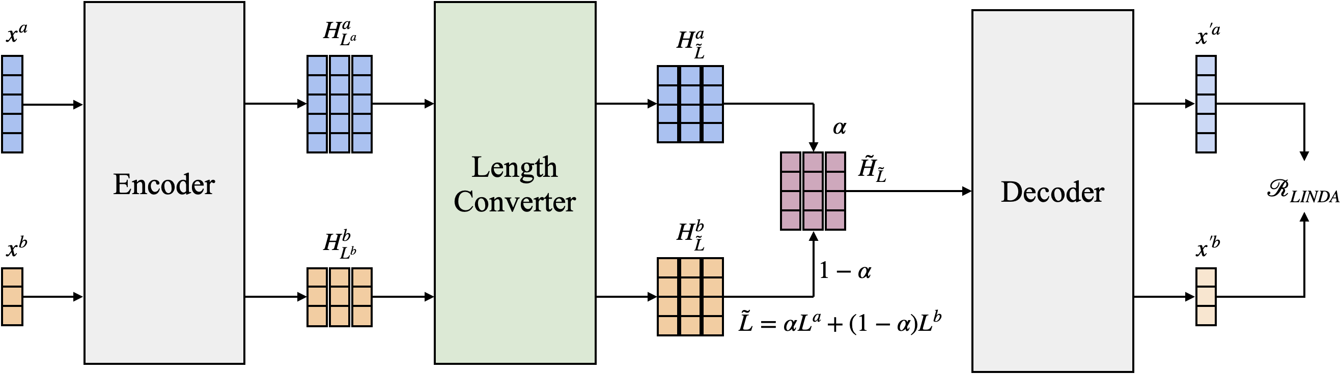
Figure 1: The overall architecture of our framework. Input texts $x^{a}$ and $x^{b}$ of which have possibly varying lengths are encoded and passed to the length converter to be transformed into representations with the interpolated matching length, $\tilde{L}$. $H_{L}^{a}$ and $H_{L}^{b}$, are interpolated into $\tilde{H}_{L}$ with the mixup ratio $\alpha$. The decoder is trained to reconstruct $\tilde{H}_{L}$ into $x^{a}$ and $x^{b}$ with the risk, $\mathcal{R}_{\mathrm{LINDA}}$. We show an example where $x^{a}$ and $x^{b}$ has length 5 and 3, respectively and the hidden dimension size is 3.

2.3 Non-Mixup Data Augmentation in NLP

Although we focus on mixup in this paper, data augmentation has been studied before however focusing on using a single training example at a time. One family of such approaches is a token-level replacement. Wei and Zou (2019a) suggests four simple data augmentation techniques, such as synonym replacement, random insertion, random swap, and random deletion, to boost text classification performance. Xie et al. (2019) substitutes the existing noise injection methods with data augmentation methods such as RandAugment Cubuk et al. (2019) or back-translation. All these methods are limited in that first, they cannot consider larger context when replacing an individual word, and second, replacement rules must be manually devised.

Another family consists of algorithms that rely on using a language model to produce augmentation. Wu et al. (2019) proposes conditional BERT contextual augmentation for labeled sentences using replacement-based methods. Anaby-Tavor et al. (2020) use GPT2 Radford et al. (2019) instead to synthesize examples for a given class. More recently, Kumar et al. (2020b) uses any pre-trained transformer Vaswani et al. (2017) based models for data augmentation. These augmentation strategies are highly specialized for a target classification task and often require finetuning with labeled examples. This makes them less suitable for low-resource settings in which there are by definition not enough labeled examples, to start with.

An existing approach that is perhaps closest to our proposal is self-supervised manifold-based data augmentation (SSMBA) by Ng et al. (2020a). SSMBA uses any masked language model as a denoising autoencoder which learns to perturb any given sequence along the data manifold. This enables SSMBA to produce realistic-looking augmented examples without resorting to any hand-crafted rules and to make highly non-trivial perturbation, beyond simple token replacement. It also does not require any labeled example.

Ng et al. (2020a) notice themselves such augmentation is nevertheless highly local. This implies that an alternative approach that makes non-local augmentation may result in a classifier that behaves better over the data manifold and achieves superior generalization and robustness. This is the goal of our proposal which we describe in the next section.

3 LINDA: Learning to Interpolate for Data Augmentation

In this section, we first define text interpolation (discrete sequence interpolation) and discuss desiderata that should be met. We then describe how we implement this notion of text interpolation using neural sequence modeling. We present a neural net architecture and a learning objective function used to train this neural network and show how to use a trained neural network for data augmentation.

3.1 Text Interpolation

We are given two sequences (text), $x^{a}=(x^{a}_{1},\ldots,x^{a}_{L^{a}})$ and $x^{b}=(x^{b}_{1},\ldots,x^{b}_{L^{b}})$. They are potentially of two different lengths, i.e., $L^{a}\neq L^{b}$, and each token is from a finite vocabulary, i.e., $x^{a}_{i}\in\Sigma$ and $x^{b}_{j}\in\Sigma$. With these two sequences, we define text interpolation as a procedure of drawing another sequence from the following conditional distribution:

$$p(y|x^{a},x^{b},\alpha)=\prod_{t=1}^{L^{y}}p(y_{t}|y_{<t},x^{a},x^{b},\alpha),$$ (2)

where $\alpha\in[0,1]$ is a mixup ratio, and $L^{y}$ is the length of an interpolated text $y$.

In order for sampling from this distribution to be text interpolation, four conditions must be met. Let us describe them informally first. First, when $\alpha$ is closer to $0$, a sample drawn from this distribution should be more similar to $x^{a}$. When $\alpha$ is closer to $1$, it should be more similar to $x^{b}$. It is however important that any sample must be similar to both $x^{a}$ and $x^{b}$. Finally, this distribution must be smooth in that we should be able to draw samples that are neither $x^{a}$ and $x^{b}$. If the final two conditions were not met, we would not call it “inter”polation.

Slightly more formally, these conditions translate to the following statements. First, (Condition 1) $p(x^{a}|x^{a},x^{b},\alpha)>p(x^{b}|x^{a},x^{b},\alpha)$ when $\alpha<0.5$. Similarly, (Condition 2) $p(x^{a}|x^{a},x^{b},\alpha)<p(x^{b}|x^{a},x^{b},\alpha)$ when $\alpha>0.5$. The third condition can be stated as (Condition 3) $p(x^{a}|x^{a},x^{b},\alpha)\gg 0$ and $p(x^{b}|x^{a},x^{b},\alpha)\gg 0$, although this does not fully capture the notion of similarity between an interpolated sample and either of $x^{a}$ or $x^{b}$. We rely on parametrization and regularization to capture this aspect of similarity. The final condition translates to (Condition 4) $p(x^{a}|x^{a},x^{b},\alpha)+p(x^{b}|x^{a},x^{b},\alpha)\ll 1$.

In the rest of this section, we describe how to parametrize this interpolation distribution with a deep neural network and train it to satisfy these conditions, for us to build the first learning-based text interpolation approach.

3.2 Parametrization

As shown in Figure 1, LINDA uses an encoder-decoder architecture to parametrize the interpolation distribution in Eq. (2), resembling sequence-to-sequence learning (Sutskever et al., 2014; Cho et al., 2014). The encoder takes the inputs respectively and delivers the encoded examples to the length converter, where each encoded example is converted to the same length. Matching length representations of the inputs are then interpolated with $\alpha$. The decoder takes the interpolated representation and reconstructs the original inputs $x^{a}$ and $x^{b}$ proportionally according to the given $\alpha$ value.

Encoder

We assume the input is a sequence of discrete tokens, $x=(x_{1},...x_{L})\in\Sigma^{L}$, where $\Sigma$ is a finite set of unique tokens and $L$ may vary from one example to another. The encoder, which can be implemented as a bidirectional recurrent network (Bahdanau et al., 2014) or as a transformer (Vaswani et al., 2017), reads each of the input pairs and outputs a set of vector representations; $H^{a}=\{h^{a}_{1},\ldots,h^{a}_{L^{a}}\}$ and $H^{b}=\{h^{b}_{1},\ldots,h^{b}_{L^{b}}\}$.

Length Converter

Unlike in images where inputs are downsampled to a matching dimension, the original lengths of the input sequences are preserved throughout the computation in NLP. To match the varying lengths, preserving the original length information, we adapt a location-based attention method proposed by Shu et al. (2020). First, we set the target length, $\tilde{L}$, as the interpolated value of $L^{a}$ and $L^{b}$:

$$\tilde{L}=\lceil\alpha L^{a}+(1-\alpha)L^{b}\rceil.$$ (3)

Each vector set is either down- or up-sampled to match the interpolated length $\tilde{L}$ which results in $\tilde{H}^{a}=\{\tilde{h}^{a}_{1},\ldots,\tilde{h}^{a}_{\tilde{L}}\}$ and $\tilde{H}^{b}=\{\tilde{h}^{b}_{1},\ldots,\tilde{h}^{b}_{\tilde{L}}\}$. Each $\tilde{h}$ is a weighted sum of the hidden vectors: $\tilde{h}_{j}=\sum_{k=1}^{L}w_{k}^{j}h_{k},$ where $w_{k}^{j}=e^{a_{k}^{j}}\big{/}\sum_{k^{\prime}=1}^{L}e^{a_{k^{\prime}}^{j}}$ and $a_{k}^{j}=-\frac{1}{2\sigma^{2}}(k-\frac{L}{\tilde{L}}j)^{2}$ with trainable $\sigma$. We finally compute the interpolated hidden vector set $\tilde{H}=\{\tilde{h}_{1},\ldots,\tilde{h}_{\tilde{L}}\}$ by $\tilde{h}_{i}=\alpha\tilde{h}^{a}_{i}+(1-\alpha)\tilde{h}^{b}_{i}.$

Decoder

The decoder, which can be also implemented as a recurrent network or a transformer with causal attention, takes $\tilde{H}$ as an input and models the conditional probability distribution of the original input sequences $x^{a}$ and $x^{b}$ accordingly to the mixup ratio $\alpha$. The decoder’s output is then the interpolation distribution $p(y|x^{a},x^{b},\alpha)$ in Eq. (2).

3.3 A Training Objective Function

We design a training objective and regularization strategy so that a trained model is encouraged to satisfy the four conditions laid out above and produces a text interpolation distribution.

A main objective.

We design a training objective function to impose the conditions laid out earlier in §3.1. The training objective function for LINDA is

$$\mathcal{R}_{\text{LINDA}}=-\frac{1}{N^{2}}\sum_{n,n^{\prime}=1}^{N}\int_{0}^{1}\alpha\log(p(x^{n}|x^{n},x^{n^{\prime}},\alpha)$$

$$\quad\quad\leavevmode\nobreak\ +(1-\alpha)\log(p(x^{n^{\prime}}|x^{n},x^{n^{\prime}},\alpha))\mathrm{d}\alpha,$$ (4)

where we assume there are $N$ training examples and consider all possible $\alpha$ values equally likely. Minimizing this objective function encourages LINDA to satisfy the first three conditions; a trained model will put a higher probability to one of the text pairs according to $\alpha$ and will refrain from putting any high probability to other sequences.

Because $\mathcal{R}_{\text{LINDA}}$ is computationally expensive, we resort to stochastic optimization in practice using a small minibatch of $M$ randomly-paired examples at a time with $\alpha\sim\mathcal{U}(0,1)$:

$$\tilde{\mathcal{R}}_{\text{LINDA}}=-\frac{1}{M}\sum_{m=1}^{M}\alpha\log p(x^{a,m}|x^{a,m},x^{b,m},\alpha^{m})$$

$$\quad+(1-\alpha)\log p(x^{b,m}|x^{a,m},x^{b,m},\alpha^{m}).$$ (5)

It is however not enough to minimize this objective function alone, as it does not prevent some of the degenerate solutions that violate the remaining conditions. In particular, the model may encode each possible input as a set of unique vectors such that the decoder is able to decode out both inputs $x^{a}$ and $x^{b}$ perfectly from the sum of these unique vector sets. When this happens, there is no meaningful interpolation between $x^{a}$ and $x^{b}$ learned by the model. That is, the model will put the entire probability mass divided into $x^{a}$ and $x^{b}$ but nothing else, violating the fourth condition. When this happens, linear interpolation of hidden states is meaningless and will not lead to meaningful interpolation in the text space, violating the third condition.

Regularization

In order to avoid the degenerate solution, we introduce three regularization techniques. First, inspired by the masked language modeling suggested in Devlin et al. (2019), we randomly apply the word-level masking to both inputs, $x^{a}$ and $x^{b}$. The goal is to force the model to preserve the contextual information from the original sentences. Each word of the input sentence is randomly masked using the masking probability, $p_{mask}$. The second one is to encourage each hidden vector out of the encoder to be close to the origin:

$$\mathcal{R}_{\text{LINDA}}^{\text{reg}}=\mathcal{R}_{\text{LINDA}}+\frac{\lambda}{M}\sum_{m=1}^{M}\sum_{i=1}^{L^{m}}\|h_{i}^{m}\|^{2},$$ (6)

where $\lambda\geq 0$ is a regularization strength. Finally, we add small, zero-mean Gaussian noise to each vector $h_{i}^{m}$ before interpolation during training. The combination of these two has an effect of tightly packing all training inputs, or their hidden vectors induced by the encoder, in a small ball centered at the origin. In doing so, interpolation between two points passes by similar, interpolatable inputs placed in the hidden space. This is similar to how variational autoencoders form their latent variable space (Kingma and Welling, 2013).

3.4 Augmentation

Once trained, the model can be used to interpolate any pair of sentences with an arbitrary choice of decoding strategy and distribution of $\alpha$. When we are dealing with a single-sentence classification, we draw random pairs of training examples with their labels as a minibatch, $((x_{m}^{a},y_{m}^{a}),(x_{m}^{b},y_{m}^{b}))$ along with a randomly drawn mixup ratio value ${\alpha}_{m}$. Then, based on the learned distribution, LINDA generates an interpolated version $\tilde{x_{m}}$ where we set the corresponding interpolated label to $\tilde{y_{m}}=(1-\alpha_{m})y_{m}^{a}+{\alpha_{m}}{y_{m}^{b}}$. In the case where the input consists of two sentences, we produce an interpolated sentence for each of these sentences separately. For instance, in the case of natural language inference (NLI) Rocktäschel et al. (2015), we interpolate the premise and hypothesis sentences separately and independently from each other and concatenate the interpolated premise and hypothesis to form an augmented training example.

4 LINDA: Training Details

We train LINDA once on a million sentence pairs randomly drawn from English Wikipedia and use it for all the experiments. We detail how we train this interpolation model in this section.

We base our interpolation model on a pre-trained BART released by Lewis et al. (2020). More specifically, we use BART-large. BART is a Transformer-based encoder-decoder model, pre-trained as a denoising autoencoder. We modify BART-large so that the encoder computes the hidden representations of two input sentences individually. These representations are up/downsampled to match the target interpolated length, after which they are linearly combined according to the mixing ratio. The decoder computes the interpolation distribution as in Eq. (2), in an autoregressive manner.

We train this model using the regularized reconstruction loss defined in Eq. (6). We uniformly sample the mixup ratio $\alpha\in[0,1]$ at random for each minibatch during training as well as for evaluation. We set the batch size to 8 and use Adam optimizer (Kingma and Ba, 2015) with a fixed learning rate of $1e^{-5}$. We use 8 GPUs (Tesla T4) for training. A word-level masking is adapt to input sentence with $p_{\mathrm{mask}}=0.1$. We set $\lambda=0.001$ and the standard deviation of Gaussian noise to $0.001$.

Once trained, we can produce an interpolated sentence from the model using any decoding strategy. We use beam search with beam size set to 4 in all the experiments.

5 Does LINDA Learn to Interpolate?

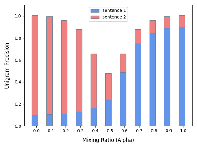
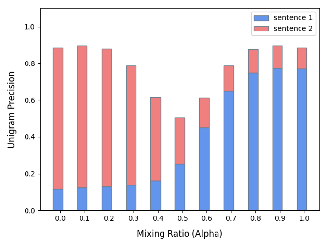
Figure 2: Average unigram precision of the interpolated sentences while varying the mixup ratio $\alpha$ in (top) Wikipedia and (bottom) TREC.

We first check whether LINDA preserves the contextual information of reference sentences proportionally to the mixup ratio $\alpha$, which is the key property of interpolation we have designed LINDA to exhibit. We investigate how much information from each of two original sentences is retained (measured in terms of unigram precision) while varying the mixup ratio $\alpha$. We expect a series of interpolated sentences to show a monotonically decreasing trend in unigram precision when computed against the first original sentence and the opposite trend against the second original sentence, as the mixup ratio moves from 1 to 0.

Figure 2 confirms our expectation and shows the monotonic trend. LINDA successfully reconstructs one of the original sentences with an extreme mixup ratio, with unigram precision scores close to $1$. As $\alpha$ nears $0.5$, the interpolated sentence deviates significantly from both of the input sentences, as anticipated. These interpolated sentences however continue to be well-formed, as we will show later for instance in Table 6 and Table 7 from Appendix. This implies that LINDA indeed interpolates sentences over a natural language manifold composed mostly of well-formed sentences only, as we expected and designed it for.

We observe a similar trend even when LINDA was used with non-Wikipedia sentences, as shown at the bottom of Figure 2 although overall unigram precision scores across the mixing ratios are generally a little bit lower than they were with Wikipedia.

In Table 1, we present four sample interpolations using four random pairs of validation examples from SST-2 Socher et al. (2013) and Yelp (see §6.1). As anticipated from the unigram precision score based analysis above, most of the interpolated sentences exhibit some mix of semantic and syntactic structures from both of the original sentences, according to the mixing ratio, as well-demonstrated in the first and third examples. The second example shows the LINDA’s capability of paraphrasing as well as using synonyms. In the final example, both of the inputs are not well-formed, unlike those sentences in Wikipedia, and LINDA fails to interpolate these two ill-formed sentences and resorts to producing a Wikipedia-style, well-formed sentence, which clearly lies on a natural language manifold, that has only a vague overlap with either of the input sentences. These examples provide us with evidence that LINDA has successfully learned to mix contents from two inputs, i.e., interpolate them, over a natural language manifold of well-formed sentences.

Mixup Ratio	Examples
0.50	Input 1	Relaxed in its perfect quiet pace and proud in its message
	Input 2	The plot is both contrived and cliched
	LINDA	The plot is both perfect and cliched in its message.
0.60	Input 1	Richly entertaining and suggestive of any number of metaphorical readings
	Input 2	The film is superficial and will probably be of interest primarily to its target audience
	LINDA	The film is very entertaining and will probably be of interest to many of its target audience regardless of its genre.
0.50	Input 1	Loved the Vegan menu! Glad to have so many options! The free margarita was really good also!
	Input 2	Service was awfully slow… food was just meh…. eventhough we get comp for drinks…. the whole experienced didnt make up for it..
	LINDA	Lincoln was very pleased with the menu… Glad to have so many options!…eventhough we got the free drinks for the whole team…it was really good..
0.54	Input 1	engaging , imaginative filmmaking in its nearly 2 1/2
	Input 2	the film has ( its ) moments , but
	LINDA	The film was released in the United States on October 2, 2019, and in Canada on October 3, 2019.

Table 1: Examples of interpolated sentences, generated by LINDA, and their original inputs on SST-2 and Yelp.

Overall, we find the observations in this section to be strong evidence supporting that the proposed approach indeed learns to interpolate between two sentences over a natural language manifold composed of well-formed sentences only. This is unlike existing interpolation approaches used for applying mixup to NLP, where interpolated sentences are almost never well-formed and cannot mix the original sentences in non-trivial ways.

Data Profile	Method	TREC-Coarse	TREC-Fine	SST-2	IMDB
Low	Vanilla	61.2$\pm$7.63 / 81.0$\pm$1.99	53.7$\pm$2.46 / 66.8$\pm$2.33	59.8$\pm$6.75 / 63.1$\pm$4.24	61.8$\pm$2.41 / 67.8$\pm$2.94
	EDA	57.0$\pm$6.54 / 72.0$\pm$4.64	54.7$\pm$1.73 / 66.5$\pm$4.19	62.3$\pm$3.18 / 60.5$\pm$2.81	62.5$\pm$3.00 / 69.0$\pm$3.04
	SSMBA	60.0$\pm$5.38 / 80.6$\pm$1.53	53.9$\pm$1.42 / 66.5$\pm$4.66	60.3$\pm$6.26 / 64.8$\pm$5.78	64.1$\pm$2.10 / 69.9$\pm$2.63
	Mixup	59.9$\pm$4.94 / 81.6$\pm$2.57	52.3$\pm$2.12 / 67.9$\pm$3.03	59.7$\pm$4.64 / 62.1$\pm$4.38	62.2$\pm$1.86 / 67.4$\pm$2.37
	LINDA	62.2$\pm$3.09 / 83.4$\pm$2.30	54.2$\pm$1.50 / 69.2$\pm$2.60	63.5$\pm$4.44 / 66.5$\pm$3.84	67.3$\pm$2.60 / 71.0$\pm$1.61
Full	Vanilla	97.2$\pm$0.36	87.9$\pm$1.05	92.3$\pm$0.06	89.2$\pm$0.59
	EDA	96.4$\pm$0.77	90.6$\pm$0.84	92.2$\pm$0.52	89.5$\pm$0.18
	SSMBA	96.9$\pm$0.41	90.2$\pm$0.71	92.3$\pm$0.38	89.2$\pm$0.17
	SSMBAsoft	97.3$\pm$0.23	88.3$\pm$0.54	92.3$\pm$0.35	89.4$\pm$0.13
	Mixup	97.5$\pm$0.30	86.4$\pm$1.23	92.4$\pm$0.41	89.1$\pm$0.18
	LINDA	97.6$\pm$0.36	91.6 $\pm$0.75	92.8$\pm$0.34	89.3 $\pm$0.18

Table 2: Comparison of classification accuracy (%) of BERT_BASE after fine-tuning with each data augmentation method on four different datasets under full and low resource (5-shot/10-shot) settings. All the results are reported as “mean(±std)” across 5 random runs. The best results are indicated in bold.

Method	RTE	QNLI	MNLI-m/m	ARclothing		Movie		Yelp
				ID	OOD	ID	OOD	ID	OOD
Vanilla	68.2$\pm$1.78	88.0$\pm$0.77	77.0$\pm$0.50 / 77.6 $\pm$0.46	73.1$\pm$2.85	73.0$\pm$2.86	90.8$\pm$0.33	84.8$\pm$0.74	66.0$\pm$0.88	65.4$\pm$1.49
EDA	65.6$\pm$2.22	86.6$\pm$0.70	76.4$\pm$0.27 / 77.1$\pm$0.39	72.6$\pm$2.86	72.6$\pm$2.79	90.8$\pm$0.35	84.8$\pm$0.88	64.9$\pm$0.97	64.8$\pm$1.26
SSMBA	66.8$\pm$2.18	87.6$\pm$0.58	76.4$\pm$1.18 / 77.3$\pm$0.51	72.6$\pm$2.85	72.8$\pm$2.70	90.8$\pm$0.27	84.7$\pm$0.79	65.7$\pm$1.13	65.3$\pm$1.00
SSMBAsoft	69.4$\pm$2.36	88.5$\pm$1.08	77.0$\pm$0.10 / 77.7$\pm$0.29	73.2$\pm$2.85	73.6$\pm$2.92	90.8$\pm$0.24	85.5$\pm$0.86	66.5$\pm$1.03	65.8$\pm$1.31
Mixup	70.9$\pm$0.94	87.6$\pm$1.13	76.8$\pm$0.22 / 77.6$\pm$0.31	72.9$\pm$2.77	72.9$\pm$2.80	90.7$\pm$0.30	83.9$\pm$1.71	65.6$\pm$0.88	65.2$\pm$1.20
LINDA	71.9$\pm$1.87	88.6$\pm$0.25	77.4$\pm$0.27 / 78.0$\pm$0.29	73.5$\pm$2.87	73.2$\pm$2.82	91.0$\pm$0.25	85.7$\pm$0.86	66.2$\pm$1.19	65.6$\pm$1.20

Table 3: Average evaluation accuracy (%) of BERT_BASE across 5 runs. First three columns show accuracy in NLI datasets and the following three columns show accuracy in ID and OOD settings with the AR_clothing, Movie, and Yelp datasets. See Appendix D for accuracy in each category. All the results are reported as “mean(±std)” across 5 random runs. The best results are indicated in bold.

6 LINDA for Data Augmentation

Encouraged by the promising interpolation results from the previous section, we conduct an extensive set of experiments to verify the effectiveness of LINDA for data augmentation in this section.

We run all experiments in this section by fine-tuning a pre-trained BERT-base Devlin et al. (2019) using Adam Kingma and Ba (2015) with a fixed learning rate of $3e^{-5}$. We use the batch size of 32 and train a model for 5 epochs when we use a full task dataset, and the batch size of 8 for 30 epochs in the case of low-resource settings. We report the average accuracy and standard deviation over five runs. For each training example, we produce one perturbed example from a data augmentation method so that the size of the augmented dataset matches that of the original training set. We test three different labeling strategies for LINDA and report the best accuracy. For further details, refer to Appendix C.

6.1 Downstream Tasks

We conduct experiments on seven datasets: TREC (coarse, fine) Li and Roth (2002), SST-2, IMDBMaas et al. (2011), RTE Wang et al. (2018a), MNLI Williams et al. (2018) and QNLI Rajpurkar et al. (2016). For each dataset, we create two versions of training scenarios; a full setting where the original training set is used, and a low-resource setting where only 5 or 10 randomly selected training examples per class are used. We also test LINDA on OOD generalization, by closely following the protocol from (Ng et al., 2020a). We use the Amazon Review Ni et al. (2019) and Yelp Review datasets as well as the Movies dataset created by combining SST-2 and IMDB. We train a model separately on each domain and evaluate it on all the domains. We report the in-domain and OOD accuracies. See Appendix B for more details.

6.2 Baselines

We compare LINDA against three existing augmentation methods. First, EDAWei and Zou (2019b) is a heuristic method that randomly performs synonym replacement, random insertion, random swap, and random deletion. Second, SSMBA Ng et al. (2020a) perturbs an input sentence by letting a masked language model reconstruct a randomly corrupted input sentence. For SSMBA, we report two different performances; one (SSMBA) where the label of an original input is used as it is, and the other (SSMBA_soft) where a predicted categorical distribution (soft label) by another classifier trained on an original, unaugmented dataset is used. Third, mixup Guo et al. (2019) mixes a pair of sentence at the sentence embedding level.

6.3 Result

In Table 2 we present the results on four text classification datasets for both full and low-resource settings. In the case of low-resource settings, LINDA outperforms all the other augmentation methods except for the 5-shot setting with the TREC-fine task, although the accuracies are all within standard deviations in this particular case. Because Ng et al. (2020a) reported low accuracies when predicted labels were used with a small number of training examples already, we do not test SSMBA_soft in the low-resource settings. Similarly in the full setting, LINDA outperforms all the other methods on all datasets except for IMDB, although the accuracies are all within two standard deviations. This demonstrates the effectiveness of the proposed approach regardless of the availability of labeled examples.

In the first three columns of Table 3, we report accuracies on the NLI datasets; RTE, QNLI and MNLI ans show that LINDA outperforms other data augmentation methods on all of the three datasets. LINDA improves the evaluation accuracy by 5.4% on RTE, 0.7% on QNLI, and 0.5% on MNLI when all the other augmentation methods, except for SSMBA_soft, degrade the baseline (Vanilla) performance.

We report the result from the OOD generalization experiments in the last three columns of Table 3. Although SSMBA_soft achieves the greatest improvement in OOD generalization over the vanilla approach in AR_clothing and Yelp, LINDA does not fail to show improvement over the baseline across all datasets in both in-domain and OOD settings. In agreement with Ng et al. (2020a), we could not observe any improvement with the other augmentation methods, EDA and Mixup, in this experiment.

7 Conclusion

Mixup, which was originally proposed for computer vision applications, has been adapted in recent years for the problems in NLP. To address the issues of arising from applying mixup to variable-length discrete sequences, existing efforts have largely relied on heuristics-based interpolation. In this paper, we take a step back and started by contemplating what it means to interpolate two sequences of different lengths and discrete tokens. We then come up with a set of conditions that should be satisfied by an interpolation operator on natural language sentences and proposed a neural net based interpolation scheme, called LINDA, that stochastically produces an interpolated sentence given a pair of input sentences and a mixing ratio.

We empirically show that LINDA is indeed able to interpolate two natural language sentences over a natural language manifold of well-formed sentences both quantitatively and qualitatively. We then test it for the original purpose of data augmentation by plugging it into mixup and testing it on nine different datasets. LINDA outperforms all the other data augmentation methods, including EDA and SSMBA, on most datasets and settings, and consistently outperforms non-augmentation baselines, which is not the case with the other augmentation methods.

Appendix A Interpolation on Different Domain

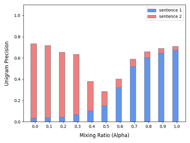
Figure 3: Average unigram precision score of the interpolated sentences with varying mixup ratio values in the SST-2 dataset.

Figure 3 shows the average unigram precision score of the interpolated sentences with respect to the mixup ratio, $\alpha$. We observe that the general trend is identical to the average unigram precision score measured in the Wikipedia corpus and TREC, as presented in Figure 2.

Appendix B Details of Downstream Datasets

Dataset	Task	Label	Train
TRECcoarse	Classification	6	5.5k
TRECfine	Classification	47	5.5k
SST-2	Sentiment	2	67k
IMDB	Sentiment	2	46k
RTE	NLI	2	2.5k
MNLI	NLI	3	25k†
QNLI	NLI	2	25k†
ARclothing	Ratings	5	25k†
Yelp	Ratings	5	25k†

Table 4: Dataset summary statistics. C, S, OOD, and, NLI in the task column represents classification, sentiment analysis, out-of-distribution, and natural language inference respectively. Training sets marked with a $\dagger$ are sampled randomly from a larger dataset.

Dataset		#
TRECcoarse		5.5k / 500
TRECfine		5.5k / 500
SST-2		67k / 872
IMDB		25k / 25k
RTE		2.5k / 3k
MNLI		2.5k / 9.7k
QNLI		2.5k / 5.5k
ARclothing	Clothing	25k / 2k
	Women	25k / 2k
	Men	25k/ 2k
	Baby	25k/ 2k
	Shoes	25k / 2k
YELP	American	25k / 2k
	Chinese	25k / 2k
	Italian	25k / 2k
	Japanese	25k / 2k

Table 5: Summary of which split of dataset is used to report the performance on downstream datasets. Column # indicates the number of samples in the data split as either in (train/validation) or in (train/test) based on the split used to report the performance with.

We present the details of downstream datasets in Table 4. For experiments, we report accuracy using the official test set on TREC, IMDB, AR and YELP. For those where the label for the official test set is not available, SST-2, RTE, MNLI and QNLI, we use the validation set as the test set. Further details are shown in Table 5. SST-2 and RTE are from the GLUE dataset Wang et al. (2018b). We report the number of the samples in each split in the (train/validation) format. Rows for TREC and IMDB are reported in the (train/test) format.

For ID and OOD experiments, we use three different datasets; AR_clothing, Yelp, Movies. AR_clothing consists with five clothing categories: Clothes, Women clothing, Men Clothing, Baby Clothing, Shoes and Yelp, following the preprocessing in Hendrycks et al. (2020), with four groups of food types: American, Chinese, Italian, and Japanese. For both datasets, we sample 25,000 reviews for each category and the model predicts a review’s 1 to 5 star rating. Movie dataset is consists with SST-2 and IMDB. We train the model separately on each domain, then evaluate on all domains to report the average in-domain and OOD performance across 5 runs.

Appendix C Label Generation for LINDA

C.1 Choice of the Label Generation

Label	$T$	TREC-Coarse	TREC-Fine	SST-2	IMDB	RTE	QNLI	MNLI-(m/mm)
Interpolated	1	97.6$\pm$0.36	91.4$\pm$0.26	92.3$\pm$0.43	89.2$\pm$0.15	66.1$\pm$3.8	88.0$\pm$0.4	77.0$\pm$0.3/77.1$\pm$0.2
Interpolated	0.5	97.4$\pm$0.21	91.6$\pm$0.75	92.2$\pm$0.37	89.3$\pm$0.22	66.8$\pm$1.4	87.4$\pm$0.7	76.2$\pm$0.4/77.1$\pm$0.4
predicted	-	97.4$\pm$0.09	90.1$\pm$0.39	92.8$\pm$0.34	89.3$\pm$0.18	71.9$\pm$1.9	88.6$\pm$0.2	77.4$\pm$0.3/78.0$\pm$0.3

Table 6: Effect of using the different label generation

For the full dataset setting, shown in Table 2, evaluation accuracy of LINDA is reported with different labeling method for each dataset. Note that we only report accuracy with the interpolated labels in the low-resources settings since (Ng et al., 2020b) has already reported that with a small amount of training examples, using the psuedo labeling show low accuracies. Using the interpolated labels for TREC-coarse and TREC-Fine shows the best performances in the full dataset setting. However, for IMDB and SST-2, utilizing the predicted soft label shows the best performance for the full setting experiment.

For NLI experiments, reported in Table 3, best performances for all three datasets are also with the predicted soft label. Lastly, for the ID and OOD experiments in Table 3, using the predicted soft label shows the best performance in AR_clothing and Yelp datasets across all domains (five different domains in AR_clothing and four different domains in Yelp). In Movie, using the interpolated labels explained in §3.4 shows the best result when training the model on IMDB and evaluating on SST-2. However, when training the model on SST-2 and evaluating on IMDB, using the predicted soft label shows the best result.

C.2 Effect of Label Sharpening

Although we apply linear interpolation in LINDA, we observed that unigram precision score of interpolated sentence is on the side of the larger $\alpha$ value well Figure 2 in §5. Based on this observation, we investigate the effect of sharpening our label $\tilde{y}$ by applying the sharpening with temperature $T$ Heaton (2017). Denote $\tilde{y}$ is soft label of a class distributions $\tilde{y_{i}}$ and sharpening operation is defined as operation

$$Sharpen(\tilde{y_{m}},T)=\tilde{y_{i}}^{1/T}/\sum_{i=1}^{L}exp(\tilde{y_{i}}^{1/T}),$$ (7)

When $T$ equals 1, the label does not change and as $T$ gets closer to 0, $Sharpen(\tilde{y},T)$ approaches to a hard label. We show the effect of using sharpened labels in Table 6.

C.3 Effect of the predicted Label

As our approach is under the unsupervised learning scheme, where only contextual information is considered, interpolated labels suggested in 3.4 have risk of being mismatched with the correct label. Therefore, we investigate using the predicted label which is evaluated with the model taught with the original training data, which we call teacher, to makes the model to be susceptible to the damaged label issue. Once the teacher model is trained on the original set of unaugmented data, we evaluate augmented samples and replace the label information $\tilde{y}$ with the output probability of a trained teacher model. In Table 6, we show the difference in accuracy when the interpolated label is used versus when the predicted label is used. It shows that using the predicted label significantly improves the performance in SST-2 and NLI datasets, despite of using the interpolated label even hurting the performance.

Appendix D ID and OOD Results over All Domains

Table 3 in §6.3 shows the average ID and OOD accuracy (%) over all categories. However, unlike the Movie dataset, where it consists of only two domains; SST-2 and IMDB, AR_clothing and Yelp datasets consist of multiple domains. AR_clothing consists with five clothing categories: Clothes, Women clothing, Men Clothing, Baby Clothing, Shoes and Yelp, following the preprocessing in Hendrycks et al. (2020), with four groups of food types: American, Chinese, Italian, and Japanese. We report accuracy (%) over all categories along with standard deviation values over 5 random runs in the AR_clothing and Yelp datasets in Table 8 and Table 9.

Appendix E Effect of the Mixup Ratio with Wikipedia Sentences

We present an example of the interpolated sentences from Wikipedia sentences with the varying values of $alpha$ in Table 7. Two reference sentences are randomly drawn from English Wikipedia corpus. As $alpha$ gets closer to 1, the interpolated sentence resembles the sentence 1 more and as $alpha$ gets closer to 0, it resembles the sentence 2 more. Moreover, we see that LINDA is capable of generating sentences using tokens that have never appeared in the reference sentences as well. This capability of LINDA comes from leveraging the power of pre-trained generation model, BART, on the vast amount of English Wikipedia sentences with the reconstruction loss.

Sentence 1	Sentence 2
Henry tried, with little success, to reacquire the property Richard had sold, and had to live modestly as a gentle man, never formally taking title to the earldom	Kobilje Creek, a left tributary of the Ledava River, flows through it.

$\alpha$	Generated Sentences
0.1	Kobilje Creek, a left tributary of the Ledava River, flows through it.
0.2	Kobilje Creek, a left tributary of the Ledava River, flows through it to the north.
0.3	Kobilje Creek, a left tributary of the River Ledava, flows through it, as does a small river.
0.4	Kobilje, a small creek, left the tributary of the Ledava River, and it flows through the town.
0.5	Kenny, with a little help from his father, was able to take over the family business, which had been run by his mother.
0.6	Henry tried, with little success, to reacquaint himself with the property, and had to live as a modest earl.
0.7	Henry tried, with little success, to reacquaint himself wit h the property, and had to live as a modest gentleman, never formally taking part in the title.
0.8	Henry tried, with little success, to reacquaint himself with the property, and had to live as a modest gentleman, never formally taking title to the earldom
0.9	Henry tried, with little success, to reacquire the property Richard had sold, and had to live modestly as a gentleman, never formally taking title to the title.

Table 7: Example of a series of interpolated sentences by adjusting the value of $alpha$ given two input sentences.

Vanilla Clothing Women Men Baby Shoes Clothing 72.1$\pm$0.48 - - - - Women 69.2$\pm$0.73 69.6$\pm$0.40 - - - Men 72.4$\pm$0.64 72.0$\pm$1.15 72.7$\pm$0.50 - - Baby 77.1$\pm$0.35 76.4$\pm$0.92 77.5$\pm$1.00 78.0$\pm$0.44 - Shoes 71.6$\pm$0.75 71.3$\pm$0.44 72.4$\pm$0.82 70.5$\pm$0.51 73.2$\pm$0.61	EDA Clothing Women Men Baby Shoes Clothing 71.9$\pm$0.30 - - - - Women 68.1$\pm$0.33 69.5$\pm$0.58 - - - Men 71.6$\pm$0.37 71.5$\pm$1.04 71.8$\pm$0.29 - - Baby 76.8$\pm$0.42 76.2$\pm$0.28 76.1$\pm$0.30 77.9$\pm$0.44 - Shoes 71.6$\pm$0.72 72.0$\pm$0.69 71.3$\pm$0.57 70.4$\pm$0.82 71.9$\pm$0.23
SSMBA Clothing Women Men Baby Shoes Clothing 71.7$\pm$0.24 - - - - Women 68.9$\pm$0.65 69.2$\pm$0.22 - - - Men 72.3$\pm$0.65 71.1$\pm$0.73 71.8$\pm$0.26 - - Baby 76.7$\pm$0.75 76.3$\pm$0.56 76.5$\pm$0.64 77.6$\pm$0.26 - Shoes 72.1$\pm$0.75 72.1$\pm$0.62 71.8$\pm$0.75 70.4$\pm$0.58 72.8$\pm$0.34	SSMBAsoft Clothing Women Men Baby Shoes Clothing 72.9$\pm$0.41 - - - - Women 69.3$\pm$0.19 70.0$\pm$0.35 - - - Men 72.6$\pm$0.66 72.6$\pm$0.58 72.8$\pm$0.40 - - Baby 77.9$\pm$0.30 77.6$\pm$0.66 77.4$\pm$0.71 78.4$\pm$0.75 - Shoes 72.5$\pm$0.52 72.6$\pm$0.54 72.2$\pm$0.79 70.9$\pm$0.64 72.7$\pm$0.58
Mixup Clothing Women Men Baby Shoes Clothing 72.0$\pm$0.42 - - - - Women 68.3$\pm$0.51 69.6$\pm$0.25 - - - Men 71.7$\pm$0.41 72.3$\pm$0.50 72.2$\pm$0.30 - - Baby 76.3$\pm$1.09 76.7$\pm$0.65 76.7$\pm$0.74 77.8$\pm$0.25 - Shoes 71.6$\pm$0.72 72.1$\pm$0.50 72.0$\pm$0.66 70.3$\pm$0.63 73.0$\pm$0.46	LINDA Clothing Women Men Baby Shoes Clothing 71.4$\pm$0.34 - - - - Women 68.4$\pm$0.58 69.2$\pm$0.46 - - - Men 72.4$\pm$0.48 71.6$\pm$0.65 72.4$\pm$0.33 - - Baby 77.6$\pm$0.26 77.0$\pm$1.16 76.4$\pm$0.92 77.7$\pm$0.50 - Shoes 72.0 $\pm$0.49 71.9$\pm$0.67 71.6$\pm$0.69 70.4$\pm$0.82 73.1$\pm$0.19
LINDAsoft Clothing Women Men Baby Shoes Clothing 72.8$\pm$0.27 - - - - Women 69.4$\pm$0.59 69.9$\pm$0.43 - - - Men 71.7$\pm$0.31 72.6$\pm$0.39 72.7$\pm$0.44 - - Baby 77.3$\pm$0.39 77.2$\pm$0.18 77.0$\pm$0.12 78.5$\pm$0.43 - Shoes 72.5$\pm$0.46 71.7$\pm$0.64 72.0$\pm$0.26 70.4$\pm$0.82 73.4$\pm$0.61

Table 8: Accuracy (%) of BERT_BASE in the AR_clothing dataset. Each column represents the category where a model is trained with and each row represents the category where a model is evaluated on. All the results are reported as “mean(±std)” across 5 random runs.

Vanilla American Chinese Italian Japanese American 66.2 $\pm$0.49 - - - Chinese 63.0$\pm$1.18 64.7$\pm$0.58 - - Italian 66.8$\pm$0.52 65.7$\pm$0.40 66.4$\pm$0.34 - Japanese 65.5$\pm$1.34 66.4$\pm$0.99 64.9$\pm$0.48 66.6$\pm$0.52	EDA American Chinese Italian Japanese American 65.3$\pm$0.20 - - - Chinese 63.1$\pm$072 63.4$\pm$0.41 - - Italian 65.5$\pm$0.59 64.6$\pm$1.48 65.2$\pm$0.75 - Japanese 65.3$\pm$0.71 65.8$\pm$0.82 64.3$\pm$1.63 65.6 $\pm$0.38
SSMBA American Chinese Italian Japanese American 65.8$\pm$0.93 - - - Chinese 64.4$\pm$0.80 64.1$\pm$0.16 - - Italian 65.5$\pm$1.20 65.2$\pm$0.45 66.4$\pm$0.50 - Japanese 65.3$\pm$0.39 66.3$\pm$0.82 65.2$\pm$1.31 66.6$\pm$0.29	SSMBAsoft American Chinese Italian Japanese American 66.6$\pm$0.69 - - - Chinese 63.9$\pm$1.02 65.1$\pm$0.53 - - Italian 66.5$\pm$0.46 65.6$\pm$0.58 67.4$\pm$0.58 - Japanese 66.1$\pm$0.69 67.5$\pm$0.98 65.4$\pm$0.62 67.1$\pm$0.18
Mixup American Chinese Italian Japanese American 65.6$\pm$0.59 - - - Chinese 63.5$\pm$1.05 64.5$\pm$0.58 - - Italian 66.0$\pm$1.17 65.1$\pm$0.63 66.3$\pm$0.52 - Japanese 65.9$\pm$0.72 66.0$\pm$0.67 65.3$\pm$0.93 66.2$\pm$0.38	LINDA American Chinese Italian Japanese American 65.5$\pm$0.75 - - - Chinese 63.7$\pm$0.76 64.0$\pm$0.37 - - Italian 66.3$\pm$0.69 65.3$\pm$0.98 66.1$\pm$0.21 - Japanese 65.8$\pm$0.61 65.5$\pm$1.02 64.3$\pm$1.07 66.7$\pm$0.21
LINDAsoft American Chinese Italian Japanese American 66.2$\pm$0.72 - - - Chinese 64.2$\pm$0.42 64.7$\pm$0.51 - - Italian 66.2$\pm$0.86 65.9$\pm$0.44 67.3$\pm$0.98 - Japanese 65.7$\pm$0.56 67.0$\pm$0.75 64.6$\pm$1.35 66.8$\pm$0.45

Table 9: Accuracy (%) of BERT_BASE in the Yelp dataset. Each column represents the category where a model is trained with and each row represents the category where a model is evaluated on. All the results are reported as “mean(±std)” across 5 random runs.

References

- Anaby-Tavor et al. (2020) Ateret Anaby-Tavor, Boaz Carmeli, Esther Goldbraich, Amir Kantor, George Kour, Segev Shlomov, Naama Tepper, and Naama Zwerdling. 2020. Do not have enough data? deep learning to the rescue! In Proceedings of the AAAI Conference on Artificial Intelligence.
- Bahdanau et al. (2014) Dzmitry Bahdanau, Kyunghyun Cho, and Yoshua Bengio. 2014. Neural machine translation by jointly learning to align and translate. arXiv preprint arXiv:1409.0473.
- Chen et al. (2020) Jiaao Chen, Zichao Yang, and Diyi Yang. 2020. Mixtext: Linguistically-informed interpolation of hidden space for semi-supervised text classification. arXiv preprint arXiv:2004.12239.
- Cho et al. (2014) Kyunghyun Cho, Bart Van Merriënboer, Caglar Gulcehre, Dzmitry Bahdanau, Fethi Bougares, Holger Schwenk, and Yoshua Bengio. 2014. Learning phrase representations using rnn encoder-decoder for statistical machine translation. arXiv preprint arXiv:1406.1078.
- Cubuk et al. (2019) Ekin D Cubuk, Barret Zoph, Jonathon Shlens, and Quoc V Le. 2019. Randaugment: Practical data augmentation with no separate search. arXiv preprint arXiv:1909.13719, 2(4):7.
- Devlin et al. (2019) Jacob Devlin, Ming-Wei Chang, Kenton Lee, and Kristina Toutanova. 2019. BERT: Pre-training of deep bidirectional transformers for language understanding. In Proceedings of the 2019 Conference of the North American Chapter of the Association for Computational Linguistics: Human Language Technologies, Volume 1 (Long and Short Papers), pages 4171–4186, Minneapolis, Minnesota. Association for Computational Linguistics.
- Edunov et al. (2018) Sergey Edunov, Myle Ott, Michael Auli, and David Grangier. 2018. Understanding back-translation at scale. In Proceedings of the 2018 Conference on Empirical Methods in Natural Language Processing, pages 489–500, Brussels, Belgium. Association for Computational Linguistics.
- Guo et al. (2019) Hongyu Guo, Yongyi Mao, and Richong Zhang. 2019. Augmenting data with mixup for sentence classification: An empirical study. arXiv preprint arXiv:1905.08941.
- Heaton (2017) Jeff Heaton. 2017. Ian goodfellow, yoshua bengio, and aaron courville: Deep learning. Genetic Programming and Evolvable Machines, 19:305–307.
- Hendrycks et al. (2020) Dan Hendrycks, Xiaoyuan Liu, Eric Wallace, Adam Dziedzic, Rishabh Krishnan, and Dawn Song. 2020. Pretrained transformers improve out-of-distribution robustness. In Proceedings of the 58th Annual Meeting of the Association for Computational Linguistics, pages 2744–2751, Online. Association for Computational Linguistics.
- Kingma and Ba (2015) Diederik P. Kingma and Jimmy Ba. 2015. Adam: A method for stochastic optimization. CoRR, abs/1412.6980.
- Kingma and Welling (2013) Diederik P Kingma and Max Welling. 2013. Auto-encoding variational bayes. arXiv preprint arXiv:1312.6114.
- Kumar et al. (2020a) Amit Kumar, Rupjyoti Baruah, Rajesh Kumar Mundotiya, and Anil Kumar Singh. 2020a. Transformer-based neural machine translation system for Hindi – Marathi: WMT20 shared task. In Proceedings of the Fifth Conference on Machine Translation, pages 393–395, Online. Association for Computational Linguistics.
- Kumar et al. (2020b) Varun Kumar, Ashutosh Choudhary, and Eunah Cho. 2020b. Data augmentation using pre-trained transformer models. arXiv preprint arXiv:2003.02245.
- Lewis et al. (2020) Mike Lewis, Yinhan Liu, Naman Goyal, Marjan Ghazvininejad, Abdelrahman Mohamed, Omer Levy, Veselin Stoyanov, and Luke Zettlemoyer. 2020. BART: Denoising sequence-to-sequence pre-training for natural language generation, translation, and comprehension. In Proceedings of the 58th Annual Meeting of the Association for Computational Linguistics, pages 7871–7880, Online. Association for Computational Linguistics.
- Li and Roth (2002) Xin Li and Dan Roth. 2002. Learning question classifiers. In COLING 2002: The 19th International Conference on Computational Linguistics.
- Lim et al. (2019) Sungbin Lim, Ildoo Kim, Taesup Kim, Chiheon Kim, and Sungwoon Kim. 2019. Fast autoaugment. In NeurIPS.
- Maas et al. (2011) Andrew L. Maas, Raymond E. Daly, Peter T. Pham, Dan Huang, A. Ng, and Christopher Potts. 2011. Learning word vectors for sentiment analysis. In ACL.
- Ng et al. (2020a) Nathan Ng, Kyunghyun Cho, and Marzyeh Ghassemi. 2020a. Ssmba: Self-supervised manifold based data augmentation for improving out-of-domain robustness. arXiv preprint arXiv:2009.10195.
- Ng et al. (2020b) Nathan Ng, Kyunghyun Cho, and Marzyeh Ghassemi. 2020b. SSMBA: Self-supervised manifold based data augmentation for improving out-of-domain robustness. In Proceedings of the 2020 Conference on Empirical Methods in Natural Language Processing (EMNLP), pages 1268–1283, Online. Association for Computational Linguistics.
- Ni et al. (2019) Jianmo Ni, Jiacheng Li, and Julian McAuley. 2019. Justifying recommendations using distantly-labeled reviews and fine-grained aspects. In EMNLP.
- Radford et al. (2019) Alec Radford, Jeffrey Wu, Rewon Child, David Luan, Dario Amodei, Ilya Sutskever, et al. 2019. Language models are unsupervised multitask learners. OpenAI blog, 1(8):9.
- Rajpurkar et al. (2016) Pranav Rajpurkar, Jian Zhang, Konstantin Lopyrev, and Percy Liang. 2016. Squad: 100,000+ questions for machine comprehension of text. In EMNLP.
- Rocktäschel et al. (2015) Tim Rocktäschel, Edward Grefenstette, Karl Moritz Hermann, Tomáš Kočiskỳ, and Phil Blunsom. 2015. Reasoning about entailment with neural attention. arXiv preprint arXiv:1509.06664.
- Sennrich et al. (2015) Rico Sennrich, Barry Haddow, and Alexandra Birch. 2015. Improving neural machine translation models with monolingual data. arXiv preprint arXiv:1511.06709.
- Shu et al. (2020) Raphael Shu, Jason Lee, Hideki Nakayama, and Kyunghyun Cho. 2020. Latent-variable non-autoregressive neural machine translation with deterministic inference using a delta posterior. Proceedings of the AAAI Conference on Artificial Intelligence, 34(05):8846–8853.
- Socher et al. (2013) Richard Socher, Alex Perelygin, Jean Wu, Jason Chuang, Christopher D. Manning, A. Ng, and Christopher Potts. 2013. Recursive deep models for semantic compositionality over a sentiment treebank. In EMNLP.
- Sun et al. (2020) Lichao Sun, Congying Xia, Wenpeng Yin, Tingting Liang, Philip S. Yu, and Lifang He. 2020. Mixup-transformer: Dynamic data augmentation for nlp tasks. In COLING.
- Sutskever et al. (2014) Ilya Sutskever, Oriol Vinyals, and Quoc V Le. 2014. Sequence to sequence learning with neural networks. Advances in neural information processing systems, 27:3104–3112.
- Vaswani et al. (2017) Ashish Vaswani, Noam Shazeer, Niki Parmar, Jakob Uszkoreit, Llion Jones, Aidan N Gomez, Łukasz Kaiser, and Illia Polosukhin. 2017. Attention is all you need. In Advances in neural information processing systems, pages 5998–6008.
- Verma et al. (2019) Vikas Verma, Alex Lamb, Christopher Beckham, Amir Najafi, Ioannis Mitliagkas, David Lopez-Paz, and Yoshua Bengio. 2019. Manifold mixup: Better representations by interpolating hidden states. In International Conference on Machine Learning, pages 6438–6447. PMLR.
- Wang et al. (2018a) Alex Wang, Amanpreet Singh, Julian Michael, Felix Hill, Omer Levy, and Samuel R. Bowman. 2018a. Glue: A multi-task benchmark and analysis platform for natural language understanding. ArXiv, abs/1804.07461.
- Wang et al. (2018b) Alex Wang, Amanpreet Singh, Julian Michael, Felix Hill, Omer Levy, and Samuel R Bowman. 2018b. Glue: A multi-task benchmark and analysis platform for natural language understanding. arXiv preprint arXiv:1804.07461.
- Wei and Zou (2019a) Jason Wei and Kai Zou. 2019a. Eda: Easy data augmentation techniques for boosting performance on text classification tasks. arXiv preprint arXiv:1901.11196.
- Wei and Zou (2019b) Jason Wei and Kai Zou. 2019b. EDA: Easy data augmentation techniques for boosting performance on text classification tasks. In Proceedings of the 2019 Conference on Empirical Methods in Natural Language Processing and the 9th International Joint Conference on Natural Language Processing (EMNLP-IJCNLP), pages 6382–6388, Hong Kong, China. Association for Computational Linguistics.
- Williams et al. (2018) Adina Williams, Nikita Nangia, and Samuel Bowman. 2018. A broad-coverage challenge corpus for sentence understanding through inference. In Proceedings of the 2018 Conference of the North American Chapter of the Association for Computational Linguistics: Human Language Technologies, Volume 1 (Long Papers), pages 1112–1122, New Orleans, Louisiana. Association for Computational Linguistics.
- Wu et al. (2019) Xing Wu, Shangwen Lv, Liangjun Zang, Jizhong Han, and Songlin Hu. 2019. Conditional bert contextual augmentation. In International Conference on Computational Science, pages 84–95. Springer.
- Xie et al. (2019) Qizhe Xie, Zihang Dai, Eduard Hovy, Minh-Thang Luong, and Quoc V Le. 2019. Unsupervised data augmentation for consistency training. arXiv preprint arXiv:1904.12848.
- Yi et al. (2021) Mingyang Yi, Lu Hou, Lifeng Shang, Xin Jiang, Qun Liu, and Zhi-Ming Ma. 2021. Reweighting augmented samples by minimizing the maximal expected loss. ArXiv, abs/2103.08933.
- Yoon et al. (2021) Soyoung Yoon, Gyuwan Kim, and Kyumin Park. 2021. Ssmix: Saliency-based span mixup for text classification. ArXiv, abs/2106.08062.
- Zhang et al. (2017) Hongyi Zhang, Moustapha Cisse, Yann N Dauphin, and David Lopez-Paz. 2017. mixup: Beyond empirical risk minimization. arXiv preprint arXiv:1710.09412.
- Zhao and Cho (2019) Jake Zhao and Kyunghyun Cho. 2019. Retrieval-augmented convolutional neural networks against adversarial examples. In Proceedings of the IEEE Conference on Computer Vision and Pattern Recognition, pages 11563–11571.