Transformer Uncertainty Estimation with Hierarchical Stochastic Attention

Abstract

Transformers are state-of-the-art in a wide range of NLP tasks and have also been applied to many real-world products. Understanding the reliability and certainty of transformer model predictions is crucial for building trustable machine learning applications, e.g., medical diagnosis. Although many recent transformer extensions have been proposed, the study of the uncertainty estimation of transformer models is under-explored. In this work, we propose a novel way to enable transformers to have the capability of uncertainty estimation and, meanwhile, retain the original predictive performance. This is achieved by learning a hierarchical stochastic self-attention that attends to values and a set of learnable centroids, respectively. Then new attention heads are formed with a mixture of sampled centroids using the Gumbel-Softmax trick. We theoretically show that the self-attention approximation by sampling from a Gumbel distribution is upper bounded. We empirically evaluate our model on two text classification tasks with both in-domain (ID) and out-of-domain (OOD) datasets. The experimental results demonstrate that our approach: (1) achieves the best predictive performance and uncertainty trade-off among compared methods; (2) exhibits very competitive (in most cases, improved) predictive performance on ID datasets; (3) is on par with Monte Carlo dropout and ensemble methods in uncertainty estimation on OOD datasets.

1 INTRODUCTION

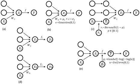
Figure 1: The methods of uncertainty estimation. (a) Deterministic neural network outputs a single-point prediction; (b) Bayesian neural network captures uncertainty via sampling from a Gaussian distribution; (c) Variational dropout captures uncertainty via sampling dropout masks from a Bernoulli distribution; (d) Ensemble captures uncertainty by combining multiple independently trained deterministic models with different random seeds; (e) Gumbel-Softmax trick for uncertainty estimation, the randomness comes from the sampling categorical distribution from a Gumbel.

Uncertainty estimation and quantification are important tools for building trustworthy and reliable machine learning systems (Lin, Engel, and Eslinger 2012; Kabir et al. 2018; Riedmaier et al. 2021). Particularly, when such machine-learned systems are applied to make predictions that involve important decisions, e.g., medical diagnosis (Ghoshal and Tucker 2020), financial planning and decision-making  (Baker et al. 2020; Oh and Hong 2021), and autonomous driving (Hoel, Wolff, and Laine 2020). The recent development of neural networks has shown excellent predictive performance in many domains. Among those, transformers, including the vanilla transformer (Vaswani et al. 2017) and its variants such as BERT (Devlin et al. 2019; Wang et al. 2020) are the representative state-of-the-art type of neural architectures that have shown remarkable performance on various recent Natural Language Processing (NLP) (Gillioz et al. 2020) and Information Retrieval (IR) (Ren et al. 2021) tasks.

Although transformers excel in terms of predictive performance (Tetko et al. 2020; Han et al. 2021), they do not offer the opportunity for practitioners to inspect the model confidence due to their deterministic nature, i.e., incapability to assess if transformers are confident about their predictions. This influence is non-trivial because transformers are cutting-edge basic models for NLP. Thus, estimating the predictive uncertainty of transformers benefits a lot in terms of building and examining model reliability for the downstream tasks.

To estimate the uncertainty of neural models’ prediction, one common way is to inject stochasticity (e.g., noise or randomness) (Kabir et al. 2018; Gawlikowski et al. 2021). It enables models to output a predictive distribution, instead of a single-point prediction. Casting a deterministic transformer to be stochastic requires us to take the training and inference computational complexity into consideration, because uncertainty estimation usually relies on multiple forward runs. Therefore, directly adapting the aforementioned methods is not desired, given the huge amount of parameters and architectural complexity of transformers.

Figure 1 outlines deterministic transformer (Figure 1(a)) and the possible approaches (Figure 1(b-e) for making a stochastic transformer. BNN (Figure 1(b)) assumes the network weights follow a Gaussian or a mixture of Gaussian (Blundell et al. 2015), and tries to learn the weight distribution $(\mu,\sigma)$, instead of weight $W$ itself, with the help of re-parameterization trick (Kingma and Welling 2014). That means, BNN doubles the number of parameters. This is particularly challenging for a large network like a transformer, which has millions of parameters to be optimized. To alleviate this issue, MC dropout (Gal and Ghahramani 2016) (Figure 1(c)) uses dropout (Srivastava et al. 2014), concretely Bernoulli distributed random variables, to approximate the exact posterior distribution (Gal and Ghahramani 2016). However, MC dropout tends to give overconfident uncertainty estimation (Foong et al. 2019). Ensemble (Lakshminarayanan, Pritzel, and Blundell 2017)(Figure 1(d)) is an alternative way to model uncertainty by averaging $N$ independently trained models, which yields the computational overhead by $N$ times in model training.

Unlike models above, we propose a simple yet effective approach based on Gumbel-Softmax tricks or Concrete Dropout (Jang, Gu, and Poole 2017; Maddison, Mnih, and Teh 2017), which are independently found for continuous relaxation, to estimate uncertainty of transformers. First, we cast the deterministic attention distribution for values in each self-attention head to be stochastic. The attention is then sampled from a Gumbel-Softmax distribution, which controls the concentration over values. Second, we regularize the key heads in self-attention to attend to a set of learnable centroids. This is equivalent to performing clustering over keys (Vyas, Katharopoulos, and Fleuret 2020) or clustering hidden states in RNN (Wang and Niepert 2019; Wang, Lawrence, and Niepert 2021). Similar attention mechanism has been also used to allow the layers in the encoder and decoder attend to inputs in the Set Transformer (Lee et al. 2019) and to estimate attentive matrices in the Capsule networks (Ahmed and Torresani 2019). Third, each new key head will be formed with a mixture of Gumbel-Softmax sampled centroids. The stochasticity is injected by sampling from a Gumbel-Softmax distribution. This is different from BNN (sampling from Gaussian distribution), MC-dropout (sampling from Bernoulli distribution), Ensemble (the stochasticity comes from random seeds in model training). With this proposed mechanism, we approximate the vanilla transformer with a stochastic transformer based on a hierarchical stochastic self-attention, namely H-sto-Trans, which enables the sampling of attention distributions over values as well as over a set of learnable centroids.

Our work makes the following contributions:

• We propose a novel way to cast the self-attention in transformers to be stochastic, which enables transformer models to provide uncertainty information with predictions.

• We theoretically show that the proposed self-attention approximation is upper bounded, the key attention heads that are close in Euclidean distance have similar attention distribution over centroids.

• In two benchmark tasks for NLP, we empirically demonstrate that H-sto-Trans (1) achieves very competitive (in most cases, better) predictive performance on in-domain datasets; (2) is on par with baselines in uncertainty estimation on out-of-domain datasets; (3) learns a better predictive performance-uncertainty trade-off than compared baselines, i.e., high predictive performance and low uncertainty on in-domain datasets, high predictive performance and high uncertainty on out-of-domain datasets.

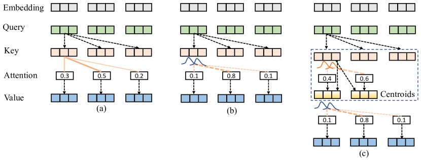
Figure 2: The illustration of multi-head self-attention in deterministic and stochastic transformers. (a) The vanilla transformer with deterministic self-attention. (b) Stochastic transformer has stochastic self-attention used to weight values $V$, the standard Softmax is replaced with the Gumbel-Softmax. (c) Hierarchical stochastic transformer learns to pay attention to values $V$ and a set of learnable centroids $C$ stochastically.

2 BACKGROUND

Predictive Uncertainty

The predictive uncertainty estimation is a challenging and unsolved problem. It has many faces, depending on different classification rules. Commonly it is classified as epistemic (model) and aleatoric (data) uncertainty (Der Kiureghian and Ditlevsen 2009; Kendall and Gal 2017). Alternatively, on the basis of input data domain, it can also be classified into in-domain (ID) (Ashukha et al. 2019) and out-of-domain (OOD) uncertainty (Hendrycks and Gimpel 2017; Wang and Van Hoof 2020). With in-domain data, i.e. the input data distribution is similar to training data distribution, a reliable model should exhibit high predictive performance (e.g., high accuracy or F1-score) and report high confidence (low uncertainty) on correct predictions. On the contrary, out-of-domain data has quite different distribution from training data, an ideal model should give high predictive performance to illustrate the generalization to unseen data distribution, but desired to be unconfident (high uncertainty). We discuss the epistemic (model) uncertainty in the context of ID and OOD scenarios in this work.

Vanilla Transformer

The vanilla transformer (Vaswani et al. 2017) is an alternative architecture to Recurrent Neural Networks recurrent neural networks (RNNs) for modelling sequential data that relaxes the model’s reliance on input sequence order. It consists of multiple components such as positional embedding, residual connection and multi-head scaled dot-product attention. The core component of the transformer is the multi-head self-attention mechanism.

Let $\mathbf{x}\in\mathbb{R}^{l\times d}$ ($l$ is sequence length, $d$ is dimension) be input data, and $\mathbf{W}_{q},\mathbf{W}_{k},\mathbf{W}_{v}\in\mathbb{R}^{d\times d}$ be the matrices for query $Q\in\mathbb{R}^{l\times h\times d_{h}}$, key $K\in\mathbb{R}^{l\times h\times d_{h}}$, and value $V\in\mathbb{R}^{l\times h\times d_{h}}$, $d_{h}=\frac{d}{h}$ and $h$ is the number of attention heads. Each $\mathbf{x}$ is associated with a query $Q$ and a key-value pair $(K,V)$. The computation of an attentive representation $A$ of $\mathbf{x}$ in the multi-head self-attention is:

$$Q =\mathbf{W}_{q}\mathbf{x};~{}~{}~{}~{}~{}~{}K=\mathbf{W}_{k}\mathbf{x};~{}~{}~{}~{}~{}~{}V=\mathbf{W}_{v}\mathbf{x};~{}~{}~{}~{}$$ (1)

$$A =\textsc{Softmax}(\alpha^{-1}QK^{\top});~{}~{}~{}~{}H=AV$$ (2)

where $H=[h_{1},...,h_{h}]$ is the multi-head output and $A=[a_{1},...,a_{h}]$ is the attention distribution that needs to attend to $V$, $\alpha$ is a scaling factor. Note that a large value of $\alpha$ pushes the Softmax function into regions where it has extremely small gradients. This attention mechanism is the key factor of a transformer for achieving high computational efficiency and excellent predictive performance. However, as we can see, all computation paths in this self-attention mechanism are deterministic, leading to a single-point output. This limits us to access and evaluate the uncertainty information beyond prediction given an input $\mathbf{x}$.

We argue that the examination of the reliability and confidence of a transformer prediction is crucial for many NLP applications, particularly when the output of a model is directly used to serve customer requests. In the following section, we introduce a simple yet efficient way to cast the deterministic attention to be stochastic for uncertainty estimation based on Gumbel-Softmax tricks (Jang, Gu, and Poole 2017; Maddison, Mnih, and Teh 2017).

3 METHODOLOGY

Bayesian Inference and Uncertainty Modeling

In this work, we focus on using transformers in classification tasks. Let $D=\{X,Y\}=\{x_{i},y_{i}\}_{i=1}^{N}$ be a training dataset, $y_{i}\in\{1,...,M\}$ is the categorical label for an input $x_{i}\in\mathbb{R}^{d}$. The goal is to learn a transformation function $f$, which is parameterized by weights $\omega$ and maps a given input $x$ to a categorical distribution $y$. The learning objective is to minimize negative log likelihood, $\mathcal{L}=-\frac{1}{N}\sum_{i}^{N}\log p(y_{i}|x_{i},\omega)$. The probability distribution is obtained by Softmax function as:

$$p(y_{i}=m|x_{i},\omega)=\frac{\exp(f_{m}(x_{i},\omega))}{\sum_{k\in M}\exp(f_{k}(x_{i},\omega)}.$$ (3)

In the inference phase, given a test sample $x^{*}$, the predictive probability $y^{*}$ is computed by:

$$p(y^{*}|x^{*},D)=\int p(y^{*}|x^{*},\omega)p(\omega|D)d\omega$$ (4)

where the posterior $p(\omega|D)$ is intractable and cannot be computed analytically. A variational posterior distribution $q_{\theta}(\omega)$, where $\theta$ are the variational parameters, is used to approximate the true posterior distribution by minimizing the Kullback-Leilber (KL) distance. This can also be treated as the maximization of evidence lower bound (ELBO):

$$\mathcal{L_{\theta}}=\int q_{\theta}(\omega)p(Y|X,\omega)d\omega-\textbf{KL}[q_{\theta}(\omega)\parallel p(\omega)]$$ (5)

With the re-parametrization trick (Kingma, Salimans, and Welling 2015), a differentiable mini-batched Monte Carlo estimator can be obtained.

The predictive (epistemic) uncertainty can be measured by performing $T$ inference runs and averaging predictions.

$$p(y*|x*)=\frac{1}{T}\sum_{t=1}^{T}p_{\omega_{t}}(y^{*}|x^{*},\omega_{t})$$ (6)

$T$ corresponds to the number of sets of mask vectors from Bernoulli distribution $\{r^{t}\}_{t=1}^{T}$ in MC-dropout, or the number of randomly trained models in Ensemble, which potentially leads to different set of learned parameters $\omega=\{\omega_{1},...,\omega_{t}\}$, or the number of sets of sampled attention distribution from Gumbel distribution $\{g^{t}\}_{t=1}^{T}$ in our proposed method.

Stochastic Self-Attention with Gumbel-Softmax

As described in section 2, the core component that makes a transformer successful is the multi-head self-attention. For each $i$-th head, let $q_{i}\in Q,k_{i}\in K,v_{i}\in V$, it is written as:

$$a_{i} =\textsc{Softmax}(\frac{q_{i}k_{i}^{\top}}{\tau});~{}~{}a_{i}\in\mathbb{R}^{l\times l}$$ (7)

$$h_{i} =a_{i}v_{i};~{}~{}~{}~{}h_{i}\in\mathbb{R}^{l\times d_{h}}$$ (8)

We here use a temperature parameter $\tau$ to replace the scaling factor $\alpha$. The $a_{i}$ is attention distribution, which learns the compatibility scores between tokens in the sequence with the $i$-th attention head. The scores are used to retrieve and form the mixture of the content of values, which is a kind of content-based addressing mechanism in neural Turing machine (Graves, Wayne, and Danihelka 2014). Note the attention is deterministic.

A straightforward way to inject stochasticity is to replace standard Softmax with Gumbel-Softmax, which helps to sample attention weights to form $\hat{a}_{i}$.

$$\hat{a_{i}} \sim\mathcal{G}(\frac{q_{i}k_{i}^{\top}}{\tau})$$ (9)

$$h_{i} =\hat{a_{i}}v_{i}$$ (10)

where $\mathcal{G}$ is Gumbel-Softmax function. The Gumbel-Softmax trick is an instance of a path-wise Monte-Carlo gradient estimator (Gumbel 1954; Maddison, Mnih, and Teh 2017; Jang, Gu, and Poole 2017). With the Gumbel trick, we can draw samples $z$ from a categorical distribution given by parameters $\bm{\theta}$, that is, $\bm{z}=\mbox{{one\_hot}}\big{(}\operatorname*{arg\,max}_{i}[g_{i}+\log\theta_{i}]\big{)},i\in[1\dots k]$, where $k$ is the number of categories and $g_{i}$ are i.i.d. samples from the Gumbel$(0,1)$, that is, $g=-\log(-\log(u)),u\sim\textsc{uniform}(0,1)$ is independent to network parameters. Because the $\operatorname*{arg\,max}$ operator breaks end-to-end differentiability, the categorical distribution $\bm{z}$ can be approximated using the differentiable Softmax function (Jang, Gu, and Poole 2017; Maddison, Mnih, and Teh 2017). Here the $\tau$ is a tunable temperature parameter equivalent to $\alpha$ in Eq. (2), Then the attention weights (scores) for values in Eq.2 can be computed as:

$$\hat{a}_{i}=\frac{\exp((\log(\theta_{i})+g_{i})/\tau)}{\sum_{j=1}^{k}\exp((\log(\theta_{t_{j}})+g_{j})/\tau)},~{}~{}i\in[1\dots k].$$ (11)

where the $\theta_{i}=q_{i}k_{i}^{\top}$. And we use the following approximation:

$$\textbf{KL}[a\parallel\hat{a}]~{}~{}~{}\text{where}~{}~{}a_{j}=\frac{a_{j}}{\sum_{k}^{i=1}a_{i}}$$ (12)

This indicates an approximation of a deterministic attention distribution $a$ with a stochastic attention distribution $\hat{a}$. With a larger $\tau$, the distribution of attention is more uniform, and with a smaller $\tau$, the attention becomes more sparse.

The trade-off between predictive performance and uncertainty estimation.

This trade-off is rooted in bias-variance trade-off. Let $\phi(x)$ be a prediction function, and $f(x)$ is the true function and $\rho$ be a constant number. The error can be computed as:

$$\xi(x)=\underbrace{(\mathbb{E}[\phi(x)-f(x)])^{2}}_{Bias^{2}}+\underbrace{(\mathbb{E}[\phi(x)-E[\phi(x)]]^{2})}_{Variance}+\underbrace{\rho}_{Const}$$ (13)

MC-dropout (Gal and Ghahramani 2016) with $T$ times Monte Carlo estimation gives a prediction $\mathbb{E}[\phi_{t}(x)],t\in T$ and predictive uncertainty, e.g., variances $Variance[\phi_{t}(x)]$ ($\rho$ is a constant number denotes irreducible error). On both in-domain and out-of-domain datasets, a good model should exhibit low bias, which ensures model generalization capability and high predictive performance. For epistemic (model) uncertainty, we expect model outputs low variance on in-domain data and high variance on out-of-domain data.

We empirically observe (from Table 1 and Table 2) that this simple modification in Eq. (9) can effectively capture the model uncertainty, but it struggles to learn a good trade-off between predictive performance and uncertainty estimation. That is, when good uncertainty estimation performance is achieved on out-of-domain data, the predictive performance on in-domain data degrades. To address this issue, we propose a hierarchical stochastic self-attention mechanism.

Hierarchical Stochastic Self-Attention

To further encourage transformer model to have stochasticity and retain predictive performance, we propose to add an additional stochastic attention before the attention that pays values. This attention forces each key head stochastically attend to a set of learnable centroids, which will be learned during back-propagation. This is equivalent to regularizing key attention heads. Similar ideas have been used to improve transformer efficiency (Vyas, Katharopoulos, and Fleuret 2020) and to improve RNN memorization (Wang and Niepert 2019).

We first define the set of $c$ centroids, $C\in\mathbb{R}^{d_{h}\times c}$ . Let each centroid $c_{i}\in\mathbb{R}^{d_{h}}$ have the same dimension with each key head $k_{j}\in\mathbb{R}^{d_{h}}$. The model will first learn to pay attention to centroids, and a new key head $\hat{k}_{j}$ is formed by weighting each centroid. Then $\hat{k}$ and a query $q$ decides the attention weights to combine values $v$. For the $i$-th head, a given query $q_{i}$, key $k_{i}$, value $v_{i}$, the stochastic self-attention can be hierarchically formulated as:

$$\hat{a}_{c} \sim\mathcal{G}(\tau_{1}^{-1}k_{i}C),~{}~{}\hat{a}_{c}\in\mathbb{R}^{l\times c}$$ (14)

$$\hat{k_{i}} =\hat{a}_{c}C^{\top},~{}~{}\hat{k_{i}}\in\mathbb{R}^{l\times d_{h}}$$ (15)

$$\hat{a}_{v} \sim\mathcal{G}(\tau_{2}^{-1}q_{i}\hat{k}_{i}^{\top}),~{}~{}\hat{a}_{v}\in\mathbb{R}^{l\times l}$$ (16)

$$h_{i} =\hat{a}_{v}v_{i}$$ (17)

$\hat{a}_{c},\hat{a}_{v}$ are the sampled categorical distributions that are used to weight centroids in $C$ and tokens in $v_{i}$. The $\tau_{1},\tau_{2}$ control the softness for each stochastic self-attention, respectively.

We summarize the main procedures of performing hierarchical stochastic attention in transformer in Algorithm 1.

Input : query $Q$, key $K$, value $V$, centroids $C$

Output : Hierarchical stochastic attentive output $H$

1 Model stochastic attention $\hat{A_{c}}$ over centroids $C$ as Eq.14;

2 Sample $\hat{A}_{c}$ from a categorical distribution $\bm{z}=\mbox{{one\_hot}}\big{(}\operatorname*{arg\,max}_{i}[g_{i}+\log\theta_{i}]\big{)},i\in[1\dots k]$, $g=-\log(-\log(u)),u\sim\textsc{uniform}(0,1)$ ;

3 Differentially approximate $\hat{A}_{c}$ as Eq. 11;

4 Compute $\hat{K}=\hat{A}_{c}C^{\top}$ as Eq. 15;

5 Model stochastic attention $\hat{A_{v}}$ over value $V$ as Eq.16;

6 Sample and approximate $\hat{A_{v}}$, similar to line 2 to 3;

7 Compute $H=\hat{A}_{v}V$ as Eq. 17;

Algorithm 1 Hierarchical stochastic transformer.

Why perform clustering on key heads?

The equation (14) performs clustering on the key attention heads and outputs an attention distribution, and equation (15) tries to form a new head based on attention distribution and learned centroids. The goal is to make the original key heads to be stochastic, allowing attention distribution to have randomness for uncertainty estimation. This goal can be also accompanied by applying equations (14) and (15) to query while keeping key unchanged. In that case, $\hat{a}_{c}$ can be still sampled stochastically based on query and centroids.

Stochastic attention approximation.

The equations (14) and (15) group the key heads into a fixed number of centroids and are reweighed by the mixture of centroids. As in (Vyas, Katharopoulos, and Fleuret 2020), we can analyze the attention approximation error, and derive that the key head attention difference is bounded.

Proposition 3.1

Given two keys $k_{i}$ and $k_{j}$ such that $\left\|k_{i}-k_{j}\right\|_{2}\leq\varepsilon$, stochastic key attention difference is bounded: $\left\|\mathcal{G}(\tau^{-1}k_{i}C))-\mathcal{G}(\tau^{-1}k_{j}C))\right\|_{2}\leq\tau^{-1}\varepsilon\left\|C\right\|_{2}$, where $\mathcal{G}$ is the Gumbel-Softmax function, and $\left\|C\right\|_{2}$ is the spectral norm of centroids. $\varepsilon$ and $\tau$ are constant numbers.

Proof 3.1

Same to the Softmax function, which has Lipschitz constant less than 1 (Gao and Pavel 2017), we have the following derivation:

$$\left\|\mathcal{G}(\tau^{-1}k_{i}C))-\mathcal{G}(\tau^{-1}k_{j}C))\right\|_{2}$$ (18)

$$~{}\leq\left\|\tau^{-1}k_{i}C-\tau^{-1}k_{j}C\right\|_{2}$$

$$~{}\leq\tau^{-1}\varepsilon\left\|C\right\|_{2}$$

Proposition 3.1 shows that the $i$-th key assigned to $j$-th centroid can be bounded by its distance from $j$-th centroid. The keys that are close in Euclidean space have similar attention distribution over centroids.

4 EXPERIMENTAL SETUPS

We design experiments to achieve the following objectives:

• To evaluate the predictive performance of models on in-domain datasets. High predictive scores and low uncertainty scores are desired.

• To compare the model generalization from in-domain to out-of-domain datasets. High scores are desired.

• To estimate the uncertainty of the models on out-of-domain datasets. High uncertainty scores are desired.

• To measure the model capability in learning the predictive performance and uncertainty estimation trade-off.

Datasets

We use IMDB dataset (Maas et al. 2011) for the sentiment analysis task. The standard IMDB has 25,000/25,000 reviews for training and test, covering 72,062 unique words. For hyperparameter selection, we take 10% of training data as validation set, leading to 22,500/2,500/25,000 data samples for training, validation, and testing. Besides, we use customer review (CR) dataset (Hendrycks and Gimpel 2017) which has 500 samples to evaluate the proposed model in OOD settings. We conduct the second experiment on linguistic acceptability task with CoLA dataset (Warstadt, Singh, and Bowman 2019). It consists of 8,551 training and 527 validation in-domain samples. As the labels of test set is not publicly available, we split randomly the 9078 in-domain samples into train/valid/test with 7:1:2. Additionally, we use the provided 516 out-of-domain samples for uncertainty estimation.

Compared Methods.

We compare the following methods in our experimental setup:

• Trans (Vaswani et al. 2017): The vanilla transformer with deterministic self-attention.

• MC-dropout (Gal and Ghahramani 2016): Using dropout (Srivastava et al. 2014) as a regularizer to measure the prediction uncertainty.

• Ensemble (Lakshminarayanan, Pritzel, and Blundell 2017): Average over multiple independently trained transformers.

• sto-trans: The proposed method that the attention distribution over values is stochastic;

• H-sto-tran: The proposed method that uses hierarchical stochastic self-attention, i.e., the stochastic attention from key heads to a learnable set of centroids and the stochastic attention to value, respectively.

Implementation details

We implement models in PyTorch (Paszke et al. 2019). The models are trained with Adam (Kingma and Ba 2014) as the optimization algorithm. For each trained model, we sample 10 predictions (run inference 10 times), the mean and variance (or standard deviation) of results are reported. The uncertainty information is quantified with variance (or standard deviation). For sentiment analysis, we use 1 layer with 8 heads, both the embedding size and the hidden dimension size are 128. We train the model with learning rate of 1e-3, batch size of 128, and dropout rate of 0.5/0.1. We evaluate models at each epoch, and the models are trained with maximum 50 epochs. We report accuracy as the evaluation metric. For linguistic acceptability, we use 8 layers and 8 heads, the embedding size is 128 and the hidden dimension is 512. We train the model with learning rate of 5e-5, batch size of 32 and dropout rate of 0.1. We train the models with maximum 2000 epochs and evaluate the models at every 50 epochs. We use Matthews correlation coefficient (MCC) (Matthews 1975) as the evaluation metric. The model selection is performed based on validation dataset according to predictive performance.

5 EXPERIMENTAL RESULTS

Results on Sentiment Analysis

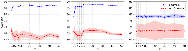
Figure 3: The experiments with hyperparameter $\tau$. Left: sto-trans with different $\tau$. The randomness is solely based on the sampling on attention distribution over values. While uncertainty information is captured, sto-trans has difficulties in learning the trade-off between in-domain and out-of-domain performance. Middle: The hyperparameter tuning of $\tau_{1}$ and $\tau_{2}$ in h-sto-trans. $\tau_{1}$ controls the concentration on centroids and $\tau_{2}$ controls the concentration on values.

	ID (%)	OOD (%)	$\bigtriangledown$ID (%)	$\bigtriangledown$OOD (%)
trans ($\eta=0.1$)	87.00	65.00	/	/
trans ($\eta=0.5$)	87.51	63.40	0.51 $\uparrow$	1.60 $\downarrow$
MC-dropout ($\eta=0.5$)	86.06 $\pm$ 0.087	63.38 $\pm$ 1.738	0.94 $\uparrow$	1.62 $\downarrow$
MC-dropout ($\eta=0.1$)	87.01 $\pm$ 0.075	63.38 $\pm$ 0.761	0.10 $\uparrow$	1.62 $\downarrow$
ensemble	86.89 $\pm$ 0.230	64.20 $\pm$ 1.585	0.11 $\downarrow$	0.80 $\downarrow$
sto-trans ($\tau=1$)	82.62 $\pm$ 0.092	67.92 $\pm$ 0.634	4.38 $\downarrow$	2.92 $\uparrow$
sto-trans ($\tau=40$)	87.42 $\pm$ 0.022	63.78 $\pm$ 0.289	0.42 $\uparrow$	1.22 $\downarrow$
h-sto-trans ($\tau_{1}=1$, $\tau_{2}=20$)	87.63 $\pm$ 0.017	67.14 $\pm$ 0.400	0.63 $\uparrow$	2.14 $\uparrow$
h-sto-trans ($\tau_{1}=1$, $\tau_{2}=30$)	87.66 $\pm$ 0.022	66.72 $\pm$ 0.271	0.66 $\uparrow$	1.72 $\uparrow$

Table 1: The predictive performance and uncertainty estimation of models on IMDB (ID) and CR (OOD) dataset. The uncertainty estimation is performed by running forward pass inference by 10 runs, then the uncertainty is quantified by standard deviation across runs. For ensemble, the results are averaged on 10 models that are independently trained with random seeds. Dropout is used in the inference of MC-dropout and $\eta$ is dropout rate. In the rest of methods, dropout is not used in inference. The $\bigtriangledown$ID (%) and $\bigtriangledown$OOD (%) present the predictive performance difference to trans ($\eta=0.1$).

Table 1 presents the predictive performance and uncertainty estimation on IMDB (in-domain, ID) and CR (out-of-domain, OOD) dataset, evaluated by accuracy.

First, sto-trans and h-sto-trans are able to provide uncertainty information, as well as maintain and even slightly outperform the predictive performance of trans. Specially, sto-trans ($\tau=40$) and h-sto-trans ($\tau_{1}=1$, $\tau_{2}=30$) outperforms trans ($\eta=0.1$) by 0.42% and 0.66% on ID dataset. In addition, they allow us to measure the uncertainty via predictive variances. It is because they inject randomness directly to self-attentions. However, trans has no access to uncertainty information due to its deterministic nature.

Second, sto-trans is struggling to learn a good trade-off between ID predictive performance and OOD uncertainty estimation performance. With small temperature $\tau=1$, sto-trans gives good uncertainty information, but we observe that the ID predictive performance drops. When $\tau$ approaches to $\sqrt{d/h}$ (the original scaling factor in the vanilla transformer), sto-trans achieves better performance on ID dataset, but lower performance on OOD dataset. We conjecture that the randomness in sto-trans is solely based on the attention distribution over values and is not enough for learning the trade-off.

Third, h-sto-trans achieves better accuracy-uncertainty trade-off compared with sto-trans. For instance, with $\tau_{1}=1,\tau_{2}=20$, h-sto-trans achieves 87.63% and 67.14%, which outperform the corresponding numbers of sto-trans for both ID and OOD datasets. It also outperforms MC-dropout and ensemble, specially, h-sto-trans outperforms 0.62%-1.6% and 2.52%-3.76% on ID and OOD datasets, respectively. On OOD dataset, while MC-dropout and ensemble exhibit higher uncertainty (measured by standard deviation) across runs, the accuracy is lower than that of trans ($\eta=0.1$), sto-trans ($\tau=1$) and h-sto-trans. It is due to a better way of learning two types of randomness: one from sampling over a set of learnable centroids and the other one from sampling attention over values.

Figure 3 reports the hyperparameter tuning of $\tau_{1}$ and $\tau_{2}$. The goal is to find a reasonable combination to achieve high predictive performance on both ID and OOD datasets. To simplify the tuning work, we fix the $\tau_{1}=1$ and then change $\tau_{2}$ with different values, and vice versa. As we can see, the combination of a small $\tau_{1}$ and a large $\tau_{2}$ performs better than the other way around. We think this is because $\tau_{2}$ is in the latter stage and has bigger effects on the predictive performance. However, removing $\tau_{1}$ goes back to Figure 3 (Left), where accuracy-uncertainty trade-off is not well learned by sto-trans.

Results on Linguistic Acceptability

Table 2 shows the performance of compared models on both in-domain (ID) and out-of-domain (OOD) sets of CoLA dataset, evaluated by MCC.

Models	ID(%)	OOD(%)	$\bigtriangledown$ID (%)	$\bigtriangledown$OOD (%)
Trans ($\eta=0.1$)	20.09	16.46	/	/
MC-dropout ($\eta=0.1$)	19.91 $\pm$ 0.40	16.70 $\pm$ 2.21	0.18 $\downarrow$	0.24 $\uparrow$
MC-dropout ($\eta=0.05$)	20.03 $\pm$ 0.30	17.11 $\pm$ 1.21	0.06 $\downarrow$	0.65 $\uparrow$
Ensemble	21.20 $\pm$ 2.59	16.73 $\pm$ 4.92	1.11 $\uparrow$	0.27 $\uparrow$
sto-trans	23.27 $\pm$ 0.75	15.25 $\pm$ 4.65	3.18 $\uparrow$	1.21 $\downarrow$
h-sto-trans	20.52 $\pm$ 0.76	16.49 $\pm$ 4.08	0.43 $\uparrow$	0.03 $\uparrow$

Table 2: The performance of compared models on CoLA dataset. We set all temperature values $\tau_{1}=1$ and $\tau_{2}=1$. The $\bigtriangledown$ID (%) and $\bigtriangledown$OOD (%) present the predictive performance and difference to trans ($\eta=0.1$), respectively.

Examples (Labels)	Prob. Corr.	Corr./Total
no man has ever beaten the centaur. (1)	0.75 $\pm$ 0.001	10/10
nora sent the book to london (1)	0.65 $\pm$ 0.007	10/10
sally suspected joe, but he did n’t holly. (1)	0.60 $\pm$ 0.008	8/10
kim is eager to recommend. (0)	0.41 $\pm$ 0.011	3/10
he analysis her was flawed (0)	0.24 $\pm$ 0.003	0/10
sandy had read how many papers ? ! (1)	0.67 $\pm$ 0.010	10/10
which book did each author recommend ? (1)	0.58 $\pm$ 0.010	7/10
she talked to harry , but i do n’t know who else .(1)	0.52 $\pm$ 0.013	4/10
john is tall on several occasions . (0)	0.42 $\pm$ 0.005	1/10
they noticed the painting , but i do n’t know for how long . (0)	0.28 $\pm$ 0.003	0/10

Table 3: Illustration of predictions with h-sto-trans. The predictions for each ID (top) and OOD (bottom) samples are measured by the probability of being correct of each prediction and the number of correct predictions.

First, sto-trans and h-sto-trans obtain comparable performance as well as provide uncertainty information, compared with trans. To be specific, sto-trans and h-sto-trans improves 3.18% and 0.43% of MCC on ID dataset compared with deterministic trans respectively.

Second, sto-trans achieves the best performance on ID dataset but the worst performance on OOD dataset. Although sto-trans outperforms trans, the best MC-dropout, ensemble by 3.18%, 3.24%, 2.07% of MCC on ID dataset, its performance drops by 1.21%, 1.86%, 1.48%, correspondingly on OOD dataset. This further verifies our conjecture that the randomness is only introduced to attention distribution over values and is insufficient for learning the trade-off of ID and OOD data.

Third, h-sto-trans enabled to learn better trade-off between prediction and uncertainty. Precisely, the performance improves 0.43% and 0.03% of MCC on ID and OOD datasets respectively. h-sto-trans is 0.49% superior to MC-dropout ($\eta=0.05$), meanwhile, 0.68% inferior to ensemble on ID dataset. Given ensemble shows high uncertainty on ID dataset and MC-dropout ($\eta=0.05$) has low uncertainty on OOD dataset, this is not desired. Therefore, h-sto-trans is the one that strikes the better balance across the objectives. In the context of this task, it means high MCC, low variance on ID dataset and high MCC, high variance on OOD dataset.

Table 3 gives some predictions of test samples with h-sto-trans. What we observed are two folds: (1) In general, ID predictions have lower variances in terms of the probability of being correct. For “10/10” (10 correct predictions out of 10 total predictions) prediction cases, the ID examples have higher probability score than the ones in OOD data. Also, we find there are much less number of “10/10” prediction cases in OOD dataset than that in ID dataset. (2) For ID dataset, either with high or low probability scores, we can see low variances, we see more “10/10” (tend to be confidently correct) or “0/10” (tend to be confidently incorrect) cases. As expected, for both cases, the variance is relatively low as compared to probability around 0.5. In deterministic models, we are not able to access this kind of information which would imply how confident are the transformer models towards predictions.

6 RELATED WORK

Bayesian neural networks (Blundell et al. 2015) inject stochasticity by sampling the network parameters from a Gaussian prior. Then the posterior distribution of target can be estimated in multiple sampling runs. However, the Bayesian approach doubles the number of network parameters, i.e., instead of learning a single-point network parameter, it learns a weight distribution which is assumed to follow a Gaussian distribution. Additionally, it often requires intensive tuning work on Gaussian mean and variance to achieve stable learning curves as well as predictive performance. MC dropout (Gal and Ghahramani 2016) approximates Bayesian approach by sampling dropout masks from a Bernoulli distribution. However, MC dropout has been demonstrated to give overconfident uncertainty estimation (Foong et al. 2019). Alternatively, the recently proposed deep ensembles (Lakshminarayanan, Pritzel, and Blundell 2017) offers possibility to estimate predictive uncertainty by combining predictions from different models which are trained with different random seeds. This, however, significantly increases the computational overhead for training and inference. There are some MC dropout based methods recently proposed. Sequential MC transformer (Martin et al. 2020), which models uncertainty by casting self-attention parameters as unobserved latent states by evolving randomly through time.  (He et al. 2020) combined mix-up, self-ensembling and dropout to achieve more accurate uncertainty score for text classification.  (Shelmanov et al. 2021) proposed to incorporate determinantal point process (DPP) to MC dropout to quantify the uncertainty of transformers. Different to the above-mentioned approaches, we inject stochasticity into the vanilla transformer with Gumbel-Softmax tricks. As it is shown in the experiment section, hierarchical stochastic self-attention component can effectively capture model uncertainty, and learn a good trade-off between in-domain predictive performance and out-of-domain uncertainty estimation.

7 DISCUSSION

While many extension of transformers have been recently proposed, the most of transformer variants are still deterministic. Our goal in this work is to equip transformers in a stochastic way to estimate uncertainty while retaining the original predictive performance. This requires special design in order to achieve the two goals without adding a major computational overhead to model training and inference like Ensembles and Bayesian Neural Network (BNN). The complexity gain of our method to its deterministic version is modest and requires an additional matrix $C\in\mathbb{R}^{d_{h}\times c}$. This is more efficient than Ensemble and BNN, which gives N ($N\geq 2$ for Ensemble and $N=2$ for BNN) times more weights.

8 CONCLUSION

This work proposes a novel, simple yet effective way to enable transformers with uncertainty estimation, as an alternative to MC dropout and ensembles. We propose variants of transformers based on two stochastic self-attention mechanisms: (1) injecting stochasticity into the stochastic attention over values; (2) forcing key heads to pay stochastic attention to a set of learnable centroids. Our experimental results show that the proposed approach learns good trade-offs between in-domain predictive performance and out-of-domain uncertainty estimation performance on two NLP benchmark tasks, and outperforms baselines.

References

- Ahmed and Torresani (2019) Ahmed, K.; and Torresani, L. 2019. Star-caps: Capsule networks with straight-through attentive routing. NeurIPS’19, 32: 9101–9110.
- Ashukha et al. (2019) Ashukha, A.; Lyzhov, A.; Molchanov, D.; and Vetrov, D. 2019. Pitfalls of in-domain uncertainty estimation and ensembling in deep learning. In ICLR’19.
- Baker et al. (2020) Baker, S. R.; Bloom, N.; Davis, S. J.; and Terry, S. J. 2020. Covid-induced economic uncertainty. Technical report, National Bureau of Economic Research.
- Blundell et al. (2015) Blundell, C.; Cornebise, J.; Kavukcuoglu, K.; and Wierstra, D. 2015. Weight uncertainty in neural network. In ICML’15, 1613–1622. PMLR.
- Der Kiureghian and Ditlevsen (2009) Der Kiureghian, A.; and Ditlevsen, O. 2009. Aleatory or epistemic? Does it matter? Structural safety, 31(2): 105–112.
- Devlin et al. (2019) Devlin, J.; Chang, M.-W.; Lee, K.; and Toutanova, K. 2019. BERT: Pre-training of deep bidirectional transformers for language understanding. In NAACL-HLT’19, 4171–4186.
- Foong et al. (2019) Foong, A. Y.; Li, Y.; Hernández-Lobato, J. M.; and Turner, R. E. 2019. ‘in-between’ uncertainty in Bayesian neural networks. In ICML’19 Workshop.
- Gal and Ghahramani (2016) Gal, Y.; and Ghahramani, Z. 2016. Dropout as a bayesian approximation: Representing model uncertainty in deep learning. In ICML’16, 1050–1059. PMLR.
- Gao and Pavel (2017) Gao, B.; and Pavel, L. 2017. On the properties of the softmax function with application in game theory and reinforcement learning. arXiv preprint arXiv:1704.00805.
- Gawlikowski et al. (2021) Gawlikowski, J.; Tassi, C. R. N.; Ali, M.; Lee, J.; Humt, M.; Feng, J.; Kruspe, A.; Triebel, R.; Jung, P.; Roscher, R.; et al. 2021. A survey of uncertainty in deep neural networks. arXiv preprint arXiv:2107.03342.
- Ghoshal and Tucker (2020) Ghoshal, B.; and Tucker, A. 2020. Estimating uncertainty and interpretability in deep learning for coronavirus (COVID-19) detection. arXiv preprint arXiv:2003.10769.
- Gillioz et al. (2020) Gillioz, A.; Casas, J.; Mugellini, E.; and Abou Khaled, O. 2020. Overview of the Transformer-based models for NLP tasks. In FedCSIS’19, 179–183. IEEE.
- Graves, Wayne, and Danihelka (2014) Graves, A.; Wayne, G.; and Danihelka, I. 2014. Neural turing machines. arXiv preprint arXiv:1410.5401.
- Gumbel (1954) Gumbel, E. J. 1954. Statistical theory of extreme values and some practical applications. A series of lectures. Number 33. US Govt. Print. Office.
- Han et al. (2021) Han, K.; Xiao, A.; Wu, E.; Guo, J.; Xu, C.; and Wang, Y. 2021. Transformer in transformer. arXiv preprint arXiv:2103.00112.
- He et al. (2020) He, J.; Zhang, X.; Lei, S.; Chen, Z.; Chen, F.; Alhamadani, A.; Xiao, B.; and Lu, C. 2020. Towards More Accurate Uncertainty Estimation In Text Classification. In EMNLP’20, 8362–8372.
- Hendrycks and Gimpel (2017) Hendrycks, D.; and Gimpel, K. 2017. A baseline for detecting misclassified and out-of-distribution examples in neural networks. In ICLR’17.
- Hoel, Wolff, and Laine (2020) Hoel, C.-J.; Wolff, K.; and Laine, L. 2020. Tactical decision-making in autonomous driving by reinforcement learning with uncertainty estimation. In 2020 IEEE Intelligent Vehicles Symposium (IV), 1563–1569. IEEE.
- Jang, Gu, and Poole (2017) Jang, E.; Gu, S.; and Poole, B. 2017. Categorical reparameterization with gumbel-softmax. In ICLR’17.
- Kabir et al. (2018) Kabir, H. D.; Khosravi, A.; Hosen, M. A.; and Nahavandi, S. 2018. Neural network-based uncertainty quantification: A survey of methodologies and applications. IEEE access, 6: 36218–36234.
- Kendall and Gal (2017) Kendall, A.; and Gal, Y. 2017. What Uncertainties Do We Need in Bayesian Deep Learning for Computer Vision? NeurIPS’17, 30: 5574–5584.
- Kingma and Ba (2014) Kingma, D. P.; and Ba, J. 2014. Adam: A method for stochastic optimization. arXiv preprint arXiv:1412.6980.
- Kingma, Salimans, and Welling (2015) Kingma, D. P.; Salimans, T.; and Welling, M. 2015. Variational dropout and the local reparameterization trick. In NeurIPS’15, volume 28, 2575–2583.
- Kingma and Welling (2014) Kingma, D. P.; and Welling, M. 2014. Auto-encoding variational bayes. In ICLR’14.
- Lakshminarayanan, Pritzel, and Blundell (2017) Lakshminarayanan, B.; Pritzel, A.; and Blundell, C. 2017. Simple and scalable predictive uncertainty estimation using deep ensembles. In NeurIPS’17.
- Lee et al. (2019) Lee, J.; Lee, Y.; Kim, J.; Kosiorek, A.; Choi, S.; and Teh, Y. W. 2019. Set transformer: A framework for attention-based permutation-invariant neural networks. In International Conference on Machine Learning, 3744–3753. PMLR.
- Lin, Engel, and Eslinger (2012) Lin, G.; Engel, D. W.; and Eslinger, P. W. 2012. Survey and evaluate uncertainty quantification methodologies. Technical report, Pacific Northwest National Lab.(PNNL), Richland, WA (United States).
- Maas et al. (2011) Maas, A. L.; Daly, R. E.; Pham, P. T.; Huang, D.; Ng, A. Y.; and Potts, C. 2011. Learning word vectors for sentiment analysis. In NAACL-HLT’11, 142–150. Portland, Oregon, USA: Association for Computational Linguistics.
- Maddison, Mnih, and Teh (2017) Maddison, C. J.; Mnih, A.; and Teh, Y. W. 2017. The concrete distribution: A continuous relaxation of discrete random variables. In ICLR’17.
- Martin et al. (2020) Martin, A.; Ollion, C.; Strub, F.; Corff, S. L.; and Pietquin, O. 2020. The Monte Carlo Transformer: a stochastic self-attention model for sequence prediction. arXiv preprint arXiv:2007.08620.
- Matthews (1975) Matthews, B. W. 1975. Comparison of the predicted and observed secondary structure of T4 phage lysozyme. Biochimica et Biophysica Acta (BBA)-Protein Structure, 405(2): 442–451.
- Oh and Hong (2021) Oh, G.; and Hong, Y. S. 2021. Managing market risk caused by customer preference uncertainty in product family design with launch flexibility: Product option strategy. Computers & industrial engineering, 151: 106975.
- Paszke et al. (2019) Paszke, A.; Gross, S.; Massa, F.; Lerer, A.; Bradbury, J.; Chanan, G.; Killeen, T.; Lin, Z.; Gimelshein, N.; Antiga, L.; Desmaison, A.; Kopf, A.; Yang, E.; DeVito, Z.; Raison, M.; Tejani, A.; Chilamkurthy, S.; Steiner, B.; Fang, L.; Bai, J.; and Chintala, S. 2019. PyTorch: An imperative style, high-performance deep learning library. In Wallach, H.; Larochelle, H.; Beygelzimer, A.; d'Alché-Buc, F.; Fox, E.; and Garnett, R., eds., NeuIPS’19, 8024–8035.
- Ren et al. (2021) Ren, P.; Chen, Z.; Ren, Z.; Kanoulas, E.; Monz, C.; and De Rijke, M. 2021. Conversations with search engines: SERP-based conversational response generation. TOIS’20, 39(4): 1–29.
- Riedmaier et al. (2021) Riedmaier, S.; Danquah, B.; Schick, B.; and Diermeyer, F. 2021. Unified framework and survey for model verification, validation and uncertainty quantification. Archives of Computational Methods in Engineering, 28(4): 2655–2688.
- Shelmanov et al. (2021) Shelmanov, A.; Tsymbalov, E.; Puzyrev, D.; Fedyanin, K.; Panchenko, A.; and Panov, M. 2021. How certain is your transformer? In EACL’21, 1833–1840.
- Srivastava et al. (2014) Srivastava, N.; Hinton, G.; Krizhevsky, A.; Sutskever, I.; and Salakhutdinov, R. 2014. Dropout: A simple way to prevent neural networks from overfitting. Journal of Machine Learning Research, 15(56): 1929–1958.
- Tetko et al. (2020) Tetko, I. V.; Karpov, P.; Van Deursen, R.; and Godin, G. 2020. State-of-the-art augmented NLP transformer models for direct and single-step retrosynthesis. Nature communications, 11(1): 1–11.
- Vaswani et al. (2017) Vaswani, A.; Shazeer, N.; Parmar, N.; Uszkoreit, J.; Jones, L.; Gomez, A. N.; Kaiser, Ł.; and Polosukhin, I. 2017. Attention is all you need. In NeurIPS’17, 5998–6008.
- Vyas, Katharopoulos, and Fleuret (2020) Vyas, A.; Katharopoulos, A.; and Fleuret, F. 2020. Fast transformers with clustered attention. NeuIPS’20.
- Wang et al. (2020) Wang, B.; Shang, L.; Lioma, C.; Jiang, X.; Yang, H.; Liu, Q.; and Simonsen, J. G. 2020. On position embeddings in bert. In ICLR’20.
- Wang, Lawrence, and Niepert (2021) Wang, C.; Lawrence, C.; and Niepert, M. 2021. Uncertainty Estimation and Calibration with Finite-State Probabilistic RNNs. In ICLR’21.
- Wang and Niepert (2019) Wang, C.; and Niepert, M. 2019. State-regularized recurrent neural networks. In ICML’19, 6596–6606. PMLR.
- Wang and Van Hoof (2020) Wang, Q.; and Van Hoof, H. 2020. Doubly Stochastic Variational Inference for Neural Processes with Hierarchical Latent Variables. In ICML’20, 10018–10028. PMLR.
- Warstadt, Singh, and Bowman (2019) Warstadt, A.; Singh, A.; and Bowman, S. R. 2019. Neural network acceptability judgments. Transactions of the Association for Computational Linguistics, 7: 625–641.