$B\!\to\!D^{(*)}\ell\nu$ semileptonic decays in lattice QCD with domain-wall heavy quarks

Abstract

We calculate the $B\!\to\!D^{(*)}\ell\nu$ form factors in 2+1 flavor relativistic lattice QCD by employing the Möbius domain-wall action for all quark flavors. Our simulations are carried out at lattice cut-offs $a^{-1}\sim 2.5$, 3.6 and 4.5 GeV with the bottom quark masses up to 0.7 $a^{-1}$ to control discretization effects. We extrapolate the form factors to the continuum limit and physical quark masses, and discuss systematic uncertainties of the form factors.

1 Introduction

The $B\to D^{(*)}\ell\nu$ semileptonic decays provide a determination of the Cabibbo-Kobayashi-Maskawa (CKM) matrix element $|V_{cb}|$, and are promising probes of new physics, such as the charged Higgs bosons predicted by supersymmetry. However, the current estimate of $|V_{cb}|$ shows a tension with its alternative determination from the inclusive decay [1]. It is unlikely that the tension is a sign of new physics [2] and, hence, we need deeper understanding and better control of theoretical and experimental uncertainties. In this article, we report on our calculation of the $B\!\to\!D^{(*)}\ell\nu$ form factors, which are the source of the largest theoretical uncertainty of $|V_{cb}|$.

2 Simulation method

Table 1: Simulation parameters. Light and strange quark masses, $m_{ud}$ and $m_{s}$, represent their bare values in lattice units.

lattice parameters	$m_{ud}$	$m_{s}$	$M_{\pi}$[MeV]	$M_{K}$[MeV]
$\beta\!=\!4.17$,  $a^{-1}\!=\!2.453(4)$,  $32^{3}\!\times\!64\!\times\!12$	0.0190	0.0400	499(1)	618(1)
	0.0120	0.0400	399(1)	577(1)
	0.0070	0.0400	309(1)	547(1)
	0.0035	0.0400	230(1)	527(1)
$\beta\!=\!4.17$,  $48^{3}\!\times\!96\!\times\!12$	0.0035	0.0400	226(1)	525(1)
$\beta\!=\!4.35$,  $a^{-1}\!=\!3.610(9)$,  $48^{3}\!\times\!96\!\times\!8$	0.0120	0.0250	501(2)	620(2)
	0.0080	0.0250	408(2)	582(2)
	0.0042	0.0250	300(1)	547(2)
$\beta\!=\!4.47$,  $a^{-1}\!=\!4.496(9)$,  $64^{3}\!\times\!128\!\times\!8$	0.0030	0.0150	284(1)	486(1)

We simulate $N_{f}\!=\!2+1$ lattice QCD at cutoffs of $a^{-1}\!\simeq\!2.5$ – 4.5 GeV. The pion mass is as low as $M_{\pi}\!\sim\!230$ MeV, and the strange quark mass is close to its physical value. The Möbius domain-wall action [3, 4] is employed for all relevant quark flavors to preserve chiral symmetry to good accuracy, which simplifies the renormalization of the relevant matrix elements. The charm quark mass $m_{c}$ is set to its physical value fixed from the spin averaged mass $(M_{\eta_{c}}+3M_{J/\Psi})/4$. Depending on the lattice spacing $a$, we take three to six values of the bottom quark mass $m_{b}\!=\!1.25^{n}m_{c}(n=0,1,...)$ below $0.7\,a^{-1}$ in order to control $O((am_{b})^{2})$ discretization effects. The spatial lattice size $L$ is chosen to satisfy the condition $M_{\pi}L\!\gtrsim\!4$ to suppress finite volume effects (FVEs). At our smallest $M_{\pi}\!\simeq\!230$ MeV, we simulate a smaller lattice size $M_{\pi}L\!\sim\!3$ to directly study the FVEs. The statistics are 5,000 Molecular Dynamics time at each simulation point. These simulation parameters are listed in Table 1. The same gauge ensembles are used in our study of the $B\!\to\!\pi\ell\nu$ [5] and inclusive decays [6] and in a joint project with the RBC/UKQCD Collaboration on the $B$ meson mixing [7].

The $B\!\to\!D^{(*)}$ matrix elements are parametrized by six form factors in total,

$$\sqrt{M_{B}M_{D}}^{-1}\langle D({p^{\prime}})|V_{\mu}|B(p)\rangle = (v+v^{\prime})_{\mu}h_{+}(w)+(v-v^{\prime})_{\mu}h_{-}(w),$$ (1)

$$\sqrt{M_{B}M_{D^{*}}}^{-1}\langle D^{*}(\epsilon,{p^{\prime}})|V_{\mu}|B(p)\rangle = i\varepsilon_{\mu\nu\rho\sigma}\,\epsilon^{*\nu}v^{\prime\rho}v^{\sigma}\,h_{V}(w),$$ (2)

$$\sqrt{M_{B}M_{D^{*}}}^{-1}\langle D^{*}(\epsilon,{p^{\prime}})|A_{\mu}|B(p)\rangle = (w+1)\,\epsilon_{\mu}^{*}\,h_{A_{1}}(w)-(\epsilon^{*}v)\,v_{\mu}\,h_{A_{2}}(w)-(\epsilon^{*}v)\,v^{\prime}_{\mu}\,h_{A_{3}}(w),\hskip 28.45274pt$$ (3)

where $w=vv^{\prime}$ is the recoil parameter defined by four velocities $v\!=\!p/M_{B}$ and $v^{\prime}\!=\!{p^{\prime}}/M_{D^{(*)}}$, and $\epsilon$ is the polarization vector of $D^{*}$, which satisfies ${p^{\prime}}\epsilon\!=\!0$.

The $B\!\to\!D^{(*)}$ matrix elements can be extracted from three- and two-point functions, provided that they are dominated by their ground state contribution as

$$C_{\mathcal{O}_{\Gamma}}^{BD^{(*)}}({\Delta t},{\Delta t^{\prime}};{\bf p},{{\bf p}^{\prime}})$$ (4)

$$= \sum_{{{\bf x}_{\rm src}},{\bf x},{{\bf x}^{\prime}}}\langle{\mathcal{O}}_{D^{(*)}}({{\bf x}^{\prime}},{\Delta t}+{\Delta t^{\prime}}){\mathcal{O}}_{\Gamma}({\bf x},{\Delta t}){\mathcal{O}}_{B}({{\bf x}_{\rm src}},0)^{\dagger}\rangle e^{-i{\bf p}({\bf x}-{{\bf x}_{\rm src}})-i{{\bf p}^{\prime}}({{\bf x}^{\prime}}-{\bf x})}$$

$$\xrightarrow[{\Delta t},{\Delta t^{\prime}}\to\infty]{} \frac{Z_{D^{(*)}}^{*}({{\bf p}^{\prime}})\,Z_{B}({\bf p})}{4E_{D^{(*)}}({{\bf p}^{\prime}})E_{B}({\bf p})}\langle D^{(*)}({p^{\prime}})|{\mathcal{O}}_{\Gamma}|B(p)\rangle e^{-E_{D^{(*)}}({{\bf p}^{\prime}}){\Delta t^{\prime}}-E_{B}({\bf p}){\Delta t}}.$$

Here ${\mathcal{O}}_{\Gamma}\!=\!V_{\mu}$ or $A_{\mu}$, and the argument $\epsilon$ is suppressed for $Z_{D^{*}}$ and $|D^{*}({p^{\prime}})\rangle$ for simplicity. We apply Gaussian smearing to the interpolating fields ${\mathcal{O}}_{P}$ of the mesons $P\!=\!B,D,D^{*}$ to enhance their overlap with the ground state $Z_{P}({\bf p})\!=\!\langle P(p)|{\mathcal{O}}_{P}^{\dagger}\rangle$. The $B$ meson is at rest (${\bf p}\!=\!{\bf 0}$) throughout our measurements, whereas we vary the three momentum of $D^{(*)}$ as $|{{\bf p}^{\prime}}|^{2}\!=\!0,1,2,3,4$ in units of $(2\pi/L)^{2}$ in order to study the $w$ dependence of the form factors.

We construct ratios of the correlation functions as

$$R_{(k)}^{BD^{(*)}}({\Delta t},{\Delta t^{\prime}}) = \frac{C_{V_{4}(A_{k})}^{BD^{(*)}}({\Delta t},{\Delta t^{\prime}};{\bf 0},{\bf 0})\,C_{V_{4}(A_{k})}^{D^{(*)}B}({\Delta t},{\Delta t^{\prime}};{\bf 0},{\bf 0})}{C_{V_{4}}^{BB}({\Delta t},{\Delta t^{\prime}};{\bf 0},{\bf 0})\,C_{V_{4}}^{D^{(*)}D^{(*)}}({\Delta t},{\Delta t^{\prime}};{\bf 0},{\bf 0})}\xrightarrow[{\Delta t},{\Delta t^{\prime}}\to\infty]{}|h_{+(A_{1})}(1)|^{2},$$ (5)

$$R_{V,k}^{BD^{*}}({\Delta t},{\Delta t^{\prime}};{\bf 0},{\bf p}_{\perp}^{\prime}) = \frac{C_{V_{k}}^{BD^{*}}({\Delta t},{\Delta t^{\prime}};{\bf 0},{\bf p}_{\perp}^{\prime})}{C_{A_{k}}^{BD^{*}}({\Delta t},{\Delta t^{\prime}};{\bf 0},{\bf p}_{\perp}^{\prime})}\xrightarrow[{\Delta t},{\Delta t^{\prime}}\to\infty]{}\frac{\epsilon_{kij}\epsilon^{*}_{i}v_{\perp j}^{\prime}}{1+w}\frac{h_{V}(w)}{h_{A}(w)}$$ (6)

where ${\bf p}_{\perp}^{\prime}$ denotes the $D^{*}$ momentum satisfying $v\epsilon\!=\!0$. Unnecessary factors, such as the overlap $Z_{P}({\bf p})$ and exponential damping factors in Eq. (4), cancel in the ratios [8]. We also expect a partial cancellation of statistical fluctuations. These ratios are used to precisely extract the form factors at zero recoil, $h_{+}(1)$ and $h_{A_{1}}(1)$ and a ratio $R_{1}(w)\!=\!h_{V}(w)/h_{A_{1}}(w)$, which are key hadronic inputs in the conventional determination of $|V_{cb}|$. We refer the reader to Refs. [9, 10] for ratios to extract other form factors.

In order to control the excited state contamination, we calculate the correlator ratios with four different values of the source-sink separation ${\Delta t}+{\Delta t^{\prime}}$, and then extract form factors by using multi-exponential fits. The fitting form, for instance, to determine $h_{A_{1}}(1)$ is

$$R_{1}^{BD^{*}}({\Delta t},{\Delta t^{\prime}}) = |h_{A_{1}}(1)|^{2}\left(1+ae^{-\Delta M_{B}{\Delta t}}+be^{-\Delta M_{D^{*}}{\Delta t}}+ce^{-\Delta M_{B}{\Delta t^{\prime}}}+de^{-\Delta M_{D^{*}}{\Delta t^{\prime}}}\right),$$ (7)

where $\Delta M_{B(D^{*})}$ represents the energy difference between the $B(D^{*})$ meson ground state and the first excited state with the same quantum numbers, and is estimated from two-point functions of $B$ ($D^{*}$). As plotted in Fig. 1, the multiple values of ${\Delta t}+{\Delta t^{\prime}}$ enable us to safely identify the ground state contribution, whereas data at small ${\Delta t}+{\Delta t^{\prime}}$ are helpful in achieving good statistical accuracy.

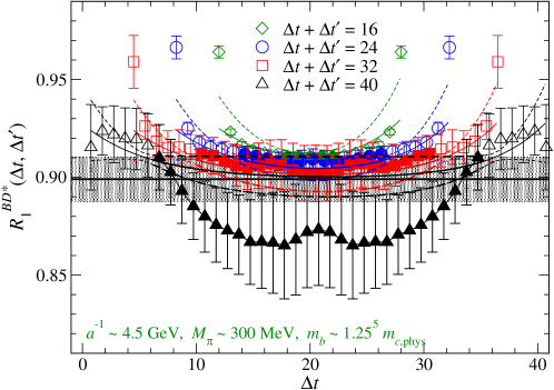
Figure 1: Double ratio $R_{1}^{BD^{*}}({\Delta t},{\Delta t^{\prime}})$ as a function of the temporal location $\Delta t$ of $A_{1}$. We plot data at $\beta\!=\!4.35$, $m_{ud}\!=\!0.0042$ and $m_{b}\!=\!1.25^{5}\,m_{c}$. Diamonds, circles, squares and triangles show data with the source – sink separation ${\Delta t}+{\Delta t^{\prime}}\!=\!16$, 24, 32 and 40, respectively. We also plot the multi-exponential fit (7) by the dashed lines, and the ground state contribution $|h_{A_{1}}(1)|^{2}$ by the black shaded band.

A salient feature of our simulations with relativistic heavy quarks and chiral symmetry is that the form factors in the Standard Model, namely those in Eqs. (1) – (3), can be calculated without finite renormalization of the lattice operators $V_{\mu}$ and $A_{\mu}$. Our correlator ratios are constructed so that renormalization factors cancel as seen in Eqs. (5) and (6). This is an important advantage, because it is not straightforward to reliably estimate and reduce higher order corrections in the perturbative renormalization and matching.

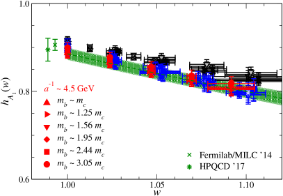
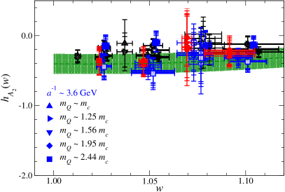
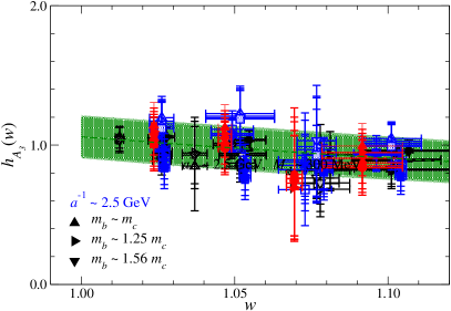
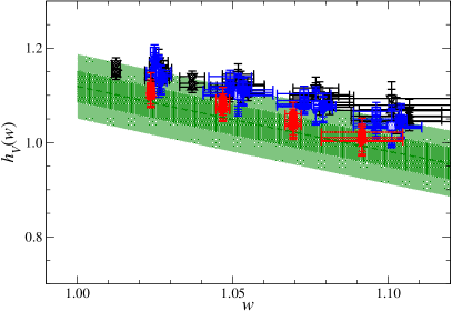
Figure 2: $B\!\to\!D^{*}\ell\nu$ form factors, $h_{A_{1}}$ (top-left), $h_{A_{2}}$ (top-right), $h_{A_{3}}$ (bottom-left) and $h_{V}$ (bottom-right) as a function of $w$. In all panels, we plot data at $a^{-1}\!=\!2.5$, 3.6 and 4.5 GeV by the black, blue and red symbols, respectively. The open, pale shaded, filled, dark shaded symbols show data at $M_{\pi}\!\sim\!500$, 400, 300 and 230 MeV, whereas symbols with different shapes are data with different values of $m_{b}$. We plot the form factors extrapolated to the continuum limit and physical quark masses by the green bands, and their statistical (total) uncertainty is shown by the dark (pale) bands. We also plot the previous estimates of $h_{A_{1}}(1)$ [16, 17], which is shifted in the horizontal direction for clarity.

3 Continuum and chiral extrapolation

We extrapolate the form factors to the continuum limit and physical quark masses by employing a fitting form with a chiral logarithm predicted by next-to-leading order heavy meson chiral perturbation theory [11, 12] and polynomial corrections. The fitting form for $h_{A_{1}}$, for instance, is

$$\frac{h_{A_{1}}}{\eta_{A}} = c+c_{w}(w-1)+d_{w}(w-1)^{2}+c_{b}(w-1){\epsilon_{b}}+d_{b}{\epsilon_{b}}^{2}$$ (8)

$$+\frac{{g_{D^{*}D\pi}}^{2}}{32\pi^{2}f_{\pi}^{2}}\bar{F}\!\left({\xi_{\pi}},\Delta_{c}\right)+c_{\pi}{\xi_{\pi}}+c_{\eta_{s}}{\xi_{\eta_{s}}}+c_{a}{\xi_{a}}+c_{am_{b}}{\xi_{am_{b}}},$$

where $\eta_{A}$ represents the one-loop radiative correction evaluated by using our estimate of the strong coupling from charmonium correlators [13]. The polynomial corrections are written in terms of small expansion parameters

$$w-1,\hskip 5.69054pt{\epsilon_{b}}=\frac{\bar{\Lambda}}{2m_{b}},\hskip 5.69054pt{\xi_{\pi}}=\frac{M_{\pi}^{2}}{(4\pi f_{\pi})^{2}},\hskip 5.69054pt{\xi_{\eta_{s}}}=\frac{M_{\eta_{s}}^{2}}{(4\pi f_{\pi})^{2}},\hskip 5.69054pt{\xi_{a}}=(\Lambda a)^{2},\hskip 5.69054pt{\xi_{am_{b}}}=(am_{b})^{2},$$ (9)

where we set $\bar{\Lambda},\Lambda\!=\!0.5$ GeV. For $h_{A_{1}}$ and $h_{+}$, the $O({\epsilon_{b}})$ term has an additional factor of $w-1$ to be consistent with Luke’s theorem [14], and we include an $O({\epsilon_{b}}^{2})$ correction as in Eq. (8).

For the chiral expansion, we employ the so-called $\xi$-expansion in ${\xi_{\pi}}$ and ${\xi_{\eta_{s}}}$, with which we observe better convergence for the light meson observables than the $x$-expansion in $M_{\pi}^{2}/(4\pi F)^{2}$ and $M_{\eta_{s}}^{2}/(4\pi F)^{2}$, where $F$ is the decay constant in the chiral limit [15].

The explicit form of the loop integral function for the chiral logarithm is given in Refs. [11, 12], and can be approximated as $\bar{F}\!=\!\Delta_{c}^{2}\ln[{\xi_{\pi}}]+O(\Delta_{c}^{3})$, where $\Delta_{c}$ represents the $D^{*}$ – $D$ mass splitting. The $D^{*}D\pi$ coupling is set to ${g_{D^{*}D\pi}}\!=\!0.53(8)$, which is quoted in Ref. [16] and the error covers previous estimates. This choice, however, has small impact on the continuum and chiral extrapolation, since the chiral logarithm is suppressed by the small mass splitting $\Delta_{c}$.

In Fig. 2, we plot the $B\!\to\!D^{*}\ell\nu$ form factors at simulation points and those extrapolated to the continuum limit and physical quark masses. With our choice of the expansion parameters (9), all coefficients $c_{\{w,b,\pi,\eta_{s},a,am_{b}\}}$ and $d_{\{w,b\}}$ turn out to be $O(1)$ or smaller. The figure suggests that the form factors mildly depend on $a$ and quark masses. Consequently, the fitting form (8) describes our data well with $\chi^{2}/{\rm d.o.f}\!\sim\!0.2$, and many coefficients are consistent with zero. We also note that our result for $h_{A_{1}}(1)$ is in reasonable agreement with the previous estimates by Fermilab/MILC [16] and HPQCD [17].

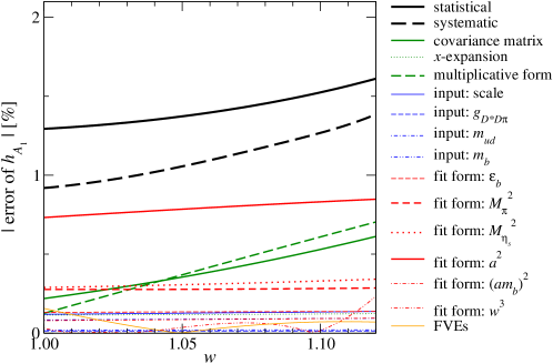
Figure 3: Uncertainties of $h_{A_{1}}(w)$ in the continuum limit and at physical quark masses. We plot the statistical (black thick solid line) and total systematic (black thick dashed line) errors, and the breakdown of the latter (other thin lines) as a function of $w$.

We estimate the following systematic errors, and plot them in Fig. 3.

• Covariance matrix : With our statistics, the covariance matrix has exceptionally small eigenvalues. We test the singular value decomposition cut as well as the shrinkage method [18], and the change of the form factors is taken as a systematic uncertainty.

• Chiral expansion : We test the $x$-expansion instead of the $\xi$-expansion.

• Multiplicative form : We test the following multiplicative fitting form in order to take account of possible cross terms,

  $$\frac{h_{A_{1}}}{\eta_{A}} = c-1+\left(1+c_{w}(w-1)+d_{w}(w-1)^{2}\right)\left(1+c_{b}(w-1){\epsilon_{b}}+d_{b}{\epsilon_{b}}^{2}\right)$$ (10)

  $$\times\left(1+\frac{{g_{D^{*}D\pi}}^{2}}{32\pi^{2}f_{\pi}^{2}}\bar{F}+c_{\pi}{\xi_{\pi}}\right)\left(1+c_{\eta_{s}}{\xi_{\eta_{s}}}\right)\left(1+c_{a}{\xi_{a}}\right)\left(1+c_{am_{b}}{\xi_{am_{b}}}\right).$$

• Inputs : We repeat the fit with $a$ and ${g_{D^{*}D\pi}}$ shifted by their uncertainty.

• Strong isospin breaking : We shift the input $M_{\pi}$ to fix $m_{ud}$ by a relative difference $2|(M_{\pi^{0}}-M_{\pi^{\pm}})|/(M_{\pi^{0}}+M_{\pi^{\pm}})$ to take account of the uncertainty due to strong isospin breaking. We carry out a similar analysis for $M_{\eta_{b}}$ to fix $m_{b}$.

• Polynomial correction : In order to estimate the systematic uncertainty due to the choice of the polynomial correction in Eq. (8), we repeat the fit by adding a higher order term or removing a poorly-determined term.

• FVEs : The form factor data at $a^{-1}\!=2.453$ GeV, $M_{\pi}\!=\!226$ MeV is replaced by those calculated on a smaller lattice $32^{3}\times 64$ to estimate FVEs.

As seen in Fig. 3, each systematic error of $h_{A_{1}}$ is suppressed well below the statistical error of 1 – 2 %. Other form factors have larger and more dominant statistical errors. With the exception of $h_{V}$, where the discretization error is 5 % and the statistical error is 3 %, all other systematic errors for each of the form factors are suppressed such that they are similar or smaller than their corresponding statistical uncertainties.

Based on the continuum and chiral extrapolation, we can generate synthetic data of the form factors. A model independent parametrization of them and comparison with the previous study [10] are in progress [19].

4 Form factor beyond the SM

One of the the so-called B physics anomalies has been reported for the decay rate ratio to measure the lepton flavor universality violation $R(D^{(*)})\!=\!\Gamma(B\!\to\!D^{(*)}\tau\nu)/\Gamma(B\!\to\!D^{(*)}\ell\nu)$ ($\ell=e,\mu$), which currently poses a 3 $\sigma$ tension between the SM and experiment. In order to interpret such a hint based on new physics models, lattice QCD is expected to provide form factors beyond the SM, namely those for the (pseudo-)scalar and tensor interactions.

Figure 4 shows our preliminary results for the $B\!\to\!D\ell\nu$ tensor form factor $h_{T}$ defined by

$$\sqrt{M_{B}M_{D}}^{-1}\langle D({p^{\prime}})\left|\bar{c}\sigma_{\mu\nu}b\right|B(p)\rangle = ih_{T}(w)(v^{\prime}_{\mu}v_{\nu}-v^{\prime}_{\nu}v_{\mu}).$$ (11)

We use a correlator ratio

$$R_{T}^{BD}({\Delta t},{\Delta t^{\prime}};{\bf 0},{\bf p}) = \frac{C_{T_{k4}}^{BD}({\Delta t},{\Delta t^{\prime}};{\bf 0},{\bf p})\,C^{D}({\Delta t^{\prime}};{\bf 0})}{C_{V_{4}}^{BD}({\Delta t},{\Delta t^{\prime}};{\bf 0},{\bf 0})\,C^{D}({\Delta t^{\prime}};{\bf p})}\xrightarrow[{\Delta t},{\Delta t^{\prime}}\to\infty]{}\frac{v_{k}}{2}\frac{h_{T}(w)}{h_{+}(1)},$$ (12)

where $C^{D}$ represents the $D$ meson two-point function, and $h_{+}(1)$ is calculated from Eq. (5). In contrast to the calculation of the SM form factors, renormalization factors do not cancel in the ratio $R_{T}^{BD}$. A non-perturbative renormalization based on the Borel transformation of the hadronic vacuum polarization function is in progress [20]. In the following, we consider $h_{T}(w)$ normalized at $w\!=\!1$ so that renormalization factor cancels.

We observe that the tensor form factor mildly depends on the lattice spacing and quark masses, and carry out the continuum and chiral extrapolation by using a fitting form similar to Eq. (8). Figure 4 shows $h_{T}(w)/h_{T}(1)$ in the continuum limit and at physical quark masses. The preliminary result has 10 % statistical and 10 % systematic errors, and is consistent with previous phenomenological estimates [21, 22].

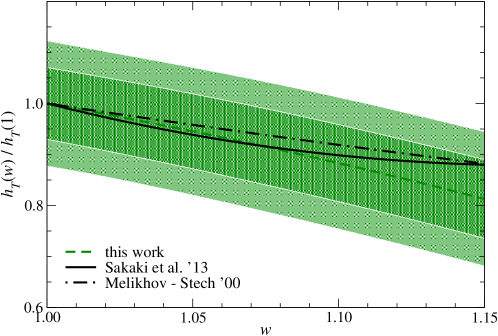
Figure 4: Tensor form factor for $B\!\to\!D\ell\nu$ decay normalized at $w\!=\!1$. Our result extrapolated to the continuum limit and physics quark masses is plotted by the green dashed line with the dark and pale green bands representing the statistical and total uncertainties, respectively. We also plot phenomenological estimates in Refs. [21, 22].

5 Summary

In this article, we report on our study of the $B\!\to\!D^{(*)}\ell\nu$ form factors at non-zero recoil in lattice QCD with domain-wall heavy quarks. The SM form factors do not need explicit renormalization thanks to chiral symmetry. The mild dependence of the form factors on simulation parameters brings the continuum and chiral extrapolation under reasonable control. As a result, the axial form factor $h_{A_{1}}$ is determined with an accuracy of $\lesssim 2$ % in the simulation region of $w$. Our study is being extended to form factors beyond the SM, and we are calculating the $B\!\to\!D\ell\nu$ tensor form factor. Implications of our results on the determination of $|V_{cb}|$ and new physics searches are under investigation.

This work used computational resources of supercomputer Fugaku provided by the RIKEN Center for Computational Science and Oakforest-PACS provided by JCAHPC through the HPCI System Research Projects (Project ID: hp180132, hp190118 and hp210146) and Multidisciplinary Cooperative Research Program in Center for Computational Sciences, University of Tsukuba (Project ID: xg18i016). This work is supported in part by JSPS KAKENHI Grant Numbers 18H03710 and 21H01085 and by the Toshiko Yuasa France Japan Particle Physics Laboratory (TYL-FJPPL project FLAV_03).

References

- [1] Y. Amhis et al. (Heavy Flavor Averaging Group), Eur. Phys. J. C 81 (2021) 226.
- [2] A. Crivellin and S. Pokorski, Phys. Rev. Lett. 114 (2015) 011802.
- [3] R.C. Brower, H. Neff and K. Orginos, Nucl. Phys. (Proc.Suppl.) 140 (2005) 686.
- [4] T. Kaneko et al. (JLQCD Collaboration), PoS (LATTICE 2013) 125.
- [5] B. Colquhoun et al. (JLQCD Collaboration), PoS (LATTICE2019) 143.
- [6] S. Mächler et al., PoS (LATTICE2021) 512 in these proceedings; S. Hashimoto et al., PoS (LATTICE2021) 534 in these proceedings.
- [7] P. Boyle et al. (RBC/UKQCD and JLQCD Collaborations), PoS (LATTICE2021) 224 in these proceedings.
- [8] S. Hashimoto et al., Phys. Rev. D61 (1999) 014502.
- [9] T. Kaneko et al. (JLQCD Collaboration), PoS (LATTICE2018) 311.
- [10] A. Bazavov et al. (Fermilab and MILC Collaboration), arXiv:2105.14019 [hep-lat].
- [11] L. Randall and M.B. Wise, Phys. Lett. B303 (1993) 135.
- [12] M.J. Savage, Phys. Rev. D65 (2002) 034014.
- [13] K. Nakayama, B. Fahy and S. Hashimoto, Phys. Rev. D94 (2016) 054507
- [14] M.E. Luke, Phys. Lett. B252 (1990) 447.
- [15] J. Noaki et al. (JLQCD and TWQCD Collaborations), Phys. Rev. Lett. 101 (2008) 202004.
- [16] J.A. Bailey et al. (Fermilab and MILC Collaboration), Phys. Rev. D 89 (2014) 114504.
- [17] J. Harrison et al. (HPQCD Collaboration), Phys. Rev. D 97 (2018) 054502.
- [18] C. Stein, in Proceedings of the Third Berkeley Symposium on Mathematical Statistics and Probability, Vol. 1, pp. 197-206; O. Ledoit and M. Wolf, J. Multivariate Anal. 88 (2004) 365.
- [19] T. Kaneko, PoS (CKM2021) 048.
- [20] T. Ishikawa, S. Hashimoto and T. Kaneko, PoS (LATTICE2021) 581 in these proceedings.
- [21] Y. Sakaki, M. Tanaka, A. Tayduganov and R. Watanabe, Phys. Rev. D 88 (2013) 094012.
- [22] D. Melikhov and B. Stech, Phys. Rev. D 62 (2000) 014006.