Relativistic entropy production for quantum field in cavity

Abstract

A nonuniformly accelerated quantum field in a cavity undergoes the coordinate transformation of annihilation and creation operators, known as the Bogoliubov transformation. This study considers the entropy production of a quantum field in a cavity induced by the Bogoliubov transformation. By classifying the modes in the cavity into the system and environment, we obtain the lower bound of the entropy production, defined as the sum of the von Neumann entropy in the system and the heat dissipated to the environment. This lower bound represents the refined second law of thermodynamics for a quantum field in a cavity and can be interpreted as the Landauer principle, which yields the thermodynamic cost of changing information contained within the system. Moreover, it provides an upper bound for the quantum mutual information to quantify the extent of the information scrambling in the cavity due to acceleration.

I Introduction

The validity of classical mechanics is challenged in processes involving massive spatial scale as relativistic effects become nonnegligible at this scale. For instance, clocks in satellites of the global positioning system (GPS) tick faster than those on the ground owing to speed and gravity, and thus, the accuracy of GPS deteriorates without considering the relativistic effects. About half a century ago, the discoveries of Hawking radiation [1] and Unruh effect [2] revealed that incorporating relativistic effects in quantum mechanics can yield surprising phenomena that cannot be realized through conventional quantum mechanics. However, more recently, certain concepts in quantum information, such as entanglement, have been recognized as crucial in relativistic settings [3, 4]. Currently, an entanglement distribution was performed between a satellite and receivers on the ground located 1200 km apart [5]. Against this background, relativistic quantum information has garnered considerable research attention, focusing on the relativistic effects of quantum information, e.g., Unruh [2] and dynamical Casimir effects [6], using the quantum field theory [7, 8, 9, 10, 11, 12].

Quantum thermodynamics is an extension of the stochastic thermodynamics operating at the mesoscopic scale to quantum microscopic scale. It generalizes the concept of stochastic work, heat, and entropy to the quantum domain, and accordingly, several thermodynamic relations, e.g., Jarzynski equality [13], fluctuation theorem [14, 15, 16], and thermodynamic uncertainty relation [17, 18], have been demonstrated to hold in the quantum domain as well [19, 20, 21]. Recently, the thermodynamic quantities and relations have been further generalized to quantum field theory. References [22] and [23] derived the Jarzynski equality for quantum field theory in a flat spacetime using two-point and indirect measurements, respectively. Regarding the quantum thermodynamics for quantum field theory in a curved spacetime, Ref. [24] investigated the work exerted by the expanding universe. Moreover, Ref. [25] considered several quantities to formulate the quantum thermodynamics of a quantum field in an accelerating cavity.

Herein, we study the entropy production [26] in a quantum field confined in a cavity that undergoes acceleration. In thermodynamics, the entropy production quantifies the extent of irreversibility of the system as well as the thermodynamic cost of thermal machines. The nonnegativity of the entropy production is a signature of the second law of thermodynamics and directly implies the Landauer principle [27], which formulates the relation between information, quantified by entropy, and dissipated heat. Despite its significance in quantum thermodynamics, the entropy production induced by acceleration has not been investigated thus far. We consider a quantum field experiencing arbitrary acceleration in a cavity to induce a coordinate transformation referred to as the Bogoliubov transformation. By defining the entropy production based on the sum of entropy and dissipated heat in a quantum field, we can derive the lower bound of the entropy production, corresponding to a refinement of the second law of thermodynamics for the quantum field in a cavity, resulting in the Landauer principle. Moreover, using the obtained inequality, an upper bound of the quantum mutual information can be obtained to quantify the extent of information scrambling caused by acceleration.

II Methods

We consider a $(1+1)$ dimensional Minkowski space [28]. Suppose that a cavity of length $L>0$ contains a massless scalar field. The confined quantum field model has been extensively employed in relativistic quantum information. The scalar quantum field satisfies the Klein-Goldon equation in a curved spacetime [29]. The field $\Phi$ admits the mode expansion with respect to $\{\phi_{n}\}_{n=1}^{\infty}$, expressed as

$$\hat{\Phi}=\sum_{n}(\hat{a}_{n}\phi_{n}+\hat{a}_{n}^{\dagger}\phi_{n}^{*}),$$ (1)

where $\hat{a}_{n}$ and $\hat{a}_{n}^{\dagger}$ denote the annihilation and creation operators, respectively, which satisfy the canonical commutation relation $[\hat{a}_{n},\hat{a}_{m}^{\dagger}]=\delta_{n,m}$ and $[\hat{a}_{n},\hat{a}_{m}]=[\hat{a}_{n}^{\dagger},\hat{a}_{m}^{\dagger}]=0$. A coordinate transformation between different observers, induced by acceleration can be modeled based on the Bogoliubov transformation, which transforms the modes $\{\phi_{n}\}$ in the original coordinate to modes $\{\tilde{\phi}_{n}\}$ in another coordinate. Moreover, the field $\hat{\Phi}$ can be expanded by $\{\tilde{\phi}_{n}\}_{n=1}^{\infty}$ as well:

$$\hat{\Phi}=\sum_{n}(\hat{b}_{n}\tilde{\phi}_{n}+\hat{b}_{n}^{\dagger}\tilde{\phi}_{n}^{*}),$$ (2)

where $\hat{b}_{n}$ and $\hat{b}_{n}^{\dagger}$ represent distinct annihilation and creation operators, respectively, satisfying the canonical commutation relation $[\hat{b}_{n},\hat{b}_{m}^{\dagger}]=\delta_{n,m}$ and $[\hat{b}_{n},\hat{b}_{m}]=[\hat{b}_{n}^{\dagger},\hat{b}_{m}^{\dagger}]=0$. $\hat{a}_{n}$ and $\hat{b}_{n}$ are related via

$$\hat{b}_{m}=\sum_{n}(A_{mn}\hat{a}_{n}+B_{mn}\hat{a}_{n}^{\dagger}),$$ (3)

where $A_{mn}$ and $B_{mn}$ are the Bogoliubov coefficients. The matrices $A=\{A_{mn}\}$ and $B=\{B_{mn}\}$ should satisfy the Bogoliubov identities $AA^{\dagger}-BB^{\dagger}=\mathds{1}$ and $AB^{\top}-BA^{\top}=0$, where $\mathds{1}$ is the identity matrix. For all $n\in\{1,2,\cdots\}$, the annihilation operator $\hat{a}_{n}$ defines the vacuum state $\ket{0}$ via $\hat{a}_{n}\ket{0}=0$. Therefore, the vacuum state $\ket{0}$ represents an eigenstate with a vanishing eigenvalue of the annihilation operator. One of the most prominent properties of the Bogoliubov transformation is that the vacuum states of different coordinates are not generally consistent with each other. Indeed, the vacuum state $\ket{\tilde{0}}$ for $\hat{b}_{n}$ can be expressed as $\hat{b}_{n}\ket{\tilde{0}}=0$ for all $n$, which does not agree with $\ket{0}$ in general. Therefore, the vacuum state of a coordinate may be populated with particles with respect to another coordinate.

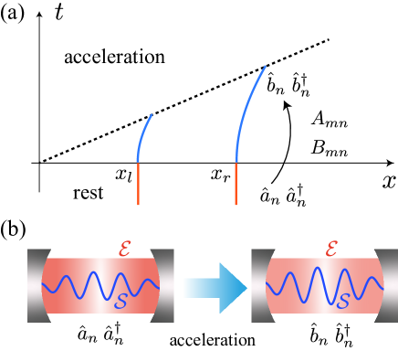
Figure 1: Illustration of relativistic quantum field in a cavity. (a) Example of cavity trajectory in Minkovski space. $x_{l}$ and $x_{r}$ are boundaries of the cavity, where $x_{r}-x_{l}=L>0$. The cavity is inertial for $t<0$ and starts to accelerate for $t\geq 0$. Due to the acceleration, the annihilation and creation operators undergoes the Bogoliubov transformation specified by $A_{mn}$ and $B_{mn}$. (b) Separation of system and environment. Modes specified by $\mathcal{S}$ correspond to the system and the remaining modes $\mathcal{E}$ relate to the environment.

Suppose that the cavity is in an inertial frame at the initial state. In relativistic quantum information, we are typically interested in only one or two modes in the cavity, whereas the remaining modes are regarded as the environment [9, 25]. Therefore, following Ref. [25], we divide all the modes into the system $\mathcal{S}$ and environment $\mathcal{E}$. A set of modes in the system $\mathcal{S}$ is defined as $\mathcal{S}=\{n_{s_{1}},n_{s_{2}},\ldots,n_{s_{K}}\}$, where $n_{s_{i}}\in\{1,2,\cdots\}$ denotes an index of the system mode satisfying $n_{s_{i}}\neq n_{s_{j}}$ for $i\neq j$, $K$ indicates the number of modes of the system, and a set of modes in the environment $\mathcal{E}$ comprises the remaining modes, i.e., $\mathcal{E}=\{n\in\{1,2,\cdots\}|n\notin\mathcal{S}\}$. Thus, a set of all the cavity modes can be expressed as $\mathcal{C}=\mathcal{E}\cup\mathcal{S}=\{1,2,\cdots\}$.

As the quantum field is an infinite-dimensional system, the thermodynamic quantities cannot be easily calculated. Thus, we employ the Gaussian state formalism [30, 31, 32] that is widely used in relativistic quantum information to compute thermodynamic quantities. Let $\hat{\xi}\equiv[\hat{a}_{1},\hat{a}_{2},...,\hat{a}_{1}^{\dagger},\hat{a}_{2}^{\dagger},...]^{\top}$. Subsequently, the covariance matrix $\sigma=\{\sigma_{mn}\}$ can be defined as

$$\sigma_{mn}\equiv\braket{\hat{\xi}_{m}\hat{\xi}_{n}^{\dagger}+\hat{\xi}_{n}^{\dagger}\hat{\xi}_{m}}-2\braket{\hat{\xi}_{m}}\braket{\hat{\xi}_{n}^{\dagger}},$$ (4)

where $\braket{\bullet}$ denotes the expectation value. Let $\sigma^{i}$ and $\sigma^{f}$ denote the covariance matrices before and after the coordinate transformation, respectively (hereinafter, variables with superscripts $i$ and $f$ indicate the stated aspect). In particular, the covariance matrix after Bogoliubov transformation can be expressed as

$$\sigma^{f}=\mathfrak{S}\sigma^{i}\mathfrak{S}^{\dagger},$$ (5)

where $\mathfrak{S}$ denotes a complex symplectic transformation, specified by the Bogoliubov matrices $A$ and $B$:

$$\mathfrak{S}=\left[\begin{array}[]{cc}A&B\\ B^{*}&A^{*}\end{array}\right].$$ (6)

The thermodynamic quantities of interest can be represented by the covariance matrix $\sigma$.

III Results

Let us consider a massless quantum field in a cavity that is initially in an inertial frame. According to the Klein–Goldon equation, the field mode $\phi_{n}$ ($n\in\{1,2,\cdots\}$) can be expressed as

$$\phi_{n}(t,x)=\frac{1}{\sqrt{n\pi}}\sin\left[\omega_{n}(x-x_{l})\right]e^{-i\omega_{n}t},$$ (7)

where we select a comoving frame $(t,x)$ with $x_{l}$ and $x_{r}$ as the cavity boundaries for any $t$ with $x_{r}-x_{l}=L>0$ (refer to Fig. 1(a)), and the Dirichlet boundary condition is imposed at the boundaries. The Hamiltonian operators of the system and environment are respectively defined as

$$\hat{H}_{\mathrm{sys}}\equiv\sum_{n\in\mathcal{S}}\omega_{n}\hat{a}_{n}^{\dagger}\hat{a}_{n},$$ (8)

$$\hat{H}_{\mathrm{env}}\equiv\sum_{n\in\mathcal{E}}\omega_{n}\hat{a}_{n}^{\dagger}\hat{a}_{n},$$ (9)

where $\omega_{n}\equiv\pi n/L$ denotes the angular frequency of the field mode. Let $\beta_{\mathrm{sys}}$ and $\beta_{\mathrm{env}}$ be the inverse temperature of the system and environment, respectively. We define the thermal states of the system and environment as follows:

$$\rho_{\mathrm{sys}}^{\mathrm{th}}(\beta_{\mathrm{sys}}) \equiv\frac{1}{Z_{\mathrm{sys}}(\beta_{\mathrm{sys}})}e^{-\beta_{\mathrm{sys}}\hat{H}_{\mathrm{sys}}},$$ (10)

$$\rho_{\mathrm{env}}^{\mathrm{th}}(\beta_{\mathrm{env}}) \equiv\frac{1}{Z_{\mathrm{env}}(\beta_{\mathrm{env}})}e^{-\beta_{\mathrm{env}}\hat{H}_{\mathrm{env}}},$$ (11)

where $Z_{\mathrm{sys}}(\beta_{\mathrm{sys}})$ and $Z_{\mathrm{env}}(\beta_{\mathrm{env}})$ are the partition functions defined as

$$Z_{\mathrm{sys}}(\beta_{\mathrm{env}}) \equiv\mathrm{Tr}_{\mathrm{sys}}[e^{-\beta_{\mathrm{env}}\hat{H}_{\mathrm{sys}}}],$$ (12)

$$Z_{\mathrm{env}}(\beta_{\mathrm{env}}) \equiv\mathrm{Tr}_{\mathrm{env}}[e^{-\beta_{\mathrm{env}}\hat{H}_{\mathrm{env}}}].$$ (13)

The initial density operator of the cavity is assumed to be $\rho_{\mathrm{cav}}^{i}=\rho_{\mathrm{sys}}^{i}\otimes\rho_{\mathrm{env}}^{i}$, where $\rho_{\mathrm{sys}}^{i}$ and $\rho_{\mathrm{env}}^{i}$ are given by $\rho_{\mathrm{sys}}^{i}=\rho_{\mathrm{sys}}^{\mathrm{th}}(\beta_{\mathrm{sys}}^{i})$ and $\rho_{\mathrm{env}}^{i}=\rho_{\mathrm{env}}^{\mathrm{th}}(\beta_{\mathrm{env}}^{i})$ with $\beta_{\mathrm{sys}}^{i}$ and $\beta_{\mathrm{env}}^{i}$ representing the initial inverse temperature of the system and environment, respectively. Let $\eta_{n}\equiv\mathrm{coth}(\beta_{\mathrm{sys}}^{i}\omega_{n}/2)$ and $\nu_{n}\equiv\mathrm{coth}(\beta_{\mathrm{env}}^{i}\omega_{n}/2)$ be the symplectic eigenvalues of the system and environment, respectively. The initial Gaussian states of the system and environment are respectively defined as

$$\sigma_{\mathrm{sys}}^{i} =\mathrm{diag}([\eta_{n}]_{n\in\mathcal{S}},[\eta_{n}]_{n\in\mathcal{S}}),$$ (14)

$$\sigma_{\mathrm{env}}^{i} =\mathrm{diag}([\nu_{n}]_{n\in\mathcal{E}},[\nu_{n}]_{n\in\mathcal{E}}).$$ (15)

Based on symplectic eigenvalues, the mean energy of the initial environment state can be derived as (refer to Appendix A)

$$\mathrm{Tr}_{\mathrm{env}}\left[\rho_{\mathrm{env}}^{i}\hat{H}_{\mathrm{env}}\right]=\sum_{n\in\mathcal{E}}\omega_{n}\frac{\sigma_{nn}^{i}-1}{2}.$$ (16)

Furthermore, the von Neumann entropy can be defined as

$$S_{\mathrm{sys}}(\rho_{\mathrm{sys}})\equiv-\mathrm{Tr}_{\mathrm{sys}}[\rho_{\mathrm{sys}}\ln\rho_{\mathrm{sys}}].$$ (17)

The von Neumann entropy is defined similarly for the environment $S_{\mathrm{env}}$ and cavity $S_{\mathrm{cav}}$. In the covariance matrix formalism, the von Neumann entropy can be represented by a symplectic eigenvalue of the system [33]:

$$S_{\mathrm{sys}}=\sum_{n\in\mathcal{S}}\left\{\mathfrak{s}_{+}\left(\eta_{n}\right)-\mathfrak{s}_{-}\left(\eta_{n}\right)\right\},$$ (18)

where $\mathfrak{s}_{\pm}(x)\equiv\left\{(x\pm 1)/2\right\}\ln\left\{(x\pm 1)/2\right\}$.

After preparing the initial state, the cavity undergoes arbitrary acceleration. An example of the trajectory for $t>0$ is exhibited in Fig. 1(a), where the cavity starts to accelerate satisfying the rigidity of the cavity. The coordinate transformation induced by the acceleration is modeled by the Bogoliubov transformation. Let $\hat{\zeta}\equiv[\hat{b}_{1},\hat{b}_{2},...,\hat{b}_{1}^{\dagger},\hat{b}_{2}^{\dagger},...]^{\top}$. The Bogoliubov transformation on operators $\hat{\xi}$ can be unitarily implemented as follows [34, 35, 30]:

$$\hat{\zeta}=\mathfrak{S}\hat{\xi}=\hat{U}^{\dagger}(\mathfrak{S})\hat{\xi}\hat{U}(\mathfrak{S}),$$ (19)

where $\mathfrak{S}$ denotes a symplectic transformation defined as Eq. (6) and $\hat{U}(\mathfrak{S})$ denotes a unitary operator satisfying $\hat{U}(\mathfrak{S}_{1}\mathfrak{S}_{2})=\hat{U}(\mathfrak{S}_{1})\hat{U}(\mathfrak{S}_{2})$. Equation (19) is the Heisenberg picture of the creation and annihilation operators. Therefore, in the Schrödinger picture, the density operator of the entire cavity evolves unitarily as $\rho_{\mathrm{cav}}^{f}=\hat{U}(\mathfrak{S})\rho_{\mathrm{cav}}^{i}\hat{U}^{\dagger}(\mathfrak{S})$. In the quantum thermodynamics, the dissipated heat is often defined by the energy difference in the environment between the final and initial states:

$$\Delta Q \equiv\mathrm{Tr}_{\mathrm{env}}[\rho_{\mathrm{env}}^{f}\hat{H}_{\mathrm{env}}]-\mathrm{Tr}_{\mathrm{env}}[\rho_{\mathrm{env}}^{i}\hat{H}_{\mathrm{env}}]$$

$$=\sum_{n\in\mathcal{E}}\omega_{n}\frac{\sigma_{nn}^{f}-\sigma_{nn}^{i}}{2},$$ (20)

where $\rho_{\mathrm{env}}^{f}\equiv\mathrm{Tr}_{\mathrm{sys}}[\rho_{\mathrm{cav}}^{f}]=\mathrm{Tr}_{\mathrm{sys}}[\hat{U}\rho_{\mathrm{cav}}^{i}\hat{U}^{\dagger}]$ denotes the final density operator of the environment. The entropy difference between the initial and final states can be expressed as

$$\Delta S_{\mathrm{sys}}\equiv S_{\mathrm{sys}}(\rho_{\mathrm{sys}}^{f})-S_{\mathrm{sys}}(\rho_{\mathrm{sys}}^{i}),$$ (21)

where the covariance matrix representation of $S_{\mathrm{sys}}$ follows that in Eq. (18).

Subsequently, we define the entropy production for a quantum field in a cavity. The entropy production plays fundamental roles in stochastic and quantum thermodynamics, which can be defined following several manner [36, 26]. For instance, in stochastic thermodynamics, the entropy production can be quantified by the probability ratio between the forward and backward processes, or it may be defined by a total entropy that includes both the system and environment. In the quantum domain, owing to the high degree of freedom in modeling, the entropy production can be defined following several mechanisms [26]. Here, we define the entropy production as

$$\Sigma\equiv\beta_{\mathrm{env}}^{i}\Delta Q+\Delta S_{\mathrm{sys}},$$ (22)

which denotes the sum of the dissipated heat [Eq. (20)] and the von Neumann entropy of the system [Eq. (21)]. As the modes in the cavity undergo Bogoliubov transformation, the density operator of the entire cavity $\rho_{\mathrm{cav}}$ evolves via the corresponding unitary operator [Eq. (19)]. Therefore, from Refs. [37, 38], the following relation holds (refer to Appendix B):

$$\Sigma=I+D(\rho_{\mathrm{env}}^{f}||\rho_{\mathrm{env}}^{i})\geq D(\rho_{\mathrm{env}}^{f}||\rho_{\mathrm{env}}^{i})\geq 0,$$ (23)

where $D(\rho_{\mathrm{env}}^{f}||\rho_{\mathrm{env}}^{i})$ and $I$ are the quantum relative entropy and the quantum mutual information, respectively, defined by

$$D(\rho_{\mathrm{env}}^{f}||\rho_{\mathrm{env}}^{i}) \equiv\mathrm{Tr}_{\mathrm{env}}\left[\rho_{\mathrm{env}}^{f}\ln\rho_{\mathrm{env}}^{f}\right]-\mathrm{Tr}_{\mathrm{env}}\left[\rho_{\mathrm{env}}^{f}\ln\rho_{\mathrm{env}}^{i}\right],$$ (24)

$$I \equiv S_{\mathrm{sys}}(\rho_{\mathrm{sys}}^{f})+S_{\mathrm{env}}(\rho_{\mathrm{env}}^{f})-S_{\mathrm{cav}}(\rho_{\mathrm{cav}}^{f}).$$ (25)

The quantum relative entropy and quantum mutual information are nonnegative [39] (nonnegativity of quantum mutual information used in the second line of Eq. (23)). As expressed in Eq. (23), the entropy production is nonnegative, $\Sigma\geq 0$, under a coordinate transformation induced by the acceleration, which is a second law of thermodynamics for a quantum field in a cavity.

Prior to delving into deeper analysis of the entropy production $\Sigma$, we explain certain aspects. In this study, we defined heat as the variation in the energy of the environment. Heat is induced by the interaction between the system and environment. Although the exchange of energy between the system and environment is identified as heat in classical thermodynamics, the distinction of heat from work in the quantum setting is often nontrivial. Prior studies have attempted to define heat and work in quantum thermodynamics, which can be primarily classified into two fundamental definitions, namely, heat-first and work-first definitions [40]. In the heat-first definition, heat is defined as the variation in the energy of the environment [41]. This definition is commonly applied to the two-point measurement scheme [42], where projective measurement with respect to the environmental energy eigenbasis is performed at the beginning and end of the process, and the heat is defined as the difference between them. In the second category, work is defined first, which was initially proposed in Ref [43]. This study employed the heat-first definition.

The first term in Eq. (22) represents the increase in environmental entropy, which is true for the ideal environment that maintains its equilibrium and with constant temperature during the evolution. However, the definition of temperature in general nonequilibrium states persists to be a challenge [44]. Therefore, in the standard quantum thermodynamics, the entropy production in Eq. (22) is defined as the entropy production for an arbitrary environment [26]. This is because $\Sigma$ defined in Eq. (22) is positive in all cases, consistent with the most essential requirement for entropy production. Moreover, the definition of Eq. (22) is consistent with that of classical thermodynamics. Note that the entropy production in Eq. (22) exhibits the operational meaning in case of considering a fluctuation theorem [45], which is the fundamental equality in nonequilibrium thermodynamics.

This study focuses on heat but not on work, which constitutes the counterpart quantity in thermodynamics. As the unitary $\hat{U}(\mathfrak{S})$ in Eq. (19) implicitly includes the contribution of work, the variation in energy of the system is not equal to the heat, $\Delta H_{\mathrm{sys}}+\Delta Q\neq 0$ [26], where $\Delta H_{\mathrm{sys}}$ represents the variations in the system energy:

$$\Delta H_{\mathrm{sys}} \equiv\mathrm{Tr}_{\mathrm{sys}}\left[\rho_{\mathrm{sys}}^{f}\hat{H}_{\mathrm{sys}}\right]-\mathrm{Tr}_{\mathrm{sys}}\left[\rho_{\mathrm{sys}}^{i}\hat{H}_{\mathrm{sys}}\right]$$

$$=\sum_{n\in\mathcal{S}}\frac{\sigma_{nn}^{f}-\sigma_{nn}^{i}}{2}.$$ (26)

According to the first law, the exerted work can be defined as the difference between $\Delta\hat{H}_{\mathrm{sys}}$ and $\Delta Q$:

$$\Delta W\equiv\Delta H_{\mathrm{sys}}+\Delta Q.$$ (27)

Based on the work defined in Eq. (27), the entropy production of Eq. (22) can be represented as

$$\Sigma=\beta_{\mathrm{env}}^{i}\left(\Delta W-\Delta F\right),$$ (28)

where $\Delta F\equiv F(\rho_{\mathrm{sys}}^{f})-F(\rho_{\mathrm{sys}}^{i})$ represents the variation in free energy, and $F(\rho_{\mathrm{sys}})$ indicates the free energy defined as

$$F(\rho_{\mathrm{sys}})\equiv\mathrm{Tr}_{\mathrm{sys}}[\hat{H}_{\mathrm{sys}}\rho_{\mathrm{sys}}]-\frac{1}{\beta_{\mathrm{env}}^{i}}S_{\mathrm{sys}}(\rho_{\mathrm{sys}}).$$ (29)

The second law $\Sigma\geq 0$ yields $\Delta W\geq\Delta F$, which states that the work exerted on the system is greater than or equal to the free energy difference, which is consistent with another classical definition of entropy production.

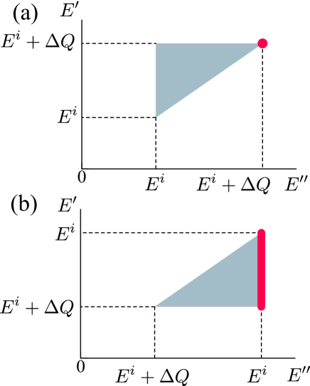
Figure 2: Integral regions of Eq. (34) for (a) $\Delta Q>0$ and (b) $\Delta Q<0$. Pink regions denote values of $E^{\prime\prime}$ and $E^{\prime}$ at which $\mathrm{Var}_{\beta}[\hat{H}_{\mathrm{env}}]$ gives the maximum.

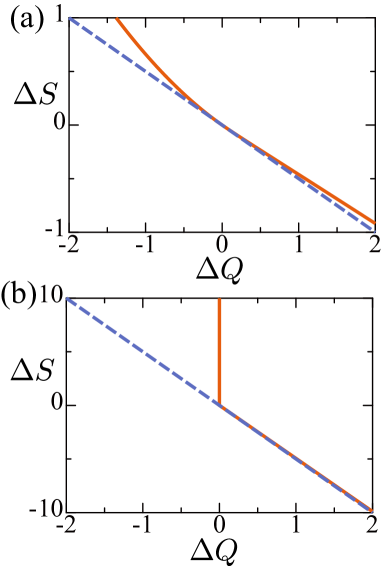
Figure 3: Region plot of lower bound [Eq. (36)] for cavity with (a) $\beta_{\mathrm{env}}^{i}=0.5$ and (b) $\beta_{\mathrm{env}}^{i}=5.0$. The solid line represents Eq. (36) and the dashed line denotes $\Delta S_{\mathrm{sys}}\geq-\beta_{\mathrm{env}}^{i}\Delta Q$. The regions above the solid lines are physically feasible, whereas the other settings are $\mathcal{S}=\{1\}$ and $L=1$.

We can refine Eq. (23) by using the fact that the environment comprises a bosonic quantum field. To calculate the lower bound of $D(\rho_{\mathrm{env}}^{f}||\rho_{\mathrm{env}}^{i})$, we follow Ref. [38]. According to the Pythagoras relation [38] that can be proved by simple calculations, $D(\rho_{\mathrm{env}}^{f}||\rho_{\mathrm{env}}^{i})$ is bounded from below by

$$D(\rho_{\mathrm{env}}^{f}||\rho_{\mathrm{env}}^{i}) =D(\rho_{\mathrm{env}}^{f}||\rho_{\mathrm{env}}^{\mathrm{th},f})+D(\rho_{\mathrm{env}}^{\mathrm{th},f}||\rho_{\mathrm{env}}^{i})$$

$$\geq D(\rho_{\mathrm{env}}^{\mathrm{th},f}||\rho_{\mathrm{env}}^{i}),$$ (30)

where $\rho_{\mathrm{env}}^{\mathrm{th},f}$ denotes a thermal state that yields the same energy as $\rho_{\mathrm{env}}^{f}$. Let $E(\beta_{\mathrm{env}})$ be the mean energy of the environment with respect to a thermal state with the inverse temperature $\beta_{\mathrm{env}}$:

$$E(\beta_{\mathrm{env}})\equiv\mathrm{Tr}_{\mathrm{env}}\left[\rho_{\mathrm{env}}^{\mathrm{th}}(\beta_{\mathrm{env}})\hat{H}_{\mathrm{env}}\right].$$ (31)

Thereafter, we obtain

$$E^{i}+\Delta Q=\mathrm{Tr}_{\mathrm{env}}[\rho_{\mathrm{env}}^{f}\hat{H}_{\mathrm{env}}]=\mathrm{Tr}_{\mathrm{env}}[\rho_{\mathrm{env}}^{\mathrm{th},f}\hat{H}_{\mathrm{env}}],$$ (32)

where $E^{i}\equiv E(\beta_{\mathrm{env}}^{i})=\mathrm{Tr}_{\mathrm{env}}[\rho_{\mathrm{env}}^{i}\hat{H}_{\mathrm{env}}]$. As $(d/d\beta_{\mathrm{env}})E(\beta_{\mathrm{env}})<0$, $\beta_{\mathrm{env}}^{\mathrm{th},f}$ satisfies $E(\beta_{\mathrm{env}}^{\mathrm{th},f})=E^{i}+\Delta Q$ and can be uniquely specified given $\Delta Q$. Therefore, given $\Delta Q$, $\rho_{\mathrm{env}}^{\mathrm{th},f}=\rho_{\mathrm{env}}^{\mathrm{th}}(\beta_{\mathrm{env}}^{\mathrm{th},f})$ can be uniquely identified, indicating that $D(\rho_{\mathrm{env}}^{\mathrm{th},f}||\rho_{\mathrm{env}}^{i})$ in Eq. (30) can be calculated with $\Delta Q$. The relative entropy admits the following expression:

$$D(\rho_{\mathrm{env}}^{\mathrm{th},f}||\rho_{\mathrm{env}}^{i})=\beta_{\mathrm{env}}^{i}\Delta Q-\left[S_{\mathrm{env}}(\rho_{\mathrm{env}}^{\mathrm{th},f})-S_{\mathrm{env}}(\rho_{\mathrm{env}}^{i})\right].$$ (33)

Based on Ref. [38], $D(\rho_{\mathrm{env}}^{\mathrm{th},f}||\rho_{\mathrm{env}}^{i})$ in Eq. (33) can be rewritten as (refer to Appendix C):

$$D(\rho_{\mathrm{env}}^{\mathrm{th},f}||\rho_{\mathrm{env}}^{i})=\int_{E^{i}}^{E^{i}+\Delta Q}dE^{\prime}\int_{E^{i}}^{E^{\prime}}\frac{dE^{\prime\prime}}{\mathrm{Var}_{\beta_{\mathrm{env}}(E^{\prime\prime})}[\hat{H}_{\mathrm{env}}]},$$ (34)

where $\mathrm{Var}_{\beta_{\mathrm{env}}}[\hat{H}_{\mathrm{env}}]$ denotes the variance of $\hat{H}_{\mathrm{env}}$ with respect to the thermal state of the environment with inverse temperature $\beta_{\mathrm{env}}$:

$$\mathrm{Var}_{\beta_{\mathrm{env}}}[\hat{H}_{\mathrm{env}}]=\frac{1}{4}\sum_{n\in\mathcal{E}}\omega_{n}^{2}\mathrm{csch}\left(\frac{\beta_{\mathrm{env}}\omega_{n}}{2}\right)^{2},$$ (35)

where $\beta_{\mathrm{env}}(E)$ denotes the inverse temperature $\beta_{\mathrm{env}}$, satisfying $E=\mathrm{Tr}_{\mathrm{env}}\left[\rho_{\mathrm{env}}^{\mathrm{th}}(\beta_{\mathrm{env}})\hat{H}_{\mathrm{env}}\right]$, which can be uniquely identified because $E(\beta_{\mathrm{env}})$ is a monotonically decreasing function. Thereafter, we calculate the maximum value of $\mathrm{Var}_{\beta_{\mathrm{env}}}[\hat{H}_{\mathrm{env}}]$ within the integral domain $\int_{E^{i}}^{E^{i}+\Delta Q}dE^{\prime}\int_{E^{i}}^{E^{\prime}}dE^{\prime\prime}$. Specifically, we need to separately consider the two cases of $\Delta Q>0$ and $\Delta Q<0$. As $\beta_{\mathrm{env}}(E)$ is a monotonically decreasing function of $E$, $\mathrm{Var}_{\beta_{\mathrm{env}}}[\hat{H}_{\mathrm{env}}]$ provides the maximum value for $\Delta Q>0$ and $\Delta Q<0$ at the points indicated in Fig. 2(a) and (b), respectively. Considering the maximum, we derive a refined version of the second law for the accelerated cavities as follows:

$$\Delta S_{\mathrm{sys}}+\beta_{\mathrm{env}}^{i}\Delta Q\geq\begin{cases}{\displaystyle\frac{(\Delta Q)^{2}}{2\mathrm{Var}_{\beta_{\mathrm{env}}^{i}}[\hat{H}_{\mathrm{env}}]}}&\Delta Q\leq 0\\ {\displaystyle\frac{(\Delta Q)^{2}}{2\mathrm{Var}_{\beta_{\mathrm{env}}(E^{i}+\Delta Q)}[\hat{H}_{\mathrm{env}}]}}&\Delta Q>0\end{cases},$$ (36)

which forms the main result of this research. In Eq. (36), the variance term for $\Delta Q<0$ does not rely on $\Delta Q$, unlike $\Delta Q>0$. Equation (36) holds for an arbitrary Bogoliubov transformation, indicating that Eq. (36) should hold for any acceleration undergone by the cavity. Equation (36) is a refined version of the second law for the quantum field in the cavity. Although the above calculation follows Ref. [38], the lower bound of Eq. (36) differs from that reported in Ref. [38] because the cavity is an infinite-dimensional system, whereas Ref. [38] concerns finite-dimensional systems.

Although Eq. (36) represents the statement for entropy production, it can be regarded as a statement between the variation in information in the system and the energy dissipated in the environment, i.e., Eq. (36) can be identified as the Landauer principle for a quantum field in the cavity undergoing acceleration. The Landauer principle concerns the entropy decrease in the system, quantified by $-\Delta S_{\mathrm{sys}}$, and yields the lower bound of the heat dissipation to realize the entropy decrease. Equation (36) is plotted in Fig. 3 with the solid lines for two inverse temperature settings in (a) $\beta_{\mathrm{env}}^{i}=0.5$ and (b) $\beta_{\mathrm{env}}^{i}=5.0$ (explicit parameters are stated in the caption). The regions above the solid lines denote the feasible regions predicted by Eq. (36). In Fig. 3, the dashed lines represent the lower bound of $\Sigma=\Delta S_{\mathrm{sys}}+\beta_{\mathrm{env}}^{i}\Delta Q\geq 0$, which represents the naive second law. As observed, the area of the negative heat region diminishes with the temperature. More importantly, Eq. (36) is tighter than the naive second law under high temperature.

Another consequence of Eq. (36) pertains to its relation with information scrambling [46, 47]. Generally, the extent of scrambling is quantified by out-of-order correlators. As proposed earlier, the extent of scrambling can alternatively be quantified by quantum mutual information [48]. The cavity undergoing a nonuniform acceleration can be identified as a process of information spreading. Suppose that the cavity contains modes only in $\mathcal{S}$ and the remaining modes are vacant. After acceleration, the other remaining modes are populated because of the Bogoliubov transformation, which is a reminiscent of the scrambling process. The mutual information $I$ is bounded from above by $I\leq\Delta S_{\mathrm{sys}}+\beta_{\mathrm{env}}^{i}\Delta Q-D(\rho_{\mathrm{env}}^{\mathrm{th},f}||\rho_{\mathrm{env}}^{i})$. Based on Eq. (36), we obtain

$$I\leq\begin{cases}\beta_{\mathrm{env}}^{i}\Delta Q+\Delta S_{\mathrm{sys}}-{\displaystyle\frac{(\Delta Q)^{2}}{2\mathrm{Var}_{\beta_{\mathrm{env}}^{i}}[\hat{H}_{\mathrm{env}}]}}&\Delta Q\leq 0\\ \beta_{\mathrm{env}}^{i}\Delta Q+\Delta S_{\mathrm{sys}}-{\displaystyle\frac{(\Delta Q)^{2}}{2\mathrm{Var}_{\beta_{\mathrm{env}}(E^{i}+\Delta Q)}[\hat{H}_{\mathrm{env}}]}}&\Delta Q>0\end{cases},$$ (37)

which indicates that the degree of scrambling induced by the acceleration of the cavity can be upper-bounded by the entropy $\Delta S_{\mathrm{sys}}$ and dissipated heat $\Delta Q$ in the cavity.

IV Conclusion

In this paper, we obtained the lower bound for the entropy production of a quantum field in a cavity undergoing acceleration. First, the cavity mode of interest was regarded as the system and the remaining modes as the environment. Thereafter, the entropy production was defined as the sum of the von Neumann entropy of the system and the dissipated heat. The nonnegativity of the entropy production is a signature of the second law and provides the statement of the Landauer principle for the accelerated cavity.

Appendix A Quantities of quantum field

For readers’ convenience, we review the quantities of quantum fields in a general setting. Let us consider the thermal state of the Hamiltonian $\hat{H}=\sum_{n}\omega_{n}\hat{a}_{n}^{\dagger}\hat{a}_{n}$. The density operator can be expressed as

$$\rho^{\mathrm{th}}\equiv\frac{1}{Z(\beta)}e^{-\beta\hat{H}},$$ (38)

where $\beta$ denotes the inverse temperature and $Z(\beta)\equiv\mathrm{Tr}[e^{-\beta\hat{H}}]$. The number operator $\hat{\mathfrak{n}}_{n}\equiv\hat{a}_{n}^{\dagger}\hat{a}_{n}$ admits the eigendecomposition

$$\hat{\mathfrak{n}}_{n}\ket{\mathfrak{n}_{n}}=\mathfrak{n}_{n}\ket{\mathfrak{n}_{n}},$$ (39)

which implies that $\hat{\mathfrak{n}}_{n}$ can be represented as $\hat{\mathfrak{n}}_{n}=\sum_{\mathfrak{n}_{n}}{\mathfrak{n}}_{n}\ket{\mathfrak{n}_{n}}\bra{\mathfrak{n}_{n}}$. Based on this representation, the terms in $\rho^{\mathrm{th}}$ can be expressed as

$$e^{-\beta\hat{H}}=\prod_{n=1}^{\infty}e^{-\beta\omega_{n}\hat{\mathfrak{n}}_{n}}=\prod_{n=1}^{\infty}\sum_{\mathfrak{n}_{n}}e^{-\beta\omega_{n}\mathfrak{n}_{n}}\ket{\mathfrak{n}_{n}}\bra{\mathfrak{n}_{n}},$$ (40)

and

$$\mathrm{Tr}[e^{-\beta\hat{H}}]=\prod_{n}\left(\sum_{\mathfrak{n}_{n}}e^{-\beta\omega_{n}\mathfrak{n}_{n}}\right)=\prod_{n}\frac{e^{\beta\omega_{n}}}{e^{\beta\omega_{n}}-1}.$$ (41)

Let us consider the expectation of $\hat{a}_{n}^{\dagger}\hat{a}_{n}$ with respect to the thermal state $\rho^{\mathrm{th}}$:

$$\braket{\hat{a}_{n}^{\dagger}\hat{a}_{n}}=\mathrm{Tr}\left[\hat{\mathfrak{n}}_{n}\rho^{\mathrm{th}}\right]=\frac{\sum_{\mathfrak{n}_{n}}\mathfrak{n}_{n}e^{-\beta\omega_{n}\mathfrak{n}_{n}}}{\sum_{\mathfrak{n}_{n}}e^{-\beta\omega_{n}\mathfrak{n}_{n}}}=\frac{1}{e^{\beta\omega_{n}}-1}.$$ (42)

As $\sigma_{nn}=\braket{\hat{a}_{n}^{\dagger}\hat{a}_{n}+\hat{a}_{n}\hat{a}_{n}^{\dagger}}=2\braket{\hat{a}_{n}^{\dagger}\hat{a}_{n}}+1$, the covariance matrix becomes

$$\sigma_{nn}=2\braket{\hat{a}_{n}^{\dagger}\hat{a}_{n}}+1=\mathrm{coth}\left(\frac{\beta\omega_{n}}{2}\right).$$ (43)

According to Eq. (42), the mean of $\hat{H}$ can be derived as

$$\mathrm{Tr}[\rho^{\mathrm{th}}\hat{H}]=\sum_{n}\frac{\omega_{n}}{e^{\beta\omega_{n}}-1}.$$ (44)

Similarly, the second moment of $\hat{H}$ can be evaluated as

$$\mathrm{Tr}\left[\rho^{\mathrm{th}}\hat{H}^{2}\right] =\sum_{n}\frac{(e^{\beta\omega_{n}}+1)\omega_{n}^{2}}{(e^{\beta\omega_{n}}-1)^{2}}$$

$$+\sum_{n\neq m}\left(\frac{\omega_{n}}{e^{\beta\omega_{n}}-1}\right)\left(\frac{\omega_{m}}{e^{\beta\omega_{m}}-1}\right).$$ (45)

Using Eqs. (44) and (45), the variance of $\hat{H}$ is expressed as

$$\mathrm{Var}[\hat{H}] =\mathrm{Tr}\left[\rho^{\mathrm{th}}\hat{H}^{2}\right]-\mathrm{Tr}\left[\rho^{\mathrm{th}}\hat{H}\right]^{2}$$

$$=\sum_{n}\frac{e^{\beta\omega_{n}}\omega_{n}^{2}}{(e^{\beta\omega_{n}}-1)^{2}}$$

$$=\frac{1}{4}\sum_{n}\omega_{n}^{2}\mathrm{csch}\left(\frac{\beta\omega_{n}}{2}\right)^{2},$$ (46)

where $\mathrm{csch}(x)\equiv 1/\sinh(x)$.

$E(\beta)$ is defined in Eq. (31) with a derivative of

$$\frac{d}{d\beta}E(\beta)=-\sum_{n\in\mathcal{E}}\frac{e^{\beta\omega_{n}}\omega_{n}^{2}}{(e^{\beta\omega_{n}}-1)^{2}}<0.$$ (47)

The above equation establishes the definition of the inverse function $\beta(E)$.

Appendix B Derivation of Eq. (23)

The derivation of Eq. (23) is presented herein, which has been proved in Refs. [37, 38]. We will express the following relation:

$$\beta_{\mathrm{env}}^{i}\Delta Q+\Delta S_{\mathrm{sys}}=I+D(\rho_{\mathrm{env}}^{f}||\rho_{\mathrm{env}}^{i}).$$ (48)

As discussed in the main text, the entire cavity undergoes a unitary transformation: $\rho_{\mathrm{cav}}^{f}=U\rho_{\mathrm{cav}}^{i}U^{\dagger}$. Therefore, the von Neumann entropy of the entire cavity is invariant under the transformation: $S_{\mathrm{cav}}(\rho_{\mathrm{cav}}^{f})=S_{\mathrm{cav}}(\rho_{\mathrm{cav}}^{i})=S_{\mathrm{sys}}(\rho_{\mathrm{sys}}^{i})+S_{\mathrm{env}}(\rho_{\mathrm{env}}^{i})$, where we considered that the state is initially in a product state in the last equality. Therefore, we obtain

$$I+D(\rho_{\mathrm{env}}^{f}||\rho_{\mathrm{env}}^{i})=\Delta S+\mathrm{Tr}_{\mathrm{env}}\left[(\rho_{\mathrm{env}}^{i}-\rho_{\mathrm{env}}^{f})\ln\rho_{\mathrm{env}}^{i}\right].$$ (49)

As $\rho_{\mathrm{env}}^{i}=Z_{\mathrm{env}}(\beta_{\mathrm{env}}^{i})^{-1}e^{-\beta_{\mathrm{env}}^{i}\hat{H}_{\mathrm{env}}}$, the second term in Eq. (49) can be rewritten as

$$\mathrm{Tr}_{\mathrm{env}}\left[(\rho_{\mathrm{env}}^{i}-\rho_{\mathrm{env}}^{f})\ln\rho_{\mathrm{env}}^{i}\right]$$

$$=\mathrm{Tr}_{\mathrm{env}}\left[(\rho_{\mathrm{env}}^{i}-\rho_{\mathrm{env}}^{f})(-\beta_{\mathrm{env}}^{i}\hat{H}_{\mathrm{env}})\right]$$

$$=\beta_{\mathrm{env}}^{i}\Delta Q.$$ (50)

Equation (23) directly follows from Eqs. (49) and (50).

Appendix C Derivation of Eq. (34)

Herein, we derive Eq. (34) based on Refs. [38]:

$$D(\rho_{\mathrm{env}}^{\mathrm{th},f}||\rho_{\mathrm{env}}^{i}) =\beta_{\mathrm{env}}^{i}\Delta Q-\int_{E^{i}}^{E^{i}+\Delta Q}\frac{dS_{\mathrm{env}}^{\mathrm{th}}(\beta_{\mathrm{env}}(E^{\prime}))}{dE^{\prime}}dE^{\prime}$$

$$=\beta_{\mathrm{env}}^{i}\Delta Q-\int_{E^{i}}^{E^{i}+\Delta Q}\beta_{\mathrm{env}}(E^{\prime})dE^{\prime}$$

$$=\int_{E^{i}}^{E^{i}+\Delta Q}\left(\beta_{\mathrm{env}}^{i}-\beta_{\mathrm{env}}(E^{\prime})\right)dE^{\prime}$$

$$=\int_{E^{i}}^{E^{i}+\Delta Q}dE^{\prime}\int_{E^{\prime}}^{E^{i}}\frac{d\beta_{\mathrm{env}}(E^{\prime\prime})}{dE^{\prime\prime}}dE^{\prime\prime}$$

$$=\int_{E^{i}}^{E^{i}+\Delta Q}dE^{\prime}\int_{E^{i}}^{E^{\prime}}\frac{dE^{\prime\prime}}{\mathrm{Var}_{\beta_{\mathrm{env}}(E^{\prime\prime})}[\hat{H}_{\mathrm{env}}]},$$ (51)

where $S_{\mathrm{env}}^{\mathrm{th}}(\beta_{\mathrm{env}})$ is defined as

$$S_{\mathrm{env}}^{\mathrm{th}}(\beta_{\mathrm{env}})\equiv-\mathrm{Tr}_{\mathrm{env}}\left[\rho_{\mathrm{env}}^{\mathrm{th}}(\beta_{\mathrm{env}})\ln\rho_{\mathrm{env}}^{\mathrm{th}}(\beta_{\mathrm{env}})\right].$$ (52)

When calculating Eq. (51), we used the following relations:

$$\frac{d\beta_{\mathrm{env}}}{dE} =\frac{1}{dE/d\beta_{\mathrm{env}}}=-\frac{1}{\mathrm{Var}_{\beta_{\mathrm{env}}(E)}[\hat{H}_{\mathrm{env}}]},$$ (53)

$$\frac{d\rho_{\mathrm{env}}^{\mathrm{th}}(\beta_{\mathrm{env}})}{d\beta_{\mathrm{env}}} =-\hat{H}_{\mathrm{env}}\rho_{\mathrm{env}}^{\mathrm{th}}(\beta_{\mathrm{env}})$$

$$+\rho_{\mathrm{env}}^{\mathrm{th}}(\beta_{\mathrm{env}})\mathrm{Tr}_{\mathrm{env}}\left[\rho_{\mathrm{env}}^{\mathrm{th}}(\beta_{\mathrm{env}})\hat{H}_{\mathrm{env}}\right],$$ (54)

$$\frac{dS_{\mathrm{env}}^{\mathrm{th}}}{d\beta_{\mathrm{env}}} =-\mathrm{Tr}_{\mathrm{env}}\left[\frac{d\rho_{\mathrm{env}}^{\mathrm{th}}(\beta_{\mathrm{env}})}{d\beta_{\mathrm{env}}}\ln\rho_{\mathrm{env}}^{\mathrm{th}}(\beta_{\mathrm{env}})\right]$$

$$=-\beta_{\mathrm{env}}\mathrm{Var}_{\beta_{\mathrm{env}}}\left[\hat{H}_{\mathrm{env}}\right],$$ (55)

$$\frac{dS_{\mathrm{env}}^{\mathrm{th}}(\beta_{\mathrm{env}}(E))}{dE} =\frac{dS_{\mathrm{env}}^{\mathrm{th}}(\beta_{\mathrm{env}})}{d\beta_{\mathrm{env}}}\frac{d\beta_{\mathrm{env}}}{dE}=\beta_{\mathrm{env}}(E).$$ (56)

References

- Hawking [1974] S. W. Hawking, Black hole explosions?, Nature 248, 30 (1974).
- Crispino et al. [2008] L. C. B. Crispino, A. Higuchi, and G. E. A. Matsas, The Unruh effect and its applications, Rev. Mod. Phys. 80, 787 (2008).
- Mann and Ralph [2012] R. B. Mann and T. C. Ralph, Relativistic quantum information, Classical Quantum Gravity 29, 220301 (2012).
- Peres and Terno [2004] A. Peres and D. R. Terno, Quantum information and relativity theory, Rev. Mod. Phys. 76, 93 (2004).
- Yin et al. [2017] J. Yin et al., Satellite-based entanglement distribution over 1200 kilometers, Science 356, 1140 (2017).
- Dodonov [2010] V. V. Dodonov, Current status of the dynamical Casimir effect, Physica Scripta 82, 038105 (2010).
- Fuentes-Schuller and Mann [2005] I. Fuentes-Schuller and R. B. Mann, Alice falls into a black hole: Entanglement in noninertial frames, Phys. Rev. Lett. 95, 120404 (2005).
- Downes et al. [2011] T. G. Downes, I. Fuentes, and T. C. Ralph, Entangling moving cavities in noninertial frames, Phys. Rev. Lett. 106, 210502 (2011).
- Bruschi et al. [2012] D. E. Bruschi, I. Fuentes, and J. Louko, Voyage to Alpha Centauri: Entanglement degradation of cavity modes due to motion, Phys. Rev. D 85, 061701 (2012).
- Martín-Martínez et al. [2013] E. Martín-Martínez, D. Aasen, and A. Kempf, Processing quantum information with relativistic motion of atoms, Phys. Rev. Lett. 110, 160501 (2013).
- Bruschi et al. [2013] D. E. Bruschi, A. Dragan, A. R. Lee, I. Fuentes, and J. Louko, Relativistic motion generates quantum gates and entanglement resonances, Phys. Rev. Lett. 111, 090504 (2013).
- Ahmadi et al. [2014] M. Ahmadi, D. E. Bruschi, C. Sabín, G. Adesso, and I. Fuentes, Relativistic quantum metrology: Exploiting relativity to improve quantum measurement technologies, Sci. Rep. 4, 4996 (2014).
- Jarzynski [1997] C. Jarzynski, Nonequilibrium equality for free energy differences, Phys. Rev. Lett. 78, 2690 (1997).
- Evans et al. [1993] D. J. Evans, E. G. D. Cohen, and G. P. Morriss, Probability of second law violations in shearing steady states, Phys. Rev. Lett. 71, 2401 (1993).
- Gallavotti and Cohen [1995] G. Gallavotti and E. G. D. Cohen, Dynamical ensembles in nonequilibrium statistical mechanics, Phys. Rev. Lett. 74 (1995).
- Crooks [1999] G. E. Crooks, Entropy production fluctuation theorem and the nonequilibrium work relation for free energy differences, Phys. Rev. E 60, 2721 (1999).
- Barato and Seifert [2015] A. C. Barato and U. Seifert, Thermodynamic uncertainty relation for biomolecular processes, Phys. Rev. Lett. 114, 158101 (2015).
- Horowitz and Gingrich [2019] J. M. Horowitz and T. R. Gingrich, Thermodynamic uncertainty relations constrain non-equilibrium fluctuations, Nat. Phys. (2019).
- Mukamel [2003] S. Mukamel, Quantum extension of the Jarzynski relation: Analogy with stochastic dephasing, Phys. Rev. Lett. 90, 170604 (2003).
- Funo et al. [2018] K. Funo, M. Ueda, and T. Sagawa, Quantum fluctuation theorems, in Thermodynamics in the Quantum Regime: Fundamental Aspects and New Directions, edited by F. Binder, L. A. Correa, C. Gogolin, J. Anders, and G. Adesso (Springer International Publishing, 2018) pp. 249–273.
- Hasegawa [2021] Y. Hasegawa, Thermodynamic uncertainty relation for general open quantum systems, Phys. Rev. Lett. 126, 010602 (2021).
- Bartolotta and Deffner [2018] A. Bartolotta and S. Deffner, Jarzynski equality for driven quantum field theories, Phys. Rev. X 8, 011033 (2018).
- Ortega et al. [2019] A. Ortega, E. McKay, A. M. Alhambra, and E. Martín-Martínez, Work distributions on quantum fields, Phys. Rev. Lett. 122, 240604 (2019).
- Liu et al. [2016] N. Liu, J. Goold, I. Fuentes, V. Vedral, K. Modi, and D. E. Bruschi, Quantum thermodynamics for a model of an expanding universe, Classical and Quantum Gravity 33, 035003 (2016).
- Bruschi et al. [2020] D. E. Bruschi, B. Morris, and I. Fuentes, Thermodynamics of relativistic quantum fields confined in cavities, Phys. Lett. A 384, 126601 (2020).
- Landi and Paternostro [2021] G. T. Landi and M. Paternostro, Irreversible entropy production: From classical to quantum, Rev. Mod. Phys. 93, 035008 (2021).
- Landauer [1961] R. Landauer, Irreversibility and heat generation in the computing process, IBM Journal of Research and Development 5, 183 (1961).
- Friis [2013] N. Friis, Cavity mode entanglement in relativistic quantum information, arXiv:1311.3536 (2013).
- Mukhanov and Winitzki [2007] V. Mukhanov and S. Winitzki, Introduction to quantum effects in gravity (Cambridge university press, 2007).
- Ferraro et al. [2005] A. Ferraro, S. Olivares, and M. G. A. Paris, Gaussian states in continuous variable quantum information (Bibliopolis, 2005).
- Wang et al. [2007] X.-B. Wang, T. Hiroshima, A. Tomita, and M. Hayashi, Quantum information with Gaussian states, Phys. Rep. 448, 1 (2007).
- Adesso et al. [2014] G. Adesso, S. Ragy, and A. R. Lee, Continuous variable quantum information: Gaussian states and beyond, Open Systems & Information Dynamics 21, 1440001 (2014).
- Serafini [2017] A. Serafini, Quantum continuous variables: a primer of theoretical methods (CRC press, 2017).
- Simon et al. [1988] R. Simon, E. C. G. Sudarshan, and N. Mukunda, Gaussian pure states in quantum mechanics and the symplectic group, Phys. Rev. A 37, 3028 (1988).
- Arvind et al. [1995] Arvind, B. Dutta, N. Mukunda, and R. Simon, The real symplectic groups in quantum mechanics and optics, Pramana 45, 471 (1995).
- Seifert [2012] U. Seifert, Stochastic thermodynamics, fluctuation theorems and molecular machines, Rep. Prog. Phys. 75, 126001 (2012).
- Esposito et al. [2010] M. Esposito, K. Lindenberg, and C. Van den Broeck, Entropy production as correlation between system and reservoir, New J. Phys. 12, 013013 (2010).
- Reeb and Wolf [2014] D. Reeb and M. M. Wolf, An improved Landauer principle with finite-size corrections, New. J. Phys. 16, 103011 (2014).
- Nielsen and Chuang [2011] M. A. Nielsen and I. L. Chuang, Quantum Computation and Quantum Information (Cambridge University Press, New York, NY, USA, 2011).
- Elouard and Mohammady [2018] C. Elouard and M. H. Mohammady, Work, heat and entropy production along quantum trajectories, in Thermodynamics in the Quantum Regime: Fundamental Aspects and New Directions, edited by F. Binder, L. A. Correa, C. Gogolin, J. Anders, and G. Adesso (Springer International Publishing, Cham, 2018) pp. 363–393.
- Hekking and Pekola [2013] F. W. J. Hekking and J. P. Pekola, Quantum jump approach for work and dissipation in a two-level system, Phys. Rev. Lett. 111, 093602 (2013).
- Campisi et al. [2011] M. Campisi, P. Hänggi, and P. Talkner, Colloquium: Quantum fluctuation relations: Foundations and applications, Rev. Mod. Phys. 83, 771 (2011).
- Alicki [1979] R. Alicki, The quantum open system as a model of the heat engine, J. Phys. A: Math. Gen. 12, L103 (1979).
- Casas-Vázquez and Jou [2003] J. Casas-Vázquez and D. Jou, Temperature in non-equilibrium states: a review of open problems and current proposals, Rep. Prog. Phys. 66, 1937 (2003).
- Manzano et al. [2018] G. Manzano, J. M. Horowitz, and J. M. R. Parrondo, Quantum fluctuation theorems for arbitrary environments: Adiabatic and nonadiabatic entropy production, Phys. Rev. X 8, 031037 (2018).
- Swingle [2018] B. Swingle, Unscrambling the physics of out-of-time-order correlators, Nat. Phys. 14, 988 (2018).
- Larkin and Ovchinnikov [1969] A. Larkin and Y. N. Ovchinnikov, Quasiclassical method in the theory of superconductivity, Sov. Phys. JETP 28, 1200 (1969).
- Touil and Deffner [2021] A. Touil and S. Deffner, Information scrambling versus decoherence—two competing sinks for entropy, PRX Quantum 2, 010306 (2021).