Unconventional bound states in the continuum from metamaterial induced electron-acoustic plasma waves
Abstract
Photonic bound states in the continuum are spatially localised modes with infinitely long lifetimes that exist within a radiation continuum at discrete energy levels. These states have been explored in various systems where their emergence is either guaranteed by crystallographic symmetries or due to topological protection. Their appearance at desired energy levels is, however, usually accompanied by non-BIC resonances, from which they cannot be disentangled. Here, we propose a new generic mechanism to realize bound states in the continuum that exist by first principles free of other resonances and are robust upon parameter tuning. The mechanism is based on the fundamental band in double-net metamaterials, which provides vanishing homogenized electromagnetic fields. We predict two new types of bound states in the continuum: i) generic modes confined to the metamaterial bulk, mimicking electronic acoustic waves in a hydrodynamic double plasma, and ii) topological surface bound states in the continuum.
I Introduction
As early as 1929, von Neumann and Wigner constructed spatially localized bound states in the continuum (BICs) as solutions of the single particle Schrödinger equation with energies above the associated potential [1, 2]. BICs are, however, general wave phenomenona and are therefore not restricted to quantum mechanics and have recently been demonstrated in a variety of classical wave systems [3, 4, 5, 6, 7, 8, 9, 10, 11, 12, 13]. Among these different demonstrations, photonic BICs based on light-matter interactions have recently gained particular attention and have been exploited for applications in vortex beam generation [14, 15], high- resonators and lasing [16, 17, 18, 19, 9].
To date, photonic BICs involve two mechanisms: (i) symmetry guaranteed mode mismatching and (ii) destructive interference of a topological origin [3]. These BICs, while fundamentally interesting, are of limited use in practice as they are readily destroyed by small perturbations [20, 21] and coupling to higher diffraction orders [22]. Furthermore, a large number of non-BIC modes with a high density of states exists spectrally close to these BICs [4], which considerably hinder the broadband exploitation of BICs.
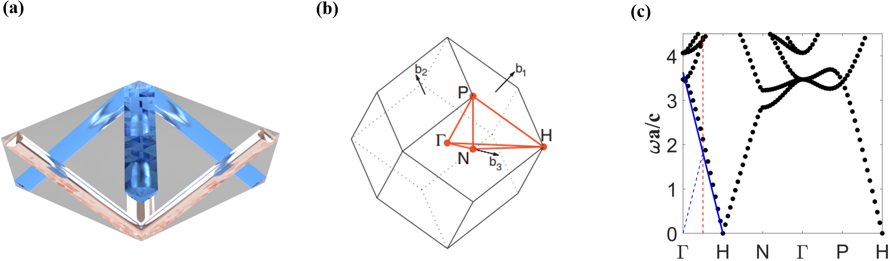
Here, we propose a generic hydrodynamic double fluid plasma (HDP) effective medium approach to generate new types of photonic BICs in double-net metamaterials (DNMs) consisting of two intertwining, spatially separated metallic networks [23, 24]. While the discussion in this paper is restricted to Cartesian wire meshes as shown Figure 1, we show that the HDP model equally applies to other DNM geometries in Appendix A (Figure A1 and Figure A2). In contrast to existing designs, the proposed BICs are formed by pure charge fluctuations of the electron acoustic wave (EAW)-like modes in DNMs, which are strikingly robust against a large class of perturbations. They exist within a broad spectral range free of non-BIC resonances and their frequency spacing can be freely tuned by the thickness of the structure, reaching spectrally dense BICs for an optically thick DNM slab. Additionally, new Zak-phase protected topological suface bound states in the continuum (TSBICs) are discovered in DNMs. Both bulk BICs and TSBICs exist at the -point of the in-plane Brillouin zone within the light-cone for DNM slabs, yet they are fully decoupled from radiation.
II Electronic acoustic wave in double-net metamaterials
The new types of BICs originate from a pure charge wave, which does not produce electromagnetic fields. Although impossible in conventional optical materials, this property can be found in non-Maxwellian materials [25], for example in an HDP. The hydrodynamic motion of two charge carriers in combination with Maxwell’s equations describes the fluid-like dynamics of an effective double plasma in an electromagnetic field. The full HDP model is derived in Appendix B. In short, we restrict the discussion to a non-dissipative model with only two free parameters: the plasma frequency and the thermal pressure parameter for the two charge carriers labelled . These depend on the equilibrium charge carrier density , the charges , the effective masses , the equilibrium pressure , the adiabatic exponent and the speed of light in vacuum .
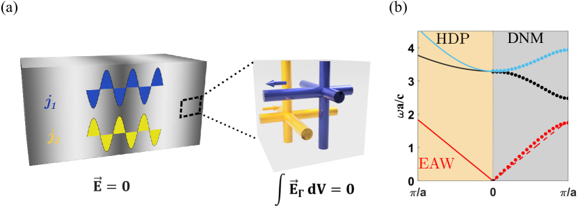
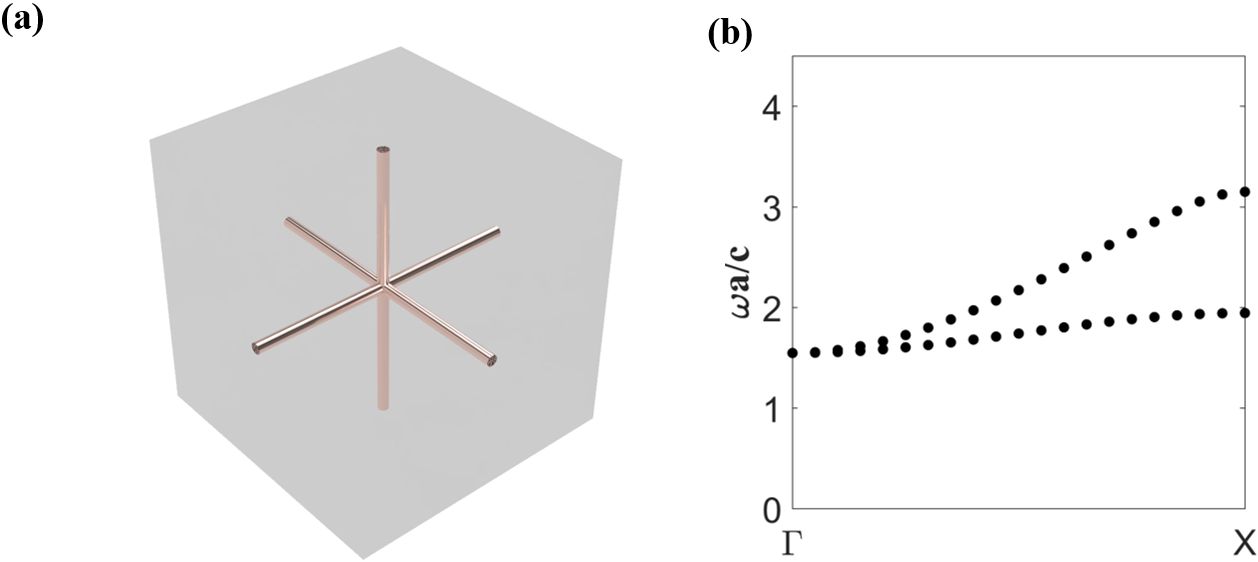
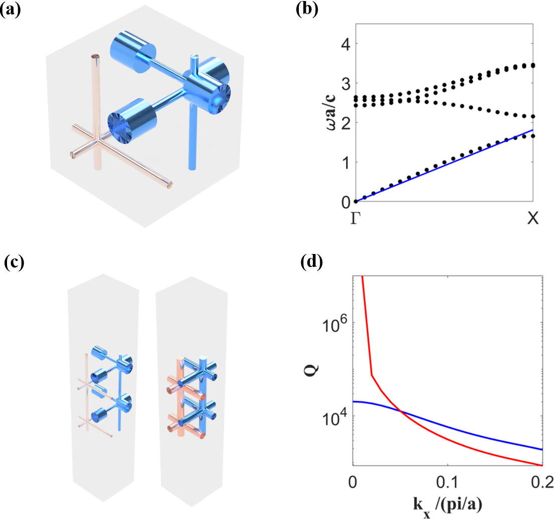
Through a plane-wave ansatz and by linearizing the HDP model [26, 27], the generally complex problem is transformed into a -dimensional linear eigenproblem for the eigenfrequency . As shown in Figure 1(b), from high to low frequencies, a two-fold degenerate electromagnetic transverse band and a longitudinal Langmuir band are obtained, both of which are hyperbolic starting at for wave number , and a linear electron acoustic wave (EAW) band emanating from . The slope of the EAW band is , as analytically shown by theory [28] (Appendix C). Regardless of , when , the EAW consists of two charge waves drifting in opposite direction, with current densities and vanishing electromagnetic fields (Figure 1(a)). Due to its zero electromagnetic nature and the resulting decoupling from the electromagnetic vacuum modes, the EAW naturally forms BICs.
To circumvent the difficulties in creating a natural double-plasma [29, 30, 31], we instead employ a finite DNM lattice, whose fully connected wire morphology effectively provides a freely moving double-plasma with finite equilibrium charge carrier density and Coulomb pressure, leading to a behavior that resembles a plasma with an exact electronic thermal pressure. Note that in DNMs, are largely determined by the connectivity of the wires, which leads to (Appendix B.2). The DNM structures discussed in this paper are composed of two single nets of fully connected metal cylinders along the cubic axes with radii , which may be different for the two nets. We use the notation to represent the network parameters, normalized by the lattice constant . is the offset of the two networks that are shifted by . Two parameter sets are discussed in this manuscript,

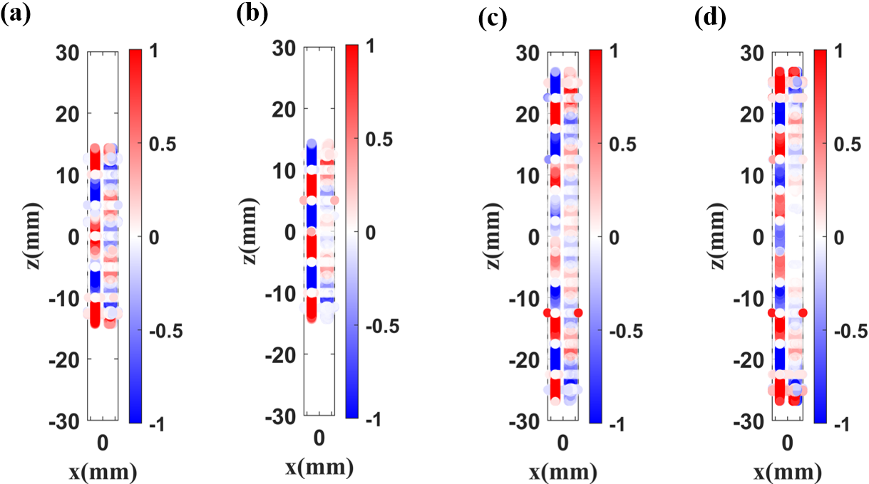
The numerically simulated band structure of the DNM is illustrated in Figure 1(b), featuring a linearly dispersed fundamental band (red dotted line) that emanates from the -point at zero frequency. This result not only qualitatively matches the EAW band in the HDP model, but the dispersion is indeed in good agreement with the analytical prediction from Appendix C (red dashed line). In the HDP model, the slope of the EAW band is largely independent of the plasma frequencies (Appendix B), which applies to a variety of DNM realizations (Appendix D), as confirmed by numerical simulations (Figure A6, A7). Analogously to the EAW in the HDP model, the two networks in the DNM carry opposing currents, indicated by arrows in Figure 1(a,b). Simulated surface current densities are shown in Figure 2(a,b) for DNMs with equivalent radii and different offsets ( and ). They indeed exhibit almost exactly opposite in the two networks at and . For different radii (, Figure 2(c)), a weaker current density is observed on the larger radius network, whose integrated magnitude equals the opposing current density of the lower-radius network. This implies that the total current remains zero, irrespective of the network radii, consistent with the HDP model.
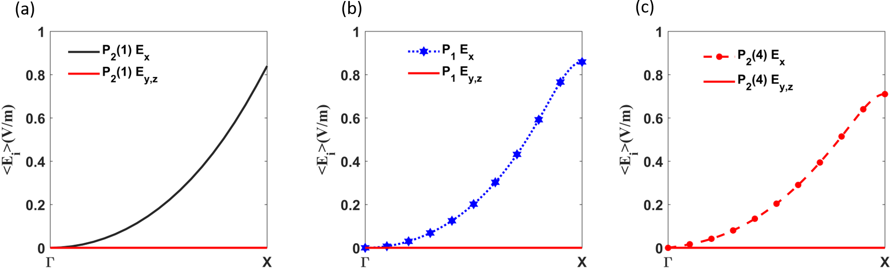
To investigate the nature of the microscopic electromagnetic fields of the EAW-like modes in DNMs, we compute the unit-cell-averaged electric field components of the fundamental mode, normalized by the averaged electric field intensity. The averaged transverse components vanish over the entire Brillouin zone (Figure A5), while the longitudinal component quadratically increases with the wave vector when moving away from (Figure 2(d)). The fundamental modes in DNMs are therefore quasi-longitudinal with . We conclude that the HDP model is a valid effective medium description for DNMs near the static limit and that DNMs provide a metamaterial realization of HDPs that require extremely stringent restrictions in natural plasmas, impeding their laboratory observation. We finally note that due to the non-Maxwellian nature of the EAW that lacks electromagnetic fields, the introduction of an effective permittivity seems misleading. In this context, for the network, a previously reported homogenization approach [32] leading to an effective permittivity for the DNM only accounts for the Langmuir mode residing at high frequencies. In contrast to standard metamaterial homogenization approaches, the HDP model developed here yields a fully consistent effective medium description of the fundamental DNM band and provides an accurate prediction of both the phase velocity and the associated fields.
III Bound states in the continuum in double net metamaterials
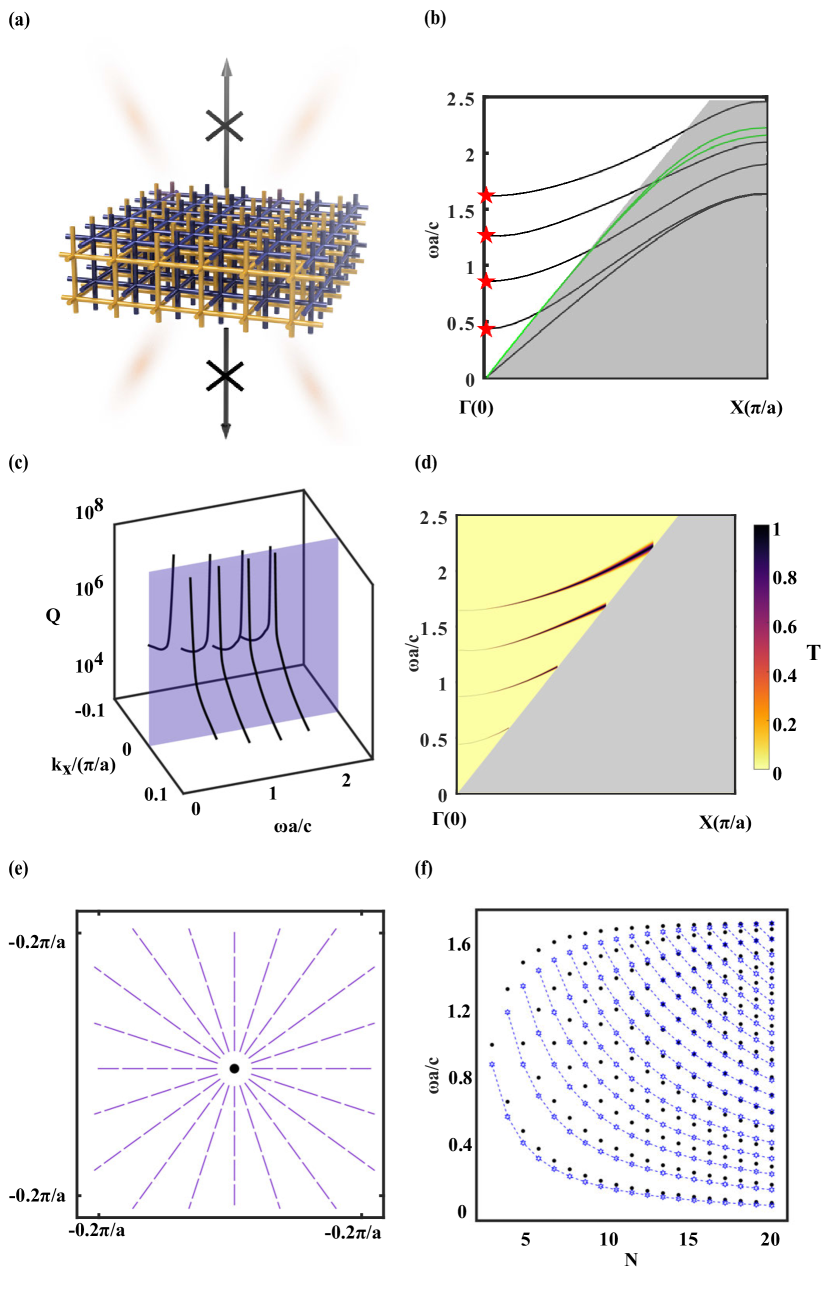
Here, we show that the EAW character of the bulk modes in DNMs naturally leads to the formation of a new type of BIC, if it is embedded in vacuum in a slab configuration, as illustrated in Figure 3(a). In the HDP picture, a standing wave solution exists at certain frequencies where the EAW solutions can be superposed so that the normal component of vanishes at the slab boundaries. As the EAW fields satisfy , they perfectly decouple from the radiative vacuum modes [33]. To illustrate the above prediction, we simulate a -layer slab of a DNM (Figure A18). We apply Bloch-periodic boundary conditions in the -plane and scattering boundary conditions in the -direction, and solve for the complex-valued frequencies. As predicted, multiple BICs with infinite lifetimes are found, located at the -point, marked by red pentagrams in Figure 3(b). The frequencies of the BICs are well approximated by the standing wave solution of the EAW with a predicted phase velocity of and hard wall boundary conditions (). The EAW band is well below the first Wood anomaly, so that the higher Bragg orders in the vacuum Rayleigh basis are evanescent and non-radiative [34, 35]. Because the EAW bulk band is spectrally isolated from the other non-evanescent bulk bands at low frequencies, the BICs are free of non-BIC slab modes in the entire spectral range of the EAW band. In contrast, BICs in photonic crystals are usually mixed with non-BIC modes [3].
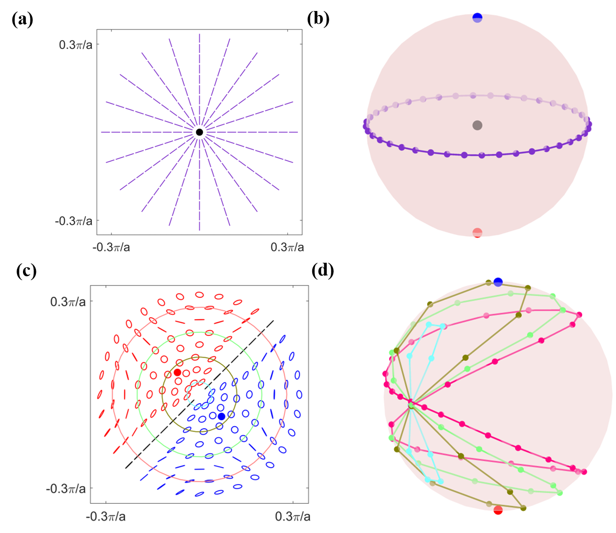
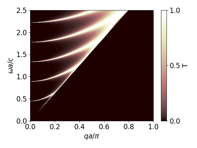
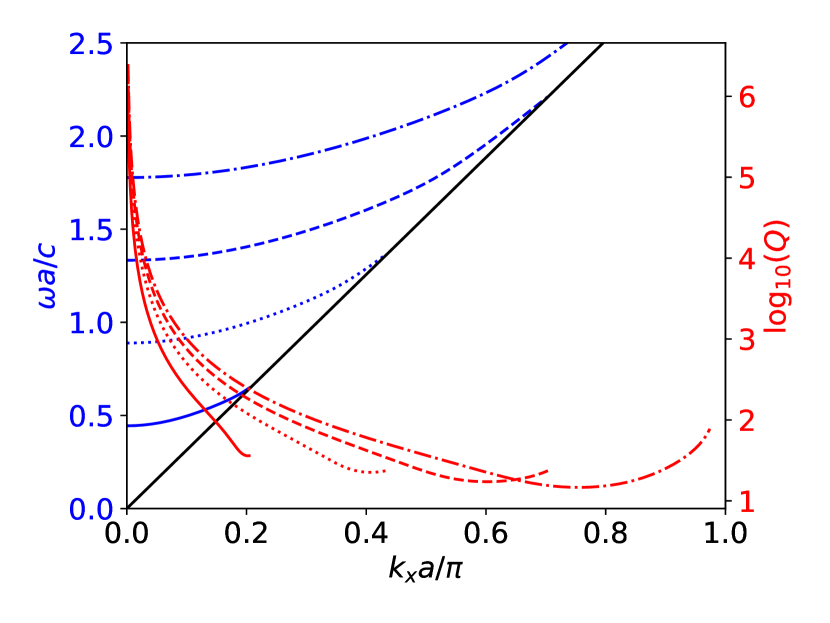
At finite wave vectors away from the -point, quasi-BICs are formed since the EAW fields are not strictly orthogonal to the vacuum plane waves, which results in a weak coupling to the vacuum states. These quasi-BICs thus have a very large, but finite, quality factor. The corresponding -factor values of the multiple quasi-BIC solutions in the vicinity of the -point are shown in Figure 3(c). The physics is reminiscent of a Fabry-Pérot resonator with mirrors that are perfectly reflecting at normal incidence and otherwise weakly transparent. In scattering experiments, this system yields a simple transmittance spectrum with a Lorentzian line shape at finite wave vectors close to the BIC frequency. The centre frequency forms a band that emanates from the BICs at the -point and hyperbolically blue-shifts with increasing wave vector, while the width of the Lorentzian gradually broadens. The simulated transmittance spectrum along the - direction is shown in Figure 3(d). The polarization of the quasi-BIC far-field is oriented in the direction of the wave vector, forming a ‘star’ pattern in 2D momentum space, as shown in Figure 3(e). At the -point where the BICs reside, this generates a singular point where the polarization cannot be defined since the far-field vanishes. Around this point, the polarization pattern evidently exhibits a non-trivial topological winding number [8]. In our case, this topological vortex structure of the polarization field is a direct consequence of the quasi-longitudinal nature of the EAW modes and is reminiscent of the electric field lines created by a point charge.
In photonic crystal slabs and metasurfaces, BICs are essentially symmetry protected and can be destroyed by infinitesimal symmetry-breaking perturbations [20, 21]. Strikingly, the new BICs formed in DNMs are immune to global symmetry breaking and are only prone to perturbations in the individual networks. The DNM slab with has indeed only one point symmetry, the mirror symmetry, which is insufficient to create symmetry-protected BICs in photonic crystal slabs that require at least two mirror planes. The stability of the DNM-based BICs can be attributed to the surface current densities on the metallic wires. For the EAW mode at , the currents on the two metallic cylinders along the -direction are exactly opposite (Figure 2(a–c)). and on each single net resemble electrical quadrupoles, whose form is determined exclusively by the the single net geometry, and which are found irrespective of the global symmetry (Appendix E, Figure A8). Since the interaction between the currents on the two nets is negligibly small in the static limit, the total radiated field from the quadrupole-like current vanishes, irrespective of their relative positions, radii, etc. This ultimately leads to BICs that are robust against global symmetry breaking. This robustness of the BIC modes is demonstrated in Appendix F through simulations of DNM slabs with various parameters (Figure A9). As shown in Appendix G, the BICs can, however, be lifted by breaking the local symmetry of individual nets (Figure A10), spawning circularly polarized points in the far-field (Figure A11).
Finally, since the BICs originate from the standing wave solutions of the EAWs in the DNM slabs, the number of BIC modes and their frequency spacing are exclusively determined by the thickness of the DNM slab. A full theoretical model that predicts both the quasi-BIC bands including their quality factors (Figure A13) and the transmission spectrum (Figure A12) is presented in Appendix H. In particular, the model yields BIC modes that are equidistantly spaced at frequencies of , where is the thickness of the DNM slab and . Extrapolating the linear dispersion relation of the HDP model to the Brillouin zone boundary, we expect BIC modes over the EAW band, which perfectly matches the full wave simulation results of the DNM in Figure 3(f). Generally, the theoretical results are in good agreement with the simulations even though the equidistant frequency spacing is of course perturbed in real DNMs.
IV Topological surface bound states in the continuum
Our theory builds on the HDP homogenization model that, while a powerful tool to understand the bulk modes and the formation of BICs, cannot capture the discrete periodicity of DNMs. This discrete lattice structure, however, bears additional features. For example, as predicted in [23], a primitive lattice translation of the network with BCC symmetry interchanges the two individual networks and results in an EAW band emanating from the corner of the Brillouin zone at the -point (), as shown in Figure A14 111When perturbed from , the symmetry is lowered to the simple cubic space group. The EAW band thus emanates from and it seems as if the mode discontinuously jumps from left-handed to right-handed propagation. The conundrum is resolved by realizing that the main Bragg amplitudes of the Bloch wave remain at non-zero reciprocal lattice vectors, causing a left-handed behavior that is not immediately evident from the bandstructure.. A lattice symmetry with an underlying highly symmetric isogonal point group can often be associated with non-trivial topological properties [37, 38, 39, 40]. As shown below, the lattice symmetry of the DNMs gives rise to a non-trivial Zak phase and topological surface bound states in the continuum (TSBICs). TSBICs exist at the interface between the DNM slab and vacuum within a radiation continuum, in contrast to typical topological surface states, which reside in bulk bandgaps of two neighbouring domains [41].
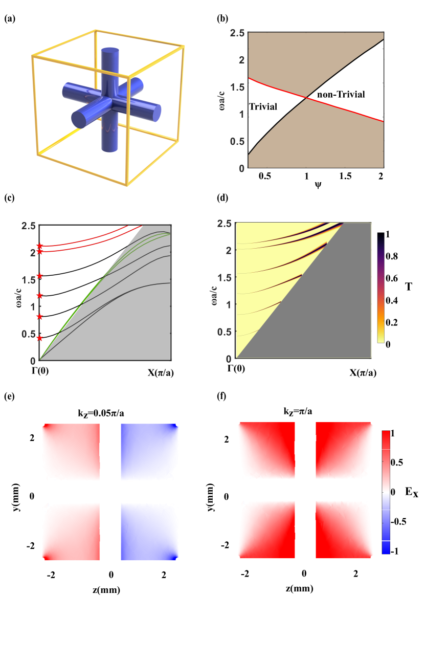
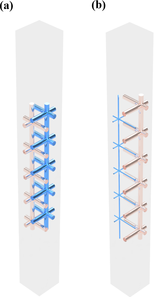
The emergence of TSBICs can be understood by examining the family of DNMs. A schematic diagram of a DNM is shown in Figure 4(a), with the corresponding bandstructure in Figure A15. For (i.e. equal network radii), the structure has the full body centered cubic (BCC) symmetry. As a result, the EAW and the Langmuir bands meet at , since they stem from one band that is back-folded half-way between the and the -point of the BCC Brillouin zone [42]. For , a bandgap opens as predicted by the geometrical perturbation theory described in [40]. In the presence of inversion and time reversal symmetry, the band topology can be characterized by a (binary) topological index, called the Zak phase [43], which is best known for the quantized bulk polarization of electrons in solids. The Zak phase is the well established Berry phase [44] evaluated across a 1D Brillouin zone, which is topologically a circle and therefore closed. It is generally a continuous number on that depends on the choice of the unit cell. The Zak phase is, however, -quantized, with values of and , if the unit cell has a parity symmetry in its center [45]. Therefore, an offset of between the two nets is necessary to preserve the Cartesian mirror planes in the point symmetry of , allowing a Zak phase classification.
In our case, the Zak phase is obtained by examining parity of the electromagnetic Bloch fields at the high symmetry points of the 1D Brillouin zone [46]. We make use of the mirror plane (operator ) in the centre of unit cell in Figure 4(a). The fields must have even () or odd () parity with regard to at the and -points, where the wave vector is invariant under . The Zak phase of the band has been shown to be the complex argument of the product of both parities [46]. A topological phase transition from trivial to non-trivial Zak states is observed in the projected band structure shown in Figure 4(b) at , where the network has the higher BCC symmetry and the bandgap closes at the -point of the simple cubic Brillouin zone. The field parities for are illustrated by the -components of the periodic part of the electric Bloch field of the EAW mode close to 222On itself, the numerical full wave solution yields a multi-dimensional eigenspace, including spurious modes, with no simple 1D even/odd representation of the mirror group. in Figure 4(e) and at in Figure 4(f). For a DNM slab terminated at its thin wires, we therefore predict, and indeed see, topological surface states within the bandgap, shown as red lines in Figure 4(c). Note that the DNM slab is truncated slightly away from the mirror plane through the thin wires as shown in Figure A18(b), to avoid slicing the thin wire. As discussed in Appendix J, an energy difference between the two surface states is observed, which is caused by hybridization of the surface states on either side of the slab through its finite thickness (Figure A16). The interaction is weakened by increasing the slab thickness, as shown in Figure A15(b).
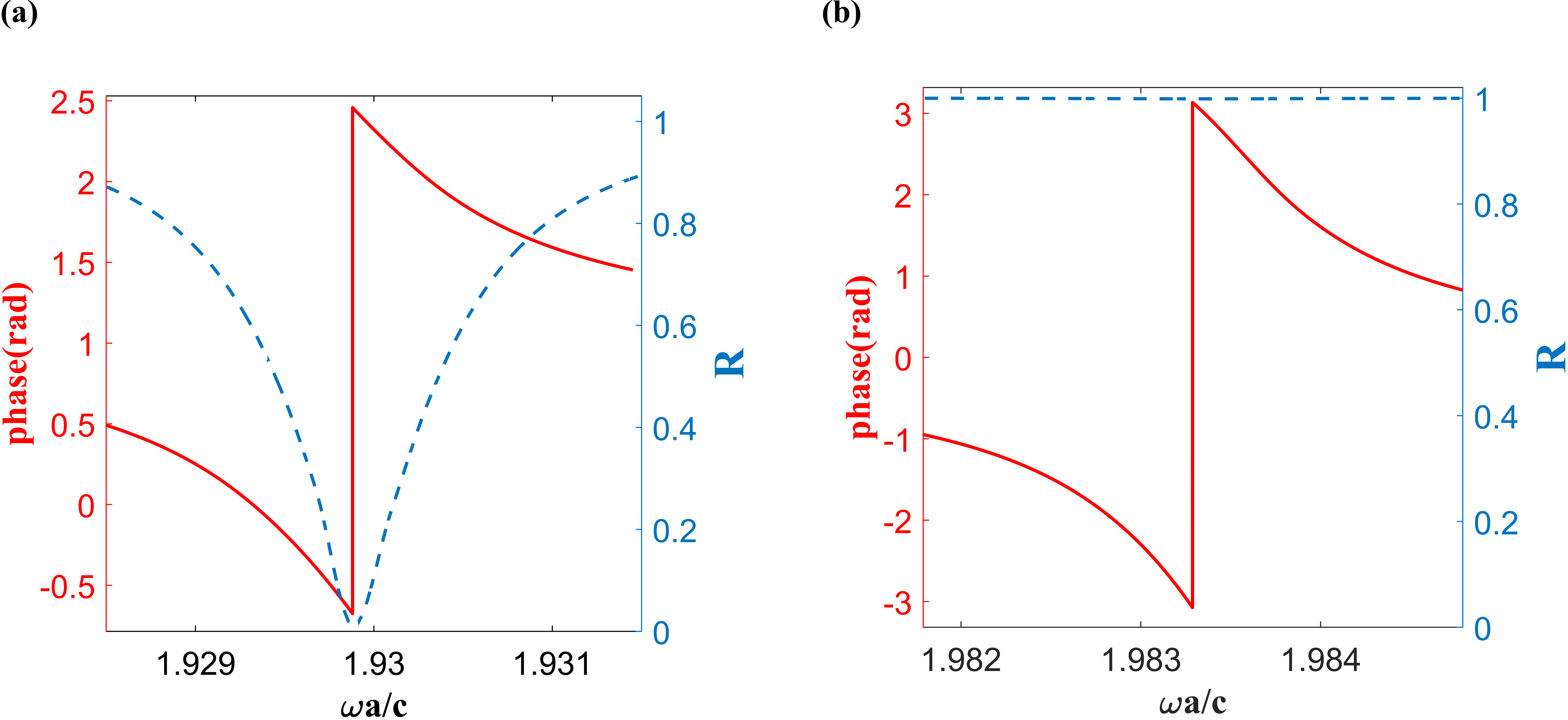
The topological surface bands in Figure 4(c) are evidently associated with high -factor quasi-TSBIC bands revealed by the reflectivity plot in Figure 4(d). TSBICs are, in stark contrast to conventional photonic topological surface states [41], confined through the EAW mechanism and do not require a surrounding topologically trivial band-gap material. When different terminations are applied to the top and bottom surfaces, so that only one surface obtains TSBICs, no resonance is found in the reflection/transmission amplitudes, since no hybridization, which provides a direct transmission channel, occurs. The presence of a single quasi-TSBIC band manifests itself, however, in a resonance in the reflection phase (Figure A17). Despite earlier reports of surface BICs in terms of the intrinsic continuum in the material [6], our TSBICs constitute the first example of BICs of topological origin which are decoupled from free space radiation. Controlling the coupling between the topological surface states with free space light could pave the way towards both fundamental scattering properties of topological states and their application, for example in topological antenna arrays [48].
V Conclusions
We have demonstrated a new deterministic route towards photonic bound states in the continuum in double-net metamaterials. A hydrodynamic double fluid plasma serves as an effective medium model for these materials. The hydrodynamic double plasma yields an analytical solution with a new type of quasi-longitudinal EAW band, which gives rise to photonic bound states in the continuum that are robust even against strong geometrical perturbations and symmetry breakings.
Moreover, topological phase transitions are found in double-net metamaterials, accompanied by topological surface bound states in the continuum, protected by a Zak phase topological index. The marriage between the bound-state behavior and the non-trivial topological phase enables the lossless existence of TSBICs even for open boundaries. Our findings endow using double-net metamaterials as a new platform for the realization of photonic bound states in the continuum by employing a new topological strategy. Advances in 3D fabrication, particularly the 3D printing of metals, enables the manufacture of the proposed double-net metamaterials. While an experimental verification of our predictions is thus readily available at microwave frequencies, we intend to extend our findings to higher frequencies, allowing to, for example, facilitate quantum emission from the coherent spontaneous emission regime, over photonic Bose-Einstein condensation to lasing applications.
Acknowledgements.
We would like to thank Ullrich Steiner for fruitful discussions and general support. We acknowledge funding by the Swiss National Science Foundation through the Spark Grant 190467 and the Project Grant 188647.Appendix A Different double network geometries
While our theory above has been rigorously derived for the pcu double network only, the two main physical features are inherent to the plasmonic double network topology and symmetry rather than the particular geometrical realization. These features are the slope of the EAW band in the low frequency limit and the longitudinal nature of the homogenized electric field. We here demonstrate that both features are indeed be observed for two other established double net geometries: the balanced double gyroid (srs-c, symmetry) and double diamond (dia-c, symmetry) morphologies (abbreviations as in [49]).
Let us first re-examine the longitudinal nature from a symmetry perspective. In the quasi-static limit, a non-trivial solution to the Poisson equation requires the two nets to be on different potentials [23]. Three situations can generally be distinguished:
-
1.
the two nets are only interchanged by one or more space group elements with point symmetry part that is not the identity333In other words, we have in Seitz notation with a point symmetry and a translation part , which might be non-zero (screw axis or glide mirror for example).,
-
2.
the two nets are interchanged by a primitive lattice translation444 in Seitz notation, where must be a primitive lattice vector.,
-
3.
the two nets are no symmetry copy of one another. This case is always possible for unbalanced double nets as for example the qtz-qzd double net [52].
The cubic examples discussed here all belong to the symmetric cases 3 and 4. In these cases, the square of the symmetry operation that exchanges nets evidently maps the two nets onto themselves. The potential is therefore unchanged by as the individual nets are short-cut in the quasi-static limit. As a consequence, yields a multiplication of the potential by and the two nets must hence be on opposite potential. In case 3, the Bloch character is trivial and the EAW band emanates at zero frequency at the -point. In case 4, the Bloch character is with respect to a primitive lattice translation and the EAW hence emanates at zero frequency at the corner of the Brillouin zone.
With these preliminary considerations in mind, we first revisit the pcu-c double net. As the pcu-c evidently belongs to case 4 above, with a primitive body-centered cubic lattice translation interchanging nets, the EAW band emanates at zero frequency at the point [42]. Since lies along the cubic direction, any state at the center of the surface Brillouin zone (with vanishing lateral ) of a inclinated slab is therefore made by a superposition of counter-propagating EAW modes along -. The behavior in the quasi-static limit now further yields the irreducible representation, or irrep, of the electric field with respect to the group of the wave vector [28], which is the point group in this case. Since all elements of do not interchange networks and the individual networks are on constant potential in the quasi-static limit, the EAW irrep is trivial. Therefore, the homogenized field cannot have a component perpendicular to the wave vector direction, as these would transform with a non-trivial 2D irrep. The fields must be longitudinal from a symmetry perspective over the whole EAW and Langmuir bands, which are glued together and form one band.
The srs-c is of case 3 above, and the EAW band emanates at the -point of the body-centered cubic Brillouin zone at zero frequency. The bandstructure along ( with ) for wire radius of is shown in Figure A1 (a). It agrees perfectly with the HDP prediction for the corrected pressure parameter of for the wire radius of over the whole band. This can be understood as follows: The group of the wave vector is again , which is isomorphic to the abstract group in [53]. Considering the quasi-static potentials, the EAW band must be even with respect to the screw rotation and the rotation (which map each single net onto itself), and odd with respect to the glide mirror planes (which interchange networks). It therefore has the 1D representation in . At the point, the EAW joins a -fold degenerate point, which transforms according to the representation in , which splits equally into the 1D and one 2D representations along -: . This allows the representation to form a pair with its time reversal symmetric representation to form a back-folding at with finite and opposite slope of the two bands.
As in the pcu-c scenario, the longitudinal EAW behavior is protected by symmetry. Since the group of the wave vector contains a screw axis and diagonal glide mirrors that both contain a shift along the propagation direction, only the non-symmorphic wallpaper subgroup (number in [54]), with isogonal point group, can be employed to make a general prediction regarding the homogenized fields. Considering the quasi-static potentials again, we obtain an even symmetry classification with respect to the symmetry in . This classification evidently does not permit homogeneous field components perpendicular to the direction of the wave vector. The odd symmetry behavior with respect to the glide mirror symmetry in on the other hand prohibits a homogenized field component along . For the srs-c, we therefore expect a truly vanishing homogenized electric field that extends over the whole EAW band. This vanishing field is demonstrated in Figure A1 (b) within the numerical precision of the simulations (note the logarithmic -axis).
Similar to the pcu-c, the dia-c network with simple cubic symmetry belongs to case 4 above. The EAW band therefore emanates at the simple cubic -point [42]. Consequently, the EAW band lies outside of the light cone along the cubic and directions and cannot lead to BICs. For a slab with inclination, however, the EAW band along the path connecting with ( with ) lies at the center of the surface Brillouin zone. The low frequency dispersion agrees again perfectly with the HDP prediction with corrected as shown in Figure A2 (a). It therefore yields BICs by the same mechanism as exploited in the pcu-c case with slab inclination of , assuming a longitudinal homogenized electric field. Such a field is guaranteed by the trivial symmetry classification of the mode with respect to the group of the wave vector555Even though is non-symmoprhic, the elements of the group of the wave vector (labelled 1, 5, 9, 38, 43 and 48 in [54]) are pure mirrors and rotations through the crystallographic origin., which only allows a homogenized field parallel to . This longitudinal nature is once again demonstrated through full wave simulations in Figure A2 (b).
Appendix B Plasma and pcu network modes
B.1 Single plasma fluid model
We begin with a single plasma fluid model for a warm plasma [56]. This model consists of a set of three equations describing the charge carrier (CC) dynamics,
| (1a) | ||||
| (1b) | ||||
| (1c) | ||||
Eq. (1a) is the continuity equation of CC conservation, where is the CC volume density field and is the CC velocity field. Eq. (1b) is the Navier-Stokes equation for the electrically excited CC liquid, where we ignore shear forces, the non-linear magnetic field contribution in the Lorentz force density, and gravitational contributions. In this equation, is the outer product, the effective mass of the charge carriers, the CC liquid pressure field, and the CC charge density. We note that a kinetic pressure term is present in any liquid. Here, should be understood as the total mesoscopic pressure based on the microscopic statistical ensemble of CCs, including inter-particle Coulomb interactions. Finally, Eq. (1c) is a local adiabatic equation with the adiabatic index , which can be rigorously derived from an energy balance equation in the limit where the flow velocity is much larger than vicious and thermal diffusion velocities [56]. These fluid equations are closed with the Maxwell curl equations, which describe the electro-magnetic field dynamics. In Lorentz-Heaviside units,
| (2a) | ||||
| (2b) | ||||
with and the electric and magnetic fields, respectively, the speed of light in vacuum, and the current density of the plasma charge carriers.
We now linearize Eq. (1) assuming small variations in the density and pressure
and thus small velocities to arrive at
| (3a) | ||||
| (3b) | ||||
| (3c) | ||||
Since if , Eq. (3c) is solved by . Finally, since Eq. (2) and Eq. (3) are now both spatio-temporally homogeneous and linear in all fields, we can make a plane-wave ansatz , etc., such that the field symbols represent their constant coefficients from this point on, to obtain
| (4a) | ||||
| (4b) | ||||
| (4c) | ||||
| (4d) | ||||
We now introduce the plasma frequency , the plasma wave number , and the dimensionless pressure parameter , to obtain a -family of linear Hermitian eigenproblems
| (5) |
for the eigenvalue . The eigenvector is defined as
The dimensionless matrix operator
| (6) |
which we from now on refer to as Hamiltonian, has the sub-blocks
| and |
Here, we have used the Pauli spin matrix , the vector product matrix , the Kronecker (tensor) product , the zero vector and matrix of dimension , and the identity matrix of dimension ; denotes the Hermitian adjoint of .
The problem is of course isotropic, so that we can choose the coordinate frame such that without loss of generality. The eigenproblem Eq. (5) predicts a four-fold degenerate zero-frequency band . The associated eigenspace is spanned by two longitudinal spurious modes, which violate the Maxwell divergence equations, and the static magnetic field solutions generated by a transverse current density
at constant charge and vanishing electric field.
Note that the system is particle-hole symmetric [57], that is, for every eigenvector of with energy , there is one particle-hole symmetric eigenvector with energy . Thus we just show the positive frequency bands in Figure A3. They follow the longitudinal mode Langmuir dispersion666Note that we do not normalize fields and choose the electric and magnetic field without dimension (instead of their standard cgs unit ) here for convenience.
| (7) |
with fields , , , and ; and the two-fold degenerate transverse light mode dispersion
| (8) |
with fields , , , and .
B.2 The metal pcu wire-mesh
At low frequencies in the microwave regime, most metals act like prefect electrical conductors (PECs), which do not support propagating modes in the bulk. Employing plasmonic metal wires, we can however reduce the CC density to introduce an effective plasma freqeuncy for excitations in the wire direction, while maintaining the lossless PEC character [59]. A 3D metallic pcu [49] wire-mesh with sub-wavelength period therefore effectively generates a lossless plasma at microwave excitations. Based on [60], we here formally show that the electro-dynamic theory of the metallic pcu network in the long wavelength limit, is indeed equivalent to the single plasma model with a constant pressure parameter .
We use the macroscopic constitutive relations from [60] that have been derived for a square lattice of aligned wires (along ) in the homogenization picture. We start with the current and the electric potential between neighbouring wires. A comparison of the magnetic flux through a rectangle of infinitesimal height with the corresponding boundary integral (Ampére’s law in integral form) yields (assuming a plane-wave form)777Note that we here use the physics convention for the monochromatic ansatz and Lorentz-Heaviside units in contrast to [60].
| (9) |
with the self-inductance per unit length of the wires in the mesh that is a simple consequence of the Biot-Savart law for the individual wires and only depends on the lattice constant (nearest neighbour distance) and the wire radius . The potential between neighbouring wires is on the other hand related to the linear charge density via the linear relation with the effective capacitance per unit length that is obtained using Gauss’ law. Combining this relation with charge conservation leads to
| (10) |
Eq. (9) and Eq. (10) can be readily generalized to a 3D connected pcu wire-mesh: Eq. (9) simply acquires full vector form with , , and . The linear charge density is effectively reduced by a factor of as the charges spread over three wires in each direction in the unit cell and the pcu network is fully connected. A more rigorous treatment for wires of finite radius reveals that this factor is indeed better approximated by [62]
| (11a) | ||||
| with the plasma wavenumber | ||||
| (11b) | ||||
| (11c) | ||||
In practice, the wire-mesh pressure parameter falls in a range between for a wire radius of and for . Rearranging, we obtain
| (12a) | ||||
| (12b) | ||||
Defining the plasma frequency as the cut-off frequency of the aligned wire mesh [59] , which is indeed a good approximation of the definition in Eq. (11b), and the field vector
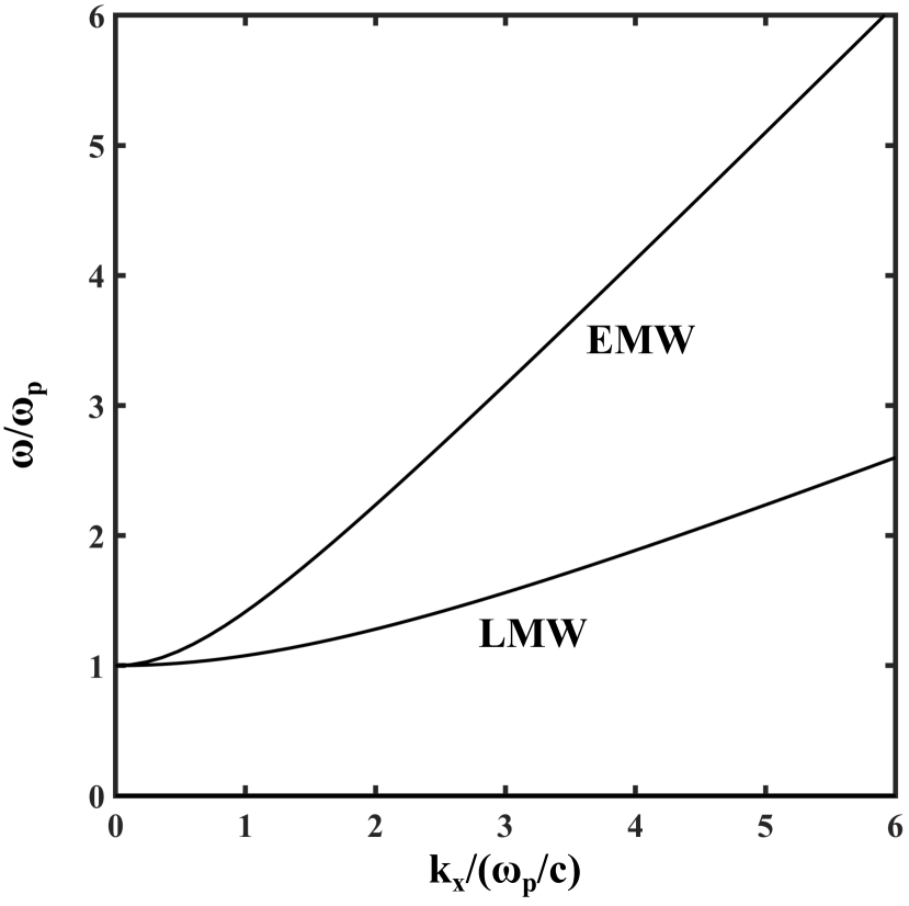
we formally arrive at the above eigenproblem Eq. (5) with a that is confined in a small interval and only weakly depends on the geometrical parameters of the wire-mesh. We finally note that the scaled potential equals the scaled CC density fom Section B.1, if we associate the linear charge density along the PEC wires per unit cell area with the charge density of the plasma, so that the field vector is identical in both models. Figure A4 shows the bandstructure obtained through a full-wave simulation, which agrees well with the single plasma fluid model shown in Figure A3. The two modes in Figure A4(b) correspond to the longitudinal (LMW) and transverse (EMW) modes in Figure A3.
B.3 Hydrodynamical double plasma fluid model and plasmonic double pcu wire-mesh
We now consider a plasma consisting of two CC species of respective charge , mass , and equilibrium CC density and pressure (). The associated plasma frequencies, plasma wave numbers and pressure parameters are, and . We further assume that CC interact only amongst their own species, which is physically of course only possible in a universe where particles of a different type do not interact (via Coulomb forces or otherwise). The theory is, however, approximately valid if the interaction is weak or if the two charge carriers are separated on a mesoscopic scale.
In the prescribed situation, the corresponding fluid equations Eq. (4c) and Eq. (4d) separate into two individual equations, while both current densities contribute to the Ampère-Maxwell law Eq. (4b),
| (13a) | ||||
| (13b) | ||||
| (13c) | ||||
| (13d) | ||||
As we have shown in Section B.2, a PEC pcu wire-mesh acts like a single plasma in the homogenization regime, that is if the Bloch wavevector of the mode satisfies . We use the parameter vector to define a pcu double network, where are the individual network radii and the lattice constant, and is the offset in each Cartesian direction, so that the two networks are separated by a shift vector . Assuming that the networks are well separated, the DNM fields therefore obey Eq. (13) with the substitutions discussed in Section B.2.
The two networks generally exhibit different plasma frequencies that depend on and lie approximately between for and for . The pressure parameters are generally also different, but contained in a very small intervall between and , so that it is useful to introduce and with . The canonical field vector of the double wire-mesh is therefore
The eigenproblem can be written as
| (14) |
with the associated Hamiltonian
| (15) |
with the sub-blocks
and
With w.l.o.g. because of the isotropy of the problem, this double-net eigenproblem yields the longitudinal band
| (16) |
with fields ; and the two-fold degenerate transverse light band
| (17) |
with . Similar to Section B.1, the zero-frequency band is -fold degenerate, with two spuriouos longitudinal solutions and now four transverse current modes with
| (18) |
and all other fields vanishing.
Importantly, a new fundamental band appears below the plasma frequency. It emanates at the -point at with constant slope as shown in the main manuscript in Figure 1(b). The associated modes are reminiscent of acoustic waves in a conventional fluid, but with two species of charges fluctuating in opposite directions. The dispersion relation is
| (19) |
with fields (in leading order in ) , , and . As we can see, the magnetic field of the EAW is strictly zero, while the electric field is longitudinal and linearly depends on both and . In the real DNM structures, since the HDP model is only approximately valid, the electric field of the low frequency mode obtains and additional longitudinal term that is zero order in and quadratic in . We demonstrate this behavior in Figure A5 by averaging the fields obtained through full wave simulations for three different DNM geometries. In Figure A5 (a) and (b), the -component increases quadratically when moving away from the -point, while the and components vanish for all . In Figure A5 (c), there is an additional small linear dependence as . In any case, the EAW modes in DNMs are evidently quasi-longitudinal.
Appendix C Effective Hamiltonian
The solution of the eigenproblem of the HDP associated with the Hamiltonian in Eq. (14) can be obtained algebraically using any standard computer algebra tool. A manual solution can, however, be more conveniently and elegantly obtained through the application of perturbation theory at the -point. Note that this procedure is exact when applied to the EAW band, as we shall see below.
Let us briefly summarize the general approach [28]. We first expand the eigenstates at some (at the -point we have ) in reciprocal space on the basis of those at , where has infinitesimal length. Consider the solution of the Hamiltonian at to be known for the eigenspace belonging to some eigenvalue . We thus define the orthonormalized eigenvectors that span , such that
If the components of the Hamiltonian are analytical at , we obtain in first order in ,
At the perturbed point , the eigenvectors are an element of in zero order perturbation theory. This immediately yields the identity (using Einstein notation),
As a result, the eigenvalue equation at becomes
Upon testing with , we obtain its weak form, which is an algebraic eigenvalue equation that has the dimension of ,
| (20) |
In other words, the deviation of the eigenvalues from is given by the eigenvalues of the effective Hamiltonian , whose entries are the matrix elements of the first order perturbation in . Since is linear in for the HDP Hamiltonian Eq. (15), the first order expansion is exact, that is with
Since we are interested in the eigenspace of at vanishing frequency, we are searching for its kernel, which is -dimensional and contains arbitrary , arbitrary or , and arbitrary , with all other fields vanishing. Labelling the field components in with and disregarding the trivial electrostatic solution with , we thus obtain the -dimensional eigenspace matrix with orthogonormalized eigenvectors as rows
The effective Hamiltonian is thus
| (21) |
where
Three of the eigenvalues of the perturbation Hamiltonian in Eq. (21) are zero. In addition we reproduce the EAW band in Eq. (19) and its chirally symmetry counterpart:
Evidently, the EAW slope only weakly depends on the difference in plasma frequencies of the two networks in first order . Particularly, if the two networks have equal radius, the slope of the EAW band is fully determined by the pressure parameter only. Generally, we note that the dispersion of EAW band in the low frequency limit is robust against changes in the DNM parameters such as the radius of the metal wires and the relative offset between the two nets. This assumption is verified by simulating DNMs with various parameters, shown in Figure A6 and discussed in Section C.
Appendix D Bandstructure of DNMs with different parameters
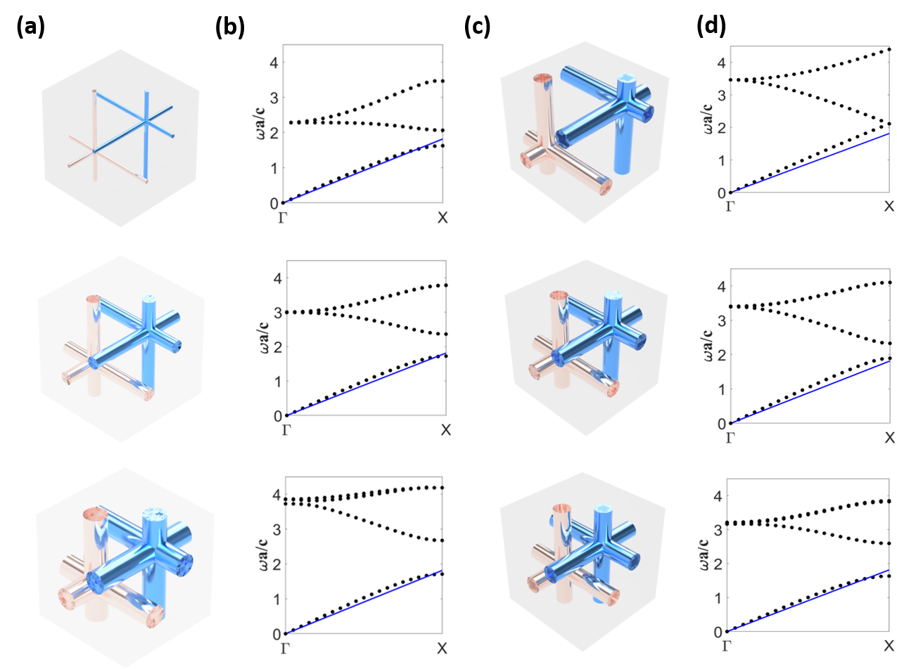
In Section B, we homogenized the DNM with an HDP model. We established that the EAW mode in the DNM is equivalent to two species of charged particles moving in opposite directions. From this model, we further obtained an exact dispersion relation Eq. (19) in the long wavelength limit, which mainly depends on the average pressure parameter of the two networks, which is . To verify this statement, we numerically simulate DNMs with different radii (Figure A6(a)-(b)) and relative positions (in Figure A6(c)-(d)).
In Figure A6(a) we begin with two wire meshes with a fixed relative space offset and different plasma frequency tuned by the (equal) radius of the two wire meshes from , over , to . The corresponding bandstructures are shown in Figure A6(b). The black dots are from full wave simulations, while the blue solid lines show the limiting dispersion. As expected, the DNM slope in the vicinity of the -point is larger in all three cases, and approaches the limit for small radii. The model is of course invalid when approaching the -point, due to the intrinsic non-homogeneous and periodic nature of the DNM structures. In Figure A6(c), we demonstrate DNMs with various offset while keeping the plasma frequency of both nets equal and constant (the radius is ). The bandstructures are shown in Figure A6(d). The results are again consistent with the theoretical expectation from the HDP model. Upon close inspection, the low frequency slope approaches the blue limit, when the two networks come closer together.
To further verify the validity of the HDP model applied to DNMs, we demonstrate an extreme case In Figure A7 with a huge difference in radius of the two nets.
Appendix E Quadrupole-like currents in DNMs with different parameters
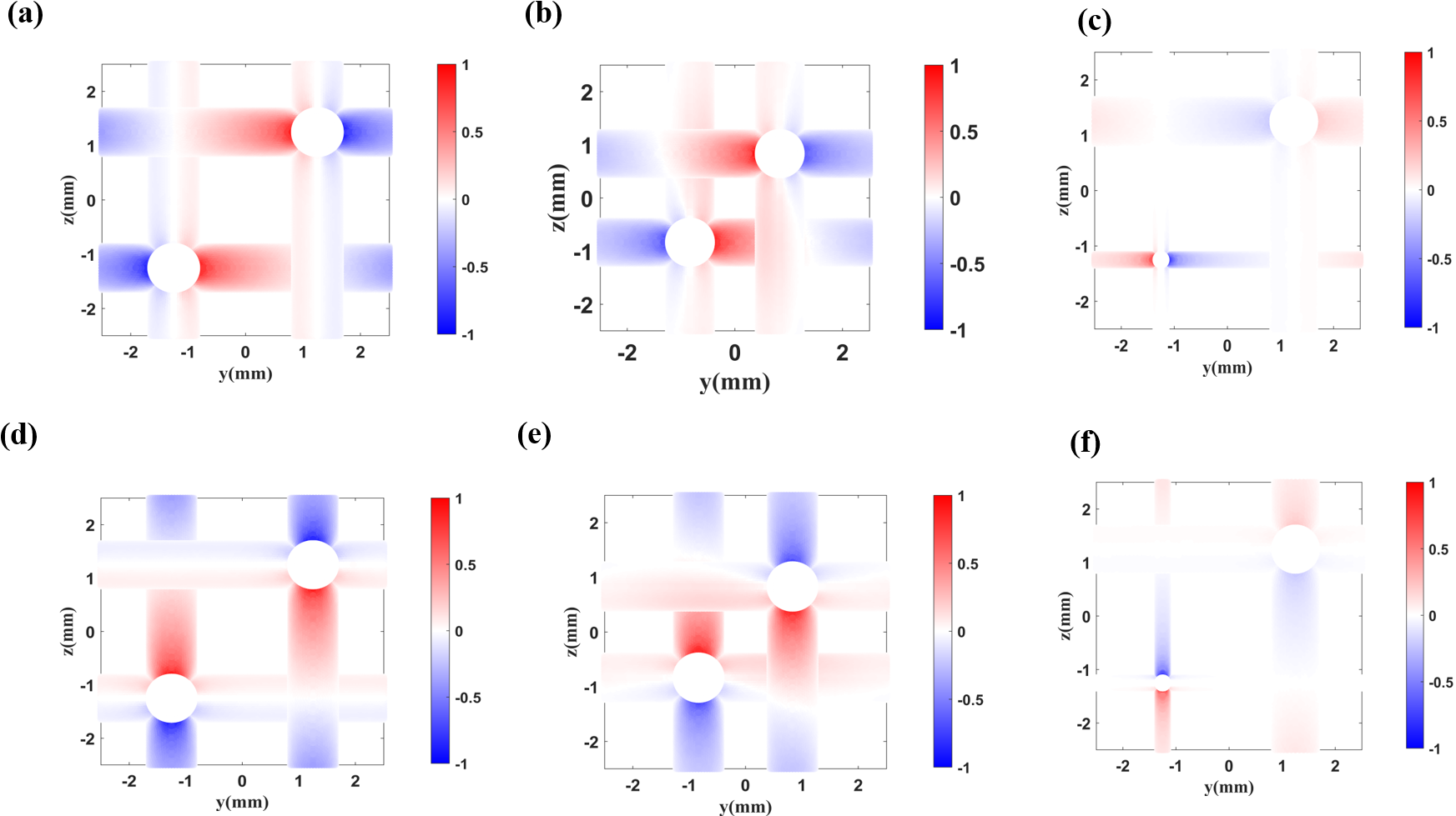
The surface current densities of the two nets in DNMs parallel to the propagation direction, with opposite signs, resulting in a vanishing homogenized electromagnetic field when approaching the -point, as shown in Fig. 2 in the main text. Meanwhile, small currents flow in the wires oriented perpendicularly to the propagation direction, which we refer to as w.l.o.g., at finite frequencies. The pcu-c DNM with body centered cubic symmetry has a global symmetry through the center of each of the wires. Since the currents in the wires are constant along the wire surface, they transform trivially under the corresponding symmetry. As a consequence, the weak EAW currents in the wires in the - plane must transform trivially as well, and therefore either all flow towards the nodes or away from them in a -fold quadrupole-like fashion. This expected behavior is demonstrated through the surface current densities obtained from full wave simulations, whose component is shown in Figure A8 (a) and the component in Figure A8 (d).
Notably, the in-plane geometry of the individual nets dominates the electromagnetic distribution, since the currents on the two nets experience very weak inter-coupling at low frequencies. The local symmetry of each single net thus guarantees the formation of the aforementioned quadrupole-like current distributions, even in the absence of a global symmetry. We demonstrate this behavior through the current distributions shown in Figure A8(b) and (e) for DNMs with a non-symmetric shift, and in Figure A8(c) and (f) for distinct wire radii. To a very good approximation, these fields retain their trivial character with respect to the individual net’s symmetry. Importantly, this trivial character is evidently incompatible with the free space photon modes, which carry the non-trivial character of the (right and left circular polarization) irreducible representation [63].
Appendix F BICs in the DNM immune to global symmetry breaking
The in-plane cross-shaped geometry which intersects perpendicularly by identical metal pillar of each individual wire mesh keeps the symmetry. The cross-shaped metallic pillar guide the surface density current, forming two quadruples in the space. The coupling between the two electrical quadruples is weak which is also the mechanism causing the BICs modes in DNM slab to be immune to the global symmetry. In the main text, we show the DNM slab with the parameters R(0.4,0.4) and offset (a/3, a/3,a/3). To further illustrate robustness of BICs in DNM, we show numerical results of DNM slabs with various parameters in Figure A9, all of which host BIC states.
Appendix G Lifting BICs by breaking local symmetry
Throughout this work, we have considered the metals constituting the DNMs as perfect electric conductors, so that surface currents flow on the metallic wires and determine the microscopic electromagnetic modes. We have shown in Section F that the surface current density forms two quadrupole-like distributions, which are robust against global symmetry breaking. These quadrupole currents are in the 1D representation of the point group labelled in [28], and thus cannot couple to vacuum radiation, which is in the 2D representation. However, the BICs can be destroyed by breaking the local symmetry of the individual nets in the DNM. We demonstrate this by introducing an thick metal cylinder segment on the lateral wires along the and directions normal to the slab direction (Figure A10(a)). These additional cylinders are arranged in such a way that the symmetry is reduced to a single mirror plane on the diagonal. For simplicity, we leave the other net unperturbed. The broken local symmetry, reduced to merely a mirror group, enables couplings of the EAW mode to vacuum modes. When compared to the DNM with two identical unperturbed wire meshes, the slab formed by the perturbed DNM (Figure A10(c)) degrades the BIC modes at the -point to quasi-BICs with finite -factors (Figure A10(d)). It is, however, worth noting that the perturbed DNM slab can still be well described by the HDP theory, as illustrated by the bulk bandstructure along the out-of-plane direction in Figure A10(b), which retains the typical EAW band.
The nature of the quasi-BICs, on the other hand, necessarily imposes changes in polarization structure in the far field. Compared with the ‘star’ polarization pattern of the BICs in the unperturbed structure (Figure A11(a)), the perturbed DNM slab exhibits a richer polarization distribution, forming two patches of elliptically polarized states with opposite handedness, separated by a diagonal linear polarization line (Figure A11(c)). The position of this line on the diagonal is evident from the fact that the in-plane components of both the dominating longitudinal currents and the quadrupole currents are even with respect to the remaining mirror if the mirror coincides with the plane of incidence, that is, if the wave vector is invariant. Thus, the far-field must obey the same symmetry classification, that is, it must be polarised, with the electric field confined to the plane of incidence. In all other directions, the EAW field is a combination of even (quadrupole currents) and odd (in-plane longitudinal currents) contributions, and thus the far-field is generally elliptically polarized.
The mirror plane divides the plane into two half-planes of opposite elliptical polarizations, which is immediately evident from the action of mirror symmetry on the modes on one half-plane. The vortex at the origin splits into two circular polarization points on either side. This mechanism is similar to the one reported in [20]; it is of topological origin. The appearance of the circular polarization points becomes evident from tracing the polarization on various momentum space circles of different raddi centered around the -point (Figure A11(c)). The polarization path projected on the Poincaré sphere goes twice through the linear polarization state on the mirror plane and unfolds from a small figure-of-eight (turquoise, small radius) towards a double-loop around the equator (grey, large radius), and thus necessarily passes through the north/south poles (Figure A11(d)).
Figure A11 further indicates that the circular polarized points lie on the axis perpendicular to the remaining mirror plane. We can understand this behavior from a symmetry perspective. Consider the action of the time-reversal operator , which transforms the slab mode with wave vector into one with and complex conjugated field, that is . The mirror symmetry on the other hand interchanges the and components of the field and also maps to its negative. The combined operation thus leaves invariant on the line perpendicular to the mirror plane. We thus obtain , so that the normalized in-plane electric far-field depends on one free parameter only,
In other words, the field stays on a line of constant longitude on the Poincaré sphere, connecting zero linear polarization along the mirror plane (at ) and perpendicular to it (away from for small perturbations). It must therefore pass the circular polarized poles () on either side of the mirror plane.
Appendix H Analytical quasi-BICs and transmission spectra
We here devise an analytical model that reveals the connection between the EAW bulk picture and the slab modes. It generates a good prediction for the quasi-BIC modes and the transmission spectra.
Let us first solve the scattering problem using two counter-propagating EAW slab modes only. We first define the two vacuum domains \Romannum1 and \Romannum3, semi-infinite in -direction and infinite in and , and the DNM slab domain \Romannum2. As the electromagnetic fields vanish in the HDP model, we need to extract fields at the domain interfaces from the simulations. The EAW fields in the DNM exhibit longitudinal electric fields and vanishing magnetic fields, as we have already seen in Figure A5. To solve the homogenized Maxwell equations (which is equivalent to cutting the Rayleigh series at the fundamental Bragg order) at the slab surface, however, we need to average the fields over the this surface rather than the whole unit cell [34]. Considering an in-plane wave vector along the direction, we obtain a homogenized electric field pointing along , and a magnetic field pointing along . This behaviour is consistent with the symmetry classification for the mirror symmetric DNM, and means that the EAWs only couple to polarised waves in the vacuum domains. One further obtains that the surface impedance is largely independent of the frequency, and, consistent with optical reciprocity, quadratically depending on in good approximation. For an EAW wave propagating in positive direction, we obtain
The vacuum impedance in contrast is of course frequency dependent and finite at vanishing , with
for a wave propagating in positive direction.
We assume a slab of thickness and the wave numbers in propagation direction are in vacuum , and in the slab , using Eq. (19) for equal wire thickness of (). The non-vanishing field components for the scattering problem can thus be expressed as
| (22a) | ||||
| (22b) | ||||
| (22c) | ||||
| (22d) | ||||
| (22e) | ||||
| (22f) | ||||
The homogenized Maxwell equations are satisfied if the fields match at both interfaces at , yielding a standard scattering problem
| (23) |
with . The resulting transmissivity is shown in Figure A12. It agrees well with the numerical full wave results in Fig. 3 (d) in the main manuscript, except for a small region close to the light line. Here, the transmission is overestimated significantly, as the surface field homogenization breaks down, particularly at large frequencies.
The same fundamental idea can be employed to calculate the quasi-BIC bands. For this, we consider only outgoing waves in the vacuum domains, which transport energy away from the slab, that is, with [] in region \Romannum1 [\Romannum3]. We can characterize the quasi-normal modes as even or odd regarding the mirror symmetry of the homogenized slab, and therefore substantially reduce the complexity of the problem. In particular, one only needs to consider the fields in one vacuum domain and the even or odd superposition of EAW modes in the slab. The fields are thus expressed by
| (24a) | ||||
| (24b) | ||||
| (24c) | ||||
| (24d) | ||||
For convenience, we have here normalized the eigensolutions such that the positive EAW wave in the slab carries a coefficient of . The matching conditions at the slab surface thus yield
| (25a) | ||||
| (25b) | ||||
At the -point (), we immediately obtain from Eq. (25b). This implies a modal solution with vanishing homogenized field outside of the slab and thus infinite quality factor, in other words BICs. Eq. (25a) further yields , which reproduces the BIC frequencies obtained from the HDP model under hard wall boundary conditions, that is,
For arbitrary , Eq. (25a) and Eq. (25b) yield a finite and are transcendental in the complex frequency. They therefore need to be solved numerically. We divide Eq. (25b) by and add it to Eq. (25a) to obtain
Since is holomorphic, except when crossing the light line, we employ a standard Newton method using as starting guess for () to obtain the quasi-BIC bands and corresponding quality factors in Figure A13. As expected, the bandstructure and quality factors predict the position and width of the transmission bands in Figure A12, respectively.
Appendix I Negative refraction in DNMs with BCC symmetry
The DNM modes are naturally Bloch waves due to the discrete periodicity of the geometry. Crystal symmetries in the DNM play an important role and generate additional physics that cannot be predicted by a homogenization theory such as the HDP model. The crystal symmetry can for example lead to band degeneracies at high symmetry points in the Brillouin zone, where the wave vector is mapped onto itself or a reciprocal lattice equivalent under point group operations. If a non-primitive unit cell is chosen, artificial band folding, or better a band translation into the artificially decreased Brillouin zone, occurs. This can have a significant effect on the physical interpretation of the modes as this back-translation can ostensibly change the sign and magnitude of the phase velocity, while keeping the slope of the band and thus the group velocity of the mode unchanged. One might therefore expect left-handed propagation where the mode is right-handed and vice versa.
Consider a DNM with a body-centered cubic (BCC) symmetry, which is also called the pcu-c wire-mesh with an offset of between the two pcu networks. We here set the radius of each individual net to . A primitive cell, a parallelepiped spanned by the BCC basis vectors, is illustrated in Figure A14(a). The canonical Brillouin Zone, a rhombic dodecahedron, is shown in Figure A14(b). We emphasize the two high symmetry points, invariant under all octahedral () symmetries, and , connected along the cubic direction. In the HDP model, we derived a positive slope of EAW mode, emanating from in the long wavelength limit, consistent with the picture in the non-primitive simple cubic Brillouin zone (Section 2 in the main text). However, the band really emanates at the point, which is mapped to the point in the simple cubic Brillouin zone. The correct BCC symmetry classification, with the corresponding bandstructure shown in Figure A14(c), thus reveals the left-handed nature of the EAW modes and predicts negative refraction for the inclinated slabs in question. We note that the left-handed nature of the EAW modes persists in perturbed DNMs of lower simple cubic symmetry with different network offsets or wire radii, even though the bandstructure does not reveal it in these cases. The underlying reason is rooted in the fact that the dominating Bragg order of the Bloch wave remains outside of the first Brillouin zone close to for these perturbed structures. We further note that the weak coupling of the quasi-longitudinal EAW modes to vacuum radiation makes it hard for them to be observed experimentally.
Appendix J Topological surface bound states in the continuum
In Figure 4(b) of the main text, a topological phase transition is observed that leads to topological surface bound states in the continuum (TSBICs), with the corresponding TSBIC bands shown in Figure 4(c) and (d) in the main text. In the topologically non-trivial region, the distinct parity of the field on the two high symmetry points (Figure 4(e)) and (Figure 4(f)) leads to a Zak phase in the EAW band. The corresponding bulk band structure is shown in Figure A15 (a).
Topological surface bound states emerge in the bulk bandgap due to the nontrivial topological index and a decoupling from vacuum radiation. In Figure A15 (b), we show the TSBIC frequencies on the -point as a function of slab thickness, for integer numbers of unit cells , for which the DNMs keep the geometrically equivalent boundary at the top and bottom surfaces. For small slab thicknesses, the two surface states on the top and the bottom of the slab are not spatially separated, leading to a frequency splitting of the two hybridized modes, which are even/odd with respect to the mirror symmetry at the center of the slab. Evidently larger thickness of the the DNM slab cause weaker coupling between the two surface modes, hence a reduced energy splitting that converges to zero. In Figure A16, we show the dominating surface currents of the even/odd hybridized TSBIC states with two different thicknesses of and .
Appendix K Additional figures
References
- Neumann and Wigner [1929] J. V. Neumann and E. P. Wigner, Über merkwürdige diskrete Eigenwerte. über das Verhalten von Eigenwerten bei adiabatischen Prozessen, Phys. Z. 30, 467 (1929).
- Stillinger and Herrick [1975] F. H. Stillinger and D. R. Herrick, Bound states in the continuum, Phys. Rev. A 11, 446 (1975).
- Hsu et al. [2016] C. W. Hsu, B. Zhen, A. D. Stone, J. D. Joannopoulos, and M. Soljačić, Bound states in the continuum, Nat. Rev. Mater. 1, 16048 (2016).
- Marinica et al. [2008] D. Marinica, A. Borisov, and S. Shabanov, Bound states in the continuum in photonics, Phys. Rev. Lett. 100, 183902 (2008).
- Hsu et al. [2013] C. W. Hsu, B. Zhen, J. Lee, S.-L. Chua, S. G. Johnson, J. D. Joannopoulos, and M. Soljačić, Observation of trapped light within the radiation continuum, Nature 499, 188 (2013).
- Molina et al. [2012] M. I. Molina, A. E. Miroshnichenko, and Y. S. Kivshar, Surface bound states in the continuum, Phys. Rev. Lett. 108, 070401 (2012).
- Chen et al. [2019] W. Chen, Y. Chen, and W. Liu, Singularities and poincaré indices of electromagnetic multipoles, Phys. Rev. Lett. 122, 153907 (2019).
- Zhen et al. [2014] B. Zhen, C. W. Hsu, L. Lu, A. D. Stone, and M. Soljačić, Topological nature of optical bound states in the continuum, Phys. Rev. Lett. 113, 257401 (2014).
- Doeleman et al. [2018] H. M. Doeleman, F. Monticone, W. den Hollander, A. Alù, and A. F. Koenderink, Experimental observation of a polarization vortex at an optical bound state in the continuum, Nat. Photon. 12, 397 (2018).
- Guo et al. [2017] Y. Guo, M. Xiao, and S. Fan, Topologically protected complete polarization conversion, Phys. Rev. Lett. 119, 167401 (2017).
- Yang et al. [2014] Y. Yang, C. Peng, Y. Liang, Z. Li, and S. Noda, Analytical perspective for bound states in the continuum in photonic crystal slabs, Phys. Rev. Lett. 113, 037401 (2014).
- Lyapina et al. [2015] A. Lyapina, D. Maksimov, A. Pilipchuk, and A. Sadreev, Bound states in the continuum in open acoustic resonators, J. Fluid Mech. 780, 370 (2015).
- Yu et al. [2020] Z. Yu, Y. Tong, H. K. Tsang, and X. Sun, High-dimensional communication on etchless lithium niobate platform with photonic bound states in the continuum, Nat. Commun. 11, 1 (2020).
- Huang et al. [2020] C. Huang, C. Zhang, S. Xiao, Y. Wang, Y. Fan, Y. Liu, N. Zhang, G. Qu, H. Ji, J. Han, et al., Ultrafast control of vortex microlasers, Science 367, 1018 (2020).
- Wang et al. [2020a] B. Wang, W. Liu, M. Zhao, J. Wang, Y. Zhang, A. Chen, F. Guan, X. Liu, L. Shi, and J. Zi, Generating optical vortex beams by momentum-space polarization vortices centred at bound states in the continuum, Nat. Photon. 14, 623 (2020a).
- Kodigala et al. [2017] A. Kodigala, T. Lepetit, Q. Gu, B. Bahari, Y. Fainman, and B. Kanté, Lasing action from photonic bound states in continuum, Nature 541, 196 (2017).
- Koshelev et al. [2018] K. Koshelev, S. Lepeshov, M. Liu, A. Bogdanov, and Y. Kivshar, Asymmetric metasurfaces with high-q resonances governed by bound states in the continuum, Phys. Rev. Lett. 121, 193903 (2018).
- Rybin et al. [2017] M. V. Rybin, K. L. Koshelev, Z. F. Sadrieva, K. B. Samusev, A. A. Bogdanov, M. F. Limonov, and Y. S. Kivshar, High- supercavity modes in subwavelength dielectric resonators, Phys. Rev. Lett. 119, 243901 (2017).
- Ha et al. [2018] S. T. Ha, Y. H. Fu, N. K. Emani, Z. Pan, R. M. Bakker, R. Paniagua-Domínguez, and A. I. Kuznetsov, Directional lasing in resonant semiconductor nanoantenna arrays, Nat. Nanotech. 13, 1042 (2018).
- Liu et al. [2019] W. Liu, B. Wang, Y. Zhang, J. Wang, M. Zhao, F. Guan, X. Liu, L. Shi, and J. Zi, Circularly polarized states spawning from bound states in the continuum, Phys. Rev. Lett. 123, 116104 (2019).
- Yoda and Notomi [2020] T. Yoda and M. Notomi, Generation and annihilation of topologically protected bound states in the continuum and circularly polarized states by symmetry breaking, Phys. Rev. Lett. 125, 053902 (2020).
- Sadrieva et al. [2017] Z. F. Sadrieva, I. S. Sinev, K. L. Koshelev, A. Samusev, I. V. Iorsh, O. Takayama, R. Malureanu, A. A. Bogdanov, and A. V. Lavrinenko, Transition from optical bound states in the continuum to leaky resonances: role of substrate and roughness, ACS Photon. 4, 723 (2017).
- Chen et al. [2018] W.-J. Chen, B. Hou, Z.-Q. Zhang, J. B. Pendry, and C. T. Chan, Metamaterials with index ellipsoids at arbitrary k-points, Nat. Commun. 9, 2086 (2018).
- Powell et al. [2021] A. W. Powell, R. C. Mitchell-Thomas, S. Zhang, D. A. Cadman, A. P. Hibbins, and J. R. Sambles, Dark mode excitation in three-dimensional interlaced metallic meshes, ACS photonics 8, 841 (2021).
- Shin et al. [2007] J. Shin, J.-T. Shen, and S. Fan, Three-dimensional electromagnetic metamaterials that homogenize to uniform non-maxwellian media, Phys. Rev. B 76, 113101 (2007).
- Wang et al. [2020b] W. Wang, W. Gao, L. Cao, Y. Xiang, and S. Zhang, Photonic topological fermi nodal disk in non-hermitian magnetic plasma, Light Sci. Appl. 9, 1 (2020b).
- Gao et al. [2016] W. Gao, B. Yang, M. Lawrence, F. Fang, B. Béri, and S. Zhang, Photonic weyl degeneracies in magnetized plasma, Nat. Commun. 7, 1 (2016).
- Dresselhaus [2008] M. S. Dresselhaus, Group theory : application to the physics of condensed matter (Springer-Verlag, Berlin, 2008).
- Gary and Tokar [1985] S. P. Gary and R. L. Tokar, Electron-acoustic mode, Phys. Fluids 28, 2439 (1985).
- Montgomery et al. [2001] D. S. Montgomery, R. J. Focia, H. A. Rose, D. A. Russell, J. A. Cobble, J. C. Fernández, and R. P. Johnson, Observation of stimulated electron-acoustic-wave scattering, Phys. Rev. Lett. 87, 155001 (2001).
- Hellberg et al. [2000] M. A. Hellberg, R. L. Mace, R. J. Armstrong, and G. Karlstad, Electron-acoustic waves in the laboratory: an experiment revisited, J. Plasma Phys. 64, 433–443 (2000).
- Lannebère et al. [2020] S. Lannebère, T. A. Morgado, and M. G. Silveirinha, First principles homogenization of periodic metamaterials and application to wire media, Comptes Rendus. Physique 21, 367 (2020).
- Joannopoulos et al. [2011] J. Joannopoulos, S. Johnson, J. Winn, and R. Meade, Photonic Crystals: Molding the Flow of Light - Second Edition (Princeton University Press, 2011).
- Saba and Schröder-Turk [2015] M. Saba and G. E. Schröder-Turk, Bloch modes and evanescent modes of photonic crystals: Weak form solutions based on accurate interface triangulation, Crystals 5, 14 (2015).
- Rayleigh [1907] L. Rayleigh, On the dynamical theory of gratings, Proc. R. Soc. Lond. A 79, 399 (1907).
- Note [1] When perturbed from , the symmetry is lowered to the simple cubic space group. The EAW band thus emanates from and it seems as if the mode discontinuously jumps from left-handed to right-handed propagation. The conundrum is resolved by realizing that the main Bragg amplitudes of the Bloch wave remain at non-zero reciprocal lattice vectors, causing a left-handed behavior that is not immediately evident from the bandstructure.
- Po et al. [2017] H. C. Po, A. Vishwanath, and H. Watanabe, Symmetry-based indicators of band topology in the 230 space groups, Nat. Commun. 8, 50 (2017).
- Tang et al. [2019] F. Tang, H. C. Po, A. Vishwanath, and X. Wan, Comprehensive search for topological materials using symmetry indicators, Nature 566, 486 (2019).
- Chen et al. [2012] X. Chen, Z.-C. Gu, Z.-X. Liu, and X.-G. Wen, Symmetry-protected topological orders in interacting bosonic systems, Science 338, 1604 (2012).
- Saba et al. [2017] M. Saba, J. M. Hamm, J. J. Baumberg, and O. Hess, Group theoretical route to deterministic weyl points in chiral photonic lattices, Phys. Rev. Lett. 119, 227401 (2017).
- Lu et al. [2016] L. Lu, J. D. Joannopoulos, and M. Soljačić, Topological states in photonic systems, Nat. Phys. 12, 626 (2016).
- Setyawan and Curtarolo [2010] W. Setyawan and S. Curtarolo, High-throughput electronic band structure calculations: Challenges and tools, Comput. Mater. Sci. 49, 299 (2010).
- Zak [1989] J. Zak, Berry’s phase for energy bands in solids, Phys. Rev. Lett. 62, 2747 (1989).
- Berry [1984] M. V. Berry, Quantal phase factors accompanying adiabatic changes, Proc. R. Soc. Lond. A 392, 45 (1984).
- Xiao et al. [2014] M. Xiao, Z. Q. Zhang, and C. T. Chan, Surface impedance and bulk band geometric phases in one-dimensional systems, Phys. Rev. X 4, 021017 (2014).
- van Miert et al. [2016] G. van Miert, C. Ortix, and C. M. Smith, Topological origin of edge states in two-dimensional inversion-symmetric insulators and semimetals, 2D Materials 4, 015023 (2016).
- Note [2] On itself, the numerical full wave solution yields a multi-dimensional eigenspace, including spurious modes, with no simple 1D even/odd representation of the mirror group.
- Lumer and Engheta [2020] Y. Lumer and N. Engheta, Topological insulator antenna arrays, ACS Photonics 7, 2244 (2020).
- [49] Reticular chemistry structure resource, http://rcsr.anu.edu.au, accessed: May 11 2021.
- Note [3] In other words, we have in Seitz notation with a point symmetry and a translation part , which might be non-zero (screw axis or glide mirror for example).
- Note [4] in Seitz notation, where must be a primitive lattice vector.
- Markande et al. [2018] S. G. Markande, M. Saba, G. Schroeder-Turk, and E. A. Matsumoto, A chiral family of triply-periodic minimal surfaces derived from the quartz network, arXiv preprint arXiv:1805.07034 (2018).
- Bradley et al. [1972] T. Bradley, C. Bradley, and A. Cracknell, The Mathematical Theory of Symmetry in Solids: Representation Theory for Point Groups and Space Groups (Clarendon Press, 1972).
- Brock et al. [2016] C. P. Brock, T. Hahn, H. Wondratschek, U. Müller, U. Shmueli, E. Prince, A. Authier, V. Kopskỳ, D. Litvin, E. Arnold, et al., International tables for crystallography volume a: Space-group symmetry (2016).
- Note [5] Even though is non-symmoprhic, the elements of the group of the wave vector (labelled 1, 5, 9, 38, 43 and 48 in [54]) are pure mirrors and rotations through the crystallographic origin.
- Fitzpatrick [2015] R. Fitzpatrick, Plasma physics : an introduction (CRC Press, Taylor & Francis Group, Boca Raton, 2015).
- Jin et al. [2016] D. Jin, L. Lu, Z. Wang, C. Fang, J. D. Joannopoulos, M. Soljačić, L. Fu, and N. X. Fang, Topological magnetoplasmon, Nat. Commun. 7, 1 (2016).
- Note [6] Note that we do not normalize fields and choose the electric and magnetic field without dimension (instead of their standard cgs unit ) here for convenience.
- Maslovski et al. [2002] S. I. Maslovski, S. A. Tretyakov, and P. A. Belov, Wire media with negative effective permittivity: A quasi-static model, Microw. Opt. Technol. Lett. 35, 47 (2002).
- Maslovski and Silveirinha [2009] S. I. Maslovski and M. G. Silveirinha, Nonlocal permittivity from a quasistatic model for a class of wire media, Phys. Rev. B 80, 245101 (2009).
- Note [7] Note that we here use the physics convention for the monochromatic ansatz and Lorentz-Heaviside units in contrast to [60].
- Silveirinha and Fernandes [2005] M. Silveirinha and C. Fernandes, Homogenization of 3-d-connected and nonconnected wire metamaterials, IEEE Transactions on Microwave Theory and Techniques 53, 1418 (2005).
- Saba et al. [2013] M. Saba, M. D. Turner, K. Mecke, M. Gu, and G. E. Schröder-Turk, Group theory of circular-polarization effects in chiral photonic crystals with four-fold rotation axes applied to the eight-fold intergrowth of gyroid nets, Phys. Rev. B 88, 245116 (2013).