Period matrices of some hyperelliptic Riemann surfaces

Abstract.

In this paper, we calculate period matrices of algebraic curves defined by $w^{2}=z(z^{2}-1)(z^{2}-a_{1}^{2})(z^{2}-a_{2}^{2})\cdots(z^{2}-a_{g-1}^{2})$ for any $g\geq 2$ and $a_{1},a_{2},\dots,a_{g-1}\in\mathbb{R}$ with $1<a_{1}<a_{2}<\cdots<a_{g-1}$. We construct these algebraic curves from Euclidean polygons. A symplectic basis of these curves are given from the polygons.

1. Introduction

Let $X$ be a compact Riemann surface or a smooth algebraic curve over $\mathbb{C}$. Assume that the surface $X$ is of genus $g\geq 2$.

Definition 1.1 (Symplectic Basis).

A basis $\left\{\alpha_{1},\dots,\alpha_{g},\beta_{1},\dots,\beta_{g}\right\}$ of $H_{1}(X,\mathbb{Z})$ is called symplectic if $i(\alpha_{k},\alpha_{j})=i(\beta_{k},\beta_{j})=0$ and $i(\alpha_{k},\beta_{j})=\delta_{k,j}$ hold for all $j$, $k$. Here, $i(\cdot,\cdot)$ is the intersection number function.

Let $\Omega(X)$ be the space of holomorphic $1$-forms on $X$. Given a symplectic basis $\left\{\alpha_{1},\dots,\alpha_{g},\beta_{1},\dots,\beta_{g}\right\}$ of $H_{1}(X,\mathbb{Z})$ and a basis $\left\{\omega_{1},\omega_{2},\dots,\omega_{g}\right\}$ of $\Omega(X)$. Define two square matrices of size $g$ by $A=\left[\int_{\alpha_{j}}\omega_{k}\right]$ and $B=\left[\int_{\beta_{j}}\omega_{k}\right]$.

Definition 1.2 (Period Matrix).

The matrix $\Pi=A^{-1}B$ is called the period matrix of $X$ for $\left\{\alpha_{1},\dots,\alpha_{g},\beta_{1},\dots,\beta_{g}\right\}$.

The period matrix depends only on the choice of symplectic basis of $H_{1}(X,\mathbb{Z})$. It is known that $\Pi$ is symmetric and its imaginary part $\mathrm{Im}(\Pi)$ is positive definite. That is, $\Pi$ is an element of the Siegel upper half-space $\mathcal{H}_{g}$ of degree $g$. Let $\left\{\alpha_{1}^{\prime},\dots,\alpha_{g}^{\prime},\beta_{1}^{\prime},\dots,\beta_{g}^{\prime}\right\}$ be another symplectic basis of $H_{1}(X,\mathbb{Z})$. Then, there exists $T=\left[\begin{array}[]{cc}P&Q\\ R&S\end{array}\right]\in\mathrm{Sp}_{2g}(\mathbb{Z})$ such that $[\alpha_{1}^{\prime},\dots,\beta_{g}^{\prime}]=[\alpha_{1},\dots,\beta_{g}]T$ holds. Here, $P$, $Q$, $R$, $S$ are square matrices of size $g$. Then, the period matrix $\Pi^{\prime}$ of $X$ for $\left\{\alpha_{1}^{\prime},\dots,\alpha_{g}^{\prime},\beta_{1}^{\prime},\dots,\beta_{g}^{\prime}\right\}$ is described as

$$\Pi^{\prime}=(P\Pi+Q)(R\Pi+S)^{-1}.$$

This induces a map $\Phi$ from the moduli space $\mathcal{M}_{g}$ of compact Riemann surfaces of genus $g$ to $\mathrm{Sp}_{2g}(\mathbb{Z})\setminus\mathcal{H}_{g}$ which is called the Siegel modular variety of degree $g$. The Siegel modular variety is the moduli space of $g$-dimensional principally polarized abelian varieties. For each equivalence class $[X]\in\mathcal{M}_{g}$, $\Phi([X])$ is the Jacobian variety $J(X)$ of $X$ which is defined by $\mathrm{Jac}(X)=\mathbb{C}^{g}/\left(\mathbb{Z}^{g}+\Pi\mathbb{Z}^{g}\right)$. The Torelli theorem states that two Riemann surfaces $X$ and $Y$ is conformal equivalent if and only if their Jacobian varieties $J(X)$ and $J(Y)$ are isomorphic as polarized abelian varieties. This implies that the map $\Phi$ is injective. Therefore, period matrices are important data to study complex structures of Riemann surfaces. However, there are few examples of period matrices. It is difficult to find symplectic bases of Riemann surfaces in general.

For low genus case, the period matrix of the algebraic curve defined by $w^{7}=z(1-z)$ is calculated in [TT84] and [Tad08]. This curve is of genus $3$. The Klein quartic curve is a curve in $\mathbb{C}P^{3}$ defined by $XY^{3}+YZ^{3}+ZX^{3}=0$. This curve is of genus $3$. The period matrix of this curve is calculated in [BN10], [Kam02], [RL70], [RGA97], [Sch91], [Tad08], [Yos99] and [Tad08]. Berry and Tretkoff [BT92] calculated explicitly the period matrix of Macbeath’s curve which is of genus $7$. Kuusalo and Näätänen [KN95] calculated explicitly the period matrices of algebraic curves defined by $w^{2}=z(z^{4}-1)$, $w^{2}=z^{5}-1$ and $w^{2}=z^{6}-1$.

For generic genus, Schindler[Sch93] calculated the period matrices of the algebraic curves defined by $w^{2}=z^{2g+2}-1$, $w^{2}=z(z^{2g+1}-1)$ and $w^{2}=z(z^{2g}-1)$ for $g\geq 2$. Tashiro, Yamazaki, Ito and Higuchi [TYIH96] calculated the period matrix of the algebraic curve defined by $w^{2}=z^{2g+1}-1$. The explicit form of this period matrix is given by Tadokoro [Tad08]. Bujalance, Costa, Gamboa and Riera [BCGR00] calculated period matrices of algebraic curves defined by $w^{2}=z^{2g+2}-1$ and $w^{2g+2}=z(z-1)^{g-1}(z+1)^{g+2}$. We know only these examples of period matrices for generic genus.

In this paper, we calculate period matrices of algebraic curves defined by

$$w^{2}=z(z^{2}-1)(z^{2}-a_{1}^{2})(z^{2}-a_{2}^{2})\cdots(z^{2}-a_{g-1}^{2})$$

for any $g\geq 2$ and $a_{1},a_{2},\dots,a_{g-1}\in\mathbb{R}$ with $1<a_{1}<a_{2}<\cdots<a_{g-1}$. In section 2, we construct Riemann surfaces from Euclidean polygons and show that these Riemann surfaces are the algebraic curves defined by the equations as above. This is done by finding their automorphisms. We also show that all algebraic curves defined by the equations as above are obtained by our construction from Euclidean polygons. In section 3, we give symplectic bases of our algebraic curves and calculate the period matrices of them. In section 4, we give some examples of calculations of period matrices. Especially, for genus two case, we give period matrices explicitly. In section 5, we show that our algebraic curves are different from Schindler’s four curves.

2. Construction of Riemann Surfaces and their algebraic equations

In this section, we construct hyperelliptic Riemann surfaces which we calculate their period matrices. The Riemann surfaces are constructed from some rectangles. We describe them as algebraic curves over $\mathbb{C}$.

2.1. Construction of Riemann Surfaces

Let $g\geq 2$ be a natural number. We differentiate the construction by parity. For a rectangle $P\subset\mathbb{C}$ with a horizontal side, we denote by $h(P)$ and $w(P)$ the height and width of $P$, respectively.

Assume that $g$ is even. Let $P_{0},\dots,P_{g-1}$ be rectangles satisfying the following:

• $P_{i}$ has a horizontal side for each $i=0,\dots,g-1$,

• $P_{0}$ is a square,

• $h(P_{2i})=h(P_{2i+1})$ for all $i=0,1,\dots,\frac{g-2}{2}$,

• $P_{2i}$ and $P_{2i+1}$ have common vertical side and $P_{2i}$ is on the left of $P_{2i+1}$ for all $i=0,1,\dots,\frac{g-2}{2}$,

• if $g\geq 4$, $w(P_{2i-1})=w(P_{2i})$ for all $i=1,2,\dots,\frac{g-2}{2}$,

• if $g\geq 4$, $P_{2i-1}$ and $P_{2i}$ have a common horizontal side and $P_{2i-1}$ is below $P_{2i}$ for all $i=1,2,\dots,\frac{g-2}{2}$

(see Figure 1).

0pt $P_{0}$ at 45 45 $P_{1}$ at 167 45 $P_{2}$ at 167 120 $P_{3}$ at 288 120 $P_{g-2}$ at 389 286 $P_{g-1}$ at 502 286

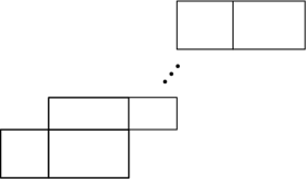
Figure 1. Rectangles $P_{0},\dots,P_{g-1}$ if $g$ is even.

Next, assume that $g$ is odd. Let $P_{0},\dots,P_{g-1}$ be rectangles satisfying the following:

• $P_{i}$ has a horizontal side for all $i=0,\dots,g-1$,

• $P_{0}$ is a square,

• $w(P_{2i})=w(P_{2i+1})$ for all $i=0,1,\dots,\frac{g-3}{2}$,

• $P_{2i}$ and $P_{2i+1}$ have a common horizontal side and $P_{2i}$ is below $P_{2i+1}$ for all $i=0,1,\dots,\frac{g-3}{2}$,

• $h(P_{2i-1})=h(P_{2i})$ for all $i=1,2,\dots,\frac{g-2}{2}$,

• $P_{2i-1}$ and $P_{2i}$ have common vertical side and $P_{2i-1}$ is on the left of $P_{2i}$ for all $i=1,2,\dots,\frac{g-2}{2}$

(see Figure2).

0pt $P_{0}$ at 45 45 $P_{1}$ at 45 114 $P_{2}$ at 154 114 $P_{3}$ at 154 161 $P_{g-2}$ at 333 224 $P_{g-1}$ at 333 276

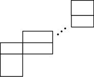
Figure 2. Rectangles $P_{0},\dots,P_{g-1}$ if $g$ is odd.

Let $g\geq 2$ and $P_{0},P_{1},\dots,P_{g-1}$ as above. Let $l$ be the line passing through the upper left vertex and the lower right vertex of $P_{0}$. Denote by $r_{l}$ the reflection about the line $l$. We set $Q_{i}=r_{l}(P_{i})$ for $i=1,2,\dots,g-1$ and

$$P=P_{0}\cup\bigcup_{i=1}^{g-1}\left(P_{i}\cup Q_{i}\right).$$

We make pairs of sides of $P$. Each side of $P$ is paired with its “opposite” side. For example, if $g\geq 4$ is even, the left side of $P_{2i}$ and the right side of $P_{2i+1}$ are pair for all $i=0,1,\dots,\frac{g-2}{2}$ and the lower side of $P_{2i-1}$ and the upper side of $P_{2i}$ are pair for all $i=1,2,\dots,\frac{g-2}{2}$. Identifying all pairs of sides of $P$ by parallel translation, we obtain a closed surface $X$ of genus $g$. We induce a complex structure of $X$ so that the polygon $P$ gives one of the chars. Then, $X$ is a Riemann surface of genus $g$.

2.2. Algebraic equations of the Riemann Surfaces $X$

Let $g\geq 2$ and $P$, $X$ as in subsection 2.1. In this subsection, we give an algebraic equation of the Riemann surface $X$. We use the following notations.

Notation 2.1.

We name some points of $P$ and $X$ as follows (see Figure 3);

• $o$ is the upper right vertex of $P_{g-1}$,

• $o^{\prime}$ is the lower left vertex of $Q_{g-1}$,

• $p_{i}$ is the center of $P_{j}$ for $j=0,1,\dots,g-1$,

• $q_{i}$ is the center of $Q_{j}$ for $j=1,2,\dots,g-1$,

• if $g$ is even, then $p_{g}$ is the midpoint of the upper side of $P_{g-1}$,

• if $g$ is even, then $q_{g}$ is the midpoint of the left side of $Q_{g-1}$,

• if $g$ is odd, then $p_{g}$ is the midpoint of the right side of $P_{g-1}$,

• if $g$ is odd, then $q_{g}$ is the midpoint of the lower side of $Q_{g-1}$, and

• we use the same symbols to the points on $X$ corresponding to the above points.

Note that $o$ and $o^{\prime}$ coincide on $X$. We denote the point of $X$ by $o$.

0pt $p_{0}$ at 93 317 $p_{1}$ at 203 317 $p_{2}$ at 203 379 $p_{3}$ at 330 379 $p_{4}$ at 330 420 $o$ at 415 415 $q_{1}$ at 130 200 $q_{2}$ at 50 200 $q_{3}$ at 50 80 $q_{4}$ at -16 80 $o^{\prime}$ at -15 5

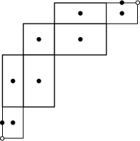
Figure 3. The points $p_{0},\dots,p_{g},q_{1},\dots,q_{g},o$ and $o^{\prime}$ if $g=4$.

Let $l$ be the line as in subsection 2.1 and $r_{l}$ the reflection about $l$. This reflection $r_{l}$ induces an antiautomorphism $\mu$ of $X$. Moreover, we can construct an automorphism $\tau$ of $X$ from the $\frac{\pi}{2}$-rotation about $p_{0}$. Let $P^{\prime}$ be the image of $P$ by this rotation. Then $P^{\prime}$ does not coincide with $P$. However, we can reconstruct $P$ from $P^{\prime}$. We cut $P^{\prime}$ along all sides which are shared by two of $P_{0},P_{1},\dots,P_{g-1},Q_{1},\dots,Q_{g-1}$ and glue the rectangles by the identification of sides of $P$. Then the resulting polygon is $P$ with the identification of the opposite sides. Thus, we obtain an automorphism $\tau$ of $X$. For the maps $\tau$ and $\mu$, we have the following.

Proposition 2.2.

The antiautomorphism $\mu$ is of order $2$. The automorphism $\tau$ is of order $4$. Moreover, $\mu^{2}$ is the hyperelliptic involution of $X$.

Proof.

The orders of $\tau$ and $\mu$ is clearly $2$ and $4$, respectively. We show that $\mu^{2}$ is the hyperelliptic involution of $X$. By construction, $\mu^{2}$ maps each $P_{i}$ and $Q_{j}$ to itself. Since $\mu^{2}$ acts on $P_{i}$ as $\pi$-rotation for each $i=0,1,\dots,g-1$, $\mu^{2}$ fixes the center $p_{i}$ of $P_{i}$. Moreover, $\mu^{2}$ fixes $p_{g}$. By the same argument, $\mu^{2}$ fixes $q_{1},q_{2},\dots,q_{g-1}$ and $q_{g}$. Finally, $\mu^{2}$ fixes $o$. Therefore, $\mu^{2}$ has $2g+2$ fixed points. This means that $\mu^{2}$ is the hyperelliptic involution of $X$. ∎

We now describe $X$ as an algebraic curve.

Theorem 2.3.

The Riemann surface $X$ is the algebraic curve defined by

$$w^{2}=z(z^{2}-1)(z^{2}-a_{1}^{2})\dots(z^{2}-a_{g-1}^{2}).$$

Here, $a_{1},\dots,a_{g-1}$ are real number satisfying $1<a_{1}<a_{2}<\cdots<a_{g-1}$. Moreover, we have $p_{0}=(0,0),p_{1}=(1,0),p_{j+1}=(a_{j},0),q_{1}=(-1,0),q_{j+1}=(-a_{j},0)$ for all $j=1,\dots,g-1$. Let $(z,w)$ be a point of the algebraic curve $X$. Then, we have $\tau(z,w)=(-z,iw)$ and $\mu(z,w)=(-\bar{z},-i\bar{w})$.

Remark.

Hereafter, we choose a branch of the square root so that $\sqrt{-x}=-i\sqrt{x}$ holds for all $x>0$.

To prove Theorem 2.3, we show the following lemma.

Lemma 2.4.

Let $f(x)$ be a real valued function defined on an interval $I$. Assume that the function $\frac{1}{\sqrt{f(x)}}:I\to\hat{\mathbb{R}}$ is integrable on $I$. Then, we have

$$\int_{I}\dfrac{dx}{\sqrt{-f(x)}}=i\cdot\overline{\int_{I}\frac{dx}{\sqrt{f(x)}}}.$$

Proof.

Set $I_{1}=\left\{x\in I:f(x)\geq 0\right\}$ and $I_{2}=\left\{x\in I:f(x)<0\right\}$. Then the integral $\displaystyle\int_{I_{1}}\frac{dx}{\sqrt{f(x)}}$ is a real number and $\displaystyle\int_{I_{2}}\frac{dx}{\sqrt{f(x)}}$ is a pure imaginary number. Moreover, the equation

$$-i\int_{I_{2}}\frac{dx}{\sqrt{f(x)}}=-i\int_{I_{2}}\frac{dx}{-i\sqrt{-f(x)}}=\int_{I_{2}}\frac{dx}{\sqrt{-f(x)}}$$

holds. Therefore, we have

$$\int_{I}\dfrac{dx}{\sqrt{-f(x)}} =\int_{I_{1}}\dfrac{dx}{\sqrt{-f(x)}}+\int_{I_{2}}\dfrac{dx}{\sqrt{-f(x)}}$$

$$=\int_{I_{1}}\dfrac{dx}{-i\sqrt{f(x)}}-i\int_{I_{2}}\frac{dx}{\sqrt{f(x)}}$$

$$=i\int_{I_{1}}\dfrac{dx}{\sqrt{f(x)}}-i\int_{I_{2}}\frac{dx}{\sqrt{f(x)}}$$

$$=i\left(\int_{I_{1}}\dfrac{dx}{\sqrt{f(x)}}-\int_{I_{2}}\frac{dx}{\sqrt{f(x)}}\right)$$

$$=i\cdot\overline{\int_{I}\frac{dx}{\sqrt{f(x)}}}.\qed$$

Proof of Theorem 2.3.

By Proposition 2.2, $\tau^{2}$ is the hyperelliptic involution of $X$ and $Y=X/\langle\tau^{2}\rangle$ is the Riemann sphere. Let $\varphi:X\to Y=\hat{\mathbb{C}}$ be the natural projection. We may assume that $\varphi(p_{0})=0$, $\varphi(p_{1})=1$ and $\varphi(o)=\infty$. The automorphism $\tau$ of $X$ induces an automorphism $\tau^{\prime}$ of $Y$. The automorphism $\tau^{\prime}$ is of order $2$ and fixes $\varphi(p_{0})=0$ and $\varphi(o)=\infty$. Hence, $\tau^{\prime}$ is the Möbius transformation which is of the form $\tau^{\prime}(z)=-z$. From this, we have $\varphi(p_{j})=-\varphi(q_{j})$ for all $j=1,2,\dots,g$. Since $\mu\tau^{2}=\tau^{2}\mu$ holds, the antiautomorphism $\mu$ of $X$ induces an automorphism $\mu^{\prime}$ of $Y$. The antiautomorphism $\mu^{\prime}$ is of order $2$ and fixes $\varphi(p_{0})=0$ and $\varphi(o)=\infty$. Moreover, $\mu^{\prime}$ maps $\varphi(p_{1})=1$ to $\varphi(q_{1})=-1$. Therefore, $\tau^{\prime}$ is the antiautomorphism which is of the form $\mu^{\prime}(z)=-\bar{z}$. For each $j=2,3,\dots,g-1$, we have

$$\varphi(p_{j})=-\varphi(q_{j})=-\varphi(\mu(p_{j}))=-\mu^{\prime}(\varphi(p_{j}))=\overline{\varphi(p_{j})}.$$

This implies that $\varphi(p_{j})$ is a real number for each $j=2,3,\dots,g-1$. We set $a_{j-1}=\varphi(p_{j})$ for each $j=2,3,\dots,g-1$. Now, $X$ is described by the algebraic equation

$$w^{2}=z(z^{2}-1)(z^{2}-a_{1}^{2})(z^{2}-a_{2}^{2})\cdots(z^{2}-a_{g-1}^{2}).$$

Next, we show that $1<a_{1}<a_{2}<\cdots<a_{g-1}$ holds. Set $f(z)=z(z^{2}-1)(z^{2}-a_{1}^{2})(z^{2}-a_{2}^{2})\cdots(z^{2}-a_{g-1}^{2})$. Assume that the polygon $P$ is in the $z$-plane. Let $\omega$ be the holomorphic $1$-form on $X$ induced by the $1$-form $dz$ on the polygon $P$. The $1$-form $\omega$ has a unique zero $o$ of order $2g-2$. The holomorphic $1$-form $\frac{dz}{w}$ is also has a unique zero $o$ since $o$ corresponds to $\infty$ via $\varphi$. There exists a constant $c\in\mathbb{C}^{\ast}$ such that $\omega=c\frac{dz}{w}$ holds. Let $\zeta$ be a local coordinate system of $X$ induced by ${\mathrm{Int}}(P)$. We may assume that $\zeta(p_{0})=0$. We describe points $p\in X$ by $(z,w)\in\mathbb{C}^{2}$ satisfying the above equation. Then, for sufficiently small neighborhood $U$ of $p_{0}$, the local coordinate system $\zeta$ is represented by

$$\zeta(p)=\int_{p_{0}}^{p}\omega=\int_{(0,0)}^{(z,w)}c\frac{dz}{w}=c\int_{0}^{z}\frac{dz}{\sqrt{f(z)}}.$$

Let $C$ be a lift of the real axis via the projection $\varphi:X\to X/\langle\tau^{2}\rangle$. Let $F:C\to\mathbb{C}$ be the analytic continuation of $\zeta$ along $C$. If $g$ is even, we have

$$|p_{0}p_{1}|=\int_{p_{0}}^{p_{1}}\omega=c\int_{0}^{1}\frac{dz}{\sqrt{f(z)}}.$$

Moreover, by Lemma 2.4,

$$|p_{0}p_{1}|=|p_{0}q_{1}| =i\int_{p_{0}}^{q_{1}}\omega=ic\int_{0}^{-1}\frac{dz}{\sqrt{f(z)}}=ic\int_{0}^{1}\frac{-dz}{\sqrt{-f(x)}}=c\cdot\overline{\int_{0}^{1}\frac{dz}{\sqrt{f(z)}}.}$$

Therefore, $\displaystyle\int_{0}^{1}\frac{dz}{\sqrt{f(z)}}$ and $c$ are real numbers. If there exists $l\in\left\{1,2,\dots,g-1\right\}$ such that $0<|a_{l}|<1$, the integral $\displaystyle\int_{0}^{1}\frac{dz}{\sqrt{f(z)}}$ is not real. Thus, $1<|a_{l}|$ holds for all $l\in\left\{1,2,\dots,g-1\right\}$ . Let $C_{0}$ be the path from $p_{0}$ to $p_{1}$ along $C$. Then $F(C)$ is a horizontal segment $p_{0}p_{1}$ in $P$. Moreover, the image $F(C)$ consists of horizontal segments and vertical segments. This implies that $F(C)$ pass through $p_{0},p_{1},\dots,p_{g},o$ in this order. Therefore, we have $1<a_{1}<a_{2}<\cdots<a_{g-1}$. If $g$ is odd, by the same way, we can see that $\displaystyle\int_{0}^{1}\frac{dz}{\sqrt{f(z)}}$ is a pure imaginary number, $c$ is a real number and hence, $1<a_{1}<a_{2}<\cdots<a_{g-1}$ holds.

Finally, we show $\tau(z,w)=(-z,iw)$ and $\mu(z,w)=(-\bar{z},-i\bar{w})$ for all $(z,w)\in X$. Since $\tau^{\prime}(z)=-z$ holds, the first coordinate of $\tau(z,w)$ is $-z$. The equation $f(-z)=-f(z)=-w^{2}$ implies that the second coordinate of $\tau(z,w)$ is $\pm iw$. We set $\tau(z,w)=(-z,\varepsilon iw)$. Then, $\int_{\tau(C_{0})}\omega=i|p_{0}q_{1}|=i|p_{0}p_{1}|$ and

$$\int_{\tau(C_{0})}\omega=\int_{\tau(C_{0})}c\frac{dz}{w}=\int_{C_{0}}\tau^{\ast}\left(c\frac{dz}{w}\right)=\int_{C_{0}}c\frac{-dz}{i\varepsilon w}=\frac{i}{\varepsilon}\int_{C_{0}}c\frac{dz}{w}=\frac{i}{\varepsilon}|p_{0}p_{1}|$$

hold. Hence, we have $\varepsilon=1$ and $\tau(z,w)=(-z,iw)$ for all $(z,w)\in X$. ∎

2.3. Representation of Algebraic Curves by Polygon

In subsection 2.1, we show that the Riemann surface which is obtained from the polygon $P$ is the algebraic curve defined by

$$w^{2}=z(z^{2}-1)(z^{2}-a_{1}^{2})(z^{2}-a_{2}^{2})\cdots(z^{2}-a_{g-1}^{2})$$

for some $a_{1},a_{2},\dots,a_{g-1}$ ($1<a_{1}<a_{2}<\cdots<a_{g-1}$). In this subsection, we show the following.

Theorem 2.5.

Let $g\geq 2$. For all $a_{1},a_{2},\dots,a_{g-1}$ ($1<a_{1}<a_{2}<\cdots<a_{g-1}$), the algebraic curve

$$w^{2}=z(z^{2}-1)(z^{2}-a_{1}^{2})(z^{2}-a_{2}^{2})\cdots(z^{2}-a_{g-1}^{2})$$

is obtained from the polygon

$$P=P_{0}\cup\bigcup_{i=1}^{g-1}\left(P_{i}\cup Q_{i}\right)$$

as in Figure 1 or Figure 2 by adjusting the lengths of rectangles. Here, $P_{0}$ is a square.

We prove this theorem by the theory of translation surfaces. Hereafter, we assume that $X$ is a compact Riemann surface of genus $g\geq 2$.

Definition 2.6 (Translation Surface).

A translation surface $(X,\omega)$ is a pair of a Riemann surface $X$ and a non-zero holomorphic $1$-form $\omega$ on $X$. The zeros of $\omega$ are called singular points of the translation surface $(X,\omega)$. Denote by $\mathrm{Zero}(\omega)$ the set of all zeros of $\omega$.

Let $\omega$ be a non-zero holomorphic $1$-form $\omega$ on $X$. If $p_{0}\in X$ is not a zero of $\omega$, there is a neighborhood $U$ such that

$$z=\int_{p_{0}}^{p}\omega:U\rightarrow\mathbb{C}$$

is a chart of $X$. Let $(U,z)$ and $(V,w)$ be such charts with $U\cap V\not=\emptyset$. The transition function is of the form $w=z+(\mbox{const.})$. Hence, $(X,\omega)$ is a surface with a Euclidean structure on $X-\mathrm{Zero}(\omega)$. If $p_{0}$ is a zero of $\omega$ of order $n$, there exists a chart $\zeta:U\to\mathbb{C}$ of $X$ such that $\zeta(p_{0})=0$ $\omega=\zeta^{n}d\zeta$. Then,

$$z=\int_{p_{0}}^{p}\omega=\frac{1}{n+1}\zeta^{n+1}:U\rightarrow\mathbb{C}$$

is a chart around $p_{0}$. With respect to this chart, the angle around $p_{0}$ is $2\pi(n+1)$.

We define some terminologies for translation surfaces. Let $(X,\omega)$ be a translation surface. We consider geodesics with respect to the Euclidean structure on $(X,\omega)$.

Definition 2.7 (Saddle connection).

A saddle connection of a translation surface $(X,\omega)$ is a geodesic segment on $(X,\omega)$ whose end points are singular points and containing no singular points in its interior. Note that the end points of a saddle connection may be same.

For closed geodesics on translation surfaces, we have the following.

Proposition 2.8.

Let $\gamma$ be a closed geodesic on a translation surface $(X,\omega)$. Then, one of the following two holds;

1. $\gamma$ contains no singular points,

2. $\gamma$ is a concatenation of saddle connections. Assume that $\gamma$ passes a saddle connection $s_{2}$ just after a saddle connection $s_{1}$ and the switch occurs at a singular point $p_{0}$. The angles at $p_{0}$ in both sides of $s_{1}\cup s_{2}$ are greater than or equal to $\pi$.

Definition 2.9.

Let $\gamma$ be a closed geodesic on a translation surface $(X,\omega)$ which does not contain singular points. The geodesic $\gamma$ is horizontal (resp. vertical) if it is horizontal (resp. vertical) with respect to the Euclidean structure of $(X,\omega)$.

We construct polygon $P$ as in Theorem 2.5 from horizontal and vertical closed geodesics. Then, we use maximal cylinders for the geodesics.

Definition 2.10 (Maximal Cylinder).

Let $\gamma$ be a closed geodesic on a translation surface $(X,\omega)$ which does not contain singular points. The maximal cylinder $R_{\gamma}$ for $\gamma$ is the union of all closed geodesics on $(X,\omega)$ which do not contain singular points and are homotopic to $\gamma$.

By Definition 2.10, we have the following.

Proposition 2.11.

Let $\gamma$ be a closed geodesic on a translation surface $(X,\omega)$ which does not contain singular points. The maximal cylinder $R_{\gamma}$ for $\gamma$ is a cylinder each of whose boundary components are closed geodesics constructed from saddle connections that are parallel to $\gamma$.

We now prove Theorem 2.5. Choose $a_{1},a_{2},\dots,a_{g-1}$ so that $1<a_{1}<a_{2}<\cdots<a_{g-1}$ and set $f(z)=w^{2}=z(z^{2}-1)(z^{2}-a_{1}^{2})(z^{2}-a_{2}^{2})\cdots(z^{2}-a_{g-1}^{2})$. Let $X$ be the algebraic curve $w^{2}=f(z)$ and $\varphi:X\to\hat{\mathbb{C}};(z,w)\mapsto z$ the natural projection. Set $o=\varphi^{-1}(\infty)$. The algebraic curve $X$ has an automorphism $\tau:X\to X;(z,w)\to(-z,iw)$ . The map $\tau$ is of order $4$ and $\tau^{2}$ is the hyperelliptic involution of $X$. The fixed points of $\tau^{2}$ are $(0,0),(\pm 1,0),(\pm a_{1},0),(\pm a_{2},0),\dots,(\pm a_{g-1},0)$ and $o$. Let $\delta_{0},\delta_{1},\dots,\delta_{g-1}$ be preimages of the intervals $[0,1],[1,a_{1}],[a_{1},a_{2}],\dots,[a_{g-2},a_{g-1}]$, respectively. Set $\delta_{j}^{\ast}=\tau(\delta_{j})$ for each $j=0,1,\dots,g-1$. Then $\delta_{j}$ and $\delta_{j}^{\ast}$ are simple closed curves on $X$.

Let $i(\cdot,\cdot)$ be the geometric intersection number function. By construction, we have the following proposition.

Proposition 2.12.

The following holds.

1. For any $j=0,1,\dots,g-2$, $i(\delta_{j},\delta_{j+1})=1$ holds. The curves $\delta_{j}$ and $\delta_{j+1}$ intersect only at $(a_{j},0)$. If $|j-k|\not=1$ then $i(\delta_{j},\delta_{k})=0$ holds.

2. For any $j=0,1,\dots,g-2$, $i(\delta_{j}^{\ast},\delta_{j+1}^{\ast})=1$ holds. The curves $\delta_{j}^{\ast}$ and $\delta_{j+1}^{\ast}$ intersect only at $(-a_{j},0)$. If $|j-k|\not=1$ then $i(\delta_{j}^{\ast},\delta_{k}^{\ast})=0$ holds.

3. The equation $i(\delta_{0},\delta_{0}^{\ast})=1$ holds. The curves $\delta_{0}$ and $\delta_{0}^{\ast}$ intersect only at $(0,0)$. If $(j,k)\not=(0,0)$, then $i(\delta_{j},\delta_{k}^{\ast})=0$ holds.

Set $\omega_{0}=\dfrac{dz}{w}$. The holomorphic differential $\omega_{0}$ has a unique zero at $o$. Therefore, $o$ is the unique singular point of the translation surface $(X,\omega_{0})$. The angle around $o$ is $2\pi(2g-1)$ on $(X,\omega_{0})$. Moreover, we have the following proposition.

Proposition 2.13.

The simple closed curves $\delta_{0},\dots,\delta_{g-1},\delta_{0}^{\ast},\dots,\delta_{g-1}^{\ast}$ are closed geodesics on the translation surface $(X,\omega_{0})$. If $g$ is even, then $\delta_{0}$, $\delta_{2}$, $\dots$, $\delta_{g-2}$, $\delta_{1}^{\ast}$, $\delta_{3}^{\ast}$, $\dots$, $\delta_{g-1}^{\ast}$ are horizontal and $\delta_{1}$, $\delta_{3}$, $\dots$, $\delta_{g-1}$, $\delta_{0}^{\ast}$, $\delta_{2}^{\ast}$, $\dots$, $\delta_{g-2}^{\ast}$ are vertical on $(X,\omega_{0})$. If $g$ is odd, then $\delta_{0}$, $\delta_{2}$, $\dots$, $\delta_{g-2}$, $\delta_{1}^{\ast}$, $\delta_{3}^{\ast}$, $\dots$, $\delta_{g-1}^{\ast}$ are vertical and $\delta_{1}$, $\delta_{3}$, $\dots$, $\delta_{g-1}$, $\delta_{0}^{\ast}$, $\delta_{2}^{\ast}$, $\dots$, $\delta_{g-2}^{\ast}$ are horizontal on $(X,\omega_{0})$.

Proof.

We prove the case if $g$ is even. Since $f(t)>0$ holds for any $t\in(0,1)$, $\int_{0}^{t}\frac{dz}{\sqrt{f(z)}}>0$ holds. Hence, $\delta_{0}$ is a horizontal closed geodesic on $(X,\omega_{0})$. Since $f(t)<0$ holds for any $t\in(1,a_{1})$, $\int_{1}^{t}\frac{dz}{\sqrt{f(z)}}\in i\mathbb{R}$ holds. Hence, $\delta_{1}$ is a vertical closed geodesic on $(X,\omega_{0})$. We can prove the others by the same way. ∎

Let $\nu:X\to X;(z,w)\mapsto(\bar{z},(-1)^{g}\bar{w})$ be an antiautomorphism of $X$. Set $R_{j}=R_{\delta_{j}}$ and $R_{j}^{\ast}=R_{\delta_{j}^{\ast}}$ (see Definition 2.10). We regard each boundary component of the cylinder $R_{j}$ (resp. $R_{j}^{\ast}$) as a closed curve which is homotopic to $\delta_{j}$ (resp. $\delta_{j}^{\ast}$). We denote the boundary components by $\partial_{1}R_{j}$ and $\partial_{2}R_{j}$ (resp. $\partial_{1}R_{j}^{\ast}$ and $\partial_{2}R_{j}^{\ast}$).

Lemma 2.14.

For any $j=0,1,\dots,g-1$, we have the following;

1. $\tau(R_{j})=R_{j}^{\ast}$ and $\tau(R_{j}^{\ast})=R_{j}$ holds.

2. The simple closed geodesics $\delta_{j}$ and $\delta_{j}^{\ast}$ are invariant under $\tau^{2}$, respectively. Two boundary components $\partial_{1}R_{j}$ and $\partial_{2}R_{j}$ (resp. $\partial_{1}R_{j}^{\ast}$ and $\partial_{2}R_{j}^{\ast}$) are permuted by $\tau^{2}$.

3. Simple closed geodesics $\delta_{j}$ and $\delta_{j}^{\ast}$ are invariant under $\nu$, respectively. The geodesic $\delta_{j}$ is pointwise fixed by $\nu$ if and only if $j$ is even. Then, $\nu$ is represented as the reflection about $\delta_{j}$ in a sufficiently small neighborhood of $\delta_{j}$. The geodesic $\delta_{j}^{\ast}$ is pointwise fixed by $\nu$ if and only if $j$ is odd. Then, $\nu$ is represented as the reflection about $\delta_{j}^{\ast}$ in a sufficiently small neighborhood of $\delta_{j}^{\ast}$.

4. The cylinders $R_{j},R_{j}^{\ast}$ are invariant under $\nu$, respectively. If $j$ is even, then two boundary components $\partial_{1}R_{j}$ and $\partial_{2}R_{j}$ are permuted by $\nu$ and each boundary component of $R_{j}^{\ast}$ are invariant under $\nu$. If $j$ is odd, then two boundary components $\partial_{1}R_{j}^{\ast}$ and $\partial_{2}R_{j}^{\ast}$ are permuted by $\nu$ and each boundary component of $R_{j}$ are invariant under $\nu$.

Proof.

1. Since $\delta_{j}^{\ast}=\tau(\delta_{j})$, we obtain the claim.

2. Since $\tau^{\ast}\dfrac{dz}{w}=i\dfrac{dz}{y}$ holds, the automorphism $\tau$ acts on $(X,\omega_{0})$ as $\frac{\pi}{2}$-rotation. The closed geodesic $\delta_{j}$ passes through two fixed points of $\tau^{2}$. Hence, $\delta_{j}$ is invariant under $\tau^{2}$ and two boundary components of $R_{j}$ are permuted by $\tau^{2}$. By the same argument as above, $\delta_{j}^{\ast}$ is invariant under $\tau^{2}$ and two boundary components of $R_{j}^{\ast}$ are permuted by $\tau^{2}$.

3. We prove the case where $g$ is even. The case where $g$ is odd is proved by the same way. Assume that $g$ is even. Since $\nu^{\ast}\left(\dfrac{dz}{w}\right)=\overline{\left(\dfrac{dz}{w}\right)}$ holds, $\nu$ preserves horizontal slopes and vertical slopes of segments on $(X,\omega_{0})$. The geodesic $\delta_{j}$ passes through $(a_{j-1},0)$ and $(a_{j},0)$ which are fixed points of $\nu$. Thus, $\delta_{j}$ is invariant under $\nu$. By the same argument, $\delta_{j}^{\ast}$ is invariant under $\nu$. Moreover, the set of all fixed points of $\nu$ is

   $$\left\{(z,w)\in X:z,w\in\mathbb{R}\right\}=\delta_{0}\cup\delta_{2}\cup\dots\cup\delta_{g-2}\cup\delta_{1}^{\ast}\cup\delta_{3}^{\ast}\cup\dots\cup\delta_{g-1}^{\ast}.$$

   Therefore, we obtain the claim.

4. It is clear by (3).

∎

Lemma 2.15.

For any $k=1,2$ and $j=0,1,\dots,g-1$, the boundary component $\partial_{k}R_{j}$ passes through the singular point $o$ of $(X,\omega_{0})$ at least twice.

Proof.

By construction, the curve $\partial_{k}R_{j}$ passed through $o$ at least once. Let $s^{\prime}$ be a perpendicular segment from $o$ to $\delta_{j}$ in $R_{j}$. If $j$ is even, we set $s=s^{\prime}\cup\nu(s^{\prime})$. If $j$ is odd, we set $s=\tau^{-1}\left(\tau(s^{\prime})\cup\nu\tau(s^{\prime})\right)=s^{\prime}\cup\tau^{-1}\nu\tau(s^{\prime})$. I both cases, $s$ is a segment whose end points are $o$ and which is orthogonal to $\delta_{j}$. We show that $s$ is not invariant under $\tau^{2}$. If $s$ is invariant under $\tau^{2}$, then the midpoint of $s$, say $p$, is a fixed point of $\tau^{2}$. Thus $p=(a_{j-1},0)$ or $(a_{j},0)$. Here, we set $a_{-1}=0$, $a_{0}=1$. If $p=(a_{j-1},0)$, then $s$ is contained in $\delta_{j-1}$. This contradicts that $\delta_{j-1}$ does not pass through $o$. If $p=(a_{j},0)$, then $s$ is contained in $\delta_{j+1}$. This contradicts that $\delta_{j+1}$ does not pass through $o$. Therefore, $s$ is not invariant under $\tau^{2}$ and $\tau^{2}(s)\neq s$ holds. Now, $\tau^{2}(s)$ is a segment connecting two boundaries $\partial_{1}R_{j}$ and $\partial_{2}R_{j}$ in $R_{j}$ and whose end points are $o$. Thus, we obtain the claim. ∎

Proof of Theorem 2.5.

Let $c_{j}$ be the number of times that the boundary component $\partial_{1}R_{j}$ passes through the singular point $o$ of $(X,\omega_{0})$ for each $j=0,1,\dots,g-1$. Then $\partial_{2}R_{j},\partial_{1}R_{j}^{\ast}$ and $\partial_{2}R_{j}^{\ast}$ pass through $o$ just $c_{j}$ times, respectively. Set $L_{j}={\mathrm{Int}}(R_{j})\cap{\mathrm{Int}}(R_{j+1})$ for $j=0,1,\dots,g-2$. Then $L_{j}$ is a rectangle in $(X,\omega_{0})$. By Lemma 2.14 (2) and (4), $L_{j}$ is invariant under $\tau^{2}$ and $\nu$. This implies that if one of the vertices of $L_{j}$ is $o$, then all vertices are $o$. It is also true for rectangles $L={\mathrm{Int}}(R_{0})\cap{\mathrm{Int}}(R_{0}^{\ast})$ and $L_{j}^{\ast}={\mathrm{Int}}(R_{j}^{\ast})\cap{\mathrm{Int}}(R_{j+1}^{\ast})$ for $j=0,1,\dots,g-2$. Assume that $d$ of $L,L_{0},\dots,L_{g-2},L_{0}^{\ast},\dots,L_{g-2}^{\ast}$ have $o$ as their vertices. Since the angle around $o$ in $(X,\omega_{0})$ is $(4g-2)\pi$, the inequality

$$2\sum_{j=0}^{g-1}2\pi c_{j}-2\pi d\leq(4g-2)\pi$$

holds. Since $c_{j}\geq 2$ for all $j=0,1,\dots,g-2$ by Lemma 2.15, we have

$$2g-3+2c_{g-1}\leq d.$$

Since $d\leq 2g-1$ by definition, we obtain $c_{g-1}=1$, $d=2g-1$ and $c_{j}=2$ for all $j=0,1,\dots,g-2$. This implies that $\partial_{k}R_{j}$ (resp. $\partial_{k}R_{j}^{\ast}$ ) passes through the singular point $o$ just twice for all $j=1,2,\dots,g-2$ and $k=1,2$ and all vertices of rectangles $L,L_{0},\dots,L_{g-2},L_{0}^{\ast},\dots,L_{g-2}^{\ast}$ are the singular point $o$. Therefore, we have

$$X=\overline{L}\cup\bigcup_{j=0}^{g-2}\overline{L_{j}}\cup\bigcup_{j=0}^{g-2}\overline{L_{j}^{\ast}}.$$

Moreover, since $L$ is invariant under $\tau$, $L$ is a square. ∎

Corollary 2.16.

Let $g\geq 2$. Let $a_{1},a_{2},\dots,a_{g-1}\in\mathbb{R}$ with $1<a_{1}<a_{2}<\cdots<a_{g-1}$ and set $a_{-1}=0$, $a_{0}=1$, $a_{g}=\infty$ and $f(z)=z(z^{2}-1)(z^{2}-a_{1}^{2})\cdots(z^{2}-a_{g-1}^{2})$. We also set

$$I_{j}=\int_{a_{j-1}}^{a_{j}}\dfrac{dz}{\sqrt{|f(z)|}}$$

for $j=0,1,\dots,g$. Then the equation

$$\sum_{j=0}^{g}(-1)^{[\frac{j+1}{2}]}I_{j}=0$$

holds.

Proof.

Here, we prove the case where $g$ is even. By Theorem 2.5, the algebraic curve $X$ defined by $w^{2}=f(z)$ is obtained from the polygon

$$P=P_{0}\cup\bigcup_{i=1}^{g-1}\left(P_{i}\cup Q_{i}\right)$$

as in Figure 1 by adjusting the lengths of rectangles. Here, $P_{0}$ is a square. The length of horizontal edge of $L$ is represented by

$$2\left(I_{0}-I_{2}+\cdots+(-1)^{[\frac{g-1}{2}]}I_{g-2}+(-1)^{[\frac{g+1}{2}]}I_{g}\right).$$

The length of vertical edge of $L$ is represented by

$$2\left(I_{1}-I_{3}+\dots+(-1)^{[\frac{g-4}{2}]}I_{g-3}+(-1)^{[\frac{g-2}{2}]}I_{g-1}\right)$$

Since $L$ is a square, we have

$$I_{0}-I_{2}+\cdots+(-1)^{[\frac{g-1}{2}]}I_{g-2}+(-1)^{[\frac{g+1}{2}]}I_{g}$$

$$= I_{1}-I_{3}+\dots+(-1)^{[\frac{g-4}{2}]}I_{g-3}+(-1)^{[\frac{g-2}{2}]}I_{g-1}$$

From this, we obtain the claim. ∎

3. Calculation of Period Matrices

3.1. Construction of symplectic bases

Let $g\geq 2$. In this section, we construct a symplectic basis of our algebraic curve $X$ defined by $w^{2}=z(z^{2}-1)(z^{2}-a_{1}^{2})\cdots(z^{2}-a_{g-1}^{2})$ ($1<a_{1}<a_{2}<\cdots<a_{g-1}$). By Theorem 2.5, the algebraic curve $X$ is obtained from the polygon

$$P=P_{0}\cup\bigcup_{i=1}^{g-1}\left(P_{i}\cup Q_{i}\right)$$

as in Figure 1 or 2 by adjusting the lengths of rectangles. Since we construct a symplectic basis of $H_{1}(X,\mathbb{Z})$ by topological arguments, we may describe $P_{0}$, $P_{1}$,$\dots,P_{g-1}$, $Q_{1}$, $\dots,Q_{g-1}$ as unit squares. Let $\alpha_{1},\dots,\alpha_{g},\beta_{1},\dots,\beta_{g}$ be simple closed curves of $X$ as in Figure 4. That is, $\alpha_{1},\dots,\alpha_{g}$ are curves induced by horizontal segments passing through centers of the squares $P_{0}$, $P_{1}$,$\dots,P_{g-1}$, $Q_{1}$, $\dots,Q_{g-1}$ which are not homotopic to each other. We label $\alpha_{1},\dots,\alpha_{g}$ so that $\alpha_{i}$ is below $\alpha_{j}$ if $i<j$. The curves $\beta_{1},\dots,\beta_{g}$ are induced by vertical segments passing through centers of the squares $P_{0}$, $P_{1}$,$\dots,P_{g-1}$, $Q_{1}$, $\dots,Q_{g-1}$ which are not homotopic to each other. We label $\beta_{1},\dots,\beta_{g}$ so that $\beta_{i}$ is on the left side of $\beta_{j}$ if $i<j$.

0pt $\alpha_{1}$ at -25 53 $\alpha_{2}$ at -25 144 $\alpha_{3}$ at 75 234 $\alpha_{4}$ at 160 323 $\beta_{1}$ at 585 210 $\beta_{2}$ at 675 305 $\beta_{3}$ at 765 390 $\beta_{4}$ at 855 390

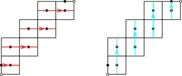
Figure 4. Simple closed curves $\alpha_{1},\dots,\alpha_{g},\beta_{1},\dots,\beta_{g}$.

We show the following.

Proposition 3.1.

Let $\alpha_{1},\dots,\alpha_{g},\beta_{1},\dots,\beta_{g}$ be simple closed curves defined as above. There exists a symplectic basis $\left\{\alpha_{1},\dots,\alpha_{g},\gamma_{1},\dots,\gamma_{g}\right\}$ of $H_{1}(X,\mathbb{Z})$ such that $\displaystyle\gamma_{j}=\sum_{k=j}^{g}(-1)^{k-j}\beta_{k}$ holds in $H_{1}(X,\mathbb{Z})$ for all $j=1,2,\dots,g$.

Proof.

If $g=2$, we define the simple closed curves $\gamma_{1}$ and $\gamma_{2}$ as in Figure 5. Then, $\gamma_{1}=\beta_{1}-\beta_{2}$ and $\gamma_{2}=\beta_{2}$ hold in $H_{1}(X,\mathbb{Z})$ and $\left\{\alpha_{1},\alpha_{2},\gamma_{1},\gamma_{2}\right\}$ is a symplectic basis of $H_{1}(X,\mathbb{Z})$.

0pt $\gamma_{1}$ at 36 202 $\gamma_{1}$ at 157 202 $\gamma_{2}$ at 118 202

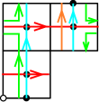
Figure 5. Simple closed curves $\gamma_{1}$ and $\gamma_{2}$ if $g=2$.

Next, we construct simple closed curves $\gamma_{1}$, $\gamma_{2}$ and $\gamma_{3}$ for the case where $g=3$. As in Figure 6, we glue a rectangle constructed by two unit squares with the polygon of Figure 5. We reconstruct $\gamma_{1}$ and $\gamma_{2}$ by gluing curves with the same colors as in Figure 6 and define $\gamma_{3}=\beta_{3}$. Then $\gamma_{1}=\beta_{1}-\beta_{2}+\beta_{3}$, $\gamma_{2}=\beta_{2}-\beta_{3}$ and $\gamma_{3}=\beta_{3}$ hold in $H_{1}(X,\mathbb{Z})$ and $\left\{\alpha_{1},\alpha_{2},\alpha_{3},\gamma_{1},\gamma_{2},\gamma_{3}\right\}$ is a symplectic basis of $H_{1}(X,\mathbb{Z})$ .

0pt $\gamma_{1}$ at 433 202 $\gamma_{1}$ at 562 295 $\gamma_{2}$ at 515 295 $\gamma_{2}$ at 652 295 $\gamma_{3}$ at 613 295 $\Rightarrow$ at 326 141

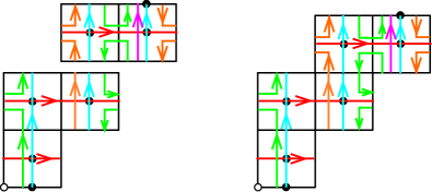
Figure 6. Simple closed curves $\gamma_{1}$, $\gamma_{2}$ and $\gamma_{3}$ if $g=3$

For the case where $g=4$, we glue a rectangle constructed by two unit squares with the right polygon of Figure 6 as in Figure 7. We reconstruct $\gamma_{1}$, $\gamma_{2}$ and $\gamma_{3}$ by gluing curves with the same colors as in Figure 7 and define $\gamma_{4}=\beta_{4}$. Then $\gamma_{1}=\beta_{1}-\beta_{2}+\beta_{3}-\beta_{4}$, $\gamma_{2}=\beta_{2}-\beta_{3}+\beta_{4}$, $\gamma_{3}=\beta_{3}-\beta_{4}$ and $\gamma_{4}=\beta_{4}$ hold in $H_{1}(X,\mathbb{Z})$ and $\left\{\alpha_{1},\alpha_{2},\alpha_{3},\alpha_{4},\gamma_{1},\gamma_{2},\gamma_{3},\gamma_{4}\right\}$ is a symplectic basis of $H_{1}(X,\mathbb{Z})$.

0pt $\gamma_{1}$ at 533 202 $\gamma_{1}$ at 690 379 $\gamma_{2}$ at 615 295 $\gamma_{2}$ at 752 379 $\gamma_{3}$ at 720 379 $\gamma_{3}$ at 835 379 $\gamma_{4}$ at 803 379 $\Rightarrow$ at 411 186

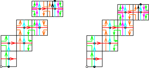
Figure 7. Simple closed curves $\gamma_{1}$, $\gamma_{2}$, $\gamma_{3}$ and $\gamma_{4}$ if $g=4$

Repeating this process, we can construct a symplectic basis $\left\{\alpha_{1},\dots,\alpha_{g},\gamma_{1},\dots,\gamma_{g}\right\}$ of $H_{1}(X,\mathbb{Z})$ satisfying the condition as in Proposition 3.1 for any $g\geq 2$. ∎

3.2. Period Matrices of $X$

Let $g\geq 2$ and $a_{1},a_{2},\dots,\alpha_{g-1}\in\mathbb{R}$ with $1<a_{1}<a_{2}<\cdots<a_{g-1}$. Set $f(z)=z(z^{2}-1)(z^{2}-a_{1}^{2})\cdots(z^{2}-a_{g-1}^{2})$. We calculate the period matrix of the algebraic curve $X$ defined by $w^{2}=f(z)$ for the symplectic basis $\left\{\alpha_{1},\dots,\alpha_{g},\gamma_{1},\dots,\gamma_{g}\right\}$ of $H_{1}(X,\mathbb{Z})$ which we construct in Proposition 3.1.

We recall some definitions and theorems. By Theorem 2.5, $X$ is obtained from the polygon $P$ as in Figure 1 or Figure 2. We define some points of $X$ and $P$ as Notation2.1. By Theorem 2.3, we have $p_{0}=(0,0),p_{1}=(1,0),p_{j+1}=(a_{j},0),q_{1}=(-1,0),q_{j+1}=(-a_{j},0)$ for all $j=1,\dots,g-1$. Moreover, $X$ has an automorphism $\tau(z,w)=(-z,iw)$ and antiautomorphism $\mu(z,w)=(-\bar{z},-i\bar{w})$. The actions of these maps are seen in subsection 2.1. Let $\alpha_{1},\dots,\alpha_{g},\beta_{1},\dots,\beta_{g}$ be curves defined in subsection 3.1 (see Figure 4). The curve $\gamma_{j}$ is defined by Proposition 3.1 so that $\displaystyle\gamma_{j}=\sum_{k=j}^{g}(-1)^{k-j}\beta_{k}$ holds in $H_{1}(X,\mathbb{Z})$ for all $j=1,2,\dots,g$. The family $\left\{\alpha_{1},\dots,\alpha_{g},\gamma_{1},\dots,\gamma_{g}\right\}$ is a symplectic basis of $H_{1}(X,\mathbb{Z})$.

To calculate the period matrix of $X$ for $\left\{\alpha_{1},\dots,\alpha_{g},\gamma_{1},\dots,\gamma_{g}\right\}$, we need a basis of the space $\Omega(X)$ of holomorphic $1$-forms on $X$. We set $\omega_{j}=\dfrac{z^{j-1}dz}{w}$ for all $j=1,2,\dots,g$. Then $\left\{\omega_{1},\omega_{2},\dots,\omega_{g}\right\}$ is a basis of $\Omega(X)$. Now we calculate the period matrix $\Pi$ of $X$ for the symplectic basis $\left\{\alpha_{1},\dots,\alpha_{g},\gamma_{1},\dots,\gamma_{g}\right\}$. We set

$$A=\left[\int_{\alpha_{k}}\frac{z^{j-1}dz}{w}\right],B=\left[\int_{\beta_{k}}\frac{z^{j-1}dz}{w}\right],C=\left[\int_{\gamma_{k}}\frac{z^{j-1}dz}{w}\right].$$

If $g$ is even, then we set

$$I_{j,k}=\left\{\begin{array}[]{ll}\displaystyle(-1)^{j-1}\int_{a_{g-2k}}^{a_{g-2k+1}}\dfrac{z^{j-1}dz}{\sqrt{|f(z)|}}&\left(1\leq k\leq\frac{g}{2}-1\right)\\ &\\ \displaystyle(-1)^{j-1}\int_{1}^{a_{1}}\dfrac{z^{j-1}dz}{\sqrt{|f(z)|}}&\left(k=\frac{g}{2}\right)\\ &\\ \displaystyle\int_{0}^{1}\dfrac{z^{j-1}dz}{\sqrt{|f(z)|}}&\left(k=\frac{g}{2}+1\right)\\ &\\ \displaystyle\int_{a_{2k-g-3}}^{a_{2k-g-2}}\dfrac{z^{j-1}dz}{\sqrt{|f(z)|}}&\left(\frac{g}{2}+2\leq k\leq g\right)\end{array}\right.$$

for all $j=1,2,\dots,g$. If $g$ is odd, then we set

$$I_{j,k}=\left\{\begin{array}[]{ll}\displaystyle(-1)^{j-1}\int_{a_{g-2k}}^{a_{g-2k+1}}\dfrac{z^{j-1}dz}{\sqrt{|f(z)|}}&\left(1\leq k\leq\frac{g-1}{2}\right)\\ &\\ \displaystyle(-1)^{j-1}\int_{0}^{1}\dfrac{z^{j-1}dz}{\sqrt{|f(z)|}}&\left(k=\frac{g+1}{2}\right)\\ &\\ \displaystyle\int_{1}^{a_{1}}\dfrac{z^{j-1}dz}{\sqrt{|f(z)|}}&\left(k=\frac{g+3}{2}\right)\\ &\\ \displaystyle\int_{a_{2k-g-3}}^{a_{2k-g-2}}\dfrac{z^{j-1}dz}{\sqrt{|f(z)|}}&\left(\frac{g+5}{2}\leq k\leq g\right)\end{array}\right.$$

for all $j=1,2,\dots,g$. In both cases, we set $\Pi_{0}=[I_{j,k}]$. Then, we have the following.

Lemma 3.2.

The equation

$$\int_{\alpha_{k}}\omega_{j}=2I_{j,k}$$

holds for any $j,k\in\left\{1,2,\dots,g\right\}$. Moreover, $A=2\Pi_{0}$ holds.

Proof.

We prove the case where $g$ is even. We can prove the case where $g$ is odd by the same argument. Suppose that $g$ is even. Let $\varphi:X\to\hat{\mathbb{C}}:(z,w)\to z$ be the natural projection. Then, we have

$$\varphi(\alpha_{k})=\left\{\begin{array}[]{ll}\left[-a_{g-2k+1},-a_{g-2k}\right]&\left(1\leq k\leq\frac{g}{2}-1\right)\\ &\\ \left[-a_{1},-1\right]&\left(k=\frac{g}{2}\right)\\ &\\ \left[0,1\right]&\left(k=\frac{g}{2}+1\right)\\ &\\ \left[a_{2k-g-3},a_{2k-g-2}\right]&\left(\frac{g}{2}+2\leq k\leq g\right)\end{array}\right.$$

for all $k=1,2,\dots,g$. If $1\leq k\leq\frac{g}{2}-1$, then

$$\int_{\alpha_{k}}\omega_{j}=2\int_{\varphi(\alpha_{k})}\dfrac{z^{j-1}dz}{\sqrt{|f(z)|}}=2\int_{-a_{g-2k+1}}^{-a_{g-2k}}\dfrac{z^{j-1}dz}{\sqrt{|f(z)|}}=2(-1)^{j-1}\int_{a_{g-2k+1}}^{a_{g-2k}}\dfrac{z^{j-1}dz}{\sqrt{|f(z)|}}=2I_{j,k}$$

holds. If $k=\frac{g}{2}$, then we have

$$\int_{\alpha_{k}}\omega_{j}=2\int_{\varphi(\alpha_{k})}\dfrac{z^{j-1}dz}{\sqrt{|f(z)|}}=2\int_{-a_{1}}^{-1}\dfrac{z^{j-1}dz}{\sqrt{|f(z)|}}=2(-1)^{j-1}\int_{1}^{a_{1}}\dfrac{z^{j-1}dz}{\sqrt{|f(z)|}}=2I_{j,k}.$$

Next, if $k=\frac{g}{2}+1$, then

$$\int_{\alpha_{k}}\omega_{j}=2\int_{\varphi(\alpha_{k})}\dfrac{z^{j-1}dz}{\sqrt{|f(z)|}}=2\int_{0}^{1}\dfrac{z^{j-1}dz}{\sqrt{|f(z)|}}=2I_{j,k}$$

holds. Finally, if $\frac{g}{2}+2\leq k\leq g$, then we have

$$\int_{\alpha_{k}}\omega_{j}=2\int_{\varphi(\alpha_{k})}\dfrac{z^{j-1}dz}{\sqrt{|f(z)|}}=2\int_{a_{2k-g-3}}^{a_{2k-g-2}}\dfrac{z^{j-1}dz}{\sqrt{|f(z)|}}=2I_{j,k}.$$

∎

Remark.

Let $\varphi:X\to\hat{\mathbb{C}}:(z,w)\to z$ be the natural projection. If $g$ is odd, then we have

$$\varphi(\alpha_{k})=\left\{\begin{array}[]{ll}\left[-a_{g-2k+1},-a_{g-2k}\right]&\left(1\leq k\leq\frac{g-1}{2}\right)\\ &\\ \left[-1,0\right]&\left(k=\frac{g+1}{2}\right)\\ &\\ \left[1,a_{1}\right]&\left(k=\frac{g+3}{2}\right)\\ &\\ \left[a_{2k-g-3},a_{2k-g-2}\right]&\left(\frac{g+5}{2}\leq k\leq g\right)\end{array}\right.$$

for all $k=1,2,\dots,g$.

Next, we describe the matrix $B$ by $\Pi_{0}$.

Lemma 3.3.

For any $j,k\in\left\{1,2,\dots,g\right\}$, the equation

$$\int_{\beta_{k}}\omega_{j}=2i(-1)^{j-1}I_{j,g+1-k}$$

holds. Moreover, we have $B=2i\left[(-1)^{j-1}\delta_{j,k}\right]\Pi_{0}\left[\delta_{j+k,g+1}\right]$.

Proof.

The automorphism $\tau$ maps the curve $\alpha_{g+1-k}$ to $\beta_{k}$ for any $k\in\left\{1,2,\dots,g\right\}$. Since $\tau(z,w)=(-z,iw)$ holds for all $(z,w)\in X$, we have

$$\tau^{\ast}\omega_{j}=\tau^{\ast}\frac{z^{j-1}dz}{w}=\frac{(-z)^{j-1}(-dz)}{iw}=i(-1)^{j-1}\frac{z^{j-1}dz}{w}=i(-1)^{j-1}\omega_{j}.$$

Therefore, by Lemma 3.2,

$$\int_{\beta_{k}}\omega_{j}=\int_{\tau(\alpha_{g+1-k})}\omega_{j}=\int_{\alpha_{g+1-k}}\tau^{\ast}\omega_{j}=i(-1)^{j-1}\int_{\alpha_{g+1-k}}\omega_{j}=2i(-1)^{j-1}I_{j,g+1-k}$$

holds. By computation, we obtain $B=i\left[(-1)^{j-1}\delta_{j,k}\right]A\left[\delta_{j+k,g+1}\right]$. ∎

Finally, we describe $C$ by $\Pi_{0}$.

Lemma 3.4.

For any $j,k\in\left\{1,2,\dots,g\right\}$, $C=2iM\Pi_{0}N$ holds. Here, $M=\Bigl{[}(-1)^{j-1}\delta_{j,k}\Bigr{]}$ and

$$N=\left[\begin{array}[]{cccccc}(-1)^{g-1}&(-1)^{g}&(-1)^{g-1}&\cdots&-1&1\\ (-1)^{g}&(-1)^{g-1}&\iddots&\iddots&\iddots&0\\ (-1)^{g-1}&\iddots&\iddots&\iddots&\iddots&\vdots\\ \vdots&\iddots&\iddots&\iddots&&\vdots\\ -1&1&\iddots&&&\vdots\\ 1&0&\cdots&\cdots&\cdots&0\end{array}\right].$$

Proof.

By the construction of $\gamma_{1},\gamma_{2},\dots,\gamma_{g}$ and Lemma 3.3, the equation

$$C =B\left[\begin{array}[]{cccccc}1&0&\cdots&\cdots&\cdots&0\\ -1&1&\ddots&&&\vdots\\ 1&-1&\ddots&\ddots&&\vdots\\ -1&\ddots&\ddots&\ddots&\ddots&\vdots\\ \vdots&\ddots&\ddots&\ddots&\ddots&0\\ (-1)^{g-1}&\cdots&-1&1&-1&1\end{array}\right]$$

$$=iMA\left[\begin{array}[]{cccccc}(-1)^{g-1}&(-1)^{g}&(-1)^{g-1}&\cdots&-1&1\\ (-1)^{g}&(-1)^{g-1}&\iddots&\iddots&\iddots&0\\ (-1)^{g-1}&\iddots&\iddots&\iddots&\iddots&\vdots\\ \vdots&\iddots&\iddots&\iddots&&\vdots\\ -1&1&\iddots&&&\vdots\\ 1&0&\cdots&\cdots&\cdots&0\end{array}\right]$$

holds. ∎

Now, we have the following theorem.

Theorem 3.5.

Let $g\geq 2$ and $a_{1},a_{2},\dots,\alpha_{g-1}\in\mathbb{R}$ with $1<a_{1}<a_{2}<\cdots<a_{g-1}$. Let $\Pi$ be the period matrix of $X$ defined by $w^{2}=z(z^{2}-1)(z^{2}-a_{1}^{2})\cdots(z^{2}-a_{g-1}^{2})$ for the symplectic basis $\left\{\alpha_{1},\dots,\alpha_{g},\gamma_{1},\dots,\gamma_{g}\right\}$ constructed in Proposition 3.1 . Then,

$$\Pi=i\Pi_{0}^{-1}M\Pi_{0}N$$

holds. Here, $\Pi_{0}=[I_{j,k}]$, $M=\Bigl{[}(-1)^{j-1}\delta_{j,k}\Bigr{]}$ and

$$N=\left[\begin{array}[]{cccccc}(-1)^{g-1}&(-1)^{g}&(-1)^{g-1}&\cdots&-1&1\\ (-1)^{g}&(-1)^{g-1}&&\iddots&\iddots&0\\ (-1)^{g-1}&&\iddots&\iddots&\iddots&\vdots\\ \vdots&\iddots&\iddots&\iddots&&\vdots\\ -1&1&\iddots&&&\vdots\\ 1&0&\cdots&\cdots&\cdots&0\end{array}\right].$$

Especially, we have $\mathrm{Re}(\Pi)=O$ and $\det\left(\Pi\right)=i^{g}$.

Proof.

By Lemma 3.2 and Lemma 3.4, we have

$$\Pi=A^{-1}C=\frac{1}{2}\Pi_{0}^{-1}\cdot 2i\left[(-1)^{j-1}\delta_{j,k}\right]\Pi_{0}N=i\Pi_{0}^{-1}M\Pi_{0}N.$$

Since $M$, $N$ and $\Pi_{0}$ are real matrices, $\mathrm{Re}(\Pi)=O$ holds. By computation, we obtain $\det\left(\Pi\right)=i^{g}$. ∎

4. Examples

In this section, we see some examples of period matrices $\Pi$ of the algebraic curves $X$ defined by $w^{2}=z(z^{2}-1)(z^{2}-a_{1}^{2})\cdots(z^{2}-a_{g-1}^{2})$ for some $a_{1},a_{2},\dots,\alpha_{g-1}\in\mathbb{R}$ with $1<a_{1}<a_{2}<\cdots<a_{g-1}$. We calculate them by applying Theorem 3.5. The definitions of $\Pi_{0}$, $M$, $N$ are same as in section 3.

4.1. Genus two case

. If $g=2$, then the algebraic equation of $X$ is of the form

$$w^{2}=z(z^{2}-1)(z^{2}-a^{2})$$

where $1<a$. Set $f(z)=z(z^{2}-1)(z^{2}-a^{2})$ and

$$\begin{array}[]{cc}\displaystyle p=\int_{1}^{a}\dfrac{dz}{\sqrt{|f(z)|}},&\displaystyle q=\int_{0}^{1}\dfrac{dz}{\sqrt{|f(z)|}},\\ \displaystyle r=-\int_{1}^{a}\dfrac{zdz}{\sqrt{|f(z)|}},&\displaystyle s=\int_{0}^{1}\dfrac{zdz}{\sqrt{|f(z)|}}.\end{array}$$

In this case, we have

$$\Pi_{0}=\left[\begin{array}[]{ccc}p&q\\ r&s\end{array}\right],M=\left[\begin{array}[]{ccc}1&0\\ 0&-1\end{array}\right],N=\left[\begin{array}[]{cc}-1&1\\ 1&0\end{array}\right].$$

By Theorem 3.5, the period matrix $\Pi$ of $X$ is described as

$$\Pi=\Pi_{0}^{-1}M\Pi_{0}N=\frac{i}{ps-qr}\left[\begin{array}[]{cc}2qs-ps-qr&ps+qr\\ 2pr-ps-qr&-2pr\\ \end{array}\right].$$

Since the period matrix $\Pi$ is symmetric, we have $\Pi_{1,2}=\Pi_{2,1}=\frac{1}{2}\left(\Pi_{1,2}+\Pi_{2,1}\right)=pr$. and $pr-ps-qr=0$. Therefore, we have the following.

Theorem 4.1.

Let $a>1$ and $X$ an algebraic curve defined by $w^{2}=z(z^{2}-1)(z^{2}-a^{2})$. Set $f(z)=z(z^{2}-1)(z^{2}-a^{2})$ and $p$, $q$, $r$, $s$ as above. Then, the period matrix of $X$ is

$$\Pi=\frac{i}{ps-qr}\left[\begin{array}[]{cc}2qs-pr&pr\\ pr&-2pr\\ \end{array}\right].$$

Example 4.2.

The following are examples calculated by Mathematica.

1. For the algebraic curve $X$ defined by $w^{2}=z(z^{2}-1)(z^{2}-2)$, the period matrix $\Pi$ satisfies

   $$\Pi\fallingdotseq i\left[\begin{array}[]{cc}1.42594&-0.409423\\ -0.409423&0.818846\\ \end{array}\right]$$

2. For the algebraic curve $X$ defined by $w^{2}=z(z^{2}-1)(z^{2}-4)$, the period matrix $\Pi$ satisfies

   $$\Pi\fallingdotseq i\left[\begin{array}[]{cc}1.25352&-0.497668\\ -0.497668&0.995336\\ \end{array}\right].$$

3. For the algebraic curve $X$ defined by $w^{2}=z(z^{2}-1)(z^{2}-1.0001^{2})$, the period matrix $\Pi$ satisfies

   $$\Pi\fallingdotseq i\left[\begin{array}[]{cc}3.87984&-0.131086\\ -0.131086&0.262171\\ \end{array}\right].$$

4.2. Genus three case

If $g=3$, then the algebraic equation of $X$ is of the form

$$w^{2}=z(z^{2}-1)(z^{2}-a^{2})(z^{2}-b^{2})$$

where $1<a<b$. Set $f(z)=z(z^{2}-1)(z^{2}-a^{2})(z^{2}-b^{2})$ and

$$\begin{array}[]{ccc}\displaystyle I_{1,1}=\int_{a}^{b}\dfrac{dz}{\sqrt{|f(z)|}},&\displaystyle I_{1,2}=\int_{0}^{1}\dfrac{dz}{\sqrt{|f(z)|}},&\displaystyle I_{1,3}=\int_{1}^{a}\dfrac{dz}{\sqrt{|f(z)|}},\\ &\\ \displaystyle I_{2,1}=-\int_{a}^{b}\dfrac{zdz}{\sqrt{|f(z)|}},&\displaystyle I_{2,2}=-\int_{0}^{1}\dfrac{zdz}{\sqrt{|f(z)|}},&\displaystyle I_{2,3}=\int_{1}^{a}\dfrac{zdz}{\sqrt{|f(z)|}},\\ &\\ \displaystyle I_{3,1}=\int_{a}^{b}\dfrac{z^{2}dz}{\sqrt{|f(z)|}},&\displaystyle I_{3,2}=\int_{0}^{1}\dfrac{z^{2}dz}{\sqrt{|f(z)|}},&\displaystyle I_{3,3}=\int_{1}^{a}\dfrac{z^{2}dz}{\sqrt{|f(z)|}}.\end{array}$$

$$\Pi_{0}=[I_{j,k}],M=\left[\begin{array}[]{ccc}1&0&0\\ 0&-1&0\\ 0&0&1\end{array}\right],N=\left[\begin{array}[]{ccc}1&-1&1\\ -1&1&0\\ 1&0&0\end{array}\right].$$

By Theorem 3.5, the period matrix $\Pi$ of $X$ is described as $\Pi=\Pi_{0}^{-1}M\Pi_{0}N$.

Example 4.3.

The following are examples calculated by Mathematica.

1. For the algebraic curve $X$ defined by $w^{2}=x(z^{2}-1)(z^{2}-4)(z^{2}-9)$, the period matrix $\Pi$ satisfies

   $$\Pi_{0}\fallingdotseq i\left[\begin{array}[]{ccc}1.39658&-0.687212&0.371981\\ -0.687212&1.2467&-0.495331\\ 0.371981&-0.495331&0.994534\\ \end{array}\right].$$

2. For the algebraic curve $X$ defined by $w^{2}=z(z^{2}-1)(z^{2}-4)(z^{2}-10000)$, the period matrix $\Pi$ satisfies

   $$\Pi\fallingdotseq i\left[\begin{array}[]{ccc}1.0086&-0.915883&0.869095\\ -0.915883&1.82283&-1.28051\\ 0.869095&-1.28051&1.99277\\ \end{array}\right].$$

3. For the algebraic curve $X$ defined by $w^{2}=z(z^{2}-1)(z^{2}-1.00001^{2})(z^{2}-1.0001^{2})$, the period matrix $\Pi$ satisfies

   $$\Pi\fallingdotseq i\left[\begin{array}[]{ccc}1.61889&-0.996731&0.0052455\\ -0.996731&1.00002&-0.00525414\\ 0.00524596&-0.00525459&1.59888\\ \end{array}\right].$$

4.3. genus four case

If $g=4$, then the algebraic equation of $X$ is of the form

$$w^{2}=z(z^{2}-1)(z^{2}-a^{2})(z^{2}-b^{2})$$

where $1<a<b<c$. Set $f(z)=z(z^{2}-1)(z^{2}-a^{2})(z^{2}-b^{2})$ and

$$\begin{array}[]{cccc}\displaystyle I_{1,1}=\int_{b}^{c}\dfrac{dz}{\sqrt{|f(z)|}},&\displaystyle I_{1,2}=\int_{1}^{a}\dfrac{dz}{\sqrt{|f(z)|}},&\displaystyle I_{1,3}=\int_{0}^{1}\dfrac{dz}{\sqrt{|f(z)|}},&\displaystyle I_{1,4}=\int_{a}^{b}\dfrac{dz}{\sqrt{|f(z)|}},\\ &\\ \displaystyle I_{2,1}=-\int_{b}^{c}\dfrac{zdz}{\sqrt{|f(z)|}},&\displaystyle I_{2,2}=-\int_{1}^{a}\dfrac{zdz}{\sqrt{|f(z)|}},&\displaystyle I_{2,3}=\int_{0}^{1}\dfrac{zdz}{\sqrt{|f(z)|}},&\displaystyle I_{2,4}=\int_{a}^{b}\dfrac{zdz}{\sqrt{|f(z)|}},\\ &\\ \displaystyle I_{3,1}=\int_{b}^{c}\dfrac{z^{2}dz}{\sqrt{|f(z)|}},&\displaystyle I_{3,2}=\int_{1}^{a}\dfrac{z^{2}dz}{\sqrt{|f(z)|}},&\displaystyle I_{3,3}=\int_{0}^{1}\dfrac{z^{2}dz}{\sqrt{|f(z)|}},&\displaystyle I_{3,4}=\int_{a}^{b}\dfrac{z^{2}dz}{\sqrt{|f(z)|}},\\ &\\ \displaystyle I_{4,1}=-\int_{b}^{c}\dfrac{z^{3}dz}{\sqrt{|f(z)|}},&\displaystyle I_{4,2}=-\int_{1}^{a}\dfrac{z^{3}dz}{\sqrt{|f(z)|}},&\displaystyle I_{4,3}=\int_{0}^{1}\dfrac{z^{3}dz}{\sqrt{|f(z)|}},&\displaystyle I_{4,4}=\int_{a}^{b}\dfrac{z^{3}dz}{\sqrt{|f(z)|}}.\end{array}$$

In this case, we have

$$\Pi_{0}=[I_{j,k}],M=\left[\begin{array}[]{cccc}1&0&0&0\\ 0&-1&0&0\\ 0&0&1&0\\ 0&0&0&-1\end{array}\right],N=\left[\begin{array}[]{cccc}-1&1&-1&1\\ 1&-1&1&0\\ -1&1&0&0\\ 1&0&0&0\end{array}\right].$$

By Theorem 3.5, the period matrix $\Pi$ of $X$ is described as $\Pi=\Pi_{0}^{-1}M\Pi_{0}N$.

Example 4.4.

The following are examples calculated by Mathematica.

1. For the algebraic curve $X$ defined by $w^{2}=z(z^{2}-1)(z^{2}-4)(z^{2}-9)(z^{2}-16)$, the period matrix $\Pi$ satisfies

   $$\Pi\fallingdotseq i\left[\begin{array}[]{cccc}1.49592&-0.805976&0.529694&-0.309252\\ -0.805976&1.3887&-0.683972&0.370541\\ 0.529694&-0.683972&1.24537&-0.494738\\ -0.309252&0.370541&-0.494738&0.99427\\ \end{array}\right].$$

2. For the algebraic curve $X$ defined by $w^{2}=z(z^{2}-1)(z^{2}-1.00001^{2})(z^{2}-1.0001^{2})(z^{2}-1.001^{2})$, the period matrix $\Pi$ satisfies

   $$\Pi\fallingdotseq i\left[\begin{array}[]{cccc}3.19594&-2.99265&0.161826&-0.141682\\ -2.99265&4.42015&-0.161842&0.141696\\ 0.161828&-0.161844&0.323658&-0.283311\\ -0.141685&0.141699&-0.283311&0.861195\\ \end{array}\right].$$

3. For the algebraic curve $X$ defined by $w^{2}=z(z^{2}-1)(z^{2}-1.001^{2})(z^{2}-1.01^{2})(z^{2}-100^{2})$, the period matrix $\Pi$ satisfies

   $$\Pi\fallingdotseq i\left[\begin{array}[]{cccc}1.00423&-0.996561&0.912285&-0.9105\\ -0.996562&2.58767&-0.957418&0.954779\\ 0.912286&-0.957419&1.82628&-1.79174\\ -0.9105&0.95478&-1.79174&2.38377\\ \end{array}\right].$$

4. For the algebraic curve $X$ defined by $w^{2}=z(z^{2}-1)(z^{2}-1.001^{2})(z^{2}-1000^{2})(z^{2}-10000000^{2})$, the period matrix $\Pi$ satisfies

   $$\Pi\fallingdotseq i\left[\begin{array}[]{cccc}1.00004&-0.99103&0.990938&-0.990902\\ -0.991031&5.08919&-2.10865&1.95408\\ 0.990937&-2.10865&2.29095&-1.9742\\ -0.990902&1.95408&-1.9742&1.98199\\ \end{array}\right].$$

5. Appendix

In this section, we show that our algebraic curves are not conformal equivalent to four algebraic curves whose period matrices are calculated by Schindler[Sch93]. That is, we show the following.

Theorem 5.1.

Let $g\geq 2$ and $a_{1},a_{2},\dots,a_{g-1}\in\mathbb{R}$ with $1<a_{1}<a_{2}<\cdots<a_{g-1}$. Let $X$ be the algebraic curve defined by $\displaystyle w^{2}=z(z^{2}-1)(z^{2}-a_{1}^{2})\cdots(z^{2}-a_{g-1}^{2})$. Then, $X$ is not conformal equivalent to algebraic curves $Y_{1}$, $Y_{2}$, $Y_{3}$, $Y_{4}$ defined by the algebraic equations $w^{2}=z^{2g+2}-1$, $w^{2}=z(z^{2g+1}-1)$, $w^{2}=z(z^{2g}-1)$ and $w^{2}=z^{2g+1}-1$, respectively.

This theorem is obtained from Lemma 5.2, 5.3, 5.4 and 5.5.

Lemma 5.2.

The algebraic curve $X$ is not conformal equivalent to the algebraic curve $Y_{1}$ defined by $w^{2}=z^{2g+2}-1$.

Proof.

Assume that there exists a conformal map $\widetilde{\varphi}:X\to Y_{1}$. Denote by $\sigma_{X}$ and $\sigma_{Y_{1}}$ the hyperelliptic involutions of $X$ and $Y_{1}$, respectively. Let $p_{X}:X\to\hat{\mathbb{C}};(z,w)\mapsto z$ and $p_{Y_{1}}:Y_{1}\to\hat{\mathbb{C}};(z,w)\mapsto z$ be natural projections. Since $\sigma_{Y_{1}}\circ\widetilde{\varphi}=\widetilde{\varphi}\circ\sigma_{X}$ holds, the map $\widetilde{\varphi}$ induces a conformal map $\varphi:\hat{\mathbb{C}}\to\hat{\mathbb{C}}$ satisfying $p_{2}\circ\widetilde{\varphi}=\varphi\circ p_{1}$. The map $\varphi$ is a Möbius transformation. Since $\varphi$ maps the set $\left\{0,\pm 1,\pm a_{1},\pm a_{2},\dots,\pm a_{g-1},\infty\right\}$ to $\left\{z:z^{2g+2}=1\right\}$, $\varphi(\hat{\mathbb{R}})=S^{1}$ holds. By composing a rotation about $0$, we may assume that $\varphi(0)=1$. Then, one of the following holds;

• $\varphi(\infty)=-1$, $\varphi(1)=e^{\frac{\pi}{g+1}i}$, $\varphi(-1)=e^{-\frac{\pi}{g+1}i}$, $\varphi(\infty)=-1$,

• $\varphi(\infty)=-1$, $\varphi(1)=e^{-\frac{\pi}{g+1}i}$, $\varphi(-1)=e^{\frac{\pi}{g+1}i}$, $\varphi(\infty)=-1$.

By considering the cross ratios, we conclude that there exist no such Möbius transformations. ∎

Lemma 5.3.

The algebraic curve $X$ is not conformal equivalent to the algebraic curves $Y_{2}$ defined by $w^{2}=z(z^{2g+1}-1)$.

Proof.

Assume that there exists a conformal map $\widetilde{\varphi}:X\to Y_{2}$. Denote by $\sigma_{X}$ and $\sigma_{Y_{2}}$ the hyperelliptic involutions of $X$ and $Y_{2}$, respectively. Let $p_{X}:X\to\hat{\mathbb{C}};(z,w)\mapsto z$ and $p_{Y_{2}}:Y_{2}\to\hat{\mathbb{C}};(z,w)\mapsto z$ be natural projections. Since $\sigma_{Y_{2}}\circ\widetilde{\varphi}=\widetilde{\varphi}\circ\sigma_{X}$ holds, the map $\widetilde{\varphi}$ induces a conformal map $\varphi:\hat{\mathbb{C}}\to\hat{\mathbb{C}}$. The map $\varphi$ is a Möbius transformation and $\varphi$ maps the set $\left\{0,\pm 1,\pm a_{1},\pm a_{2},\dots,\pm a_{g-1},\infty\right\}$ to $\left\{z:z^{2g+1}=1\right\}\cup\left\{0\right\}$. This contradicts that $\varphi(\hat{\mathbb{R}})$ is a line or a circle. ∎

Lemma 5.4.

The algebraic curve $X$ is not conformal equivalent to the algebraic curves $Y_{3}$ defined by $w^{2}=z(z^{2g}-1)$.

Proof.

Assume that there exists a conformal map $\widetilde{\varphi}:X\to Y_{3}$. Denote by $\sigma_{X}$ and $\sigma_{Y_{3}}$ the hyperelliptic involutions of $X$ and $Y_{3}$, respectively. Let $p_{X}:X\to\hat{\mathbb{C}};(z,w)\mapsto z$ and $p_{Y_{3}}:Y_{3}\to\hat{\mathbb{C}};(z,w)\mapsto z$ be natural projections. Since $\sigma_{Y_{3}}\circ\widetilde{\varphi}=\widetilde{\varphi}\circ\sigma_{X}$ holds, the map $\widetilde{\varphi}$ induces a conformal map $\varphi:\hat{\mathbb{C}}\to\hat{\mathbb{C}}$. The map $\varphi$ is a Möbius transformation and $\varphi$ maps the set $\left\{0,\pm 1,\pm a_{1},\pm a_{2},\dots,\pm a_{g-1},\infty\right\}$ to $\left\{z:z^{2g}=1\right\}\cup\left\{0,\infty\right\}$. This contradicts that $\varphi(\hat{\mathbb{R}})$ is a line or a circle. ∎

Lemma 5.5.

The algebraic curve $X$ is not conformal equivalent to the algebraic curves $Y_{4}$ defined by $w^{2}=z^{2g+1}-1$.

Proof.

Assume that there exists a conformal map $\widetilde{\varphi}:X\to Y_{4}$. Denote by $\sigma_{X}$ and $\sigma_{Y_{4}}$ the hyperelliptic involutions of $X$ and $Y_{4}$, respectively. Let $p_{X}:X\to\hat{\mathbb{C}};(z,w)\mapsto z$ and $p_{Y_{4}}:Y_{4}\to\hat{\mathbb{C}};(z,w)\mapsto z$ be natural projections. Since $\sigma_{Y_{4}}\circ\widetilde{\varphi}=\widetilde{\varphi}\circ\sigma_{X}$ holds, the map $\widetilde{\varphi}$ induces a conformal map $\varphi:\hat{\mathbb{C}}\to\hat{\mathbb{C}}$. The map $\varphi$ is a Möbius transformation and $\varphi$ maps the set $\left\{0,\pm 1,\pm a_{1},\pm a_{2},\dots,\pm a_{g-1},\infty\right\}$ to $\left\{z:z^{2g+1}=1\right\}\cup\left\{\infty\right\}$. This contradicts that $\varphi(\hat{\mathbb{R}})$ is a line or a circle. ∎

References

- [BCGR00] E. Bujalance, A. F. Costa, J. M. Gamboa, and G. Riera. Period matrices of Accola-Maclachlan and Kulkarni surfaces. Ann. Acad. Sci. Fenn. Math., 25(1):161–177, 2000.
- [BN10] H. W. Braden and T. P. Northover. Klein’s curve. J. Phys. A, 43(43):434009, 17, 2010.
- [BT92] Kevin Berry and Marvin Tretkoff. The period matrix of Macbeath’s curve of genus seven. In Curves, Jacobians, and abelian varieties (Amherst, MA, 1990), volume 136 of Contemp. Math., pages 31–40. Amer. Math. Soc., Providence, RI, 1992.
- [Kam02] Yasuo Kamata. A note on Klein curve. Kumamoto J. Math., 15:7–15, 2002.
- [KN95] T. Kuusalo and M. Näätänen. Geometric uniformization in genus . Ann. Acad. Sci. Fenn. Ser. A I Math., 20(2):401–418, 1995.
- [RGA97] Rubí E. Rodríguez and Víctor González-Aguilera. Fermat’s quartic curve, Klein’s curve and the tetrahedron. In Extremal Riemann surfaces (San Francisco, CA, 1995), volume 201 of Contemp. Math., pages 43–62. Amer. Math. Soc., Providence, RI, 1997.
- [RL70] Harry E. Rauch and J. Lewittes. The Riemann surface of Klein with 168 automorphisms. In Problems in analysis (papers dedicated to Salomon Bochner, 1969), pages 297–308. Princeton University Press, Princeton, N.J., 1970.
- [Sch91] Bernhard Schindler. Jacobische varietäten hyperelliptischer kurven und einiger spezieller kurven vom geschlecht 3, 1991.
- [Sch93] Bernhard Schindler. Period matrices of hyperelliptic curves. Manuscripta Math., 78(4):369–380, 1993.
- [Tad08] Yuuki Tadokoro. A nontrivial algebraic cycle in the Jacobian variety of the Klein quartic. Math. Z., 260(2):265–275, 2008.
- [TT84] C. L. Tretkoff and M. D. Tretkoff. Combinatorial group theory, Riemann surfaces and differential equations. In Contributions to group theory, volume 33 of Contemp. Math., pages 467–519. Amer. Math. Soc., Providence, RI, 1984.
- [TYIH96] Yoshiaki Tashiro, Seishi Yamazaki, Minoru Ito, and Teiichi Higuchi. On Riemann’s period matrix of . RIMS Kokyuroku, 963:124–141, 1996.
- [Yos99] Katsuaki Yoshida. Klein’s surface of genus three and associated theta constants. Tsukuba J. Math., 23(2):383–416, 1999.