Transfer Learning in High-dimensional Semi-parametric Graphical Models with Application to Brain Connectivity Analysis

Transfer learning has drawn growing attention with the target of improving statistical efficiency of one study (dataset) by digging information from similar and related auxiliary studies (datasets). In the article, we consider transfer learning problem in estimating undirected semi-parametric graphical model. We propose an algorithm called Trans-Copula-CLIME for estimating undirected graphical model while digging information from similar auxiliary studies, characterizing the similarity between the target graph and each auxiliary graph by the sparsity of a divergence matrix. The proposed method relaxes the restrictive assumption that data follows a Gaussian distribution, which deviates from reality for the fMRI dataset related to Attention Deficit Hyperactivity Disorder (ADHD) considered here. Nonparametric rank-based correlation coefficient estimators are utilized in the Trans-Copula-CLIME procedure to achieve robustness against normality. We establish the convergence rate of the Trans-Copula-CLIME estimator under some mild conditions, which demonstrates that when the similarity between the auxiliary studies and the target study is sufficiently high and the number of informative auxiliary samples is sufficiently large, then the Trans-Copula-CLIME estimator shows great advantage over the existing non-transfer-learning ones. Simulation studies also show that Trans-Copula-CLIME estimator has better performance especially when data are not from Gaussian distribution. At last, the proposed method is applied to infer functional brain connectivity pattern for ADHD patients in the target Beijing site by leveraging the fMRI datasets from New York site.

Keyword: Gaussian copula; Graphical model; Nonparametric Ranked-based statistic; Transfer learning.

1 Introduction

Brain connectivity analysis (BCA) has nowadays been at the foreground of neuroscience research with the aid of modern imaging technology such as functional Magnetic Resonance Imaging (fMRI), which reveals the synchronization of brain systems through correlations in the neurophysiological measurement of brain activities. The main tool for BCA is graphical model, represented by $\mathcal{G}=(V,E)$, where $V=\{1,\ldots,p\}$ is the set of vertices and $E$ the set of edges in $V\times V$. In BCA, a node in $V$ represents a brain region and an edge in $E$ represents functional connectivity between the brain regions at the end of the edge. One of the most well-known graphical model is Gaussian Graphical Model (GGM), which captures partial dependence among random variables. Assume $X=(X_{1},\ldots,X_{p})^{\top}\sim N(\mu,\Sigma)$, a pair $(i,j)$ is contained in the edge set $E$ if and only if $X_{i}$ is conditionally dependent of $X_{j}$, given all remaining variables $X_{V\setminus\{i,j\}}$ and the absence of the pair $(i,j)$ in $E$ indicates $X_{i}$ and $X_{j}$ are conditionally independent. To estimate the GGM, it is equivalent to recover the support of the precision matrix (the inverse of the covariance matrix $\Sigma$), i.e. denote $\Omega=\Sigma^{-1}=(\Omega_{i,j})$, then $X_{i}\perp X_{j}\mid X_{V\setminus\{i,j\}}$ if and only if $\Omega_{i,j}=0$ (Lauritzen, 1996). For BCA, it’s often the case that the number of brain regions (dimension) $p$ is much larger than the sample size $n$, typically referred to as high-dimensional data. Statistical inference on GGM becomes challenging in the high-dimensional case and the past decades witness significant literature on inferring GGM, including penalized methods, see for example, neighborhood selection method by Meinshausen and Bühlmann (2006), graphical Lasso by Friedman et al. (2008); Yuan and Lin (2007), the lasso penalized D-trace loss by Zhang and Zou (2014), and constrained $\ell_{1}$ minimization approach (CLIME) by Cai et al. (2011).

Modern massive and diverse imaging data sets pose great challenge for BCA study and it is of significant importance to integrate different data sets to make statistical inference more accurate. In addition, BCA with the aid of graphical model based on a single study typically bears large uncertainty and low power in detecting significant brain connectivity in the corresponding brain network. One promising solution is the growing popular machine learning technique called transfer learning (Torrey and Shavlik, 2010). Given a target GGM estimation problem for BCA, transfer learning aims at transferring the knowledge from different but related imaging samples to improve the statistical inference of the target GGM. Transfer learning has been applied to problems in many scientific fields, including natural language processing, image classification, supervised regression, management science and sensor-based location estimation (Zhuang et al., 2011; Raina et al., 2007; Wang et al., 2010; Li et al., 2021; Bastani, 2021). For GGM estimation, Li et al. (2020) fully exploits the information of samples from closely related studies to estimate the graph structure of the target study and propose an algorithm called Trans-CLIME. Transfer learning in GGM is different from the multi-task learning, where the goal is to simultaneously estimate multiple graphs (Guo et al., 2011; Danaher et al., 2014; Cai et al., 2016).

The literature on GGM, inevitably rely on the joint normality of the variables such that penalized methods based on least squares regression, or likelihood generally, can be applied. However, the normality assumption is simply an idealization of the complex random world. The application that motivated the current work is the integration of the fMRI dataset related with ADHD in different sites from the ADHD-200 Global Competition, for understanding the potential pathogenic mechanism of the mental disease via graphical model. These datasets are high-dimensional with relatively small sample sizes and deviate from the normality assumption (see Q-Q plots in Figure 5 in Section 6). Liu et al. (2009) relax the Gaussian assumption to a semiparametric Gaussian copula (Nonparanormal) assumption in graphical modelling. Instead of assuming that the original random vector $X=(X_{1},X_{2},\cdots,X_{p})^{\top}$ follows a Gaussian distribution, they assume that the transformed random vector $f(X)=(f_{1}(X_{1}),f_{2}(X_{2}),\ldots,f_{p}(X_{p}))^{\top}$ is multivariate normal distributed, where $f=\{f_{1},\cdots,f_{p}\}$ is a set of monotone univariate functions. Liu et al. (2012) and Xue and Zou (2012) propose regularized rank-based estimation method to infer the semiparametric Gaussian copula graphical model, which achieve the optimal parametric rates of convergence for both graph recovery and precision matrix estimation. When studying the brain connectivity structure of ADHD from a specific site, it is helpful to incorporate auxiliary information from other sites to further enhance the graphical learning accuracy. Also in view of the non-normality of fMRI data, we are motivated to consider transfer learning in high-dimensional nonparanormal graphical model.

In this article, we propose a method called Trans-Copula-CLIME, which not only relaxes the normality assumption in GGM but also can achieve the goal of transfer learning by integrating datasets from auxiliary studies. We establish the convergence rate of Trans-Copula-CLIME estimator and demonstrate that if the similarity between the auxiliary studies and the target study is sufficiently strong and the number of informative auxiliary samples is sufficiently large, then the Trans-Copula-CLIME estimator achieves a faster convergence rate than the nonparametric estimator in Liu et al. (2012) from a single study under some mild conditions, in terms of precision matrix estimation. Thorough simulation studies show that Trans-Copula-CLIME estimator has comparable performance with Trans-CLIME by Li et al. (2020) when Gaussian assumption is satisfied and has better empirical performance when the distribution of data deviates from Gaussian. Therefore, when we have a sufficient number of auxiliary samples similar to the target study and are not sure whether the data satisfies the Gaussian assumption, we can always resort to the Trans-Copula-CLIME to estimate the graphical structure of the target study and this estimator performs no worse than the existing ones. As far as we know, this is the first work on transfer learning for semi-parametric undirected graphical modelling with statistical guarantee.

The rest of the paper proceeds as follows. In Section 2, we briefly introduce some preliminary results on transfer learning in Gaussian graphic model and the Gaussian copula/ Nonparanormal distribution. In Section 3, we present the Trans-Copula-CLIME algorithm. In Section 4, we establish the convergence rate for the proposed Trans-Copula-CLIME estimator. In Section 5, we provide a thorough numerical simulation study. A real dataset of ADHD is presented in Section 6. Section 7 concludes the paper. The proofs of the main theorems are given in the Appendix.

2 Preliminaries

In this section we introduce the Gaussian copula distribution and some preliminary results on transfer learning of Gaussian Graphical Model. Prior to this, we first introduce the notations adopted throughout the paper. Denote $1_{p}$ as a $p$-dimensional vector with all elements equal to 1. Denote $I(\cdot)$ as the indicator function. For any vector $x=(x_{1},\ldots,x_{p})^{\top}\in\mathbb{R}^{p}$, let $\|x\|_{1}=\sum_{i=1}^{p}|x_{i}|$, $\|x\|_{2}=(\sum_{i=1}^{p}x_{i}^{2})^{1/2}$, $\|x\|_{\infty}=\max_{i\leqslant p}|x_{i}|$. For a matrix $A\in\mathbb{R}^{p\times p}$, let $\mathrm{A}_{ij}$ be the $ij$ entry of $A$, $A^{\top}$ be the transpose of $A$. Let $A_{j}$ denote the $j$-th column of $A$. For any fixed $j\leq p$, let $\|A_{j}\|_{2}$ denote the column-wise $\ell_{2}$-norm of $A$. Let $\|A\|_{\infty,2}=\max_{j\leq p}\|A_{j}\|_{2}$, $\|A\|_{1}=\max_{j\leq p}\|A_{j}\|_{1}$, $\|A\|_{\max}=\max_{i,j\leq p}|A_{ij}|$, and $\|A\|_{1}=\sum_{j=1}^{p}\|A_{j}\|_{1}$. Let $\|A\|$ be the spectral norm of matrix $A$ and $\|A\|_{F}$ be the Frobenius norm of $A$. Denote $\Lambda_{\max}(A)$ and $\Lambda_{\min}(A)$ as the largest and smallest eigenvalues of a nonnegative definitive matrix $A$, respectively. We use $c_{0},c_{1},\dots$ and $M,C_{0},C_{1},\dots$ as generic constants which can be different at different places.

2.1 Gaussian Copula distribution

The Gaussian Graphic models(GGM) have been widely used in biology, finance and other fields. However, GGM assume random vectors follow multivariate normal distribution, which is a relatively restrictive in real application. Liu et al. (2009) relax the Gaussian assumption in graphical modelling to the semi-parametric Gaussian copula assumption, also known as Nonparanormal distribution in the literature. Instead of assuming that the original random vector $X=(X_{1},X_{2},\ldots,X_{p})^{\top}$ follows the Gaussian distribution, they assume that the transformed random vector $f(X)=(f_{1}(X_{1}),f_{2}(X_{2}),\ldots,f_{p}(X_{p}))^{\top}$ follows multivariate normal distribution. More precisely, we have the following definition.

Definition 2.1.

(Gaussian Copula distribution) Let $f=\{f_{1},\cdots,f_{p}\}$ be a set of monotone univariate functions and let $\Sigma\in\mathbb{R}^{p\times p}$ be a positive-definite correlation matrix with $\text{diag}(\Sigma)=1_{p}$. We say a $p$-dimensional random variable $X=(X_{1},X_{2},\ldots,X_{p})^{\top}$ follows Gaussian Copula distribution, if $f(X)=(f_{1}(X_{1}),f_{2}(X_{2}),\ldots,f_{p}(X_{p}))^{\top}\sim N_{p}(0,\Sigma)$, denoted as $X\sim\text{NPN}_{p}(f,\Sigma)$.

Liu et al. (2009) show that the precision matrix $\Omega=\Sigma^{-1}$ captures the conditional dependence structure of $X$, that is, $X_{j}$ and $X_{k}$ are independent given the rest of the variables in $X$ if and only if $\Omega_{jk}=0$. Therefore, to estimate the graph for the Gaussian copula family, it suffices to recover the support set of $\Omega$.

2.2 Transfer learning in Gaussian Graphical Model

Supposed that $i.i.d.$ observations $x_{1},\dots,x_{n}\in\mathbb{R}^{p}$ are generated from the target distribution $N(0,\Sigma)$, and $K$ auxiliary studies $x_{i}^{(k)}\in\mathbb{R}^{p}$ are independently generated from $N(0,\Sigma^{(k)}),i=1,\dots,n_{k},\ k=1,\dots,K$. Li et al. (2020) define the $k$-th divergence matrix $\Delta^{(k)}=\Omega\Sigma^{(k)}-I_{p}$ to motivate the similarity measure between the $k$-th auxiliary study and the target one and define the auxiliary studies that are within a certain range of similarity with the target study as the informative set $\mathcal{A}$. They further define the weighted average of the covariance and divergence matrices $\Sigma^{\mathcal{A}}=\sum\limits_{k\in\mathcal{A}}\alpha_{k}\Sigma^{(k)}$ and $\Delta^{\mathcal{A}}=\sum\limits_{k\in\mathcal{A}}\alpha_{k}\Delta^{(k)}$, where $\alpha_{k}=n_{k}/n_{\mathcal{A}}$ for $n_{\mathcal{A}}=\sum\limits_{k\in\mathcal{A}}n_{k}$. Using the divergence matrix, they obtain the following equation:

$$\Sigma\Delta^{\mathcal{A}}-(\Sigma^{\mathcal{A}}-\Sigma)=0,$$ (2.1)

$$\Sigma^{\mathcal{A}}\Omega-(\Delta^{\mathcal{A}})^{\top}-I_{p}=0.$$ (2.2)

They first estimate $\Delta^{\mathcal{A}}$ via equation (2.1) under sparsity assumption, by a similar idea as CLIME. Then by plugging $\widehat{\Delta}^{\mathcal{A}}$ into equation (2.2), they estimate the target sparse $\Omega$. Under some mild conditions, they prove that if the similarity between target study and auxiliary studies is sufficiently strong and the sample size of auxiliary studies is much larger than the target sample size, then estimator obtained by Trans-CLIME has faster convergence rate than the CLIME estimator from a single study.

3 Methodology

In this section, we relax Trans-CLIME’s assumption of normality to Gaussian copula distribution and propose an algorithm called Trans-Copula-CLIME.

3.1 Rank-based estimator

Let $\Sigma,\Sigma^{(1)},\dots,\Sigma^{(K)}\in\mathbb{R}$ be positive-definite correlation matrices and denote the precision matrix $\Omega=\Sigma^{-1}$. Suppose that $x_{1},\dots,x_{n}\in\mathbb{R}^{p}$ are $i.i.d.$ observations generated from the target distribution $\text{NPN}(f,\Sigma)$, and $K$ auxiliary studies $x_{i}^{(k)}\in\mathbb{R}^{p}$ are independently generated from $\text{NPN}(f^{(k)},\Sigma^{(k)}),i=1,\dots,n_{k},k=1,\dots,K$. Instead of firstly estimating the marginal transformation functions and then calculating correlation matrix of the transformed data, we exploit and Kendall’s tau statistics to directly estimate the correlation matrices.

The population version of Kendall’s tau correlation between the random variable $X_{i}$ and $X_{j}$ is given by $\tau_{ij}:=\text{Corr}(\mathop{\mathrm{sign}}(X_{i}-\widetilde{X}_{i}),\mathop{\mathrm{sign}}(X_{j}-\widetilde{X}_{j})$, where $\widetilde{X}_{i}$ and $\widetilde{X}_{j}$ are two independent copies of $X_{i}$ and $X_{j}$. Let $x_{1},\dots,x_{n}\in\mathbb{R}^{p}$ be $n$ data points and $x_{s}=(x_{s1},\ldots,x_{sp})^{\top},s=1\ldots,n$. Then the Kendall’s tau correlation between the empirical realizations of random variable $X_{i}$ and $X_{j}$ is defined as

$$\widehat{\tau}_{ij}=\frac{2}{n(n-1)}\sum_{1\leq m<m^{\prime}\leq n}\mathop{\mathrm{sign}}\big{(}(x_{mi}-x_{m^{\prime}i})(x_{mj}-x_{m^{\prime}j})\big{)}.$$

In fact, there is a relationship between Kendall’s tau and Pearson correlation coefficient for multivariate normal distribution. That is $\Sigma_{ij}=\sin(\frac{\pi}{2}\tau_{ij})$, to which one may refer Kendall (1948). Note that Kendall’s tau correlation is invariant under monotone transformation. Therefore, we define the following estimator $\widehat{S}=[\widehat{S}_{ij}]$ for the unknown correlation matrix $\Sigma$ of the target study: $\widehat{S}_{ij}=\sin(\frac{\pi}{2}\widehat{\tau}_{ij})I(i=j)+I(i\neq j)$ Also, we can estimate the correlation matrix $\Sigma^{(k)}$ of the $k$-th auxiliary study in a similar way and denote the corresponding estimators as $\widehat{S}^{(k)},k=1,2,\dots,K$.

3.2 Trans-Copula-CLIME algorithm

In this subsection, we explain how to exploit the estimated correlation matrices $\widehat{S}$ and $\widehat{S}^{(k)},k=1,2\dots,K$ to estimate the sparse precision matrix of the target study.

We similarly define the $k$-th divergence matrix $\Delta^{(k)}=\Omega\Sigma^{(k)}-I_{p}$, the weighted average of the correlation and divergence matrices $\Sigma^{\mathcal{A}}=\sum\limits_{k\in\mathcal{A}}\alpha_{k}\Sigma^{(k)}$ and $\Delta^{\mathcal{A}}=\sum\limits_{k\in\mathcal{A}}\alpha_{k}\Delta^{(k)}$, where $\alpha_{k}=n_{k}/n_{\mathcal{A}}$ for $n_{\mathcal{A}}=\sum\limits_{k\in\mathcal{A}}n_{k}$. We find the similar equation is also true for the correlation matrix:

$$\Sigma\Delta^{\mathcal{A}}-(\Sigma^{\mathcal{A}}-\Sigma)=0,$$ (3.1)

and

$$\Sigma^{\mathcal{A}}\Omega-(\Delta^{\mathcal{A}})^{\top}-I_{p}=0.$$ (3.2)

Therefore, we first estimate $\Delta^{\mathcal{A}}$ via equation (3.1) under sparsity assumption, then estimate the target sparse $\Omega$ by plugging $\widehat{\Delta}^{\mathcal{A}}$ into equation (3.2). $\widehat{S}$ and $\widehat{S}^{(k)}$, as defined in Section 3.1, are the estimators of the correlation matrix based on Kendall’s tau of the target study and auxiliary studies respectively. Let $\widehat{S}^{\mathcal{A}}=\sum\limits_{k\in\mathcal{A}}\alpha_{k}\widehat{S}^{(k)}$ denote the sample rank-based correlation matrix from the informative auxiliary samples. In the following, we introduce the specific steps of our proposed transfer learning algorithm, viz., Trans-Copula-CLIME.

Step 1. Compute the single-study Copula CLIME estimator

$$\widehat{\Omega}^{\text{(CL)}}=\underset{\Omega\in\mathbb{R}^{p\times p}}{\arg\min}\|\Omega\|_{1},\ \ \text{subject to }\ \ \|\widehat{S}\Omega-I_{p}\|_{\max}\leqslant\lambda_{\text{CL}},$$ (3.3)

which are used in step 2.

Step 2. Compute

$$\widehat{\Delta}^{(0)}=\underset{\Delta\in\mathbb{R}^{p\times p}}{\arg\min}\|\Delta\|_{1},\ \ \text{subject to }\ \ \|\widehat{S}\Delta-(\widehat{S}^{\mathcal{A}}-\widehat{S})\|_{\max}\leqslant\lambda_{\Delta}.$$ (3.4)

As the obtained $\widehat{\Delta}^{(0)}$ is not necessarily row-wise sparse, we refine it as follows:

$$\widehat{\Delta}^{\mathcal{A}}=\underset{\Delta\in\mathbb{R}^{p\times p}}{\arg\min}\|\Delta\|_{1},\ \ \text{subject to }\ \ \|\Delta-\widehat{\Delta}^{(0)}-\widehat{\Omega}^{\text{(CL)}}(\widehat{S}^{\mathcal{A}}-\widehat{S}-\widehat{S}\widehat{\Delta}^{(0)})\|_{\max}\leqslant 2\lambda_{\Delta}.$$ (3.5)

Step 3. For $\widehat{\Delta}^{\mathcal{A}}$ defined in (3.5), compute

$$\widehat{\Omega}=\underset{\Omega\in\mathbb{R}^{p\times p}}{\arg\min}\|\Omega\|_{1},\ \ \text{subject to }\ \ \|\widehat{S}^{\mathcal{A}}\Omega-(\widehat{\Delta}^{\mathcal{A}}+I_{p})^{\top}\|_{\max}\leqslant\lambda_{\Omega}.$$ (3.6)

Computationally, all the optimizations in the above three steps can be decomposed into $p$ minimization problems, which makes the computation scalable to large datasets.

Remark 3.1.

If the similarity between the target study and the auxiliary studies is very low or the sample size of the informative auxiliary studies is much smaller than the sample size of the target study, the output estimator of this algorithm may be not as good as the single-study Copula CLIME estimator obtained in step 1. One solution is to perform an aggregation step, similarly as Li et al. (2020). To this end, we split data from the target study into two folds $\mathcal{I}$ and $\mathcal{I}^{c}$. Let $\widetilde{S}$ be the estimator of the correlation matrix $\Sigma$ using data from $\mathcal{I}$, while $\widetilde{S}^{c}$ be the estimator using data from $\mathcal{I}^{c}$. We use $\widetilde{S}$ in the above Steps 1-3 to calculate $\widehat{\Omega}^{\text{(CL)}}$ and $\widehat{\Omega}$ and then for $j=1,\dots,p$, compute

$$\widehat{W}(j)=\begin{pmatrix}(\widehat{\Omega}_{j}^{\text{(CL)}})^{\top}\widetilde{S}^{c}\widehat{\Omega}_{j}^{\text{(CL)}}&(\widehat{\Omega}_{j}^{\text{(CL)}})^{\top}\widetilde{S}^{c}\widehat{\Omega}_{j}\\ (\widehat{\Omega}_{j}^{\text{(CL)}})^{\top}\widetilde{S}^{c}\widehat{\Omega}_{j}&\widehat{\Omega}_{j}^{\top}\widetilde{S}^{c}\widehat{\Omega}_{j}\end{pmatrix},\ \widehat{v}_{j}=\{\widehat{W}(j)\}^{-1}\begin{pmatrix}\widehat{\Omega}_{jj}^{\text{(CL)}}\\ \widehat{\Omega}_{jj}\end{pmatrix}\in\mathbb{R}^{2}.$$

For $j=1,\dots,p$, let $\widetilde{\Omega}_{j}=(\widehat{\Omega}_{j}^{(\text{CL})},\widehat{\Omega}_{j})\widehat{v}_{j}$, which is the final estimator after aggregation step. Although the theoretical property of this estimator is still not clear, it has good performance according to our simulation study.

4 Theoretical results

In this section, we analyze the statistical property of the Trans-Copula-CLIME estimator. We assume the following conditions hold in our theoretical analysis.

Assumption A Assume that $x_{i}\in\mathbb{R}^{p}$ are $i.i.d.$ distributed as $\text{NPN}_{p}(f,\Sigma)$ for $i=1,\dots n$. For each $k\in\mathcal{A}$, $x_{i}^{(k)}$ are $i.i.d.$ distributed as $\text{NPN}_{p}(f^{(k)},\Sigma^{(k)})$ for $i=1,\dots,n_{k}$.

Assumption B Assume that $1/C\leqslant\Lambda_{\min}(\Sigma)\leqslant\Lambda_{\max}(\Sigma)\leqslant C$, $1/C\leqslant\min_{k\in\mathcal{A}}\Lambda_{\min}(\Sigma^{(k)})\leqslant\max_{k\in\mathcal{A}}$ $\Lambda_{\max}(\Sigma^{(k)})\leqslant C$, $\|\Omega\|_{1}\leqslant M$ and $\|\Omega^{\mathcal{A}}\|_{1}\leqslant M$, where $\Omega^{\mathcal{A}}=(\Sigma^{\mathcal{A}})^{-1}$.

The parameter space we consider is

$$\mathbb{G}(s,h)=\bigg{\{}(\Omega,\Omega^{(1)},\dots,\Omega^{(K)}):\max\limits_{1\leqslant j\leqslant p}\|\Omega_{j}\|_{0}\leqslant s,\ \max\limits_{k\in\mathcal{A}}\mathcal{D}(\Omega,\Omega^{(k)})\leqslant h\bigg{\}},$$

where $\mathcal{D}(\Omega,\Omega^{(k)})=\max\limits_{1\leqslant j\leqslant p}\|\Delta_{j,.}^{(k)}\|_{1}+\max\limits_{1\leqslant j\leqslant p}\|\Delta_{.,j}^{(k)}\|_{1}$ is a measure of difference between $\Omega$ and $\Omega^{(k)}$.

The following theorem gives the convergence rate for the Trans-Copula-CLIME estimator under the aforementioned conditions.

Theorem 4.1.

(Convergence rate of Trans-Copula-CLIME). Suppose that $(\Omega,\Omega^{(1)},\dots,\Omega^{(K)})\in\mathbb{G}(s,h)$ and Assumptions A and B hold. Let $\delta_{n}=\sqrt{\log p/n}\wedge h$. Let the Trans-Copula-CLIME estimator $\widehat{\Omega}$ be computed with

$$\lambda_{\Delta}=c_{1}\sqrt{\frac{\log p}{n}}\text{,}\quad\text{and}\ \lambda_{\Omega}=c_{2}\sqrt{\frac{\log p}{n_{\mathcal{A}}}}\text{,}$$

where $c_{1}$ and $c_{2}$ are large enough constants. If $s^{2}\log p=o(n_{\mathcal{A}})$, $h\lesssim s\sqrt{\log p/n}\leqslant c_{3}$, $h\delta_{n}=O(\lambda_{\Omega})$ and $n_{\mathcal{A}}\gtrsim n$, then we have

$$\|\widehat{\Omega}_{j}-\Omega_{j}\|_{2}^{2}\vee\frac{1}{p}\|\widehat{\Omega}-\Omega\|_{F}^{2}=O_{P}\bigg{(}\frac{s\log p}{n_{\mathcal{A}}}+h\delta_{n}\bigg{)},$$

for any fixed $1\leq j\leq p$.

Theorem 4.1 demonstrates that the convergence rate of Trans-Copula-CLIME estimator relies on $n_{\mathcal{A}}$ and $h$, which respectively represent the number of informative auxiliary samples and the similarity between informative auxiliary studies and the target study. The larger the number of informative auxiliary samples and the stronger the similarity between the auxiliary studies and the target study, the faster the convergence rate of the Trans-Copula-CLIME estimator will be.

To illustrate the advantage of the transfer learning algorithm, we compare the results in Theorem 4.1 with the convergence rate of Copula CLIME estimator $\widehat{\Omega}^{\text{(CL)}}$ defined in (3.3) in a single study setting.

Theorem 4.2.

Suppose that $\Omega\in\big{\{}\Omega:\max\limits_{1\leqslant j\leqslant p}\|\Omega_{j}\|_{0}\leqslant s\big{\}}$ and Assumptions A and B hold. Let $\lambda_{\text{CL}}=c_{1}\sqrt{\log p/n}$ with large enough $c_{1}$. If $s^{2}\log p=o(n)$, then for the Copula CLIME estimator $\widehat{\Omega}^{\text{(CL)}}$,

$$\|\widehat{\Omega}_{j}^{\text{(CL)}}-\Omega_{j}\|_{2}^{2}\vee\frac{1}{p}\|\widehat{\Omega}^{\text{(CL)}}-\Omega\|_{F}^{2}=O_{P}\bigg{(}\frac{s\log p}{n}\bigg{)}$$

for any fixed $1\leq j\leq p$.

We see that the convergence rate of Trans-Copula-CLIME estimator is no slower than the Copula CLIME estimator if the conditions of the Theorem 4.1 are satisfied, in terms of both column-wise $\ell_{2}$-norm and Frobenius norm. Furthermore, when $n_{\mathcal{A}}\gg n$ and $h\delta_{n}\ll s\log p/n$, the convergence rate of Trans-Copula-CLIME estimator is faster. Hence, if we have a sufficient number of auxiliary samples similar to the target study and are not sure whether the data satisfies the Gaussian assumption, we can always choose the Trans-Copula-CLIME to estimate the precision matrix of the target study and this estimator performs no worse than the existing ones.

5 Simulation Study

In this section, we conduct thorough simulation studies to compare the Trans-Copula-CLIME estimator with the existing methods. In particular, we consider the following methods for comparison: (i) C: the original CLIME estimator from Cai et al. (2011), which only uses the data from the target study; (ii) TC: the Trans-CLIME estimator from Li et al. (2020); (iii) PC: the Pooled Trans-CLIME estimator, which uses both informative and non-informative auxiliary data; (iv) CC: the Copula CLIME estimator from (3.3); (v) CTC: the Trans-Copula-CLIME estimator proposed in this paper; (vi) CPC: the Copula Pooled Trans-CLIME estimator, which also uses both informative and non-informative auxiliary data. The first three methods are considered for comparison in Li et al. (2020), which relies on the Gaussian assumption. The last three methods are based on Gaussian Copula distribution. PC and CPC are used to study the robustness of the estimator. The four methods in which transfer learning are involved all consider an aggregation step mentioned in Remark 3.1.

5.1 Numerical Setup

We set $p=100,n=200,n_{k}=200,K=5$ for $k=1,2,\dots,K$ and consider two types of precision matrix $\Omega$ which adopted in Li et al. (2020):

(i) Banded matrix with bandwidth 8. For $1\leqslant i,j\leqslant p,\Omega_{ij}=2\times 0.6^{|i-j|}{I}(|i-j|\leqslant 7)$.

(ii) Block diagonal matrix with block size 4, where each block is Toeplitz (1.2, 0.9, 0.6, 0.3).

Let $\Sigma=\Omega^{-1}$ and to obtain the correlation matrix, we simply rescale $\Sigma$ so that all its diagonal elements are 1. The inverse of the rescaled $\Sigma$ is used as the final precision matrix. We use the following steps to obtain $\Omega^{(k)}$. For $k\in\mathcal{A}$, we first generate $\Delta^{(k)}$. The $(i,j)$-entry of $\Delta^{(k)}$ is zero with probability 0.9 and is nonzero with probability 0.1. If an entry is nonzero, it is randomly generated from uniform distribution $U\left[-r/p,r/p\right]$ for $r\in\{10,20,30\}$, where $r$ is a parameter that controls the similarity level between target study and auxiliary studies. Then by the defintion of $\Delta^{(k)}:\Delta^{(k)}=\Omega\Sigma^{(k)}-I_{p}$, we can obtain $\Sigma^{(k)}=\Sigma(\Delta^{(k)}+I_{p})$. We symmetrize $\Sigma^{(k)}$ and make a positive definite projection if it is not positive definite, then we rescale $\Sigma^{(k)}$ so that all its diagonal elements are 1. The positive definite projection is realized via R package “BDCoColasso”. For $k\notin\mathcal{A}$, we first generate $\Omega^{(k)}$. The $(i,j)$-entry of $\Omega^{(k)}$ equals to $1.5*I(i=j)+\delta_{ij}$, where $\delta_{ij}$ is zero with probability 0.9 and is 0.2 with probability 0.1. We also symmetrize $\Omega^{(k)}$ and make a positive definite projection if it is not positive definite via R package “BDCoColasso”. Let $\Sigma^{(k)}=(\Omega^{(k)})^{-1}$ for $k\notin\mathcal{A}$. To obtain the correlation matrix, we rescale $\Sigma^{(k)}$ so that all its diagonal elements are 1.

We then sample $n$ data points $x_{1},\dots,x_{n}$ from the Gaussian Copula distribution $\text{NPN}_{p}(f,\Sigma)$ and $n_{k}$ data points $x_{1}^{(k)},\dots,x_{n_{k}}^{(k)}$ from $\text{NPN}_{p}(f^{(k)},\Sigma^{(k)}),k=1,\dots,K$. For simplicity, we use the same transformation functions for the target study and the auxiliary study and for each dimension, that is, $f_{1}=\dots=f_{p}=f_{1}^{(k)}=\dots=f_{p}^{(k)}=f^{0},k=1,2,\dots,K$. To sample data from the Gaussian Copula distribution, we also need $g^{0}:=(f^{0})^{-1}$. We consider the following two versions of $g^{0}$:

Definition 5.1.

(Gaussian CDF transformation). Let $g_{0}$ be a univariate Gaussian cumulative distribution function with mean $\mu_{g_{0}}$ and the standard deviation $\sigma_{g_{0}}:g_{0}(t):=\Phi(\frac{t-\mu_{g_{0}}}{\sigma_{g_{0}}})$. The Gaussian CDF transformation $g_{j}=(f^{0})^{-1}$ for the $j$th dimension is defined as

$$g_{j}(z_{j})=\frac{g_{0}(z_{j})-\int g_{0}(t)\phi((t-\mu_{j})/\sigma_{j})\,dt}{\sqrt{\int(g_{0}(y)-\int g_{0}(t)\phi((t-\mu_{j})/\sigma_{j})\,dt)^{2}\phi((y-\mu_{j})/\sigma_{j})\,dy}},$$

where $\phi(\cdot)$ is the standard Gaussian density function and $\sigma_{j}=\Sigma_{jj}$.

This Gaussian CDF transformation is introduced in Liu et al. (2009) and we set $\mu_{g_{0}}=0.05$ and $\sigma_{g_{0}}=0.4$ as in their paper.

Definition 5.2.

(Exponential transformation). The Exponential transformation $g_{j}=(f^{0})^{-1}$ for the $j$-th dimension is defined as

$$g_{j}(z_{j})=\exp(z_{j}).$$

In addition to the above two versions of transformation functions, we also consider the linear transformation (or no transformation) to investigate whether the semiparametric methods are still valid when data are truly Gaussian.

For CLIME and Copula-CLIME, we use all the data from the target study directly to estimate the correlation matrix and then estimate the precision matrix. For the other four methods, as we perform an aggregation step, we divide the target data into two folds, with sample sizes of $2n/3$ and $n/3$ respectively. We use $2n/3$ samples to compute $\widehat{\Omega}^{(\text{CL})}$ and perform the first three steps. We use the rest $n/3$ samples to perform the aggregation step. For the setting of tuning parameters, we consider $\lambda_{\text{CL}}=2c_{n}\sqrt{\log p/n}$, $\lambda_{\Delta}=2\sqrt{\log p/n}$ and $\lambda_{\Omega}=2c_{n}\sqrt{\log p/n_{\mathcal{A}}}$ where $c_{n}$ is selected by five fold cross validation to minimize the prediction error defined as follows:

$$\widehat{Q}(\Omega^{(a)})=\frac{1}{2p}\bigg{[}\text{Tr}(\widehat{S}^{(t)}\Omega^{(a)}_{+})-\log|\Omega^{(a)}_{+}|\bigg{]},$$ (5.1)

where $\widehat{S}^{(t)}$ is the estimator of the correlation matrix $\Sigma$ using testing set $x_{i}^{(t)},i=1,\dots,n_{(t)}$, $\Omega^{(a)}$ is an arbitrary graph estimator, and $\Omega^{(a)}_{+}$ is a symmetric positive matrix based on $\Omega^{(a)}$. Actually, (5.1) is defined based on the negative log-likelihood.

Let $\mathcal{A}=\{1,2,3\}$, we draw averaged ROC curves over 100 trials for six methods with different transformation funtions and different types of precision matrices, as shown in Figure 1 and Figure 2. The abscissa of ROC curve represents the false negative rate, and the ordinate represents the true positive rate. In addition to ROC curves, we compare the estimation errors in terms of Frobenius norm as a function of the number of informative studies for six methods in different settings. The number of informative studies ranges from 1 to 5. The averaged estimation errors in Frobenius norm over 100 trials are shown in Figure 3 and Figure 4.

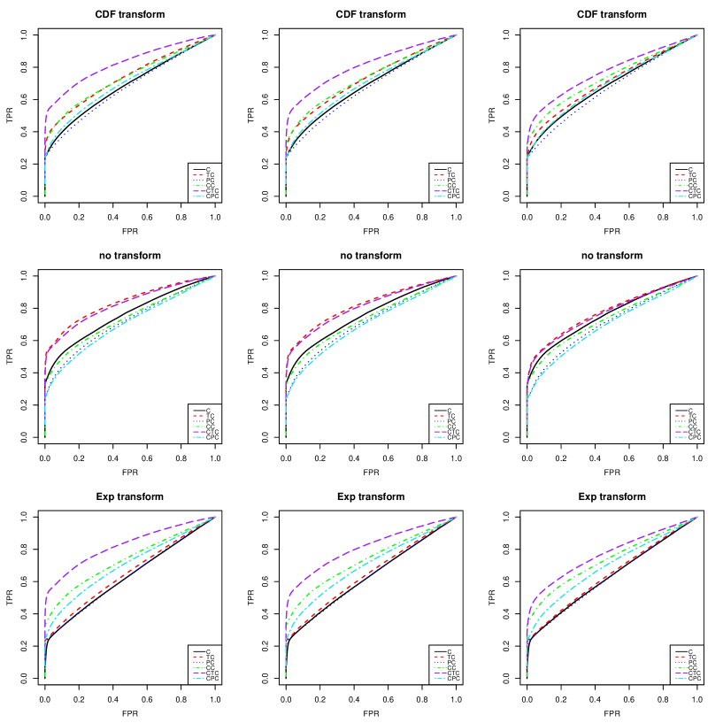
Figure 1: ROC curves for the Gaussian CDF, linear and exponential transformations (top, middle, bottom) using the six methods with banded graph structure, with similarity between the target study and auxiliary studies at different levels ($r=10,20,30$ from left to right), and $p=100,n=n_{1}=\dots=n_{k}=200,K=5,\mathcal{A}=\{1,2,3\}$.

5.2 Analysis of Simulation Results

5.2.1 Summary of the results

From the ROC curves in Figure 1 and Figure 2, we see that, if we have a certain number of informative auxiliary data, Trans-CLIME estimator performs slightly better than the Trans-Copula-CLIME estimator when the data is from Gaussian distribution. However, when the data is not from Gaussian distribution, the performance of the Trans-Copula-CLIME estimator is significantly better than the other five methods. This shows that the combination of transfer learning and semi-parametric method improves both statistical efficiency and estimation robustness. Likewise, the Copula CLIME estimator outperforms the CLIME estimator and the Copula Pooled Trans-CLIME estimator outperforms the Pooled Trans-CLIME estimator when the data are not from Gaussian, which shows the robustness of the semi-parametric methods once again.

In addition, we can also see that the performance of the Trans-Copula-CLIME estimator is the best among the three copula-based methods, followed by Copula CLIME, and the Copula Pooled Trans-CLIME performs the worst. Similarly, for the three parametric methods (CLIME, Trans-CLIME and Pooled Trans-CLIME), the performance of the Trans-CLIME estimator is better than CLIME estimator and the performance of the Pooled Trans-CLIME estimator is the worst. These results indicate that the informative auxiliary data can improve the performance of the estimator, while the non-informative auxiliary data makes no difference to the performance of the estimator. Instead, because we only use $2n/3$ samples to compute $\widehat{\Omega}^{(\text{CL})}$, the performance of the pooled version is even worse than CLIME or Copula CLIME estimator.

The performance of the Trans-Copula-CLIME estimator and Trans-CLIME estimator is related to the similarity between the target study and the auxiliary studies. When the similarity level increases, the performance of the two methods also improves. Especially when $r=10$ (the most similar case in our setting), which means the difference between the target study and the auxiliary studies is negligible, these two methods are far better than the corresponding CLIME method only using samples from the single target study.

From the estimation errors curves in terms of Frobenius norm shown in Figure 3 and Figure 4, we can draw similar conclusions. Besides, as the amount of informative auxiliary data increases, the estimation errors of the Trans-Copula-CLIME estimator and the Trans-CLIME estimator decrease, which validates our theoretical results. When the number of informative auxiliary studies is small, estimators based on pooled version do not work well. This is because $K-|\mathcal{A}|$ non-informative studies are used in the pooled version, which deteriorates the empirical performance. In the following, we make further analysis according to ROC curves in Figure 1 and Figure 2.

Figure 2: ROC curves for the Gaussian CDF, linear and exponential transformations (top, middle, bottom) using the six methods with block diagonal graph structure, with similarity between target study and auxiliary studies at different levels ($r=10,20,30$ from left to right), and $p=100,n=n_{1}=\dots=n_{k}=200,K=5,\mathcal{A}=\{1,2,3\}$.

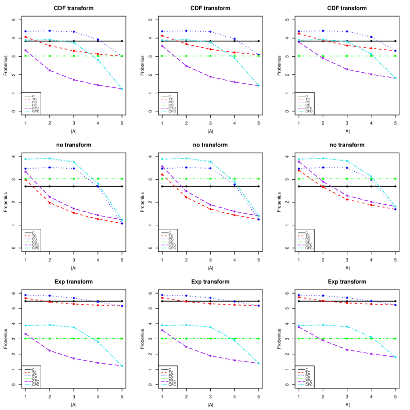
Figure 3: Estimation errors in Frobenius norm as a function of the number of informative studies for the Gaussian CDF, linear and exponential transformations (top, middle, bottom) using the six methods with banded graph structure, with similarity between target study and auxiliary studies at different levels ($r=10,20,30$ from left to right), and $p=100,n=n_{1}=\dots=n_{k}=200,K=5$.

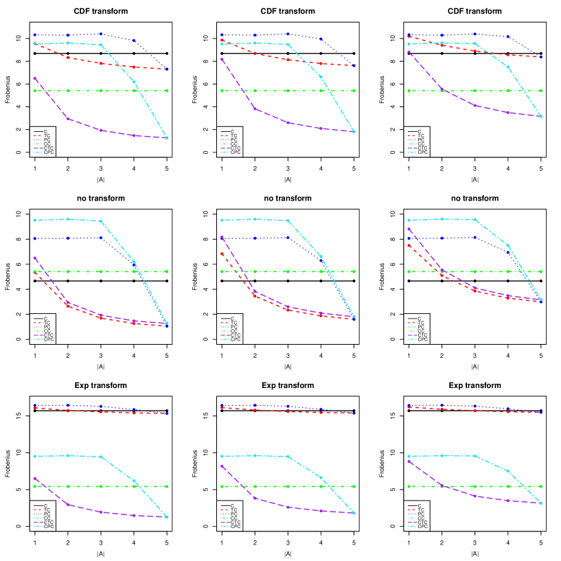
Figure 4: Estimation errors in Frobenius norm as a function of the number of informative studies for the Gaussian CDF, linear and exponential transformations (top, middle, bottom) using the six methods with block diagonal graph structure, with similarity between target study and auxiliary studies at different levels ($r=10,20,30$ from left to right), and $p=100,n=n_{1}=\dots=n_{k}=200,K=5$.

5.2.2 Non-Gaussian data

To compare the graph estimation performance of two procedures $A$ and $B$, in the following we use $A>B$ to represent that $A$ is better than $B$; $A\gg B$ means that $A$ is significantly better than $B$; $A\approx B$ means that $A$ and $B$ have similar performance.

The results of the comparison of the six methods with different precision matrices and transformation functions are as follows:
$\bullet$ Non-Gaussian data with banded matrix and CDF transformation: CTC$\gg$CC$>$TC$>$CPC$>$C$>$PC.
$\bullet$ Non-Gaussian data with banded matrix and Exp transformation: CTC$\gg$CC$>$CPC$>$TC$>$C$\approx$PC.
$\bullet$ Non-Gaussian data with block diagonal matrix and CDF transformation: CTC$>$TC$\gg$CC$\approx$C$>$CPC$\approx$PC.
$\bullet$ Non-Gaussian data with block diagonal matrix and Exp transformation: CTC$\gg$CC$>$CPC$>$TC$>$PC$>$C.

From the Gaussian CDF transformation and exponential transformation ROC curves in Figure 1 and Figure 2, we see that, the three copula-based methods are better than the corresponding parametric methods on the whole. The performance of the Trans-Copula-CLIME estimator is the best among the six methods and significantly better than Trans-CLIME estimator. Even the performance of the Copula CLIME estimator is better than Trans-CLIME estimator in some settings. Especially when the transformation function is exponential, the Copula Pooled Trans-CLIME estimator also outperforms Trans-CLIME estimator. This shows that the distribution of the data is very important for the choice of different methods. When the data comes from a non-Gaussian distribution, it is better to use semi-parametric approach with the single target study than to use parametric method with informative auxiliary data.

5.2.3 Gaussian data

The results of the comparison of the six methods with different precision matrices are as follows:
$\bullet$ Gaussian data with banded matrix: TC$>$CTC$\gg$C$>$CC$>$PC$>$CPC.
$\bullet$ Gaussian data block diagonal matrix: CTC$\approx$TC$\gg$C$>$CC$\approx$PC$>$CPC.

From linear transformation curves in Figure 1 and Figure 2, we see that, contrary to the results for non-Gaussian data, the performance of the Trans-CLIME estimator is slightly better than the Trans-Copula-CLIME estimator. The performance of the CLIME estimator is better than Copula CLIME estimator. The Pooled Trans-CLIME estimator outperforms Copula Pooled Trans-CLIME estimator. However, the ROC curves of Trans-CLIME estimator and Trans-Copula-CLIME estimator are pretty close. Especially when the precision matrix has block diagonal structure, Trans-CLIME estimator and Trans-Copula-CLIME estimator have similar performance, which shows the former does not show much advantage.

In summary, the simulation results show when the data does not satisfy the Gaussian assumption, the Trans-Copula-CLIME estimator still retains advantageous and is the best one among the six methods. This suggests that Trans-Copula-CLIME has higher statistical efficiency and shows estimation robustness in a wider range of applications. The higher the similarity level between the auxiliary studies and the target study, the more auxiliary samples, the better the estimator with transfer learning performs. However, the pooled versions are the worst among the six methods, indicating that when the auxiliary studies differs greatly from the target study, transfer learning does not work well. In practice, if we have informative auxiliary data, we can choose the more robust Trans-copula-CLIME to estimate the graph.

6 Real fMRI data related to ADHD

In this section, we apply the proposed algorithm to study the brain connectivity in patients with attention deficit hyperactivity disorder (ADHD) using the dataset from ADHD-200 Global Competition. The dataset includes demographical information and resting state functional magnetic resonance imaging (fMRI) of nearly one thousand children and adolescents, including both combined types of ADHD and typically developing controls (TDC). We focus our analysis on the fMRI data from Beijing and New York sites, with Beijing site dataset selected as the target study and the New York site data viewed as the auxiliary study. We preprocessed the dataset with steps including correction, smoothing, denoising, quality control and deletion of missing values, finally resulting in a dataset consisted of 74 combined ADHD subjects and 109 TDC subjects in Beijing site and 96 combined ADHD subjects and 91 TDC subjects in New York site. Each brain image was parcellated into 116 regions of interest (ROI) using the Anatomical Automatic Labeling (AAL) atlas. The time series of voxels within the same ROI were then averaged.

First, we use Henze-Zirkler’s multivariate normality test and Royston’s multivariate normality test in R package “MVN” (Korkmaz et al. (2014)) to check the normality of data and reject the null hypothesis (both $p$-values is zero or almost zero). Then, we use shapiro-Wilk test to check the normality of each dimension, and select some dimensions to draw the Q-Q plots, as shown in Figure 5. The top panel shows the Q-Q plots of ADHD subjects in Beijing site, and the bottom panel shows the Q-Q plots of TDC subjects in Beijing site. As can be seen from Figure 5, our data seriously violates the normality assumption. Hence, it is reasonable to use Trans-Copula-CLIME to analyze the data in the following.

Figure 5: Q-Q plots of ADHD subjects in Beijing (the first line) and TDC subjects in Beijing (the second line). ”d” stands for dimension, for example, ”d69” stands for 69th dimension.

We apply Trans-Copula-CLIME to estimate the brain connectivity of ADHD subjects from Beijing and use ADHD subjects from New York as the auxiliary study. Similarly, we apply Trans-Copula-CLIME to estimate the brain connectivity of TDC subjects from Beijing and use TDC subjects from New York as the auxiliary study. Then we identify ten brain regions with the greatest differences between the two estimated graphical models and draw Figure 6 using the BrainNet Viewer software (Xia et al. (2013)). In Figure 6, (a)-(c) show the connections between the ten brain regions and other brain regions in the graphical model of ADHD subjects from the axial view, coronal view, and sagittal view, respectively; (d)-(f) show the connections between these ten brain regions and other brain regions in the graphical model of TDC subjects from the axial view, coronal view, and sagittal view, respectively, (g)-(i) show the top 10% differential edges between the two graphical models between these ten brain regions and other brain regions from the axial view, coronal view, and sagittal view, respectively.

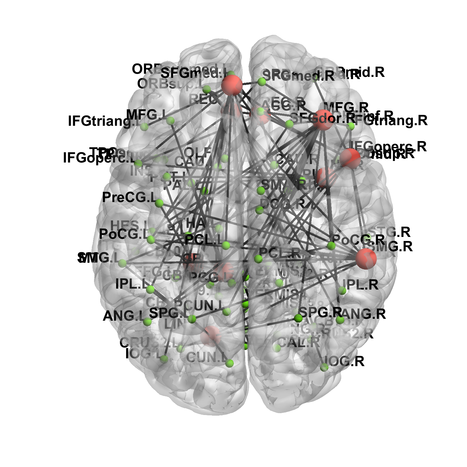
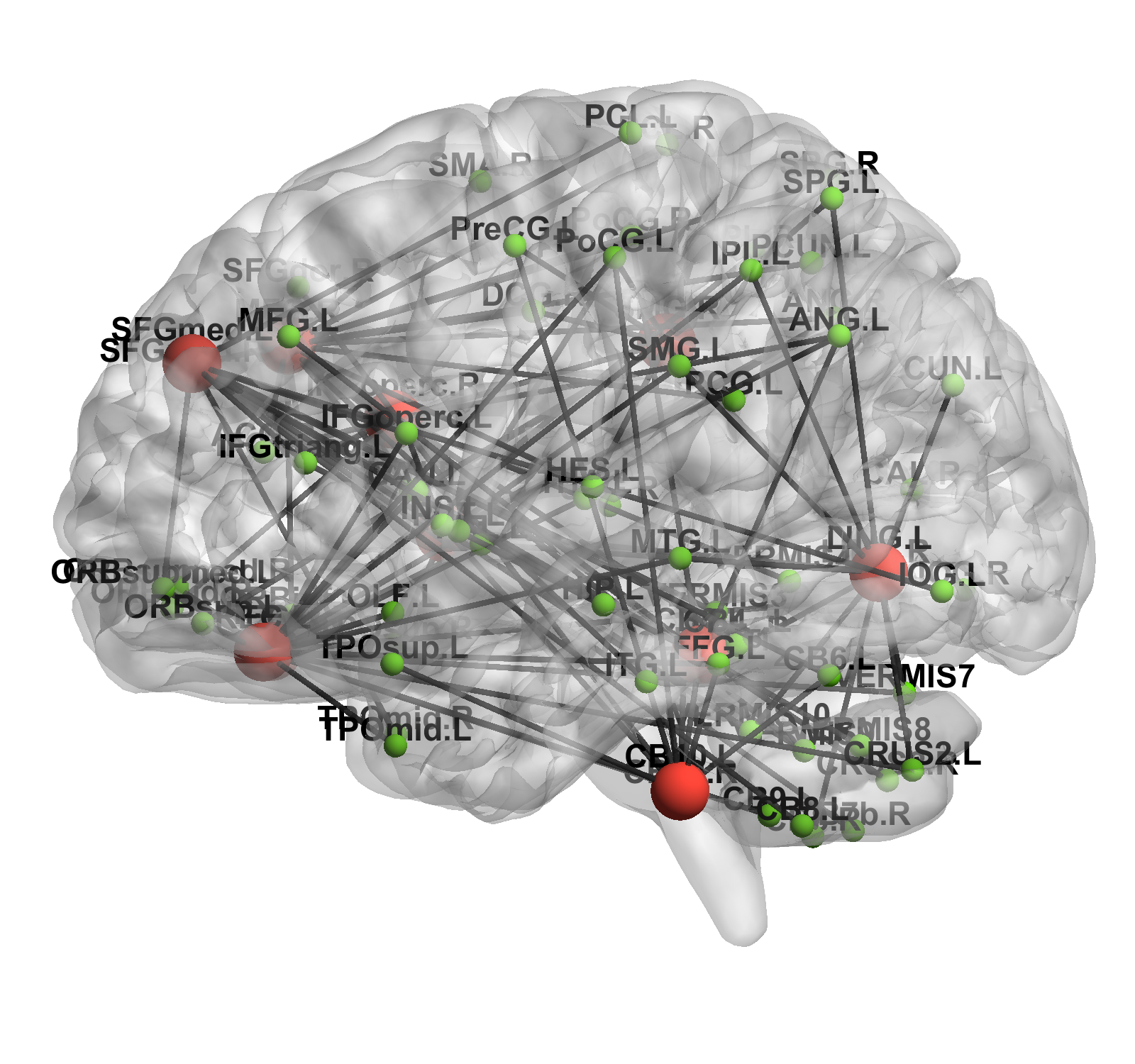
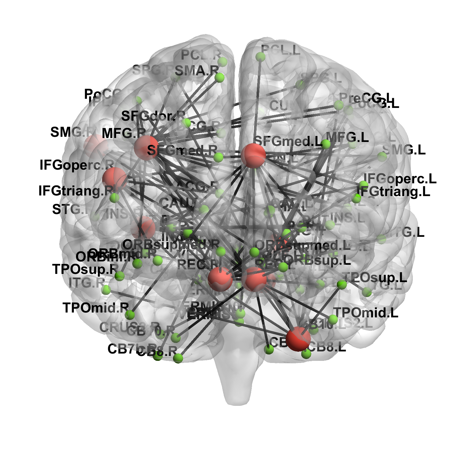
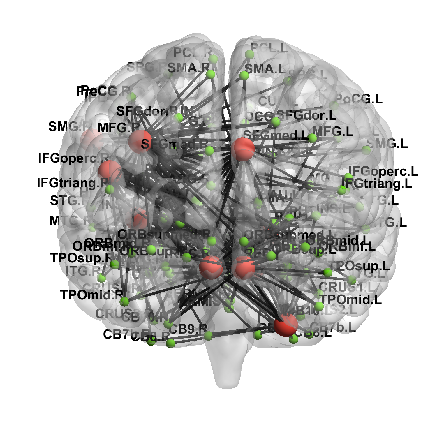
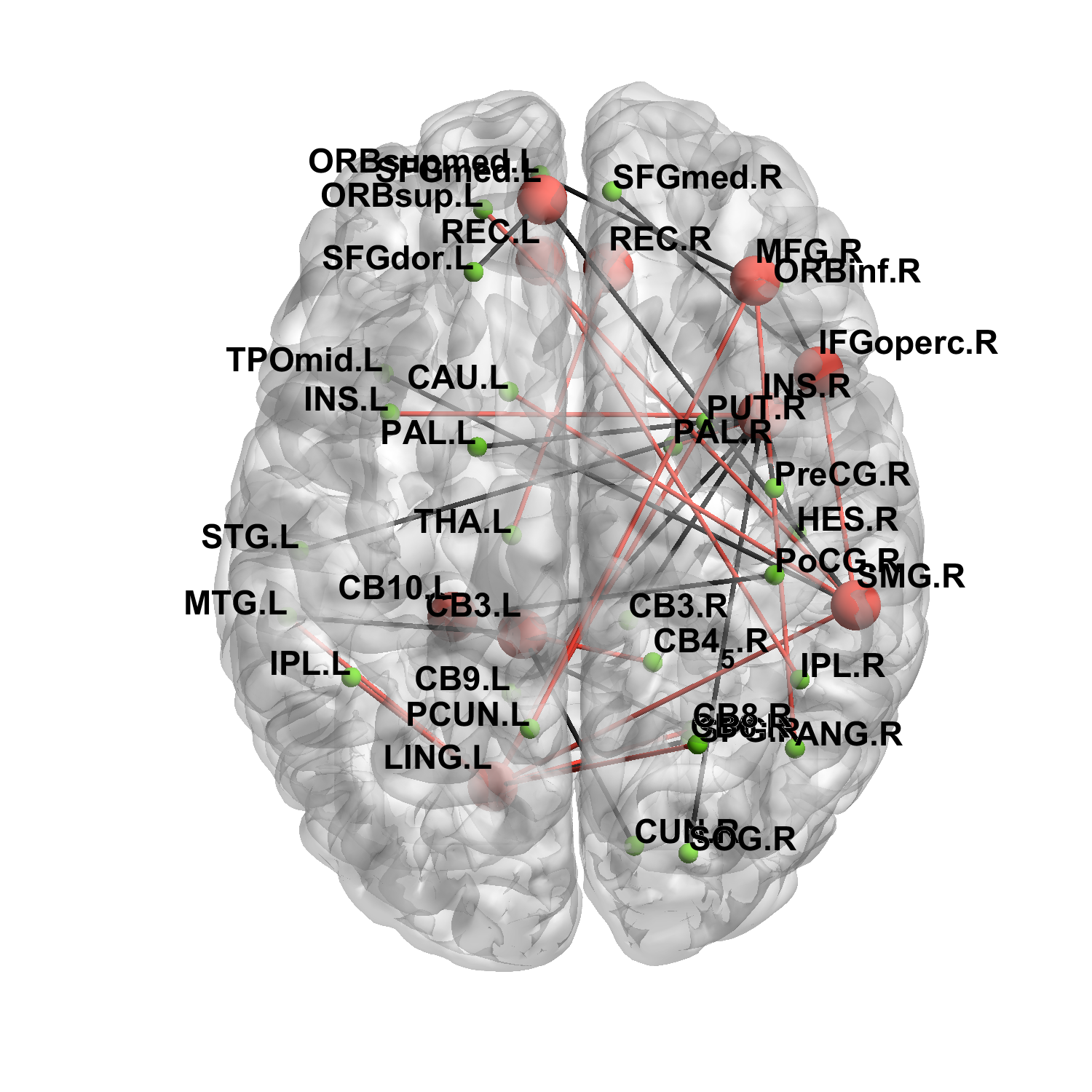
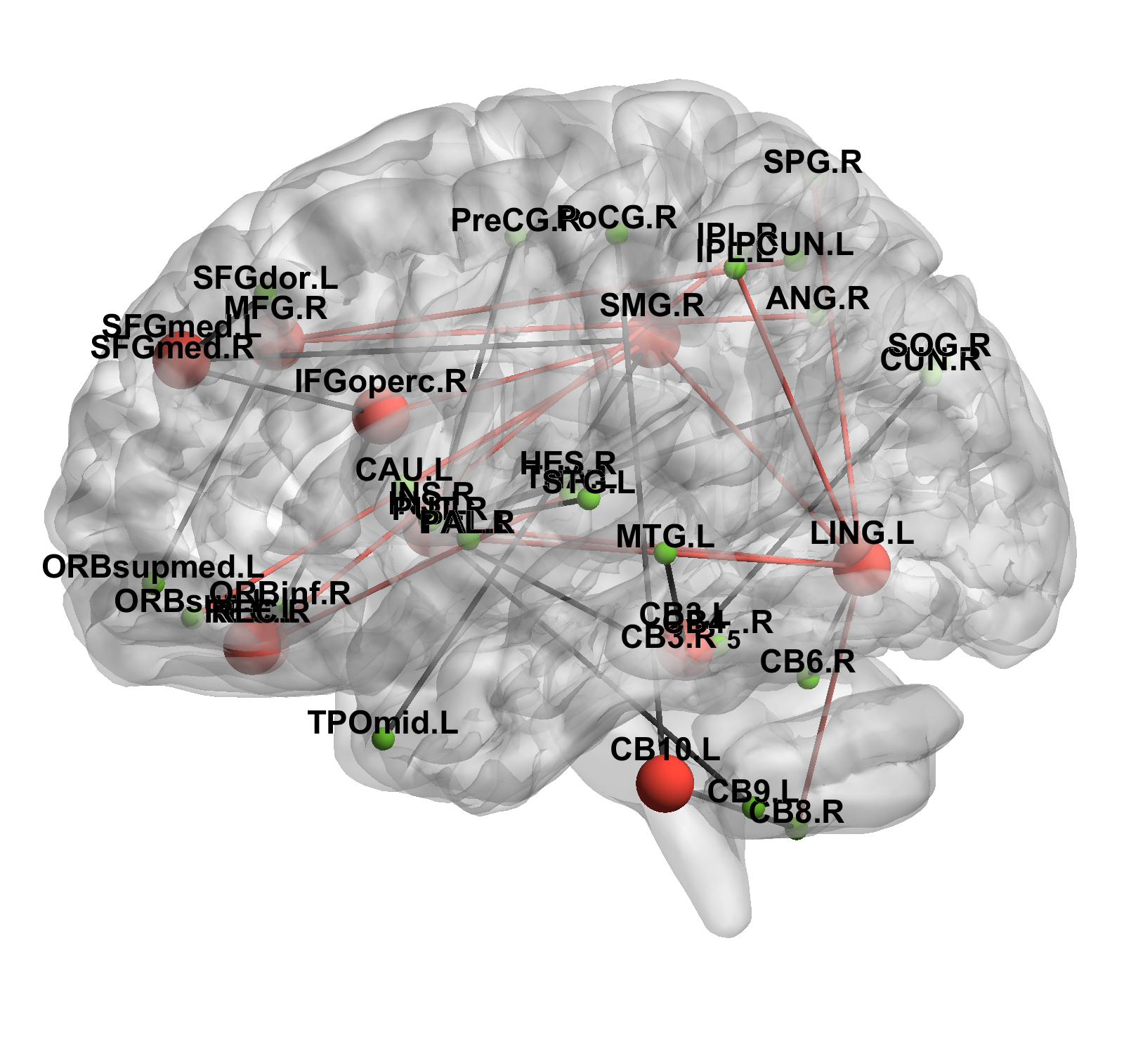
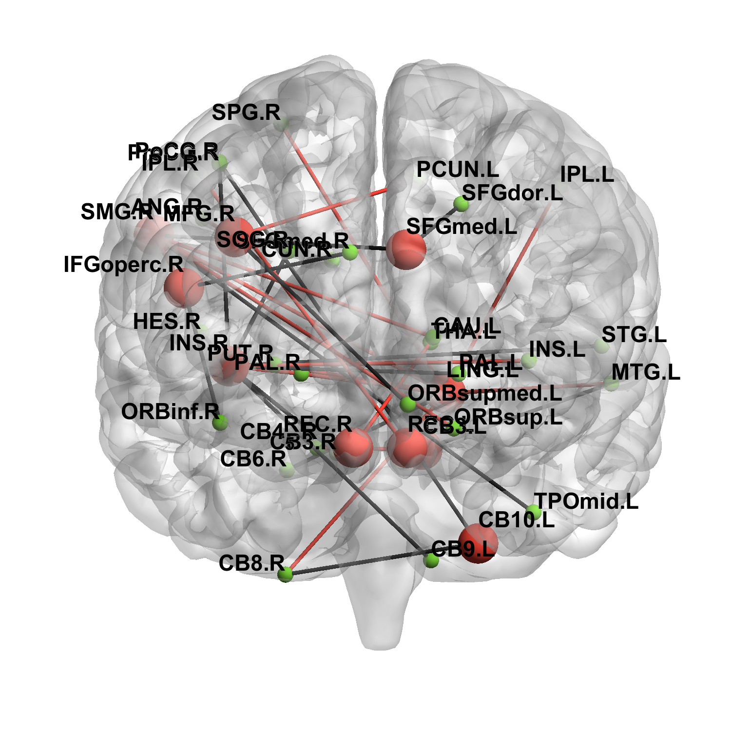
Figure 6: Graphical models estimated by Trans-Copula-CLIME for the ADHD resting-state fMRI data. (a)-(c) show the connections between the ten brain regions and other brain regions of ADHD subjects, (d)-(f) show the connections between these ten brain regions and other brain regions of TDC subjects, and (g)-(i) show the top 10% differential edges between the two graphical models. The red dots in (a)-(i) represent the ten brain regions with the greatest differences between the two graphical models, while the green dots represent the other brain regions. The red edges in (g)-(i) exist in the graph of ADHD subjects, but does not exist in the graph of TDC subjects; the black edges exist in the graph of TDC subjects, but does not exist in the graph of ADHD subjects.

As shown in Figure 6, the brain regions related to ADHD are mainly located in middle frontal gyrus, gyrus rectus, insula, supramarginal gyrus, inferior frontal gyrus opercular part, lingual gyrus, cerebellum and superior frontal gyrus medial. Many developmental disorders, such as ADHD and autism, are associated with cerebellar dysfunction, which may have long-term effects on motor, cognitive and emotional regulation (Stoodley, 2016). Ivanov et al. (2014) revealed that compared with the control group, adolescents with ADHD had smaller volumes in subregions of the cerebellum. It is reported that the middle frontal gyrus is involved in the storage and processing of working memory (Leung et al., 2002), and the lateral prefrontal cortex composed of the middle frontal gyrus is involved in dynamic cognitive control processes (Ridderinkhof et al., 2004). Ding and Pang (2021) found that the functional connectivity between the cerebellum and middle frontal gyrus was enhanced in ADHD children, which may lead to the disorder of the connection network, resulting in attention deficit in ADHD children. It was found that the right inferior frontal gyrus plays an important role in response inhibition and attentional control (Hampshire et al., 2010). Cubillo et al. (2010) revealed that patients with ADHD show fewer functional connectivity between the left and right inferior frontal gyrus, caudate/ thalamus, cingulate gyrus, and temporal/parietal regions during a response inhibition task than that in controls. Depue et al. (2010) found that there are morphological differences in inferior prefrontal regions between young people with ADHD and healthy controls. Patients with ADHD had smaller gray matter volume in the right inferior frontal gyrus, and this was associated with poorer behavioral performance. The insula plays a complex and critical role in human cognition, involving attention, emotional awareness, decision-making and cognitive control (Craig, 2009). Lopez-Larson et al. (2012) showed that the anterior insula gray matter volume of adolescents with ADHD was smaller than that of the healthy group. They further found that the left anterior insula gray matter was associated with oppositional symptoms, while the right anterior insula gray matter was associated with attention problems and inhibition. The lingual gyrus is involved in visual speech processing and word processing (Bogousslavsky et al., 1987; Mechelli et al., 2000). Ko et al. (2018) found that adults with ADHD responded to the dual-task effect with higher levels of activation in the left tongue region. Dibbets et al. (2010) found that ADHD patients have different activation patterns in brain frontal striatum circuit during the performance of an executive control task compared to the control group. Adults with ADHD showed greater activity in several brain regions such as the middle temporal gyrus, lingual gyrus and insula during task switching compared to healthy controls.

7 Conclusion

We proposed Trans-Copula-CLIME estimator to estimate an undirected graphical model by transfer learning information from auxiliary studies without Gaussian assumption. We obtain the asymptotic properties of the estimator in high-dimensional setting, which show that as long as we have sufficient samples from related auxiliary studies similar to target study, the transfer learning brings great advantage. Simulation studies validate the theoretical results and also show that Trans-Copula-CLIME estimator has better performance especially when data are not from Gaussian distribution. However, the theoretical properties of the estimator after aggregation step is still not clear, which is listed as our future research direction.

APPENDIX: PROOFS OF MAIN THEOREM

Appendix A Proofs of Main Theorems

To prove Theorem 4.1, we first present some useful lemmas. Lemma A.1 is adapted from Theorem 4.2 in Liu et al. (2012). Lemma A.2 establishes the convergence rate of $\widehat{S}^{\mathcal{A}}$ in element-wise matrix infinity norm. Lemma A.3 and Lemma A.4 provide two critical results in the proof of Theorem 4.1. Lemma A.5 establishes the convergence rate of each column of the CLIME estimator in terms of $\ell_{1}$ and $\ell_{2}$ norms.

A.1 Some useful lemmas

Lemma A.1.

(Convergence rate of $\widehat{S}$). For any $n>1$, we have

$$\mathbb{P}\bigg{(}\|\widehat{S}-\Sigma\|_{\max}\geqslant c_{1}\sqrt{\frac{\log p}{n}}\bigg{)}\leqslant\exp(-c_{2}\log p)$$

Lemma A.2.

(Convergence rate of $\widehat{S}^{\mathcal{A}}$)

$$\mathbb{P}\bigg{(}\|\widehat{S}^{\mathcal{A}}-\Sigma^{\mathcal{A}}\|_{\max}\geqslant c_{1}\sqrt{\frac{\log p}{n_{\mathcal{A}}}}\bigg{)}\leqslant\exp(-c_{2}\log p)$$

Lemma A.3.

For $\Sigma$ and its estimate $\widehat{S}$, if $\|\Sigma-\widehat{S}\|_{\infty,\infty}\leqslant\widetilde{\lambda}$, then $\forall u\in\mathcal{C}(S,\alpha)$, we have

$$u^{\top}\widehat{S}u\geqslant u^{\top}\Sigma u-\widetilde{\lambda}s(1+\alpha)^{2}\|u\|_{2}^{2}$$

where $\mathcal{C}(S,\alpha):=\{u\in\mathbb{R}^{p}|\ \|u_{S^{c}}\|_{1}\leqslant\alpha\|u_{S}\|_{1}\}$ and here $S$ is a support set with cardinality at most $s$.

Lemma A.4.

Under the conditions of Theorem 2.1, when $h\lesssim s\sqrt{\log p/n}$ and $n_{\mathcal{A}}\gtrsim n$, we have

$$\mathbb{P}\bigg{(}\max_{j}\|r_{j}(\widehat{\Delta}^{\mathcal{A}})-r_{j}(\Delta^{\mathcal{A}})\|_{2}^{2}\geqslant c_{1}h\delta_{n}\bigg{)}\leqslant\exp(-c_{2}\log p)+\exp(-c_{3}n)$$

for some positive constants $c_{1},c_{2}$ and $c_{3}$.

Lemma A.5.

(Convergence rate of CLIME). Under the conditions of Theorem 4.1, we have

$$\mathbb{P}\bigg{(}\|\widehat{\Omega}_{j}^{(\text{CL})}-\Omega_{j}\|_{1}\geqslant c_{1}s\sqrt{\frac{\log p}{n}}\bigg{)}\leqslant\exp(-c_{2}\log p)$$

$$\mathbb{P}\bigg{(}\|\widehat{\Omega}_{j}^{(\text{CL})}-\Omega_{j}\|_{2}^{2}\geqslant c_{1}s\frac{\log p}{n}\bigg{)}\leqslant\exp(-c_{2}\log p)$$

for some positive constants $c_{1},c_{2}$ and $c_{3}$.

A.2 Proof of Theorem 4.1

Proof.

The main idea of the proof are similar to lemma A.2 in Li et al. (2020), but there are some changes to the notation and proof details. We first establish the convergence rate of $\widehat{\Omega}^{L}$, where $\widehat{\Omega}^{L}$ is an estimate of $\Omega$ using method based on Lasso. Then we establish the convergence rate of $\widehat{\Omega}$ based on $\widehat{\Omega}^{L}$.

By Lemma 1 in Cai et al. (2011), problem (3.6) can be further casted as $p$ separate minimization problems and for $1\leqslant j\leqslant p$,

$$\widehat{\Omega}_{j}=\underset{\omega}{\arg\min}\|\omega\|_{1}$$ (A.1)

$$\quad\text{ subject to }\|\widehat{S}^{\mathcal{A}}\omega-(e_{j}+r_{j}(\widehat{\Delta}^{\mathcal{A}}))\|_{\infty}\leqslant\lambda_{\Omega}.$$

We consider the Lasso version for the $j$-th column

$$\widehat{\Omega}_{j}^{L}=\underset{\omega}{\arg\min}\frac{1}{2}\omega^{\top}\widehat{S}^{A}\omega-\omega^{\top}(e_{j}+r_{j}(\widehat{\Delta}^{\mathcal{A}}))+\lambda_{\Omega}\|\omega\|_{1}.$$ (A.2)

According to the above formula, we have oracle inequality:

$$\frac{1}{2} (\widehat{\Omega}_{j}^{L})^{\top}\widehat{S}^{A}\widehat{\Omega}_{j}^{L}-(\widehat{\Omega}_{j}^{L})^{\top}(e_{j}+r_{j}(\widehat{\Delta}^{\mathcal{A}}))+\lambda_{\Omega}\|\widehat{\Omega}_{j}^{L}\|_{1}$$ (A.3)

$$\leqslant\frac{1}{2}(\Omega_{j})^{\top}\widehat{S}^{\mathcal{A}}\Omega_{j}-\Omega_{j}^{\top}(e_{j}+r_{j}(\widehat{\Delta}^{\mathcal{A}}))+\lambda_{\Omega}\|\Omega_{j}\|_{1}.$$

Let $\Omega^{*}=\Omega+\Omega^{\mathcal{A}}(\widehat{\Delta}^{\mathcal{A}}-\Delta^{\mathcal{A}})^{\top}$. We view $\Omega^{*}_{j}$ as the true parameter and view $\Omega_{j}$ as a spare approximation of $\Omega^{*}_{j}$ in the following proof. With $\Omega^{*}_{j}$, the oracle inequality (A.3) can be transformed into the following form step by step:

$$\frac{1}{2}(\widehat{\Omega}_{j}^{L})^{\top}\widehat{S}^{\mathcal{A}}\widehat{\Omega}_{j}^{L}+\frac{1}{2}(\widehat{\Omega}_{j}^{*})^{\top}\widehat{S}^{\mathcal{A}}\widehat{\Omega}_{j}^{*}-(\Omega_{j}^{*})^{\top}\widehat{S}^{\mathcal{A}}\widehat{\Omega}_{j}^{L}-(\widehat{\Omega}_{j}^{L})^{\top}(e_{j}+r_{j}(\widehat{\Delta}^{\mathcal{A}}))+\lambda_{\Omega}\|\widehat{\Omega}_{j}^{L}\|_{1}$$

$$\text{\quad}\leqslant\frac{1}{2}\Omega_{j}^{\top}\widehat{S}^{\mathcal{A}}\Omega_{j}+\frac{1}{2}(\widehat{\Omega}_{j}^{*})^{\top}\widehat{S}^{\mathcal{A}}\widehat{\Omega}_{j}^{*}-(\Omega_{j}^{*})^{\top}\widehat{S}^{\mathcal{A}}\Omega_{j}+(\Omega_{j}^{*})^{\top}\widehat{S}^{\mathcal{A}}\Omega_{j}$$

$$\text{\qquad}-(\Omega_{j}^{*})^{\top}\widehat{S}^{\mathcal{A}}\widehat{\Omega}_{j}^{L}-\Omega_{j}^{\top}(e_{j}+r_{j}(\widehat{\Delta}^{\mathcal{A}}))+\lambda_{\Omega}\|\Omega_{j}\|_{1}$$

$$\Longrightarrow \frac{1}{2}(\widehat{\Omega}_{j}^{L}-\Omega_{j}^{*})^{\top}\widehat{S}^{\mathcal{A}}(\widehat{\Omega}_{j}^{L}-\Omega_{j}^{*})\leqslant\frac{1}{2}(\Omega_{j}-\Omega_{j}^{*})^{\top}\widehat{S}^{\mathcal{A}}(\Omega_{j}-\Omega_{j}^{*})$$

$$\text{\quad}+(\Omega_{j}-\widehat{\Omega}_{j}^{L})^{\top}(\widehat{S}^{\mathcal{A}}\Omega_{j}^{*}-(e_{j}+r_{j}(\widehat{\Delta}^{\mathcal{A}})))+\lambda_{\Omega}\|\Omega_{j}\|_{1}-\lambda_{\Omega}\|\widehat{\Omega}_{j}^{L}\|_{1}$$

$$\Longrightarrow \frac{1}{2}(\widehat{\Omega}_{j}^{L}-\Omega_{j}^{*})^{\top}\widehat{S}^{\mathcal{A}}(\widehat{\Omega}_{j}^{L}-\Omega_{j}^{*})\leqslant\frac{1}{2}(\Omega_{j}-\Omega_{j}^{*})^{\top}\widehat{S}^{\mathcal{A}}(\Omega_{j}-\Omega_{j}^{*})$$

$$\text{\quad}+|(\widehat{\Omega}_{j}^{L}-\Omega_{j})^{\top}(\widehat{S}^{\mathcal{A}}\Omega_{j}^{*}-(e_{j}+r_{j}(\widehat{\Delta}^{\mathcal{A}})))|+\lambda_{\Omega}\|\Omega_{j}\|_{1}-\lambda_{\Omega}\|\widehat{\Omega}_{j}^{L}\|_{1}.$$

Consider the event $\mathcal{E}_{1}=\big{\{}\|\widehat{S}^{\mathcal{A}}\Omega_{j}^{*}-(e_{j}-r_{j}(\widehat{\Delta}^{\mathcal{A}}))\|_{\infty}\leqslant\lambda_{\Omega}/2\big{\}}$. For this event, we have

$$\frac{1}{2}(\widehat{\Omega}_{j}^{L}-\Omega_{j}^{*})^{\top}\widehat{S}^{\mathcal{A}}(\widehat{\Omega}_{j}^{L}-\Omega_{j}^{*})\leqslant \frac{1}{2}(\Omega_{j}-\Omega_{j}^{*})^{\top}\widehat{S}^{\mathcal{A}}(\Omega_{j}-\Omega_{j}^{*})+\frac{\lambda_{\Omega}}{2}\|\widehat{\Omega}_{j}^{L}-\Omega_{j}\|_{1}+\lambda_{\Omega}\|\Omega_{j}\|_{1}-\lambda_{\Omega}\|\widehat{\Omega}_{j}^{L}\|_{1}$$

$$= \frac{1}{2}(\Omega_{j}-\Omega_{j}^{*})^{\top}\widehat{S}^{\mathcal{A}}(\Omega_{j}-\Omega_{j}^{*})+\frac{\lambda_{\Omega}}{2}\|\widehat{\Omega}_{S_{j},j}^{L}-\Omega_{S_{j},j}\|_{1}+\frac{\lambda_{\Omega}}{2}\|\widehat{\Omega}_{S_{j}^{c},j}^{L}\|_{1}$$

$$\text{\quad}+\lambda_{\Omega}\|\Omega_{S_{j},j}\|_{1}-\lambda_{\Omega}\|\widehat{\Omega}_{S_{j},j}^{L}\|_{1}-\lambda_{\Omega}\|\widehat{\Omega}_{S_{j}^{c},j}^{L}\|_{1}$$

$$\leqslant \frac{1}{2}(\Omega_{j}-\Omega_{j}^{*})^{\top}\widehat{S}^{\mathcal{A}}(\Omega_{j}-\Omega_{j}^{*})+\frac{3\lambda_{\Omega}}{2}\|\widehat{\Omega}_{S_{j},j}^{L}-\Omega_{S_{j},j}\|_{1}-\frac{\lambda_{\Omega}}{2}\|\widehat{\Omega}_{S_{j}^{c},j}^{L}-\Omega_{S_{j}^{c},j}\|_{1},$$

where we use the inequality $\|x\|_{1}-\|y\|_{1}\leqslant\|x-y\|_{1}$ for vectors $x$, $y$ in the last line. The left hand side can be lower bounded by

$$\frac{1}{4}(\widehat{\Omega}_{j}^{L}-\Omega_{j})^{\top}\widehat{S}^{\mathcal{A}}(\widehat{\Omega}_{j}^{L}-\Omega_{j})-\frac{1}{2}(\Omega_{j}-\Omega_{j}^{*})^{\top}\widehat{S}^{\mathcal{A}}(\Omega_{j}-\Omega_{j}^{*}).$$ (A.4)

Actually, due to positive semidefinite property of $\widehat{S}^{\mathcal{A}}$, we have

$$\text{\quad}\big{[}(\widehat{\Omega}_{j}^{L}-\Omega_{j}^{*})-(\Omega_{j}^{*}-\Omega_{j})\big{]}^{\top}\widehat{S}^{\mathcal{A}}\big{[}(\widehat{\Omega}_{j}^{L}-\Omega_{j}^{*})-(\Omega_{j}^{*}-\Omega_{j})\big{]}$$

$$=(\widehat{\Omega}_{j}^{L}-\Omega_{j}^{*})^{\top}\widehat{S}^{\mathcal{A}}(\widehat{\Omega}_{j}^{L}-\Omega_{j}^{*})+(\Omega_{j}^{*}-\Omega_{j})^{\top}\widehat{S}^{\mathcal{A}}(\Omega_{j}^{*}-\Omega_{j})-2(\widehat{\Omega}_{j}^{L}-\Omega_{j}^{*})^{\top}\widehat{S}^{\mathcal{A}}(\Omega_{j}^{*}-\Omega_{j})$$

$$\geqslant 0.$$

Hence, $2(\widehat{\Omega}_{j}^{L}-\Omega_{j}^{*})^{\top}\widehat{S}^{\mathcal{A}}(\Omega_{j}^{*}-\Omega_{j})\leqslant(\widehat{\Omega}_{j}^{L}-\Omega_{j}^{*})^{\top}\widehat{S}^{\mathcal{A}}(\widehat{\Omega}_{j}^{L}-\Omega_{j}^{*})+(\Omega_{j}^{*}-\Omega_{j})^{\top}\widehat{S}^{\mathcal{A}}(\Omega_{j}^{*}-\Omega_{j})$. Remark that if $\widehat{S}^{\mathcal{A}}$ is not positive semidefinite, we could make a projection of it into the space of semipositive definite matrices. On the other hand,

$$\text{\quad}(\widehat{\Omega}_{j}^{L}-\Omega_{j})^{\top}\widehat{S}^{\mathcal{A}}(\widehat{\Omega}_{j}^{L}-\Omega_{j})$$

$$=\big{[}(\widehat{\Omega}_{j}^{L}-\Omega_{j}^{*})+(\Omega_{j}^{*}-\Omega_{j})\big{]}^{\top}\widehat{S}^{\mathcal{A}}\big{[}(\widehat{\Omega}_{j}^{L}-\Omega_{j}^{*})+(\Omega_{j}^{*}-\Omega_{j})\big{]}$$

$$=(\widehat{\Omega}_{j}^{L}-\Omega_{j}^{*})^{\top}\widehat{S}^{\mathcal{A}}(\widehat{\Omega}_{j}^{L}-\Omega_{j}^{*})+(\Omega_{j}^{*}-\Omega_{j})^{\top}\widehat{S}^{\mathcal{A}}(\Omega_{j}^{*}-\Omega_{j})+2(\widehat{\Omega}_{j}^{L}-\Omega_{j}^{*})^{\top}\widehat{S}^{\mathcal{A}}(\Omega_{j}^{*}-\Omega_{j})$$

$$\leqslant 2(\widehat{\Omega}_{j}^{L}-\Omega_{j}^{*})^{\top}\widehat{S}^{\mathcal{A}}(\widehat{\Omega}_{j}^{L}-\Omega_{j}^{*})+2(\Omega_{j}^{*}-\Omega_{j})^{\top}\widehat{S}^{\mathcal{A}}(\Omega_{j}^{*}-\Omega_{j}),$$

which concludes (A.4). As a result,

$$\frac{1}{4}(\widehat{\Omega}_{j}^{L}-\Omega_{j})^{\top}\widehat{S}^{\mathcal{A}}(\widehat{\Omega}_{j}^{L}-\Omega_{j})\leqslant (\Omega_{j}-\Omega_{j}^{*})^{\top}\widehat{S}^{\mathcal{A}}(\Omega_{j}-\Omega_{j}^{*})$$ (A.5)

$$+\frac{3\lambda_{\Omega}}{2}\|\widehat{\Omega}_{S_{j},j}^{L}-\Omega_{S_{j},j}\|_{1}-\frac{\lambda_{\Omega}}{2}\|\widehat{\Omega}_{S_{j}^{c},j}^{L}-\Omega_{S_{j}^{c},j}\|_{1}.$$

Let’s consider the following two cases.
(i) If

$$\frac{3\lambda_{\Omega}}{2}\|\widehat{\Omega}_{S_{j},j}^{L}-\Omega_{S_{j},j}\|_{1}\geqslant(\Omega_{j}-\Omega_{j}^{*})^{\top}\widehat{S}^{\mathcal{A}}(\Omega_{j}-\Omega_{j}^{*}),$$

then inequality (A.5) can be further relaxed into the following two forms.

$$\frac{1}{4}(\widehat{\Omega}_{j}^{L}-\Omega_{j})^{\top}\widehat{S}^{\mathcal{A}}(\widehat{\Omega}_{j}^{L}-\Omega_{j})\leqslant 3\lambda_{\Omega}\|\widehat{\Omega}_{S_{j},j}^{L}-\Omega_{S_{j},j}\|_{1}-\frac{\lambda_{\Omega}}{2}\|\widehat{\Omega}_{S_{j}^{c},j}^{L}-\Omega_{S_{j}^{c},j}\|_{1}$$ (A.6)

$$\frac{1}{4}(\widehat{\Omega}_{j}^{L}-\Omega_{j})^{\top}\widehat{S}^{\mathcal{A}}(\widehat{\Omega}_{j}^{L}-\Omega_{j})\leqslant 3\lambda_{\Omega}\|\widehat{\Omega}_{S_{j},j}^{L}-\Omega_{S_{j},j}\|_{1}$$ (A.7)

Using (A.6) and taking advantage of $\widehat{S}^{\mathcal{A}}$’s positive semidefinite property, we have

$$\|\widehat{\Omega}_{S_{j}^{c},j}^{L}-\Omega_{S_{j}^{c},j}\|_{1}\leqslant 6\|\widehat{\Omega}_{S_{j},j}^{L}-\Omega_{S_{j},j}\|_{1}.$$

In the event $\mathcal{E}_{2}=\bigg{\{}\inf\limits_{\|u_{S_{j}^{c}}\|_{1}\leqslant 6\|u_{S_{j}}\|_{1}\neq 0}\frac{u^{\top}\widehat{S}^{\mathcal{A}}u}{\|u\|_{2}^{2}}\geqslant\phi_{0}>0\bigg{\}}$, we have

$$\phi_{0}\|\widehat{\Omega}_{j}^{L}-\Omega_{j}\|_{2}^{2}\leqslant(\widehat{\Omega}_{j}^{L}-\Omega_{j})^{\top}\widehat{S}^{\mathcal{A}}(\widehat{\Omega}_{j}^{L}-\Omega_{j}).$$

Combining (A.7), we obtain

$$\frac{\phi_{0}}{4}\|\widehat{\Omega}_{j}^{L}-\Omega_{j}\|_{2}^{2}\leqslant 3\lambda_{\Omega}\|\widehat{\Omega}_{S_{j},j}^{L}-\Omega_{S_{j},j}\|_{1}\leqslant 3\sqrt{s_{j}}\lambda_{\Omega}\|\widehat{\Omega}_{S_{j},j}^{L}-\Omega_{S_{j},j}\|_{2}\leqslant 3\sqrt{s_{j}}\lambda_{\Omega}\|\widehat{\Omega}_{j}^{L}-\Omega_{j}\|_{2},$$

which gives

$$\|\widehat{\Omega}_{j}^{L}-\Omega_{j}\|_{2}\leqslant 12\sqrt{s_{j}}\lambda_{\Omega}/\phi_{0}.$$

(ii) If

$$\frac{3\lambda_{\Omega}}{2}\|\widehat{\Omega}_{S_{j},j}^{L}-\Omega_{S_{j},j}\|_{1}\leqslant(\Omega_{j}-\Omega_{j}^{*})^{\top}\widehat{S}^{\mathcal{A}}(\Omega_{j}-\Omega_{j}^{*}),$$ (A.8)

then inequality (A.5) also can be further relaxed into the following two forms.

$$\frac{1}{4}(\widehat{\Omega}_{j}^{L}-\Omega_{j})^{\top}\widehat{S}^{\mathcal{A}}(\widehat{\Omega}_{j}^{L}-\Omega_{j})\leqslant 2(\Omega_{j}-\Omega_{j}^{*})^{\top}\widehat{S}^{\mathcal{A}}(\Omega_{j}-\Omega_{j}^{*})-\frac{\lambda_{\Omega}}{2}\|\widehat{\Omega}_{S_{j}^{c}j}^{L}-\Omega_{S_{j}^{c},j}\|_{1}$$ (A.9)

$$\frac{1}{4}(\widehat{\Omega}_{j}^{L}-\Omega_{j})^{\top}\widehat{S}^{\mathcal{A}}(\widehat{\Omega}_{j}^{L}-\Omega_{j})\leqslant 2(\Omega_{j}-\Omega_{j}^{*})^{\top}\widehat{S}^{\mathcal{A}}(\Omega_{j}-\Omega_{j}^{*})$$ (A.10)

Again, using positive semidefinite property of $\widehat{S}^{\mathcal{A}}$ and (A.9), we have

$$\lambda_{\Omega}\|\widehat{\Omega}_{S_{j}^{c},j}^{L}-\Omega_{S_{j}^{c},j}\|_{1}\leqslant 4(\Omega_{j}-\Omega_{j}^{*})^{\top}\widehat{S}^{\mathcal{A}}(\Omega_{j}-\Omega_{j}^{*}).$$ (A.11)

Combining (A.8) and (A.11), we obtain

$$\lambda_{\Omega}\|\widehat{\Omega}_{j}^{L}-\Omega_{j}\|_{1}=\lambda_{\Omega}\|\widehat{\Omega}_{S_{j},j}^{L}-\Omega_{S_{j},j}\|_{1}+\lambda_{\Omega}\|\widehat{\Omega}_{S_{j}^{c},j}^{L}-\Omega_{S_{j}^{c},j}\|_{1}\leqslant\frac{14}{3}(\Omega_{j}-\Omega_{j}^{*})^{\top}\widehat{S}^{\mathcal{A}}(\Omega_{j}-\Omega_{j}^{*}).$$

Then we bound the term on the RHS

$$(\Omega_{j}-\Omega_{j}^{*})^{\top}\widehat{S}^{\mathcal{A}}(\Omega_{j}-\Omega_{j}^{*})=(r_{j}(\widehat{\Delta}^{\mathcal{A}}-\Delta^{\mathcal{A}}))^{\top}\Omega^{\mathcal{A}}\widehat{S}^{\mathcal{A}}\Omega^{\mathcal{A}}r_{j}(\widehat{\Delta}^{\mathcal{A}}-\Delta^{\mathcal{A}})$$

$$\leqslant(r_{j}(\widehat{\Delta}^{\mathcal{A}}-\Delta^{\mathcal{A}}))^{\top}\Omega^{\mathcal{A}}r_{j}(\widehat{\Delta}^{\mathcal{A}}-\Delta^{\mathcal{A}})+\|\Omega^{\mathcal{A}}(\widehat{S}^{\mathcal{A}}-\widehat{S}^{\mathcal{A}})\Omega^{\mathcal{A}}\|_{\infty,\infty}\|r_{j}(\widehat{\Delta}^{\mathcal{A}}-\Delta^{\mathcal{A}})\|_{1}^{2}$$

$$\leqslant ch\delta_{n}$$

with probability at least $1-\exp(c_{1}\log p)$. For any $\|u\|_{1}\leqslant\frac{14}{3}(\Omega_{j}-\Omega_{j}^{*})^{\top}\widehat{S}^{\mathcal{A}}(\Omega_{j}-\Omega_{j}^{*})/\lambda_{\Omega}$, it holds that

$$u^{\top}\widehat{S}^{\mathcal{A}}u\geqslant u^{\top}\Sigma^{\mathcal{A}}u-c_{1}\|\widehat{S}^{\mathcal{A}}-\Sigma^{\mathcal{A}}\|_{\max}\big{(}(\Omega_{j}-\Omega_{j}^{*})^{\top}\widehat{S}^{\mathcal{A}}(\Omega_{j}-\Omega_{j}^{*})\big{)}^{2}.$$

Therefore,

$$\Lambda_{\min}(\Sigma^{A})\|\widehat{\Omega}_{j}^{L}-\Omega_{j}\|_{2}^{2}\leqslant c(\Omega_{j}-\Omega_{j}^{*})^{\top}\widehat{S}^{\mathcal{A}}(\Omega_{j}-\Omega_{j}^{*})\leqslant ch\delta_{n}$$

provided that $h\delta_{n}/\lambda_{\Omega}=O(1)$. To summarize, in event $\mathcal{E}=\{\mathcal{E}_{1}\cap\mathcal{E}_{2}\}$, we have

$$\|\widehat{\Omega}_{j}^{L}-\Omega_{j}\|_{2}^{2}\leqslant c_{1}s\lambda_{\Omega}^{2}+c_{2}h\delta_{n}.$$

It remains to lower bound the probability of the event $\mathcal{E}=\{\mathcal{E}_{1}\cap\mathcal{E}_{2}\}$. We have the following decomposition.

$$\widehat{S}^{\mathcal{A}}\Omega_{j}^{*}-(e_{j}+r_{j}(\widehat{\Delta}^{\mathcal{A}}))=\widehat{S}^{\mathcal{A}}\Omega_{j}+\widehat{S}^{\mathcal{A}}\Omega^{\mathcal{A}}r_{j}(\widehat{\Delta}^{\mathcal{A}}-\Delta^{\mathcal{A}})-e_{j}-r_{j}(\widehat{\Delta}^{\mathcal{A}})$$

$$=\widehat{S}^{\mathcal{A}}\Omega_{j}+\widehat{S}^{\mathcal{A}}\Omega^{\mathcal{A}}r_{j}(\widehat{\Delta}^{\mathcal{A}}-\Delta^{\mathcal{A}})-e_{j}-r_{j}(\widehat{\Delta}^{\mathcal{A}})-r_{j}(\Delta^{\mathcal{A}})+r_{j}(\Delta^{\mathcal{A}})$$

$$=\widehat{S}^{\mathcal{A}}\Omega_{j}-e_{j}-r_{j}(\Delta^{\mathcal{A}})+(\widehat{S}^{\mathcal{A}}\Omega^{\mathcal{A}}-I_{p})r_{j}(\widehat{\Delta}^{\mathcal{A}}-\Delta^{\mathcal{A}})$$

$$=(\widehat{S}^{\mathcal{A}}-\Sigma^{\mathcal{A}})\Omega_{j}+(\widehat{S}^{\mathcal{A}}\Omega^{\mathcal{A}}-I_{p})r_{j}(\widehat{\Delta}^{\mathcal{A}}-\Delta^{\mathcal{A}})$$

Using $\|AB\|_{\max}\leqslant\|A\|_{\max}\|B\|_{1}$, we have

$$\|(\widehat{S}^{\mathcal{A}}-\Sigma^{\mathcal{A}})\Omega_{j}\|_{\max}\leqslant\|\widehat{S}^{\mathcal{A}}-\Sigma^{\mathcal{A}}\|_{\max}\|\Omega_{j}\|_{1}\leqslant c_{1}\sqrt{\frac{\log p}{n_{\mathcal{A}}}}$$

$$\|(\widehat{S}^{\mathcal{A}}\Omega^{\mathcal{A}}-I_{p})r_{j}(\widehat{\Delta}^{\mathcal{A}}-\Delta^{\mathcal{A}})\|_{\max}\leqslant\|\widehat{S}^{\mathcal{A}}\Omega^{\mathcal{A}}-I_{p}\|_{\max}\|r_{j}(\widehat{\Delta}^{\mathcal{A}}-\Delta^{\mathcal{A}})\|_{1}$$

$$\text{\qquad}\leqslant\|\widehat{S}^{\mathcal{A}}-\Sigma^{\mathcal{A}}\|_{\max}\|\Omega^{\mathcal{A}}\|_{1}\|r_{j}(\widehat{\Delta}^{\mathcal{A}}-\Delta^{\mathcal{A}})\|_{1}\leqslant c_{2}h\sqrt{\frac{\log p}{n_{\mathcal{A}}}}$$

for some constant $c_{1}$ and $c_{2}$ with probability at least $1-\exp(-c_{3}\log p)$. By $h\lesssim s\sqrt{\log p/n}\leqslant c$, it follows from the above results that

$$\|\widehat{S}^{\mathcal{A}}\Omega_{j}^{*}-(e_{j}+r_{j}(\widehat{\Delta}^{\mathcal{A}}))\|_{\max}\leqslant \|(\widehat{S}^{\mathcal{A}}-\Sigma^{\mathcal{A}})\Omega_{j}\|_{\max}+\|(\widehat{S}^{\mathcal{A}}\Omega^{\mathcal{A}}-I_{p})r_{j}(\widehat{\Delta}^{\mathcal{A}}-\Delta^{\mathcal{A}})\|_{\max}$$

$$\leqslant c_{4}\sqrt{\frac{\log p}{n_{\mathcal{A}}}}$$

with probability at least $1-\exp(-c_{3}\log p)$. Hence, $\mathbb{P}(\mathcal{E}_{1})\geqslant 1-\exp(-c_{3}\log p)$ for $\lambda_{\Omega}\geqslant 2c_{4}\sqrt{\frac{\log p}{n_{\mathcal{A}}}}$. Using lemma A.3, it is easy to show that $\mathbb{P}(\mathcal{E}_{2})\geqslant 1-\exp(-c_{1}\log p)$ provided that $s^{2}\log p=o(n_{\mathcal{A}})$. This completes the proof of the first result.

Then, we establish the convergence rate of $\widehat{\Omega}$ based on $\widehat{\Omega}^{L}$. According to (A.2), we have oracle inequality:

$$\frac{1}{2} (\widehat{\Omega}_{j}^{L})^{\top}\widehat{S}^{\mathcal{A}}\widehat{\Omega}_{j}^{L}-(\widehat{\Omega}_{j}^{L})^{\top}(e_{j}+r_{j}(\widehat{\Delta}^{\mathcal{A}}))+\lambda_{\Omega}\|\widehat{\Omega}_{j}^{L}\|_{1}$$

$$\leqslant\frac{1}{2}(\widehat{\Omega}_{j})^{\top}\widehat{S}^{\mathcal{A}}\widehat{\Omega}_{j}-\widehat{\Omega}_{j}^{\top}(e_{j}+r_{j}(\widehat{\Delta}^{\mathcal{A}}))+\lambda_{\Omega}\|\widehat{\Omega}_{j}\|_{1}.$$

As $\widehat{\Omega}_{j}^{L}$ is a feasible solution to (A.1), we have $\|\widehat{\Omega}_{j}\|_{1}\leqslant\|\widehat{\Omega}_{j}^{L}\|_{1}$. This leads to the following inequality

$$\frac{1}{2}(\widehat{\Omega}_{j}^{L})^{\top}\widehat{S}^{\mathcal{A}}\widehat{\Omega}_{j}^{L}-(\widehat{\Omega}_{j}^{L})^{\top}(e_{j}+r_{j}(\widehat{\Delta}^{\mathcal{A}}))\leqslant\frac{1}{2}\widehat{\Omega}_{j}^{\top}\widehat{S}^{\mathcal{A}}\widehat{\Omega}_{j}-\widehat{\Omega}_{j}^{\top}(e_{j}+r_{j}(\widehat{\Delta}^{\mathcal{A}})),$$

and it can be transformed into the following form

$$\frac{1}{2}(\widehat{\Omega}_{j}^{L})^{\top}\widehat{S}^{\mathcal{A}}\widehat{\Omega}_{j}^{L}+\frac{1}{2}\widehat{\Omega}_{j}^{\top}\widehat{S}^{\mathcal{A}}\widehat{\Omega}_{j}-\widehat{\Omega}_{j}^{\top}\widehat{S}^{\mathcal{A}}\widehat{\Omega}_{j}^{L}$$

$$\text{\quad}\leqslant\widehat{\Omega}_{j}^{\top}\widehat{S}^{\mathcal{A}}\widehat{\Omega}_{j}-\widehat{\Omega}_{j}^{\top}\widehat{S}^{\mathcal{A}}\widehat{\Omega}_{j}^{L}+(\widehat{\Omega}_{j}^{L}-\widehat{\Omega}_{j})^{\top}(e_{j}+r_{j}(\widehat{\Delta}^{\mathcal{A}}))$$

$$\Longrightarrow \frac{1}{2}(\widehat{\Omega}_{j}^{L}-\widehat{\Omega}_{j})^{\top}\widehat{S}^{\mathcal{A}}(\widehat{\Omega}_{j}^{L}-\widehat{\Omega}_{j})\leqslant(\widehat{\Omega}_{j}-\widehat{\Omega}_{j}^{L})^{\top}(\widehat{S}^{\mathcal{A}}\widehat{\Omega}_{j}-(e_{j}+r_{j}(\widehat{\Delta}^{\mathcal{A}})))$$

$$\Longrightarrow (\widehat{\Omega}_{j}-\widehat{\Omega}_{j}^{L})^{\top}\widehat{S}^{\mathcal{A}}(\widehat{\Omega}_{j}-\widehat{\Omega}_{j}^{L})\leqslant 2\lambda_{\Omega}\|\widehat{\Omega}_{j}-\widehat{\Omega}_{j}^{L}\|_{1}.$$ (A.12)

The inequality $\|\widehat{\Omega}_{j}\|_{1}\leqslant\|\widehat{\Omega}_{j}^{L}\|_{1}$ is equivalent to

$$\|\widehat{\Omega}_{S_{j},j}\|_{1}+\|\widehat{\Omega}_{S_{j}^{c},j}\|_{1}\leqslant\|\widehat{\Omega}_{S_{j},j}^{L}\|_{1}+\|\widehat{\Omega}_{S_{j}^{c},j}^{L}\|_{1}$$

and from that we can obtain

$$\|\widehat{\Omega}_{S_{j}^{c},j}-\widehat{\Omega}_{S_{j}^{c},j}^{L}\|_{1}\leqslant \|\widehat{\Omega}_{S_{j}^{c},j}\|_{1}+\|\widehat{\Omega}_{S_{j}^{c},j}^{L}\|_{1}\leqslant\|\widehat{\Omega}_{S_{j},j}^{L}\|_{1}-\|\widehat{\Omega}_{S_{j},j}\|_{1}+2\|\widehat{\Omega}_{S_{j}^{c},j}^{L}\|_{1}$$ (A.13)

$$\leqslant \|\widehat{\Omega}_{S_{j}}-\widehat{\Omega}_{S_{j},j}^{L}\|_{1}+2\|\widehat{\Omega}_{S_{j}^{c},j}^{L}\|_{1}$$

where we use the inequality $\|x\|_{1}-\|y\|_{1}\leqslant\|x-y\|_{1}$ again. Hence, we have

$$\|\widehat{\Omega}_{j}-\widehat{\Omega}_{j}^{L}\|_{1}= \|\widehat{\Omega}_{S_{j},j}-\widehat{\Omega}_{S_{j},j}^{L}\|_{1}+\|\widehat{\Omega}_{S_{j}^{c},j}-\widehat{\Omega}_{S_{j}^{c},j}^{L}\|_{1}$$

$$\leqslant 2\|\widehat{\Omega}_{S_{j},j}-\widehat{\Omega}_{S_{j},j}^{L}\|_{1}+2\|\widehat{\Omega}_{S_{j}^{c},j}^{L}\|_{1}$$

We can then separately discuss the two cases: $\|\widehat{\Omega}_{S_{j},j}-\widehat{\Omega}_{S_{j},j}^{L}\|_{1}\geqslant\|\widehat{\Omega}_{S_{j}^{c},j}^{L}\|_{1}$ and $\|\widehat{\Omega}_{S_{j},j}-\widehat{\Omega}_{S_{j},j}^{L}\|_{1}\leqslant\|\widehat{\Omega}_{S_{j},j}^{L}\|_{1}.$
(a)If

$$\|\widehat{\Omega}_{S_{j},j}-\widehat{\Omega}_{S_{j},j}^{L}\|_{1}\geqslant\|\widehat{\Omega}_{S_{j}^{c},j}^{L}\|_{1},$$

then according to (A.13), we have

$$\|\widehat{\Omega}_{S_{j}^{c},j}-\widehat{\Omega}_{S_{j}^{c},j}^{L}\|_{1}\leqslant 3\|\widehat{\Omega}_{S_{j},j}-\widehat{\Omega}_{S_{j},j}^{L}\|_{1}$$

and

$$\|\widehat{\Omega}_{j}-\widehat{\Omega}_{j}^{L}\|_{1}\leqslant 4\|\widehat{\Omega}_{S_{j},j}-\widehat{\Omega}_{S_{j},j}^{L}\|_{1}.$$

Using lemma A.3, we have

$$(\widehat{\Omega}_{j}-\widehat{\Omega}_{j}^{L})^{\top}\widehat{S}^{\mathcal{A}}(\widehat{\Omega}_{j}-\widehat{\Omega}_{j}^{L})\geqslant(\widehat{\Omega}_{j}-\widehat{\Omega}_{j}^{L})^{\top}\Sigma^{\mathcal{A}}(\widehat{\Omega}_{j}-\widehat{\Omega}_{j}^{L})-cs\sqrt{\frac{\log p}{n_{\mathcal{A}}}}\|\widehat{\Omega}_{j}-\widehat{\Omega}_{j}^{L}\|_{2}^{2}.$$

Invoking that under our assumptions, $s\sqrt{\frac{\log p}{n_{\mathcal{A}}}}=o(1)$, then

$$c\|\widehat{\Omega}_{j}-\widehat{\Omega}_{j}^{L}\|_{2}^{2}\leqslant(\widehat{\Omega}_{j}-\widehat{\Omega}_{j}^{L})^{\top}\widehat{S}^{\mathcal{A}}(\widehat{\Omega}_{j}-\widehat{\Omega}_{j}^{L}).$$

Combining (A.12), we have

$$c\|\widehat{\Omega}_{j}-\widehat{\Omega}_{j}^{L}\|_{2}^{2}\leqslant 8\lambda_{\Omega}\|\widehat{\Omega}_{S_{j},j}-\widehat{\Omega}_{S_{j},j}^{L}\|_{1}\leqslant 8\sqrt{s}\lambda_{\Omega}\|\widehat{\Omega}_{j}-\widehat{\Omega}_{j}^{L}\|_{2},$$

which gives

$$\|\widehat{\Omega}_{j}-\widehat{\Omega}_{j}^{L}\|_{2}^{2}\leqslant c_{1}s\lambda_{\Omega}^{2}.$$

(b)If

$$\|\widehat{\Omega}_{S_{j},j}-\widehat{\Omega}_{S_{j},j}^{L}\|_{1}\leqslant\|\widehat{\Omega}_{S_{j}^{c},j}^{L}\|_{1},$$

then according to (A.13), we have

$$\|\widehat{\Omega}_{S_{j}^{c},j}-\widehat{\Omega}_{S_{j}^{c},j}^{L}\|_{1}\leqslant 3\|\widehat{\Omega}_{S_{j}^{c},j}^{L}\|_{1}$$

and

$$\|\widehat{\Omega}_{j}-\widehat{\Omega}_{j}^{L}\|_{1}\leqslant 4\|\widehat{\Omega}_{S_{j}^{c},j}^{L}\|_{1}.$$

If case (i) discussed above, we have

$$\|\widehat{\Omega}_{S_{j}^{c},j}^{L}\|_{1}=\|\widehat{\Omega}_{S_{j}^{c},j}^{L}-\Omega_{S_{j}^{c},j}\|_{1}\leqslant 6\|\widehat{\Omega}_{S_{j},j}^{L}-\Omega_{S_{j},j}\|_{1}\leqslant c_{1}s\lambda_{\Omega}.$$

In case (ii) discussed above, we have

$$\lambda_{\Omega}\|\widehat{\Omega}_{S_{j}^{c},j}^{L}\|_{1}\leqslant 3(\Omega_{j}-\Omega_{j}^{*})^{\top}\widehat{S}^{\mathcal{A}}(\Omega_{j}-\Omega_{j}^{*})\leqslant c_{2}h\delta_{n}.$$

Therefore, combining (A.12), we could obtain

$$(\widehat{\Omega}_{j}-\widehat{\Omega}_{j}^{L})^{\top}\widehat{S}^{\mathcal{A}}(\widehat{\Omega}_{j}-\widehat{\Omega}_{j}^{L})\leqslant c_{1}s\lambda_{\Omega}^{2}+c_{2}h\delta_{n}.$$

Notice that

$$(\widehat{\Omega}_{j}-\widehat{\Omega}_{j}^{L})^{\top}\Sigma^{\mathcal{A}}(\widehat{\Omega}_{j}-\widehat{\Omega}_{j}^{L})-\|\widehat{S}^{\mathcal{A}}-\Sigma^{\mathcal{A}}\|_{\max}\|\widehat{\Omega}_{j}-\widehat{\Omega}_{j}^{L}\|_{1}^{2}\leqslant(\widehat{\Omega}_{j}-\widehat{\Omega}_{j}^{L})^{\top}\widehat{S}^{\mathcal{A}}(\widehat{\Omega}_{j}-\widehat{\Omega}_{j}^{L})$$

and

$$\|\widehat{S}^{\mathcal{A}}-\Sigma^{\mathcal{A}}\|_{\max}\|\widehat{\Omega}_{j}-\widehat{\Omega}_{j}^{L}\|_{1}^{2}\leqslant c_{3}\sqrt{\frac{\log p}{n_{\mathcal{A}}}}(s\lambda_{\Omega}+h\delta_{n}/\lambda_{\Omega})^{2}$$

$$\leqslant c_{4}(s\lambda_{\Omega}^{2}+h\delta_{n}),$$

we have

$$\|\widehat{\Omega}_{j}-\widehat{\Omega}_{j}^{L}\|_{2}^{2}\leqslant c_{1}s\lambda_{\Omega}^{2}+c_{2}h\delta_{n}$$

Using the inequation $\|\widehat{\Omega}_{j}-\Omega_{j}\|_{2}^{2}\leqslant 2\|\widehat{\Omega}_{j}-\widehat{\Omega}_{j}^{L}\|_{2}^{2}+2\|\widehat{\Omega}_{j}^{L}-\Omega_{j}\|_{2}^{2}$, we can easily obtain the desired results. ∎

A.3 Proof of Theorem 4.2

Proof.

Theorem 4.2 can be easily deduced from the results from Lemma A.5. ∎

A.4 Proof of useful lemmas

Proof of Lemma A.1 It is adapted from Theorem 4.2 in Liu et al. (2012), so we omit the proof here.
Proof of Lemma A.2 Using Theorem 4.2 in Liu et al. (2012), we have

$$\mathbb{P}\bigg{(}\|\widehat{S}^{(k)}-\Sigma^{(k)}\|_{\max}\geqslant t\bigg{)}\leqslant p^{2}\exp(-\frac{n_{k}t^{2}}{2\pi^{2}}).$$

Then

$$\mathbb{P}\bigg{(}\|\widehat{S}^{\mathcal{A}}-\Sigma^{\mathcal{A}}\|_{\max}\geqslant t\bigg{)} =\mathbb{P}\bigg{(}\|\sum\limits_{k\in\mathcal{A}}\alpha_{k}(\widehat{S}^{(k)}-\Sigma^{(k)})\|_{\max}\geqslant t\bigg{)}$$

$$\leqslant\mathbb{P}\bigg{(}\sum\limits_{k\in\mathcal{A}}\alpha_{k}\|\widehat{S}^{(k)}-\Sigma^{(k)}\|_{\max}\geqslant t\bigg{)}$$

$$\leqslant\sum\limits_{k\in\mathcal{A}}\mathbb{P}\bigg{(}\|\widehat{S}^{(k)}-\Sigma^{(k)}\|_{\max}\geqslant\frac{t}{|\mathcal{A}|\alpha_{k}}\bigg{)}$$

$$\leqslant p^{2}\sum\limits_{k\in\mathcal{A}}\exp\{-\frac{1}{2\pi^{2}}n_{k}\frac{t^{2}n_{\mathcal{A}}^{2}}{|\mathcal{A}|^{2}n_{k}^{2}}\}$$

$$\leqslant p^{2}\exp\{-cn_{\mathcal{A}}t^{2}\},$$

which concludes the lemma.
Proof of Lemma A.3. First, we have

$$u^{\top}\Sigma u-u^{\top}\widehat{S}u= u^{\top}(\Sigma-\widehat{S})u$$

$$\leqslant \|\Sigma-\widehat{S}\|_{\max}\|u\|_{1}^{2}$$

$$\leqslant \widetilde{\lambda}\|u\|_{1}^{2}.$$

Since

$$\|u\|_{1}= \|u_{S}\|_{1}+\|u_{S^{c}}\|_{1}\leqslant(1+\alpha)\|u_{S}\|_{1}$$

$$\leqslant \sqrt{s}(1+\alpha)\|u_{S}\|_{2}\leqslant\sqrt{s}(1+\alpha)\|u\|_{2},$$

we can obtain $u^{\top}\Sigma u-u^{\top}\widehat{S}u\leqslant\widetilde{\lambda}s(1+\alpha)^{2}\|u\|^{2}_{2}$.
Proof of Lemma A.4. Using $\|AB\|_{\max}\leqslant\|A\|_{\max}\|B\|_{1}$, we have

$$\|(\widehat{S}-\Sigma)\Delta^{\mathcal{A}}\|_{\max}\leqslant\|\widehat{S}-\Sigma\|_{\max}\|\Delta^{\mathcal{A}}\|_{1}\leqslant c_{1}\sqrt{\frac{\log p}{n}}.$$

The triangular inequality $\|A+B\|_{\max}\leqslant\|A\|_{\max}+\|B\|_{\max}$ entails that

$$\|\Sigma\Delta^{\mathcal{A}}-(\widehat{S}^{\mathcal{A}}-\widehat{S})\|_{\max}= \|(\Sigma^{\mathcal{A}}-\Sigma)-(\widehat{S}^{\mathcal{A}}-\widehat{S})\|_{\max}$$

$$\leqslant \|\Sigma^{\mathcal{A}}-\widehat{S}^{\mathcal{A}}\|_{\max}+\|\Sigma-\widehat{S}\|_{\max}$$

$$\leqslant c_{2}\sqrt{\frac{\log p}{n}},$$

and it follows from the above results that

$$\|\widehat{S}\Delta^{\mathcal{A}}-(\widehat{S}^{\mathcal{A}}-\widehat{S})\|_{\max}\leqslant \|(\widehat{S}-\Sigma)\Delta^{\mathcal{A}}\|_{\max}+\|\Sigma\Delta^{\mathcal{A}}-(\widehat{S}^{\mathcal{A}}-\widehat{S})\|_{\max}$$

$$\leqslant c_{3}\sqrt{\frac{\log p}{n}}$$

for some constant $c_{1}$ and $c_{2}$ with probability at least $1-\exp(-c_{4}\log p)$. This shows that for $\lambda_{\Delta}\geqslant c_{1}\sqrt{\log p/n}$, $\Delta^{\mathcal{A}}$ is a feasible solution to $(\ref{opS1})$. Hence,

$$\|\widehat{\Delta}_{j}^{(0)}\|_{1}\leqslant\|\Delta_{j}^{\mathcal{A}}\|_{1}\leqslant h,$$

$$\mathbb{P}\bigg{(}\max_{j}\|\widehat{\Delta}_{j}^{(0)}-\Delta_{j}^{\mathcal{A}}\|_{1}\leqslant 2h\bigg{)}\geqslant 1-\exp(-c_{4}\log p).$$

Next we will show that $\Delta^{\mathcal{A}}$ is in the feasible set of (3.5) with probability at least $1-\exp(-c_{1}\log p)$. Define $\widehat{\Delta}^{(db)}=\widehat{\Delta}^{(0)}+\widehat{\Omega}^{(\mathrm{CL})}(\widehat{S}^{\mathcal{A}}-\widehat{S}-\widehat{S}\widehat{\Delta}^{(0)})$, this is essentially a debiased estimator of $\Delta^{\mathcal{A}}$. We have the following decomposition:

$$\widehat{\Delta}^{(db)}-\Delta^{\mathcal{A}}= \widehat{\Delta}^{(0)}-\Delta^{\mathcal{A}}+\widehat{\Omega}^{(\mathrm{CL})}(\widehat{S}^{\mathcal{A}}-\widehat{S}-\widehat{S}\Delta^{\mathcal{A}})-\widehat{\Omega}^{(\mathrm{CL})}\widehat{S}(\widehat{\Delta}^{(0)}-\Delta^{\mathcal{A}})$$

$$= (I_{p}-\widehat{\Omega}^{(\mathrm{CL})}\widehat{S})(\widehat{\Delta}^{(0)}-\Delta^{\mathcal{A}})+\widehat{\Omega}^{(\mathrm{CL})}(\widehat{S}^{\mathcal{A}}-\Sigma^{\mathcal{A}}-(\widehat{S}-\Sigma)(I_{p}+\Delta^{\mathcal{A}}))$$

$$= \underbrace{(I_{p}-\widehat{\Omega}^{(\mathrm{CL})}\widehat{S})(\widehat{\Delta}^{(0)}-\Delta^{\mathcal{A}})}_{rem_{1}}+\underbrace{\Omega(\widehat{S}^{A}-\Sigma^{\mathcal{A}}-(\widehat{S}-\Sigma)(I_{p}+\Delta^{\mathcal{A}}))}_{rem_{2}}$$

$$+\underbrace{(\widehat{\Omega}^{(\mathrm{CL})}-\Omega)(\widehat{S}^{\mathcal{A}}-\Sigma^{\mathcal{A}}-(\widehat{S}-\Sigma)(I_{p}+\Delta^{\mathcal{A}}))}_{rem_{3}}.$$

Again, using $\|AB\|_{\max}\leqslant\|A\|_{\max}\|B\|_{1}$ and triangular inequality $\|A+B\|_{\max}\leqslant\|A\|_{\max}+\|B\|_{\max}$, we have

$$\|rem_{1}\|_{\max}\leqslant\|I_{p}-\widehat{\Omega}^{(\mathrm{CL})}\widehat{S}\|_{\max}\|\widehat{\Delta}^{(0)}-\Delta^{\mathcal{A}}\|_{1}\leqslant 2h\lambda_{\mathrm{CL}}\leqslant c_{1}\frac{s\log p}{n}$$

$$\|\widehat{S}^{A}-\Sigma^{\mathcal{A}}-(\widehat{S}-\Sigma)(I_{p}+\Delta^{\mathcal{A}})\|_{\max}\leqslant\|\widehat{S}^{A}-\Sigma^{\mathcal{A}}\|_{\max}+\|\widehat{S}-\Sigma\|_{\max}\|I_{p}+\Delta^{\mathcal{A}}\|_{1}\leqslant c_{2}\sqrt{\frac{\log p}{n}}$$

$$\|rem_{2}\|_{\max}\leqslant\|\Omega\|_{1}\|\widehat{S}^{A}-\Sigma^{\mathcal{A}}-(\widehat{S}-\Sigma)(I_{p}+\Delta^{\mathcal{A}})\|_{\max}\leqslant c_{3}\sqrt{\frac{\log p}{n}}$$

$$\|rem_{3}\|_{\max}\leqslant\|\widehat{\Omega}^{(\text{CL})}-\Omega\|_{1}\|\widehat{S}^{A}-\Sigma^{\mathcal{A}}-(\widehat{S}-\Sigma)\left(I_{p}+\Delta^{\mathcal{A}}\right)\|_{\max}\leqslant c_{4}\frac{s\log p}{n}$$

with probability at least $1-\exp(-c_{5}\log p)$. By $h\lesssim s\sqrt{\log p/n}\leqslant c$, it follows from the above results that

$$\|\widehat{\Delta}^{(db)}-\Delta^{\mathcal{A}}\|_{\max}\leqslant \|rem_{1}\|_{\max}+\|rem_{2}\|_{\max}+\|rem_{3}\|_{\max}$$

$$\leqslant C\sqrt{\frac{\log p}{n}}$$

for a large enough constant C with probability at least $1-\exp(-c_{5}\log p)$. According to the triangle inequality

$$\|r_{j}(\widehat{\Delta}^{\mathcal{A}}-\Delta^{\mathcal{A}})\|_{\infty}\leqslant\|r_{j}(\widehat{\Delta}^{\mathcal{A}}-\Delta^{(db)})\|_{\infty}+\|r_{j}(\widehat{\Delta}^{(db)}-\Delta^{\mathcal{A}})\|_{\infty}\leqslant c\sqrt{\frac{\log p}{n}},$$

it is easy to see that $\Delta^{\mathcal{A}}$ is a feasible solution to (3.5) with probability at least $1-\exp(-c_{1}\log p)$. Using the fact that

$$\|r_{j}(\widehat{\Delta}^{\mathcal{A}})\|_{1}\leqslant\|r_{j}(\Delta^{\mathcal{A}})\|_{1}\leqslant h$$

we have

$$\max_{j\leqslant p}\|r_{j}(\widehat{\Delta}^{\mathcal{A}}-\Delta^{\mathcal{A}})\|_{2}^{2}\leqslant\max_{j\leqslant p}\|r_{j}(\widehat{\Delta}^{\mathcal{A}}-\Delta^{\mathcal{A}})\|_{1}\|r_{j}(\widehat{\Delta}^{\mathcal{A}}-\Delta^{\mathcal{A}})\|_{\infty}\leqslant c_{1}h\sqrt{\frac{\log p}{n}}$$

and

$$\max_{j\leqslant p}\|r_{j}(\widehat{\Delta}^{\mathcal{A}}-\Delta^{\mathcal{A}})\|_{2}^{2}\leqslant\max_{j\leqslant p}\|r_{j}(\widehat{\Delta}^{\mathcal{A}}-\Delta^{\mathcal{A}})\|_{1}^{2}\leqslant c_{2}h^{2}.$$

Hence

$$\max_{j\leqslant p}\|r_{j}(\widehat{\Delta}^{\mathcal{A}}-\Delta^{\mathcal{A}})\|_{2}^{2}\leqslant Ch\delta_{n}$$

for $\delta_{n}=\sqrt{\frac{\log p}{n}}\wedge h$ with probability at least $1-\exp(-c_{1}\log p)$.
Proof of Lemma A.5. According to Lemma A.1 and Theorem 9.6’s proof process in Fan et al. (2020), for $\lambda_{\mathrm{CL}}\geqslant c\sqrt{\log p/n}$ with large enough constant $c$, we have

$$\|\widehat{\Omega}_{j}^{(\mathrm{CL})}-\Omega_{j}\|_{1}\leqslant c_{1}s\sqrt{\frac{\log p}{n}}$$

with probability at least $1-\exp\{-c_{2}\log p\}$ and $\Omega$ is in the feasible set of problem (3.3). By Lemma 1 in Cai et al. (2011), problem (3.3) can be further casted as $p$ separate minimization problems and for $1\leqslant j\leqslant p$,

$$\widehat{\Omega}_{j}^{(\mathrm{CL})} =\underset{\omega}{\arg\min}\|\omega\|_{1}$$

$$\text{ subject to }\|\widehat{S}\omega-e_{j}\|_{\infty}\leqslant\lambda_{\mathrm{CL}}$$

Hence,

$$(\widehat{\Omega}_{j}^{(\mathrm{CL})}-\Omega_{j})^{\top}\widehat{S}(\widehat{\Omega}_{j}^{(\mathrm{CL})}-\Omega_{j})\leqslant \|\widehat{S}(\widehat{\Omega}_{j}^{(\mathrm{CL})}-\Omega_{j})\|_{\infty}\|\widehat{\Omega}_{j}^{(\mathrm{CL})}-\Omega_{j}\|_{1}$$ (A.14)

$$\leqslant \big{(}\|\widehat{S}\widehat{\Omega}_{j}^{(\mathrm{CL})}-e_{j}\|_{\infty}+\|\widehat{S}\Omega_{j}-e_{j}\|_{\infty}\big{)}\|\widehat{\Omega}_{j}^{(\mathrm{CL})}-\Omega_{j}\|_{1}$$

$$\leqslant 2\lambda_{\mathrm{CL}}\|\widehat{\Omega}_{j}^{(\mathrm{CL})}-\Omega_{j}\|_{1}$$

Next we show that $\widehat{\Omega}_{j}^{(\mathrm{CL})}-\Omega_{j}\in\mathcal{C}(S_{j},1)$, so we could use Lemma A.3 to bound $\|\widehat{\Omega}_{j}^{(\mathrm{CL})}-\Omega_{j}\|_{2}^{2}$ by $(\widehat{\Omega}_{j}^{(\mathrm{CL})}-\Omega_{j})^{\top}\widehat{S}(\widehat{\Omega}_{j}^{(\mathrm{CL})}-\Omega_{j})$. Notice that $\|\widehat{\Omega}_{j}^{(\mathrm{CL})}\|_{1}\leqslant\|\Omega_{j}\|_{1}$ and

$$\|\widehat{\Omega}^{\text{(CL)}}_{j}\|_{1}= \|\widehat{\Omega}^{\text{(CL)}}_{j}-\Omega_{j}+\Omega_{j}\|_{1}=\|\widehat{\Omega}^{\text{(CL)}}_{S_{j},j}-\Omega_{S_{j},j}+\Omega_{S_{j},j}\|_{1}+\|\widehat{\Omega}^{\text{(CL)}}_{S_{j}^{c},j}-\Omega_{S_{j},j}+\Omega_{S_{j}^{c},j}\|_{1}$$

$$\geqslant \|\Omega_{j}\|_{1}-\|\widehat{\Omega}^{\text{(CL)}}_{S_{j},j}-\Omega_{S_{j},j}\|_{1}+\|\widehat{\Omega}^{\text{(CL)}}_{S_{j}^{c},j}-\Omega_{S_{j},j}\|_{1},$$

so we have $\|\widehat{\Omega}^{\text{(CL)}}_{S_{j}^{c},j}-\Omega_{S_{j},j}\|_{1}\leqslant\|\widehat{\Omega}^{\text{(CL)}}_{S_{j},j}-\Omega_{S_{j},j}\|_{1}$. Using lemma A.3, we have

$$(\widehat{\Omega}_{j}^{(\mathrm{CL})}-\Omega_{j})^{\top}\widehat{S}(\widehat{\Omega}_{j}^{(\mathrm{CL})}-\Omega_{j})\geqslant(\widehat{\Omega}_{j}^{(\mathrm{CL})}-\Omega_{j})^{\top}\Sigma(\widehat{\Omega}_{j}^{(\mathrm{CL})}-\Omega_{j})-s\sqrt{\frac{\log p}{n}}\|(\widehat{\Omega}_{j}^{(\mathrm{CL})}-\Omega_{j})\|_{2}^{2}.$$

Invoking that under our assumptions, $s\sqrt{\frac{\log p}{n}}=o(1)$, then $c\|(\widehat{\Omega}_{j}^{(\mathrm{CL})}-\Omega_{j})\|_{2}^{2}\leqslant(\widehat{\Omega}_{j}^{(\mathrm{CL})}-\Omega_{j})^{\top}\widehat{S}(\widehat{\Omega}_{j}^{(\mathrm{CL})}-\Omega_{j})$. Together with (A.14), we arrive at the desired results.

References

• Bastani (2021) Bastani, H., 2021. Predicting with proxies: Transfer learning in high dimension. Management Science 67, 2964–2984.
• Bogousslavsky et al. (1987) Bogousslavsky, J., Miklossy, J., Deruaz, J.P., Assal, G., Regli, F., 1987. Lingual and fusiform gyri in visual processing: a clinico-pathologic study of superior altitudinal hemianopia. Journal of Neurology, Neurosurgery & Psychiatry 50, 607–614.
• Cai et al. (2016) Cai, T., Li, H., Liu, W., Xie, J., 2016. Joint estimation of multiple high-dimensional precision matrices. Statistica Sinica 26, 445–464.
• Cai et al. (2011) Cai, T., Liu, W., Luo, X., 2011. A constrained $\ell_{1}$ minimization approach to sparse precision matrix estimation. Journal of the American Statistical Association 106, 594–607.
• Craig (2009) Craig, A., 2009. Emotional moments across time: a possible neural basis for time perception in the anterior insula. Philosophical Transactions of the Royal Society B: Biological Sciences 364, 1933–1942.
• Cubillo et al. (2010) Cubillo, A., Halari, R., Ecker, C., Giampietro, V., Taylor, E., Rubia, K., 2010. Reduced activation and inter-regional functional connectivity of fronto-striatal networks in adults with childhood attention-deficit hyperactivity disorder (adhd) and persisting symptoms during tasks of motor inhibition and cognitive switching. Journal of psychiatric research 44, 629–639.
• Danaher et al. (2014) Danaher, P., Wang, P., Witten, D.M., 2014. The joint graphical LASSO for inverse covariance estimation across multiple classes. Journal of the Royal Statistical Society: Series B (Statistical Methodology) 76, 373–397.
• Depue et al. (2010) Depue, B.E., Burgess, G.C., Bidwell, L.C., Willcutt, E.G., Banich, M.T., 2010. Behavioral performance predicts grey matter reductions in the right inferior frontal gyrus in young adults with combined type adhd. Psychiatry Research: Neuroimaging 182, 231–237.
• Dibbets et al. (2010) Dibbets, P., Evers, E.A., Hurks, P.P., Bakker, K., Jolles, J., 2010. Differential brain activation patterns in adult attention-deficit hyperactivity disorder (adhd) associated with task switching. Neuropsychology 24, 413.
• Ding and Pang (2021) Ding, L., Pang, G., 2021. Identification of brain regions with enhanced functional connectivity with the cerebellum region in children with attention deficit hyperactivity disorder: A resting-state fmri study. International journal of general medicine 14, 2109.
• Fan et al. (2020) Fan, J., Li, R., Zhang, C.H., Zou, H., 2020. Statistical foundations of data science. Chapman and Hall/CRC.
• Friedman et al. (2008) Friedman, J., Hastie, T., Tibshirani, R., 2008. Sparse inverse covariance estimation with the graphical lasso. Biostatistics 9, 432–441.
• Guo et al. (2011) Guo, J., Levina, E., Michailidis, G., Zhu, J., 2011. Joint estimation of multiple graphical models. Biometrika 98, 1–15.
• Hampshire et al. (2010) Hampshire, A., Chamberlain, S.R., Monti, M.M., Duncan, J., Owen, A.M., 2010. The role of the right inferior frontal gyrus: inhibition and attentional control. Neuroimage 50, 1313–1319.
• Ivanov et al. (2014) Ivanov, I., Murrough, J.W., Bansal, R., Hao, X., Peterson, B.S., 2014. Cerebellar morphology and the effects of stimulant medications in youths with attention deficit-hyperactivity disorder. Neuropsychopharmacology 39, 718–726.
• Kendall (1948) Kendall, M.G., 1948. Rank correlation methods. Griffin, London.
• Ko et al. (2018) Ko, C.H., Hsieh, T.J., Wang, P.W., Lin, W.C., Chen, C.S., Yen, J.Y., 2018. The altered brain activation of phonological working memory, dual tasking, and distraction among participants with adult adhd and the effect of the maoa polymorphism. Journal of attention disorders 22, 240–249.
• Korkmaz et al. (2014) Korkmaz, S., Goksuluk, D., Zararsiz, G., 2014. Mvn: An r package for assessing multivariate normality. The R Journal 6, 151–162.
• Lauritzen (1996) Lauritzen, S.L., 1996. Graphical Models. Oxford University Press, Oxford, UK.
• Leung et al. (2002) Leung, H.C., Gore, J.C., Goldman-Rakic, P.S., 2002. Sustained mnemonic response in the human middle frontal gyrus during on-line storage of spatial memoranda. Journal of cognitive neuroscience 14, 659–671.
• Li et al. (2020) Li, S., Cai, T.T., Li, H., 2020. Transfer learning in large-scale gaussian graphical models with false discovery rate control. arXiv preprint arXiv:2010.11037 .
• Li et al. (2021) Li, S., Cai, T.T., Li, H., 2021. Transfer learning for high-dimensional linear regression: Prediction, estimation, and minimax optimality. Journal of the Royal Statistical Society, Series B, in press .
• Liu et al. (2012) Liu, H., Han, F., Yuan, M., Lafferty, J., Wasserman, L., 2012. High-dimensional semiparametric gaussian copula graphical models. The Annals of Statistics 40, 2293–2326.
• Liu et al. (2009) Liu, H., Lafferty, J., Wasserman, L., 2009. The nonparanormal: Semiparametric estimation of high dimensional undirected graphs. Journal of Machine Learning Research 10.
• Lopez-Larson et al. (2012) Lopez-Larson, M.P., King, J.B., Terry, J., McGlade, E.C., Yurgelun-Todd, D., 2012. Reduced insular volume in attention deficit hyperactivity disorder. Psychiatry Research: Neuroimaging 204, 32–39.
• Mechelli et al. (2000) Mechelli, A., Humphreys, G.W., Mayall, K., Olson, A., Price, C.J., 2000. Differential effects of word length and visual contrast in the fusiform and lingual gyri during. Proceedings of the Royal Society of London. Series B: Biological Sciences 267, 1909–1913.
• Meinshausen and Bühlmann (2006) Meinshausen, N., Bühlmann, P., 2006. High-dimensional graphs and variable selection with the lasso. The annals of statistics 34, 1436–1462.
• Raina et al. (2007) Raina, R., Battle, A., Lee, H., Packer, B., Ng, A.Y., 2007. Self-taught learning: transfer learning from unlabeled data, in: Proceedings of the 24th international conference on Machine learning, pp. 759–766.
• Ridderinkhof et al. (2004) Ridderinkhof, K.R., Van Den Wildenberg, W.P., Segalowitz, S.J., Carter, C.S., 2004. Neurocognitive mechanisms of cognitive control: the role of prefrontal cortex in action selection, response inhibition, performance monitoring, and reward-based learning. Brain and cognition 56, 129–140.
• Stoodley (2016) Stoodley, C.J., 2016. The cerebellum and neurodevelopmental disorders. The Cerebellum 15, 34–37.
• Torrey and Shavlik (2010) Torrey, L., Shavlik, J., 2010. Transfer learning. In Handbook of research on machine learning applications and trends: algorithms, methods, and techniques , 242–264.
• Wang et al. (2010) Wang, H.Y., Zheng, V.W., Zhao, J., Yang, Q., 2010. Indoor localization in multi-floor environments with reduced effort, in: 2010 IEEE International Conference on Pervasive Computing and Communications (PerCom), IEEE. pp. 244–252.
• Xia et al. (2013) Xia, M., Wang, J., He, Y., 2013. Brainnet viewer: a network visualization tool for human brain connectomics. PloS one 8, e68910.
• Xue and Zou (2012) Xue, L., Zou, H., 2012. Regularized rank-based estimation of high-dimensional nonparanormal graphical models. The Annals of Statistics 40, 2541–2571.
• Yuan and Lin (2007) Yuan, M., Lin, Y., 2007. Model selection and estimation in the gaussian graphical model. Biometrika 94, 19–35.
• Zhang and Zou (2014) Zhang, T., Zou, H., 2014. Sparse precision matrix estimation via lasso penalized d-trace loss. Biometrika 101, 103–120.
• Zhuang et al. (2011) Zhuang, F., Luo, P., Xiong, H., He, Q., Xiong, Y., Shi, Z., 2011. Exploiting associations between word clusters and document classes for cross-domain text categorization. Statistical Analysis and Data Mining: The ASA Data Science Journal 4, 100–114.