Counting statistics for non-interacting fermions in a rotating trap

Abstract

We study the ground state of $N\gg 1$ noninteracting fermions in a two-dimensional harmonic trap rotating at angular frequency $\Omega>0$. The support of the density of the Fermi gas is a disk of radius $R_{e}$. We calculate the variance of the number of fermions ${\cal N}_{R}$ inside a disk of radius $R$ centered at the origin for $R$ in the bulk of the Fermi gas. We find rich and interesting behaviours in two different scaling regimes: (i) $\Omega/\omega<1$ and (ii) $1-\Omega/\omega=O(1/N)$, where $\omega$ is the angular frequency of the oscillator. In the first regime (i) we find that ${\rm Var}\,{\cal N}_{R}\simeq\left(A\log N+B\right)\sqrt{N}$ and we calculate $A$ and $B$ as functions of $R/R_{e}$, $\Omega$ and $\omega$. We also predict the higher cumulants of ${\cal N}_{R}$ and the bipartite entanglement entropy of the disk with the rest of the system. In the second regime (ii), the mean fermion density exhibits a staircase form, with discrete plateaus corresponding to filling $k$ successive Landau levels, as found in previous studies. Here, we show that ${\rm Var}\,{\cal N}_{R}$ is a discontinuous piecewise linear function of $\sim(R/R_{e})\sqrt{N}$ within each plateau, with coefficients that we calculate exactly, and with steps whose precise shape we obtain for any $k$. We argue that a similar piecewise linear behavior extends to all the cumulants of ${\cal N}_{R}$ and to the entanglement entropy. We show that these results match smoothly at large $k$ with the above results for $\Omega/\omega=O(1)$. These findings are nicely confirmed by numerical simulations. Finally, we uncover a universal behavior of ${\rm Var}\,{\cal N}_{R}$ near the fermionic edge. We extend our results to a three-dimensional geometry, where an additional confining potential is applied in the $z$ direction.

I Introduction

Noninteracting fermions confined by a trapping potential is a topic which has attracted much interest over the recent years. This study is motivated by recent progress on the experimental side, where systems of cold atoms have been realized, manipulated and measured with quantum gas microscopes at high resolution Fermicro1 ; Fermicro2 ; Fermicro3 ; Pauli ; FermicroYang21 ; BDZ08 ; flattrap . In particular, quantum gas microscopy enables one to observe many-body systems at the single-atom precision and in principle allows to measure the counting statistics of cold gases FCS_malossi ; FCS_Schempo ; omran . The noninteracting limit is experimentally relevant since the interactions between the particles can be tuned in experiments. Studies on the theoretical side have focused on the number density, its correlations and related properties, in real space and in momentum space V12 ; Eisler1 ; MMSV14 ; DeanEPL2015 ; MMSV16 ; DeanPLDReview ; RMSZG17 ; DeanReview2019 ; Deleporte21 . Systems of noninteracting fermions display rich and interesting behaviour and nontrivial fluctuations even at zero temperature due to the Pauli exclusion principle. The Local Density Approximation (LDA) correctly describes the density fluctuations in the bulk of the Fermi gas BR1997 ; Castin , but it breaks down near the edges koh98 ; Eisler1 ; DeanEPL2015 ; DeanPLDReview . Remarkably, for particular potentials in 1d, there exist exact mappings between the positions of the fermions in the ground state and the eigenvalues of certain random matrix ensembles Eisler1 ; MMSV14 – see DeanReview2019 for a recent review. Using this connection, the density and its correlations near the edge were calculated and shown to be universal with respect to the trapping potential Eisler1 ; DeanPLDReview ; DeanReview2019 ; LaCroix17 ; Wigner18 ; Multicritical18 . However, the connection to random matrix theory (RMT) does not hold generically in $d>1$.

In this paper, we consider $N$ noninteracting spinless fermions in a confining potential which is invariant under a rotation around the $z$-axis. The whole system is then put in rotation around the $z$ axis with angular frequency $\Omega>0$. This system was studied experimentally ho2000rapidly ; schweikhard2004rapidly ; aftalion2005vortex , and later theoretically fetter2009rotating ; cooper2008rapidly ; LMG19 ; KulkarniRotating2020 , see also the very recent work DHL22 . In the $2d$ geometry the fermions live in the $xy$ plane and feel the external potential $V(r)$, where ${\bf r}=(x,y)$ and $r=|{\bf r}|$. In the rotating frame at angular frequency $\Omega$ the many-body Hamiltonian $\hat{\cal H}_{N}$ is time-independent and given by $\hat{\cal H}_{N}=\sum_{i=1}^{N}\hat{H}_{i}$ where the single-particle Hamiltonian $\hat{H}_{i}=\hat{H}(\hat{\bf p}_{i},\hat{\bf r}_{i})$ reads (in units where the mass $m=1$ and $\hbar=1$) landau1980statistical ; leggett2006quantum

$$H({\bf p},{\bf r}) = \frac{p^{2}}{2}+V(r)-\Omega L_{z}$$ (1)

$$= \frac{1}{2}({\bf p}-{\bf A})^{2}+V(r)-\frac{\Omega^{2}}{2}r^{2}$$

where $p=|{\bf p}|$, $L_{z}=xp_{y}-yp_{x}$ is the $z$-component of the angular momentum and ${\bf A}=\Omega(y,-x)$. These two expressions are equivalent and the second shows the Coriolis vector potential ${\bf A}$ and the centrifugal potential $-\frac{\Omega^{2}}{2}r^{2}$ which tends to destabilize the fermion gas.

This problem was studied in LMG19 for the ground state of $N$ fermions in a harmonic trap $V(r)=\frac{1}{2}\omega^{2}r^{2}$. The focus was on the case $\omega\to\Omega^{+}$ where the trapping force exactly balances the centrifugal force and the problem becomes equivalent to fermions in a $2d$-plane and in the presence of a magnetic field perpendicular to that plane. The physics is thus the one of the lowest Landau level (LLL). In this case, the positions of the fermions can be mapped to the eigenvalue (in the complex $x+iy$ plane) of the Ginibre ensemble of random matrices Forrester . In the large $N$ limit, the Fermi gas consequently forms a circular droplet with a uniform density $\rho=\frac{1}{\pi}$, and a radius $R_{e}=\sqrt{N}$. In that case, the full counting statistics (FCS) could be obtained exactly. In particular it was found LMG19 that all cumulants of the number ${\cal N}_{R}$ of fermions inside a disk of radius $R$ (centered on the origin $r=0$) grows as $\sim R$ for large $R$. This was recently proved rigorously in CharlierGin where higher order asymptotics were obtained.

This is in marked contrast with the behavior of e.g free fermions in $2d$ (with $\Omega=0$), where the variance of ${\cal N}_{R}$ grows as $R\log R$, a result which was extended and refined in the presence of an arbitrary external potential $V(r)$ in our recent work UsCounting2020 . Since the LLL is a very special case with infinite degeneracy, one may wonder how the variance crosses over from linear in $R$ to the $R\log R$ behavior when one departs from the LLL situation. In KulkarniRotating2020 the case of a harmonic trap with an additional repulsive potential, $V(r)=\frac{1}{2}\omega^{2}r^{2}+\frac{\gamma}{2r^{2}}$, with $\gamma>0$, was studied in the regime near the LLL where $\Omega/\omega\to 1$. In that case the density is not uniform anymore, but exhibits plateaus at discrete values. It was shown that a rich structure emerges, where a hole is created near the origin while an additional ”wedding cake” discrete layers appear around this hole. However the FCS was not studied there.

In this paper we study the FCS of ${\cal N}_{R}$ for arbitrary values of $\Omega/\omega<1$ (and $\gamma=0$). We will explore the entire crossover from the regime $1-\frac{\Omega}{\omega}=O(1/N)$ to the regime $\frac{\Omega}{\omega}=O(1)$ and obtain explicit formula for the variance, and in some cases for the higher cumulants of ${\cal N}_{R}$. We start by presenting, in Section II, the general structure of the ground state of $N$ noninteracting fermions in the rotating harmonic trap, and discuss the various scaling regimes in the large $N$ limit. To obtain the FCS in the regime $\frac{\Omega}{\omega}=O(1)$ we extend in Section III the method of our previous work at $\Omega=0$ UsCounting2020 to a nonzero rotating frequency $\Omega>0$. In this regime the radius $R_{e}$ of the Fermi gas is given by (14) and its density by (13). We obtain the explicit formula for ${\rm Var}\,{\cal N}_{R}$ at large $N$. It is displayed in Eqs. (18)-(III.1) as a function of the Fermi energy $\mu$, which is related to $N$ via Eq. (12) (note that below we set $\omega=1$). The higher cumulants of ${\cal N}_{R}$ are given in (21). From these cumulants one obtains the bipartite entanglement entropy of the disk with the rest of the system, given in Eq. (34). These results are valid for the bulk of the Fermi gas. We finally obtain the universal behavior of ${\rm Var}\,{\cal N}_{R}$ near the fermionic edge, see Eq. (31). In Section IV we study the regime $1-\frac{\Omega}{\omega}=O(1/N)$, i.e., the vicinity of the LLL where a finite number of Landau levels are occupied. In this regime the mean fermion density exhibits a staircase form, with discrete plateaus at values $\rho=\frac{k}{\pi}$ corresponding to filling $k$ successive Landau levels, as found in LMG19 ; KulkarniRotating2020 . Here we compute the variance ${\rm Var}\,{\cal N}_{R}$, which is found to be a discontinuous piecewise linear function $\sqrt{2}C_{k}R$ as given in (50), where $R=O(R_{e})=O(\sqrt{N})$, and the coefficients $C_{k}$ associated to the $k$-th Landau level are given in (52). The result for $C_{1}$ agrees with LMG19 using a different method. The discontinuities of ${\rm Var}\,{\cal N}_{R}$ are smeared on the smaller scale $O(1)$ near the steps, and we obtain their analytical shape for any $k$ in Eq. (54). We argue that a similar piecewise linear behavior extends to all the cumulants of ${\cal N}_{R}$. In Section V we show that the results for the variance in the bulk in the regime $1-\frac{\Omega}{\omega}=O(1/N)$ match smoothly at large $k$ with the above results for $\Omega/\omega=O(1)$. These analytical results are corroborated by thorough numerical simulations relying on mappings to random matrix models (see Appendix E for details). This allows to compute numerically the density (see Fig. 3) as well as the variance (see Fig. 6) in both regimes. Furthermore, in Section VI we show how our results can be extended to a three-dimensional geometry, where an additional confining potential is applied in the $z$ direction described by the Hamiltonian

$$H({\bf p},p_{z},{\bf r},z)=\frac{p^{2}}{2}+\frac{p_{z}^{2}}{2}+V(r)+U(z)-\Omega L_{z}$$ (2)

where $U(z)$ is a confining potential in the $z$ direction. This extension is important for experimental applications where particles are confined to remain in the vicinity of the plane $z=0$. Finally, further technical details are given in the Appendices A to F.

Let us summarize the main physical picture that emerges from our work. For $N$ non-interacting fermions in a static non-rotating harmonic trap in $d=2$ at zero temperature, the mean density in the limit of large $N$ takes the shape of a spherical cap, $\rho(r)=\left(2\sqrt{2N}-r^{2}\right)/\left(4\pi\right)$, with radius $R_{e}\sim N^{1/4}$ and the height at the center of the cap is $\sim\sqrt{N}$ DeanEPL2015 ; DeanPLDReview . When the rotation is switched on with a finite frequency $0<\Omega<1$ (in units such that $\omega=1$), it still retains the shape of a spherical cap, however the rotation flattens the density and splays the fermions over a wider region: the radius becomes larger $R_{e}\sim\left(N/\left(1-\Omega^{2}\right)\right)^{1/4}$ while the density at the center is smaller $\sim\sqrt{(1-\Omega^{2})N}$. Finally, when the frequency approaches its maximal permissible value for stability, $\Omega=1$, the spherical cap approaches a flat uniform disk where all the fermions belong to the lowest Landau level (LLL). This crossover in shape from the spherical cap to the flat disk takes place as $\Omega$ approaches $\Omega=1$ in a window $1-\Omega=O(1/N)$, and it occurs through a series of quantum steps, where the density takes the shape of a ‘wedding cake’ with one uniform layer over another with decreasing radii (see Fig. 1).

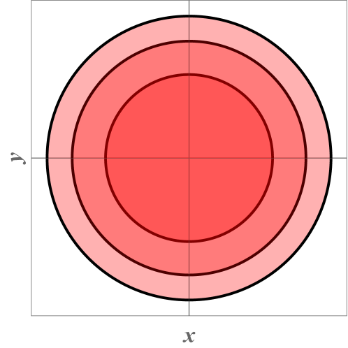
Figure 1: Schematic top view of the fermions in 2d, showing the “wedding cake” structure of the density. In this figure there are $k_{\max}=3$ layers, with darker shaded areas corresponding to higher density.

More precisely, in the window

$$\frac{(k_{\max}-1)k_{\max}}{N}<1-\Omega<\frac{k_{\max}(k_{\max}+1)}{N}$$ (3)

where $k_{\max}\geq 1$ is a positive integer, the total number of layers is $k_{\max}$, and for each layer, the density has a plateau value at $\rho=\frac{k}{\pi}$, $k=1,\dots,k_{\max}$. Finally, when $k_{\max}=1$, there is a single layer left, of density height $1/\pi$ and radius $\sim N^{1/2}$ that corresponds to the LLL. While the wedding cake structure of the density in the vicinity of $\Omega=1$ was found in KulkarniRotating2020 , here we study in detail the full crossover from the finite $\Omega$ regime (spherical cap) to the uniform disk. Our study reveals that the quantum steps also occur in the FCS and in the entropy. More precisely, in the regime $1-\Omega=O(1/N)$, we unveil a very useful mapping onto a 1d harmonic oscillator, which allows to compute easily not only the steps in the density, but also the corresponding piecewise linear form of all the cumulants of the number of fermions in a fixed circular domain, as well as the associated entanglement entropy. Although we restrict here to the harmonic potential, this mapping is in principle versatile enough to treat more general external radial potentials such that the system remains near the LLL, and to exhibit the universal features.

II Rotating harmonic oscillator in 2d: general framework

Let us start with the 2d geometry. The single particle Hamiltonian reads in polar coordinates $(r,\phi)$

$$H=-\frac{1}{2}\left(\partial_{r}^{2}+\frac{1}{r}\partial_{r}+\frac{1}{r^{2}}\partial_{\phi}^{2}\right)+V(r)-\Omega\frac{1}{i}\partial_{\phi}\,.$$ (4)

Decomposing on the sectors of angular momentum $\ell$, i.e. the eigenfunctions are $\psi_{n,\ell}(r,\phi)=r^{-1/2}\chi_{n,\ell}(r)\frac{e^{i\ell\phi}}{\sqrt{2\pi}}$ with $\ell\in\mathbb{Z}$, where the $\chi_{n,\ell}(r)$ are eigenfunctions of the radial Hamiltonian $\hat{H}_{\ell}$ with effective radial potential $V_{\ell}(r)$

$$\hat{H}_{\ell}=-\frac{1}{2}\partial_{r}^{2}+V_{\ell}(r)\;,\quad V_{\ell}(r)=V(r)+\frac{\ell^{2}-\frac{1}{4}}{2r^{2}}-\Omega\ell\;,$$ (5)

see LandauLifshitz ; Verbaarschot2002 ; KulkarniRotating2020 .

From now on we focus on the case of the harmonic potential $V(r)=\frac{r^{2}}{2}$, until said otherwise below. We use units such that $\omega=1$, $\Omega$ being now dimensionless. The eigenfunctions read $\psi_{n,\ell}(r,\phi)=a_{n,\ell}L_{n}^{|\ell|}(r^{2})r^{|\ell|}e^{-r^{2}/2}e^{i\ell\phi}$, where $L_{n}^{\alpha}(x)$ are the associated Laguerre polynomials, $a_{n,\ell}^{2}=\frac{\Gamma(1+n)}{\pi\Gamma(1+n+|\ell|)}$ and the eigenenergies are

$$\epsilon_{n,\ell}=2n+1+|\ell|-\Omega\ell\quad,\quad n=0,1,\dots\,$$ (6)

Consider now the ground state of $N$ noninteracting fermions. It is constructed as a Slater determinant over the $N$ lowest energy eigenstates, by filling all energy levels with $\epsilon_{n,\ell}\leq\mu$, where $\mu$ is the Fermi energy. Let us denote by $m_{\ell}$ the number of fermions in the sector $\ell$. It is equal to the number of values of $n=0,1,2,\dots$ such that $2n+1+\left[1-\Omega\,\text{sgn}\left(\ell\right)\right]\ell\leq\mu$ where $\text{sgn}\left(\ell\right)$ is the sign function. This leads to

$$m_{\ell}=\begin{cases}{\rm Int}\left(\dfrac{\mu+1-(1-\Omega)\ell}{2}\right)\quad,&\ell\geq 0\\[17.07164pt] {\rm Int}\left(\dfrac{\mu+1+(1+\Omega)\ell}{2}\right)\quad,&\ell\leq 0\end{cases}$$ (7)

where ${\rm Int}(x)$ denotes the integer part of $x$. This construction is illustrated in Fig. 2. Finally the relation between $N$ and $\mu$ is given by $\sum_{\ell}m_{\ell}=N$.

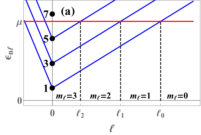
Figure 2: (a) Schematic plot of the spectrum $\epsilon_{n,\ell}=2n+1+|\ell|-\Omega\ell$ for $0<\Omega<1$ as a function of the angular quantum number $\ell=0,1,\dots$ for the levels $n=0,1,2,3,\dots$ (blue solid lines, of slopes respectively $-1-\Omega$ ($\ell<0$) and $1-\Omega$ ($\ell>0$). The condition $\epsilon_{n,\ell}\leq\mu$ determines the states which are occupied in the ground state. For a given $\ell$, the states with $n=0,\dots,m_{\ell}-1$ are occupied. (b) Schematic plot of $m_{\ell}$ versus $\ell$ which exhibits jumps at the values $\ell_{k}$ defined below, in Eq. (IV.2) (which are not necessarily integers).

Assuming $\mu\geq 1$ we see from (7) that $m_{\ell}\geq 1$ for $\ell_{\rm min}\leq\ell\leq\ell_{\rm max}$ with

$$\ell_{\rm max}={\rm Int}\left(\frac{\mu-1}{1-\Omega}\right)\;,\quad\ell_{\rm min}=-{\rm Int}\left(\frac{\mu-1}{1+\Omega}\right)\;,$$ (8)

and $m_{\ell}=0$ outside of this interval. Hence we see that when $\Omega\to 1^{-}$ and $\mu\geq 1$ many states are occupied on the branch $\ell\geq 0$ and few on the branch $\ell<0$, see Fig. 2. When $m_{\ell}=1$ for all $\ell<\ell_{0}$ only the LLL is filled, a situation to which we will return below.

Once the set of $m_{\ell}$ are known, the FCS for the number ${\cal N}_{R}$ of fermions in a disk of radius $R$ centered on the origin can be obtained from those of a collection of 1d problems in each angular sector. Indeed, one can show, see e.g. UsCounting2020 , that the FCS generating function can be simply written as a product

$$\left\langle e^{-s{\cal N}_{R}}\right\rangle=\prod_{\ell}\left\langle e^{-s{\cal N}_{[0,R]}}\right\rangle_{V_{\ell},m_{\ell}}$$ (9)

i.e. that the quantum fluctuations decouple in the different angular sectors. Here ${\cal N}_{[0,R]}$ is the number of fermions in the interval $[0,R]$ for a 1d problem of $m_{\ell}$ fermions in their ground state with Hamiltonian $\hat{H}_{\ell}$ (i.e. in the potential $V_{\ell}(r)$), see Eq. (5). Note that one can explicitly write the bounds $\ell_{\rm min}\leq\ell\leq\ell_{\rm max}$ on the product (9), or ignore it, since the factors are unity when $m_{\ell}=0$. In the following we analyze the consequences of this formula in various situations. In particular taking the logarithm of (9) and expanding in $s$ we see that each cumulant of ${\cal N}_{R}$ is the sum of the cumulants of the $1d$ problems associated to the different $\ell$ sectors, i.e. for any integer $p\geq 1$ one has footnote:pCumulant

$$\left\langle{\cal N}_{R}^{p}\right\rangle^{c}=\sum_{\ell=\ell_{{\rm min}}}^{\ell_{{\rm max}}}\left\langle{\cal N}_{[0,R]}^{p}\right\rangle_{V_{\ell},m_{\ell}}^{c}\;.$$ (10)

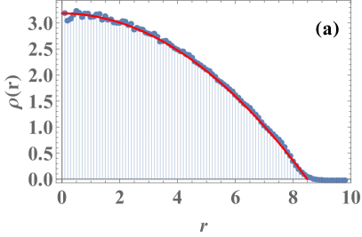
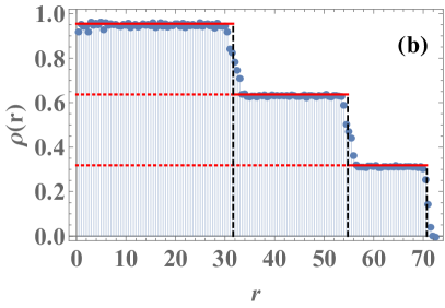
Figure 3: Density of the particles for $N$ fermions in a rotating harmonic trap in the two regimes (a) $1-\Omega=O(1)$ and (b) $1-\Omega=O(1/N)$. Solid red line: theoretical predictions, Eq. (13) in (a) Eq. (46) in (b). In (b), the black dashed lines correspond to $R=\sqrt{\ell_{k}}$, and the red dotted lines are the continuations of the formula (46) to $r=0$. Blue bars: the density computed empirically from numerical simulations. Parameters are $\Omega=2/3$, $\mu=20$ corresponding to a total of $N=366$ fermions in (a), and $\Omega=0.999$ and Fermi energy $\mu=6$, corresponding to $N=9003$ in (b). The number of samples was $5000$ in (a) and $200$ in (b).

III Rotating harmonic oscillator in 2d: the case $0<\Omega<1$

III.1 FCS in the regime $0<\Omega<1$ with large $N$

We consider the limit of large $N$, with a fixed value of the angular frequency $0\leq\Omega<1$, which implies large $\mu$. Let us first determine the relation between $N$ and $\mu$, as well as the mean fermion density $\rho({\bf r})$ in the ground state, which in this problem, by rotational symmetry, is only a function of $r=|{\bf r}|$, i.e.,

$$\int d^{2}{\bf r}\,\rho({\bf r})=N\;,\quad\rho({\bf r})=\rho(r)\;.$$ (11)

In that regime each angular sector has a macroscopic occupation number $m_{\ell}=O(\mu)$ (see below). One can approximate $V_{\ell}(r)\simeq V_{\ell}^{0}(r)=\frac{r^{2}}{2}+\frac{\ell^{2}}{2r^{2}}-\Omega\ell$ and $m_{\ell}\simeq\frac{\mu+\Omega\ell-|\ell|}{2}$. We will use the fact that for large $\mu,N$ the values of $\ell$ which dominate the sum $N=\sum_{\ell=\ell_{\rm min}}^{\ell_{\rm max}}m_{\ell}$ are $\ell=O(\mu)$ with $m_{\ell}=O(\mu)$. The relation between $\mu$ and $N$ becomes

$$N\simeq\int_{-\frac{\mu}{1+\Omega}}^{\frac{\mu}{1-\Omega}}d\ell\,\frac{\mu+\Omega\ell-|\ell|}{2}=\frac{\mu^{2}}{2(1-\Omega^{2})}\;.$$ (12)

On the other hand the mean fermion density in that regime is given by the semi-classical/LDA method (see Appendix A for details)

$$\rho({\bf r})\simeq\frac{k_{F}(r)^{2}}{4\pi}=\frac{2\mu-(1-\Omega^{2})r^{2}}{4\pi}=\frac{2N}{\pi R_{e}^{2}}\left[1-\left(\frac{r}{R_{e}}\right)^{2}\right]$$ (13)

in the disk $r<R_{e}$ where

$$R_{e}=\sqrt{\frac{2\mu}{1-\Omega^{2}}}\simeq\sqrt{2}\left(\frac{2N}{1-\Omega^{2}}\right)^{1/4}\,,$$ (14)

and zero outside the disk, $R>R_{e}$. One can check using $N=\int d^{2}{\bf r}\rho({\bf r})$ that (12) is satisfied. Eq. (13) shows good agreement with the numerical simulations, see Fig. 3 (a) (the technical details of the simulations are given in Appendix E).

Let us now return to the random variable ${\cal N}_{R}$. Its mean value is given to leading order by $\left\langle{\cal N}_{R}\right\rangle=\int_{r<R}d^{2}{\bf r}\rho({\bf r})\simeq N\left(\frac{R}{R_{e}}\right)^{2}\left[2-\left(\frac{R}{R_{e}}\right)^{2}\right]$, from (13). We now study its fluctuations, and compute the variance. From (10), the variance in this regime is given by

$${\rm Var}\,{\cal N}_{R} = \sum_{\ell=-\ell_{{\rm\min}}}^{\ell_{{\rm max}}}\,\left.{\rm Var}\,{\cal N}_{[0,R]}\right|_{V_{\ell},m_{\ell}}$$ (15)

$$\simeq \int_{-\frac{\mu}{1+\Omega}}^{\frac{\mu}{1-\Omega}}\,d\ell\,\left.{\rm Var}\,{\cal N}_{[0,R]}\right|_{V_{\ell}^{0}(r),m_{\ell}}\;.$$

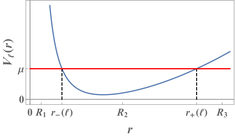
Figure 4: Plot of the 1d potential $V_{\ell}(r)$ versus $r$ associated to a given angular sector $\ell$. For a large number of fermions $m_{\ell}=O(\mu)$ in their ground state the support of the density $[r_{-}(\ell),r_{+}(\ell)]$ is shown. The positions of the edges $r_{\pm}(\ell)$ correspond to the roots of $V_{\ell}(r)=\mu$. Three cases are represented $R<r_{-}(\ell)$, $R\in[r_{-}(\ell),r_{+}(\ell)]$ and $R>r_{+}(\ell)$. In the first and last cases the fluctuations of ${\cal N}_{[0,R]}$ are negligible since ${\cal N}_{[0,R]}\simeq 0$ or $N$ respectively.

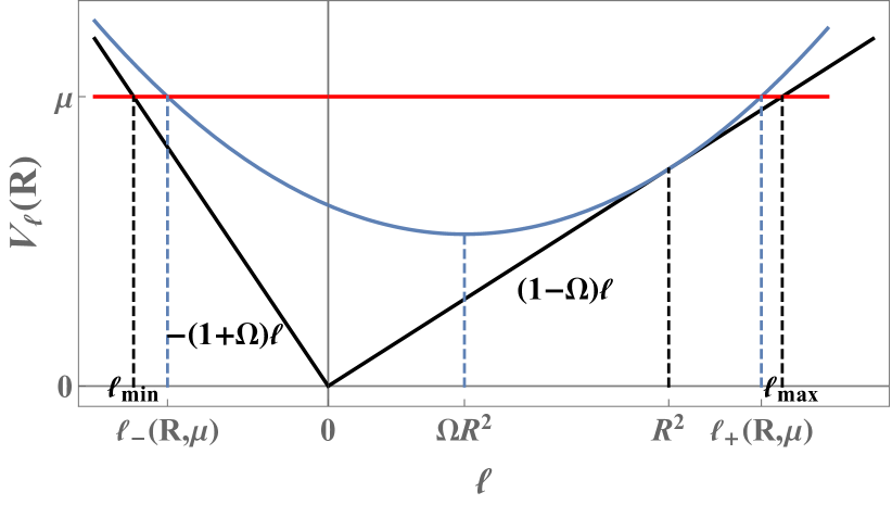
Figure 5: On the same plot: (i) $\epsilon_{0,\ell}$ versus $\ell$, i.e. the two black solid lines with slopes $1-\Omega$ and $-(1+\Omega)$ respectively. Their intersections with the level $\mu$ determine $\ell_{\rm max}$ and $\ell_{\rm min}$ defined in Eq. (8). The distance between that level to the lines equals twice the number $m_{\ell}$ of occupied states in the ground state, see Eq. (7). (ii) For a given $R$, $V_{\ell}\left(R\right)\simeq\frac{R^{2}}{2}+\frac{\ell^{2}}{2R^{2}}-\Omega\ell$ versus $\ell$ (solid blue line), is a parabola which is tangent to both lines at $\ell=\pm R^{2}$. The intersections between $V_{\ell}\left(R\right)$ and the level $\mu$ determine the actual range of integration $\ell_{\pm}(R,\mu)$ which we use to calculate ${\rm Var}\,{\cal N}_{R}$, see Eqs. (16) and (III.1).

We can now use the results derived in UsCounting2020 for ${\rm Var}\,\left.{\cal N}_{[0,R]}\right|_{V_{\ell}^{0}(r),m_{\ell}}$, i.e. for the 1d inverse square potential well $V^{0}_{\ell}(r)$. In this potential we consider $m_{\ell}=O(\mu)$ fermions, and the 1d fermion density vanishes outside the interval $[r_{-}(\ell),r_{+}(\ell)]$, where $r_{\pm}(\ell)$ are the two roots of $V^{0}_{\ell}(r)=\mu$. As shown in Figure 4, for a fixed $\mu$ and $R$, the integrand in (15) is nonnegligible only if $R$ is inside the interval $[r_{-}(\ell),r_{+}(\ell)]$, which is equivalent to $\ell\in[\ell_{-}(R),\ell_{+}(R)]$ where $\ell_{\pm}(R)$ are the two roots of $V^{0}_{\ell}(R)=\frac{1}{2}R^{2}+\frac{\ell^{2}}{2R^{2}}-\Omega\ell=\mu$, i.e.

$$\ell_{\pm}(R)=\Omega R^{2}\pm R\sqrt{2\mu-(1-\Omega^{2})R^{2}}\;.$$ (16)

One can check that $\left[\ell_{-}(R),\ell_{+}(R)\right]\subset\left[\ell_{{\rm min}},\ell_{{\rm max}}\right]$, see Fig. 5. We use the equation (18) of UsCounting2020 with the replacement $a\to R$, $\alpha\to\ell$, $N\to m_{\ell}$ and $\mu\to\mu+\Omega\ell$, leading to

$$2\pi^{2}{\rm Var}\,{\cal N}_{R}\simeq$$

$$\int_{\ell_{-}(R)}^{\ell_{+}(R)}d\ell\left[\log\left(R\frac{\left(2\mu-\left(R^{2}+\frac{\ell^{2}}{R^{2}}-2\Omega\ell\right)\right)_{+}^{3/2}}{\left((\mu+\Omega\ell)^{2}-\ell^{2}\right)_{+}^{1/2}}\right)+c_{2}\right]$$

with $c_{2}=\gamma_{E}+1+\log 2$, where $\gamma_{E}$ is Euler’s constant. To be accurate we must stress that this formula holds in the following sense. Define the scaled radius $\tilde{R}=R/\sqrt{2\mu}$. Then in the limit of large $\mu$ with fixed $\tilde{R}$ and $\Omega$, we obtain our main result for the variance

$${\rm Var}\,{\cal N}_{R}=A_{\tilde{R},\Omega}\mu\log\mu+B_{\tilde{R},\Omega}\mu+o(\mu)\,,$$ (18)

$$A_{\tilde{R},\Omega}=\frac{2}{\pi^{2}}\tilde{R}\sqrt{1-(1-\Omega^{2})\tilde{R}^{2}}\,,$$ (19)

$$B_{\tilde{R},\Omega}=\int_{\lambda_{-}(\tilde{R})}^{\lambda_{+}(\tilde{R})}\frac{d\lambda}{2\pi^{2}}$$

$$\quad\times\left[\log\left(4\tilde{R}\frac{(1-(\tilde{R}^{2}+\frac{\lambda^{2}}{4\tilde{R}^{2}}-\Omega\lambda))_{+}^{\frac{3}{2}}}{((1+\Omega\lambda)^{2}-\lambda^{2})_{+}^{\frac{1}{2}}}\right)+c_{2}\right],$$ (20)

where $\lambda_{\pm}=2\tilde{R}\left(\Omega\tilde{R}\pm\sqrt{1-(1-\Omega^{2})\tilde{R}^{2}}\right)$. The integral in the formula for $B_{\tilde{R},\Omega}$ can be performed and is displayed in (113). Note that in the scaled variables the position of the edge is $\tilde{R}_{e}=\frac{1}{\sqrt{1-\Omega^{2}}}>1$ (the rotation expands the Fermi gas). Alternatively one can express (18)-(III.1) in terms of $N$ and $R/R_{e}$ using (12) and $\tilde{R}=R/(R_{e}\sqrt{1-\Omega^{2}})$. In Fig. 6 (a), the numerical simulations of ${\rm Var}\,{\cal N}_{R}$ are compared with the prediction of (18), showing excellent agreement.

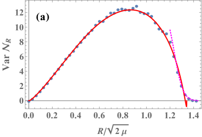
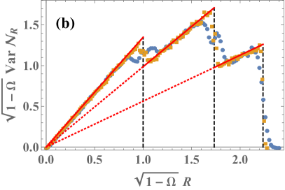
Figure 6: Variance of the number of fermions in a disk of radius $R$ for a 2d rotating harmonic trap, in the two regimes (a) $1-\Omega=O(1)$ and (b) $1-\Omega=O(1/N)$. The symbols are the variance computed empirically over ${10}^{4}$ simulations. The red solid lines are the theoretical predictions (18) in (a) and (50) in (b), and the magenta dotted line in (a) is the edge prediction (31). In (b), the black dashed lines correspond to $R=\sqrt{\ell_{k}}$ and the red dotted lines are the continuations of the formula (50) to the origin. Parameters are: (a) $\Omega=2/3$ and $\mu=20$ corresponding to $N=366$ and (b) Fermi energy $\mu=6$ and $\Omega=0.99$ (blue circles) and $\Omega=0.999$ (yellow squares), corresponding to $N=903$ and $N=9003$ fermions respectively. The agreement between the theory and simulations is good except for boundary layers around $R=\sqrt{\ell_{k}}$ in (b), which are treated below, see, e.g., Fig. 7. As seen in the figure, these boundary layers become narrower as $N$ is increased such that (50) becomes exact in the limit $N\to\infty$ limit.

It is also interesting to study the $p^{\rm th}$ cumulant of ${\cal N}_{R}$, i.e. $\left\langle{\cal N}_{R}^{p}\right\rangle^{c}$, beyond the variance, which corresponds to $p=2$. By the same small scale universality arguments as in Ref. UsCounting2020 , we obtain (for arbitrary integer $m>1$)

$$\left\langle{\cal N}_{R}^{2m}\right\rangle^{c}=2\mu\tilde{R}\sqrt{1-(1-\Omega^{2})\tilde{R}^{2}}\,\left(\kappa_{2m}+o(\mu)\right)\;,$$ (21)

with

$$\kappa_{2m}={(-1)^{m+1}(2m)!2\zeta(2m-1)}/{(m(2\pi)^{2m})}$$ (22)

while the odd cumulants vanish to $O(\mu)$.

III.2 Edge regime for $1-\Omega=O(1)$

We now calculate the number variance for $R\simeq R_{e}$ near the edge of the Fermi gas in the regime $1-\Omega=O(1)$. Our result (18) breaks down near the edge, because it was obtained using approximations that are only valid in the bulk.

For $1d$ systems, the statistical properties near the edge of Fermi gases are determined by the Airy kernel

$$K_{\rm Ai}(x,y)=\frac{{\rm Ai}(x){\rm Ai}^{\prime}(y)-{\rm Ai}^{\prime}(x){\rm Ai}(y)}{x-y}\,.$$ (23)

In particular, the number variance for a semi-infinite interval beginning (or ending) around the edge of the gas follows a known universal behavior which depends only on the derivative of the potential at the edge MMSV14 ; MMSV16 . Applying these known results to each of the sectors, we have

$$\left.{\rm Var}\,{\cal N}_{[0,R]}\right|_{V_{\ell}^{0}(r),m_{\ell}}\simeq\frac{1}{2}\mathcal{V}_{2}\left(\frac{R-r_{+}\left(\ell\right)}{w\left(\ell\right)}\right)$$ (24)

where $w\left(\ell\right)=\left[2\left(V_{\ell}^{0}\right)^{\prime}\left(r_{+}\right)\right]^{-1/3}$ and the universal scaling function is MMSV14 ; MMSV16

$${\cal V}_{2}(\hat{a}):={2}\int_{\hat{a}}^{+\infty}du\int_{-\infty}^{\hat{a}}dvK_{\text{Ai}}^{2}\left(u,v\right)\,.$$ (25)

These results are valid when the argument of ${\cal V}_{2}$ in (24) is of order unity.

We now wish to use (24) in (15) in the regime $R\simeq R_{e}$. The dominant contribution to ${\rm Var}\,{\cal N}_{R}$ is from $\ell\simeq\ell_{e}$ where $r_{+}\left(\ell_{e}\right)=R_{e}$ and therefore, plugging (24) directly into (15) gives the correct leading-order result. Using (16) with $R=R_{e}=\sqrt{\frac{2\mu}{1-\Omega^{2}}}$, we find that $\ell_{e}=\Omega R_{e}^{2}=2\mu\Omega/\left(1-\Omega^{2}\right)$. At $\ell\simeq\ell_{e}$,

$$\!\!\!w\left(\ell\right) \simeq w\left(\ell_{e}\right)=\left[2\left(V_{\ell_{e}}^{0}\right)^{\prime}\left(R_{e}\right)\right]^{-1/3}$$ (26)

$$= \left[2\left(R_{e}-\frac{\ell_{e}^{2}}{R_{e}^{3}}\right)\right]^{-1/3}\!=\left[8\mu\left(1-\Omega^{2}\right)\right]^{-1/6}.$$

Summarizing, we have so far

$${\rm Var}\,{\cal N}_{R}\simeq\int_{-\frac{\mu}{1+\Omega}}^{\frac{\mu}{1-\Omega}}\,d\ell\,\frac{1}{2}\mathcal{V}_{2}\left(\frac{R-r_{+}\left(\ell\right)}{w\left(\ell_{e}\right)}\right)\,.$$ (27)

Solving the equation $V_{\ell}^{0}\left(r_{+}\right)=\mu$, we find

$$r_{+}^{2}=\left(\Omega\ell+\mu\right)+\sqrt{\left(\Omega\ell+\mu\right)^{2}-\ell^{2}}$$ (28)

which, in the vicinity of $\ell=\ell_{e}$ (and $r_{+}=R_{e}$), yields

$$r_{+}\simeq R_{e}-\frac{\sqrt{1-\Omega^{2}}}{4\sqrt{2}\,\mu^{3/2}}\left(\ell-\ell_{e}\right)^{2}\,.$$ (29)

Plugging (29) into (27), we find that the dominant contribution to the integral comes from $\ell\simeq\ell_{e}$ and therefore the integration limits can be replaced by plus and minus infinity:

$${\rm Var}\,{\cal N}_{R}\simeq\int_{-\infty}^{\infty}\!\!d\ell\,\frac{1}{2}\mathcal{V}_{2}\left(\frac{R-R_{e}}{w\left(\ell_{e}\right)}+\frac{\sqrt{1-\Omega^{2}}\,\left(\ell-\ell_{e}\right)^{2}}{4\sqrt{2}\,\mu^{3/2}w\left(\ell_{e}\right)}\right)\,.$$ (30)

Now, we change the integration variable to $\xi=\frac{\sqrt{1-\Omega^{2}}}{4\sqrt{2}\,w\left(\ell_{e}\right)\mu^{3/2}}\left(\ell-\ell_{e}\right)^{2}$, noting that the two sides $\ell>\ell_{e}$ and $\ell<\ell_{e}$ produce identical results, leading to an extra factor of $2$. Simplifying, we obtain finally the scaling form for the variance at the edge in the regime $\Omega<1$

$${\rm Var}\,{\cal N}_{R}\simeq\frac{\mu^{2/3}}{\left(1-\Omega^{2}\right)^{1/3}}\int_{0}^{\infty}\,\frac{d\xi}{\sqrt{\xi}}\mathcal{V}_{2}\left(\hat{R}+\xi\right)$$ (31)

where $\hat{R}=\frac{R-R_{e}}{w\left(\ell_{e}\right)}$. In the nonrotating case $\Omega=0$, Eq. (31) coincides with the result of UsCounting2020 .

III.3 Entanglement entropy in the bulk

We now apply our results to the calculation of the bipartite Rényi entanglement entropy of a disk $D_{R}$ of radius $R$ centered around the origin with its complement $\overline{D}_{R}$. For any domain $\mathcal{D}$, its definition, parametrized by $q\geq 1$, is given by

$$S_{q}({\cal D})=\frac{1}{1-q}\log\operatorname{Tr}[\hat{\rho}_{\cal D}^{q}],$$ (32)

where the reduced density matrix is given by $\hat{\rho}_{\cal D}=\operatorname{Tr}_{\overline{\cal D}}[\hat{\rho}]$, i.e., tracing out the density matrix $\hat{\rho}$ of the system over $\overline{\cal D}$. In the limit $q\to 1$ one recovers the von Neumann entropy $S_{1}=-\text{Tr}\left[\hat{\rho}_{{\cal D}}\log\hat{\rho}_{{\cal D}}\right]$. A remarkable fact is that for noninteracting fermions one can express $S_{q}({\cal D})$ as a series in the (even) cumulants of ${\cal N}_{\cal D}$,

$$S_{q}({\cal D})=\sum_{m\geq 1}s_{m}^{(q)}\left\langle{\cal N}_{{\cal D}}^{2m}\right\rangle^{c},$$ (33)

where the coefficients $s_{m}^{(q)}$ are given in CMV2012 and $s_{1}^{(q)}=\frac{\pi^{2}}{6}(1+\frac{1}{q})$.

For a disk of radius $R$, in the regime $\Omega=O(1)$ we use our expressions (18) for the variance and (21) for the higher cumulants to obtain

$$S_{q}\left(D_{R}\right) = \frac{\pi^{2}\left(q+1\right)}{6q}{\rm Var}\,{\cal N}_{R}$$ (34)

$$+ 2\mu\tilde{R}\sqrt{1-(1-\Omega^{2})\tilde{R}^{2}}\,\tilde{E}_{q}+o(\mu)$$

where $\tilde{E}_{q}=\sum_{m\geq 2}s_{m}^{(q)}\kappa_{2m}=E_{q}-\frac{q+1}{6q}(1+\gamma_{E})$ and $E_{q}$ is given explicitly in Eq. (11) in CalabreseEntropyFreeFermions (see also JinKorepin2004 ). In (34) the simple form of the second term arises from the common $R$ dependence of the cumulants of order $4$ and higher. For the nonrotating case $\Omega=0$, the result (34) is in agreement with UsCounting2020 .

Note that in the other regime $\Omega\to 1$, the entanglement entropy in the lowest Landau level $k=1$ was obtained directly from the overlap matrix in LMG19 . Since all the cumulants are linear in $R$, the entropy was also found to be linear in $R$ in the bulk (see also Refs. RS09 ; CE19 ; LSS20 for studies of the entanglement entropy in that regime). We will return to this point in the next section.

IV Rotating harmonic oscillator in 2d: the case $1-\Omega\to 0$

We now address the limit $\Omega\to 1^{-}$ and, in the large $N$ limit, the regime $1-\Omega=O(1/N)$. As described in the Introduction, a sequence of transitions occurs in this regime, corresponding to filling successive Landau levels, at discrete values of $\Omega$ given by (3) (see also (41) below with $n=k_{\max}$). We first address the case of a single LLL, where the density is uniform in a disk, and in a second stage we decrease $\Omega$, which results in higher Landau levels being occupied and new layers being formed, see Fig. 1.

IV.1 LLL and FCS in the regime $\Omega\to 1^{-}$

Let us first recall the case $1-\frac{2}{N-1}<\Omega<1$ where the ground state is constructed from single particle states in the LLL (i.e. the branch $n=0$ in Fig. 2. This case is related to the Ginibre ensemble of random matrices LMG19 . Here, as a benchmark for our method, we show how to recover the results of LMG19 using a different eigenbasis for single particle states. From Fig. 2 we see that the occupied energy levels in the ground state are $\epsilon_{0,\ell}=1+(1-\Omega)\ell$ for $\ell=0,\dots,N-1$, i.e. no states on the branch $\ell<0$ are occupied and the occupied states on the branch $\ell\geq 0$ all contain a single fermion, $m_{\ell}=1$. For a single fermion in an inverse square potential it is easy to obtain the probability that the fermion is in $[0,R]$ from its wave function $\psi_{0,\ell}$. From (9) one then immediately obtains the FCS generating function as

$$\left\langle e^{-s{\cal N}_{R}}\right\rangle = \prod_{\ell=0}^{N}\left\langle e^{-s{\cal N}_{[0,R]}}\right\rangle_{V_{\ell},m_{\ell}=1}$$

$$= \prod_{\ell=0}^{N}\int_{0}^{+\infty}\left[1-\left(1-e^{-s}\right)\int_{0}^{R}\chi_{0\ell}(r)^{2}dr\right]$$

with $\chi_{0\ell}(r)=\sqrt{\frac{2}{|\ell|!}}r^{|\ell|+\frac{1}{2}}e^{-r^{2}/2}$. Taking the logarithm one finds the cumulants

$$\sum_{p=0}\!\frac{(-s)^{p}}{p!}\!\left\langle{\cal N}_{R}^{p}\right\rangle^{c}\!=\!\sum_{\ell=0}^{N-1}\!\log\!\left(1-(1-e^{-s})\frac{\gamma\left(\ell+1,R^{2}\right)}{\Gamma(\ell+1)}\right)$$ (36)

where $\gamma(a,z)=\int_{0}^{z}t^{a-1}e^{-t}dt$, recovering Eq. (31) in the supplemental material of LMG19 .

These results are exact for any $N$. In the large $N$ limit this corresponds to taking the limit $\Omega\to 1^{-}$ with $\Omega$ in the window $1-\frac{2}{N}<\Omega<1$. In that regime, the analysis of (IV.1) performed in LMG19 shows that the cumulants grow linearly with the radius of the disk $R$ as

$$\left\langle{\cal N}_{R}^{p}\right\rangle^{c}\simeq B_{1}^{(p)}R$$ (37)

where the $B^{(p)}_{1}$ are numbers obtained in LMG19 with $B^{(2)}_{1}={1}/{\sqrt{\pi}}$.

IV.2 Vicinity of the LLL and $\Omega\to 1$ limit

We now explore the vicinity of the LLL, focusing on the large $N$ limit with $1-\Omega=O(1/N)$. We unveil a mapping to a 1d harmonic oscillator, Eq. (42) below, which allows to easily compute the steps in the density (the ”wedding cake”) and to obtain the corresponding quantum step structure for the FCS.

We first discuss the filling of the Landau levels. It is equivalent to decrease $\Omega$ at fixed $N$ or to increase the Fermi energy $\mu$ for a fixed $\Omega$. Let us focus first on the latter and denote by $n\geq 0$ the integer for which

$$2n+1<\mu<2n+3\,.$$ (38)

Consider the energy levels with $\ell\geq 0$. The level $\epsilon_{n,\ell}$ is occupied if $2n+1+(1-\Omega)\ell\leq\mu$. Hence we find that $m_{\ell}$ is a decreasing integer staircase (see figure 2), with $m_{0}=n+1=m_{\ell}$ for $\ell<\ell_{n}=\frac{\mu-(2n+1)}{1-\Omega}$, and $m_{\ell}=0$ for $\ell>\ell_{0}=\frac{\mu-1}{1-\Omega}$, more generally

$$m_{\ell}=k\quad,\quad\ell_{k}<\ell<\ell_{k-1}\quad,\quad k=n+1,\dots,0$$

$$\ell_{k}=\frac{\mu-(2k+1)}{1-\Omega}$$ (39)

where the $\ell_{k}$ are not necessarily integers. The LLL case is obtained for $n=0$, i.e. $1<\mu<3$, in which case $m_{\ell}=1$ for $\ell<\ell_{0}=\frac{\mu-1}{1-\Omega}$. Since we want the states with $\ell=0,\dots,N-1$ to be occupied we need $\ell_{0}>N-1$ hence $1-\Omega<(\mu-1)/(N-1)$, which for large $N$ leads to the window $1-\frac{2}{N}<\Omega<1$ identified above and studied in LMG19 . As we show below the cases $n=1,2,\dots$ lead to a structure similar, but slightly different to the ”wedding cake” of KulkarniRotating2020 , where the number of layers decreases as $\ell$ increases. To compute the relation between $\mu$ and $N$ we note that the total number $N_{\geq}$ of occupied states for $\ell\geq 0$ is

$$N_{\geq} \simeq (n+1)\ell_{n}+n(\ell_{n+1}-\ell_{n})+\dots$$ (40)

$$= \sum_{k=0}^{n}\ell_{k}=\frac{(n+1)(n+\mu^{\prime})}{1-\Omega}$$

with $\mu^{\prime}=\mu-(2n+1)\in]0,2[$ [see Eq. (38)]. Since in that regime the number $N_{<}$ of occupied states with $\ell<0$ is only $O(1)$ it can be neglected so $N\simeq N_{\geq}$ hence the regime (38) is equivalent to

$$\frac{n(n+1)}{N}<1-\Omega<\frac{(n+1)(n+2)}{N}$$ (41)

This is the large $N$ regime on which we focus here. In that case $\mu=O(1)$ and the size of Fermi gas is of order $R_{e}\sim\sqrt{N}$, see below.

We now discuss the statistics of ${\cal N}_{R}$ in that regime, i.e. described by (38), (41) with $n$ a fixed integer and $N$ large. A first simplification is that it can be mapped to a 1d harmonic oscillator problem. Indeed, we see that the $\ell_{k}$ are typically $O(N)$. One can check that for large $\ell$ the potential $V_{\ell}(r)$ in (5) is very well approximated around its minimum at $r=r^{*}(\ell)$ by a quadratic potential. In the present case of the harmonic oscillator (HO), $V(r)=\frac{1}{2}r^{2}$ one finds $r^{*}(\ell)=\sqrt{\ell}$ and denoting $r=r^{*}(\ell)+u$ one obtains the expansion

$$V_{\ell}\left(r=\sqrt{\ell}+u\right)\simeq\left(1-\Omega\right)\ell+2u^{2}+O\left(u^{3}/\sqrt{\ell},u^{4}/\ell\right)\,.$$ (42)

Thus we can approximate the original Hamiltonian $H_{\ell}$ in each angular sector by a harmonic oscillator with Hamiltonian $H_{1d\rm{HO}}=-\frac{1}{2}\frac{\partial^{2}}{\partial u^{2}}+2u^{2}$. As a consequence [see Eq. (42)] we have $\left.{\cal N}_{[0,R]}\right|_{V_{\ell}(r),m_{\ell}}\simeq\left.{\cal N}_{\left[-\sqrt{\ell},R-\sqrt{\ell}\right]}\right|_{2u^{2},m_{\ell}}$, where the subscripts in the last quantity indicated that it is calculated in the ground state of $H_{1d\rm{HO}}$ with $m_{\ell}$ fermions.

Let us begin by calculating the density $\rho\left({\bf r}\right)\equiv\rho\left(r\right)$, which is related to the mean of ${\cal N}_{R}$ via $\frac{d\left\langle{\cal N}_{R}\right\rangle}{dR}\big{|}_{R=r}=2\pi r\rho\left(r\right)$. We consider here $R=O(\sqrt{N})$, i.e. $\tilde{R}=O(1)$. Denoting by $\rho_{1d\text{HO},k}\left(u\right)$ the mean density for $k$ noninteracting fermions in the ground state of $H_{1d\rm{HO}}$ one has

$$\left\langle{\cal N}_{R}\right\rangle \simeq \sum_{k=1}^{n+1}\int_{\ell_{k}}^{\ell_{k-1}}d\ell\,\left\langle\left.{\cal N}_{\left[-\sqrt{\ell},R-\sqrt{\ell}\right]}\right|_{2u^{2},k}\right\rangle\,,$$ (43)

$$2\pi r\rho\left(r\right) \simeq \sum_{k=1}^{n+1}\int_{\ell_{k}}^{\ell_{k-1}}d\ell\,\rho_{1d\text{HO},k}\left(r-\sqrt{\ell}\right)\,.$$ (44)

We note now that for each value of $r$ only one value of $k$ contributes. Indeed the sizes of the staircase steps, $\sqrt{\ell_{k-1}}-\sqrt{\ell_{k}}$ being much larger than the width of the ground-state wavefunction of the harmonic oscillator (which is $O(1)$), for each $r$ the equivalent HO problem has a fixed number of fermions $k$ determined by $\sqrt{\ell_{k}}<r<\sqrt{\ell_{k-1}}$. Hence we have

$$2\pi r\rho\left(r\right)$$ (45)

$$\simeq 2r\,\theta\left(\sqrt{\ell_{k}}<r<\sqrt{\ell_{k-1}}\right)\int_{-\infty}^{+\infty}du\,\rho_{1d\text{HO},k}\left(u\right)$$

$$=2kr\quad,\quad\sqrt{\ell_{k}}<r<\sqrt{\ell_{k-1}}\;.$$ (46)

Since the width of the equivalent oscillator is fixed, to obtain (45) we changed the integration variable as $\sqrt{\ell}=r-u$ where $u$ varies of $O(1)$, and note that $d\ell=-2\left(r-u\right)du\simeq-2r\,du$. Finally, to reach Eq. (46) we used the normalization of the density for the 1d HO, $\int_{-\infty}^{+\infty}\rho_{1d\text{HO},k}\left(u\right)du=k$. Our prediction (46) for the density is compared with numerical simulations in Fig. 3 with excellent agreement. Note that the index $n+1$ in (41) gives the total number of Landau level which are occupied, while the index $k=1,\dots,n+1$ labels the plateaus in the density at $\rho(r)=k/\pi$, and correspond to a “local” droplet of a $k$-th Landau level. The density (46), describing a “wedding cake” structure, i.e. with plateaux at $\rho(r)=\frac{k}{\pi}$, was obtained in KulkarniRotating2020 in a more general setting footnote:density . They arrived at this result by first calculating the exact density and then performing an asymptotic analysis in the large-$N$ limit. They also studied the boundary layer form of the density around the edges of each plateau, at $r=\sqrt{\ell_{k}}$ where (46) breaks down. In Appendix C.1 we compute directly this boundary layer form using the harmonic approximation (42) and show that it is adequate in order to recover the result of KulkarniRotating2020 .

We now match the calculation of the density in the two regimes $\Omega=O(1)$ and $1-\Omega=O(1/N)$. We show that the corresponding formula for the density match when $\rho(r)=O(\mu)$. In the second regime, as we found above $\rho(r)=\frac{k}{\pi}$, where $k$ is obtained by inverting Eq. (IV.2), which gives $k\simeq\frac{\mu-\left(1-\Omega\right)\ell_{k}}{2}$. In the large $k$ limit one can approximate $\ell_{k}\sim r^{2}$ which leads to

$$\rho\left(r\right)\simeq\frac{\mu-\left(1-\Omega\right)r^{2}}{2\pi}\;.$$ (47)

It is easy to check that this is in agreement with Eq. (13) in the limit $1-\Omega\ll 1$, so the two regimes indeed match smoothly.

We now turn to the calculation of the variance of ${\cal N}_{R}$, following similar steps to those we used when we calculated the density in Eqs. (43)-(46). Using (15) and the HO approximation (42)

$${\rm Var}\,{\cal N}_{R}\simeq\sum_{k=1}^{n+1}\int_{\ell_{k}}^{\ell_{k-1}}\!d\ell\,{\rm Var}\left.{\cal N}_{\left[-\sqrt{\ell},R-\sqrt{\ell}\right]}\right|_{2u^{2},k}$$ (48)

$$\simeq 2R\,\theta\left(\sqrt{\ell_{k}}<R<\sqrt{\ell_{k-1}}\right)\!\int_{-\infty}^{+\infty}\!\!da\,{\rm Var}\left.{\cal N}_{(-\infty,a]}\right|_{2u^{2},k}\,,$$

where this time we used the change of variable $a=R-\sqrt{\ell}=O(1)$, with $\ell=O(N)$ at large $N$. We thus see that the variance is proportional to $R$ (the same applies to higher cumulants), and we will now calculate the prefactor. Using footnote:rescaling

$$\left.{\cal N}_{(-\infty,a]}\,\right|_{2u^{2},m_{\ell}}=\left.{\cal N}_{\left(-\infty,\sqrt{2}a\right]}\,\right|_{\frac{1}{2}u^{2},m_{\ell}}$$ (49)

we thus obtain that the variance is a discontinuous piecewise linear function

$${\rm Var}\,{\cal N}_{R}\simeq\sqrt{2}\,C_{k}R\quad,\quad\sqrt{\ell_{k}}<R<\sqrt{\ell_{k-1}}$$ (50)

where we recall that the $\ell_{k}$’s are given in (IV.2). Here the

$$C_{k}=\int_{-\infty}^{+\infty}da\,{\rm Var}\left.{\cal N}_{(-\infty,a]}\,\right|_{\frac{1}{2}u^{2},k}$$ (51)

are numbers that we have calculated in Appendix B. They are given by the explicit formula for integer $k\geq 1$

$$C_{k+1}=\frac{\Gamma(k+\frac{1}{2})^{2}}{\sqrt{2\pi}\pi k!^{2}}\,_{3}F_{2}\left(\frac{3}{2},-k,-k;\frac{1}{2}-k,\frac{1}{2}-k;1\right)$$ (52)

where ${}_{3}F_{2}\left(\cdots\right)$ denotes the hypergeometric function, with $C_{k}=\frac{1}{\sqrt{2\pi}}\{1,\frac{7}{4},\frac{153}{64},\dots\}$. In Fig. 6, numerical simulations of ${\rm Var}\,{\cal N}_{R}$ are compared with the prediction of (50). The agreement is good except in the boundary layers $R\simeq\sqrt{\ell_{k}}$. From the above formula we can extract the asymptotics of $C_{k}$ for large $k$, see Appendix B,

$$C_{k}\simeq\frac{\sqrt{2}}{\pi^{2}}\sqrt{k}\left(\log k+6\log 2+\gamma_{E}-2\right),\quad k\gg 1\,.$$ (53)

In Appendix C.2 we obtain the structure of the boundary layer describing the step at $R\simeq\sqrt{\ell_{k}}$. It takes the form

$${\rm Var}\,{\cal N}_{R}\simeq\sqrt{2}R\left[C_{k}+f_{k}^{\text{edge},\text{Var}}\left(\sqrt{2}\left(R-\sqrt{\ell_{k}}\right)\right)\right]$$ (54)

where the scaling function $f_{k}^{\text{edge},\text{Var}}(s)$ depends on $k$, and its exact expression for any $k\geq 0$ is given in (110). It is such that $f_{k}^{\text{edge},\text{Var}}\left(s\to-\infty\right)=C_{k+1}-C_{k}$, and $f_{k}^{\text{edge},\text{Var}}\left(s\to+\infty\right)=0$, so as to match smoothly with the result within a plateau. In particular, this implies that the width of each boundary layer is of order unity. The true edge of the Fermi gas (beyond which the total density vanishes) is at $R\simeq\sqrt{\ell_{0}}$ and corresponds to $k=0$. In that case Eq. (54) is also valid near this edge, with $C_{0}=0$, and with

$$f_{0}^{\text{edge},\text{Var}}\left(s\right)=$$

$$\frac{1}{4}\left[2\sqrt{\frac{1}{\pi}}e^{-s^{2}}\text{erf}\left(s\right)+s\,\text{erf}\left(s\right)^{2}+\sqrt{2}\frac{\text{erfc}(\sqrt{2}s)}{\sqrt{\pi}}-s\right]\,.$$

The prediction (IV.2) is plotted opposite numerical data from simulations in Fig. 7, showing excellent agreement. In the LLL limit $\Omega\to 1$, we find that our result is in agreement with LMG19 , the connection between the scaling functions being $f_{0}^{\text{edge},\text{Var}}\left(s\right)=\mathcal{K}_{2}^{\text{e}}\left(s\right)$ as defined in LMG19 (see also CharlierGin ), note however footnote:typoLMG19 . Here we obtain the shape of the steps for all plateaus $k\geq 0$, using a rather different method.

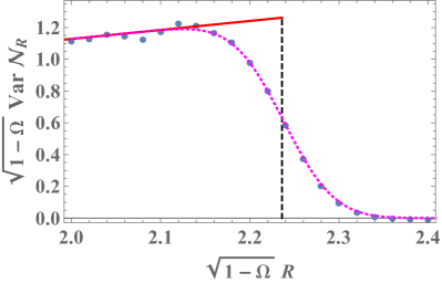
Figure 7: A zoom in on the vicinity of $R=R_{e}$ of the data plotted Fig. 6 (b) for $\Omega=0.99$ (blue circles), which is seen to be in excellent agreement with the magenta dotted line corresponding to the edge prediction (IV.2).

Although we have not attempted to compute exactly the higher cumulants of ${\cal N}_{R}$, we can give some general properties. The formula (48) extends to higher cumulants, which implies that all cumulants have the form of a piecewise linear function of $R$, namely

$$\left\langle{\cal N}_{R}^{2m}\right\rangle^{c}\simeq\sqrt{2}\ \,C_{k,2m}\,R\,\theta\left(\sqrt{\ell_{k}}<R<\sqrt{\ell_{k-1}}\right)$$ (56)

where the coefficients $C_{k,2m}$ can be obtained from the number cumulants for the standard $1d$ harmonic oscillator

$$C_{k,2m}=\int_{-\infty}^{+\infty}da\,\left.\left\langle{\cal N}_{(-\infty,a]}^{2m}\right\rangle^{c}\right|_{\frac{1}{2}u^{2},k}\;,$$ (57)

with $C_{k,2}=C_{k}$ given in Eqs. (51) and (52). They are discussed in Appendix F. Although we have not studied these coefficients in detail, we show, in section V that their large $k$ asymptotics match the $1-\Omega=O(1)$ result (21) in the limit $1-\Omega\ll 1$, as we also show explicitly in the case of the variance.

Finally, from the above predicted form of the cumulants, together with the relation (33), we conclude that the entanglement entropy should also be a piecewise linear function of $R$ in this regime. More precisely

$$S_{q}\left(D_{R}\right)\simeq\sqrt{2}\ \,\gamma_{q,k}\,R\,\theta\left(\sqrt{\ell_{k}}<R<\sqrt{\ell_{k-1}}\right)$$ (58)

where the prefactors $\gamma_{q,k}$’s are related to the bipartite entanglement entropy $S_{q}\left((-\infty,a],\frac{1}{2}u^{2},k\right)$ of the interval $(-\infty,a]$ for the standard $1d$ harmonic oscillator with Hamiltonian $-\frac{1}{2}\frac{\partial^{2}}{\partial u^{2}}+\frac{1}{2}u^{2}$ in its ground state with $k$ fermions, namely

$$\gamma_{q,k}=\int_{-\infty}^{+\infty}da\,S_{q}\left((-\infty,a],\frac{1}{2}u^{2},k\right)\;.$$ (59)

In the special case $k=1$, the entanglement entropy of a single fermion $S_{q}\left((-\infty,a],\frac{1}{2}u^{2},k\right)$ can be straightforwardly computed from the overlap matrix $A$ defined in (74), using that $S_{q}=\frac{1}{1-q}{\rm Tr}\log(A^{q}+(1-A)^{q})$, and yielding

$$S_{q}\left((-\infty,a],\frac{1}{2}u^{2},k=1\right)$$

$$\qquad=\frac{1}{1-q}\log\left(\frac{1}{2^{q}}{\rm erfc}(a)^{q}+\frac{1}{2^{q}}{\rm erfc}(-a)^{q}\right)\;,$$ (60)

which, together with Eqs. (58) and (59), coincides with the result obtained in LMG19 .

V Matching the two regimes in the bulk

It is now interesting to match (i) the result for the variance in (50), (51), which is valid in the vicinity of the LLL, i.e. for $1-\Omega\simeq c/N$ with $c=O(1)$ and $\mu=O(1)$, with (ii) the result in (18) which is valid in the limit $1-\Omega\ll 1$ and in the bulk of the Fermi gas. Let us consider now $1-\Omega\simeq c/N$ with $c\to+\infty$. Comparing Eqs. (38) and (41) we see that it also corresponds to large $\mu$, with $c\sim\mu^{2}/4$. We recall that $k$ varies from $k=0$ (at the edge of the Fermi gas) to $k=k_{\rm max}=n+1\simeq\mu/2$ near the center. Since we are interested in the bulk, $k=O(\mu)$ is large and we can use the estimate $k=\frac{\mu-(1-\Omega)\ell_{k}}{2}$. Using (50) and the asymptotic estimate (53) we obtain

$$\!\!\!\!{\rm Var}\,{\cal N}_{R}\simeq\mu\tilde{R}\frac{2}{\pi^{2}}\sqrt{1-2\left(1-\Omega\right)\tilde{R}^{2}}\times$$

$$\!\!\!\!\left[\log\mu+\log\left(1-\left(1-\Omega\right)2\tilde{R}^{2}\right)+5\log 2+\gamma_{E}-2\right].$$ (61)

where $\tilde{R}=R/\sqrt{2\mu}$ is fixed, and we have used $\ell_{k}\sim R^{2}$. On the other hand, one can consider Eq. (18) when $1-\Omega\ll 1$ and $R/R_{e}$ fixed, i.e., $\tilde{R}\sim R_{e}/\sqrt{2\mu}=1/\sqrt{1-\Omega^{2}}\gg 1$. As we show in the Appendix (120) in this limit the result matches precisely with Eq. (V).

Similarly, we can match the behavior of the higher cumulants in the two regimes. Although we did not calculate the constants $C_{k,2m}$ for $m\geq 2$, from Eq. (57) explicitly, we now find their large-$k$ behavior using a heuristic argument. At $k\gg 1$, the integrand in (57) takes a constant value in the bulk of the effective 1d fermi gas and vanishes outside the bulk UsCounting2020 for $m\geq 2$:

$$\left.\left\langle{\cal N}_{(-\infty,a]}^{2m}\right\rangle^{c}\right|_{\frac{1}{2}u^{2},k}\simeq\theta\left(\left|a\right|<\sqrt{2k}\right)\frac{\kappa_{2m}}{2}\,.$$ (62)

where $\kappa_{2m}$ is defined in Eq. (22), and the factor $1/2$ comes from the fact that it is a semi-infinite interval. Thus, Eq. (57) simply yields $C_{k,2m}\simeq\sqrt{2k}\,\kappa_{2m}$. As in the case of the variance, we now use $k=\frac{\mu-(1-\Omega)\ell_{k}}{2}$ which, together with (56), yields for $m\geq 2$

$$\left\langle{\cal N}_{R}^{2m}\right\rangle^{c}\simeq R\sqrt{2\mu-2(1-\Omega)R^{2}}\,\kappa_{2m}\,.$$ (63)

On the other hand, one can now take the limit $1-\Omega\ll 1$ in (21), and it is straightforward to see that the result is in perfect agreement with (63). Note that this heuristic argument can also be performed for the variance and reproduces the above results CkAsymptotic .

VI Extension to 3d geometry

We now consider the Hamiltonian (2). In cylindrical coordinates $(r,\phi,z)$, the eigenfunctions of $H$ are given by $\Psi\left(r,\phi,z\right)=\psi\left(r,\phi\right)\xi\left(z\right)$ where $\psi\left(r,\phi\right)$ are the eigenfunctions of the 2d Hamiltonian (4) and $\xi\left(z\right)$ are eigenfunctions of the $z$-component Hamiltonian, $H_{z}=\frac{p_{z}^{2}}{2}+U\left(z\right)$. or a system of $N$ noninteracting fermions in the ground state, one simply fills up the $N$ lowest single particle eigenstates.

Let ${\cal N}_{R}$ now be the number of particles in the cylinder $\left\{\left(r,\phi,z\right);\;r<R\right\}$ of radius $R$ around the origin, fully extended in the $z$ direction. Then one finds that the statistics of ${\cal N}_{R}$ decompose in the different sectors of $H_{z}$ in a manner similar to the angular decomposition described above in (9). In particular, the radial density, defined by

$$\rho_{\text{rad}}\left(r\right)=\int_{-\infty}^{\infty}\rho_{3d}\left(r,z\right)dz$$ (64)

where $\rho_{3d}\left(r,z\right)$ is the density of the 3d gas, is given by

$$\rho_{\text{rad}}\left(r\right)=\sum_{\epsilon_{z}}\rho_{2d}^{\left(\mu-\epsilon_{z}\right)}\left(r\right)$$ (65)

where $\rho_{2d}^{\left(\mu-\epsilon_{z}\right)}\left(r\right)$ is the density of an effective $2d$ fermi gas with single-particle Hamiltonian (4) and fermi energy $\mu-\epsilon_{z}$. Similarly, the variance of ${\cal N}_{R}$ is given by

$${\rm Var}\,{\cal N}_{R}=\sum_{\epsilon_{z}}{\rm Var}\,{\cal N}_{R,\left(2d\right)}^{\left(\mu-\epsilon_{z}\right)}$$ (66)

where ${\cal N}_{R,\left(2d\right)}^{\left(\mu-\epsilon_{z}\right)}$ is the number of particles in a circle of radius $R$ for a $2d$ fermi gas with single-particle Hamiltonian (4) and fermi energy $\mu-\epsilon_{z}$. These decompositions into the different sectors of $H_{z}$ extend to all higher cumulants as well, and therefore also to the entanglement entropy.

To illustrate these general results, let us consider an anisotropic harmonic oscillator described by $V(r)=r^{2}/2$ and $U(z)=\nu^{2}z^{2}/2$. Then Eq. (66) becomes

$${\rm Var}\,{\cal N}_{R}=\sum_{i_{z}=0}^{i_{\max}}{\rm Var}\,{\cal N}_{R,\left(2d\right)}^{\mu-\left(i_{z}+\frac{1}{2}\right)\nu}$$ (67)

with $i_{\max}=\text{Int}\left(\frac{\mu-1}{\nu}-\frac{1}{2}\right)$, and at $N\gg 1$, ${\rm Var}\,{\cal N}_{R,\left(2d\right)}^{\mu-\left(i_{z}+\frac{1}{2}\right)\nu}$ is given by (18) and/or by (50) [replacing $\mu\to\mu-\left(i_{z}+\frac{1}{2}\right)\nu$], depending on the scaling of $\Omega$ with $N$.

VII Conclusion

In summary, we studied the ground state of $N\gg 1$ noninteracting fermions in a two-dimensional harmonic trap of frequency $\omega$, in a reference frame which is rotating at angular frequency $\Omega<\omega$ around the origin. We calculated the FCS of the number of fermions ${\cal N}_{R}$ inside a disk of radius $R$ centered at the origin, within the bulk of the Fermi gas, i.e. for $R/R_{e}=O(1)$ where $R_{e}$ is the edge radius. We found rich and interesting behaviours in the two different scaling regimes: $\Omega/\omega=O(1)$ and $1-\Omega/\omega=O(1/N)$. In the latter regime we find that ${\rm Var}\,{\cal N}_{R}$ is given by a discontinuous piecewise linear function of $R$, of the form $\sim(R/R_{e})\sqrt{N}$. This behavior has the same origin as the “wedding cake” structure found for the density in KulkarniRotating2020 , namely the successive filling of Landau levels. We have shown how, upon decreasing $\Omega/\omega$, this piecewise linear function becomes a continuous function of $R$ with ${\rm Var}\,{\cal N}_{R}\sim\sqrt{N}\log N$ whose precise form we obtained analytically in the whole regime $\Omega/\omega=O(1)$. This prediction has also been tested numerically, see Fig. 6. We also studied the properties of the gas near the edge, and checked our results numerically, see Fig. 7. Similar results hold for higher cumulants, namely they are piecewise linear functions of $R$ in the regime $1-\Omega/\omega=O(1/N)$, while in the regime $\Omega/\omega=O(1)$ they are all proportional to a smooth function of $R$ obtained here. As an application, we also calculated the bipartite entanglement entropy of a disk of radius $R$ centered at the origin with the rest of the system. It exhibits a similar change of behavior as $\Omega$ is decreased, and in the regime $1-\Omega/\omega=O(1/N)$ we predict that it is also a piecewise linear function of $R$. Finally, we showed how the FCS can be studied in a three-dimensional extension of the model, where an additional confining potential is applied in the $z$ direction.

Another outcome of our results is that we obtain, by the same calculation, the FCS in $p$ space. Indeed the 2D Hamiltonian (1) is invariant by the transformation $H({\bf p},{\bf r})=H({\bf r},-{\bf p})$ which conserves the commutator. Hence the full kernel (not studied here) is the same in real space and in momentum space (in the LLL it is related to the kernel for the Ginibre ensemble). This implies that the momentum density has the same structure (at large $N$ uniform, with plateaus) as the one in real space, and that the cumulants are identical. This remark is of interest for time of flight experiments which measure the density in momentum space Pagano14 .

There are several avenues left for future research. A natural next step would be to calculate the coefficients $C_{k,2m}$ in (57) associated to the piecewise linear dependence of the higher cumulants in the regime $1-\Omega/\omega=O(1/N)$, and therefore, by virtue of (33), also obtain the exact coefficients $\gamma_{q,k}$ for the entanglement entropy, thus extending the results for $\gamma_{q,1}$ for the lowest Landau level in LMG19 . It would also be interesting to study the full distribution of ${\cal N}_{R}$, and in particular its large-deviation form, as was done in LaCroixGinibrePRE for the Ginibre ensemble (corresponding to $\Omega\to\omega$ in our system), see also Allez14 ; CharlierAnnuli in the context of Ginibre matrices.

Our results can be extended to more general trapping potentials $V(r)$. For $\Omega<\omega$ it is possible to apply the method developed in our previous work at $\Omega=0$ UsCounting2020 which was able to treat an arbitrary external potential. To explore further the regime $1-\frac{\Omega}{\omega}=O(1)$ one could consider a class of external potentials $V(r)$ which almost cancel the centrifugal potential, so that only a few Landau levels are occupied. One example was provided in KulkarniRotating2020 but there is a much larger class of potentials with similar features. In that case the FCS can still be obtained from the approximation by the $1d$ harmonic oscillator used in the present work. As a consequence our results should exhibit universal features for this larger class of potentials. Another interesting example is a potential $V(r)$ that contains anharmonic terms, in addition to a harmonic term: one could consider the case $\Omega/\omega>1$ where the effective radial potential can become a double well. In such situations it is known that the FCS is anomalous near the transition to the double well, see smi20 for an example in $1d$.

Additional important extensions of our results would be (i) to systems of interacting fermions, as was recently done for some particular 1d systems InteractingFCS , and (ii) to nonzero temperature, where one could use the framework of DeanPLDReview . These extensions could be very useful towards a theory that describes more accurately systems studied in experiments.

Acknowledgments: We thank M. Kulkarni and B. Lacroix-A-Chez-Toine for previous collaborations on related topics. NRS acknowledges support from the Yad Hanadiv fund (Rothschild fellowship). This research was supported by ANR grant ANR-17-CE30-0027-01 RaMaTraF.

Appendix A Semi-classical density

From general results, the Wigner function in the bulk and for large $N$ is given by the semi-classical formula Wigner18

$$W({\bf r},{\bf p})\simeq\frac{1}{(2\pi)^{2}}\theta\left(\mu-\frac{1}{2}\left({\bf p}-\Omega\,\hat{{\bf z}}\wedge{\bf r}\right)^{2}-V(r)+\frac{\Omega^{2}}{2}r^{2}\right)\;,$$ (68)

where $\theta(z)$ is the Heaviside step function and $\hat{\bf z}$ is the unit vector along the $z$ axis. The mean density can be obtained from this formula using $\rho({\bf r})=\int d^{2}{\bf p}\,W({\bf r},{\bf p})$.

In the case of the harmonic potential $V(r)=\frac{1}{2}r^{2}$, this yields

$$\rho({\bf r})\simeq\frac{1}{(2\pi)^{2}}\int d^{2}{\bf p}\,\theta\left(\mu-\frac{1}{2}({\bf p}-\Omega\,\hat{{\bf z}}\wedge{\bf r})^{2}-\frac{(1-\Omega^{2})}{2}r^{2}\right)=\frac{1}{(2\pi)^{2}}\int d^{2}{\bf p}\,\theta\left(\mu-\frac{1}{2}{\bf p}^{2}-\frac{(1-\Omega^{2})}{2}r^{2}\right)=\frac{k_{F}(r)^{2}}{4\pi}\,,$$

(69)

$$k_{F}(r)=\sqrt{2\mu-(1-\Omega^{2})r^{2}}$$ (70)

obtained upon shifting the ${\bf p}$ variable. We have introduced the local 2D Fermi momentum $k_{F}(r)$. These results are given in the main text in Eq. (13). The total number of particles is

$$N=\int\rho\left({\bf r}\right)d^{2}{\bf r}\simeq\frac{1}{4\pi}\int d^{2}{\bf r}\left[2\mu-\left(1-\Omega^{2}\right)r^{2}\right]=\frac{\mu^{2}}{2\left(1-\Omega^{2}\right)}$$ (71)

in agreement with (12) which was obtained in the main text using a different method.

Note that the mean density in momentum space, $\hat{\rho}({\bf p})$, has a very similar form. Indeed, by rearranging the terms we obtain

$$\hat{\rho}({\bf p})\simeq\frac{1}{(2\pi)^{2}}\int d^{2}{\bf r}\,\theta\left(\mu-\frac{1}{2}(x-\Omega p_{y})^{2}-\frac{1}{2}(y+\Omega p_{x})^{2}-\frac{(1-\Omega^{2})}{2}r^{2}\right)=\frac{2\mu-(1-\Omega^{2})p^{2}}{4\pi}\;.$$ (72)

Remark. Note that in the quite different limit of the LLL, i.e. $\Omega\to 1$, the kernel at large $N$ and in the bulk is given by the kernel of the Ginibre ensemble of random matrix theory, namely $K(z,z^{\prime})=\frac{1}{\pi}e^{-\frac{1}{2}|z|^{2}-\frac{1}{2}|z^{\prime}|^{2}+z(z^{\prime})^{*}}$ with $z=x+iy$. One can check, by simple Fourier transform, that in $p$ space it retains a similar form than in real space. This, as well as the fact that (72) and (A) are very similar, are two manifestation of the symmetry $H({\bf p},{\bf r})=H({\bf r},-{\bf p})$ of the Hamiltonian, as discussed in the conclusion of this paper. This shows that correlations in real and momentum space have identical forms (which is an exact property valid for any $N$).

Appendix B FCS for the equivalent harmonic oscillator problem

In this section we compute the coefficients $C_{k}$ defined in the text. Consider the eigenfunction $\varphi_{j}$’s of the harmonic oscillator $H=\frac{p^{2}}{2}+\frac{x^{2}}{2}$

$$\varphi_{j}(x)=\frac{1}{\sqrt{\sqrt{\pi}\,2^{j}j!}}H_{j}(x)e^{-x^{2}/2}\quad,\quad j=0,1,\dots$$ (73)

One defines the overlap matrix and its complementary

$$A_{ij}(a)=\int_{-\infty}^{a}dx\,\varphi_{i}(x)\varphi_{j}(x)\quad,\quad\delta_{ij}-A_{ij}(a)=\int_{a}^{+\infty}dx\,\varphi_{i}(x)\varphi_{j}(x)\;.$$ (74)

We aim to calculate the integrated variance when the oscillator is occupied up to level $j=n$, which corresponds to $m_{\ell}=n+1$ fermions and to the coefficient $C_{k=n+1}$ defined in the text. Using the standard formula which relates the variance to the overlap matrix (see e.g. CMV2012 ) we have

$$C_{n+1}=B_{n}=\int_{-\infty}^{\infty}da\sum_{i,j=0}^{n}A_{ij}(a)(\delta_{ij}-A_{ij}(a))$$ (75)

where we have defined $B_{n}=C_{n+1}$ for convenience. We first calculate the generating function

$$\tilde{B}(z,t)=\int_{-\infty}^{\infty}da\sum_{i,j\geq 0}z^{i}t^{j}A_{ij}(a)(\delta_{ij}-A_{ij}(a))=\sum_{i,j\geq 0}z^{i}t^{j}\int_{-\infty}^{\infty}da\int_{-\infty}^{a}dx\,\varphi_{i}(x)\varphi_{j}(x)\int_{a}^{+\infty}dy\,\varphi_{i}(y)\varphi_{j}(y)\;.$$ (76)

Using the Mehler formula

$$\sum_{j=0}^{\infty}\frac{z^{j}}{2^{j}j!}H_{j}(x)H_{j}(y)=G(x,y,z)=\frac{1}{\sqrt{1-z^{2}}}e^{\frac{2xyz-(x^{2}+y^{2})z^{2}}{1-z^{2}}}\;,$$ (77)

the generating function can be written as

$$\tilde{B}(z,t)=\frac{1}{\pi}\int_{-\infty}^{\infty}da\int_{-\infty}^{a}dx\int_{a}^{+\infty}dy\,G(x,y,z)G(x,y,t)e^{-x^{2}-y^{2}}\;.$$ (78)

To perform this integral we shift the arguments $x,y$ by defining $x=a-X$ and $y=a+Y$, where now $X,Y$ are both integrated on $[0,+\infty[$. The integral over $a$ is an elementary Gaussian integral and leads to a simple Gaussian integrand depending only on $X+Y$. Its integration is elementary and leads to

$$\tilde{B}(z,t)=\frac{1}{\sqrt{2\pi}}\frac{\sqrt{1-t}\sqrt{1-z}}{(1-tz)^{3/2}}$$ (79)

From this result we obtain the generating function for the $B_{k}$ as follows. Define

$$B(z,t)=\sum_{n_{1},n_{2}\geq 0}z^{n_{1}}t^{n_{2}}\sum_{i=0}^{n_{1}}\sum_{j=0}^{n_{2}}\int_{-\infty}^{\infty}daA_{ij}(a)(\delta_{ij}-A_{ij}(a))$$ (80)

which is such that the $B_{n}$’s are the diagonal coefficients for $n_{1}=n_{2}$

$$B_{n}=B(z,t)|_{z^{n}t^{n}}\quad,\quad[B(z,t)]_{\rm diag}=\sum_{n\geq 0}(zt)^{n}B_{n}$$ (81)

On the other hand one has simply

$$B(z,t)=\frac{1}{1-z}\frac{1}{1-t}\tilde{B}(z,t)=\frac{1}{\sqrt{2\pi}}\frac{1}{\sqrt{1-t}\sqrt{1-z}(1-tz)^{3/2}}\;.$$ (82)

The diagonal part of $B(z,t)$ can be extracted as follows. Using that $(1+x)^{a}=\sum_{n\geq 0}{\rm Bin}(a,n)x^{n}$ where here we denote ${\rm Bin}(a,n)=\frac{\Gamma(a+1)}{\Gamma(n+1)\Gamma(a-n+1)}$ the binomial coefficient, one has

$$\left[(1-z)^{-1/2}(1-t)^{-1/2}\right]_{{\rm diag}}=\sum_{n\geq 0}B\left(-\frac{1}{2},n\right)^{2}(zt)^{n}=\,_{2}F_{1}\left(\frac{1}{2},\frac{1}{2},1,zt\right)=\frac{2K(\sqrt{zt})}{\pi}$$ (83)

where $K\left(x\right)=\frac{\pi}{2}\sum_{n=0}^{\infty}\left[\frac{\left(2n-1\right)!!}{\left(2n\right)!!}\right]^{2}x^{2n}$ is the elliptic integral of the first kind. This leads to (with $*$ denoting the convolution)

$$B_{n}=\frac{(-1)^{n}}{\sqrt{2\pi}}B\left(-\frac{3}{2},n\right)*B\left(-\frac{1}{2},n\right)^{2}=\frac{1}{\sqrt{2\pi}}\sum_{k=0}^{n}(-1)^{n-k}B\left(-\frac{3}{2},n-k\right)B\left(-\frac{1}{2},k\right)^{2}$$ (84)

This formula gives, for $n=0,1,\dots$

$$B_{n}={\frac{1}{\sqrt{2\pi}}}\left\{1,\frac{7}{4},\frac{153}{64},\frac{759}{256},\frac{57225}{16384},\frac{261207}{65536},\frac{4667201}{1048576},\frac{20525111}{4194304},\frac{5709117897}{1073741824},\frac{24584746575}{4294967296},\frac{420344955129}{68719476736},\dots\right\}$$ (85)

The corresponding numerical values are

$$B_{n}=\frac{1}{\sqrt{2\pi}}\{1,1.75,2.39063,2.96484,3.49274,3.9857,4.45099,4.89357,5.31703,5.72408,6.11682\}$$ (86)

Another way to present the result is in the form of the generating function

$$B(z)=\sum_{n\geq 0}z^{n}B_{n}={\frac{1}{\sqrt{2\pi}}}\,_{2}F_{1}\left(\frac{1}{2},\frac{1}{2},1,z\right)(1-z)^{-3/2}$$ (87)

To extract a more compact formula for the $B_{n}$ and the $C_{k}=B_{k-1}$ given in the text in (51), we will use a slightly different method. Starting from (82) we use an integral represention

$$B(z,t)=\frac{1}{\sqrt{2\pi}}\frac{1}{\sqrt{1-t}\sqrt{1-z}(1-tz)^{3/2}}=\frac{1}{\sqrt{2\pi}}\frac{2}{\pi^{3/2}}\int_{0}^{+\infty}dx_{1}dx_{2}dx_{3}x_{1}^{-1/2}x_{2}^{-1/2}x_{3}^{1/2}e^{-x_{1}(1-t)-x_{2}(1-z)-x_{3}(1-zt)}$$

$$=\frac{1}{\sqrt{2\pi}}\frac{2}{\pi^{3/2}}\sum_{n_{1},n_{2},n_{3}\geq 0}\frac{\Gamma(n_{1}+\frac{1}{2})\Gamma(n_{2}+\frac{1}{2})\Gamma(n_{3}+\frac{3}{2})}{n_{1}!n_{2}!n_{3}!}z^{n_{1}+n_{3}}t^{n_{2}+n_{3}}$$ (88)

$$=\frac{1}{\sqrt{2\pi}}\frac{2}{\pi^{3/2}}\sum_{n_{1},n_{2}\geq 0}z^{n_{1}}t^{n_{2}}\sum_{n_{3}=0}^{\min(n_{1},n_{2})}\frac{\Gamma(n_{1}-n_{3}+\frac{1}{2})\Gamma(n_{2}-n_{3}+\frac{1}{2})\Gamma(n_{3}+\frac{3}{2})}{(n_{1}-n_{3})!(n_{2}-n_{3})!n_{3}!}$$ (89)

where in the second line we have expanded the exponentials in powers of $z$ and $t$ and integrated over the auxiliary variables $x_{i}$ and in the third line we have rearranged the terms. The diagonal term $n_{1}=n_{2}$ in the double series provides the expression for $B_{n}$

$$B_{n}=\frac{1}{\sqrt{2\pi}}\frac{2}{\pi^{3/2}}\sum_{n_{3}=0}^{n}\frac{\Gamma(n-n_{3}+\frac{1}{2})^{2}\Gamma(n_{3}+\frac{3}{2})}{[(n-n_{3})!]^{2}n_{3}!}$$ (90)

Using mathematica this sum can be performed and leads to

$$C_{n+1}=B_{n}=\frac{1}{\sqrt{2\pi}}\frac{\Gamma\left(n+\frac{1}{2}\right)^{2}\,_{3}F_{2}\left(\frac{3}{2},-n,-n;\frac{1}{2}-n,\frac{1}{2}-n;1\right)}{\pi n!^{2}}$$ (91)

which leads to the result (51) given in the text for $C_{k}$.

Let us now study the asymptotic behavior of $C_{k}$ for large $k$. It can be obtained from the behavior of the generating function $B(z)$ in Eq. (87) for $z\to 1$. In that limit one finds

$$B(z)\simeq\frac{1}{\sqrt{2}\,\pi^{3/2}}\frac{1}{(1-z)^{3/2}}\left[-\log(1-z)+4\log 2\right]\;.$$ (92)

By setting $z=e^{-s}$ one obtains

$$B_{n}\simeq\frac{\sqrt{2}}{\pi^{2}}\sqrt{n}(\log n+b)\quad,\quad b=6\log 2+\gamma-2\;,$$ (93)

which gives the result (53) mentioned in the text for $C_{k}$. To obtain this result (93), we used the relation

$$\sum_{n}z^{n}\sqrt{n}\left(\log n+c\right)\simeq\int_{0}^{+\infty}dn\,e^{-sn}\sqrt{n}\left(\log n+c\right)=\frac{\sqrt{\pi}}{2s^{3/2}}\left(-\log s-2\log 2-\gamma+2+c\right)\;.$$ (94)

Appendix C Density and variance near the steps $R\simeq\sqrt{\ell_{k}}$

C.1 The step structure in the density

Here we calculate the structure of the step, recovering the results of KulkarniRotating2020 by a different method. In KulkarniRotating2020 the result was obtained by first writing the exact formula for the density in the exact eigenfunctions, in terms of the Laguerre polynomials and in a second stage taking the large $\mu$ limit and using standard asymptotic formulas for the Laguerre polynomials in terms of Hermite polynomials. Here we use, more directly, that at large $\mu$ the problem can be mapped to a harmonic oscillator. This also provides a test of the approach in the text.

Starting from (44) in the main text, we zoom in around the step by assuming that $r\simeq\sqrt{\ell_{k}}$ for some $k$. Thus, in the sum in Eq. (44) only the terms with $k$ and $k+1$ contribute,

$$2\pi r\rho\left(r\right)\simeq\int_{\ell_{k}}^{\ell_{k-1}}d\ell\,\rho_{1d\text{HO},k}\left(r-\sqrt{\ell}\right)+\int_{\ell_{k+1}}^{\ell_{k}}d\ell\,\rho_{1d\text{HO},k+1}\left(r-\sqrt{\ell}\right)\,.$$ (95)

Adding and subtracting the term $\int_{\ell_{k+1}}^{\ell_{k}}d\ell\,\rho_{1d\text{HO},k}\left(r-\sqrt{\ell}\right)$ to the r.h.s. of the last equation, one obtains $2\pi r\rho\left(r\right)\simeq I_{1}+I_{2}$ where

$$I_{1}=\int_{\ell_{k+1}}^{\ell_{k-1}}d\ell\,\rho_{1d\text{HO},k}\left(r-\sqrt{\ell}\right)\simeq 2kr$$ (96)

[the last approximate equality is obtained using the same approximation as in Eqs. (45) and (46)] and

$$I_{2}=\int_{\ell_{k+1}}^{\ell_{k}}\left[\rho_{1d\text{HO},k+1}\left(r-\sqrt{\ell}\right)-\rho_{1d\text{HO},k}\left(r-\sqrt{\ell}\right)\right]d\ell\,.$$ (97)

In order to calculate $I_{2}$, we now (i) change variables $\sqrt{\ell}=r-u$ where we assume $u\ll r$ so $d\ell=2\left(u-r\right)du\simeq-2rdu$ [this is the same change of variables that is described below (46)] and (ii) recall that

$$\rho_{1d\text{HO},k}\left(u\right)=\sum_{i=0}^{k-1}\left|\psi_{i}\left(u\right)\right|^{2}$$ (98)

where $\psi_{i}(x)$ is the eigenfunction function associated to the $i^{\text{th}}$ energy level of the 1d harmonic oscillator $H_{\rm 1D\text{HO}}=-\frac{1}{2}\partial_{u}^{2}+2u^{2}$. Putting it all together we find

$$I_{2}\simeq 2r\int_{r-\sqrt{\ell_{k}}}^{r-\sqrt{\ell_{k+1}}}\left|\psi_{k}\left(u\right)\right|^{2}du\,.$$ (99)

Now using

$$\psi_{k}\left(u\right)=\left(\frac{\sqrt{2}}{\sqrt{\pi}2^{k}k!}\right)^{1/2}e^{-u^{2}}H_{k}(\sqrt{2}u)$$ (100)

where $H_{k}(x)$ is the Hermite polynomial of degree $k$, and replacing the upper limit of the integral (99) by infinity (which is a good approximation due to the assumption $r\simeq\sqrt{\ell_{k}}$) we obtain the density around the step i.e. for $r-\sqrt{\ell_{k}}=O(1)$

$$\rho\left(r\right)\simeq\frac{k}{\pi}+f_{k}^{\text{edge}}\left(\sqrt{2}(\sqrt{\ell_{k}}-r)\right),\qquad f_{k}^{\text{edge}}\left(x\right)=\frac{1}{\pi^{3/2}2^{k}k!}\int_{-x}^{\infty}e^{-v^{2}}\left[H_{k}(v)\right]^{2}dv,$$ (101)

in perfect agreement with KulkarniRotating2020 (see also Dunne94 ; HH2013 ; FL20 ).

C.2 The step structure in the variance

We begin from the first line in Eq. (48), and assume that $R\simeq\sqrt{\ell_{k}}$ for some $k$. Again we zoom in around the step by assuming that only the terms with occupation numbers $k$ and $k+1$ have a non-negligible contribution to (48)

$${\rm Var}\,{\cal N}_{R}\simeq\int_{\ell_{k}}^{\ell_{k-1}}d\ell\,{\rm Var}\,\left.{\cal N}_{\left[-\sqrt{\ell},R-\sqrt{\ell}\right]}\right|_{2u^{2},k}+\int_{\ell_{k+1}}^{\ell_{k}}d\ell\,{\rm Var}\,\left.{\cal N}_{\left[-\sqrt{\ell},R-\sqrt{\ell}\right]}\right|_{2u^{2},k+1}\,.$$ (102)

Adding and subtracting $\int_{\ell_{k+1}}^{\ell_{k}}d\ell\,{\rm Var}\,\left.{\cal N}_{\left[-\sqrt{\ell},R-\sqrt{\ell}\right]}\right|_{2u^{2},k}$ to the r.h.s. and performing the change of variable $a=R-\sqrt{\ell}$, we find

$${\rm Var}\,{\cal N}_{R}\simeq\sqrt{2}C_{k}R+2R\int_{R-\sqrt{\ell_{k}}}^{\infty}da\,\left({\rm Var}\,\left.{\cal N}_{\left(-\infty,\sqrt{2}a\right]}\right|_{\frac{1}{2}u^{2},k+1}-{\rm Var}\,\left.{\cal N}_{\left(-\infty,\sqrt{2}a\right]}\right|_{\frac{1}{2}u^{2},k}\right)$$ (103)

where the first term was obtained using the same calculations as those that give Eq. (50) in the main text, and we used Eq. (49). Note that the upper bound $R-\sqrt{\ell_{k+1}}$ in (103) can be safely set to infinity. We now use the known expression for the number variance in determinantal point processes MehtaBook ; Forrester

$${\rm Var}\,\left.{\cal N}_{\left(-\infty,\sqrt{2}a\right]}\right|_{\frac{1}{2}u^{2},k}=\int_{-\infty}^{\sqrt{2}a}dx\int_{\sqrt{2}a}^{\infty}dy\,K_{k}\left(x,y\right)^{2}$$ (104)

where

$$K_{k}\left(x,y\right)=\sum_{i=0}^{k-1}\varphi_{i}\left(x\right)\varphi_{i}\left(y\right)$$ (105)

is the kernel in terms of the eigenfunctions $\varphi_{k}(x)$ of the harmonic oscillator defined in Eq. (73). Thus

$$K_{k+1}\left(x,y\right)^{2}=\left[K_{k}\left(x,y\right)+\varphi_{k}\left(x\right)\varphi_{k}\left(y\right)\right]^{2}=K_{k}\left(x,y\right)^{2}+2\varphi_{k}\left(x\right)\varphi_{k}\left(y\right)K_{k}\left(x,y\right)+\varphi_{k}^{2}\left(x\right)\varphi_{k}^{2}\left(y\right)$$ (106)

leading to

$${\rm Var}\,\left.{\cal N}_{\left(-\infty,\sqrt{2}a\right]}\right|_{\frac{1}{2}u^{2},k+1}-{\rm Var}\,\left.{\cal N}_{\left(-\infty,\sqrt{2}a\right]}\right|_{\frac{1}{2}u^{2},k}=\int_{-\infty}^{\sqrt{2}a}dx\int_{\sqrt{2}a}^{\infty}dy\,\left[2\varphi_{k}\left(x\right)\varphi_{k}\left(y\right)K_{k}\left(x,y\right)+\varphi_{k}^{2}\left(x\right)\varphi_{k}^{2}\left(y\right)\right]$$

$$\qquad\qquad\qquad\qquad\qquad\qquad\qquad\qquad\qquad=\int_{-\infty}^{\sqrt{2}a}dx\int_{\sqrt{2}a}^{\infty}dy\,2\varphi_{k}\left(x\right)\varphi_{k}\left(y\right)K_{k}\left(x,y\right)+A_{k}\left(\sqrt{2}a\right)\left[1-A_{k}\left(\sqrt{2}a\right)\right]\,,$$

where $A_{k}\left(v\right)=A_{kk}\left(v\right)=\int_{-\infty}^{v}\varphi_{k}^{2}\left(x\right)dx$ and we used the normalization $\int_{-\infty}^{\infty}\varphi_{k}^{2}\left(x\right)dx=1$. The remaining integral is

$$\int_{-\infty}^{\sqrt{2}a}dx\int_{\sqrt{2}a}^{\infty}dy\,2\varphi_{k}\left(x\right)\varphi_{k}\left(y\right)K_{k}\left(x,y\right)=2\sum_{i=0}^{k-1}\int_{-\infty}^{\sqrt{2}a}\varphi_{i}\left(x\right)\varphi_{k}\left(x\right)dx\int_{\sqrt{2}a}^{\infty}\varphi_{k}\left(y\right)\varphi_{i}\left(y\right)dy=-2\sum_{i=0}^{k-1}A_{ik}\left(\sqrt{2}a\right)^{2}$$ (108)

where we recall the definition of the overlap matrix

$$A_{ik}\left(v\right)=\int_{-\infty}^{v}\varphi_{i}\left(x\right)\varphi_{k}\left(x\right)dx$$ (109)

and we used the orthogonality $\int_{-\infty}^{\infty}\varphi_{i}\left(x\right)\varphi_{k}\left(x\right)dx=0$, $i\neq k$. These equations together lead to Eq. (54) in the main text with the scaling function

$$f_{k}^{\text{edge},\text{Var}}\left(s\right)=\int_{s}^{+\infty}dv\,\left\{-2\sum_{i=0}^{k-1}A_{ik}\left(v\right)^{2}+A_{k}\left(v\right)\left[1-A_{k}\left(v\right)\right]\right\}.$$ (110)

In particular, $f_{k}^{\text{edge},\text{Var}}\left(s\to+\infty\right)=0$ [because $A_{k}\left(v\to\infty\right)=1$ and $A_{ik}\left(v\to\infty\right)=0$], matching smoothly with (50). Note also that for $f_{k}^{\text{edge},\text{Var}}\left(s\to-\infty\right)=C_{k+1}-C_{k}$ as can be checked by comparing with the definition of $C_{k}$ in (75).

Appendix D Simplifying $B_{\tilde{R},\Omega}$ and taking the limit $1-\Omega\ll 1$

We begin by rewriting Eq. (III.1) by expanding the logarithmic term and then performing the integral over the $\lambda$-independent terms:

$$B_{\tilde{R},\Omega} = \int_{\lambda_{-}(\tilde{R})}^{\lambda_{+}(\tilde{R})}\frac{d\lambda}{2\pi^{2}}\left[\log\left(4\tilde{R}\frac{(1-(\tilde{R}^{2}+\frac{\lambda^{2}}{4\tilde{R}^{2}}-\Omega\lambda))_{+}^{\frac{3}{2}}}{((1+\Omega\lambda)^{2}-\lambda^{2})_{+}^{\frac{1}{2}}}\right)+c_{2}\right]=\frac{1}{2\pi^{2}}\left(\lambda_{+}-\lambda_{-}\right)\left[c_{2}+\log\left(4\tilde{R}\right)\right]$$ (111)

$$+ \frac{3}{2}\frac{1}{2\pi^{2}}\int_{\lambda_{-}}^{\lambda_{+}}d\lambda\log\left(1-\left(\tilde{R}^{2}+\frac{\lambda^{2}}{4\tilde{R}^{2}}-\Omega\lambda\right)\right)-\frac{1}{2}\frac{1}{2\pi^{2}}\int_{\lambda_{-}}^{\lambda_{+}}d\lambda\log\left((1+\Omega\lambda)^{2}-\lambda^{2}\right)\,.$$

The two remaining integrals can in fact be calculated explicitly. The first one gives a simple result:

$$\int_{\lambda_{-}}^{\lambda_{+}}d\lambda\log\left(1-\left(\tilde{R}^{2}+\frac{\lambda^{2}}{4\tilde{R}^{2}}-\Omega\lambda\right)\right) = \int_{\lambda_{-}}^{\lambda_{+}}d\lambda\log\left(\frac{1}{4\tilde{R}^{2}}\left(\lambda_{+}-\lambda\right)\left(\lambda-\lambda_{-}\right)\right)$$ (112)

$$= 2\left(\lambda_{+}-\lambda_{-}\right)\left[\log\left(\lambda_{+}-\lambda_{-}\right)-1-\log\left(2\tilde{R}\right)\right]\,,$$

but the second one gives a result that is rather cumbersome:

$$\int_{\lambda_{-}}^{\lambda_{+}}d\lambda\log\left((1+\Omega\lambda)^{2}-\lambda^{2}\right)=\left[\lambda\left(\log\left((\lambda\Omega+1)^{2}-\lambda^{2}\right)-2\right)+\frac{\log(\lambda(\Omega-1)+1)}{\Omega-1}+\frac{\log(\lambda\Omega+\lambda+1)}{\Omega+1}\right]_{\lambda_{-}}^{\lambda_{+}}\,.$$ (113)

So, using $A_{\tilde{R},\Omega}=\frac{1}{2\pi^{2}}\left(\lambda_{+}-\lambda_{-}\right)$ we reach

$$B_{\tilde{R},\Omega}=A_{\tilde{R},\Omega}\left[c_{2}+\log 2+3\log\left(\lambda_{+}-\lambda_{-}\right)-3-2\log\left(2\tilde{R}\right)\right]-\frac{1}{2}\frac{1}{2\pi^{2}}\int_{\lambda_{-}}^{\lambda_{+}}d\lambda\log\left((1+\Omega\lambda)^{2}-\lambda^{2}\right)\;.$$ (114)

Now we consider the limit $1-\Omega\ll 1$ with $\tilde{R}\sim\left(1-\Omega\right)^{-1/2}\gg 1$. In this limit, one has $\lambda_{+}\simeq\lambda_{-}\simeq 2\tilde{R}^{2}\gg 1$, and it is convenient to calculate the integral (113) approximately. Neglecting terms $O(1)$ or smaller, the term that is inside the logarithm in the integrand in (113) is (using $\lambda\simeq 2\tilde{R}^{2}\gg 1$)

$$(1+\Omega\lambda)^{2}-\lambda^{2}\simeq 2\lambda\left[1-\left(1-\Omega\right)\lambda\right]\simeq 4\tilde{R}^{2}\left[1-2\left(1-\Omega\right)\tilde{R}^{2}\right].$$ (115)

Under this approximation the integration is trivial because the integrand is a constant:

$$\int_{\lambda_{-}}^{\lambda_{+}}d\lambda\log\left((1+\Omega\lambda)^{2}-\lambda^{2}\right)\simeq\left(\lambda_{+}-\lambda_{-}\right)\left[2\log\left(2\tilde{R}\right)+\log\left(1-2\left(1-\Omega\right)\tilde{R}^{2}\right)\right].$$ (116)

Plugging this into (114) yields

$$B_{\tilde{R},\Omega} \simeq A_{\tilde{R},\Omega}\left[3\log\left(\frac{\lambda_{+}-\lambda_{-}}{2\tilde{R}}\right)-\frac{1}{2}\log\left(1-2\left(1-\Omega\right)\tilde{R}^{2}\right)+c_{2}+\log 2-3\right]$$ (117)

$$\simeq A_{\tilde{R},\Omega}\left[\log\left(1-2(1-\Omega)\tilde{R}^{2}\right)+c_{2}+4\log 2-3\right]$$

Finally, using

$$A_{\tilde{R},\Omega}=\frac{2}{\pi^{2}}\tilde{R}\sqrt{1-(1-\Omega^{2})\tilde{R}^{2}}\underbrace{\simeq}_{1-\Omega\ll 1}\frac{2}{\pi^{2}}\tilde{R}\sqrt{1-2(1-\Omega)\tilde{R}^{2}}$$ (118)

we get

$$B_{\tilde{R},\Omega}\simeq\frac{2}{\pi^{2}}\tilde{R}\sqrt{1-2(1-\Omega)\tilde{R}^{2}}\left[\log\left(1-2(1-\Omega)\tilde{R}^{2}\right)+c_{2}+4\log 2-3\right]\;.$$ (119)

Plugging Eqs. (118) and (119) into (18), we reach

$${\rm Var}\,{\cal N}_{R}\simeq\frac{2}{\pi^{2}}\tilde{R}\sqrt{1-2(1-\Omega)\tilde{R}^{2}}\mu\left[\log\mu+\log\left(1-2(1-\Omega)\tilde{R}^{2}\right)+c_{2}+4\log 2-3\right]$$ (120)

which agrees with (V).

Appendix E Details of numerical simulations

Here we briefly describe the method that we used in order to simulate the radial coordinates $r_{1},\dots,r_{N}$ of the particles for the rotating HO in 2d, which we then used in order to empirically measure the densities and number variances displayed in Figs. 3 and 6 in the main text. We use the decoupling between angular sectors, see UsCounting2020 for details, so that we generate samples of radial coordinates within each angular sector $\ell$ independently. For each sector we generate samples of the positions of $m_{\ell}$ fermions in the effective 1d potential $V_{\ell}(r)=\frac{r^{2}}{2}+\frac{\ell^{2}-\frac{1}{4}}{2r^{2}}-\Omega\ell$ [which is simply (5) for the HO], where $m_{\ell}$ is given by (7). This is conveniently done by exploiting the mapping between the effective 1d systems to the eigenvalues of a random matrix from the Wishart-Laguerre Unitary Ensemble (LUE) – this mapping is described, e.g., in the recent review DeanReview2019 . Finally, we used the tridiagonal matrix representations of Gaussian unitary ensemble (GUE) and LUE matrices (Dumitriu2002, ) in order to efficiently generate their eigenvalues. The code that we used is avaliable in SM .

Appendix F Higher cumulants

Here we sketch how one would proceed to compute the higher cumulants of ${\cal N}_{R}$. Ideally we would like to obtain the FCS generating function. By the same arguments as in the main text it will be a piecewise linear function of $R$. In the interval in $\sqrt{\ell_{k}}<R<\sqrt{\ell_{k-1}}$ associated to the Landau level indexed by $n=k-1$

$$\log\left\langle e^{-s\left({\cal N}_{R}-\left\langle{\cal N}_{R}\right\rangle\right)}\right\rangle \simeq \sqrt{2}R\int_{-\infty}^{\infty}da\log\left\langle e^{-s\left({\cal N}_{\left(-\infty,a\right]}-\left\langle{\cal N}_{\left(-\infty,a\right]}\right\rangle\right)}\right\rangle$$ (121)

$$= \sqrt{2}R\int_{-\infty}^{\infty}da\left(\log\det\left[\delta_{ij}-\left(1-e^{-s}\right)A_{ij}(a)\right]+s\,{\rm Tr}A(a)\right)$$

where ${\cal N}_{\left(-\infty,a\right]}$ is the number of fermions in $\left(-\infty,a\right]$ for the standard harmonic oscillator (HO) $H=\frac{p^{2}}{2}+\frac{x^{2}}{2}$, and the trace and determinant are over the eigenstates $i,j=0,\dots,n$ of the HO. Note that we had to substract the mean, since $\int da\left\langle{\cal N}_{\left(-\infty,a\right]}\right\rangle=+\infty$ (a manifestation of the fact that all cumulants are piecewise linear in $R$, except the mean which has a quadratic dependence $R^{2}$). In the second line we have used the standard formula for the FCS of a determinantal process. The overlap matrix $A_{ij}(a)$ is defined in (74). Computing the integrals and expanding (121) in powers of $s$ allows to obtain the $p$-th cumulant as the coefficient of $s^{p}/p!$.

Let us give some examples of this method. One has for $n=k-1=0$

$$\frac{1}{\sqrt{2}R}\log\left\langle e^{-s\left({\cal N}_{R}-\left\langle{\cal N}_{R}\right\rangle\right)}\right\rangle\simeq\int_{-\infty}^{\infty}da\left[\log\left(1-\frac{1-e^{-s}}{2}\left(1+{\rm erf}(a)\right)\right)+\frac{s}{2}\left(1+{\rm erf}(a)\right)\right]$$ (122)

$$=\frac{s^{2}}{2}\frac{1}{\sqrt{2\pi}}+\frac{s^{4}}{4!}\int_{-\infty}^{\infty}\frac{-3\text{erf}(a)^{4}+4\text{erf}(a)^{2}-1}{8}\,da+\frac{s^{6}}{6!}\int_{-\infty}^{\infty}\frac{-15\text{erf}(a)^{6}+30\text{erf}(a)^{4}-17\text{erf}(a)^{2}+2}{8}\,da+O(s^{8})$$

$$=\frac{s^{2}}{2}\frac{1}{\sqrt{2\pi}}+\left[\frac{9\sqrt{2}}{\pi^{3/2}}\text{arctan}\left(\frac{1}{\sqrt{8}}\right)-\sqrt{\frac{2}{\pi}}\right]\frac{s^{4}}{4!}+0.00893625\frac{s^{6}}{6!}+O(s^{8})$$ (123)

which is in agreement with the results for the first three cumulants of LMG19 . We calculated the fourth cumulant as follows. We rewrite the coefficient of $s^{4}/4!$ as $(4I_{2}-3I_{4})/8$ where we defined $I_{m}=\int_{-\infty}^{\infty}\left(\text{erf}\left(x\right)^{m}-1\right)dx$. A direct integration using Mathematica gives $I_{2}=-2\sqrt{2/\pi}$. We now calculate $I_{4}$. We define

$$\mathcal{I}_{4}\left(\alpha_{1},\alpha_{2},\alpha_{3},\alpha_{4}\right)=\int_{-\infty}^{\infty}\left[\text{erf}\left(\alpha_{1}x\right)\text{erf}\left(\alpha_{2}x\right)\text{erf}\left(\alpha_{3}x\right)\text{erf}\left(\alpha_{4}x\right)-1\right]dx\,.$$ (124)

In order to convert the integral from an integral over error functions to a Gaussian integral, we take partial derivatives with respect to the $\alpha_{i}$’s:

$$\frac{\partial^{4}\mathcal{I}_{4}}{\partial\alpha_{1}\partial\alpha_{2}\partial\alpha_{3}\partial\alpha_{4}}=\left(\frac{2}{\sqrt{\pi}}\right)^{4}\int_{-\infty}^{\infty}x^{4}e^{-\left(\alpha_{1}^{2}+\alpha_{2}^{2}+\alpha_{3}^{2}+\alpha_{4}^{2}\right)x^{2}}dx=\left(\frac{2}{\sqrt{\pi}}\right)^{4}\frac{3\sqrt{\pi}}{4\left(\alpha_{1}^{2}+\alpha_{2}^{2}+\alpha_{3}^{2}+\alpha_{4}^{2}\right)^{5/2}}\,.$$ (125)

This equation can now be integrated using Mathematica, and it yields

$$\mathcal{I}_{4}\left(\alpha_{1},\alpha_{2},\alpha_{3},\alpha_{4}\right)=-\frac{1}{3}\left(\frac{2}{\sqrt{\pi}}\right)^{4}\frac{3\sqrt{\pi}}{4}\sum_{\left\{i,j\right\}\subset\left\{1,2,3,4\right\}}\frac{\sqrt{\alpha_{i}^{2}+\alpha_{j}^{2}}}{\alpha_{i}\alpha_{j}}\text{arctan}\left(\frac{\alpha_{1}\alpha_{2}\alpha_{3}\alpha_{4}}{\alpha_{i}\alpha_{j}\sqrt{\alpha_{i}^{2}+\alpha_{j}^{2}}\sqrt{\alpha_{1}^{2}+\alpha_{2}^{2}+\alpha_{3}^{2}+\alpha_{4}^{2}}}\right)\,,$$ (126)

where the sum is over all $\left(\begin{array}[]{c}4\\ 2\end{array}\right)$ ways to choose a subset $\left\{i,j\right\}$ of the indices $\left\{1,2,3,4\right\}$ footnote:I4 . Finally, Eq. (126) gives $I_{4}=\mathcal{I}_{4}\left(1,1,1,1\right)=-\frac{24\sqrt{2}}{\pi^{3/2}}\text{arctan}\left(\frac{1}{\sqrt{8}}\right)$. The values of $I_{2}$ and $I_{4}$ yield the coefficient of $s^{4}/4!$ in (123).

One has for $n=k-1=1$

$$\frac{1}{\sqrt{2}R}\log\left\langle e^{-s\left({\cal N}_{R}-\left\langle{\cal N}_{R}\right\rangle\right)}\right\rangle$$

$$\simeq\int_{-\infty}^{\infty}da\left[\log\det\left(\begin{array}[]{cc}1-\frac{1}{2}\left(1-e^{-s}\right)(\text{erf}(a)+1)&\frac{e^{-a^{2}}\left(1-e^{-s}\right)}{\sqrt{2\pi}}\\ \frac{e^{-a^{2}}\left(1-e^{-s}\right)}{\sqrt{2\pi}}&1-\frac{1}{2}\left(1-e^{-s}\right)\left(-\frac{2e^{-a^{2}}a}{\sqrt{\pi}}+\text{erf}(a)+1\right)\\ \end{array}\right)+s\,{\rm Tr}A(a)\right]$$ (129)

$$=\int_{-\infty}^{\infty}da\bigg{[}\log\frac{e^{-2\left(a^{2}+s\right)}\left(2\sqrt{\pi}ae^{a^{2}}\left(e^{s}-1\right)\left(\text{erf}(a)+e^{s}\text{erfc}(a)+1\right)+\pi e^{2a^{2}}\left(\text{erf}(a)+e^{s}\text{erfc}(a)+1\right)^{2}-2\left(e^{s}-1\right)^{2}\right)}{4\pi}$$

$$+s\left(-\frac{e^{-a^{2}}a}{\sqrt{\pi}}+\text{erf}(a)+1\right)\bigg{]}$$

$$=\frac{s^{2}}{2}\frac{7}{4\sqrt{2\pi}}+\frac{s^{4}}{4!}\int_{-\infty}^{\infty}\bigg{[}\frac{ae^{-a^{2}}\left(3\text{erf}(a)^{2}-2\right)\text{erf}(a)}{\sqrt{\pi}}+\frac{6a\left(2a^{2}+3\right)e^{-3a^{2}}\text{erf}(a)}{\pi^{3/2}}-\frac{\left(a^{2}+1\right)e^{-2a^{2}}\left(9\text{erf}(a)^{2}-2\right)}{\pi}$$

$$-\frac{3\left(2a^{4}+4a^{2}+1\right)e^{-4a^{2}}}{\pi^{2}}-\frac{3}{4}\text{erf}(a)^{4}+\text{erf}(a)^{2}-\frac{1}{4}\bigg{]}+O(s^{6})$$

$$=\frac{s^{2}}{2}\frac{7}{4\sqrt{2\pi}}-0.0322399\frac{s^{4}}{4!}+O(s^{6})$$ (130)

in agreement with our result for $C_{2}$ and giving the fourth cumulant for $n=k-1=1$. We have also checked that the method using the generating functions and Mehler’s formula can be used, but it leads to cumbersome integrals.

References

- (1) I. Bloch, J. Dalibard, and W. Zwerger, Many-body physics with ultracold gases, Rev. Mod. Phys. 80, 885 (2008).
- (2) L. W. Cheuk, M. A. Nichols, M. Okan, T. Gersdorf, R.Vinay, W. Bakr, T. Lompe, and M. Zwierlein, Quantum-gas microscope for fermionic atoms, Phys. Rev. Lett. 114, 193001 (2015).
- (3) E. Haller, J. Hudson, A. Kelly, D. A. Cotta, B. Peaudecerf, G. D. Bruce, and S. Kuhr, Single-atom imaging of fermions in a quantum-gas microscope, Nat. Phys. 11, 738 (2015).
- (4) M. F. Parsons, F. Huber, A. Mazurenko, C. S. Chiu, W. Setiawan, K. Wooley-Brown, S. Blatt, and M. Greiner, Site-resolved imaging of fermionic 6Li in an optical lattice, Phys. Rev. Lett. 114, 213002 (2015).
- (5) B. Mukherjee, Z. Yan, P. B. Patel, Z. Hadzibabic, T. Yefsah, J. Struck, and M. W. Zwierlein, Homogeneous atomic Fermi gases, Phys. Rev. Lett. 118, 123401 (2017).
- (6) M. Holten, L. Bayha, K. Subramanian, C. Heintze, P. M. Preiss, and S. Jochim, Observation of Pauli crystals, Phys. Rev. Lett. 126, 020401 (2021).
- (7) J. Yang, L. Liu, J. Mongkolkiattichai, and P. Schauss, Site-Resolved Imaging of Ultracold Fermions in a Triangular-Lattice Quantum Gas Microscope, PRX Quantum 2, 020344 (2021).
- (8) N. Malossi, M. M. Valado, S. Scotto, P. Huillery, P. Pillet, D. Ciampini, E. Arimondo, and O. Morsch, Full Counting Statistics and Phase Diagram of a Dissipative Rydberg Gas, Phys. Rev. Lett. 113, 023006 (2014).
- (9) H. Schemp et al., Full Counting Statistics of Laser Excited Rydberg Aggregates in a One-Dimensional Geometry, Phys. Rev. Lett. 112, 013002 (2014).
- (10) A. Omran, M. Boll, T. A. Hilker, K. Kleinlein, G. Salomon, I. Bloch, and C. Gross, Microscopic observation of Pauli blocking in degenerate fermionic lattice gases, Phys. Rev. Lett. 115, 263001 (2015).
- (11) E. Vicari, Entanglement and particle correlations of Fermi gases in harmonic traps, Phys. Rev. A 85, 062104 (2012).
- (12) V. Eisler, Universality in the full counting statistics of trapped fermions, Phys. Rev. Lett. 111, 080402 (2013).
- (13) R. Marino, S. N. Majumdar, G. Schehr, P. Vivo, Phase transitions and edge scaling of number variance in Gaussian random matrices, Phys. Rev. Lett. 112, 254101 (2014).
- (14) D. S. Dean, P. Le Doussal, S. N. Majumdar, G. Schehr, Universal ground state properties of free fermions in a d-dimensional trap, Europhys. Lett. 112, 60001 (2015).
- (15) R. Marino, S. N. Majumdar, G. Schehr, and P. Vivo, Number statistics for -ensembles of random matrices: Applications to trapped fermions at zero temperature, Phys. Rev. E 94, 032115 (2016).
- (16) D. S. Dean, P. Le Doussal, S. N. Majumdar and G. Schehr, Non-interacting fermions at finite temperature in a d-dimensional trap: universal correlations, Phys. Rev. A 94, 063622 (2016).
- (17) D. Rakshit, J. Mostowski, T. Sowiński, M. Załuska-Kotur and M. Gajda, On the observability of Pauli crystals in experiments with ultracold trapped Fermi gases, Sci. Rep. 7, 15004 (2017).
- (18) D. S. Dean, P. Le Doussal, S. N. Majumdar, and G. Schehr, Noninteracting fermions in a trap and random matrix theory, J. Phys. A: Math. Theor. 52, 144006 (2019).
- (19) A. Deleporte, G. Lambert, Universality for free fermions and the local Weyl law for semiclassical Schrödinger operators, preprint arXiv:2109.02121.
- (20) D. A. Butts, and D. S. Rokhsar, Trapped fermi gases, Phys. Rev. A 55, 4346 (1997).
- (21) Y. Castin, Basic theory tools for degenerate Fermi gases, in Proceedings of the International School of Physics Enrico Fermi, Vol. 164: Ultra-cold Fermi Gases, edited by M. Inguscio, W. Ketterle, and C. Salomon, Varenna Summer School Enrico Fermi (IOS Press, Amsterdam, 2006), arXiv:0612613.
- (22) W. Kohn, and A. E. Mattsson, Edge electron gas, Phys. Rev. Lett. 81, 3487 (1998).
- (23) B. Lacroix-A-Chez-Toine, P. Le Doussal, S. N. Majumdar, and G. Schehr, Statistics of fermions in a d-dimensional box near a hard wall, Europhys. Lett. 120, 10006 (2017).
- (24) D. S. Dean, P. Le Doussal, S. N. Majumdar, and G. Schehr, Wigner function of noninteracting trapped fermions, Phys. Rev. A, 97, 063614 (2018).
- (25) P. Le Doussal, S. N. Majumdar, and G. Schehr, Multicritical Edge Statistics for the Momenta of Fermions in Nonharmonic Traps, Phys. Rev. Lett., 121, 030603 (2018).
- (26) T. -L. Ho and C. Ciobanu, Rapidly Rotating Fermi Gases, Phys. Rev. Lett. 85, 4648 (2000).
- (27) V. Schweikhard, I. Coddington, P. Engels, V. Mogendorff, and E. A. Cornell, Rapidly Rotating Bose-Einstein Condensates in and near the Lowest Landau Level, Phys. Rev. Lett. 92, 040404 (2004).
- (28) A. Aftalion, X. Blanc, and J. Dalibard, Vortex patterns in a fast rotating Bose-Einstein condensate, Phys. Rev. A 71, 023611 (2005).
- (29) N. R. Cooper, Rapidly rotating atomic gases, Adv. Phys. 57, 539 (2008).
- (30) A. L. Fetter, Rotating trapped Bose-Einstein condensates, Rev. Mod. Phys. 81, 647 (2009).
- (31) B. Lacroix-A-Chez-Toine, S. N. Majumdar, and G. Schehr, Rotating trapped fermions in two dimensions and the complex Ginibre ensemble: Exact results for the entanglement entropy and number variance, Phys. Rev. A 99, 021602(R) (2019).
- (32) M. Kulkarni, S. M. Majumdar and G. Schehr, Multilayered density profile for noninteracting fermions in a rotating two-dimensional trap, Phys. Rev. A 103, 033321 (2021).
- (33) S. R. Das, S. Hampton, S. Liu, Entanglement Entropy and Phase Space Density: Lowest Landau Levels and 1/2 BPS states, arXiv:2201.08330.
- (34) L. D. Landau, E. M. Lifšic, E. M. Lifshitz, and L. Pitaevskii, Statistical physics: theory of the condensed state, Vol. 9 (Butterworth-Heinemann, 1980).
- (35) A. J. Leggett et al., Quantum liquids: Bose condensation and Cooper pairing in condensed-matter systems (Oxford university press, 2006).
- (36) P. J. Forrester, Log-Gases and Random Matrices, London Mathematical Society Monographs (Princeton University Press, Princeton, NJ, 2010).
- (37) C. Charlier, Asymptotics of determinants with a rotation-invariant weight and discontinuities along circles, preprint arXiv:2109.03660.
- (38) N. R. Smith, P. Le Doussal, S. N. Majumdar and G. Schehr, Counting statistics for non-interacting fermions in a d-dimensional potential, Phys. Rev. E 103, 030105 (2021).
- (39) L. D. Landau, and E. M. Lifshitz, Quantum Mechanics: Non-Relativistic Theory, 3rd ed., Vol. 3 (Pergamon, Elmsford, NY, 1977).
- (40) A. M. García-García, S. M. Nishigaki, and J. J. M. Verbaarschot., Critical statistics for non-Hermitian matrices, Phys. Rev. E 66, 016132 (2002).
- (41) In Eq. (10) and in other places in the paper, the superscript denotes the index of the cumulant, and is not to be confused with the momentum .
- (42) P. Calabrese, M. Mintchev, and E. Vicari, Exact relations between particle fluctuations and entanglement in Fermi gases, Europhys. Lett. 98, 20003 (2012).
- (43) P. Calabrese, M. Mintchev, and E. Vicari, The entanglement entropy of one-dimensional systems in continuous and homogeneous space, J. Stat. Mech. P09028 (2011).
- (44) B. Q. Jin, and V. E. Korepin, Quantum Spin Chain, Toeplitz Determinants and Fisher-Hartwig Conjecture, J. Stat. Phys. 116, 79 (2004).
- (45) I. D. Rodríguez and G. Sierra, Entanglement entropy of integer quantum Hall states, Phys. Rev. B 80, 153303 (2009).
- (46) L. Charles and B. Estienne, Entanglement Entropy and Berezin–Toeplitz Operators, Commun. Math. Phys. 376, 521 (2019).
- (47) H. Leschke, A. V. Sobolev and W. Spitzer, Asymptotic growth of the local ground-state entropy of the ideal Fermi gas in a constant magnetic field, Commun. Math. Phys. 381, 673 (2021).
- (48) Our Eq. (44) is equivalent to Eq. (10) in KulkarniRotating2020 (with in their notations), after summing over all ’s and recalling that their definition of is shifted by 1 compared to ours.
- (49) Note that for a 1d Hamiltonian one has for fermions , hence here which leads to the relation (49) in the text.
- (50) There is a typo in LMG19 : The sign of the second term in the expression for in Eq. (59) in Supp. Mat. of LMG19 (published version) (or Eq. (65) of the arXiv version) should be inverted.
-
(51)
Similarly, for the variance, UsCounting2020
Plugging this into (51) and integrating over , we precisely recover the asymptotic behavior (53). - (52) G. Pagano, M. Mancini, G. Cappellini, P. Lombardi, Florian Schäfer, H. Hu, X.-J. Liu, J. Catani, C. Sias, M. Inguscio and L. Fallani, A one-dimensional liquid of fermions with tunable spin, Nature Physics 10, 198 (2014).
- (53) B. Lacroix-A-Chez-Toine, J. A. M. Garzon, C. S. H. Calva, I. P. Castillo, A. Kundu, S. N. Majumdar, and G. Schehr, Intermediate deviation regime for the full eigenvalue statistics in the complex Ginibre ensemble, Phys. Rev. E 100, 012137 (2019).
- (54) R. Allez, J. Touboul, G. Wainrib, Index distribution of the Ginibre ensemble, J. Phys. A: Math. Theor. 47, 042001 (2014).
- (55) C. Charlier, Large gap asymptotics on annuli in the random normal matrix model, preprint arXiv:2110.06908.
- (56) N. R. Smith, D. S. Dean, P. Le Doussal, S. N. Majumdar, G. Schehr, Noninteracting trapped fermions in double-well potentials: Inverted-parabola kernel, Phys. Rev. A 101, 053602 (2020).
- (57) N. R. Smith, P. Le Doussal, S. N. Majumdar, G. Schehr, Full counting statistics for interacting trapped fermions, SciPost Phys. 11, 110 (2021).
- (58) G. V. Dunne, Edge asymptotics of planar electron densities, Int. J. Mod. Phys. B 8, 1625 (1994).
- (59) A. Haimi and H. Hedenmalm, The polyanalytic Ginibre ensembles, J. Stat. Phys. 153, 10 (2013).
- (60) M. Fenzl, G. Lambert, Precise deviations for disk counting statistics of invariant determinantal processes, preprint arXiv:2003.07776.
- (61) M. L. Mehta, Random matrices, Elsevier (2004)
- (62) I. Dumitriu and A. Edelman, Matrix models for beta ensembles, J. Math. Phys. 43, 5830 (2002).
- (63) See Supplemental Material at … that includes a Mathematica notebook with the code that we used for simulations and analysis of the results, as well as the data points used in the plots of the number variance.
- (64) We used the asymptotic behavior of at to determine that no sums of functions of three out of the four ’s should be added to the right hand side of (126). For instance, the lack of a term of order in the asymptotic expansion of rules out the addition of an arbitrary function of in (126).