Benchmarking Pedestrian Odometry: The Brown Pedestrian Odometry Dataset (BPOD)

Abstract

We present the Brown Pedestrian Odometry Dataset (BPOD) for benchmarking visual odometry algorithms in head-mounted pedestrian settings. This dataset was captured using synchronized global and rolling shutter stereo cameras in 12 diverse indoor and outdoor locations on Brown University’s campus. Compared to existing datasets, BPOD contains more image blur and self-rotation, which are common in pedestrian odometry but rare elsewhere. Ground-truth trajectories are generated from stick-on markers placed along the pedestrian’s path, and the pedestrian’s position is documented using a third-person video. We evaluate the performance of representative direct, feature-based, and learning-based VO methods on BPOD. Our results show that significant development is needed to successfully capture pedestrian trajectories. The link to the dataset is here: https://doi.org/10.26300/c1n7-7p93

I Introduction

Visual Odometry (VO) is the process of measuring ego-motion using image data. Specifically, VO uses visual data to recover a navigating agent’s path relative to its position at an earlier time. This is in contrast to odometry based on other sensory data such as wheel sensors, step counters, global positioning system (GPS), IMUs, sonar, infrared, radio frequency (RF) receivers, laser range finders (LIDAR), RGB-D cameras, and others [1, 2, 3]. Visual odometry has become predominant given the versatility and relatively low cost of cameras [4, 5, 6, 7]. Challenges of ambiguous scale, motion blur during rapid rotations, low or repeated texture, and large dynamic range have encouraged the fusion of visual odometry with another low-cost and versatile sensor, namely, inertial (IMU) odometry; this is referred to as visual-inertial odometry (VIO) [8, 9]. Applications of visual odometry are vast and span planetary exploration, unmanned aerial vehicles (drones or MAVs), [10, 11], autonomous driving [12, 13], augmented reality applications [14], mobile mapping [15], service robotics [16], simultaneous localization and mapping (SLAM) [17, 18, 19], etc.

The key to advancing the state of the art in VO is the availability of challenging, high-quality, broadly represented, and task-driven benchmarks. A case in point is the rapid development resulting from the introduction of KITTI [13] and other datasets [20, 21, 22] for the task of autonomous driving. It is important to emphasize, however, that the utility of a benchmark is necessarily limited to the task for which it was designed. For example, autonomous driving benchmarks contain paths that are planar and mostly straight, with a small number of turns that have limited accelerations and radii of curvature. By contrast, other agents such as drones and pedestrians exhibit rapid rotations, high acceleration, and more general paths of motion [23].

Benchmarking is an elusive task with numerous subtleties. VO techniques can generally be classified into three categories, namely, feature-based methods [24], direct methods [6, 7] and deep learning methods [25, 26, 27, 28], and certain datasets can be more suitable for one or the other. Textured, feature-rich scenes favor feature-based methods while texture-less scenes with large homogeneous areas favor direct methods. Illumination variation (e.g., the requirement to illuminate darker environments like those found underground or underwater) impacts the photometric invariance assumption of direct methods [29]. Similarly, a dataset whose images have not been photometrically calibrated (i.e., where exposure times, the camera response function, and lens vignetting have been measured) disfavors direct methods. These and other nuances have led to an abundance of benchmarks with varying targets [30, 31, 32, 33, 34, 35, 36]. Benchmarks are inherently task-oriented and must be constructed carefully to satisfy the requirement of the application at hand.

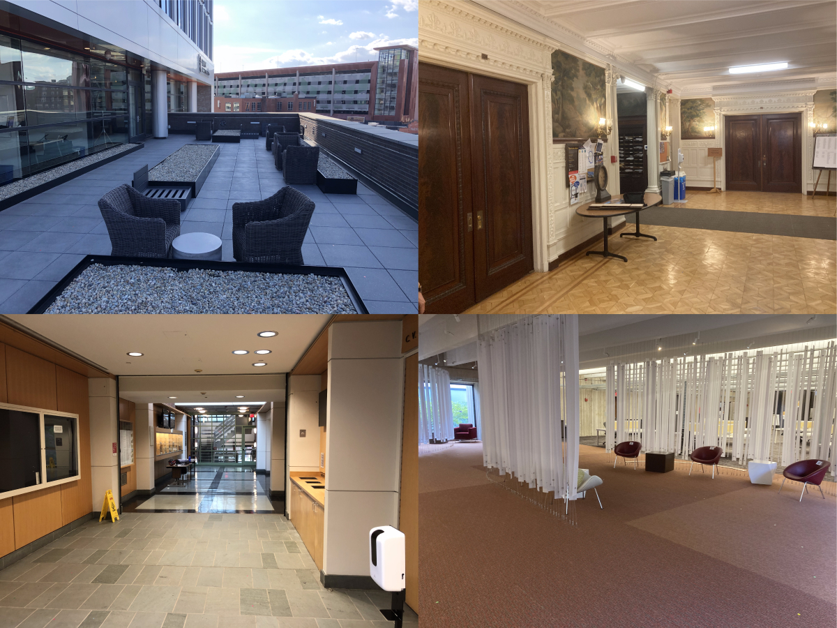
Figure 1: BPOD spans a diverse set of indoor and outdoor scenes ranging from texture-rich historic buildings to modern construction.

TABLE I: Comparison of representative datasets.

Dataset	Mounting	Environment	Camera Type	Image	Ground Truth
KITTI [30]	Car	Outdoors	Global Shutter	Stereo/Auto Exposure	GPS
EuRoc [31]	MAV	Indoors	Global Shutter	Stereo/Auto Exposure	Motion Capture
TUM [34]	Hand-held	Indoors	Global Shutter	Monocular/Auto Exposure	Motion Capture
ICL-NIUM [37]	Synthetic	Synthetic-Indoors	Synthetic	Monocular/Synthetic	Synthetic
MineNav [38]	Synthetic	Synthetic-Outdoors	Synthetic	Monocular/Synthetic	Synthetic
UMA-VI [32]	Hand-held	Indoor/Outdoors	Global Shutter	Stereo / Auto Exposure	SfM
PennCOSY [33]	Hand-held	Indoor/Outdoors	Mix	Stereo/Auto Exposure	Fiducial/SfM
BPOD (Ours)	Head-mount	Indoor/Outdoors	Mix	Stereo/Mix Exposure	Marker

Pedestrian tracking from head-mounted cameras is an application for which VO datasets are not available to the best of our knowledge. Existing datasets are commonly vehicle-mounted [13, 39, 40], Segway-mounted  [35], MAV-mounted [41, 36], or hand-held [42, 43, 44, 29]. The rare exception is one sequence (Campus-run) obtained from a head-mounted Velodyne LIDAR, but not from visual cameras. The authors included this sequence to highlight the added importance of the IMU in head-mounted situations which depict erratic movements [45]. As such, the proposed dataset, the Brown Pedestrian Odometry Dataset (BPOD), fills a gap in a significant application area.

A head-mounted camera presents challenges not always present in the other datasets: inherent in a head-mounted camera are erratic and rapid head movements. Also, pedestrians often make quick rotations, which leads to blur in images, as shown in Figure 2.

The creation of a VO-focused dataset like BPOD requires several components: (i) A sensory platform for data acquisition: we selected two synchronized stereo cameras, one with a rolling shutter and one with a global shutter. Embedded within the latter is an IMU. In addition, one camera can acquire depth images, although the current version of BPOD omits these in favor of higher resolution images and higher frame rates. (ii) Video sequences: ours are obtained from indoor and outdoor scenes by a pedestrian wearing the helmet following a path annotated on the ground by small markers. An additional camera records the pedestrian’s movement. (iii) Data processing to correlate pedestrian position to a map of markers to generate the ground-truth data. (iv) Experiments to evaluate the performance of VO algorithms: we tested three classes of odometry approaches on BPOD. The BPOD dataset is curated by the Brown University Library and is freely available for public use (the link will be included in the camera-ready version). Following a review of related datasets, this paper is organized according to these four components.

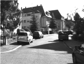
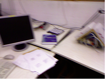
(a) (b) (c)

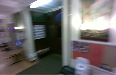
Figure 2: Typical turning sequences from vehicle-mounted (a), hand-held (b), and head-mounted (c) cameras demonstrate the potential for comparatively severe blur in head-mounted sequences.

II Related Odometry Datasets

Datasets focused on a variety of settings have been proposed to evaluate the performance of visual odometry systems. Perhaps the most well known is KITTI [30], which focuses on outdoor car-mounted stereo imaging, with ground-truth trajectories obtained via GPS. While this dataset showcases a diverse set of driving scenes, it is inherently limited by its outdoor, vehicle-focused setting. The EuRoC MAV datset [31] provides stereo images from a drone in an indoor environment. Its ground truth is captured by an external motion capture system and laser tracker. While this provides high-quality ground-truth trajectories, the necessary extra equipment requires a controlled environment, which prevents the creation of a large-scale dataset for indoor environments. The TUM RGB-D dataset [46] was one of the first datasets focused on hand-held cameras. It features a large set of hand-held video sequences, but the ground-truth timestamps are not well aligned with the camera. The ground truth of this dataset is also captured by an external motion capture system, so this dataset only covers limited range of scenes. Additionally, the motion of the hand-held camera is slow and smooth, which is appropriate for hand-held scanning applications, but not for pedestrian ego-motion estimation. To overcome the limitations of external motion capture systems, ground truths based on fiducial markers have been used in a number of datasets [33]. However, these prominent markers generate extra feature correspondences within the scene (note that the markers used for our ground truths are non-invasive). Following the development of structure from motion (SfM) techniques, several datasets have used SfM to generate ground-truth camera trajectories. For example, [32] and [47] use COLMAP and Pix4D respectively to generate their ground truths. However, unlike these carefully constructed hand-held and MAV datasets, our dataset contains rapid blur and feature-less segments that make SfM-based ground truth generation infeasible. Other datasets omit ground-truth trajectories entirely, instead relying on loop closure. For example, the TUM MonoVO [34] dataset, which features a large set of hand-held, photometrically calibrated, monocular footage, proposes an evaluation metric based on loop closure to evaluate VO without ground-truth trajectories.

TABLE II: The streams we recorded for each sensor.

Camera	Sensors	Resolution	Frame Rate (Hz)	Sensor Aspect Ratio	Focal Length	FOV	baseline	Shutter Type
D455	Color	1280 ×800	30	16:10	1.88mm	77∘	95mm	Global
	Stereo Monochrome	1280 ×800	30	8:5	1.93mm	100.6∘
D415	Color	1920 ×1080	30	16:9	1.88mm	77∘	55mm	Rolling
	Stereo Monochrome	1280 ×720	30	16:9	1.88mm	77∘

In the face of these difficulties in generating ground truths for real cameras, synthetic datasets have also been devised for VO development. The ICL-NUIM dataset [37] consists of 8 sequences of photorealistic synthetic indoor scenes in a monocular setting. The MineNav dataset [38] presents an outdoor odometry dataset based on the sandbox game Minecraft. However, it is hard for these synthetic datasets to simulate features of real scenes, such as motion blur and pedestrian head bobbing. A summary of representative datasets is listed in Table I.

III BPOD Sensory Platform

The camera mount most appropriate for pedestrian visual odometry is a head mount: cameras with chest-mounted or hand-held configurations are often occluded by the subject’s arms or the presence of other pedestrians. The BPOD camera rig is a ski helmet outfitted with a standard GoPro mount. Figure 3 shows the 3D-printed frame we used to attach our cameras to the helmet.

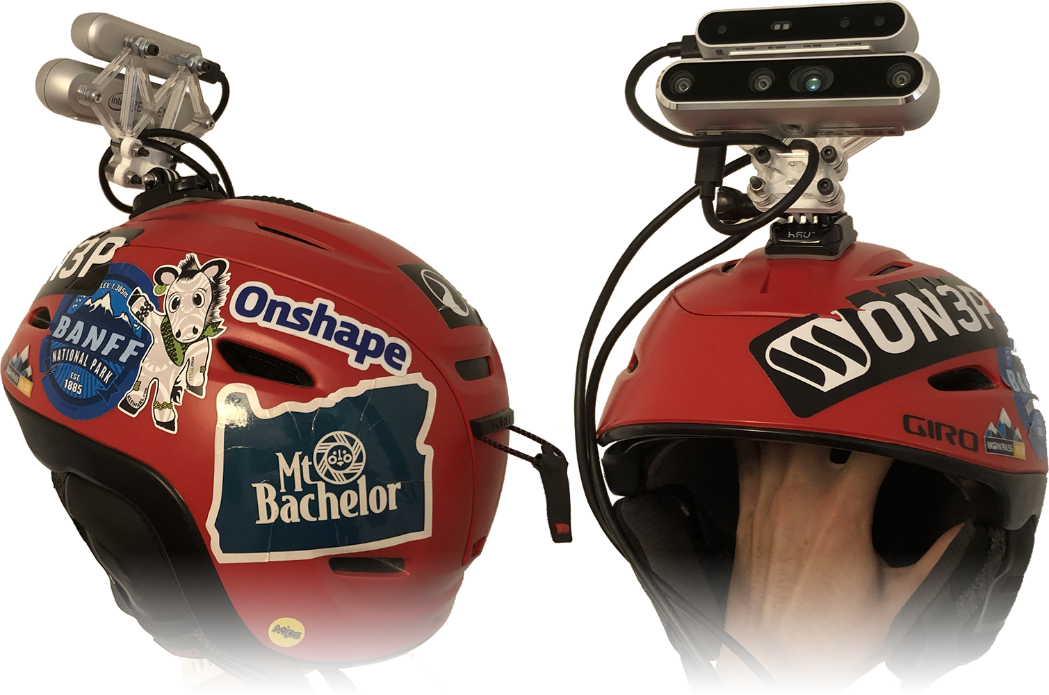
Figure 3: Two views of the camera assembly, shown together with frontal inter-camera measurements and CAD drawings.

Our camera selection was guided by several constraints: We required (i) synchronized stereo cameras to compare monocular and stereo configurations for pedestrian odometry; (ii) high image quality, resolution, and frame rate; (iii) exposure control to allow for precise photometric calibration; (iv) both rolling shutter and global shutter cameras for comparison; (v) a universal driver for compatibility with a variety of devices; (vi) an IMU; and (vii) consumer-level pricing.

Given these constraints, we chose a pair of Intel RealSense cameras [48] whose specifications are outlined in Table II. An additional advantage of this choice is the ability to capture depth maps, although we could not incorporate this feature into BPOD due to data transfer bandwidth constraints. A few competing choices were (i) oCam from WithRobot [49], which did not have exposure control and had inferior image quality; (ii) an ArduCam [50] which was limited to Nvidia Jetson or Raspberry Pi interfaces; and (iii) BumbleBee2 [51], a global shutter stereo camera which was discontinued by the manufacturer.

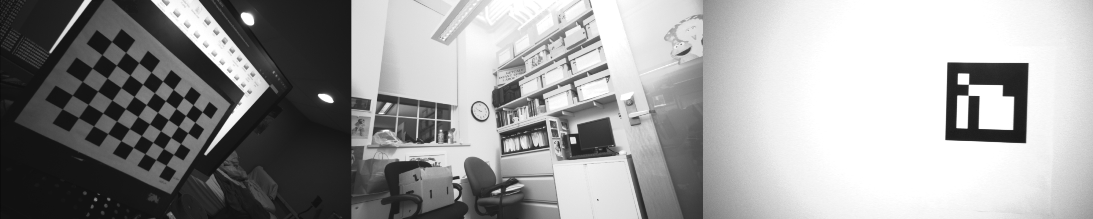
Figure 4: Left to right: A sample checker board image, an image in the sweep exposure set, and a sample vignette image used for calibration.

Intrinsic and Photometric Calibration: We calibrated the intrinsic parameters, distortion parameters, photometric parameters and vignette parameters for each camera independently. For each camera, we captured three calibration sequences: (i) A $10\times 7$ checker board for intrinsic calibration; (ii) a static scene with sweeping exposure for photometric calibration, and (iii) An image sequence with an ArUco tag [52] for vignette calibration, as shown in Figure 4. We estimated the intrinsic parameters and distortion parameters using the MATLAB calibration toolbox. We estimated the photometric and vignette parameters using the code provided by [34]. The extrinsic calibration for stereo cameras consists of the baseline listed in Table II. We extracted the relative pose between D455 and D415 camera from the design of the camera rig shown in Figure 3.

IMU Calibration: We used the RealSense Toolkit for IMU calibration to obtain intrinsic and extrinsic IMU calibrations, which are available in BPOD.

TABLE III: Basic Information of BPOD dataset

Location (Abbrev.)	Length of Sequences (sec.)
Applied Math Building (APMA)	86	86	84	84
85 Waterman St. (BERT)	102	96	106	100
Brown Design Workshop (BDW)	109	113	110	109
CIC Office Balcony (CIC)	122	141	140	145
Center of Info. Tech. (CIT 2nd Floor)	75	73	80	80
Center of Info. Tech. (CIT 4th Floor)	91	91	96	94
Lobby of Eng. Res. Center (ERC)	109	110	x	x
Lobby of Friedman Hall (Friedman)	95	97	99	98
Lobby of MacMillan Hall (MacMillian)	95	90	96	93
Science Lib. (SciLiTables)	68	67	69	74
Science Lib. (SciLiShutters)	84	82	100	84

IV Data Acquisition Protocol

BPOD sequences were recorded at 12 locations on Brown University’s campus, as outlined in Table III. We selected these locations to encompass a wide range of architectural styles, lighting conditions, and texture properties.

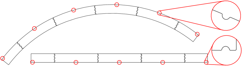
(a) CAD drawings of the templates used to place markers. Indentations for marker placement, which are spaced 30 inches apart, are highlighted and shown in detail views.

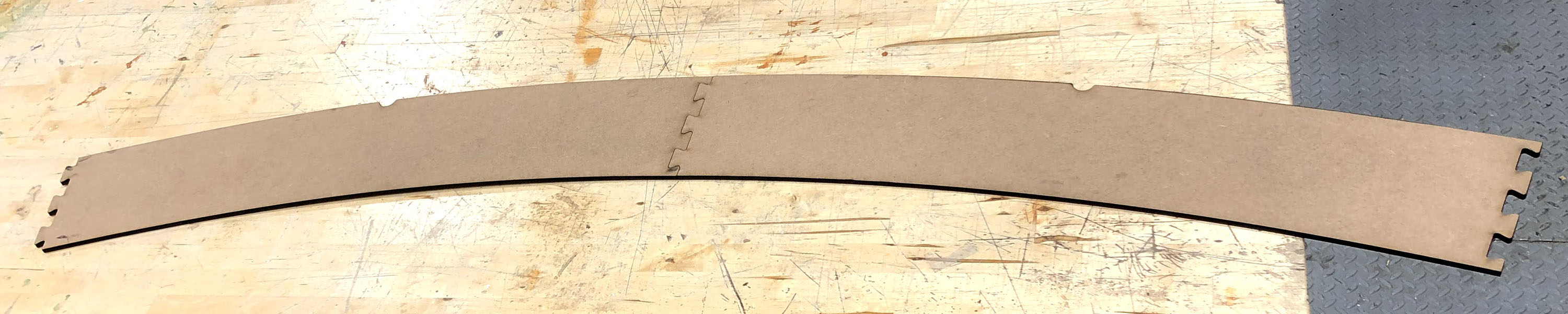
(b) Two laser-cut components for an arc template.

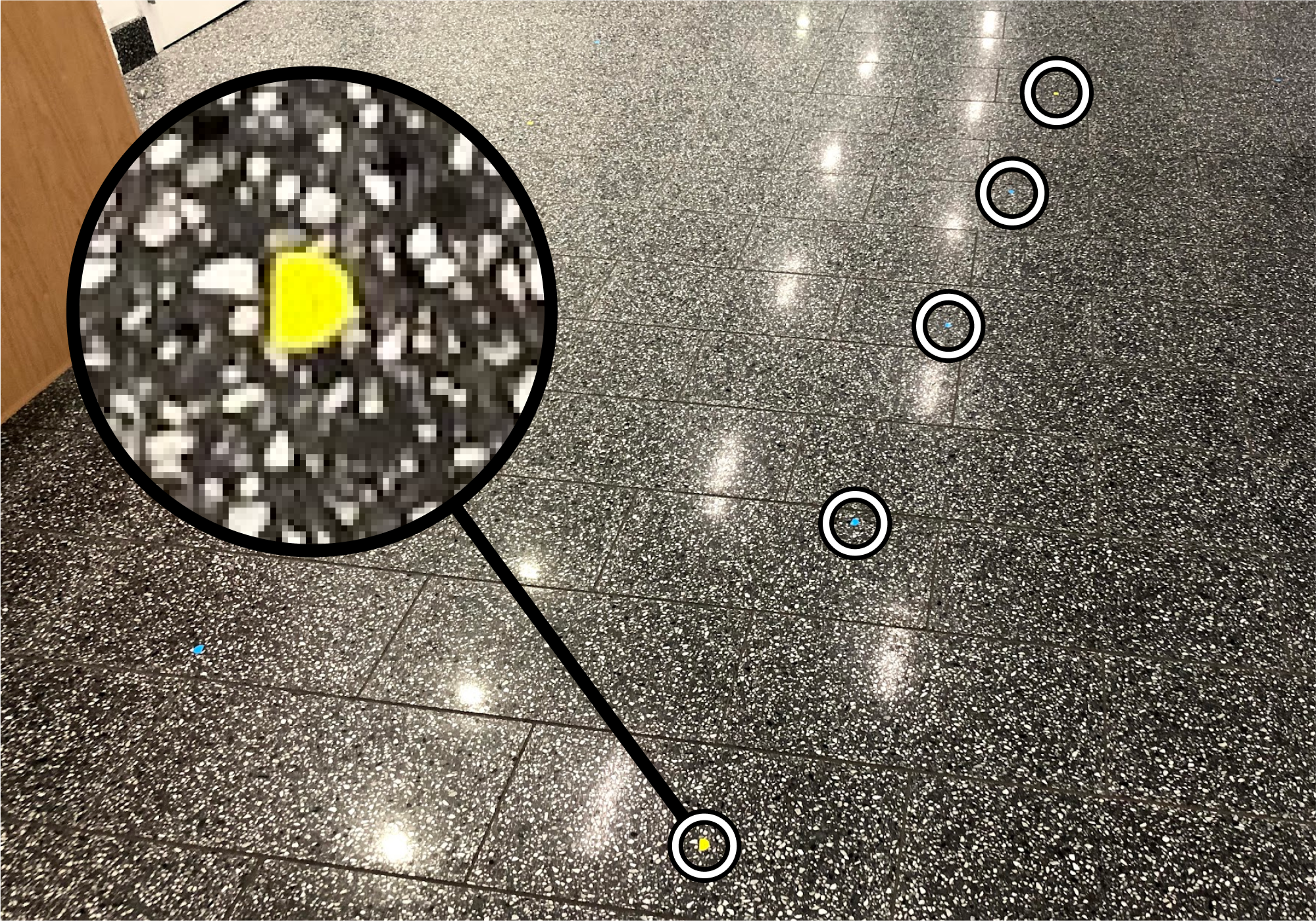
(c) Markers placed using the straight path segment. A key marker is highlighted.

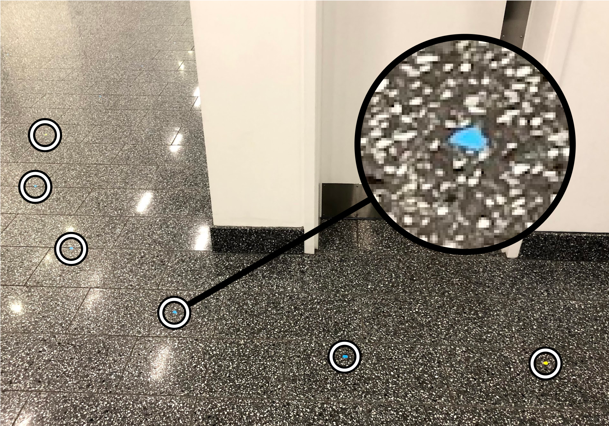
(d) Markers placed using the arc segment. An intermediate marker is highlighted.

Figure 5: Laser-cut templates and stick-on markers are used to generate ground-truth trajectories.

Defining Trajectories: We used sequences of sticker markers to define intended trajectories for our video sequences. We placed these markers at 30-inch intervals using two laser-cut templates as shown in Figure 5. One was a 120-inch straight template with slots for four markers, and a 90-degree circular arc template with slots for five markers. Our trajectories are closed loops, which allows the subject to traverse them multiple times in succession.

Mapping Trajectories: We used pairwise distance measurements between markers in conjunction with triangulation-based initialization and descent-based optimization to construct two-dimensional trajectory maps. We partitioned the markers into key markers and intermediate markers. Key markers used a distinct sticker color and were placed at the ends of templates, while intermediate markers filled the templates’ middle slots. From each key marker, we recorded distance measurements to all other non-occluded key markers using a hand-held Bosch Blaze Pro GLM165-40 laser distance measurer. Typically, about half of the other key markers were visible.

To convert sets of pairwise distance measurements to usable trajectories, we first generated coarse maps using classical triangulation. Recall that given the points $p_{1}$ at $(0,0)$ and $p_{2}$ at $(u,0)$, the position $(x,y)$ of a third point $p_{\text{unknown}}$ with distances $r_{1}$ to $p_{1}$ and $r_{2}$ to $p_{2}$ is given by the following equations:

An additional distance measurement between $p_{\text{unknown}}$ and a known position resolves $y$’s ambiguous sign. To apply this principle, we construct a graph $G$ where each key marker is a node, and each pairwise measurement between key markers forms an edge. Next, we form a subgraph $G_{\text{mapped}}$ from an arbitrary clique of size 3. We assign the first two markers positions of $(0,0)$ and $(u,0)$ respectively, where $u$ is the measured distance between the markers. Next, we use Equation 1 to determine the third marker’s position, assuming a positive value of $y$. We then iteratively add each remaining node in $G$ to $G_{\text{mapped}}$ when at least three of its neighbors are in $G_{\text{mapped}}$, triangulating nodes’ positions as they are added. If all markers can be triangulated, the initialization is complete; otherwise, we retry using a different initial clique. Note that because we assume a positive value of $y$ when triangulating the initial clique, we must manually reflect some of the resulting initializations about an arbitrary axis.

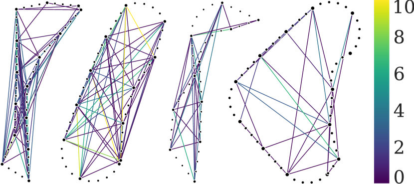
Figure 6: Maps showing measurements with their post-optimization errors for four locations. The legend’s unit is millimeters.

Once initialization is complete, we refine the map using gradient descent. We optimize the markers’ positions using an L1 loss $L=\sum_{i}{\lvert d_{i}-\hat{d}_{i}\rvert}$ between the measured distance $d_{i}$ and implied pairwise distances $\hat{d}_{i}$ between markers. This optimization generally leads to errors under 1cm (see Figure 6).

Discussion: Compared to more complex and costly ground truth generation schemes, e.g., laser trackers [53], our scheme trades temporal resolution and the availability of 6-DOF information for simplicity. However, we argue that a ground truth’s most important characteristic is that it provides accurate positional information over long distances, as this is essential for evaluating drift in odometry.

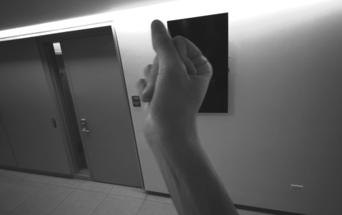
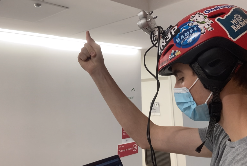
Figure 7: Finger snap synchronization of first-person (left) and third-person (right) video streams.

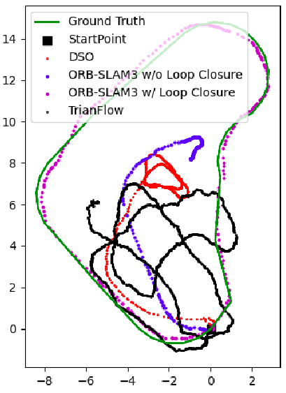
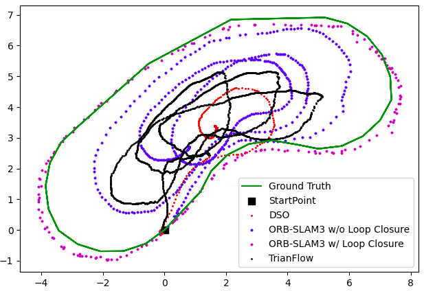
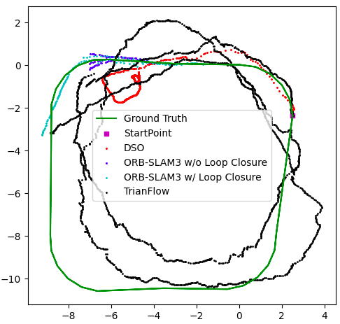
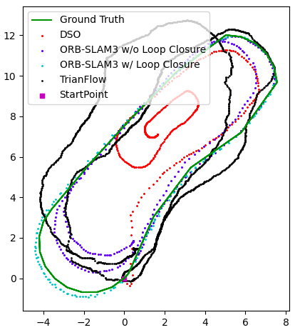
Figure 8: The estimated camera trajectories for four sample sequences.

Capturing video sequences: We used a Macbook Pro to record data from the camera rig. We additionally recorded third-person video of the subject’s feet with a smartphone to help reconstruct ground-truth trajectories. We synchronized the RealSense cameras and smartphone by starting each sequence with a finger snap, which is fast enough to ensure synchronization to within one frame, Figure 7.

$$x=\frac{r_{1}^{2}-r_{2}^{2}+u^{2}}{2u}\qquad y=\pm\sqrt{\lvert r_{1}^{2}-x^{2}\rvert}$$ (1)

We captured four videos for each trajectory along two axes of variation: forward vs. backward trajectory traversal and fixed vs. auto exposure. Each trajectory follows a loop that is traversed 2 to 4 times.

The idea of varying exposure is to probe the performance of various methods on scenes with a very high dynamic range of illumination. For example, the sequence “4th floor of CIT” transitions between a brightly lit atrium with skylights and a dimly lit set of hallways. We noted that the default setting of the auto-exposure mode is set relatively low, perhaps because it is intended to work with a laser projector. For the manually set exposure, we chose settings to balances overexposed (blown-out) regions and underexposed (completely black) regions.

Extracting the data: Each sequence produces two distinct Robot Operating System (ROS) bag files, one for D415 and one for D455, which contain all data. We used a Docker container running an Ubuntu image with ROS to extract PNG images, camera calibration parameters, and IMU data along with the corresponding timestamps.

Image Position Annotation: Our third-person smartphone videos allow us to identify the subject’s location with respect to the marker-defined map at each point in time. We annotated the times at which the subject crosses individual markers, then interpolated the corresponding times and positions to produce fine-grained ground truth data. Our ground-truth data defines time relative to the first frame after the snap. This allows the two cameras’ video streams to easily be synchronized with the smartphone’s video.

V Experiments

In this section, we describe the performance of three categories of visual odometry algorithms on BPOD. We selected a representative algorithm for each category: ORB-SLAM3 [54] for feature-based approaches, DSO [55] for direct approaches, and TrianFlow [28] (trained on TUM dataset) for deep learning approaches. Both TrianFlow and DSO are restricted to monocular inputs, so we ran all tests using ORB-SLAM3’s monocular mode. We use the authors’ implementations of their odometry algorithms for all experiments.

The evaluation of monocular odometry must address the inherent scale ambiguity in the resulting reconstructions: metric ambiguity in reconstruction and pose implies that scale as well as translation and rotation need to be matched optimally to compare two trajectories, i.e. two trajectories must by aligned under a similarity transformation. Observe that the ground truth of BPOD is in 2D while the computed odometry paths are in 3D. The latter are in fact fairly planar however, with small pseudo-sinusoidal depth variations that correspond to the bobbing head movements inherent to a pedestrian gait. Figure 8 compares the ground-truth trajectory to the reconstructed paths for each of the three approaches under the optimal similarity alignment constrained to matched start points (i.e. minimum distance under all relative relative rotations and scaling). It is clear that the reconstructed trajectories are not suitable for use in applications. In fact, these results are selected from among the very few sequences for which all methods completed the reconstruction of the trajectory!

A quantitative characterization of these results is shown in Table IV. A global evaluation metric $d_{e}$ measures the distance between the ground-truth and the estimated trajectories’ end points. Observe that only three of twelve locations are completed by ORB-SLAM, in contrast to DSO which completes over 85% of the locations and to TrianFlow which completes all; the endpoint error, $d_{e}$, however, is quite high for DSO and TrianFlow.

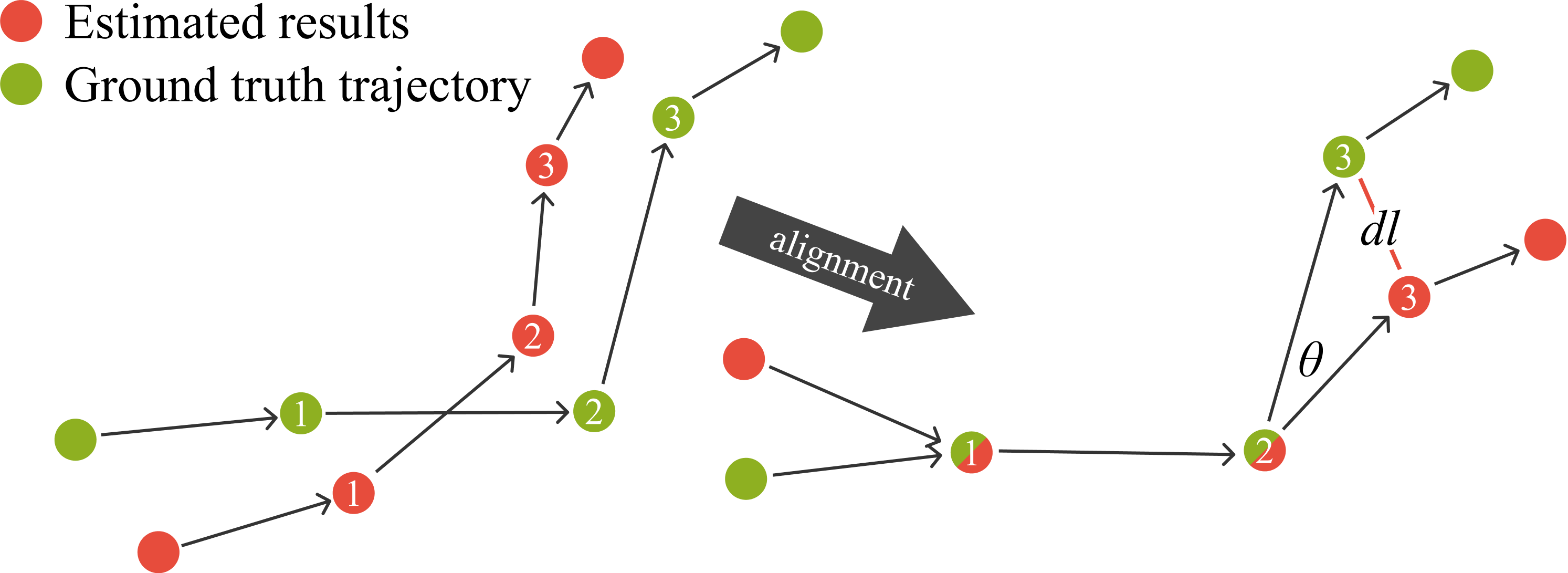
Figure 9: An illustration of our local error metrics.

TABLE IV: Benchmarks for Each Location (X: Lost Track; -: Estimated Trajectory is short)

Locations	ORB-SLAM w/o LC			ORB-SLAM w/ LC			DSO			TrianFlow
	$d_{e}$(m)	$\theta$(${}^{\circ}/s$)	$d_{l}$($m/s$)	$d_{e}$(m)	$\theta$(${}^{\circ}/s$)	$d_{l}$($m/s$)	$d_{e}$(m)	$\theta$(${}^{\circ}/s$)	$d_{l}$($m/s$)	$d_{e}$(m)	$\theta$(${}^{\circ}/s$)	$d_{l}$($m/s$)
APMA	X	1.44	0.09	X	1.15	0.09	3.73	4.13	0.27	4.20	8.80	0.43
BDW	X	-	-	X	-	-	7.62	3.23	0.22	6.48	6.27	0.42
BERT	X	0.83	0.12	X	0.52	0.12	4.25	14.2	0.69	7.29	7.75	0.53
CIC Balcony	X	6.3	0.63	X	7.00	1.99	4.33	8.64	0.11	5.21	8.22	0.67
CIT 2nd Floor	X	-	-	X	-	-	7.02	3.88	0.68	8.86	5.87	0.40
CIT 4th Floor	6.50	4.15	0.18	0.05	1.07	0.22	7.79	1.78	0.21	7.82	3.75	0.30
ERC	X	6.02	0.18	X	5.96	0.18	6.95	3.00	0.48	8.73	5.62	0.41
Friedman Hall	X	4.55	0.23	X	5.94	0.23	X	4.53	0.45	9.92	10.77	0.54
MacMillan	X	-	-	X	-	-	X	5.57	0.57	9.87	8.18	0.57
SciLiShutters	3.74	0.72	0.11	0.15	0.54	0.06	5.90	3.57	0.50	4.22	5.10	0.56
SciLiTables	1.39	0.40	0.06	0.09	0.41	0.06	5.34	0.80	0.14	5.45	2.73	0.41
MEAN	3.88	3.05	0.2	0.10	2.82	0.37	5.88	4.85	0.39	7.09	6.64	0.48

A closer look at the reconstructed path reveals that scale drift is a significant issue, especially for DSO. This implies that a single scaling of the reconstruction path will lead to a large $d_{e}$ even though the shape is correctly estimated. We propose to use a local metric to decouple the error caused by scale drift from the error in reconstructing the shape of the path. Figure 9 illustrates the idea: consider the samples along each path, say one second apart. Aligning the first two samples adjusts the local scale of the reconstructed path to be that of the ground truth. Then, difference between the third point, angular difference $\theta$ and magnitude difference $d_{l}$, reveral the local reconstruction error. The conclusion is (i) ORB-SLAM is the most accurate in reconstruct a trajectory, but it frequently fails to do so; this is due to fast rotations that cause motion blur and the subsequent loss of feature tracking. (ii) DSO frequently completes the trajectory but suffers from scale drift despite accurate calibration and use of global shutter cameras; (iii) TrianFlow completes all trajectories but is the least accurate.

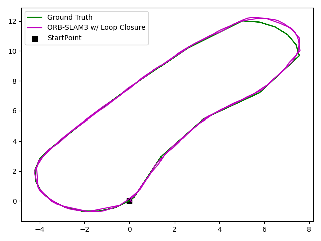
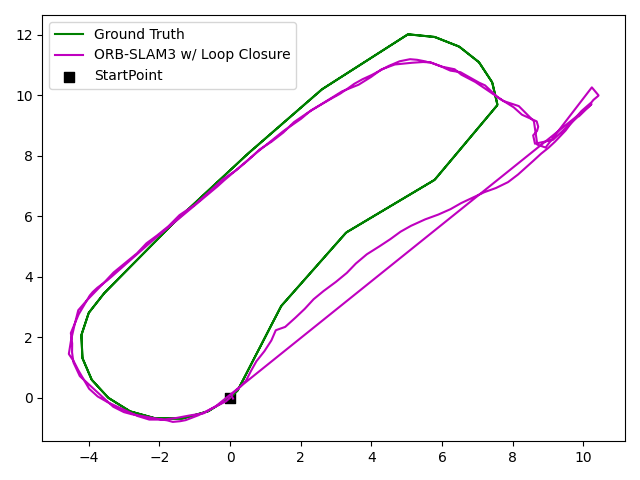
Figure 10: A comparison of ORB-SLAM3’s performance on global shutter (left) and rolling shutter (right) sequences.

Our experiments all used global shutter images, as the odometry results are generally better with these. Figure 10 compares ORB-SLAM3’s estimated trajectories for global and rolling shutter images. The availability of simultaneously obtained images from these two types of cameras allows a quantitative evaluation of the relative value of one camera vs. the other. This significant difference highlights the need for explicit models for rolling shutter cameras [56] and the usefulness of BPOD to evaluate the effectiveness of such explicit models.

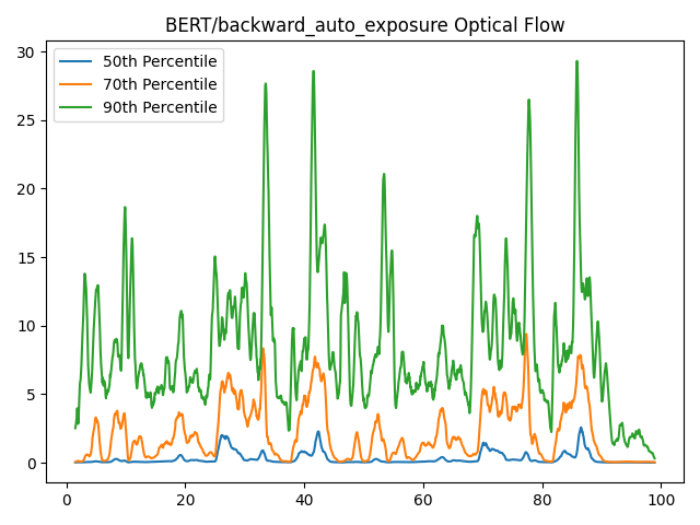
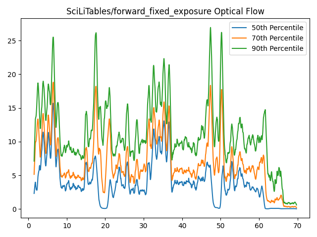
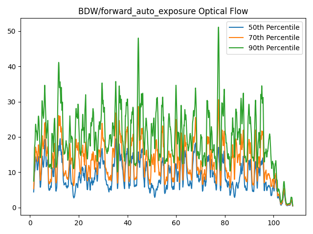
Figure 11: Plots of optical flow magnitude across our sequences show that BPOD is characterized by sudden, rapid movements that produce spikes in optical flow.

Finally, the use of optical flow magnitude was proposed by [53] to visualize the level of difficulty across sequences in the same dataset. Figure 11 shows this measure over several sequences in BPOD, highlighting spikes of very large median (300 pixels/s) and 90th percentile (800 pixels/s) magnitudes.

VI Conclusion

We developed a novel head-mounted pedestrian dataset based on 12 locations that cover a diverse set of scenes and illumination conditions. The dataset contains synchronized stereo data from both rolling shutter and global shutter cameras, enabling a comparison of the two for future algorithm development, and is supplemented with IMU data. Tests on three representative feature-based, direct, and deep learning methods reveal that the dataset contains challenges not previously addressed by existing datasets. We hope that the BPOD dataset will facilitate the development of more reliable and accurate odometry methods to address the unique challenges of head-mounted pedestrian odometry.

References

- [1] D. Nistér, O. Naroditsky, and J. Bergen, “Visual odometry,” in Proceedings of the 2004 IEEE Computer Society Conference on Computer Vision and Pattern Recognition, 2004. CVPR 2004., vol. 1. IEEE, 2004, pp. I–I.
- [2] D. Scaramuzza and F. Fraundorfer, “Visual odometry [tutorial],” IEEE robotics & automation magazine, vol. 18, no. 4, pp. 80–92, 2011.
- [3] F. Fraundorfer and D. Scaramuzza, “Visual odometry: Part ii: Matching, robustness, optimization, and applications,” IEEE Robotics & Automation Magazine, vol. 19, no. 2, pp. 78–90, 2012.
- [4] R. Mur-Artal, J. M. M. Montiel, and J. D. Tardos, “Orb-slam: a versatile and accurate monocular slam system,” IEEE transactions on robotics, vol. 31, no. 5, pp. 1147–1163, 2015.
- [5] R. Mur-Artal and J. D. Tardós, “Orb-slam2: An open-source slam system for monocular, stereo, and rgb-d cameras,” IEEE transactions on robotics, vol. 33, no. 5, pp. 1255–1262, 2017.
- [6] R. A. Newcombe, S. J. Lovegrove, and A. J. Davison, “Dtam: Dense tracking and mapping in real-time,” in 2011 international conference on computer vision. IEEE, 2011, pp. 2320–2327.
- [7] J. Engel, V. Koltun, and D. Cremers, “Direct sparse odometry,” IEEE transactions on pattern analysis and machine intelligence, vol. 40, no. 3, pp. 611–625, 2017.
- [8] K. Tsotsos, A. Chiuso, and S. Soatto, “Robust inference for visual-inertial sensor fusion,” in 2015 IEEE International Conference on Robotics and Automation (ICRA). IEEE, 2015, pp. 5203–5210.
- [9] D. Scaramuzza and Z. Zhang, “Visual-inertial odometry of aerial robots,” arXiv preprint arXiv:1906.03289, 2019.
- [10] M. Blösch, S. Weiss, D. Scaramuzza, and R. Siegwart, “Vision based mav navigation in unknown and unstructured environments,” in 2010 IEEE International Conference on Robotics and Automation. IEEE, 2010, pp. 21–28.
- [11] I. Cvišić, J. Ćesić, I. Marković, and I. Petrović, “Soft-slam: Computationally efficient stereo visual simultaneous localization and mapping for autonomous unmanned aerial vehicles,” Journal of field robotics, vol. 35, no. 4, pp. 578–595, 2018.
- [12] H. Lategahn, A. Geiger, and B. Kitt, “Visual slam for autonomous ground vehicles,” in 2011 IEEE International Conference on Robotics and Automation. IEEE, 2011, pp. 1732–1737.
- [13] A. Geiger, P. Lenz, and R. Urtasun, “Are we ready for autonomous driving? the kitti vision benchmark suite,” in 2012 IEEE conference on computer vision and pattern recognition. IEEE, 2012, pp. 3354–3361.
- [14] D. Chekhlov, A. P. Gee, A. Calway, and W. Mayol-Cuevas, “Ninja on a plane: Automatic discovery of physical planes for augmented reality using visual slam,” in 2007 6th IEEE and ACM International Symposium on Mixed and Augmented Reality. IEEE, 2007, pp. 153–156.
- [15] S. Karam, G. Vosselman, M. Peter, S. Hosseinyalamdary, and V. Lehtola, “Design, calibration, and evaluation of a backpack indoor mobile mapping system,” Remote sensing, vol. 11, no. 8, p. 905, 2019.
- [16] X. Shi, D. Li, P. Zhao, Q. Tian, Y. Tian, Q. Long, C. Zhu, J. Song, F. Qiao, L. Song, et al., “Are we ready for service robots? the openloris-scene datasets for lifelong slam,” in 2020 IEEE International Conference on Robotics and Automation (ICRA). IEEE, 2020, pp. 3139–3145.
- [17] T. Bailey and H. Durrant-Whyte, “Simultaneous localization and mapping (slam): Part ii,” IEEE Robotics & Automation Magazine, vol. 13, no. 3, pp. 108–117, 2006.
- [18] H. Durrant-Whyte and T. Bailey, “Simultaneous localization and mapping: part i,” IEEE robotics & automation magazine, vol. 13, no. 2, pp. 99–110, 2006.
- [19] C. Cadena, L. Carlone, H. Carrillo, Y. Latif, D. Scaramuzza, J. Neira, I. Reid, and J. J. Leonard, “Past, present, and future of simultaneous localization and mapping: Toward the robust-perception age,” IEEE Transactions on robotics, vol. 32, no. 6, pp. 1309–1332, 2016.
- [20] G. Pandey, J. R. McBride, and R. M. Eustice, “Ford campus vision and lidar data set,” The International Journal of Robotics Research, vol. 30, no. 13, pp. 1543–1552, 2011.
- [21] W. Maddern, G. Pascoe, C. Linegar, and P. Newman, “1 year, 1000 km: The oxford robotcar dataset,” The International Journal of Robotics Research, vol. 36, no. 1, pp. 3–15, 2017.
- [22] F. Yu, H. Chen, X. Wang, W. Xian, Y. Chen, F. Liu, V. Madhavan, and T. Darrell, “Bdd100k: A diverse driving dataset for heterogeneous multitask learning,” in Proceedings of the IEEE/CVF conference on computer vision and pattern recognition, 2020, pp. 2636–2645.
- [23] A. Antonini, W. Guerra, V. Murali, T. Sayre-McCord, and S. Karaman, “The blackbird dataset: A large-scale dataset for uav perception in aggressive flight,” in International Symposium on Experimental Robotics. Springer, 2018, pp. 130–139.
- [24] R. Mur-Artal, J. M. M. Montiel, and J. D. Tardos, “Orb-slam: a versatile and accurate monocular slam system,” IEEE transactions on robotics, vol. 31, no. 5, pp. 1147–1163, 2015.
- [25] S. Wang, R. Clark, H. Wen, and N. Trigoni, “Deepvo: Towards end-to-end visual odometry with deep recurrent convolutional neural networks,” in 2017 IEEE International Conference on Robotics and Automation (ICRA). IEEE, 2017, pp. 2043–2050.
- [26] R. Li, S. Wang, Z. Long, and D. Gu, “Undeepvo: Monocular visual odometry through unsupervised deep learning,” in 2018 IEEE international conference on robotics and automation (ICRA). IEEE, 2018, pp. 7286–7291.
- [27] N. Yang, L. v. Stumberg, R. Wang, and D. Cremers, “D3vo: Deep depth, deep pose and deep uncertainty for monocular visual odometry,” in Proceedings of the IEEE/CVF Conference on Computer Vision and Pattern Recognition, 2020, pp. 1281–1292.
- [28] W. Zhao, S. Liu, Y. Shu, and Y.-J. Liu, “Towards better generalization: Joint depth-pose learning without posenet,” in Proceedings of the IEEE/CVF Conference on Computer Vision and Pattern Recognition, 2020, pp. 9151–9161.
- [29] M. Kasper, S. McGuire, and C. Heckman, “A benchmark for visual-inertial odometry systems employing onboard illumination,” in 2019 IEEE/RSJ International Conference on Intelligent Robots and Systems (IROS). IEEE, 2019, pp. 5256–5263.
- [30] A. Geiger, P. Lenz, C. Stiller, and R. Urtasun, “Vision meets robotics: The kitti dataset,” The International Journal of Robotics Research, vol. 32, no. 11, pp. 1231–1237, 2013.
- [31] M. Burri, J. Nikolic, P. Gohl, T. Schneider, J. Rehder, S. Omari, M. W. Achtelik, and R. Siegwart, “The euroc micro aerial vehicle datasets,” The International Journal of Robotics Research, vol. 35, no. 10, pp. 1157–1163, 2016.
- [32] D. Zuñiga-Noël, A. Jaenal, R. Gomez-Ojeda, and J. Gonzalez-Jimenez, “The uma-vi dataset: Visual–inertial odometry in low-textured and dynamic illumination environments,” The International Journal of Robotics Research, vol. 39, no. 9, pp. 1052–1060, 2020.
- [33] B. Pfrommer, N. Sanket, K. Daniilidis, and J. Cleveland, “Penncosyvio: A challenging visual inertial odometry benchmark,” in 2017 IEEE International Conference on Robotics and Automation (ICRA). IEEE, 2017, pp. 3847–3854.
- [34] J. Engel, V. Usenko, and D. Cremers, “A photometrically calibrated benchmark for monocular visual odometry,” arXiv preprint arXiv:1607.02555, 2016.
- [35] N. Carlevaris-Bianco, A. K. Ushani, and R. M. Eustice, “University of michigan north campus long-term vision and lidar dataset,” The International Journal of Robotics Research, vol. 35, no. 9, pp. 1023–1035, 2016.
- [36] A. L. Majdik, C. Till, and D. Scaramuzza, “The zurich urban micro aerial vehicle dataset,” The International Journal of Robotics Research, vol. 36, no. 3, pp. 269–273, 2017.
- [37] A. Handa, T. Whelan, J. McDonald, and A. J. Davison, “A benchmark for rgb-d visual odometry, 3d reconstruction and slam,” in 2014 IEEE international conference on Robotics and automation (ICRA). IEEE, 2014, pp. 1524–1531.
- [38] D. Wang, “Minenav: An expandable synthetic dataset based on minecraft for aircraft visual navigation,” arXiv preprint arXiv:2008.08454, 2020.
- [39] J.-L. Blanco-Claraco, F.-A. Moreno-Duenas, and J. González-Jiménez, “The málaga urban dataset: High-rate stereo and lidar in a realistic urban scenario,” The International Journal of Robotics Research, vol. 33, no. 2, pp. 207–214, 2014.
- [40] J. Jeong, Y. Cho, Y.-S. Shin, H. Roh, and A. Kim, “Complex urban dataset with multi-level sensors from highly diverse urban environments,” The International Journal of Robotics Research, vol. 38, no. 6, pp. 642–657, 2019.
- [41] M. Burri, J. Nikolic, P. Gohl, T. Schneider, J. Rehder, S. Omari, M. W. Achtelik, and R. Siegwart, “The euroc micro aerial vehicle datasets,” The International Journal of Robotics Research, vol. 35, no. 10, pp. 1157–1163, 2016.
- [42] B. Pfrommer, N. Sanket, K. Daniilidis, and J. Cleveland, “Penncosyvio: A challenging visual inertial odometry benchmark,” in 2017 IEEE International Conference on Robotics and Automation (ICRA). IEEE, 2017, pp. 3847–3854.
- [43] D. Schubert, T. Goll, N. Demmel, V. Usenko, J. Stückler, and D. Cremers, “The tum vi benchmark for evaluating visual-inertial odometry,” in 2018 IEEE/RSJ International Conference on Intelligent Robots and Systems (IROS). IEEE, 2018, pp. 1680–1687.
- [44] S. Cortés, A. Solin, E. Rahtu, and J. Kannala, “Advio: An authentic dataset for visual-inertial odometry,” in Proceedings of the European Conference on Computer Vision (ECCV), 2018, pp. 419–434.
- [45] F. Neuhaus, T. Koß, R. Kohnen, and D. Paulus, “Mc2slam: Real-time inertial lidar odometry using two-scan motion compensation,” in German Conference on Pattern Recognition. Springer, 2018, pp. 60–72.
- [46] J. Sturm, N. Engelhard, F. Endres, W. Burgard, and D. Cremers, “A benchmark for the evaluation of rgb-d slam systems,” in Proc. of the International Conference on Intelligent Robot Systems (IROS), Oct. 2012.
- [47] A. L. Majdik, C. Till, and D. Scaramuzza, “The zurich urban micro aerial vehicle dataset,” The International Journal of Robotics Research, vol. 36, no. 3, pp. 269–273, 2017.
- [48] L. Keselman, J. Iselin Woodfill, A. Grunnet-Jepsen, and A. Bhowmik, “Intel realsense stereoscopic depth cameras,” in Proceedings of the IEEE Conference on Computer Vision and Pattern Recognition Workshops, 2017, pp. 1–10.
- [49] oCam Camera. [Online]. Available: http://withrobot.com/en/camera/ocams-1mgn-u/
- [50] ArduCam Camera. [Online]. Available: https://www.arducam.com/
- [51] BumbleBee Camera. [Online]. Available: https://www.flir.com/support/products/bumblebee2-firewire/#Overview
- [52] S. Garrido-Jurado, R. Muñoz-Salinas, F. J. Madrid-Cuevas, and M. J. Marín-Jiménez, “Automatic generation and detection of highly reliable fiducial markers under occlusion,” Pattern Recognition, vol. 47, no. 6, pp. 2280–2292, 2014.
- [53] J. Delmerico, T. Cieslewski, H. Rebecq, M. Faessler, and D. Scaramuzza, “Are we ready for autonomous drone racing? the uzh-fpv drone racing dataset,” in 2019 International Conference on Robotics and Automation (ICRA). IEEE, 2019, pp. 6713–6719.
- [54] C. Campos, R. Elvira, J. J. G. Rodríguez, J. M. Montiel, and J. D. Tardós, “Orb-slam3: An accurate open-source library for visual, visual–inertial, and multimap slam,” IEEE Transactions on Robotics, 2021.
- [55] J. Engel, V. Koltun, and D. Cremers, “Direct sparse odometry,” IEEE transactions on pattern analysis and machine intelligence, vol. 40, no. 3, pp. 611–625, 2017.
- [56] C. Albl, Z. Kukelova, V. Larsson, and T. Pajdla, “Rolling shutter camera absolute pose,” IEEE transactions on pattern analysis and machine intelligence, vol. 42, no. 6, pp. 1439–1452, 2019.