Optimal Variable Clustering for
High-Dimensional Matrix Valued Data
Abstract
Matrix valued data has become increasingly prevalent in many applications. Most of the existing clustering methods for this type of data are tailored to the mean model and do not account for the dependence structure of the features, which can be very informative, especially in high-dimensional settings or when mean information is not available. To extract the information from the dependence structure for clustering, we propose a new latent variable model for the features arranged in matrix form, with some unknown membership matrices representing the clusters for the rows and columns. Under this model, we further propose a class of hierarchical clustering algorithms using the difference of a weighted covariance matrix as the dissimilarity measure. Theoretically, we show that under mild conditions, our algorithm attains clustering consistency in the high-dimensional setting. While this consistency result holds for our algorithm with a broad class of weighted covariance matrices, the conditions for this result depend on the choice of the weight. To investigate how the weight affects the theoretical performance of our algorithm, we establish the minimax lower bound for clustering under our latent variable model in terms of some cluster separation metric. Given these results, we identify the optimal weight in the sense that using this weight guarantees our algorithm to be minimax rate-optimal. The practical implementation of our algorithm with the optimal weight is also discussed. Simulation studies show that our algorithm performs better than existing methods in terms of the adjusted Rand index (ARI). The method is applied to a genomic dataset and yields meaningful interpretations.
Keywords: Clustering, matrix data, high dimensional estimation, minimax optimality, latent variable model, hierarchical algorithm
1 Introduction
Cluster analysis is one of the most important unsupervised learning techniques and has been widely used to discover the underlying group structure in data, arising in many applications including economics, image analysis, psychology and the biomedical sciences (Everitt et al., 2011; Kogan, 2007). In these applications, matrix valued data is becoming increasingly prevalent. For example, in genetic studies, one may observe data matrices of dimension from subjects, where the th entry corresponds to the expression value of the th gene at the th tissue (Zahn et al., 2007). The biologist is often interested in identifying clusters of genes that share similar biological functions and also clusters of similar tissues. Similarly, in functional magnetic resonance imaging (fMRI) studies, to understand how the brain connectivity structure changes under different tasks/stimuli, researchers can measure the blood oxygen level (BOLD) within each region of interest (ROI) from the brain under a variety of conditions (Mitchell et al., 2008). The data points from each participant can be stacked as a matrix, in which the rows and columns correspond to different ROIs and tasks/stimuli, respectively. Given the data from participants, it is of interest to simultaneously cluster the ROIs and tasks/stimuli. Such clustering results can be used as a dimension reduction step to further investigate brain connectivity networks (Eisenach et al., 2020). However, in many cases such as when doing genetic studies, the data is already pre-processed and centered, and this loss of mean information prevents the use of existing mean-based clustering methods. Driven by these applications and limitations of existing methods, the goal of this paper is to develop a statistical clustering framework and a feasible algorithm for matrix valued data that utilizes covariance information with good theoretical guarantees. In particular, assuming that i.i.d. samples of a random matrix are observed, we aim to recover the cluster membership of the rows and columns of the feature matrix .
In the literature, clustering a data matrix is often known as biclustering (Hartigan, 1972; Madeira and Oliveira, 2004). Most of the existing biclustering methods can be classified into the following categories: (1) hierarchical approaches based on the dendrogram (Hastie et al., 2009); (2) extensions of K-means (Fraiman and Li, 2022); (3) the penalized likelihood approach (Tan and Witten, 2014); (4) convex clustering via fused lasso (Chi et al., 2017); and (5) clustering based on the singular value decomposition (Sill et al., 2011; Lee et al., 2010). In these existing works, the goal is to simultaneously cluster samples and features stacked as an data matrix, whereas in our problem we are interested in clustering a feature matrix. Since the features are often correlated, the feature matrix induces a sophisticated but informative dependence structure that is not accounted for in the existing biclustering literature. When also considering that there are instances where the data lacks mean information completely as in the case of centered gene-tissue data, it is apparent that there is a gap between existing biclustering methods and methods needed in various applications. More recently, multiway clustering, also known as tensor clustering, is attracting increasing attention (Mankad and Michailidis, 2014; Zhao et al., 2016; Chi et al., 2020; Sun and Li, 2019; Wang et al., 2019; Wang and Zeng, 2019). Since we observe i.i.d feature matrices, we can view our data as a 3-way tensor with dimension . The existing tensor clustering methods such as the tensor block model (Wang and Zeng, 2019; Chi et al., 2020) aim to cluster each mode of the tensor from the mean model. While these approaches enjoy great success in many applications and can be adapted to our setting, they may not perform well when the dependence structure of the features holds more information than the mean structure. There are also several recent works on tensor clustering that utilize some sort of dependence structure (Deng and Zhang (2022), Mai et al. (2022)), but these methods focus on clustering over the observations and not over the features (i.e., the rows and the columns of ) and thus is not directly applicable to our setting.
In this paper, our first contribution is to propose a new latent variable model for clustering matrix valued data. Assume the features are stacked as a random matrix , which follows
| (1.1) |
where without loss of generality, is a latent variable matrix with . and are the unknown binary membership matrices for the rows and columns, respectively, and represents the random noise matrix with entries that have mean 0 and variance . We assume that the entries in the noise matrix are mutually independent and are also independent of the entries in . Entries of the membership matrix take values in , such that if row belongs to row cluster and otherwise. In this paper, we focus on the non-overlapping and exhaustive clustering scenario. That is, for each row , there exists one and only one cluster with . The same requirement holds for the membership matrix . To see why and are interpreted as membership matrices, we note that, for any feature , if and for some and , then model (1.1) implies . That is, it implies that the feature is associated with the latent variable . For this reason, we say that belongs to row cluster and column cluster . Under model (1.1), we can formally define the row clusters as the partition
| (1.2) |
for any , where is the unknown number of row clusters. When the context is clear, will be used for notational simplicity. Without loss of generality, we focus on how to recover the unknown membership matrix for the rows (or equivalently ) up to label switching.
Model (1.1) can be viewed as the extension of the G-block model for clustering a random vector in Bunea et al. (2020) to matrix valued data. Indeed, if we vectorize the matrix , model (1.1) is equivalent to with , where denotes the vectorization of , formed by stacking the columns of into a single column vector, and denotes the Kronecker product. Thus, compared to Bunea et al. (2020) which allows to be any unstructured membership matrix, we impose the Kronecker product structure to the membership matrix . While our model for is more restrictive than the model in Bunea et al. (2020), it actually comes with two advantages for matrix clustering. First, as seen above, and are interpreted as the membership matrices for the rows and columns. Ignoring the Kronecker product structure and directly applying the model in Bunea et al. (2020) would no longer produce interpretable results for matrix clustering, as shown in Figure 3 in Section A in the Supplementary Material. Second, the Kronecker product of and provides a more parsimonious parametrization for the unknown membership matrix , leading to stronger theoretical guarantees on clustering.
It is also worth mentioning that our proposed latent variable model shares similarities with the stochastic block model (SBM) widely used in community detection in network analysis. First introduced in Holland et al. (1983), the stochastic block model assumes that nodes of a network are partitioned into subgroups called blocks and the distribution of the ties between nodes is dependent on the blocks to which the nodes belong. More specifically, they imposed the model where is the adjacency matrix, is the binary block membership matrix and is the matrix whose element represents the probability that a node from block is connected to a node in block . We defer the details on further development of the method to Airoldi et al. (2008); Zhang et al. (2020); Abbe (2017) and the references therein. It must be noted, however, that community detection with stochastic block type models is inherently different from our setting since the former is focused on clustering the nodes (i.e., the samples), whereas our matrix clustering setting is focused on clustering the features (the rows and the columns of ).
Our second contribution is to propose a class of hierarchical clustering methods based on the weighted covariance matrix for some pre-specified positive semi-definite matrix with the aim to recover the unknown membership matrix (and similarly for as well). We use the difference in entries of this weighted covariance matrix to define the dissimilarity measure in our hierarchical algorithm to recover the membership matrix . To establish the theoretical guarantees of our algorithm, we introduce the metric to quantify how well the clusters are separated. The precise definition is detailed in Section 3.1. Theoretically, we develop a general result on the clustering consistency of our hierarchical algorithm that holds for a broad class of weight matrices . To attain clustering consistency for the rows, we require the cluster separation metric to be no smaller than the order of , where is the unknown number of column clusters. The implication is that with the help of a larger , clustering the rows of becomes easier.
To investigate the optimality of our algorithm, we establish the minimax lower bound for clustering under our latent variable model. While the clustering consistency property holds for a broad class of weight matrices , our algorithm with a generic weight may not be minimax optimal. To derive an optimal clustering algorithm for the rows, the key is to account for the information in the column clusters. The intuition is that with a more accurate column cluster result, we can decorrelate the dependence structure of and reduce the noise induced by , which in turn improves the clustering accuracy for the rows. Following this argument, we define the optimal weight , and propose to estimate it by , where is an estimate of the column membership matrix and denotes the estimated number of clusters obtained from . Under mild conditions, we show that the proposed algorithm with the estimated optimal weight attains the minimax lower bound, and therefore is rate-optimal for clustering. To the best of our knowledge, our paper is the first to formally establish minimax optimality for clustering matrix valued data. From a technical perspective, to show the optimality of our algorithm, the main challenge is to quantify the stability of the algorithm with respect to an imperfect estimate as the weight matrix. In Section 4 we provide sufficient conditions to show the stability of the algorithm under some additional modeling assumptions. In practice, the hierarchical algorithm can be applied iteratively to cluster the rows and columns for increased accuracy. Finally, we conduct extensive numerical studies to support our theoretical results.
The rest of the paper is organized as follows. In Section 2, we propose the hierarchical algorithm and discuss the advantage of using the optimal weight, . In Section 3, we define a notion of cluster separation and use it to establish the clustering consistency of our algorithm and to derive the minimax lower bound. Since the algorithm using the optimal weight depends on the initial estimate , in Section 4, we verify the cluster separation condition and stability condition required in Theorem 3.1 for clustering consistency in matrix normal models. The practical implementation of the algorithm is discussed in Section 5. Three further extensions of our method - the dependent noise model, the nested clustering method to incorporate both mean and covariance information, and higher order tensor models - are discussed in Section 6. The simulation results and real data analysis are presented in Sections 7 and 8, respectively. The paper concludes with a discussion in Section 9.
Notation. For any , we write if and are in the same cluster (i.e., for some ). Otherwise, we write . For a matrix , we use the following norms: , , . denotes the largest singular value of . The largest and smallest eigenvalues are denoted by and . We use and to denote the th column and row of , respectively. For two positive sequences and , we write if for all for some constant . Similarly, we use () to denote () for all for some constant .
2 Methodology
2.1 Hierarchical Clustering via Weighted Covariance Differences
Recall that the random matrix follows model (1.1). In this section, we propose a class of clustering methods for the rows of based on the weighted covariance matrix , where is some positive semi-definite matrix to be chosen. We add a subscript to indicate is a matrix corresponding to the rows. The same type of method can be used to cluster the columns of .
In the following, we first outline how to identify the unknown membership matrix from the weighted covariance matrix on the population level. Under model (1.1), by the independence between and , we obtain that
| (2.1) |
To recover the membership matrix from , one needs to first separate the two matrices and . Noting that is a diagonal matrix as the elements in are mutually independent and the weight matrix is deterministic, we therefore focus on the non-diagonal entries of , that is for any . By the definition of the membership matrix , for any , and , we have
| (2.2) |
In view of (2.2), the within-cluster covariance difference with is always 0 for any . In other words, as long as is nonzero for some , it indicates that and are not in the same cluster. Thus, the covariance difference is indicative of the clustering structure. Following Bunea et al. (2020), we formally define the covariance difference (cod) as
| (2.3) |
From the above argument, we have if . Moreover, if holds for all , we are able to identify all the clusters. Let
| (2.4) |
denote the minimum cod value over all possible . On the population level, provided , the membership matrix (or equivalently in (1.2)) is identifiable from the weighted covariance matrix up to label switching.
Based on the above results on the population level, we will develop a hierarchical clustering algorithm to estimate the membership matrix (or equivalently in (1.2)). Given i.i.d. samples , we first estimate with
and then plug this into (2.3) to form a dissimilarity measure for any . The hierarchical algorithm starts with every variable representing a singleton cluster. At each step, the closest two clusters are merged into one single cluster based on the following dissimilarity measure between two sets and
| (2.5) |
We refer to Hastie et al. (2009) for alternative definitions of dissimilarity between two clusters and further discussions. Finally, we terminate this process and report the clusters when the dissimilarity measure exceeds a threshold value . This hierarchical algorithm, summarized in Algorithm 1, improves the existing cod algorithm proposed by Bunea et al. (2020). First, our algorithm satisfies the so-called monotonicity property, which states that merged clusters always have smaller values of than unmerged ones (Hastie et al., 2009). However, the algorithm in Bunea et al. (2020) may merge indices and into one cluster even if there exists another index with smaller than . We include in Section B in the Supplementary Material a toy example that illustrates this point. Empirically, we find that our hierarchical algorithm produces more stable clustering results than the algorithm in Bunea et al. (2020). Second, the hierarchical algorithm is more flexible in incorporating side information, such as the number of row clusters . While our Algorithm 1 does not require the user to know , with such information from domain knowledge or existing literature, the algorithm is expected to yield more reliable clustering results.
-
(1)
Calculate for .
-
(2)
Create a hierarchical tree based on the value of
-
for sets and .
-
-
(3)
Use the threshold value to cut the tree and obtain the estimated row clustering . More precisely, we use the following rule to find the clusters:
-
For any two sets of candidate clusters and from the hierarchical tree,
-
2.2 Optimal Choice of
While our Algorithm 1 can be applied with any weight matrix in , the empirical and theoretical performance of the algorithm critically depends on the choice of . In practice, the simplest choice of could be , where is a identity matrix. With this choice of , the weighted covariance matrix can be interpreted as the average of the second order moment of the columns of . This “naive” weight can be used directly in our Algorithm 1 (named naive cod) or it can be used as an initial value in a multi-step iterative algorithm (1-step cod, 2-step cod), which will be further discussed in Section 5.
To motivate the development of the optimal choice of , we temporarily assume that the true column cluster structure (i.e., the membership matrix ) is known up to label switching. We define , which can be interpreted as the average of over columns in the same column cluster. To see this, let us consider a toy example. Assume that has columns with column clusters, where the first two columns belong to cluster 1 and the last two columns belong to cluster 2. In this case, the membership matrix can be written as
Clearly, the two columns of represent the averages of in the same column cluster. Inspired by the interpretation of , we now compute the average of the second order moment of the columns of as follows:
| (2.6) |
where we set by the definition of . This matrix is the optimal weight for reasons that will be explained in Section 3. Intuitively, the weighted covariance matrix with is more informative for clustering than , as the random noise in is reduced when we construct by aggregating the columns of in the same column cluster. To better illustrate this point, we consider a special case. Assume that the columns of have clusters with equal size . After some algebra, it is shown that
and
Clearly, both and contain the same amount of row cluster information via the term . However, compared to , the error matrix induced by the covariance of is further reduced by a factor of in . Therefore, we expect the clustering algorithm using to outperform the naive method using for recovering the membership matrix , which is indeed the case in simulations; see Section 7.
Since depends on the unknown membership matrix , Algorithm 1 is not directly applicable. In principle, if an initial estimate of , say , is available, we can plug in the estimator and apply Algorithm 1 with , where and denotes the estimated number of clusters from . Theoretically, in the next section, we will establish a general result on the clustering consistency of Algorithm 1 with a data dependent weight matrix , which covers the case with . In practice, we recommend using an iterative hierarchical algorithm to repeatedly cluster the rows and columns of . The detailed implementation of the algorithm using the optimal weight is discussed in Section 5.
3 Theoretical Guarantees
In this section we establish the theoretical results for our proposed clustering method. In Section 3.1, we present a general result on the clustering consistency of Algorithm 1 with a data dependent weight matrix . Subsequently, we develop the minimax lower bound for the matrix clustering problem in Section 3.2. In particular, these results imply that Algorithm 1 with the estimated optimal weight matrix defined in Section 2.2 is minimax optimal for clustering.
3.1 Clustering Consistency of Algorithm 1
To formally study the clustering consistency property, we need to first define a proper notion of cluster separation distance. Recall from the argument in Section 2.1 that implies the identifiability of up to label switching. One may attempt to use to measure cluster separation. But, using alone is not ideal, as is not invariant to the scale of . To be specific, we have for any , implying that the MCOD value can be arbitrarily large by rescaling .
In order to resolve this issue, we define as follows:
where is a matrix satisfying . We note that can be interpreted as the amount of the variance of the row vector in reweighted by . From a technical perspective, such a quantity plays a natural role when applying the concentration inequality to control . For convenience, we also include a factor in to rescale the quantity to be of constant order. For example, under our model (1.1) and some mild conditions, we show in Section C of the Supplementary Material that holds for a general class of weight matrices.
In this paper, we define the cluster separation distance as . First, we can view as a standardized distance, which measures cluster separation per unit “variance” of . Second, is invariant to the scale of and also the scale of (e.g., transform to for any ). Finally, we note that our cluster separation metric depends on the choice of the weight matrix since we use a weighted covariance distance to construct the mcod in (2.4). Thus, even if we consider the same data generating model (1.1), the value of the cluster separation metric may differ depending on the choice of . This has important implications for clustering consistency (see Remark 3.2 and Section D in the Supplementary Material) and the minimax lower bound (see Section 3.2).
If the weight is known, we can directly apply our Algorithm 1 with the input . However, if depends on unknown parameters (e.g., the weight ), we need to estimate and use a data dependent weight in Algorithm 1. To study clustering consistency of the algorithm with a data dependent weight, we assume that there exists an initial estimator of a deterministic weight matrix . To simplify the theoretical analysis, we focus on analyzing Algorithm 1 with sample splitting. Specifically, we randomly divide the data into two folds, and , where and . The estimator is constructed using the data in , and then we apply Algorithm 1 with the input , where is the weighted sample covariance matrix using the data in . By using this simple procedure, we can remove the dependence of and the data in .
Let us denote , where the expectation is taken with respect to and is independent of . The following main theorem in this section shows the clustering consistency of our algorithm in the non-asymptotic regime.
Theorem 3.1.
Under model (1.1), assume that is multivariate Gaussian, and the following two conditions hold:
-
(A1)
Cluster separation condition: , where for a universal constant and an arbitrary constant .
-
(A2)
Stability condition: , where is defined in (A1).
Then using our Algorithm 1 with and the threshold , we obtain perfect row cluster recovery (i.e., ) with probability greater than for some constant .
In the following, we start from the discussion on the conditions in Theorem 3.1. The Gaussian assumption is imposed in order to derive a sharp bound for when applying the Hanson-Wright inequality, as we can decorrelate two dependent Gaussian variables to make them independent. Recently, Adamczak (2015) derived a variant of the Hanson-Wright inequality for dependent data with the so-called convex concentration property. Using this new inequality, we can relax the Gaussian assumption to more general distributions (e.g., sub-Gaussian) with the convex concentration property. The conclusion in Theorem 3.1 remains the same. However, to keep our presentation focused, we impose the Gaussian assumption in this theorem.
The condition is standard for high-dimensional data. We further assume two major conditions, (A1) and (A2). Recall from the previous discussion that the cluster separation is measured by . Condition (A1) implies that in the ideal case (i.e., the weight matrix is known), the clusters must be separated by a factor of . For this reason, we call (A1) the cluster separation condition. On top of (A1), we also need condition (A2), because in some cases the target weight matrix (e.g., the optimal weight ) needs to be estimated. Condition (A2) quantifies the stability of the cluster separation metric with respect to the perturbation of . Essentially, condition (A2) guarantees that with the estimate is still beyond the order . When does not need to be estimated, we can simply use in Algorithm 1, and in this case (A2) holds trivially. It is important to note that the arbitrary constant in condition (A2) is 4, which allows the separation based on to be smaller than that on . Indeed, the interplay between the two conditions (A1) and (A2) is characterized by . A larger can relax the stability condition (A2), whereas the cluster separation condition (A1) becomes more stringent. Lastly, we note that (A1) and (A2) are both high-level technical conditions, which will be further explored in Section 4 and shown to always hold under additional specific modeling assumptions.
One important implication of Theorem 3.1 is that the minimum cluster separation for clustering consistency is of order , which decreases as the number of column clusters grows. In other words, clustering the rows of becomes easier if the columns of have more column clusters. Indeed, this phenomenon is reasonable as the data from two different column clusters show weaker dependence and therefore improve the convergence rate of in the Hanson-Wright inequality. This result clearly demonstrates the benefit of clustering the matrix over vector clustering. Finally, we note that in the special case , the order of our cluster separation metric matches the existing result for vector clustering in Bunea et al. (2020).
Remark 3.2.
The results in Theorem 3.1 are generally applicable to our clustering algorithm with any positive semi-definite matrix , provided (A1) and (A2) hold. Recall that in Section 2.2, we consider two specific weights, and , where the latter was called the optimal weight. We can apply our algorithm with either or , where is an estimate of defined in Section 2.2. Since the rate of the cluster separation for consistency is always , which does not depend on , one might be tempted to conclude that there is no benefit of using the optimal weight over for clustering consistency. However, this conclusion is imprecise, as the value of the cluster separation metric depends on and may differ substantially. When , our algorithm with the optimal weight attains clustering consistency in the presence of a larger noise level compared to when using . A more detailed illustration of this point can be found in Section D in the Supplementary Material.
3.2 Minimax Optimality
In this section, we establish the minimax lower bound for the matrix clustering problem. In this paper, we will focus on the optimal weight and from it construct an appropriate parameter space. Assume that , where . We define the relevant parameter space as
where the cluster separation metric is defined based on . The following theorem provides the lower bound for clustering over the parameter space .
Theorem 3.2.
For , there exists a positive constant such that, for any that satisfies
we have
where the infimum is taken over all possible estimators of .
Theorem 3.2 shows that it is impossible to attain clustering consistency uniformly over the parameter space when the minimum cluster separation value is below the threshold , which matches the rate of in condition (A1) in Theorem 3.1. Thus, provided the stability condition (A2) in Theorem 3.1 holds, our Algorithm 1 using and is minimax optimal for clustering.
We also have a minimax lower bound result in which the cluster separation metric is defined with an arbitrary column membership matrix . The setup of the appropriate parameter space, the presentation of the theorem, its derivation and discussion can be found in Section E in the Supplementary Material.
4 Applications to Matrix Normal Models
As seen from the previous section, our Algorithm 1 using the weighted covariance matrix is minimax optimal, provided conditions (A1) and (A2) in Theorem 3.1 hold. In this section, we will verify conditions (A1) and (A2) with . To make the analysis of the cluster separation metric tractable, we will make some additional modeling assumptions.
On top of our model (1.1), we further assume that the latent variable follows the matrix normal distribution. That is , where and are symmetric positive definite matrices. Note that this is equivalent to saying that , which gives us and for any and .
Recall that , where is an initial estimator of the column membership matrix and is the estimated number of clusters. To facilitate the analysis, we use and to denote the true column cluster structure and the estimated column structure, respectively. We define a matrix that carries information about the clustering accuracy of the initial estimator :
Note that the columns of sum to , and in the ideal case of , we have that . Denote by
| (4.1) |
the maximum weighted average of the error variances over column clusters, where denotes the -th column cluster. Similarly, we define
| (4.2) |
where denotes the estimated -th column cluster. The following proposition shows the conditions under which (A1) and (A2) in Theorem 3.1 hold in the matrix normal model. The proof can be found in Section H.3.1 of the Supplementary Material.
Proposition 4.1.
Under model (1.1) and the above matrix normal model assumptions, if we assume:
-
(P0)
for two positive constants and .
-
(P1)
(Cluster Separation) For any , there exists such that
holds for a universal constant and an arbitrary constant , where
. - (P2)
Then the conditions (A1) and (A2) in Theorem 3.1 hold.
The assumption (P0) is standard and commonly used in the high-dimensional statistics literature (Basu and Michailidis, 2015; Cai et al., 2010; Bai and Silverstein, 2010). For (P1), it says that any two rows of the row covariance matrix cannot be nearly identical because otherwise the corresponding two clusters would not be identifiable. When the error variances are not too large (e.g., ), then behaves like a constant. If we further assume , then the cluster separation reduces to , which decreases with and as we have discussed before. Finally, (P2) requires the estimated cluster structure to be close enough to the true cluster structure. When the initial estimator is reasonably accurate, we would expect and to be of the same order. When and , (P2) reduces to the condition that the smallest eigenvalue of is bounded from below by a constant and its largest eigenvalue is bounded from above by a constant. Recall that when is more accurate, would be closer to an identity matrix and therefore (P2) would be more likely to hold. Thus, (P2) essentially gives a sharp characterization of the “contraction region” in which the algorithm with the imperfect initial estimator still leads to clustering consistency. In fact, the following proposition gives a concrete example where satisfies the condition (P2).
Proposition 4.2.
Under the matrix normal model, assume that the noise variances are homogeneous and the cluster sizes are balanced, (i.e., , , for some constant where and are the largest and smallest column cluster sizes, respectively). If and , then the stability condition (P2) in Proposition 4.1 is satisfied with .
The proof can be found in Section H.3.2 of the Supplementary Material.
5 Some Practical Considerations
In this section, we discuss the practical implementation of our algorithm using the optimal weight. First, we look at the iterative variant of our algorithm and afterwards we discuss miscellaneous aspects of the algorithm such as sample splitting, standardization and selecting the tuning parameter .
5.1 The Iterative One-Step and Two-Step Methods
We first introduce the iterative one-step hierarchical algorithm with the optimal weight in Algorithm 2. Skipping over the details on sample splitting which were already discussed in Section 3.1 and will be further discussed in Section 5.2, we first apply our hierarchical Algorithm 1 to cluster the rows using as the initial estimate for and as an estimate of the optimal weight matrix for the rows. This is the same as the initial estimate proposed in Proposition 4.2. Then we use the obtained to construct an estimate of the optimal weight matrix for the columns (where is the number of clusters from ), and use it in Algorithm 1 to cluster the rows to get . We provide the theoretical guarantees on consistency and minimax optimality for the iterative one-step Algorithm 2 in Section F.1.1 and Section F.1.2, respectively, of the Supplementary Material.
Intuitively, we can further repeat steps 2-3 in Algorithm 2 to iteratively cluster the rows and columns of , leading to a multi-step algorithm. The two-step algorithm essentially repeats step 2 in Algorithm 2 one more time after step 3. The details can be found in Section F.2 of the Supplementary Material.
-
1.
Split the data into two folds: , . Set an initial value (e.g., ).
-
2.
On data , apply Algorithm 1 with to
On data , apply Algorithm 1 with to
5.2 Sample Splitting, Standardization and Selecting
We note that in Section 3.1, to facilitate the theoretical analysis of our algorithm, we split the data into two folds. Such a sample splitting procedure is feasible in practice when is relatively large. However, in practice, when we apply our algorithm to the data with very small (e.g., ), sample splitting tends to yield unstable clustering results. Considering this, in practice, we chose to implement both steps 2 and 3 in Algorithm 2 on the entire dataset. A detailed comparison of the performance of our method with and without sample splitting is presented in a simulation study in Section F.3 of the Supplementary Material.
Another point to mention is that in practice, the feature matrix may have elements with differing variances. While the theoretical guarantees of our algorithm in Section 3.1 remain valid, the concentration bound for via the Hanson-Wright inequality will be dominated by the variables with a larger variance. To tighten this upper bound, we recommend applying our algorithm to standardized data - whose elements all have mean 0 and variance 1. Empirically, we observe that clustering accuracy can be significantly improved when the algorithm is applied to the standardized data.
6 Further Extensions
In this section we discuss further extensions of our model (1.1) and cod based methods of Algorithm 1, 2 and 3 to account for a variety of more general settings.
6.1 The Dependent Noise Model
In model (1.1), we assume that the entries in the noise matrix are independent. In practice, the model can be more flexible by allowing the entries of to have a dependence structure. In this section, we consider the more general model with correlated noise variables and present the conditions needed for clustering consistency in Theorem 6.1. Define
| (6.1) |
This quantity plays an important role in determining how difficult the clustering problem is when using the cod method with correlated noise variables. More specifically, it contains information on the maximum difference of two different elements in the same row or column in the weighted covariance matrix. Note that in the independent noise setting, holds since all off-diagonal terms of would be 0. The analog to the clustering consistency result in Theorem 3.1 under this more general noise setting using is outlined in the following theorem.
Theorem 6.1.
(Consistency with Dependent Noise Variables)
Under the model , assume that is multivariate Gaussian, and the following two conditions hold:
-
(A1)
Cluster separation condition:
(6.2) where is an arbitrary constant, for a universal constant and is defined in (6.1).
-
(A2)
Stability condition:
where is defined in (A1).
Then using our Algorithm 1 with and the threshold , we obtain perfect row cluster recovery (i.e., ) with probability greater than for some constant .
6.2 Nested Clustering to Incorporate Mean Information
Our proposed model (1.1), Algorithm 1, 2 and 3 on their own can have many uses in practice where the dependence structure of the data is of main importance. However, there may be instances where mean information is also informative. In order to take full advantage of both components, we generalize our model and propose a method to accommodate both the mean and covariance information in clustering. More specifically, we propose a non-centered latent variable model , where induces the first layer row and column cluster structures, and the membership matrices and encode the second layer row and column cluster structures (from the covariance of ), which is assumed to be nested inside the mean clusters. We further propose a nested clustering algorithm in which a mean-based clustering method can be implemented first, and then on each cluster, our covariance-based method can be applied to capture the finer, more intricate partitions within each broad cluster. We also include a simulation study comparing the empirical performance of this nested method and our original Algorithm 3. The full presentation can be found in Section G.2 of the Supplementary Material.
6.3 Higher Order Tensor Models
Recall that our original problem is to cluster i.i.d. matrices over the and directions. We now discuss the extension our model to higher order tensor settings. Consider a three-way tensor , which satisfies , where is a three-way latent tensor with , , and are the unknown membership matrices for the rows, columns and tubes of , respectively, and represents the mean 0 random noise tensor. Here, is the tensor -mode product defined in Section G.3 of the Supplementary Material. Given i.i.d copies of , we generalize our algorithm to recover the membership matrices and . We also conduct a simulation study to assess the empirical performance of our algorithm. The full presentation can be found in Section G.3 of the Supplementary Material.
7 Simulation Results
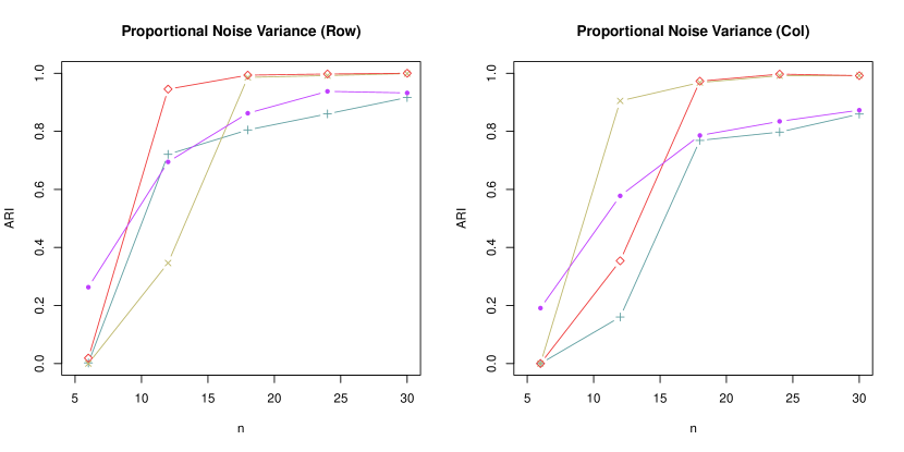
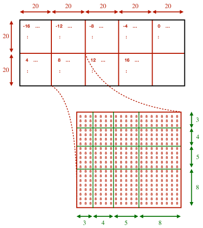
We consider the following data generating process. We fix , and a moderately unbalanced row and column cluster size structure (both having cluster sizes of , , , , , , , , , , respectively). This gives us the membership matrices and . The latent variable is generated from the matrix normal distribution , where and . We further generate , where we consider the following three settings for the noise variance: (1) homogeneous noise variances ; (2) heterogeneous noise variances proportional to the corresponding row and column cluster sizes: ; and (3) heterogeneous noise variances randomly generated from the Uniform distribution: where determines the level of heterogeneity. They will be referred to as the “homogeneous”, “proportional” and “random” cases, respectively.
Recall that in Section 3.1, the noise variances play an important role on the clustering consistency of our algorithm. We design these three settings to test the performance of our algorithm under different patterns of noise variances. We keep the mean noise variance to be 15 for all three cases. For the third setting, we set because it gives us a similar level of heterogeneity as the second setting. In both the second and third settings, the standard deviation of the noise variances is around 7.95. Finally, we generate from the model (1.1). We vary the sample size in the simulations and the simulations are repeated 30 times. To measure clustering accuracy, we consider the adjusted rand index (ARI) (Hubert and Arabie, 1985). Note that an ARI value of 1 implies a perfect match between the true and estimated cluster partitions. The formal definition of the ARI is shown in Section K of the Supplementary Material.
We consider the following clustering methods: (1) vanilla hierarchical; (2) Algorithm 1 with the initial weight (naive cod); (3) Algorithm 2 (1-step cod); and (4) Algorithm 3 (2-step cod in Section F.2 of the Supplementary Material). We emphasize that mean based clustering methods, such as K-means, cannot be used due to the centered nature of the data. This setting is indeed relevant as such data can be found in practice; see Section 8. As such, a competing method, vanilla hierarchical was constructed by applying agglomerative hierarchical clustering on a certain similarity matrix that utilizes covariance information in the data. For the rows, the average of the second moment of the columns of , , was used, and for the columns, the average of the second moment of the rows of , , was used. The silhouette method was used to estimate the optimal number of clusters for this competing method. In comparison, we note that the data-driven cross-validation scheme in Section F.4 was used to choose the tuning parameter in our cod based algorithms.
The competing method works decently as we tailored it to utilize correlation information, but is outperformed by the cod based methods when . It is apparent that perfect clustering is attained at a much smaller value with cod based methods compared to the competing vanilla hierarchical method.
In most cases, our iterative algorithms 1-step cod and 2-step cod improve the performance of naive cod, which is consistent with our theoretical analysis. In particular, 1-step cod and 2-step cod can achieve an ARI value close to 1 when , whereas naive cod may require much larger than to attain the same level of accuracy. The phenomenon holds for both row and column clustering. We also find that when is moderate (e.g., ), 1-step cod and 2-step cod have very similar performances. Due to the extra computational cost of 2-step cod, we generally recommend 1-step cod for practical use if is moderate or large. However if is small, 2-step cod may outperform 1-step cod.
We conducted additional simulation studies with other competing methods namely the model based tensor clustering methods deem, tgmm and temm in Mai et al. (2022) and Deng and Zhang (2022). The results and ensuing discussion can be found along with the main simulation results with different noise variance settings in Section I of the Supplementary Material.
8 Genomic Data Analysis
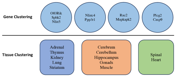
We apply our method to the atlas of gene expression in the mouse aging project dataset (Zahn et al., 2007), which contains gene expression values of 8932 genes in 16 tissues for 40 mice. Similar to Ning and Liu (2013) and Yin and Li (2012), we only focus on a subset of the data belonging to the mouse vascular endothelial growth factor signaling pathway. In order to maximize our usage of the tissue data, we drop 4 samples that have missing data for the tissues. So, in the end, our data is a array that corresponds to genes, tissues, and mice.
Figure 2 shows the gene clusters and tissue clusters obtained from our two-step Algorithm 3 with a data-driven tuning parameter. Disregarding the singletons - clusters with only one element - the estimated number of gene clusters is 4 and the estimated number of tissue clusters is 3. In Zahn et al. (2007), the authors group the tissues through hierarchical clustering, but they group genes that are similarly age-regulated through empirical meta analysis. Our method, on the other hand, can conveniently be applied to both the genes and the tissues at the same time. Interestingly, the tissue clustering result from our method agrees with the tissue clustering result in Zahn et al. (2007) which classifies tissues into 3 groups - vascular, neural, and steroid responsive. The “Cerebrum”, “Cerebellum”, and “Hippocampus” are all neural tissues that are parts of the brain, and they are all clustered into one tissue cluster by our algorithm. Also, “Adrenal” and “Thymus” tissues are steroid responsive tissues, while the “Lung” and “Kidney” tissues are vascular tissues. The respective pairs appear in our clustering result as well. As for gene clustering, it is known in the biology community that the O03Rik gene inhibits the Nfat5 gene. More specifically, O03Rik acts as a negative regulator of the calcineurin/NFAT signaling pathway and it inhibits NFAT nuclear translocation and transcriptional activity by suppressing the calcium-dependent calcineurin phosphatase activity (OriGene, 2020). It is then reasonable that the two genes are clustered together, because they would be highly negatively correlated. Also, calcineurin (Ppp3) is a serine/threonine protein phosphatase that is dependent on calcium and calcium modulated proteins (Hogan et al., 2003). It activates nuclear factor of activated T cell cytoplasmic (Nfatc), a transcription factor, by dephosphorylating it. This Nfatc happens to be encoded in part by the Nfatc4 gene. On the other hand, there are three isozymes of the catalytic subunit of calcineurin and this is encoded in part by the Ppp3r1 gene (Liu et al., 2005). Thus, the Ppp3r1 and Nfatc4 genes are both related to calcineurin - one having to do with how it is generated, and one having to do with something it activates. This reasonably explains the highly correlated results obtained from our clustering algorithm. Another possible explanation is given in Heit et al. (2006) which postulates that calcineurin/NFAT signaling is critical in -cell growth in the pancreas. All this external evidence suggests that our clustering results are biologically meaningful. We also have cluster results when applying a competing method DEEM (Deng and Zhang, 2022) on the same data. The cluster results along with a comparative discussion are presented in Section J of the Supplementary Material.
9 Discussion
In this paper, we study the variable clustering problem for matrix valued data under the latent variable model (1.1). A class of hierarchical clustering algorithms based on the weighted covariance difference is proposed. The theoretical and empirical performance of the algorithm heavily depends on the weight matrix . Theoretically, we show that under mild conditions, our algorithm with a large class of weight matrices can attain clustering consistency with high probability. To further characterize the effect of the weight matrix on the theoretical performance of our algorithm, we establish the minimax lower bound under the latent variable model (1.1), from which we prove that our algorithm using the weight matrix is minimax optimal for variable clustering. In particular, we apply the theory to the more concrete matrix normal model and show that clustering consistency and minimax optimality can be achieved in practice with an implementable initial weight, . Empirically, we develop iterative one-step and two-step algorithms based on the weight matrix , which outperform competing methods.
While we introduced extensions of our latent variable model and algorithms in Section 6, it would be interesting to further investigate each topic on its own. In particular, the theoretical effect of using different weight matrices when clustering higher order tensors with cod based methods would be an interesting direction. Another interesting extension would be to generalize our method to the overlapping clustering setting (Bing et al., 2020), where the rows and columns may simultaneously belong to multiple row and column clusters. For now, however, we leave them for future study.
Acknowledgment
Ning is supported in part by National Science Foundation (NSF) CAREER award DMS-1941945, NSF award DMS-1854637 and NIH 1RF1AG077820-01A1.
Supplementary Material
The supplement consists of additional technical details, derivations and discussions. Relevant proofs and additional numerical results are also included.
References
- Abbe (2017) Abbe, E. (2017). Community detection and stochastic block models: recent developments. The Journal of Machine Learning Research 18 6446–6531.
- Adamczak (2015) Adamczak, R. (2015). A note on the Hanson-Wright inequality for random vectors with dependencies. Electronic Communications in Probability 20 1 – 13.
- Airoldi et al. (2008) Airoldi, E. M., Blei, D., Fienberg, S. and Xing, E. (2008). Mixed membership stochastic blockmodels. Advances in neural information processing systems 21.
- Bai and Silverstein (2010) Bai, Z. and Silverstein, J. W. (2010). Spectral analysis of large dimensional random matrices, vol. 20. Springer.
- Basu and Michailidis (2015) Basu, S. and Michailidis, G. (2015). Regularized estimation in sparse high-dimensional time series models. The Annals of Statistics 43 1535–1567.
- Bing et al. (2020) Bing, X., Bunea, F., Ning, Y. and Wegkamp, M. (2020). Adaptive estimation in structured factor models with applications to overlapping clustering. The Annals of Statistics 48 2055–2081.
- Bunea et al. (2020) Bunea, F., Giraud, C., Luo, X., Royer, M. and Verzelen, N. (2020). Model assisted variable clustering: minimax-optimal recovery and algorithms. Annals of statistics 48 111.
- Cai et al. (2010) Cai, T. T., Zhang, C.-H. and Zhou, H. H. (2010). Optimal rates of convergence for covariance matrix estimation. The Annals of Statistics 38 2118–2144.
- Chi et al. (2017) Chi, E. C., Allen, G. I. and Baraniuk, R. G. (2017). Convex biclustering. Biometrics 73 10–19.
- Chi et al. (2020) Chi, E. C., Gaines, B. R., Sun, W. W., Zhou, H. and Yang, J. (2020). Provable convex co-clustering of tensors. The Journal of Machine Learning Research 21 8792–8849.
- Deng and Zhang (2022) Deng, K. and Zhang, X. (2022). Tensor envelope mixture model for simultaneous clustering and multiway dimension reduction. Biometrics 78 1067–1079.
- Eisenach et al. (2020) Eisenach, C., Bunea, F., Ning, Y. and Dinicu, C. (2020). High-dimensional inference for cluster-based graphical models. Journal of Machine Learning Research 21 1–55.
- Everitt et al. (2011) Everitt, B. S., Landau, S., Leese, M. and Stahl, D. (2011). Cluster analysis 5th ed. John Wiley.
-
Fraiman and Li (2022)
Fraiman, N. and Li, Z. (2022).
Biclustering with alternating k-means.
URL https://doi.org/10.48550/arXiv.2009.04550 - Hartigan (1972) Hartigan, J. A. (1972). Direct clustering of a data matrix. Journal of the american statistical association 67 123–129.
- Hastie et al. (2009) Hastie, Tibshirani and Friedman (2009). The Elements of Statistical Learning: Data Mining, Inference, and Prediction, Second Edition. Springer Series in Statistics, Springer.
- Heit et al. (2006) Heit, J. J., Apelqvist, Å. A., Gu, X., Winslow, M. M., Neilson, J. R., Crabtree, G. R. and Kim, S. K. (2006). Calcineurin/nfat signalling regulates pancreatic -cell growth and function. Nature 443 345–349.
- Hogan et al. (2003) Hogan, P. G., Chen, L., Nardone, J. and Rao, A. (2003). Transcriptional regulation by calcium, calcineurin, and nfat. Genes & development 17 2205–2232.
- Holland et al. (1983) Holland, P. W., Laskey, K. B. and Leinhardt, S. (1983). Stochastic blockmodels: First steps. Social networks 5 109–137.
- Hubert and Arabie (1985) Hubert, L. and Arabie, P. (1985). Comparing partitions. Journal of classification 2 193–218.
- Kogan (2007) Kogan, J. (2007). Introduction to clustering large and high-dimensional data. Cambridge University Press.
- Lee et al. (2010) Lee, M., Shen, H., Huang, J. Z. and Marron, J. (2010). Biclustering via sparse singular value decomposition. Biometrics 66 1087–1095.
- Li et al. (2010) Li, X., Ye, Y., Li, M. J. and Ng, M. K. (2010). On cluster tree for nested and multi-density data clustering. Pattern Recognition 43 3130–3143.
- Liu et al. (2005) Liu, L., Zhang, J., Yuan, J., Dang, Y., Yang, C., Chen, X., Xu, J. and Yu, L. (2005). Characterization of a human regulatory subunit of protein phosphatase 3 gene (ppp3rl) expressed specifically in testis. Molecular biology reports 32 41–45.
- Madeira and Oliveira (2004) Madeira, S. C. and Oliveira, A. L. (2004). Biclustering algorithms for biological data analysis: a survey. IEEE/ACM transactions on computational biology and bioinformatics 1 24–45.
- Mai et al. (2022) Mai, Q., Zhang, X., Pan, Y. and Deng, K. (2022). A doubly enhanced em algorithm for model-based tensor clustering. Journal of the American Statistical Association 117 2120–2134.
- Mankad and Michailidis (2014) Mankad, S. and Michailidis, G. (2014). Biclustering three-dimensional data arrays with plaid models. Journal of Computational and Graphical Statistics 23 943–965.
- Mitchell et al. (2008) Mitchell, T. M., Shinkareva, S. V., Carlson, A., Chang, K.-M., Malave, V. L., Mason, R. A. and Just, M. A. (2008). Predicting human brain activity associated with the meanings of nouns. Science 320 1191–1195.
- Ning and Liu (2013) Ning, Y. and Liu, H. (2013). High-dimensional semiparametric bigraphical models. Biometrika 100 655–670.
- OriGene (2020) OriGene (2020). 1500003o03rik (bc054733) mouse untagged clone. https://www.origene.com/catalog/cdna-clones/expression-plasmids/mc206143/1500003o03rik-bc054733-mouse-untagged-clone, [Accessed: 2021-9-17].
- Rand (1971) Rand, W. M. (1971). Objective criteria for the evaluation of clustering methods. Journal of the American Statistical association 66 846–850.
- Sill et al. (2011) Sill, M., Kaiser, S., Benner, A. and Kopp-Schneider, A. (2011). Robust biclustering by sparse singular value decomposition incorporating stability selection. Bioinformatics 27 2089–2097.
- Sun and Li (2019) Sun, W. W. and Li, L. (2019). Dynamic tensor clustering. Journal of the American Statistical Association 114 1894–1907.
- Tan and Witten (2014) Tan, K. M. and Witten, D. M. (2014). Sparse biclustering of transposable data. Journal of Computational and Graphical Statistics 23 985–1008.
- Vinh et al. (2009) Vinh, N. X., Epps, J. and Bailey, J. (2009). Information theoretic measures for clusterings comparison: is a correction for chance necessary? In Proceedings of the 26th annual international conference on machine learning.
- Wang et al. (2019) Wang, M., Fischer, J. and Song, Y. S. (2019). Three-way clustering of multi-tissue multi-individual gene expression data using semi-nonnegative tensor decomposition. The annals of applied statistics 13 1103.
- Wang and Zeng (2019) Wang, M. and Zeng, Y. (2019). Multiway clustering via tensor block models. Advances in Neural Information Processing Systems 32 715–725.
- Yin and Li (2012) Yin, J. and Li, H. (2012). Model selection and estimation in the matrix normal graphical model. Journal of multivariate analysis 107 119–140.
- Zahn et al. (2007) Zahn, J. M., Poosala, S., Owen, A. B., Ingram, D. K., Lustig, A., Carter, A., Weeraratna, A. T., Taub, D. D., Gorospe, M. and Mazan-Mamczarz, K. (2007). Agemap: a gene expression database for aging in mice. PLoS genetics 3 e201.
- Zhang et al. (2020) Zhang, Y., Levina, E. and Zhu, J. (2020). Detecting overlapping communities in networks using spectral methods. SIAM Journal on Mathematics of Data Science 2 265–283.
- Zhao et al. (2016) Zhao, H., Wang, D. D., Chen, L., Liu, X. and Yan, H. (2016). Identifying multi-dimensional co-clusters in tensors based on hyperplane detection in singular vector spaces. PloS one 11 e0162293.
Supplementary Material
Appendix A Comparison with the Vectorized Approach in Bunea et al. (2020)
Model (1.1) can be viewed as the extension of the G-block model for clustering a random vector in Bunea et al. (2020) to matrix valued data. If we vectorize the matrix , model (1.1) is equivalent to with , where denotes the vectorization of , formed by stacking the columns of into a single column vector, and denotes the Kronecker product. Thus, compared to Bunea et al. (2020) which allows to be any unstructured membership matrix, we impose the Kronecker product structure to the membership matrix . While our model for is more restrictive than Bunea et al. (2020), it actually comes with two advantages for matrix clustering. First, as seen above, and are interpreted as the membership matrices for the rows and columns. Ignoring the Kronecker product structure and directly applying the model in Bunea et al. (2020) would no longer produce interpretable results for matrix clustering, as shown in Figure 3. Second, the Kronecker product of and provides a more parsimonious parametrization for the unknown membership matrix , leading to stronger theoretical guarantees on clustering.
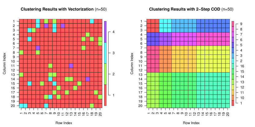
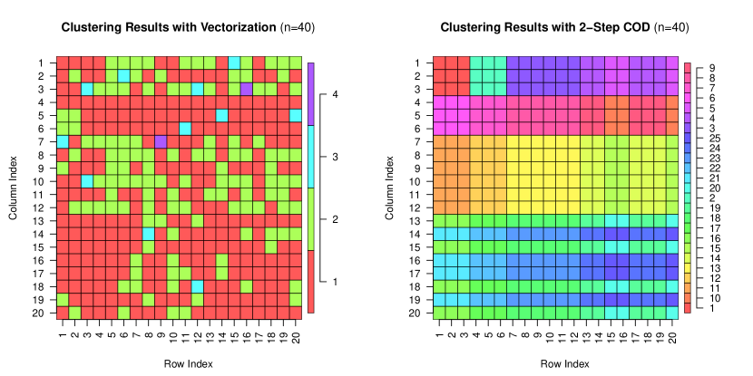
Appendix B Comparison of the Proposed Hierarchical Algorithm with the Algorithm in Bunea et al. (2020)
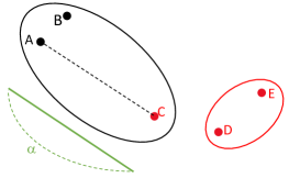
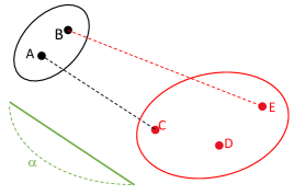
Like shown in Figure 4, if C,D,E have not been clustered yet and A and B are considered first, due to the nature of the algorithm in Bunea et al. (2020), since the distance between C and A is less than , C will be clustered with A and B even though C,D,E are closer to each other. If we implement a hierarchical approach, the distances between all the pairs of points will be considered at the same time, and a tree structure will naturally be constructed. The two groups of {A,B} and {C,D,E} will be formed in the \saylower part of the tree first, and even if the same threshold value is used, the two groups will not be merged together.
Appendix C Conditions for
In this section, we establish the conditions for for a general class of weight matrices. For brevity, we will discuss the row clustering case. Since our method is focused on using the columns to cluster the rows, we will focus on the class of weight matrices that are generated by arbitrary column membership matrices :
where is the number of clusters implied by . It can be shown that
where and denotes the smallest column cluster size implied by . So,
Note that when , then and the condition for is automatically satisfied. We expect that the condition is also satisfied for small perturbations , where .
Appendix D Derivation for Remark 3.2
We consider the setting where the column cluster has equal size (i.e., ) and . First, we have shown in Section 2.2 that the off diagonal entries of and are the same, that is . Then we have . For , we can show that
where is a constant. Hence, the cluster separation condition (A1) for is implied by
Similarly, the cluster separation condition (A1) for is implied by
In terms of the noise level , the condition for is , whereas the condition for is . The latter is clearly much weaker. Thus, when , our algorithm with the optimal weight attains clustering consistency in the presence of a larger noise level . This is the benefit of using the optimal weight in our algorithm.
Appendix E Minimax Lower Bound with a Perturbed
Here we present a lower bound result when the cluster separation metric in the definition of the parameter space is defined based on an arbitrary column membership matrix . For example, the special cases and are considered.
Assume that we have an arbitrary column membership matrix , which is fixed and can be different from the true membership matrix . Let where denotes the number of clusters implied by . We define the following parameter space
We now present a general lower bound for clustering over the parameter space .
Theorem E.1.
(Minimax Lower Bound with a Perturbed )
For , there exists a positive constant such that for any
| (E.1) |
we have
where denotes the smallest column cluster size implied by and . The infimum is taken over all possible estimators of .
This theorem shows that, if we define mcod based on a perturbed , the rate of the cluster separation (E.1) depends on and . If is near perfect, , , and in the construction of the lower bound. Then, , and will all be close to order and the bound in (E.1) becomes . In contrast, if we use , then is a matrix with row vectors as blocks on the diagonal. This implies that is a matrix with as square blocks in the diagonal, and in our construction. The lower bound becomes . These two cases show how the lower bound depends on the imperfect column cluster structure . The proof of this lower bound can be found in Section H.2.2 of the Supplementary Material.
Appendix F Supplementary Material for Section 5
F.1 Theoretical Guarantees for Algorithm 2
F.1.1 Consistency
We present the consistency theorem for the iterative one-step Algorithm 2 that clusters both the rows and the columns.
Theorem F.1.
(Consistency with One-step Hierarchical COD with the Optimal Weight)
Under the model , assume that is multivariate Gaussian, , and the following conditions hold:
-
(R)
Row Separation Condition:
where is an arbitrary constant and for a universal constant .
-
(C)
Column Separation Condition:
where is an arbitrary constant and for a universal constant .
-
(S)
Stability Condition:
where is defined in condition (R).
Then using our Algorithm 2 with the threshold for the row clustering step and the threshold for the column clustering step, we obtain perfect cluster recovery (i.e., and ) with probability greater than for some constant .
The row and column separation conditions (R) and (C) are similar to the cluster separation condition (A1) in Theorem 3.1. The stability condition (S) is only imposed for row clustering, which can be viewed as the condition for the initial value in Step 1 of Algorithm 2. As shown in Proposition 4.2, the initial value satisfies condition (S) under the matrix normal model with mild additional assumptions. Indeed, by Theorem 3.1, conditions (S) and (R) imply perfect row cluster recovery (i.e., ) with high probability, which further implies that . Thus, the stability condition for column clustering automatically holds, which in turn guarantees perfect column cluster recovery with high probability. The proof is very similar to the proof for Theorem 3.1 and will be omitted for brevity.
F.1.2 Minimax Optimality
In the following, we establish a lower bound result for both row and column clustering which naturally incorporates the uncertainty in estimating the membership matrices and simultaneously. Following the notation used in Theorem F.1, we define parameter spaces
and
for the rows and columns, respectively. To study the minimax lower bound for both row and column clustering, we consider the parameter space . The following theorem provides the lower bound for clustering over this parameter space .
Theorem F.2.
For , there exists a positive constant such that, for any and
we have
where the infimum is taken over all possible estimators of .
This theorem shows that we need and to attain both perfect row and column clustering. Together with Theorem F.1, we obtain that, as long as the initial estimate satisfies the stability condition (i.e., it falls into a contraction region), the One-Step Hierarchical Algorithm with the Optimal Weight (Algorithm 2) is minimax optimal for row and column clustering. Recall that this has been verified for the matrix normal model with in Proposition 4.2. Finally, we note that since the above lower bound is concerned with both row and column clustering, the uncertainty in estimating both membership matrices and is taken into account. The proof of this theorem is in Section H.2.3 of the Supplementary Material.
F.2 Two-Step Hierarchical Algorithm with the Optimal Weight
The two-step algorithm is shown in Algorithm 3. In this algorithm, we ignore the sample splitting step for simplicity.
-
(0a)
Set the initial value .
-
(0b)
Apply Algorithm 1 with to cluster the
Compute the estimate of the optimal column weight where is the estimated number of row clusters in . (1b) Apply Algorithm 1 with to cluster the columns
Compute the estimate of the optimal row weight ,
Apply Algorithm 1 with to cluster the rows
F.3 Simulation Results With and Without Sample Splitting
We present the results for an additional simulation study that highlights the difference of our method with and without sample splitting in Table 1. We have i.i.d. copies of matrices with and moderately unbalanced cluster sizes of for both the rows and columns. The decay rate for the Toeplitz covariance matrices is -0.2 and 0.2 for the rows and columns, respectively. We consider the proportional noise variance setting from the main paper. We vary from up to in increments of and the ARI values for 2-step cod are recorded. We see that, for relatively small (say ), our 2-step cod without data splitting performs significantly better than the method using data splitting. In addition, both methods yield very high clustering accuracy when is large enough (say ). Thus, in practice, we recommend using our 2-step cod without data splitting, especially when the sample size is small or moderate.
| Data Split (Row) | No Data Split (Row) | Data Split (Col) | No Data Split (Col) | ||
| 20 | 0 | 0.4984 | 0 | 0.2723 | |
| 40 | 0.0639 | 0.9939 | 0.0712 | 0.9562 | |
| 60 | 0.5642 | 1 | 0.1647 | 0.9979 | |
| 80 | 0.9685 | 1 | 0.6834 | 0.9934 | |
| 100 | 0.9849 | 1 | 0.9528 | 0.9962 |
F.4 Data-Driven Tuning Parameter Selection Process for
In the following, we describe a data-driven selection method for that was also used in Bunea et al. (2020). To fix the notation, we consider our Algorithm 1 with some sample covariance matrix . We assume the data are standardized. The method can be similarly applied to 1-step cod, 2-step cod with the optimal weight and naivecod. The steps are outlined in Algorithm 6.
We first split the data into two, , , and calculate , , respectively. For each tuning parameter in the grid, we perform our algorithm on to get a cluster structure . We then take the average of all the non-diagonal elements in the cluster blocks of via the smoothing operator . Finally we calculate the Frobenius loss of and , and choose that yields the smallest value.
-
1.
Split the data into two: and
-
2.
Using , calculate .
-
3.
Using , calculate .
-
4.
For and each value on a grid , perform Algorithm 1 with
Perform the smoothing operator where is defined as the following:
Our data dependent tuning parameter for the threshold is:
where is the Frobenius loss.
Appendix G Supplementary Material for Section 6
G.1 The Dependent Noise Model
G.1.1 Discussion of Theorem 6.1
Under model (1.1) with dependent noise elements, since , if ,
and if ,
where . In other words, is the counterpart to mcod that only considers the signal (the first component) from .
Comparing the population quantity in the two cases and , it is apparent that if the signal term is strong enough in the following sense
then even when the noise variables are dependent, the cod measures are well separated and on the population level, the cod method is still viable for clustering.
G.1.2 A Slightly Different Measure,
We can swap out the definition of in (6.1) for a slightly more restrictive but more intuitive defintion:
| (G.1) |
This can be used in place of the in the above theorem since the former is an upper bound for the latter. gives information on the largest off-diagonal entry in , i.e. the largest weighted covariance between two different noise variables. The relationship between this weighted covariance and the actual covariance between noise variables depends on the weight. For example, with the optimal weight , can be upper bounded with , where , the maximum of the unweighted covariance between two different noise variables.
G.2 Nested Clustering to Incorporate Mean Information
G.2.1 The Generalized Model
To generalize the proposed method to account for both mean and covariance information in clustering, we extend our latent variable model to
| (G.2) |
where , and are mean 0 random matrices. Like before, induces the row and column clustering structures based on the covariance of . Specifically, and are the unknown membership matrices for the rows and columns, respectively. We define the row clusters as
| (G.3) |
for any . The column clusters can be defined similarly. To incorporate the mean information, we further assume that the matrix induces the row and column clustering structures based on the mean of . In particular, we assume , where and are the unknown membership matrices for the rows and columns based on the mean information, and is an unknown deterministic matrix. The corresponding row clusters are defined as
| (G.4) |
for any . The column clusters can be defined similarly. To link these two row clusters and , we assume is nested inside .
Definition 1. (Li et al., 2010) A clustering with clusters is said to be nested inside another clustering with clusters if:
-
1.
(Hierarchical Structure) For any cluster , there is a cluster such that .
-
2.
(Proper Subset Structure) There exists at least one cluster in , (i.e. ), which satisfies and , for some cluster .
In other words, the clustering based on the covariance information provides a more refined partition on top of the initial clustering from the mean information. For the ease of interpretation, we only consider the case that is nested in . This assumption can be relaxed or even removed by defining clusters at different levels (e.g., clustering from the mean and covariance) and new ways of combining the clusters.
G.2.2 Nested Clustering (Algorithm 5)
To recover the nested cluster structure, we propose a two-step nested clustering algorithm, in which a mean-based clustering method is implemented first, and then on each cluster, our covariance-based method is applied to capture the finer, more intricate relationships within each broad cluster.
There are many existing mean-based clustering methods in the literature. Here we use SparseBC from Tan and Witten (2014) as the mean-based clustering method. The resulting clusterings are denoted by and . Then, our proposed two-step Algorithm 3 is implemented to get the second layer cluster structures within each first layer cluster. More specifically, for row clustering, we apply the two-step Algorithm 3 to each submatrix corresponding to the variables in for . Similarly, for column clustering, we apply our two-step Algorithm 3 to each submatrix corresponding to the variables in for . In this way, we can use mean information to reduce the dimension of the matrices, to which our two-step Algorithm 3 is applied. Thus, both the mean and the covariance information is utilized in deriving the final clustering result. We summarize this method in Algorithm 5.
-
(1)
Perform mean-based clustering (SparseBC) to get the first layer cluster structures and
-
(2a)
Perform Algorithm 3 on each submatrix
-
(2b)
Perform (the col. version of) Algorithm 3 on each submatrix
-
(3a)
Combine the row cluster results from each submatrix in (2a) to construct
-
(3b)
Combine the col. cluster results from each submatrix in (2b) to construct
G.2.3 Simulation Study Comparing Algorithm 3 and Algorithm 5
In order to illustrate the feasibility of this nested algorithm, we include simulation results with the aforementioned nested structure. For , we generate i.i.d. copies of a matrix () with two nested row clusterings and two nested column clusterings where the row clusterings are given by
The column clustering can be defined in a similar fashion, but for brevity it is omitted here. The true clustering can be visualized with Figure 5.
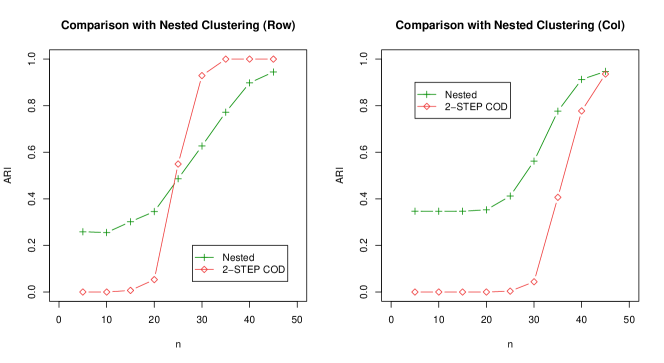
We use the ARI (Adjusted Rand Index, Vinh et al. (2009)) to compare the performance of the nested clustering method with our original 2-step cod method. The results are presented in Figure 6. Overall, considering the feature matrices are very large (), both methods work very well, as we get near perfect recovery once . Taking a closer look, for column clustering, the nested method is uniformly better than the original 2-step cod method over all values. For row clustering, for very small values of and , the nested method performs better, but for slightly larger values of and , the original 2-step cod method performs better. We observe that the closer the matrix is to a square, the easier it is for 2-step cod to cluster the rows and columns. If the matrix is highly unbalanced ( or ), then due to the iterative nature of 2-step cod (using rows to cluster columns, then using columns to cluster the rows, etc.), clustering one of the two dimensions becomes extremely difficult. This may lead to the final result being inaccurate. In our simulation settings, for row clustering, 2-step cod clusters over the entire matrix while the nested clustering method has to cluster over the two submatrices separately (if the mean-based clustering can perfectly recover ). This explains why the nested algorithm may perform worse than the original 2-step cod for row clustering.
We also implement the competing methods DEEM, TGMM and TEMM (Mai et al. (2022), Deng and Zhang (2022)), which are also included in the main simulation results, but none are able to be implemented successfully in this nested clustering simulation study. As explained in the main paper, their algorithms depend on different modeling assumptions and may fail to converge in our simulation setting.
All in all, we conclude that if the user wishes to incorporate mean information and also look at the finer clustering for the rows and columns that cannot be discerned by the mean alone, our cod based method can be used as the second step in a nested clustering type process (Algorithm 5) to obtain reliable results.
G.3 Higher Order Tensor Models
G.3.1 The Tensor Cluster Model and Algorithm 6
We present in the following the analog of our matrix clustering setting in a setting that is one order higher. Consider a three-way tensor . Assume that can be decomposed as
| (G.5) |
where is a three-way latent tensor (i.e., each entry of is a random variable) with , , and are the unknown membership matrices for the rows, columns and tubes of , respectively, and represents the mean 0 random noise tensor. Here, we use the -mode product notation from the tensor literature, e.g., is a tensor with . Similar to the matrix clustering setting, we assume the entries of are mutually independent and are also independent of . Each entry of the membership matrix takes values in , such that if row belongs to row cluster and otherwise. The membership matrices and are defined similarly. Assuming that i.i.d. samples of a random tensor are observed, our goal is to recover the membership matrices and .
Next, we define the so-called matricization (or equivalently, “unfolding”) of the tensor . Let denote the mode-1 matricization of , which arranges the mode-1 fibers of as columns into a matrix. Similarly, we can define and as the mode-2 and mode-3 matricizations of . Similar to the matrix clustering setting, we consider the weighted covariance matrix , where is some positive semi-definite weight matrix to be chosen. It is easily seen that exhibits the clustering structure for the rows, which can be identified via our cod algorithm. In particular, let for . The tensor clustering algorithm with the identity weight is shown in Algorithm 6. For simplicity, we only consider the identity weight. The algorithm may further be improved by using the optimal weight as in our one-step Algorithm 2 or our two-step Algorithm 3, but we leave the detailed analysis for future study.
-
for
-
-
Compute , where , and .
-
-
Apply Algorithm 1 to to construct , and , respectively.
-
-
G.3.2 Simulation Study
To illustrate the feasibility of our proposed method, we also conduct a simulation study with Algorithm 6 for which the results are presented in Table 2. We have i.i.d. copies of a tensor () that have Toeplitz covariance matrices in each direction with decay rates of -0.4, 0.3 and -0.2, respectively. The noise is generated in the homogeneous setting with the noise variance being to match our main simulation settings. It is seen that clustering is more accurate as the sample size grows, which provides empirical evidence for applying Algorithm 6 to higher-order tensors.
| Row (ARI) | Column (ARI) | Tube (ARI) | ||
| 10 | 0.0863 | 0 | 0.4449 | |
| 20 | 0.6637 | 0.3095 | 0.8904 | |
| 30 | 0.7594 | 0.7936 | 0.9334 | |
| 40 | 0.7864 | 0.8680 | 0.9033 | |
| 50 | 0.8107 | 0.8753 | 0.9889 |
While our preliminary simulation results are indeed promising, proving minimax optimality would be challenging in the tensor clustering. Also, as mentioned above, since using more intricate weight matrices instead of the identity matrix may improve the clustering performance, a rigorous analysis of the algorithm would also be interesting. All of these directions are promising fields of future study.
Appendix H Proofs
H.1 Clustering consistency
First, we state the Hanson-Wright inequality, which is instrumental in the proof.
Lemma H.1.
(Hanson-Wright) There exist positive constants such that for all matrices , if is a vector of independent mean 0 sub-Gaussian random variables with for some , then for all t, the following holds:
H.1.1 Proof of Theorem 3.1
Proof.
Denote and . So, . For simplicity, we assume , and the summation is from to . Furthermore, denote and . Denote . Since has mean 0 variance 1 given and is Gaussian, is a vector of independent Gaussian random variables given .
Denote
| and | ||
where and each have blocks on the diagonal. Note that the quadratic forms can be used to get the sum of the products. The following calculation holds for one observation:
We can extend this to observations by using block matrix notation from above.
Thus, we have
By Lemma H.1, we know that there exist positive constants such that: conditioned on with probability greater than ,
Similarly, conditioned on with probability greater than ,
By the definition of , we know and . Thus, with a union bound over , we get the following concentration inequality:
| (H.1) |
conditioned on with probability greater than , and setting , we know the inequality (H.1) holds with conditional probability greater than . By taking another expectation with , the inequality (H.1) holds with probability greater than unconditionally.
Because holds in general, the Frobenius term dominates in the regime of , so all that is left to do is to bound . An identical argument can be made for , and we know the following upper bound holds for both terms,
This holds for all pairs , and so it also holds for the maximum over the pairs:
| (H.2) |
Thus, with probability greater than ,
| (H.3) |
for some constant , where the last step is from condition (A1).
Note that conditions (A1) and (A2) together imply that
| (H.4) |
In the following, we show how perfect clustering is achieved under the event that the inequality (H.3) holds. For simplicity, we drop the subscript in and and just write and . Also, for simplicity, in the following derivation, we will denote the -th element of as . Define the following quantity
Then we have:
where the last step is from (H.3). We now want to show the following inequality:
| (H.5) |
The inequality on the left holds because of the following:
| (H.6) |
With a similar technique, we can get the inequality on the right as well. Now, for any two sets and , if and indeed belong to the same cluster (i.e., for some and for any and ), we have and therefore by (H.5)
If and are not the same clusters, there must exist and with and for some . Then
where the first inequality is from the definition of , the second one is from (H.5), the third one is from the definition of mcod, and finally the last one is from (H.6).
Together with (H.4), finally we show that , if and are not the same clusters. By taking the threshold value , we attain perfect clustering using our hierarchical algorithm. This completes the proof. ∎
H.2 Minimax Lower Bound
The following lemma is Birge’s Lemma applied to our specific setting, similar to Lemma C.1 in Bunea et al. (2020). Define as in Section 3.2. For ease of notation, we will simply use .
Lemma H.2.
For any partition estimator , and for any collection of distinct covariance matrices ,
H.2.1 Proof of Theorem 3.2
Similar to the construction in Bunea et al. (2020), set our collection of covariance matrices as follows: (equal row cluster size), , where has entries where denotes the noise variance of elements in column cluster . Note that for this construction, we assume the same noise variance within the same column cluster. In addition, we set
where is a quantity to be specified later. We will consider many covariance matrices that are obtained by switching one of the rows in the first third of the rows in and one of the rows in the second third of the rows in (and also counting the original matrix as well).
It follows that and that
So we can set as one of the () blocks in the block diagonal matrix .
Note that the Kullback-Leibler Divergence for iid multivariate normal observations in with mean is , where and are two covariance matrices constructed as above. Thus, since is a block diagonal matrix with blocks , we have the relationship , and it suffices to just calculate in order to calculate .
Denote the eigenvalues and eigenvectors of as and , respectively. Also, define the vector as .
where we note that . Therefore,
Let denote a perturbation matrix switching one row in the first third of the rows in and one row in the second third of the rows in . Define . Then holds. Now, set . It follows that
Then we can calculate :
where the last equality holds because . Now we compute in the following way:
where the second to third line holds because and the last line holds from
where and . Note that the two non-zero eigenvalues of , which are , and , satisfy and . Using these facts, we can finally calculate the KL divergence
where the last equality holds because . Now, plugging in , we get:
where we use the fact that . Thus,
| (H.7) |
In the following, we will show an lower bound for the rate of . We will first compute ,
and from the definition of , it is apparent that the minimum of the maximum difference between rows is , that is
| (H.8) |
Let us choose
| (H.9) |
The choice of will be explained later.
Furthermore, we can show that
So, getting rid of the term , and using in (H.9) and , , we get the following inequalities:
where for our construction we use the noise variance setting of in the last equality. This ensures that the lower bound is as tight as possible. This implies that our constructed belongs to the parameter space for some s.t. .
H.2.2 Proof for Theorem E.1 (Minimax Lower Bound with a Perturbed )
Proof.
To study the lower bound over , we follow the same construction as in the proof for Theorem 3.2. We emphasize that all the parts leading up to calculating the KL - divergence is the same regardless of the value of as the KL-divergence is related to the model on the population level. Since the true column clustering structure does not change, the derivations up to this point remain unchanged. The part that does indeed change is the calculation of as both the MCOD value and depend on . We can show that
where . Thus
Thus, we have
where the is from our construction. Note that all of the entries of are non-negative and all the column sums are 1. Thus, every entry in is , and the entries in add up to . We can conclude that . Thus, . It is apparent that the mcod value potentially decreases with a weight with an incorrect estimated column cluster structure. When , then and , and the mcod value reduces to . Also, when , then , , and the mcod value reduces to as well. It appears that these two are the exception, as in other cases, the mcod value becomes strictly smaller than . For example, when (when we put all the columns in the same column cluster) we have , and which is strictly smaller than 1. The mcod value becomes .
Now let’s look at :
| (we can take the maximum diagonal value in .) | |||
| where denotes the r-th estimated column cluster and | |||
| since we assume in our construction | |||
| where denotes the smallest estimated column cluster size |
Finally, we can derive the lower bound rate for :
| since we assume in our construction. |
This completes the proof of the lower bound. ∎
H.2.3 Proof of Theorem F.2 (Joint Lower Bound)
Proof.
The extension from considering just one direction (either the rows or columns) is quite trivial.
where the last line holds from the minimax lower bound construction for Theorem 3.2. The only thing left to check for the proof is that the constructed in the previous minimax lower bound proof is actually an element of both parameter spaces - and - so that the supremum logic is valid. We will show that the constructed in the minimax lower bound proof for the row clusters also satisfies for . We have
| (Note the columns of are independent in our construction.) | |||
| (Again, from column independence of in our construction.) | |||
We have shown that the constructed for the minimax lower bound proof for the rows is also an element of . The same argument can be made symmetrically to show that the constructed for the minimax lower bound proof for the columns is also an element of . Thus, the proof for joint minimax optimality is complete. ∎
H.3 Proofs for the Matrix Normal Model
H.3.1 Proof of Proposition 4.1
Proof.
For any rows of , without loss of generality, we can assume they belong to clusters . Then
Looking at the cluster separation condition first, we need this cod value to be greater than for all (where is a universal constant and is an arbitrary constant .). We know that from the definition of . In the matrix normal setting, we have
and so, and we have
It is also easily shown that
Rearranging with algebra gives us the cluster separation condition.
Now, let’s consider the stability condition. Again, we need only consider rows in different row clusters when looking at the mcod value. That is why we assume . Now for , we would need to look at the following equivalent expressions:
where for simplicity we drop the upperscript in and .
Note that both and are influenced by and () only through the common term, and so the pair that gives the minimum of the two cod expressions is the same. Thus, the following holds:
Thus,
needs to hold. By Von Neumann’s trace inequality, we have , and so it suffices to have:
To show the above inequality, we need to further lower bound ,
For the term in the denominator, we have
| (H.10) | ||||
| (H.11) | ||||
where (H.10) holds from the fact that , and (H.11) holds from the fact there can be at most min non-zero eigenvalues of because rank() min{rank(), rank()} and rank() min(). Using the similar argument, we also show that
Finally, noting that , and
we have
So, combining with the above inequality, we need to show the following condition:
| (H.12) |
To show (H.12), let’s consider the following two cases.
If holds, then
when . In the second case , we can similarly show that
when . This completes the proof. ∎
H.3.2 Proof of Proposition 4.2
Proof.
Recall that our definition of from Section 4 is as follows:
Note that when . It is easily seen that (up to order) where denotes the -th smallest column cluster size. Thus, and , where and denote the smallest and largest column cluster sizes, respectively.
Recall we have defined:
Under the assumption that the noise is homogeneous and the cluster size is balanced (i.e., for all , , for some constant ), we have that . Also, by the formulation of our weight , we have that .
In order to satisfy the stability condition in Proposition 4.1 (which is the condition related to the effect of the initial weight), when using , the second set of conditions, (ii), is more relaxed. These conditions are implied by the following:
Assuming that is a constant, the latter condition will hold as long as we take a large enough value. Recall this is an arbitrary constant that determines the tradeoff between separation and stability. As for the former condition, since , we have . Thus, as long as , the first condition is satisfied. ∎
Appendix I Additional Simulations
I.1 Main Simulation Results with Alternative Noise Settings
The results for the entire main simulations including the homogeneous and random noise variance settings are shown in Figure 7. The implications from the different settings are very similar and will be omitted here for brevity.
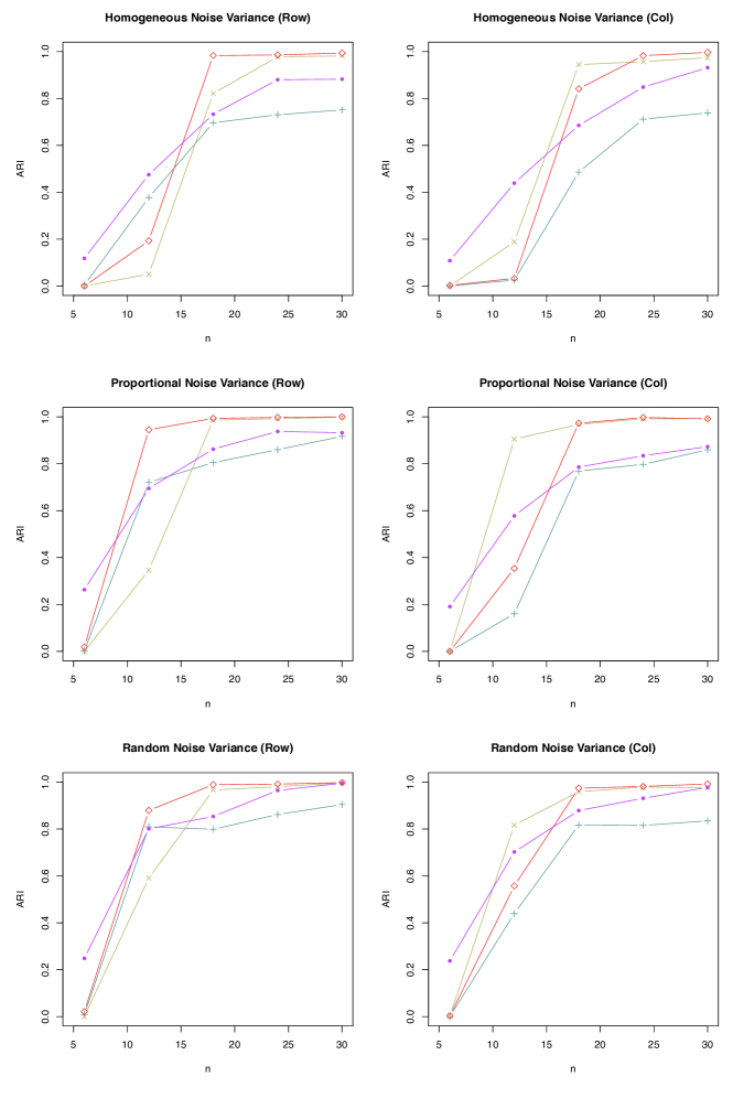
I.2 Comparison with DEEM, TGMM and TEEM
In this section, we consider for comparison the following clustering methods: (1) DEEM; (2) TGMM; (3) TEMM; (4) Algorithm 1 with the initial weight (naive cod); (5) Algorithm 2 (1-step cod); and (6) Algorithm 3 (2-step cod in Section F.2 of the Supplementary Material). We note that the data-driven cross-validation scheme is used to choose the tuning parameter in our cod-based algorithms. The competing methods we used in our simulations came from recent model based tensor clustering papers, Mai et al. (2022) and Deng and Zhang (2022). Their DEEM and TGMM methods utilize the tensor normal mixture model and their TEMM method utilizes the tensor envelope mixture model. Together with some variants of the EM algorithm, the authors exploited not only the mean information, but also the covariance structure in each direction of the tensor. These methods were implemented in our simulations using their designated functions within the R package TensorClustering.
Since the goal of DEEM, TGMM and TEMM is to cluster over i.i.d copies of tensors rather than the features, we need to adapt their methods for row and column clustering in our simulations. In particular, we implement row clustering by regarding the rows in our setting to be the direction of the observations in their tensor setting, and regard our matrix slices to be the tensors in their tensor setting. Note that this violates their tensor normal distributional assumptions as the “copies” of matrix slices are no longer i.i.d. The column clustering is performed similarly. The simulation results for the random noise variance setting are shown in Figure 10. The results for the other two noise variance settings can be found in Section I.1 of the Supplementary Material.
It must be noted that since the distributional assumptions for the DEEM, TGMM and TEMM methods are violated, these methods fail to converge in some of the runs, especially when is large. One possible reason is that when is larger, the i.i.d. assumption is more severely violated and the computation becomes indeterminate in the process. In order to fairly compare our method with DEEM, TGMM and TEMM, we report not only the average ARI among the successful runs of their methods, but also the percentage of the successful runs out of the total number of runs. The latter is called the “successful implementation rate”.
I.2.1 Balanced and
We consider the following data generating process. We fix , and a moderately unbalanced row and column cluster size structure (both having cluster sizes of , , , , , , , , , , respectively). This gives us the membership matrices and . The latent variable is generated from the matrix normal distribution , where and . We further generate , where we consider the following three settings for the noise variance: (1) homogeneous noise variances ; (2) heterogeneous noise variances proportional to the corresponding row and column cluster sizes: ; and (3) heterogeneous noise variances randomly generated from the Uniform distribution: where determines the level of heterogeneity. They will be referred to as the “homogeneous”, “proportional” and “random” cases, respectively.
The simulation results show that in all three noise variance settings the successful implementation rates of DEEM, TGMM and TEMM decrease drastically as increases. In contrast, our cod methods never fail to converge in any of the settings. When the competing methods converge, the ARI is decent, especially when where they outperform the cod methods in the homogeneous and random noise variance settings. However, as grows, our cod methods become more reliable and more accurate.
In most cases, our iterative algorithms 1-step cod and 2-step cod improve the performance of naive cod, which is consistent with our theoretical analysis. In particular, 1-step cod and 2-step cod can achieve an ARI value close to 1 when , whereas the naive cod may require much larger than to attain the same level of accuracy. The phenomenon holds for both row and column clustering. We also find that when is moderate (e.g., ), 1-step cod and 2-step cod have very similar performances. Due to the extra computational cost of 2-step cod, we generally recommend 1-step cod for practical use if is moderate or large. However if is small, 2-step cod may outperform 1-step cod.
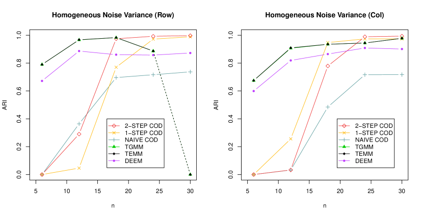
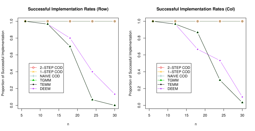
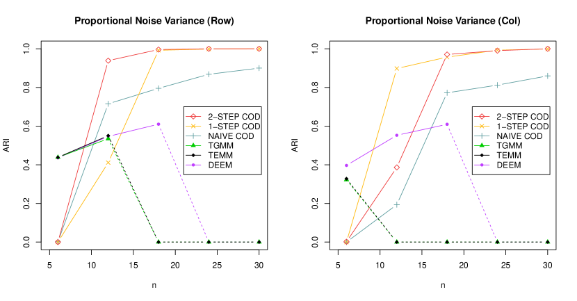
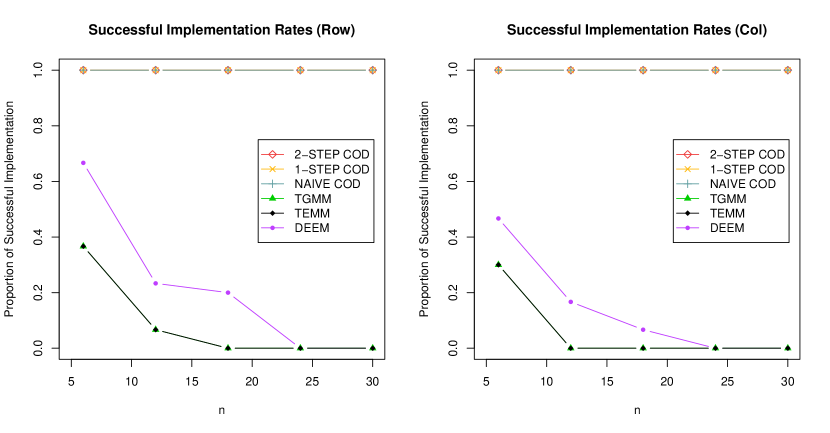

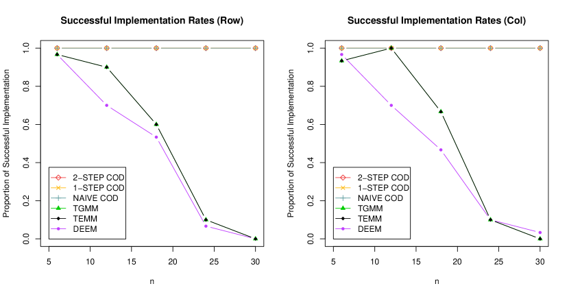
I.2.2 Unbalanced and
Here we present the unbalanced setting of , , , (with all of the other settings being the same as in I.2.1) shown in Figures 11, 12 and 13. In this case, we have long, skinny matrices that are “unbalanced”. We find that the cod methods perform drastically better in column clustering compared to the tensor model based methods. In all three noise variance settings, the competing methods have 0 successful implementation rates across all values in column clustering, whereas our cod methods perform significantly better. We believe this occurs because in the tensor normal setting, having too small of a value is equivalent to having too few “i.i.d. observations”, which causes their algorithms to diverge. In contrast, for the cod algorithms, since the threshold for perfect column clustering recovery is on the order of , if is relatively small and is relatively large, this threshold decreases compared to the balanced matrix setting and the condition for perfect column clustering recovery becomes more relaxed. Thus, our cod based methods typically yield more accurate clustering results compared to the competing tensor model based methods, especially when the number of rows and columns are unbalanced.
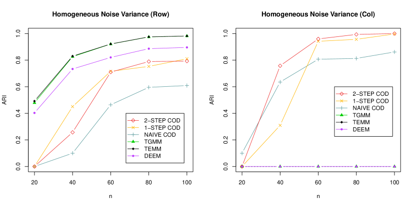
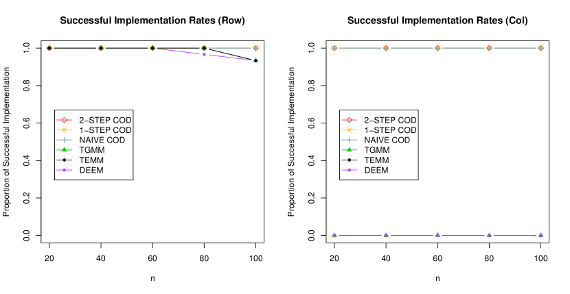
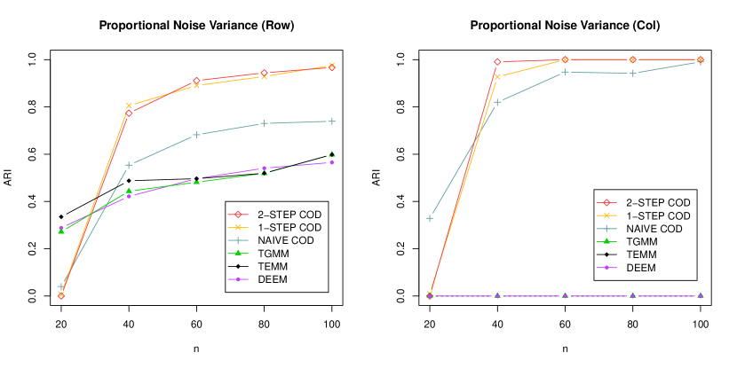
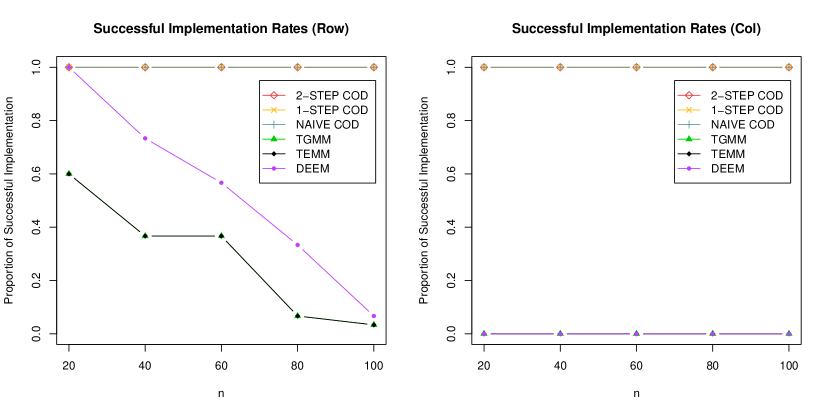
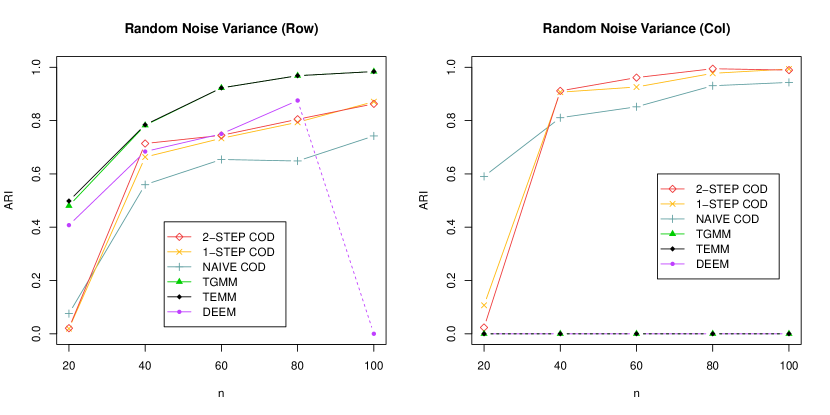
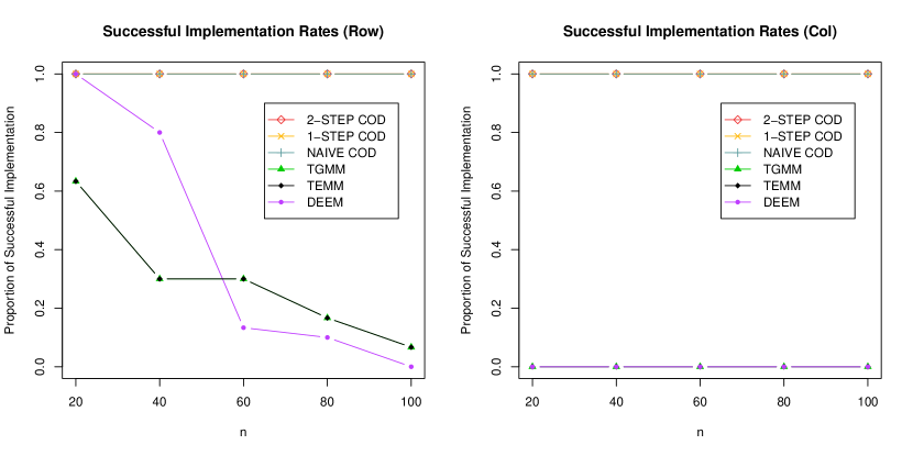
Appendix J Real Data Analysis with a Competing Method
We add the real data analysis results from using the competing method DEEM (Deng and Zhang (2022)) on the same gene-tissue data mentioned in Section 8. The results are illustrated in Figure 14. Of the gene clustering results from our method shown in Figure 2, DEEM was also able to cluster “O03Rik” and “Nfat5” together and “Rac2” and “Mapkapk2” together. However, DEEM was not able to capture the relationship between “Nfatc4” and “Ppp3r1”, which was identified with our method. The mechanism behind the relationship is that the “Ppp3r1” and “Nfatc4” genes are both related to calcineurin - one having to do with how it is generated, and one having to do with something it activates. Another possible explanation is given in Heit et al. (2006) which postulates that calcineurin/NFAT signaling is critical in -cell growth in the pancreas. Either way, it signals that our method can cluster meaningful genes that are not able to be identified with other competing methods. For the tissues, the competing method DEEM was able to cluster the “Lung” - “Heart” pair of vascular tissues and the “Adrenal” - “Gonads” pair of steroid responsive tissues that did not appear in our results with cod. However, it was not able to cluster the “Cerebrum” - “Cerebellum” - “Hippocampus” trio of neural tissues, the steroid responsive “Adrenal” - “Thymus” pair, or the vascular “Lung” - “Kidney” pair that were clustered together with cod. Thus, although the competing method gives reasonably meaningful results that are different from the results using cod, it is apparent that our method can complement existing clustering methods and provide useful information that wasn’t available.
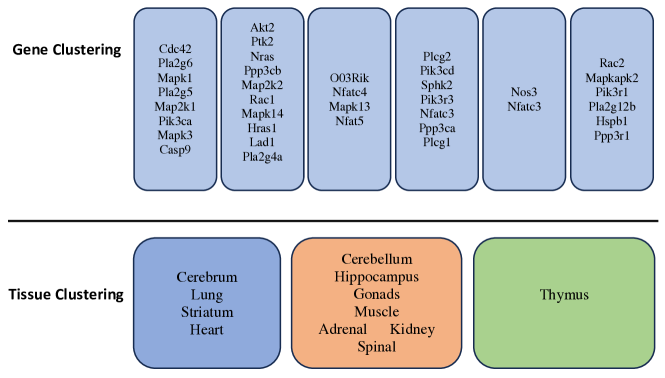
Appendix K Cluster Evaluation Metrics
For this section, the true row cluster partition will be denoted simply as
, while the estimated row cluster partition will be denoted as .
K.1 Sensitivity and Specificity
Then, for any pair , we can define
and define
Sensitivity (SN) and specificity (SP) can then be defined as follows:
K.2 Adjusted Rand Index (ARI)
The following is a cross tabulation of two cluster partitions (the true partition and the estimated partition).
| … | Sum | ||||
| … | |||||
| … | |||||
| : | : | : | … | : | : |
| … | |||||
| Sum | … |
The ARI is then defined as follows:
Note that this is the corrected-for-chance version of the Rand index (Rand, 1971). An ARI value of 1 implies a perfect match between the two cluster partitions.