Annealed Leap-Point Sampler for Multimodal Target Distributions

Abstract

In Bayesian statistics, exploring multimodal posterior distribution poses major challenges for existing techniques such as Markov Chain Monte Carlo (MCMC). These problems are exacerbated in high-dimensional settings where MCMC methods typically rely upon localised proposal mechanisms. This paper introduces the Annealed Leap-Point Sampler (ALPS), which augments the target distribution state space with modified annealed (cooled) target distributions, in contrast to traditional approaches which have employed tempering. The temperature of the coldest state is chosen such that its corresponding annealed target density can be sufficiently well-approximated by a Laplace approximation. As a result, a Gaussian mixture independence Metropolis-Hastings sampler can perform mode-jumping proposals even in high-dimensional problems. The ability of this procedure to mode hop at this super-cold state is then filtered through to the target state using a sequence of tempered targets in a similar way to that in parallel tempering methods. ALPS also incorporates the best aspects of current gold-standard approaches to multimodal sampling in high-dimensional contexts. A theoretical analysis of the ALPS approach in high dimensions is given, providing practitioners with a gauge on the optimal setup as well as the scalability of the algorithm. For a $d$-dimensional problem the it is shown that the coldest inverse temperature level required for the ALPS only needs to be linear in the dimension, $\mathcal{O}(d)$, and this means that for a collection of multimodal problems the algorithmic cost is polynomial, $\mathcal{O}\left(d^{3}\right)$. ALPS is illustrated on a complex multimodal posterior distribution that arises from a seemingly-unrelated regression (SUR) model of longitudinal data from U.S. manufacturing firms.

1 Introduction

The standard approach to sampling from a multivariate Bayesian posterior density known up to a constant of proportionality is Markov Chain Monte Carlo (MCMC). There is a wealth of established literature and methodology enabling the construction construct of a Markov chain with prescribed invariant distribution, e.g., Robert and Casella (2013). Arguably the easiest way to construct such a chain is by using localised proposals and creating a reversible chain by accepting or rejecting according to the Metropolis-Hastings acceptance probability, (Hastings, 1970).

When the target exhibits multimodality then the majority of MCMC algorithms which use localised proposal mechanisms e.g., Roberts et al. (1997), Roberts et al. (2001), Mangoubi et al. (2018), fail to explore the state space leading to biased sample output. Indeed, when the target distribution is high-dimensional or the posterior from a complex Bayesian modeling context then it becomes very hard to know if the posterior is multimodal. Therefore it is important to develop methods that are robust but also scale well to high-dimensional settings.

This paper introduces a new algorithm, the Annealed Leap Point Sampler (ALPS), that is designed to sample from a class of smooth densities on $\mathbb{R}^{d}$ that may exhibit multimodality. The ALPS construction uses an annealing approach as opposed to the traditionally used tempering approaches. It also adapts additional ideas from established methods in the literature designed to mitigate the worst effects of multimodality in multi-dimensional settings. As well as presenting novel methodology, this paper introduces accompanying theoretical results that describe its computational complexity (under suitable regularity) and which underpin practical guidance on temperature selection for the algorithm. The conclusion is that the coldest inverse temperature $\beta_{\text{max}}$ should be selected so that it scales as $\mathcal{O}(d)$ resulting in a computational cost of $\mathcal{O}\left(d^{3}\right)$.

The merits of the ALPS procedure are demonstrated empirically firstly on a very complex synthetic example and then on a highly-complex and previously unsolved problem, a Seemingly-Unrelated Regression (SUR) model for manufacturing investment data Grunfeld (1958). SUR models were introduced by Zellner (1962) and are widely used for panel data in econometrics. Many examples are provided by Srivastava and Giles (1987) and Fiebig (2001). It has only relatively recently been established that the SUR model likelihood exhibits multimodality and that the current methodology for inference is not robust. It is shown that ALPS can successfully overcome the difficulties in both the synthetic problem as well as the complex real-data SUR model setting.

The paper is structured as follows: Section 2 outlines the procedure for ALPS; Section 3 presents the details of the components of the algorithm; Section 4 presents the main theoretical contribution of the paper that is crucial to understanding the computational cost of the procedure; Section 5 discusses the computational cost and how it scales with the dimension of the problem; Section 6 contains empirical studies; and Section 7 presents our conclusions and considerations for further work.

1.1 ALPS Motivation

There is a wealth of literature focused on overcoming the multimodality problem; the methods can be roughly designated into one of two approaches. The first collection of approaches uses “mode jumping” proposals, e.g. Tjelmeland and Hegstad (2001), Ibrahim (2009), Liu et al. (2000), Tjelmeland and Eidsvik (2004) and Pompe et al. (2020). There is typically no explicit state space augmentation with such methods. The second collection appeal to state space augmentation methods. These augmentation approaches typically use auxiliary target distributions that allow a Markov chain to efficiently explore the entire state space and use the resulting rapid mixing information to aid the mixing in the desired target, e.g. Wang and Swendsen (1990), Geyer (1991), Marinari and Parisi (1992), Neal (1996), Kou et al. (2006), Nemeth et al. (2017) and Tawn and Roberts (2019).

Both classes of approaches have their strengths and weaknesses. Part of the motivation for the novel methodology presented in this paper is to design an algorithm that combine their strengths while mitigating as many of their weaknesses as possible.

Consider the problem of sampling from a $d$-dimensional smooth density function $\pi(\cdot)$ which is known (or suspected) be be multimodal. One of the gold standard approaches to this problem is the parallel tempering (PT) algorithm, Geyer (1991). The principle is that a Markov chain can achieve global exploration when targeting a tempered version ($\pi^{\beta}$ for some $0<\beta<1$). However, despite its many successes, there are some negative results regarding the algorithm’s performance in high-dimensional settings, e.g. Woodard et al. (2009a), Woodard et al. (2009b) and Bhatnagar and Randall (2016). There have been recent developments in Tawn et al. (2020), Tawn and Roberts (2018) and Tawn and Roberts (2019) that accelerate the performance of PT. However, these approaches lack robustness when the modes of the target distribution exhibit significant skewness and heterogeneous scale.

Tawn et al. (2020) attempts to address the issues of heterogeneous scale, by tempering applied in a localised way. However, there remain questions over the high-dimensional practicality of the approach, especially regarding the Markov chain’s convergence properties for the tempered target distributions that are essential to ensuring successful global exploration.

Alternative approaches, e.g. Tjelmeland and Hegstad (2001) and Ibrahim (2009), attempt to approximate the target distribution via local Laplace approximations in order to design appropriate inter-modal MCMC moves. However, their mixing times increase exponentially in dimension, Liu (1996). Performance is particularly problematic where the modes of the target distribution exhibit skewness. Even in one dimension, the best Gaussian mixture approximation to the target distribution might not be a good fit, see for example Figure 1 (c).

Overcoming these problems and developing a practically applicable algorithm is the motivation behind this work. The most significant novelty in this work is that an annealing approach (i.e.  $\beta>1$) is adopted to reduce the skew of any particular mode, making it appear approximately Gaussian. From Figure 1 (a) and (b) we can clearly see the effect of reducing skew by annealing. This greatly facilitates the design of a Markov chain that has efficient inter-modal mixing properties (in practice we use a mode-hopping independence Metropolis Hastings sampler).

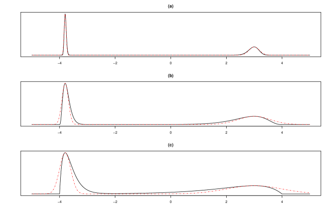
Figure 1: Annealing help to reduce skew. Figure (c) shows a bimodal density with appreciable skewness. Figures (b) and (a) show annealed versions of the density. Gaussian mixtures are superimposed in red showing that the fit improves as annealing is increased.

We shall show that this ambitious plan can be accomplished by giving detailed methodology and supporting theory that demonstrates its robustness in high dimensional contexts. In particular we shall see that this annealing approach can be carried out without an increase in computational complexity in comparison to standard tempering methods.

2 The ALPS Algorithm

ALPS constitutes two parts, the Parallel Annealing (PA) which is an annealing “parallel tempering” scheme and ”Exploration Component” (EC) which is a procedure aimed at exploring the whole state space to identify the location of modes. These two processes run in parallel with the information from the exploration component being used to adapt both the target distribution and the proposal mechanism to ensure effective global mixing.

With the $d$-dimensional target distribution denoted by $\pi(\cdot)$, the following notation is introduced.

• $M:=\{\mu_{1},\ldots,\mu_{m}\}$, the collection of mode points of the $\pi$, with $m$ is the number of unique mode points discovered by iteration $t$;

• $S:=\{\Sigma_{1},\ldots,\Sigma_{m}\}$, where $\Sigma_{i}=-\left[\nabla^{2}\log(\pi(\mu_{i}))\right]^{-1},\leavevmode\nobreak\ \leavevmode\nobreak\ i=1,\ldots m_{t}$ again using $m$ to denote the number of modes discovered by iteration $t$ of the procedure;

• $W=\{\hat{w}_{1},\ldots,\hat{w}_{m}\}$, the collection of approximated weights

  $$\hat{w_{j}}=\frac{\pi(\mu_{j})|\Sigma_{j}|^{1/2}}{\sum_{k=1}^{m}\pi(\mu_{k})|\Sigma_{k}|^{1/2}},\leavevmode\nobreak\ \leavevmode\nobreak\ j=1,\ldots,m_{t}$$ (1)

• $\Delta=\{\beta_{\text{hot}},\beta_{0},\beta_{1},\ldots,\beta_{n}\}$, the tempering schedule, which determines a sequence of auxiliary probability densities. $\Delta$ includes the inverse temperature used in the EC, $\beta_{\text{hot}}\in(0,1)$ as well as the inverse temperature schedule for PA of the algorithm where $1=\beta_{0}<\ldots<\beta_{n}:=\beta_{\text{max}}$;

• $Q:=\{q_{\beta_{\text{hot}}}(\cdot,\cdot),q_{\beta_{0}}(\cdot,\cdot),\ldots,q_{\beta_{n}}(\cdot,\cdot)\}$, a collection of proposal distributions to undertake the temperature-marginal MCMC updates for the augmented target given below in (2);

• $P_{\beta_{j}}(\cdot,\cdot)$ the transition kernel for the MCMC move with associated proposal density $q_{\beta_{j}}(\cdot,\cdot)$ updating the $\beta_{j}$ inverse temperature marginal component.

The ALPS algorithm constructs a Markov chain on the space $\mathbb{R}^{d(n+2)}$, whose value at iteration $t$ is denoted by $X^{t}:=(x_{\text{hot}}^{t},x_{0}^{t},\ldots,x_{n}^{t})$, which is targeting the invariant distribution

$$\pi_{ALPS}(X)\propto\left(\pi\left(x_{\text{hot}}\right)\right)^{\beta_{\text{hot}}}\prod_{j=0}^{n}\pi_{\beta_{j}}(x_{j}),$$ (2)

where the targets denoted by $\pi_{\beta_{j}}$ are defined in Section 3.1.

With the specified notation the outline of the ALPS procedure is given in Algorithm 1 with reference to the details of the steps in the following Sections 3.1, 3.2 and 3.3.

The $\pi_{\beta_{j}}$ marginal targets adapt their form through a burn-in phase of the Markov chain as the EC discovers mode location information. There are no guarantees on the EC finding all modes in a finite run of the algorithm but in an example with a finite number of modes, one expects the adaptation to take a finite amount of time.

Algorithm 1 The Annealed Leap Point Sampler (ALPS)

1:Collections $\Delta$ and $Q$ given above along with initial mode point information $I^{0}:=\{M^{0},S^{0},W^{0}\}$; initialising chain values, $X^{0}=\{x_{0}^{0},x^{0}_{1},\ldots,x^{0}_{n}\}$; a within temperature proposal mechanism, $q_{\beta}(x,\cdot)$; $N$, the number of algorithm iterations; $L$ the cut-off level for using the the transformation-aided temperature swap move and $v$, the number of within-temperature moves and $s$ the number of temperature swaps.

2:procedure ALPS($X^{0}$)

3:     for $i\leftarrow 1\textrm{ to }N$ do

4:         Parallel Annealing:

5:         $t$ $\leftarrow$ $(i-1)+(i-1)(m+1)$

6:         Temperature-Marginal Chain Updates:

7:         for $j\leftarrow 0\textrm{ to }(n-1)$ do

8:              for $l\leftarrow 1\textrm{ to }v$ do

9:                  Update: $x_{p}^{t+l}\sim P_{\beta_{j}}(x_{p}^{t+l-1},\cdot)$

10:              end for

11:         end for

12:         for $k\leftarrow 1\textrm{ to }v$ do

13:              $\beta_{\text{max}}$ mode leap update, apply Algorithm 3: $\triangleright$ See Section 3.3

14:              $x_{n}^{t+k}\leftarrow\text{LPS}(x_{n}^{t+k-1},I^{t},\beta_{n},P_{\beta_{n}}(\cdot,\cdot))$

15:         end for

16:         Temperature-Swaps:

17:         Apply Algorithm 2 times:$\triangleright$ See Section 3.2

18:         

$$X^{t+v+1}\leftarrow\text{TempSwap}(X^{t+v},I^{t},L,\Delta,s)$$

19:         Exploration component

20:         Apply Algorithm 4:$\triangleright$ See Section 3.4

21:         

$$(x_{\text{hot}}^{t+v+1},I^{t+v+1})\leftarrow\text{MFind}(x_{\text{hot}}^{t},I^{t},v)$$

22:     end for

23:     return $\{X^{0},X^{1},\ldots,X^{s+s(v+1)}\}$

24:end procedure

3 Components of ALPS

Algorithm 1 omits the details of the the constituent parts. This section gives both the details and the explanation behind these features of the algorithm. Sections 3.1, 3.2 and 3.3 are components that are essential for the PA component of the algorithm whilst 3.4 provides the details of the EC.

3.1 Weight-Stabilised Parallel Tempering

The PA component constructs a Markov chain with an invariant distribution that is the product of $\pi_{\beta_{j}}$ for $j\in\{0,1,\ldots,n\}$, i.e. the second part of (2).

Typically, tempering schemes rely on a ”power-based tempering” setup whereby at inverse temperature $\beta$ the target density is given by $\pi(x)^{\beta}$. Woodard et al. (2009a) shows that when modes of a multimodal target exhibit heterogeneity, particularly with regards to their scales, then these power-based target distributions are a poor choice as they lead to torpid mixing of PT as the dimensionality of the problem grows.

In the PA component uses annealed versions of $\pi$ but for identical reasons to Woodard et al. (2009a), these cannot be simply power-tempered versions of $\pi$. Power-based annealing would lead to distributions where all the mass lies around the global mode as in simulated annealing, Aarts and Korst (1988), whilst other modes become obsolete. The target distributions used in the PA component will be based on recent work in Tawn et al. (2020) which aims to (approximately) preserve mass that one may associate with each mode across different temperature levels.

The PA component uses locally annealed target distributions that build upon those introduced in Tawn et al. (2020).

Definition 3.1 (Componentwise Rescaled Mixture Distribution (CRMD)).

$\forall j\in\{1,\ldots,J\}$ let $\mu_{j}\in\mathbb{R}^{d}$ and $\Sigma_{j}\in\mathbb{R}^{dxd}$ be positive definite matrices.

Define a component-wise rescaled mixture distribution to be a mixture distribution with $J$ components but where the component distributions are homogeneous up to a scale and location reparametrisation. Specifically, for $J\in\mathbb{N}$, $s_{j}(x):=\Sigma_{j}^{-1/2}(x-\mu_{j})$ and for $g(\cdot)$, a $d$-dimensional density function with a global maximum at 0, the CRMD is defined as

$$\gamma(x)\propto\sum_{j=1}^{J}a_{j}(x)=\sum_{j=1}^{J}w_{j}|\Sigma_{j}|^{-1/2}g\left(s_{j}(x))\right)$$ (3)

where $\forall j\in\{1,\ldots,J\}$ $\mu_{j}\in\mathbb{R}^{d}$ and $\Sigma_{j}\in\mathbb{R}^{dxd}$ is a positive definite matrix.

Definition 3.2 (Componentwise Tempered Rescaled Mixture Distribution (CTRMD)).

Under the setting of Definition 3.1, the component-wise tempered rescaled mixture distribution at inverse temperature level $\beta$, $\pi_{\beta}^{g}$, is defined as the CRMD given by

$$\gamma_{\beta}(x)\propto\sum_{j=1}^{J}b_{j}(x,\beta)=\sum_{j=1}^{J}W_{(j,\beta)}\frac{\left[g\left(s_{j}(x)\right)\right]^{\beta}}{\int\left[g\left(s_{j}(x)\right)\right]^{\beta}dx}.$$ (4)

where $s_{j}(x):=\Sigma_{j}^{-1/2}(x-\mu_{j})$.

Proposition 1 (CTRMD Equivalences).

Consider the setting of (3) and (4). Then $\forall j\in 1,\ldots,J$

1. [Standard power-tempering]
   If $b_{j}(x,\beta)=[a_{j}(x)]^{\beta}$ then

   $$W_{(j,\beta)}\propto w_{j}^{\beta}|\Sigma_{j}|^{\frac{1-\beta}{2}}.$$

2. [Weight-preserving tempering]
   If

   $$b_{j}(x,\beta)=a_{j}(x)^{\beta}a_{j}(\mu_{j})^{(1-\beta)}$$

   then $W_{(j,\beta)}\propto w_{j}$.

Proof.

The proof of this result is a routine extension of the proof given for the specific case of Gaussian mixture targets given in Tawn et al. (2020). ∎

Proposition 1 both highlights the problem with power-based tempering as well as providing guidance on how to stabilise regional weights upon power based tempering. Suppose that $\Sigma=\sigma^{2}I_{d}$ where $I_{d}$ is the $d\times d$ identity matrix, then $|\Sigma|=\sigma^{2d}$; hence if power-tempering is used then (a) shows that the weights can become exponentially (in dimension) inconsistent with the component’s original weight at $\beta=0$. Interestingly, (b) shows that if one can re-scale the component by the value of the density at the mode point raised to the power $(1-\beta)$ then the component-wise weight’s are preserved exactly.

This paper concerns target distributions beyond mixture distributions of the form described. However, it is likely that that the target of interest is reasonably well approximated by a mixture distribution of the CRMD form. In that case, Proposition 1 (b) gives guidance on (at least approximately) preserving modal mass upon tempering.

To this end, building on Tawn et al. (2020), we define the HAT distributions that are used as the ”annealed targets” in the PA component. The idea is to partition the state space by allocating each location to a mode via a Gaussian mixture approximation to the target and then apply the re-scaling to the distribution suggested by Proposition 1 part (b).

Definition 3.3 (Hessian Adjusted Tempered (HAT) targets).

With collections $M$, $S$ and $W$ (see Section 2) let

$$A_{(x,\beta)}:=\operatorname*{arg\,max}_{j\in\{1,\ldots,m\}}\left\{\hat{w}_{j}\phi\left(x|\mu_{j},\frac{\Sigma_{j}}{\beta}\right)\right\}$$ (5)

where $\phi(\cdot|\mu_{j},\Sigma_{j})$ denotes the pdf of a multivariate Gaussian with mean $\mu_{j}$ and covariance structure $\Sigma_{j}$. Then the HAT target at inverse temperature level $\beta$ is defined as

$$\pi_{\beta}(x)\propto\begin{cases}\pi(x)^{\beta}\pi(\mu_{A_{(x,\beta)}})^{1-\beta}&\text{if $A_{(x,\beta)}=A_{(x,1)}$}\\ G(x,\beta)&\text{if $A_{(x,\beta)}\neq A_{(x,1)}$}\end{cases}$$ (6)

where with $\hat{A}:=A_{(x,\beta)}$

$$G(x,\beta)=\frac{\pi(\mu_{\hat{A}})\left((2\pi)^{d}\Sigma_{\hat{A}}\right)^{1/2}\phi\left(x|\mu_{\hat{A}},\frac{\Sigma_{\hat{A}}}{\beta}\right)}{\beta^{d/2}}.$$

Remark 1.

Tawn and Roberts (2018) derives optimal scaling results that suggest how to set up an optimal temperature schedule for these HAT targets.

Remark 2.

Note that these targets will adapt their form through the burn-in phase of the algorithm as the EC component discovers more mode information.

3.2 Transformation-aided Accelerated Temperature swap moves

The inter-modal exploration is undertaken at the coldest levels of the PA component of ALPS, see Section 3.3. This inter-modal mixing information at the most annealed states must be filtered down to enable inter-modal mixing at the target temperature, $\beta=1$. To do this the PA component uses a sequence of temperature levels in a PT framework to pass the information down to the target level. Identically to PT, this is done via temperature swap moves. This involves proposing to swap the locations for a randomly chosen pair of consecutive temperature level components of the Markov chain, and accepting with a probability that preserves invariance.

Recent work in Tawn and Roberts (2019) established novel methodology to accelerate the transfer of mixing information throughout the temperature schedule of a PT algorithm. The motivation being that the quicker the mixing throughout the temperature space, the faster the inter-modal mixing information reaches the target temperature.

Tawn and Roberts (2019) propose a modification to the typical temperature swap move for a PT algorithm by simultaneously proposing a deterministic Gaussian-motivated transformation of the chain locations within their local mode, seen below in equation (7). It is shown in Tawn and Roberts (2019) that using such this modification to a traditional PT swap move can allow increased separation between consecutive temperatures spacings. This means that fewer temperature levels are required to traverse the same temperature spacing and so mixing information can be transferred more rapidly. Tawn and Roberts (2019) show that, under mild smoothness conditions, these transformation-aided temperature swap moves permit temperature spacings that have higher-order behaviour with respect to the inverse-temperature, $\beta$, particularly as $\beta\rightarrow\infty$, which is exactly the scenario for ALPS.

Definition 3.4 (QuanTA Transformation).

As in Tawn and Roberts (2019), define the following to be the QuanTA transformation:

$$T(x,\beta,\beta^{{}^{\prime}},\mu)=\left(\frac{\beta}{\beta^{{}^{\prime}}}\right)^{1/2}(x-\mu)+\mu.$$ (7)

Algorithm 2 shows how the transformation in (7) is utilised in the temperature swap moves in the PA component. In practice one may wish to combine the transformation-aided swap moves along with the standard PT temperature swap moves for added robustness.

Algorithm 2 Temperature Swap Move Procedure

1: Require $s$ (the number of swap proposals) and objects $X^{t},I^{t}$ and $\Delta$ defined in Section 2 and used in Algorithm 1

2:procedure TempSwap($X^{t},I^{t},\Delta$,s)

3:     $W$ $\leftarrow$ $X^{t}$

4:     for $i\leftarrow 1\textrm{ to }s$ do

5:         Sample $k$ uniformly from $\{0,1,\ldots,(n-1)\}$

6:         Using Definition 3.3, set mode allocations of the points:

$$m_{1}:=A^{t}_{(W_{k},\beta_{k})}\leavevmode\nobreak\ \leavevmode\nobreak\ \leavevmode\nobreak\ \text{and}\leavevmode\nobreak\ \leavevmode\nobreak\ \leavevmode\nobreak\ m_{2}:=A^{t}_{(W_{k+1},\beta_{k+1})}$$

7:         Compute the transformations:

$$y_{k}=T(W_{k},\beta_{k},\beta_{k+1},\mu_{m_{1}})\leavevmode\nobreak\ \leavevmode\nobreak\ \leavevmode\nobreak\ \text{and}\leavevmode\nobreak\ \leavevmode\nobreak\ \leavevmode\nobreak\ y_{k+1}=T(W_{k+1},\beta_{k+1},\beta_{k},\mu_{m_{2}})$$

8:         Compute:

$$A=\mbox{min}\Bigg{(}1,\frac{\pi_{\beta_{k+1}}(y_{k})\pi_{\beta_{k}}(y_{k+1})}{\pi_{\beta_{k}}(W_{k})\pi_{\beta_{k+1}}(W_{k+1})}\Bigg{)}.$$

9:         Sample $U\sim\mbox{Unif}(0,1)$

10:         if $U\leq A$ then

11:              $W$ $\leftarrow$ $\{W_{0},\ldots,y_{k+1},y_{k},\ldots,W_{n}\}$

12:         else

13:              $W$ $\leftarrow$ $W$

14:         end if

15:     end for

16:     $X^{t+1}$ $\leftarrow$ $W$

17:end procedure

18:return $X^{t+1}$

3.3 Mode Leaping Independence Sampling

The performance of typical methods to design mode-jumping proposals, often involving an independence sampler, generally degenerate exponentially quickly in high dimensions, Liu (1996).

The major motivation for ALPS is that by (locally) annealing the target distribution to a level where the skewness is negligible the target distribution becomes increasingly well-approximated by a Gaussian mixture distribution. Thus, circumventing the difficulties that arise with fitting complex mixture distribution proposals to modes with complex geometries.

The idea is to use this Gaussian mixture approximation at the most annealed level of the PA component as the proposal distribution for an independence sampler to promote inter-modal mixing. If that approximation is good then the Markov chain at that most annealed level will rapidly mix between modes.

Algorithm 3 gives the details of the Gaussian mixture independence sampler used in the ALPS algorithm in Section 2. The core construction for the independence sampler is motivated by the MCMC mode-hopping proposals established in Tjelmeland and Hegstad (2001).

Suppose one has both a collection of $K$ mode points of $\pi$ given by $M:=\{\mu_{1},\ldots,\mu_{K}\}$ and the collection of their associated negative definite Hessians given by

$$H(\mu_{k}):=\left(\frac{\partial^{2}}{\partial x_{i}\partial x_{j}}\log\pi(\mu_{k})\right)_{ij}.$$

From these one can construct, $\hat{W}$, a collection of approximations of the modal weights, $\hat{w}_{k}$, using the formula from (1) along with deriving a collection, $S$, of covariance matrices associated with the mode points given by

$$\Sigma_{k}:=-\left(H(\mu_{k})\right)^{-1}.$$

Using these collections we can construct a Gaussian mixture target distribution indexed by a temperature $\beta$ given by:

$$q_{\beta}(x|M,S,\hat{W}):=\sum_{k=1}^{K}\hat{w}_{k}\phi\left(x\leavevmode\nobreak\ \Big{|}\leavevmode\nobreak\ \mu_{k},\frac{\Sigma_{k}}{\beta}\right).$$ (8)

Suppose that the marginal component of the ALPS chain at the coldest temperature level, $\beta_{\text{max}}$, is at location $x$. The aim is to update this component in a way that preserves invariance with the HAT target, $\pi_{\beta_{\text{max}}}$, from Definition 3.3.The mode leaping proposal mechanism then samples $y\sim q_{\beta_{\text{max}}}$ (i.e., from the Gaussian mixture specified in (8)) and accepts the proposal according to the standard independence sampler Metropolis-Hastings ratio:

$$A_{IS}(x,y|M,S,\hat{W}):=\mbox{min}\left(1,\frac{\pi_{\beta_{\text{max}}}(y)q_{\beta_{\text{max}}}(x|M,S,\hat{W})}{\pi_{\beta_{\text{max}}}(x)q_{\beta_{\text{max}}}(y|M,S,\hat{W})}\right).$$ (9)

The details of the procedure used in ALPS for mixing at the coldest temperature level are given in Algorithm 3.

Algorithm 3 Mode Leaping Independence Sampler

1: Require objects $x_{n}^{t},I^{t},\beta_{n}$ and $P_{\beta_{n}}(\cdot,\cdot)$ defined in Section 2 and used in Algorithm 1.

2:procedure LPS($x_{n}^{t},I^{t},\beta_{n},P_{\beta_{n}}(\cdot,\cdot)$)

3:     Sample: $U\sim\text{Unif}(0,1)$

4:     if $U<0.5$ then

5:         $x_{n}^{t+1}\sim P_{\beta_{n}}(x_{n}^{t},\cdot)$ $\triangleright$ Half the time do standard local-MCMC moves

6:     else

7:         Sample: Propose from the Gaussian mixture specified in (8)

$$y\sim q_{\beta_{n}}(\cdot|M^{t},S^{t},\hat{W}^{t})$$

8:         Compute: The M-H acceptance ratio for the IS proposal from (9)

$$A_{IS}(x_{n}^{t},y|M^{t},S^{t},\hat{W}^{t})$$

9:         Sample $U\sim\mbox{Unif}(0,1)$

10:         if $U\leq A_{IS}(x_{n}^{t},y|M^{t},S^{t},\hat{W}^{t})$ then

11:              $x^{t+1}_{n}\leftarrow y$

12:         else

13:              $x^{t+1}_{n}\leftarrow x_{n}^{t}$

14:         end if

15:     end if

16:end procedure

17:return $x^{t+1}_{n}$

If sufficient annealing has taken place so that the Laplace approximations for the local modes are reasonably accurate then the weight approximations will closely match the true regional masses in the coldest ($\beta_{\text{max}}$-level) HAT target and the independence sampler constructed above should be able to achieve high acceptance rates. Of course any finite amount of annealing leaves some modal skewness and thus prevents acceptance rates being equal to 1. In general one must anneal more as the dimensionality of the problem increases before the Laplace approximation becomes accurate. The question of how large $\beta_{\text{max}}$ should be with respect to the dimensionality of the problem to achieve good performance is addressed in Section 4.

3.4 Exploration component - a mode finding algorithm

In order to construct the mode leaping independence sampler in Section 3.3 one needs to have the collections of mode locations and their corresponding Hessians. In order to find the modes one could use a range of approaches. Algorithm 4 presents one such approach that appears to work adequately in the empirical studies.

Algorithm 4 constructs a Markov chain that has an invariant distribution given by $[\pi(\cdot)]^{\beta_{\text{hot}}}$. If the inverse temperature level, $\beta_{\text{hot}}$, is sufficiently low then, as in the standard PT algorithm, the Markov chain can explore the entire state space rapidly. After a pre-specified number of steps of the Markov chain one performs a local optimisation (this work uses Quasi-Newton optimisation) initialised from the current location of the Markov chain. If the optimum attained is a new mode point that is previously undiscovered then one adds this to the collection of discovered mode points.

Algorithm 4 The Exploration component

1:Require objects $x_{\text{hot}}^{t},I^{t},v$ and $P_{\beta_{\text{hot}}}(\cdot,\cdot)$ defined in Section 2 and used in Algorithm 2. Also a tolerance level, $tol$, is needed; suggested value $tol=1+\left(2/d\right)^{1/2}$.

2:procedure MFind($x_{\text{hot}}^{t},I^{t}$,v)

3:     for $j\leftarrow 0\textrm{ to }(v+1)$ do

4:         Update: $x_{\text{hot}}^{t+j+1}\sim P_{\beta_{\text{hot}}}(x_{\text{hot}}^{t+j},\cdot)$ $\triangleright$ M-H updates for the hot state chain

5:     end for

6:     Run: Quasi-Newton optimisation initialised from $x_{\text{hot}}^{t+v+1}$ to get $\mu^{*}\in\mathbb{R}^{d}$.

7:     Compute:

$$\Sigma^{*}:=-\left(\frac{\partial^{2}}{\partial x_{i}\partial x_{j}}\log\pi(\mu^{*})\right)^{-1}$$

8:     for $k\leftarrow 0\textrm{ to }m_{t}$ do

9:         Compute: $d_{k}:=D(\mu_{k},\mu^{*})$ $\triangleright$ where $D(\cdot,\cdot)$ is given in (11)

10:     end for

11:     if $\min\{d_{1},\ldots,d_{m_{t}}\}>tol$  then

12:         Update: $I^{t}$ to $I^{t+v+1}$ by adding the new mode information:

$$(\mu_{m_{t}+1},\Sigma_{m_{t}+1},\hat{w}_{m_{t}+1}):=(\mu^{*},\Sigma^{*},\hat{w}^{*})$$ (10)

$\triangleright$ where $\hat{w}^{*}$ is the mode weight approximation computed as in (1)

13:     else

14:         $I^{t+v+1}\leftarrow I^{t}$

15:     end if

16:end procedure

17:return $x_{\text{hot}}^{t+v+1}$ and $I^{t+v+1}$

In order to determine that the proposed mode is indeed as yet undiscovered and not simply a local “blip” within a mode one must design a criterion to determine whether the new mode should be added to the collection. In the notation of Algorithm 4, one approach computes the following psudo-distance (standardised by dimensionality, $d$) of the proposed new mode to all other existing discovered modes:

$$D(\mu_{k},\mu^{*}):=d^{-1}\max\left\{(\mu_{k}-\mu^{*})^{T}\Sigma_{k}^{-1}(\mu_{k}-\mu^{*}),(\mu_{k}-\mu^{*})^{T}(\Sigma^{*})^{-1}(\mu_{k}-\mu^{*})\right\}.$$ (11)

This pseudo-distance is a maximum of two Mahalanobis distances between the modes and thus gives a measures the extent to which the modes lie within each others basins of attraction once their covariance structure is accounted for. With a user-defined tolerance then if the pseudo-distances of the proposed new mode are all larger than that tolerance then the new mode is accepted and added to the collection.

The version of the hot state mode finder given in Algorithm 4 is a basic version. There are many further ad-hoc modifications that can add robustness including: running a population of chains at different temperature levels; repeatedly refreshing the chain from already discovered modes; use different optimisation strategies; optimise based on the curvature of the target.

We do not claim that Algorithm 4 is an optimal approach to mode finding or give any guarantees. In full generality, the complexity of finding modes is exponentially in dimension. Improving the performance of Algorithm 4 is a focus of further work beyond the scope of this paper. Empirical evidence suggests that the EC component should be altered to suit the specific problem.

3.5 Optimal Tuning of ALPS

This section gives guidance to a practitioner on optimally tuning ALPS. ALPS has four core tuning considerations: the acceptance rates for the localised temperature marginal updates; the temperature spacings between temperature levels in the PA component; tuning of the hot state temperature level(s); and choosing the maximum inverse temperature level $\beta_{\text{max}}$.

This paper doesn’t specify a particular type of within-temperature Markov chain proposal for ALPS. The tuning of the localised moves will certainly be a function of the temperature level and so tuning would be needed for all temperature levels, as in PT. For robustness it is suggested one uses a scheme that exploits the local geometry which can differ significantly between modes, e.g. pre-conditioned Random Walk Metropolis. There are many established results for tuning the within-temperature marginal updates to the chain performed in PA component, e.g. Roberts et al. (2001).

The temperature spacings between consecutive temperatures in the PA component of ALPS need selecting appropriately to enable rapid transfer of mixing information from the most annealed state to aid the mixing at the target state. Spacings that are too large lead to degenerate acceptance rates for temperature swap moves. In contrast spacings that are too small lead to slow mixing (and increased computational complexity) since there are too many intermediate temperature levels and it takes a long time to pass the information through the temperature schedule.

Appealing to the theoretical contributions of Tawn and Roberts (2019), Tawn et al. (2020) and Tawn and Roberts (2018) it is optimal to select the spacings consecutively with $\beta_{j+1}=\beta_{j}+\epsilon_{j}$ where $\epsilon_{j}=\mathcal{O}\left(d^{-1/2}\right)$. Crucially, the optimal choice for the spacings corresponds to temperature swap acceptance rates between consecutive temperatures of 0.234. A practitioner can use this to tune the setup of the algorithm; even pursuing an adaptive strategy similar to Miasojedow et al. (2013).

There is little principled guidance on optimally tuning the EC’s temperature levels. There is a trade off between using temperature levels that are too hot therefore the chain drifts away from the modes, and too cold, leading to a chain that remains stuck in the local mode.

The next section introduces theoretical results regarding the scaling in dimension for the coldest temperature level. Theorem 4.1 suggests that the coldest temperature level is required to scale as $\mathcal{O}(d)$ to achieve non-degenerate inter-modal mixing. This gives some guidance to a practitioner with regards to choosing appropriate trial values for a problem of given dimensionality, and this can be tuned further by using larger inverse temperatures to achieve more rapid inter-modal mixing.

4 Theoretical Underpinnings of ALPS

One must select the coldest inverse temperature level, $\beta_{\text{max}}$. ALPS relies on the most annealed level of the PA component having a target distribution that is well-approximated by a Gaussian mixture distribution.

In general as the dimensionality of the problem increases, $\beta_{\text{max}}$ needs to get larger to ensure that the local mode Laplace approximation is accurate. Hence choosing $\beta_{\text{max}}$ too small will mean that the PA component mixes poorly in the coldest temperature level.

Choosing $\beta_{\text{max}}$ extremely large to overcome this has a few issues. On a practical level, it may result in computational instability as modes collapse towards point masses. The HAT targets are only approximately preserving mass so their performance may become degenerate for excessively large $\beta$. Finally, there is extra computational burden as one would need more (unnecessary) intermediate temperature levels in the PA component.

Hence, one would like to choose $\beta_{\text{max}}$ sufficiently large to achieve non-degenerate acceptance rates but not so large that it takes a long time to transfer the $\beta_{\text{max}}$-level mixing information to the target level i.e. $\beta=1$.

4.1 Optimal Scaling of the Coldest Temperature Level

For tractability, a number of assumptions are made to analyse the behaviour of the independence sampler as the dimensionality of the problem grows, i.e. as $d\rightarrow\infty$.

4.1.1 Assumptions on the Target Density

Assuming a $d$-dimensional state space $\mathcal{X}\subseteq\mathbb{R}^{d}$, the tempered target distributions at inverse temperature $\beta$ will be given by the iid product form

$$\pi_{\beta}(x)\propto\prod_{i=1}^{d}\left[f(x_{i})\right]^{\beta}.$$ (12)

where $f$ is an un-normalised univariate density function such that:

1. Assume that

   $$f\in C^{5},\leavevmode\nobreak\ \leavevmode\nobreak\ f(0)=1\leavevmode\nobreak\ \leavevmode\nobreak\ ,f^{\prime}(0)=0\leavevmode\nobreak\ \leavevmode\nobreak\ \text{and}\leavevmode\nobreak\ \leavevmode\nobreak\ \operatorname*{arg\,max}_{x}f(x)=0$$ (13)

   with 0 being the unique global maximum.

2. Defining $h(x):=\log f(x)$ then assume

   $$H:=h^{\prime\prime}(0)<0$$ (14)

   and that there exists $L\in\mathbb{R}_{+}$ such that

   $$|h^{\prime\prime\prime\prime\prime}(x)|<L.$$ (15)

3. Polynomial tails such that there exists $\gamma,M,K\in\mathbb{R}_{+}$ such that

   $$\sup_{|x|>M}\frac{f(x)}{|x|^{-\gamma}}<K.$$ (16)

4. Dutchman’s Cap (Bac Mòr) assumption: (14) implies that there exists $\delta_{1}>0$ such that for all $x\in B_{\delta_{1}}(0)$ then $f(x)\leq\exp\left(-x^{2}\frac{|H|}{4}\right)$; it is assumed that there exists a $\delta_{1}>\delta_{2}>0$ such that for all $x\in[-M,M]\backslash B_{\delta_{2}}(0)$ (where $M$ is specified in (16)) then $f(x)\leq\exp\left(-\delta_{2}^{2}\frac{|H|}{4}\right)$. Hence, for $x\in[-M,M]$

   $$f(x)\leq\begin{cases}\exp\left(-x^{2}\frac{|H|}{4}\right),&\text{if $|x|<\delta_{2}$}.\\ \exp\left(-\delta_{2}^{2}\frac{|H|}{4}\right),&\text{if $\delta_{2}\leq|x|\leq M$}.\end{cases}$$ (17)

It is assumed that the ALPS procedure will only allocate a single centring point essentially considering this to be a unimodal problem. This appears very strong and far from the multimodal setting that the ALPS algorithm is designed for. However, the reader is directed towards Remark 3 where details of why the theory established here can be considered to (approximately) extend to more realistic and complex multimodal settings.

Theorem 4.1 (Dimensionality-scaling for the Coldest Temperature Level).

Assume that the ALPS algorithm is targeting a $d$-dimensional target distribution specified by (12), where the marginal iid components $f$ satisfy (13), (14), (15), (16) and (17). Furthermore assume that there is only one mode point allocation and that is at the global mode point, $(0,\ldots,0)$.

With $\beta_{\text{max}}$ denoting the coldest temperature level, then as $d\rightarrow\infty$ in order to induce a non-degenerate acceptance rate for the $\beta_{\text{max}}$ mode-leaping independence sampler then one must choose $\beta_{\text{max}}=\mathcal{O}(d)$ i.e. for some $\ell\in\mathbb{R}_{+}$

$$\beta_{\text{max}}=\ell d.$$ (18)

Furthermore, if $\beta_{\text{max}}$ is chosen according to (18), then in the limit as $d\rightarrow\infty$ the expected acceptance rate of the leap-mode independence sampler is given by

$$\mathbb{E}_{\pi_{\beta_{\text{max}}}}\left(\mathbb{P}(\text{Accept})\right)=2\Phi\left(-\frac{1}{\sqrt{2}}\sqrt{\frac{15h^{\prime\prime\prime}(0)^{2}}{36\ell(-h^{\prime\prime}(0))^{3}}}\right)$$

where $h(x)=\log f(x)$ and $\Phi$ is the CDF of a standard Gaussian.

Remark 3.

The simplified target distribution and corresponding independence sampler analysed in Theorem 4.1 seem to be rather restrictive. Indeed, the independence sampler only operates on the single assumed global mode point and so the natural question is why this theoretical result is useful to ALPS in the multimodal setting.

The broader applicability can be seen by assuming the target distribution falls into the class of targets given by the the CTRMD targets defined in Definition 3.2 with the weight preserving form established in Theorem 1 (indeed, we assume that the HAT targets used in practice are good approximations of these). In that setting the leap-mode independence sampler can actually be seen to be operating on a single centred and scale-standardised component of the mixture in the CTRMD target and the samples then appropriately transformed by a simple location and scale transformation using the mode point and associated Hessian.

Proof.

(Theorem 4.1) For the duration of this proof for notational convenience, denote $\beta_{\text{max}}$ simply by $\beta$ as that is the only temperature considered in this analysis. Suppose that the cold state component of the ALPS Markov chain is at a position $w$ and that a Gaussian independence sampler proposal, $z$, is made as in the ALPS scheme; then the probability of acceptance for the proposal is given by

$$\mathbb{P}(Accept)=\min\left\{1,e^{B(d)}\right\}$$ (19)

where

$$e^{B(d)}=\prod_{i=1}^{d}\frac{f^{\beta}(y_{i})q_{\beta}(x_{i})}{q_{\beta}(y_{i})f^{\beta}(x_{i})}$$ (20)

where $x_{i}\sim f^{\beta}$, $y_{i}\sim\phi_{\beta}$ with $\phi_{\beta}$ denoting the pdf of a Gaussian of the form $N\left(0,\left(\beta|H|\right)^{-1}\right)$ which is the Gaussian approximation that the ALPS algorithm implements about the mode point in this case.

The logged acceptance ratio, $B$ is given by

$$B(d)=\sum_{i=1}^{d}\left[\beta h(y_{i})-\log\phi_{\beta}(y_{i})\right]-\left[\beta h(x_{i})-\log\phi_{\beta}(x_{i})\right].$$ (21)

By Taylor expansion about the point 0 (which is the mode point of $f(\cdot)$ and so $h^{\prime}(0)=0$) there exists $\xi_{x}$ where $0<|\xi_{x}|<|x|$ such that

$$h(x)=h(0)+\frac{x^{2}}{2}H+\frac{x^{3}}{6}h^{\prime\prime\prime}(0)+\frac{x^{4}}{24}h^{\prime\prime\prime\prime}(\xi_{x}).$$ (22)

Thus (21) becomes

$$B(d) = \sum_{i=1}^{d}\Bigg{[}\frac{\beta h^{\prime\prime\prime}(0)}{6}(y_{i}^{3}-x_{i}^{3})+\frac{\beta h^{\prime\prime\prime\prime}(0)}{24}\left(y_{i}^{4}-x_{i}^{4}\right)$$

$$\leavevmode\nobreak\ \leavevmode\nobreak\ \leavevmode\nobreak\ \leavevmode\nobreak\ \leavevmode\nobreak\ \leavevmode\nobreak\ \leavevmode\nobreak\ \leavevmode\nobreak\ +\frac{\beta}{120}\left(y_{i}^{5}h^{v}(\xi_{y_{i}})-x_{i}^{5}h^{v}(\xi_{x_{i}})\right)\Bigg{]}.$$

Lemma 4.2.

Under the setting of Theorem 4.1, then if $\beta=\ell d$ as in (18) then the term

$$W(d):=\sum_{i=1}^{d}\frac{\beta h^{\prime\prime\prime}(0)}{6}(y_{i}^{3}-x_{i}^{3})$$ (23)

is such that as $d\rightarrow\infty$

$$W(d)\Rightarrow N\left(-\frac{15h^{\prime\prime\prime}(0)^{2}}{36\ell(-h^{\prime\prime}(0))^{3}},\frac{30h^{\prime\prime\prime}(0)^{2}}{36\ell(-h^{\prime\prime}(0))^{3}}\right)$$ (24)

where the convergence is weak convergence.

Proof.

See Appendix. ∎

Lemma 4.3.

Under the setting of Theorem 4.1, then if $\beta=\ell d$ as in (18) then as $d\rightarrow\infty$

$$T_{1}(d):=\sum_{i=1}^{d}\frac{\beta h^{\prime\prime\prime\prime}(0)}{24}\left(y_{i}^{4}-x_{i}^{4}\right)\rightarrow 0\leavevmode\nobreak\ \leavevmode\nobreak\ \text{in}\leavevmode\nobreak\ \leavevmode\nobreak\ \mathbb{P}.$$

Proof.

See Appendix. ∎

Lemma 4.4.

Under the setting of Theorem 4.1, then if $\beta=\ell d$ as in (18) then

$$T_{2}(d):=\sum_{i=1}^{d}\frac{\beta}{120}\left(y_{i}^{5}h^{v}(\xi_{y_{i}})-x_{i}^{5}h^{v}(\xi_{x_{i}})\right)$$

is such that $T_{2}(d)\rightarrow 0$ in $\mathbb{P}$ as $d\rightarrow\infty$.

Proof.

See Appendix. ∎

Taking the results of Lemmas 4.2, 4.3 and 4.4 and trivial application of Slutsky’s Theorem, then we have that as as $d\rightarrow\infty$ then

$$B(d)=W(d)+T(d)\Rightarrow B\sim N\left(-\frac{15h^{\prime\prime\prime}(0)^{2}}{36\ell(-h^{\prime\prime}(0))^{3}},\frac{30h^{\prime\prime\prime}(0)^{2}}{36\ell(-h^{\prime\prime}(0))^{3}}\right)$$ (25)

where the convergence is weak convergence.

We are interested in the behaviour of $\mathbb{E}\left[\min\left\{1,e^{B(d)}\right\}\right]$ in the limit as $d\rightarrow\infty$. Since the function, $\min\left\{1,e^{B(d)}\right\}$, is a bounded continuous function of $B(d)$ then by weak convergence of $B(d)$ established above in (25), then

$$\lim_{d\rightarrow\infty}\mathbb{E}\left[\min\left\{1,e^{B(d)}\right\}\right]=\mathbb{E}\left[\min\left\{1,e^{B}\right\}\right].$$

Proposition 2.

Suppose that $G\sim N(-\frac{\sigma^{2}}{2},\sigma^{2})$,

$$\mathbb{E}\left(1\wedge e^{G}\right)=2\Phi\left(-\frac{\sigma}{2}\right).$$

Proof.

A routine calculation (see e.g. Roberts et al. (1997)). ∎

Applying Proposition 2 to the asymptotic form of $B$ in (25) immediately gives the required result and completes the proof of Theorem 4.1. ∎

5 Computational Complexity of ALPS

In the forthcoming Section 6, we empirically compare the performance of ALPS with versions of the PT and mode leaping approaches on some challenging multimodal examples. Comparisons of computational efficiency are made between the algorithm’s performances and the results are highly complimentary to ALPS.

With the scaling results presented in Section 4 it is possible to theoretically gauge the scalability of ALPS as the dimensionality of the problem grows, at least in stylised problems where explicit calculation and limits are accessible. To be transparent, the problem of finding modes in the full generality of a $d$-dimensional multimodal distribution is well-known to scale exponentially with $d$. This is since modes can, relatively, have exponentially small (in $d$) basins of attraction e.g. Fong et al. (2019). However the aim of ALPS is to achieve a robust and efficient method that explores the target distribution highly effectively, conditional upon finding the mode points. So we might hope to improve on this.

Indeed, the question of how the PA component scales with $d$ has been addressed in the accompanying paper Roberts et al. (2022). The approach in Roberts et al. (2022) is to analyse the inverse temperature process which converges within certain stylised sequences of target density as $d\to\infty$ to a limiting skew-Brownian motion process that is attained through appropriate time re-scaling of the process as the dimension grows in the setting when the modes are from an exponential power family. The resulting complexity can be read off from the time re-scaling required to reach an ergodic non-trivial limit.

We refer the reader to Roberts et al. (2022) for a precise description of these results. For our purposes here, we note that these results suggest that the full version of ALPS has a mixing time that scales as $\mathcal{O}(d)$ and that if the QuanTA transformation-aided swap moves are not deployed (in favour of standard parallel tempering swap moves) then the mixing time scales as $\mathcal{O}(d[\log(d)]^{2})$.

It is noteworthy that the scalability of the full version of ALPS is identical in order to that of the random walk Metropolis algorithm in a uni-modal problem. As such, the intermodal mixing is coming at no extra mixing time cost to now be able to achieve global exploration of the Markov chain. Of course additional cost is incurred computationally and this is now made explicit.

In this setting (and approximately outside it) the optimal temperature schedule is geometrically spaced, Tawn and Roberts (2018). As such, the number of temperature levels required to reach a cold state (inverse temperature $\mathcal{O}(d)$ by Theorem 4.1) using optimally spaced inverse temperatures is $\mathcal{O}(d^{1/2})$. Using the arguments from Roberts et al. (2022) this implies that the mixing time of the inverse temperature is $\mathcal{O}(d)$. The leading cost for updating each temperature level per iteration of the algorithm comes from a $d$-dimensional matrix multiplication, thus has cost $\mathcal{O}(d^{2})$. Combining the cost per iteration with the mixing time cost results from Roberts et al. (2022) suggest that the scalability of ALPS with dimension, $d$ is given by:

$$\mathcal{O}(d^{3}).$$

Considering the work of Woodard et al. (2009a) and Woodard et al. (2009b) which suggests that the mixing time of the parallel tempering algorithm can increase exponentially in the dimension of the problem than this polynomial cost appears highly complimentary to ALPS. Note that this cost comes with the caveat that the mode points need to be found in ALPS and this is a problem that in full generality is exponentially hard in the dimensionality of the problem.

6 Applications of ALPS

This section contains two empirical studies for ALPS. The first example is a synthetic example featuring a complex, 20-dimensional target distribution featuring highly-skewed modes that have differing scales. Due to its synthetic nature we can compare ALPS’ performance to benchmark algorithms. The second example demonstrates the practicality of ALPS on a real-world data application from an SUR model in economics Zellner (1962). It is only relatively recently that SUR models have been identified as having issues with multimodality Drton and Richardson (2004); Sundberg (2010). We show that ALPS performs well on the bimodal example from Drton and Richardson (2004) as well as on a fifteen-dimensional financial dataset Grunfeld (1958) that was not previously known to exhibit multimodality.

6.1 Example 1: Synthetic Hard 20-Dimensional Problem

The target distribution is given by a mixture distribution of four evenly-weighted and well-separated twenty-dimensional skew-normal distributions with heterogeneous scaling of the modes and homogeneous skew. The target distribution is given by

$$\pi(x)\propto\sum_{k=1}^{4}\prod_{j=1}^{20}\frac{2}{\omega_{k}}\phi\left(\frac{x_{j}-(\mu_{k})_{j}}{\omega_{k}}\right)\Phi\left(\alpha\frac{x_{j}-(\mu_{k})_{j}}{\omega_{k}}\right)$$

where $\alpha=10$, $\mu_{1}=(20,20,\ldots,20)=-\mu_{2}$, $\mu_{3}=(-10-10,\ldots,-10,10,10,\ldots,10)=-\mu_{4}$, $\omega_{1}=\omega_{2}=1$ and $\omega_{3}=\omega_{4}=2$ and where $\phi(\cdot)$ $\Phi(\cdot)$ denote the density and CDF of a standard normal distribution.

We compare the performance of ALPS against the gold standard of optimised parallel tempering and also the version of ALPS which doesn’t anneal i.e. discovers modes with the hot state mode finder and uses an independence sampler based on the Laplace approximation to the modes, in this section we use the shorthand LAIS (Laplace approximation independence sampler).

The heterogeneity of the mode scales means that parallel tempering will demonstrate torpid mixing problems, Woodard et al. (2009a). Whilst the strong modal skew proves to be critical for LAIS.

We will describe the basic setups of the three algorithms, the different levels of tuning required, the sample output from the chains and the comparison of run times

The LAIS only uses a single temperature level which is the target level. For ALPS, 7 temperature levels were used for the annealing part of the algorithm with a cooling schedule given by powers in the vector $(1,4,16,64,256,1024,4096)$. The maximum level of cooling was excessively cold as non-degenerate acceptances for mode jumping moves were achieved at warmer temperatures (in agreement with the results of Section 4). However, with the inter-temperature mixing proving extremely fast at the colder temperatures and the target distribution evaluations being very cheap due to the synthetic nature of the test then one could afford to go much cooler to get high acceptance rates for the mode jumping moves. In this example the mode jumping acceptance rates were around 0.85.

In contrast, PT required 14 temperature levels which were geometrically spaced with common ratio of 0.6. This gave the suggested optimal temperature swap rates of 0.234 between consecutive temperature level pairs along with a temperature that appeared hot enough to explore the enitre state space. Even so, the PT algorithm fails in this example rather spectacularly because the hot state target distribution is significantly inconsistent with the target distribution, Woodard et al. (2009a).

In all three algorithms random walk Metropolis was utilised for the within temperature moves; in the case of ALPS and LAIS then the random walk Metropolis moves used pre-conditioned covariance structure informed by the covariance matrix estimated at the local mode point by the Laplace approximation. In all cases the within temperature moves were tuned to have the suggested optimal acceptance rate of 0.234.

The hardest aspect of tuning ALPS was regarding the hot-state mode finder. This was also highlighted in the real-data example following this. As mentioned previously, finding “narrow modes” is never guaranteed in the finite run of the algorithm if their location is unknown, Fong et al. (2019). In both LAIS and ALPS where the hot state mode finder is required, it was found that an inverse temperature of 0.000005 worked very well and rapidly found the modes; typically within a few thousand iterations of the algorithm. As one would expect the performance of the mode finder is sensitive to its tuning and therein the algorithm’s success also. The observations made in these empirical studies has suggested that the temperature of the hot state should also move dynamically to increase the robustness of this part of the algorithm.

With the tuning of the hot state tuned as described, the hot state mode finder typically discovered all four mode-points within the first 4000 iterations of the algorithm.

Each of the three algorithms was run a total of 10 times, where for fair comparability the chains were all initiated from the first mode, $\mu_{1}$ in each instance. Furthermore, all chains were run long enough to generate 200,000 samples from the target temperature (including the burn-in samples).

Figure 2 shows trace plots for the first component of the Markov chain in each of the three cases after a burn-in is removed. A successful outcome would be a plot where the trace line jumps between the marginal component’s modes centred at values -20,-10,10 and 20. Figure 2 shows ALPS was the only algorithm to successfully jump regularly between the different mode points whilst in contrast the other two algorithms fail dramatically. LAIS makes only a couple of moves, due to the failure of the Laplace approximation to accurately capture the shape of such heavily skewed modes. PT is performs even worse, with the chain remaining trapped in the (very spiky) first mode and demonstrating clearly the weakness of PT in high dimensions when modes have heterogeneous scales Woodard et al. (2009a).

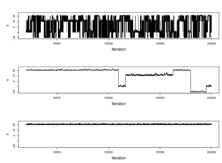
Figure 2: For the algorithms ALPS, LAIS and PT respectively, the trace plots of the first component of the Markov chain in a representative run from each of the 10 repetitions. ALPS (top) successfully explores the 4 modes centred on 20,-10,10 and 20 with rapid inter-modal mixing. In contrast LAIS only manages to make five jumps to another mode whilst the chain in PT remains trapped in the initialisation mode.

The trace plots alone show that ALPS has vastly outperformed LAIS and PT. Figure 3 shows the running estimate of the probability that the first marginal component of the target distribution is less than $1/2$ for each of the 10 repetitions for each of the algoithms. The entity being estimated is $\mathbb{P}(X_{1}<1/2)$, which equals almost exactly 0.5. Therefore, for the $i^{th}$ iteration of the Markov chain with burnin $b$, then the following functional is being plotted for each repetition

$$f(i)=\frac{1}{i-b-1}\sum_{j=b+1}^{i}\mathbbm{1}_{\{x_{1}^{j}<1/2\}}$$ (26)

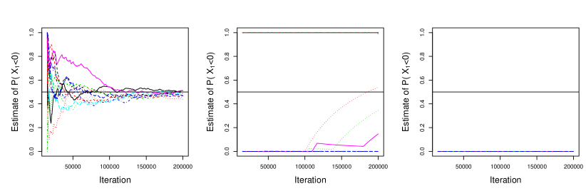
Figure 3: For the algorithms ALPS, LAIS and PT respectively, the function in equation 26 with a burn-in $b=15,000$ is plotted for each of the 10 repetitions. For ALPS (left-most plot) all trajectories concentrate around the truth by the end of their runs, whilst LAIS and PT fail dramatically in estimating this basic quantity.

The plot for the runs of ALPS show that all repetitions converge successfully towards the true value of 0.5 whilst PT and LAIS fail to estimate this probability successfully.

All three algorithms have been run to give the same output quantity at the target state. However, it takes different amounts of time to run each algorithm per iteration. Table 1 shows the average run time for each of the three algorithms across each of the 10 repetitions.

Algorithm	ALPS	LAIS	PT
Run Time (sec)	276.7	57.2	529.6

Table 1: Comparison of the observed average run times for each of the three algorithms.

The results in Table 1 are very complementary to ALPS since there appears to be little extra cost in running ALPS for what has been shown to be a dramatic gain in sample output. Indeed ALPS appears less expensive than PT and this is simply due to the vast number of extra temperatures that PT is updating per step of the chain in this example. However, in this example the number of modes was known and so the mode finding could be optimised for ALPS and LAIS; something not possible in a real data example where one may continue mode searching throughout the duration or even doing some pre-computation dedicated to mode searches (as was the case in the following real data example in Section 6.2).

6.2 Example 2: Seemingly-Unrelated Regression Model

Multiresponse models (Searle and Khuri, 2017, ch. 14) arise from datasets that have more than one dependent variable, where these variables are correlated with each other. An important example is Seemingly-Unrelated Regression (SUR or SURE), which was introduced by Zellner (1962). A wide variety of different SUR models are described by Srivastava and Giles (1987) and the review of Fiebig (2001). These models involve a system of $M$ linear regression equations, one for each response, $m=1,\dots,M$:

$$\vec{y}_{m}=\mathbf{X}_{m}\vec{\theta}_{m}+\vec{\epsilon}_{m},$$ (27)

where $\vec{y}_{m}$ is a column vector of $N_{m}$ observations for the $m$th respnse, $\vec{\theta}_{m}$ is a vector of $J_{m}$ regression coefficients, $\mathbf{X}_{m}$ is an $N_{m}\times J_{m}$ matrix of covariates, and $\vec{\epsilon}_{m}$ is a vector of residual errors. For notational convenience, we assume that $N_{1}=N_{2}=\dots=N_{M}=N$ and likewise that $J_{1}=J_{2}=\dots=J_{M}=J$, although in full generality that is not always the case. For example, (Kmenta, 1986, p. 687) included a SUR model with $J_{1}=2$ and $J_{2}=3$ covariates.

The vectors of observations can be stacked on top of each other to form a single, longer vector $\left(\vec{y}_{1}^{T},\vec{y}_{2}^{T},\dots,\vec{y}_{M}^{T}\right)^{T}$ and similarly with the regression coefficents $\left(\vec{\theta}_{1}^{T},\vec{\theta}_{2}^{T},\dots,\vec{\theta}_{M}^{T}\right)^{T}$. The covariates $\mathbf{X}_{m}$ are combined to form a $MN\times MP$ block-diagonal matrix, resulting in the regression equation:

$$\left[\begin{array}[]{c}\vec{y}_{1}\\ \vec{y}_{2}\\ \vdots\\ \vec{y}_{M}\end{array}\right]=\left[\begin{array}[]{cccc}\mathbf{X}_{1}&&\dots&\mathbf{0}\\ &\mathbf{X}_{2}&&\vdots\\ \vdots&&\ddots&\\ \mathbf{0}&\dots&&\mathbf{X}_{M}\end{array}\right]\left[\begin{array}[]{c}\vec{\theta}_{1}\\ \vec{\theta}_{2}\\ \vdots\\ \vec{\theta}_{M}\end{array}\right]+\left[\begin{array}[]{c}\vec{\epsilon}_{1}\\ \vec{\epsilon}_{2}\\ \vdots\\ \vec{\epsilon}_{M}\end{array}\right].$$ (28)

The errors $\vec{\epsilon}_{m}$ are assumed to be jointly multivariate normal,

$$\bm{\epsilon}\sim\mathcal{N}\left(\vec{0},\,\bm{\Sigma}_{\epsilon}\otimes\mathbf{I}\right),$$

where $\mathbf{I}$ is a $N\times N$ identity matrix and $\bm{\Sigma}_{\epsilon}$ is a $M\times M$ variance-covariance matrix with entries $\sigma^{2}_{\ell,m}$. Zellner (1962) introduced an asymptotically-unbiased estimator for $\bm{\Sigma}_{\epsilon}$, conditional on estimates $\hat{\bm{\theta}}$ of the regression coefficients:

$$\hat{\sigma}^{2}_{\ell,m}=\frac{1}{N}\left(\vec{y}_{\ell}-\mathbf{X}_{\ell}\hat{\theta}_{\ell}\right)^{T}\left(\vec{y}_{m}-\mathbf{X}_{m}\hat{\theta}_{m}\right).$$

Given an estimate of $\widehat{\bm{\Sigma}}_{\epsilon}$, $\hat{\bm{\theta}}$ can be estimated using generalised least squares (Aitken, 1936). Let $\widehat{\bm{\Omega}}=(\widehat{\bm{\Sigma}}_{\epsilon}\otimes\mathbf{I})^{-1}$, then

$$\hat{\bm{\theta}}=\left(\mathbf{X}^{T}\widehat{\bm{\Omega}}\mathbf{X}\right)^{-1}\mathbf{X}^{T}\widehat{\bm{\Omega}}\mathbf{y}.$$

Alternating between these two estimators results in an iterative procedure that converges to a solution to the simultaneous regression equations.

The profile log-likelihood of the SUR model is thus:

$$\ell(\mathbf{Y}\mid\hat{\bm{\theta}})=-N\log\{2\pi\}-\frac{N}{2}\log\left\{\left|\widehat{\bm{\Sigma}}_{\epsilon}\right|\right\}-N$$ (29)

Due to the quadratic form of the SUR model, it was long assumed that its likelihood was log-concave and therefore the iterative estimation procedure of Zellner (1962) was guaranteed to converge to the global maximum. For example, see (Srivastava and Giles, 1987, p. 157) and (Greene, 1997, p. 686). However, in fact these models are an example of a curved exponential family (Sundberg, 2010). Drton and Richardson (2004) showed in the bivariate case that maximising (29) is equivalent to finding the real roots of a fifth-degree polynomial. The profile log-likelihood preserves all stationary points of the log-likelihood, so if the likelihood is multi-modal then so will $\ell(\mathbf{Y}\mid\bm{\theta})$ (Drton and Richardson, 2004, Lemma 1). This means that the likelihood could have one, two, or three local maxima. Drton and Richardson (2004) provided a specific example of a dataset where the SUR model exhibits two local modes, which we will examine in more detail in the following section.

6.2.1 Bimodal Example

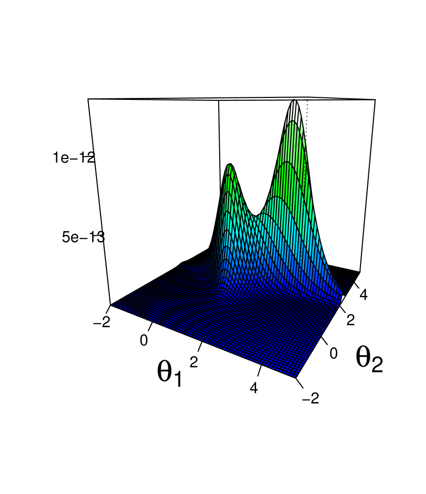
(a) Target distribution

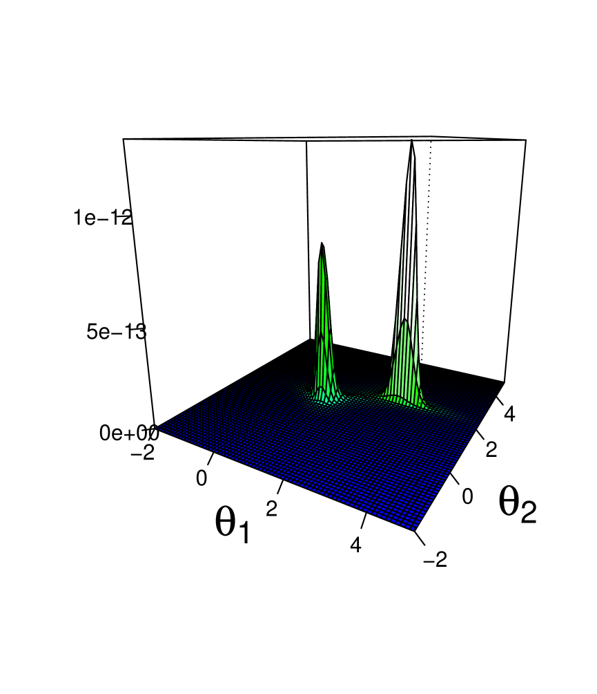
(b) Coldest temperature

Figure 4: (a) 3D perspective plot of the profile likelihood (29) for the bivariate SUR model, adapted from (Drton and Richardson, 2004, Fig. 1); (b) Annealed likelihood at the coldest temperature level used in ALPS.

In the simplest, bivariate case with $M=2$ responses and only $J=1$ covariates per response, the model (28) can be written as:

$$\left[\begin{array}[]{c}\vec{y}_{1}\\ \vec{y}_{2}\end{array}\right]=\left[\begin{array}[]{cc}\vec{x}_{1}&\vec{0}\\ \vec{0}&\vec{x}_{2}\end{array}\right]\left[\begin{array}[]{c}\theta_{1}\\ \theta_{2}\end{array}\right]+\left[\begin{array}[]{c}\vec{\epsilon}_{1}\\ \vec{\epsilon}_{2}\end{array}\right].$$

Drton and Richardson (2004) featured an example dataset with $N=8$ observations. The profile likelihood (29) is illustrated in Figure 4(a). There are two modes at $\bm{\theta}=$ (0.78, 1.54) and (2.76, 2.50) and a saddle point at (1.62, 2.03). The iterative algorithm is initialised at the ordinary least squares estimate, $\hat{\bm{\theta}}=$ (1.25, 1.78). Using the R package ‘systemfit’ (Henningsen and Hamann, 2007) with a tolerance level of $10^{-6}$, the algorithm of Zellner (1962) converges to the first mode after 25 iterations. However, the profile log-likelihood at this mode is -27.72, whereas at the other mode it is -27.35. This algorithm has failed to find the global maximum.

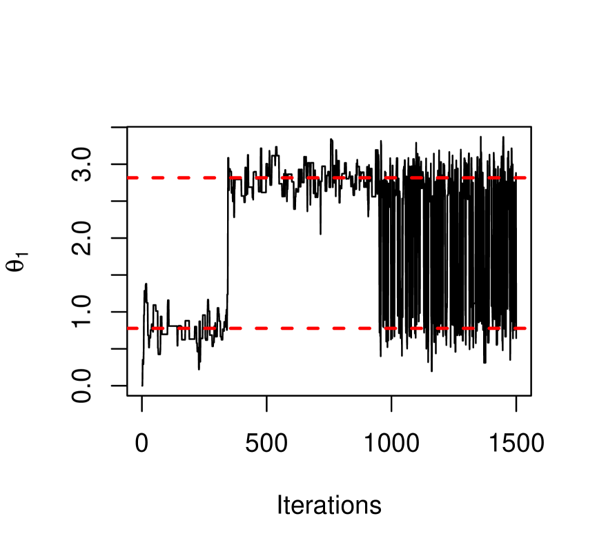
(a) Traceplot for $\theta_{1}$.

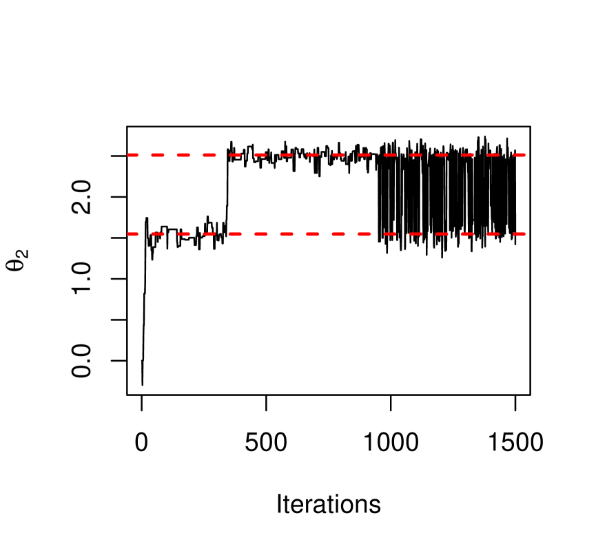
(b) Traceplot for $\theta_{2}$.

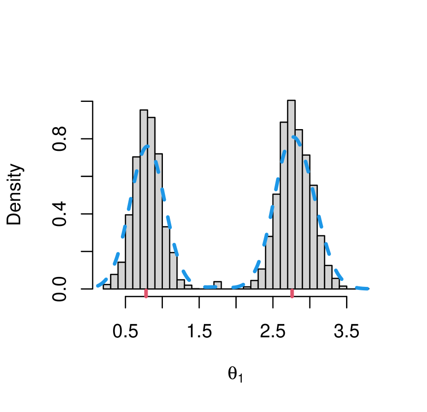
(c) Histogram for $\theta_{1}$.

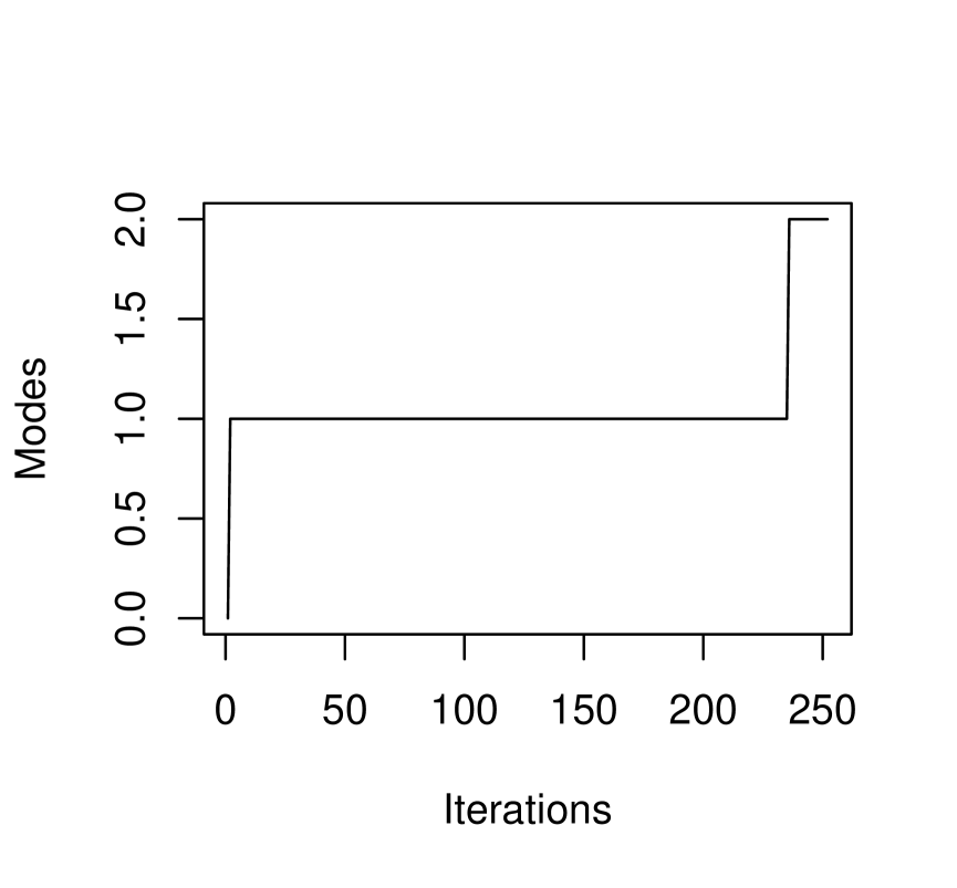
(d) Mode finder.

Figure 5: Results for ALPS with the bivariate SUR model from Drton and Richardson (2004). The red, dashed lines show the locations of the two modes. Note that the ratio between the hot-state mode finder and the other chains is 1:4, so 236 iterations of the mode finder corresponds to 944 iterations of the other chains. Therefore, the first 1,000 iterations should be discarded as burn-in.

We run ALPS using the same profile log-likelihood function, with three inverse temperature levels $(1,\sqrt{10},10)$ as well as the hot state 0.5. The profile likelihood at the coldest temperature level is illustrated in Figure 4(b). The hot-state mode finder locates both modes after 236 iterations, as shown in Figure 5(d), and it takes 2.6 seconds for 10,000 iterations in total. The MCMC trace plots for the two parameters at the coldest temperature are shown in Figures 5(a) and 5(b), respectively, and a histogram for $\theta_{1}$ is shown in Figure 5(c). The jump rate for mode-hopping proposals was 0.9 at the coldest temperature, with acceptance rates of 0.067 for the hot-state mode finder, 0.265 for within-temperature moves and 0.331 for position-dependent moves at the target temperature. The temperature-swapping acceptance rate was 0.508 between the first two temperatures, and 0.847 at the coldest temperature.

6.2.2 Investment Demand

Zellner (1962) illustrated his method using an investment equation with $J=3$ terms,

$$\vec{y}_{m}=\vec{x}_{1,m}\theta_{1,m}+\vec{x}_{2,m}\theta_{2,m}+\vec{x}_{3,m}\theta_{3,m}+\vec{\epsilon}_{m},$$

where $y_{i,m}$ is the gross investment by firm $m$ during the $i$th year, $\vec{x}_{1,m}$ is a vector of ones (so that $\theta_{1,m}$ is a firm-specific intercept), $\vec{x}_{2,m}$ is the market value of the firm, and $\vec{x}_{3,m}$ is its capital stock. The dataset of U.S. manufacturing firms was originally published by Grunfeld (1958) and has since received considerable attention in the econometrics literature, as reviewed by Kleiber and Zeileis (2010). We will consider the first $N=15$ years of data, from 1935 to 1949, for $M=5$ firms (General Motors, Chrysler, General Electric, Westinghouse, and US Steel), so the parameter space has 15 dimensions in total. These data are available in the R package ‘systemfit’ Henningsen and Hamann (2007).

The iterative algorithm of Zellner (1962) takes 52 iterations to converge to a local mode, with a sum of squared residuals (SSR) of 216,943 and profile log-likelihood of -263.7. We run ALPS with seven inverse temperature levels (1.00, 1.10, 1.40, 1.96, 2.74, 3.84, 5.38) and hot state 1/15 = 0.067. Three modes are located as shown in Figure 6(d), although the third mode has negligible probability mass. The first mode discovered by the EC part of ALPS matches the estimate from ‘systemfit,’ while the other two modes have profile log-likelihoods of -264.9 and -329.1, respectively.

There were a number of trial runs undertaken to tune the EC’s inverse temperature. As mentioned in the previous empirical example above, this is the component of the ALPS procedure that is most difficult to tune in a real problem when you don’t know the answer. This example further showed that there will be problem-specific considerations towards making the EC component operate successfully. This has motivated future work into more robust techniques for the EC phase of the algorithm, e.g. using more hot-state temperature levels.

This problem is particularly ill-posed due to parameter unidentifiability (which leads to the multimodality in the posterior). In this problem, despite attempts to reparameterize, there remain issues with the modes of the posterior distribution being located on long, thin ridges that seem to decay with significantly heavier tails than Gaussian. This means that to obtain a good Laplace approximation to the mode the ALPS procedure would need to use very large inverse temperature values. However, when this was attempted it led to severe computational issues with regards to machine precision, likely due to the condition numbers of the Hessians at the mode points, illustrating the ill-posed nature of the problem. To overcome this a truncated version of the annealed HAT targets was utilised for annealed temperatures with $\beta>1$. These are a small modification to the HAT targets and they are defined and discussed in detail in Appendix B.

With the setup described and using the modified truncated HAT targets, it took 31 minutes for 200,000 iterations of ALPS. The MCMC trace plot for the ninth parameter (General Electric capital stock) at the coldest temperature is shown in Figure 6(a). Full results for all 15 parameters at 7 temperature levels are provided in the online supplementary material. The jump rate for mode-hopping proposals was 0.256 at the coldest temperature, with acceptance rates of 0.147 for the EC component random walk Metropolis algorithm, 0.350 for within-temperature moves and 0.380 for position-dependent moves at the target temperature. The temperature-swapping acceptance rates were 0.325 between the first two inverse temperatures and 0.725 at the coldest temperature.

ALPS is not ideally suited to this example. The modes are not especially well-separated and the modes lie on narrow ridges which lead to computational instability. The success of the algorithm to still draw a sample from multiple modes demonstrates the robustness of the approach outside the canonical setting.

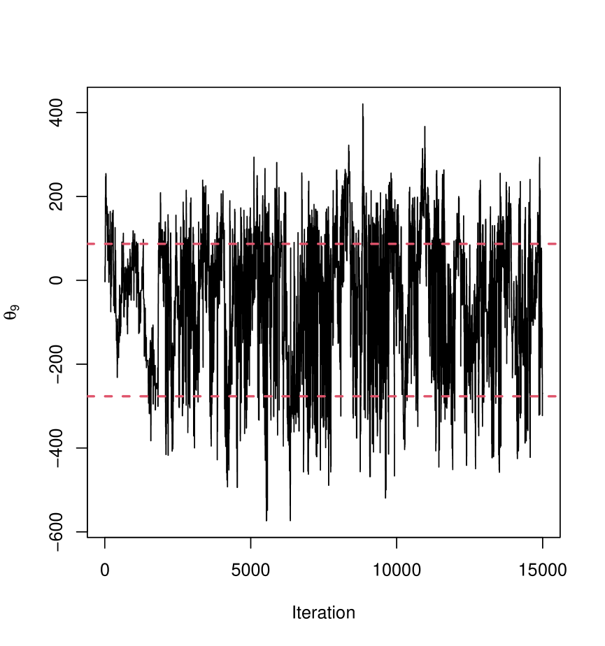
(a) Traceplot for $\theta_{9}$ at the target temperature.

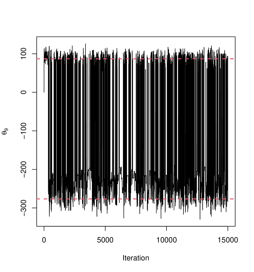
(b) Traceplot for $\theta_{9}$ at the coldest temperature.

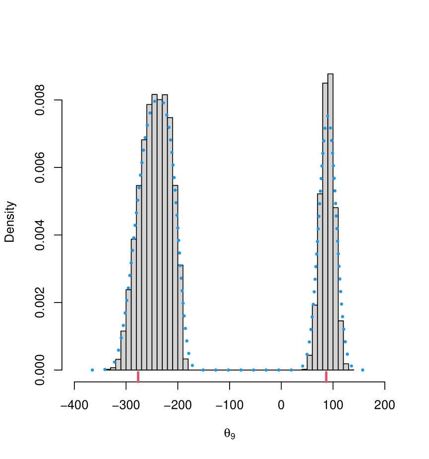
(c) Histogram for $\theta_{9}$.

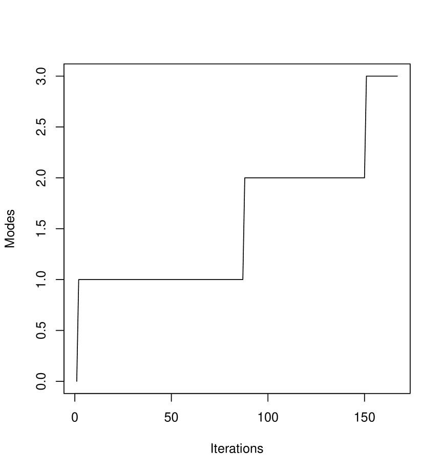
(d) Mode finder.

Figure 6: Results for ALPS with the SUR dataset from Grunfeld (1958) with $N=15$ years of observations for $M=5$ manufacturing firms, with $J=3$ covariates per firm. The red, dashed lines show the locations of two of the modes (the third mode has negligible probability mass).

7 Conclusion and Further Work

This paper introduces a novel algorithm, ALPS, that is designed to sample effectively and scalably from multimodal distributions that have support on $\mathbb{R}^{d}$ and are $C^{2}$. The main methodological contribution of this paper is that this problem can be solved by (localised) annealing rather than tempering and that this new approach mitigates many of the issues due to mode heterogeneity that plague traditional methods for these problems. Also, ALPS exploits recent advancements in the PT literature that both enable the algorithm to be stable in high-dimensions as well as providing substantially accelerated performance.

The accompanying theoretical contribution of the paper shows that the coldest temperature required for the procedure will be $\mathcal{O}(d)$ under suitable regularity conditions. This gives both guidance on tuning the algorithm and demonstrates polynomial computational complexity cost of $\mathcal{O}(d^{3})$.

There are a number of further considerations regarding adding robustness and practicality to the ALPS procedure. Many of the ideas for exploration are already alluded to in the paper: improving the effectiveness of the EC part by running more than one exploration chain and having multiple temperature levels; parallel implementation of the PA and EC parts of ALPS; and introducing weightings to regions to stabilise the inter-modal masses when the HAT targets don’t sufficiently preserve the weights. Adapting the ideas of ALPS to facilitate an automatic and scalable reversible jump MCMC algorithm is the immediate focus for further work.

Appendix A Proofs

The proof of Theorem 4.1 relies on Lemmata 4.2, 4.3 and 4.4. The proofs of these were deferred to this section. There are a number of preliminary results that are essential in the main proofs.

For notational convenience herein denote

$$B_{\epsilon}(L):=\{x\in\mathbb{R}:|x-L|<\epsilon\}$$

and formally define the normalisation constant.

Definition A.1 (Normalisation at level $\beta$).

For the un-normalised marginal component of the product target specified in Theorem 4.1, i.e. $f(\cdot)$, then define the normalisation constant

$$N(\beta):=\int[f(x)]^{\beta}dx$$ (30)

Definition A.2 (Asymptotic Gaussian standard deviation).

With $f(\cdot)$ as in Theorem 4.1 with $H=h^{\prime\prime}(0)$, define

$$\sigma(\beta)=\frac{1}{\sqrt{\beta|H|}}.$$ (31)

The following few propositions work on integrals that use the un-normalised density. It will be clear when the normalisation constant comes in. In fact, it will be shown that $N(\beta)=\mathcal{O}(\beta^{1/2})$.

Proposition 3 (Exponential decay of tail integrals).

With $f(\cdot)$ as in Theorem 4.1 and specifically for the polynomial tail condition given in (16) then for each $k\geq 0$ there exists constants $C_{1}>0\leavevmode\nobreak\ \text{and}\leavevmode\nobreak\ C_{2}\geq 0$ such that

$$\limsup_{\beta\rightarrow\infty}\left|e^{C_{1}\beta}\int_{\mathbb{R}\backslash B_{M}(0)}z^{k}f^{\beta}(z)dz\right|=C_{2}<\infty$$

Proof.

With $K,\gamma\leavevmode\nobreak\ \text{and}\leavevmode\nobreak\ M$ all specified in (16) (and wlog $K<M$) and assuming $\beta$ sufficiently large

$$\left|\int_{M}^{\infty}z^{k}f^{\beta}(z)dz\right| \leq \int_{M}^{\infty}|z|^{k}|z|^{-\gamma\beta}\frac{f^{\beta}(z)}{|z|^{-\gamma\beta}}dz$$

$$\leq K^{\beta}\int_{M}^{\infty}|z|^{k-\gamma\beta}dz$$

$$\leq \frac{K}{M}^{\beta}\frac{M^{4}}{\left(\gamma\beta-(k+1)\right)}$$

$$= \frac{M^{4}}{\left(\gamma\beta-(k+1)\right)}e^{-\beta|\log(K/M)|}$$

and thus the conclusion of the proposition follows trivially. ∎

Herein, for notational convenience, we denote

$$I_{k}(a,b):=\int_{a}^{b}z^{k}f^{\beta}(z)dz$$

Proposition 4 (Intermediate integral exponential decay).

For $r\leq 1/3$ and $f(\cdot)$ as in Theorem 4.1, specifically the Dutchman’s cap assumption in (17), then for each $k\geq 0$ there exists constants $D_{1}>0$ such that

$$\limsup_{\beta\rightarrow\infty}\left|e^{D_{1}\beta^{(1-2r)}}\left(I_{k}(-M,-M\beta^{-r})+I_{k}(M\beta^{-r},M)\right)\right|=0<\infty$$ (32)

Proof.

Take $\delta_{2}$ as specified in the Dutchman’s cap assumption in (17) and recall we have

$$f(z)\leq\begin{cases}\exp\left(-z^{2}\frac{|H|}{4}\right),&\text{if $|z|<\delta_{2}$}.\\ \exp\left(-\delta_{2}^{2}\frac{|H|}{4}\right),&\text{if $\delta_{2}\leq|z|\leq M$}.\end{cases}$$ (33)

Assume that $\beta$ is sufficiently large so that $M\beta^{-r}<\delta_{2}$. By splitting the integral

$$I_{k}(M\beta^{-r},M)=I_{k}(M\beta^{-r},\delta_{2})+I_{k}(\delta_{2},M).$$

Focusing on the first term and using (32) and noting that $1-2r>0$

$$|I_{k}(M\beta^{-r},\delta_{2})| = \int_{M\beta^{-r}}^{\delta_{2}}z^{k}f^{\beta}(z)dz\leq\int_{M\beta^{-r}}^{\delta_{2}}z^{k}\exp\left(-z^{2}\beta\frac{|H|}{4}\right)dz$$ (34)

$$\leq \int_{M\beta^{-r}}^{\delta_{2}}\delta_{2}^{k}\exp\left(-M^{2}\beta^{(1-2r)}\frac{|H|}{4}\right)dz$$

$$= \delta_{2}^{k}\left[\delta_{2}-M\beta^{-r}\right]\exp\left(-M^{2}\beta^{(1-2r)}\frac{|H|}{4}\right).$$

Then for the second term again using (32) then

$$|I_{k}(\delta_{2},M)| = \int_{\delta_{2}}^{M}z^{k}\frac{f^{\beta}(z)}{N(\beta)}dz\leq\frac{\sqrt{\beta}}{J}\int_{\delta_{2}}^{M}M^{k}\exp\left(-\delta_{2}^{2}\beta\frac{|H|}{4}\right)dz$$ (35)

$$\leq (M-\delta_{2})M^{k}\exp\left(-\delta_{2}^{2}\beta\frac{|H|}{4}\right).$$

Combining (34), (35) and an identical procedural application to the lower integrand, $I_{k}(-M,-M\beta^{-r})$, then the proposition is proven. ∎

Lemma A.3 (Limiting integrals).

For $f(\cdot)$ in Theorem 4.1

$$\lim_{\beta\rightarrow\infty}\left\{\beta^{g(k)}\sqrt{\frac{\beta|H|}{2\pi}}\int_{\mathbb{R}}z^{k}f^{\beta}(z)dz\right\}=\begin{cases}\frac{\mathbb{E}(S^{k+3})h^{\prime\prime\prime}(0)}{6|H|^{(k+3)/2}},&\text{if $k$ is odd}.\\ \frac{\mathbb{E}(S^{k})}{|H|^{k/2}},&\text{if $k$ is even}\end{cases}$$ (36)

where $S$ is distributed according to a standard normal distribution, i.e. $N(0,1)$, and

$$g(k)=\begin{cases}\frac{k+3}{2}-2,&\text{if $k$ is odd}\\ \frac{k}{2},&\text{if $k$ is even}.\end{cases}$$

Proof.

By Propositions 3 and 4 then one can derive that for $r=1/3$

$$I_{k}(-\infty,\infty)=I_{k}(-M\beta^{-r},M\beta^{-r})+R(\beta)$$ (37)

where $R(\beta)=\mathcal{O}\left(\exp\left(-D\beta^{(1-2r)}\right)\right)$ for some constant $D>0$ i.e. exponentially decaying in $\beta$. Consequently, we focus on $I_{k}(-M\beta^{-r},M\beta^{-r})$.

By Taylor expansion with Taylor remainder $|\xi_{z}|<|z|$

$$f^{\beta}(z) = \exp\left(\beta\left[z^{2}\frac{H}{2}+z^{3}\frac{h^{\prime\prime\prime}(0)}{6}+z^{4}\frac{h^{\prime\prime\prime\prime}(\xi_{z})}{24}\right]\right)$$ (38)

$$= \sqrt{\frac{2\pi}{\beta|H|}}\phi_{\beta}(z)\exp\left(\beta z^{3}\frac{h^{\prime\prime\prime}(0)}{6}\right)\exp\left(\beta z^{4}\frac{h^{\prime\prime\prime\prime}(\xi_{z})}{24}\right)$$

where $\phi_{\beta}(\cdot)$ denotes the pdf of a $N(0,\sigma(\beta)^{2})$.

By further Taylor expansion

$$\exp\left(\beta z^{3}\frac{h^{\prime\prime\prime}(0)}{6}\right) = 1+\beta z^{3}\frac{h^{\prime\prime\prime}(0)}{6}+\beta^{2}z^{6}\frac{h^{\prime\prime\prime}(0)^{2}}{72}e^{\xi^{1}_{(\beta,z)}}$$ (39)

$$\exp\left(\beta z^{4}\frac{h^{\prime\prime\prime\prime}(\xi_{z})}{24}\right) = 1+\beta z^{4}\frac{h^{\prime\prime\prime\prime}(\xi_{z})}{24}e^{\xi^{2}_{(\beta,z)}}$$ (40)

where $\xi^{1}_{(\beta,z)}$ and $\xi^{2}_{(\beta,z)}$ are Taylor remainders such that

$$|\xi^{1}_{(\beta,z)}| \leq \left|\beta z^{3}\frac{h^{\prime\prime\prime}(0)}{6}\right|$$ (41)

$$|\xi^{2}_{(\beta,z)}| \leq \left|\beta z^{4}\frac{h^{\prime\prime\prime\prime}(\xi_{z})}{24}\right|.$$ (42)

Combining (38), (39) and (40)

$$I_{k}(-M\beta^{-r},M\beta^{-r})=\sqrt{\frac{2\pi}{-\beta H}}\sum_{m=1}^{6}T_{m}(k)$$ (43)

where

$$T_{1}(k) = \int_{-M\beta^{-r}}^{M\beta^{-r}}z^{k}\phi_{\beta}(z)dz$$

$$T_{2}(k) = \int_{-M\beta^{-r}}^{M\beta^{-r}}\beta z^{k+3}\frac{h^{\prime\prime\prime}(0)}{6}\phi_{\beta}(z)dz$$

$$T_{3}(k) = \int_{-M\beta^{-r}}^{M\beta^{-r}}\beta^{2}z^{k+6}\left(\frac{h^{\prime\prime\prime}(0)^{2}}{72}\right)e^{\xi^{1}_{(\beta,z)}}\phi_{\beta}(z)dz$$

$$T_{4}(k) = \int_{-M\beta^{-r}}^{M\beta^{-r}}\beta z^{k+4}\left(\frac{h^{\prime\prime\prime\prime}(\xi_{z})}{24}\right)e^{\xi^{2}_{(\beta,z)}}\phi_{\beta}(z)dz$$

$$T_{5}(k) = \int_{-M\beta^{-r}}^{M\beta^{-r}}\beta^{2}z^{k+7}\left(\frac{h^{\prime\prime\prime}(0)}{6}\right)\left(\frac{h^{\prime\prime\prime\prime}(\xi_{z})}{24}\right)e^{\xi^{2}_{(\beta,z)}}\phi_{\beta}(z)dz$$

$$T_{6}(k) = \int_{-M\beta^{-r}}^{M\beta^{-r}}\beta^{3}z^{k+10}\left(\frac{h^{\prime\prime\prime}(0)^{2}}{72}\right)\left(\frac{h^{\prime\prime\prime\prime}(\xi_{z})}{24}\right)e^{\xi^{1}_{(\beta,z)}}e^{\xi^{2}_{(\beta,z)}}\phi_{\beta}(z)dz.$$

Consider the case that $k=3$ and all others follow by identical methodology. For $k=3$ it is clear that $T_{1}(3)=0$ so consider $T_{3}(3)$ with (41) and using the fact that $e^{x}\leq e^{|x|}$ and $r=1/3$

$$|T_{3}(3)| \leq \int_{-M\beta^{-r}}^{M\beta^{-r}}\beta^{2}|z|^{9}\left(\frac{h^{\prime\prime\prime}(0)^{2}}{72}\right)\exp\left[\beta|z|^{3}\left|\frac{h^{\prime\prime\prime}(0)}{6}\right|\right]\phi_{\beta}(z)dz$$ (44)

$$\leq \beta^{2}\left(\frac{h^{\prime\prime\prime}(0)^{2}}{72}\right)\exp\left[M^{3}\left|\frac{h^{\prime\prime\prime}(0)}{6}\right|\right]\int_{-M\beta^{-r}}^{M\beta^{-r}}|z|^{9}\phi_{\beta}(z)dz$$

$$\leq \beta^{2}\left(\frac{h^{\prime\prime\prime}(0)^{2}}{72}\right)\exp\left[M^{3}\left|\frac{h^{\prime\prime\prime}(0)}{6}\right|\right]\int_{\mathbb{R}}|z|^{9}\phi_{\beta}(z)dz$$

$$= C_{3}^{3}\beta^{2}\int_{\mathbb{R}}|z|^{9}\phi_{\beta}(z)dz$$

where $C^{3}_{3}\in\mathbb{R}_{+}$ is a constant.

Similarly, there exists constants $C_{4}^{3},C_{5}^{3},C_{6}^{3}$ such that

$$|T_{4}(3)| \leq C_{4}^{3}\beta\int_{\mathbb{R}}|z|^{7}\phi_{\beta}(z)dz$$ (45)

$$|T_{5}(3)| \leq C_{5}^{3}\beta^{2}\int_{\mathbb{R}}|z|^{10}\phi_{\beta}(z)dz$$ (46)

$$|T_{6}(3)| \leq C_{6}^{3}\beta^{3}\int_{\mathbb{R}}|z|^{13}\phi_{\beta}(z)dz.$$ (47)

Routine calculations using integration by parts reveals that

$$\int_{\mathbb{R}}|z|^{m}\phi_{\beta}(z)dz\leq\begin{cases}\frac{96}{\sqrt{2\pi}(\beta|H|)^{7/2}},&\text{if $m=7$}\\ \frac{1536}{\sqrt{2\pi}(\beta|H|)^{9/2}},&\text{if $m=9$}\\ \frac{945}{(\beta|H|)^{5}},&\text{if $m=10$}\\ \frac{92160}{\sqrt{2\pi}(\beta|H|)^{13/2}},&\text{if $m=13$}\\ \end{cases}$$ (48)

Combining (44), (45), (46), (47) and (48) shows that for $m\in\{3,4,5,6\}$

$$|T_{m}(3)|\leq\mathcal{O}\left(\frac{1}{\beta^{5/2}}\right).$$ (49)

Hence the crucial term is $T_{2}(3)$,

$$T_{2}(3) = \int_{-M\beta^{-r}}^{M\beta^{-r}}\beta z^{6}\frac{h^{\prime\prime\prime}(0)}{6}\phi_{\beta}(z)dz$$

$$= \frac{h^{\prime\prime\prime}(0)}{6}\beta\int_{\mathbb{R}}z^{6}\phi_{\beta}(z)dz+R_{2}(3)$$

where using identical methodology to Propositions 3 and 4 one can show that for a constant $F>0$ then $R_{2}(3)=\mathcal{O}\left(\beta^{5/2}e^{-F\beta^{2/3}}\right)$ and so trivially $R_{2}(3)=\mathcal{O}\left(\beta^{-5/2}\right)$. Hence,

$$T_{2}(3)=\frac{15h^{\prime\prime\prime}(0)}{6\beta^{2}|H|^{3}}+\mathcal{O}\left(\beta^{-5/2}\right).$$ (50)

Thus combining the results of (37), (43), (49) and (51) then

$$\lim_{\beta\rightarrow\infty}\left\{\beta^{2}\sqrt{\frac{\beta|H|}{2\pi}}\int_{\mathbb{R}}z^{k}f^{\beta}(z)dz\right\}=\frac{15h^{\prime\prime\prime}(0)}{6|H|^{3}}.$$ (51)

This proves the lemma for k=3 and identical methodology all other values of $k\in\mathbb{N}_{0}$ follow. ∎

For the purposes of proving the main result the following corollary concatenates the key results from Lemma A.3.

Corollary 1 (Key moment results).

From Lemma A.3 and the details of the proof it can be concluded that:

$$N(\beta) = \sqrt{\frac{2\pi}{-\beta H}}+\mathcal{O}\left(\beta^{-1}\right)$$ (52)

$$\mu_{\beta}:=\int_{\mathbb{R}}z^{3}\frac{f^{\beta}(z)}{N(\beta)}dz = \frac{15h^{\prime\prime\prime}(0)}{6\beta^{2}|H|^{3}}+\mathcal{O}\left(\beta^{-5/2}\right)$$ (53)

$$\sigma^{2}_{\beta}:=\int_{\mathbb{R}}z^{6}\frac{f^{\beta}(z)}{N(\beta)}dz = \frac{15}{\beta^{3}|H|^{3}}+\mathcal{O}\left(\beta^{-7/2}\right)$$ (54)

Proof.

All methodology and details from Lemma A.3 above. ∎

Now with the results established in Corollary 1 we are in a position to prove the core lemmata that establish the result of Theorem 4.1.

Proof of Lemma 4.2.

Recalling that in the setup of Theorem 4.1 we have $\beta=\ell d$. We aim to show that as $d\rightarrow\infty$

$$W(d):=\sum_{i=1}^{d}\frac{\beta h^{\prime\prime\prime}(0)}{6}(y_{i}^{3}-x_{i}^{3})\Rightarrow N\left(-\frac{15h^{\prime\prime\prime}(0)^{2}}{36\ell|H|^{3}},\frac{30h^{\prime\prime\prime}(0)^{2}}{36\ell|H|^{3}}\right).$$

Since the distribution of the $x_{i}$ and $y_{i}$ is dependent on $d$ then we are in the situation of triangular arrays. As such we aim to use the Lindeberg-Feller theorem, see e.g. Durrett (2010). Define for each $d\in\mathbb{N}$ and for $i\in\{1,\ldots,d\}$

$$X_{(d,i)}:=\left(\frac{\beta h^{\prime\prime\prime}(0)}{6}\right)\left(x_{i}^{3}-\mu_{\beta}\right).$$

Lindeberg-Feller Conditions: To apply the result of the Lindeberg-Feller theorem from Durrett (2010) to the $X_{(d,i)}$’s, it is sufficient to establish the following two conditions as $d\rightarrow\infty$

1. There exists $\sigma^{2}\in\mathbb{R}_{+}$ such that

   $$\sum_{i=1}^{d}\mathbb{E}(X_{(d,i)}^{2})\rightarrow\sigma^{2}>0$$ (55)

2. For all $\epsilon>0$ and with $A_{\epsilon}^{d}:=\{|X_{(d,i)}|>\epsilon\}$

   $$\lim_{d\rightarrow\infty}\sum_{i=1}^{d}\mathbb{E}(|X_{(d,i)}|^{2}\mathbbm{1}_{A_{\epsilon}})=0$$ (56)

It is simple to show that L-F condition (i) in (55) holds, since by (53) and (54)

$$\mathbb{E}\left(X_{(d,i)}^{2}\right)=\frac{30h^{\prime\prime\prime}(0)^{2}}{36\ell d|H|^{3}}+\mathcal{O}\left(d^{-3/2}\right)$$

and so it is immediate that

$$\sum_{i=1}^{d}\mathbb{E}(X_{(d,i)}^{2})\rightarrow\frac{30h^{\prime\prime\prime}(0)^{2}}{36\ell d|H|^{3}}>0$$ (57)

To show that L-F condition (ii) in (56) holds is more involved. To this end let $\epsilon>0$

$$\mathbb{E}(|X_{(d,i)}|^{2}\mathbbm{1}_{A_{\epsilon}^{d}})$$ (58)

$$= \left(\frac{\beta h^{\prime\prime\prime}(0)}{6}\right)^{2}\left[\mathbb{E}\left(x_{i}^{6}\mathbbm{1}_{A_{\epsilon}^{d}}\right)-2\mu_{\beta}\mathbb{E}\left(x_{i}^{3}\mathbbm{1}_{A_{\epsilon}^{d}}\right)+\mu_{\beta}^{2}\mathbb{P}(A_{\epsilon}^{d})\right]$$

$$\leq \left|\frac{\beta h^{\prime\prime\prime}(0)}{6}\right|^{2}\left[\mathbb{E}\left(x_{i}^{6}\mathbbm{1}_{A_{\epsilon}^{d}}\right)-2|\mu_{\beta}|\mathbb{E}\left(|x_{i}|^{3}\mathbbm{1}_{A_{\epsilon}^{d}}\right)+\mu_{\beta}^{2}\mathbb{P}(A_{\epsilon}^{d})\right]$$ (59)

Using identical methodology to that used in proving Lemma A.3 with only a trivial extension one can show that

$$\mathbb{E}\left(|x_{i}|^{3}\mathbbm{1}_{A_{\epsilon}^{d}}\right)\leq\mathcal{O}\left(d^{-3/2}\right)$$

and so with $\mu_{\beta}=\mathcal{O}\left(d^{-2}\right)$ given in (53) then

$$|\mu_{\beta}|\mathbb{E}\left(|x_{i}|^{3}\mathbbm{1}_{A_{\epsilon}^{d}}\right) \leq \mathcal{O}\left(d^{-7/2}\right)$$

$$|\mu_{\beta}^{2}\mathbb{P}(A_{\epsilon}^{d})| \leq |\mu_{\beta}^{2}|=\mathcal{O}\left(d^{-4}\right)$$

and thus we can conclude that

$$\lim_{d\rightarrow\infty}\sum_{i=1}^{d}\left|\frac{\beta h^{\prime\prime\prime}(0)}{6}\right|^{2}\left[2\mu_{\beta}\mathbb{E}\left(x_{i}^{3}\mathbbm{1}_{A_{\epsilon}^{d}}\right)+\mu_{\beta}^{2}\mathbb{P}(A_{\epsilon}^{d})\right]=0.$$ (60)

Consequently we must analyse the behaviour of $\mathbb{E}\left(x^{6}\mathbbm{1}_{A_{\epsilon}^{d}}\right)$. We begin by noting that $A_{\epsilon}^{d}$ can be equivalently written as

$$A_{\epsilon}^{d} = \left\{x>\left(\mu_{\beta}+\frac{6\epsilon}{\beta|h^{\prime\prime\prime}(0)|}\right)^{1/3}\right\}\cup\left\{x<\left(\mu_{\beta}-\frac{6\epsilon}{\beta|h^{\prime\prime\prime}(0)|}\right)^{1/3}\right\}$$ (61)

$$:= F_{+\epsilon}^{d}\cup F_{-\epsilon}^{d}.$$

With this notation,

$$\mathbb{E}\left(x^{6}\mathbbm{1}_{A_{\epsilon}^{d}}\right)=\mathbb{E}\left(x^{6}\mathbbm{1}_{F_{+\epsilon}^{d}}\right)+\mathbb{E}\left(x^{6}\mathbbm{1}_{F_{-\epsilon}^{d}}\right).$$ (62)

By (53) we have that $\mu_{\beta}=\mathcal{O}(d^{-2})$ and so from the equivalent formulation of $A_{\epsilon}^{d}$ in (61) and for $d$ sufficiently large there exists a constant $J>0$ such that

$$F_{+\epsilon}^{d} = \left\{x>\left(\mu_{\beta}+\frac{6\epsilon}{\beta|h^{\prime\prime\prime}(0)|}\right)^{1/3}\right\}$$ (63)

$$\supseteq \left\{x>\frac{J}{d^{1/3}}\right\}.$$

Focusing on the first term on the RHS of (62) and with $M$ from (16)

$$\mathbb{E}\left(x^{6}\mathbbm{1}_{F_{+\epsilon}^{d}}\right)\leq N(\beta)\left[I_{6}(Jd^{-1/3},M)+I_{6}(M,\infty)\right].$$ (64)

By Propositions 3 and 4 then there exists a constant $W_{1}>0$ such that the RHS of (64) is $\mathcal{O}\left(e^{-W_{1}d^{1/3}}\right)$. By identical methodology one can show that there exists $W_{2}>0$ such that

$$\mathbb{E}\left(x^{6}\mathbbm{1}_{F_{-\epsilon}^{d}}\right)\leq\mathcal{O}\left(e^{-W_{2}d^{1/3}}\right)$$

and so with $W_{3}:=\max\{W_{1},W_{2}\}$ then

$$\mathbb{E}\left(x^{6}\mathbbm{1}_{A_{\epsilon}^{d}}\right)=\mathcal{O}\left(e^{-W_{3}d^{1/3}}\right).$$ (65)

Consequently by (65) then

$$\lim_{d\rightarrow\infty}\sum_{i=1}^{d}\left|\frac{\beta h^{\prime\prime\prime}(0)}{6}\right|^{2}\mathbb{E}\left(x_{i}^{6}\mathbbm{1}_{A_{\epsilon}^{d}}\right)=0.$$ (66)

So combining (60) and (66) proves that the second Lindeberg-Feller condition in (56) holds.

With (55) and (56) holding for the triangular array of $X_{(d,i)}$’s then the Lindeberg-Feller theorem implies that that as $d\rightarrow\infty$

$$-\sum_{i=1}^{d}X_{(d,i)}\Rightarrow N\left(0,\frac{15h^{\prime\prime\prime}(0)^{2}}{36\ell|H|^{3}}\right).$$

However, by using the result of (53) that gives an explicit value to the $\mu_{\beta}$ and the definition of the $X_{(d,i)}$’s then

$$-\sum_{i=1}^{d}\frac{\beta h^{\prime\prime\prime}(0)}{6}x_{i}^{3}\Rightarrow N\left(-\frac{15h^{\prime\prime\prime}(0)^{2}}{36\ell|H|^{3}},\frac{15h^{\prime\prime\prime}(0)^{2}}{36\ell|H|^{3}}\right).$$ (67)

For a given $d$, the $y_{i}\sim N(0,(\beta|H|)^{-1})$, thus they too fall in to a triangular arrays setup with

$$\mathbb{E}(y_{i}^{3}) = 0$$ (68)

$$\text{Var}(y_{i}^{3}) = \mathbb{E}(y_{i}^{6})=\frac{15}{\beta^{3}|H|^{3}}$$ (69)

and so setting

$$Y_{(d,i)}=\left(\frac{\beta h^{\prime\prime\prime}(0)}{6}\right)y_{i}^{3}$$

one can follow a simplified version of the above Lindeberg-Feller procedure for the $X_{(d,i)}$’s to establish that as $d\rightarrow\infty$

$$\sum_{i=1}^{d}\frac{\beta h^{\prime\prime\prime}(0)}{6}y_{i}^{3}\Rightarrow N\left(0,\frac{15h^{\prime\prime\prime}(0)^{2}}{36\ell(-h^{\prime\prime}(0))^{3}}\right)$$ (70)

Using the fact that the $x_{i}$’s and $y_{i}$’s are independent along with the weak convergences established in (67) and (70) the result of Lemma 4.2 is established. ∎

Proof of Lemma 4.3.

Recalling the statement of Lemma 4.3, the aim is to show that as $d\rightarrow\infty$

$$T_{1}(d):=\sum_{i=1}^{d}\frac{\beta h^{\prime\prime\prime\prime}(0)}{24}\left(y_{i}^{4}-x_{i}^{4}\right)\rightarrow 0\leavevmode\nobreak\ \leavevmode\nobreak\ \text{in}\leavevmode\nobreak\ \leavevmode\nobreak\ \mathbb{P}.$$

To this end fix $\epsilon>0$. Using identical methodology to that used in Lemma A.3 then it can be shown that

$$\mathbb{E}(x_{i}^{4}) = \frac{3}{\left(\beta|H|\right)^{2}}+\mathcal{O}\left(\beta^{-3}\right)$$ (71)

$$\mathbb{E}(x_{i}^{8}) = \frac{105}{\left(\beta|H|\right)^{4}}+\mathcal{O}\left(\beta^{-5}\right)$$ (72)

and from standard calculations using the Gaussianity of the $y_{i}$’s

$$\mathbb{E}(y_{i}^{4}) = \frac{3}{\left(\beta|H|\right)^{2}}$$ (73)

$$\mathbb{E}(y_{i}^{8}) = \frac{105}{\left(\beta|H|\right)^{4}}.$$ (74)

Defining $\mu_{T_{1}(d)}:=\mathbb{E}(T_{1}(d))$ then by (71) and (73) as $d\rightarrow\infty$

$$\mu_{T_{1}(d)}\rightarrow 0.$$ (75)

Thus there exists $U>0$ such that for all $d>U$ then $|\mu_{T_{1}(d)}|<\frac{\epsilon}{2}$. Furthermore, by (71), (73), (72) and (74) then

$$\text{Var}(T_{1}(d))\rightarrow 0\leavevmode\nobreak\ \leavevmode\nobreak\ \text{as}\leavevmode\nobreak\ \leavevmode\nobreak\ d\rightarrow 0.$$ (76)

For $d>U$ and using Chebyshev’s inequality and utilising (76)

$$\mathbb{P}\left(|T_{1}(d)|>\epsilon\right)\leq\mathbb{P}\left(|T_{1}(d)-\mu_{T_{1}(d)}|\geq\frac{\epsilon}{2}\right)\leq\frac{4\text{Var}(T_{1}(d))}{\epsilon^{2}}\rightarrow 0\leavevmode\nobreak\ \leavevmode\nobreak\ \text{as}\leavevmode\nobreak\ \leavevmode\nobreak\ d\rightarrow 0$$

and so the result of Lemma 4.3 holds. ∎

Proof of Lemma 4.4.

Recalling the statement of Lemma 4.4, the aim is to show that as $d\rightarrow\infty$

$$T_{2}(d):=\sum_{i=1}^{d}\frac{\beta}{120}\left(y_{i}^{5}h^{v}(\xi_{y_{i}})-x_{i}^{5}h^{v}(\xi_{x_{i}})\right)\rightarrow 0\leavevmode\nobreak\ \leavevmode\nobreak\ \text{in}\leavevmode\nobreak\ \leavevmode\nobreak\ \mathbb{P}.$$ (77)

To this end, using the assumption given in (15)

$$|T_{2}(d)|\leq\sum_{i=1}^{d}L\frac{\beta}{120}\left(|y_{i}|^{5}+|x_{i}|^{5}\right)=:T_{2}^{r}(d)>0$$ (78)

and so if one can show that $T_{2}^{r}(d)\rightarrow 0$ in $\mathbb{P}$ then the required result in (77) follows. Note that

$$\mathbb{E}(|y_{i}|^{5})=\frac{16}{\sqrt{2\pi}\left(\beta|H|^{5/2}\right)}$$ (79)

and using identical methodology to the proof of Lemma A.3 then it can be shown that for some constant $E\in\mathbb{R}$

$$\mathbb{E}(|x_{i}|^{5})=\frac{E}{d^{5/2}}+\mathcal{O}\left(d^{-3}\right)$$ (80)

Let $\epsilon>0$, then by Markov inequality and then using (79) and (80)

$$\mathbb{P}(T_{r}(d)>\epsilon) \leq \frac{L\ell d}{24\epsilon}\sum_{i=1}^{d}\left[\mathbb{E}(|y_{i}|^{5})+\mathbb{E}(|x_{i}|^{5})\right]$$

$$= \frac{L\ell d^{2}}{24\epsilon}\left[\mathbb{E}(|y_{1}|^{5})+\mathbb{E}(|x_{1}|^{5})\right]$$

$$\rightarrow 0\leavevmode\nobreak\ \leavevmode\nobreak\ \leavevmode\nobreak\ \text{as}\leavevmode\nobreak\ \leavevmode\nobreak\ \leavevmode\nobreak\ d\rightarrow\infty.$$

Thus the result in (77) follows. ∎

Appendix B Truncating the HAT distributions

In Section 6.2.2 the ALPS procedure was used to sample from a posterior distribution that resulted from an SUR model. The condition number of the Hessian evaluations showed that the problem was unstable. The issue is that the problem is ill-posed in that the parameters are essentially unidentifiable. The posterior distribution seems to exhibit narrow ridges with tail-structures in those directions appearing to be significantly heavier than Gaussian.

As such there would need to be significant localised annealing before the target distribution along the ridge directions began to appear sufficiently Gaussian so that the independence sampler could provide reasonable inter-modal jump rates. However, this led to issues with machine precision. To overcome this issue, an ad-hoc adjustment to the HAT targets was proposed. The idea was to introduce a truncated version of the annealed HAT targets that would be exactly as described in Definition 3.3 if the location was within a prescribed distance from the mode point and would be set to zero outside of that. The idea being to eliminate some of the instability of the heavy tailed ridge directions at the annealed temperature levels so that the algorithm works without using annealed temperature levels that would create computational problems due to machine precision issues.

Definition B.1 (Truncated HAT distributions at quantile $q$).

Consider the definition of the HAT distribution at inverse temperature level $\beta$ from Definition 3.3. Then using the same notation as Definition 3.3, and letting $A=A_{(}x,\beta)$ for ease of notation, set

$$Q_{(x,\beta)}:=\mathbbm{1}_{\{(x-\mu_{A})^{T}\Sigma_{A}^{-1}(x-\mu_{A})<q\}}$$ (81)

The truncated HAT distribution at inverse temperature level $\beta$ and quantile $q$ is then defined as:

$$\pi_{\beta}(x)\propto\begin{cases}\pi(x)^{\beta}\pi(\mu_{A_{(x,\beta)}})^{1-\beta}Q_{(x,\beta)}&\text{if $A_{(x,\beta)}=A_{(x,1)}$}\\ G(x,\beta)Q_{(x,\beta)}&\text{if $A_{(x,\beta)}\neq A_{(x,1)}$}\end{cases}$$ (82)

The user would choose $q$ as some pre-specified quantile of a Chi-squared distribution with degrees of freedom $d$-the dimensionality of the problem. The intuition is that the term in the indicator for the object $Q_{(x,\beta)}$ in Definition B.1 would be be Chi-squared $d$ distributed if the local mode was Gaussian with mean $\mu_{A}$ and covariance matrix $\Sigma_{A}$. Therefore, the distribution would eliminate the distribution for values inconsistent with such a null hypothesis.

This overcame the issues for the SUR model but there is further work needed to explore if this ad-hoc solution is robust for similarly computationally unstable problems.

References

- Aarts and Korst [1988] E. Aarts and J. Korst. Simulated annealing and boltzmann machines. 1988.
- Aitken [1936] A. C. Aitken. IV.—on least squares and linear combination of observations. Proceedings of the Royal Society of Edinburgh, 55:42–48, 1936.
- Bhatnagar and Randall [2016] N. Bhatnagar and D. Randall. Simulated tempering and swapping on mean-field models. Journal of Statistical Physics, 164(3):495–530, 2016.