Abstract

We extend the approach to $\tau$-functions as Widom constants developed by Cafasso, Gavryleko and Lisovyy to orthogonal loop group Drinfeld-Sokolov reductions and isomonodromic deformations systems. The combinatorial expansion of the $\tau$-function as a sum of correlators, each expressed as products of finite determinants, follows from using multicomponent fermionic vacuum expectation values of certain dressing operators encoding the initial conditions and dependence on the time parameters. When reduced to the orthogonal case, these correlators become finite Pfaffians and the determinantal $\tau$-functions, both in the Drinfeld-Sokolov and isomonodromic case, become squares of $\tau$-functions of Pfaffian type. The results are illustrated by several examples, consisting of polynomial $\tau$-functions of orthogonal Drinfeld-Sokolov type and isomonodromic ones with four regular singular points.

1 Introduction

In [4, 5] a new approach to $\tau$-functions for integrable systems, viewed as Widom constants associated to various classes of Riemann-Hilbert problems, was applied both to Drinfeld-Sokolov hierarchies and isomonodromic deformation systems. This led to an explicit combinatorial expansion of the $\tau$-functions as sums over products of pairs of determinants characterizing the initial condition data and the deformation parameter dependence, respectively.

In this work, we develop this approach further, interpreting the $\tau$-function, as in the Sato-Jimbo-Miwa approach [31, 32, 30, 28], in terms of fermionic free field vacuum expectation values (VEV’s), and then applying a suitable reduction procedure to obtain integrable systems in orthogonal loop groups and algebras. The determinant expansions are replaced by infinite sums over products of pairs of finite Pfaffians, with all the terms interpreted equivalently as fermionic VEV’s, or scalar products in the fermionic Fock space of suitably “dressed” elements.

Section 2 defines a family of (complex) scalar products $Q_{S}$ on our Hilbert space ${\mathcal{H}}^{N}$, parametrized by symmetric $N\times N$ matrices $S$ whose square is the unit matrix. These are used to define orthogonal reduction from the general loop group setting $L\mathrm{GL}(N)$ to the orthogonal loop groups $L_{S}SO(N)$,

In Section 3, the Riemann-Hilbert problem definition of the Widom constant $\tau$-function $\tau_{W}[J]$ associated to a loop group element $J\in L\mathrm{GL}(N)$ is recalled [5], and expressed as the Fredholm determinant of a trace zero perturbation of the identity operator. The upper and lower block triangular parts, when expressed in a Fourier basis, are labelled by $N$-tuples of Maya diagrams (see [28] or [19], App. A) or, equivalently, charged Young diagrams, representing pairs $(\lambda,n)$ of a partition $\lambda$ and an integer $n$, denoting the fermionic charge , which is the “center of gravity” of the distribution of occupied and unoccupied sites (“particles” and “holes”) along the $1D$ half-integer lattice. The restriction (3.11) to the orthogonal loop subgroup $L_{S}SO(N)$ is introduced, and the Fourier components of the upper and lower triangular blocks are similarly labelled by $N$-tuples of pairs, but consisting now of strict partitions. The resulting skew symmetric conditions implied on the upper and lower triangular parts of the integral operators defining the trace zero perturbations are derived (Lemma 3.12).

The associated Clifford algebra of multicomponent fermions acting on the fermionic Fock space is introduced in Section 4.1. The upper and lower triangular blocks of the integral operators are used to define “dressed states” (4.16), (4.17), whose scalar product reproduces the $\tau$-function (Proposition 4.1). The combinatorial expansion (4.21) of the Widom $\tau$-function $\tau_{W}[J]$ as a sum over products of finite dimensional determinants derived in [5] is rederived using this fermionic representation.

The two main new results of the paper are contained in Theorems 4.2 and 4.3. Theorem 4.2 expresses the Pfaffian-type $\tau$-function $\tau_{O}[J]$, as the scalar product (4.44) of two “dressed” fermionic states, analogously to (4.16), (4.17), and shows that the corresponding determinantal Widom $\tau$-function $\tau_{W}[J]$ is its square (4.43). Theorem 4.3 is the Pfaffian analogue of the combinatorial expansion (4.21), replacing it with the sum (4.66) over products of finite Pfaffians. The sense in which $\tau_{O}[J]$ is an infinite dimensional Pfaffian is explained in the subsequent discussion, leading to formula (4.66).

In Section 5, we recall the Drinfeld-Sokolov hierarchiy for simple loop Lie algebras, and in Section 6, compute some explicit examples of polynomial $\tau$-functions for the orthogonal loop algebras corresponding to the affine Kac-Moody algebras $B_{1}^{(1)}$, $B_{2}^{(1)}$ and $D^{(1)}_{4}$.

Section 7 concerns the isomonodromic case with four simple poles. It is shown, by a change of representation, how the results of [4] for the case $\mathrm{SL}(2)$ can be adapted to deducing the corresponding $\operatorname{SO}(3)$ isomonodromic $\tau$-function as a Pfaffian which, in turn, is the square of the $\mathrm{SL}(2)$ $\tau$-function computed in [4] in terms of sums over hypergeometric functions.

2 Definition of the spaces and orthogonal reductions

Consider the Hilbert space

$${\mathcal{H}}^{N}:=L^{2}(S^{1},\mathbb{C}^{N}),$$ (2.1)

with basis elements

$$e_{r}^{\alpha}:=z^{r-1/2}\hat{e}_{\alpha},\quad\alpha\in\{1,\dots,N\},\quad r\in\mathbb{Z}^{\prime}:=\mathbb{Z}+\frac{1}{2},$$ (2.2)

where

$$z:=e^{i\theta}\in S^{1},$$ (2.3)

and $\hat{e}_{\alpha}$ is the unit vector in $\mathbb{C}^{N}$ with $\alpha$-th entry $1$ and the others $0$. The dual basis elements of ${\mathcal{H}}^{N*}$ are denoted $\{e^{r}_{\alpha}\}$, defined such that

$$e^{r}_{\alpha}(e_{s}^{\beta})=\delta_{\alpha}^{\beta}\delta_{s}^{r}.$$ (2.4)

This pairing may be viewed equivalently as defining a scalar product $Q$ on ${\mathcal{H}}^{N}\oplus{\mathcal{H}}^{N*}$ by:

$$Q {\hskip-20.0pt}:({\mathcal{H}}^{N}\oplus{\mathcal{H}}^{N*})\times({\mathcal{H}}^{N}\oplus{\mathcal{H}}^{N*})\rightarrow\mathbb{C}$$ (2.5)

$$Q\left((F+\mu),(G+\nu)\right) {\hskip-20.0pt}:=\mu(G)+\nu(F),\quad F,G\in{\mathcal{H}}^{N},\ \mu,\nu\in{\mathcal{H}}^{N*},$$ (2.6)

with respect to which both ${\mathcal{H}}^{N}$ and ${\mathcal{H}}^{N*}$ are totally isotropic. It also establishes an isomorphism ${\mathcal{H}}^{N}\simeq{\mathcal{H}}^{N*}$ in which we identify the basis elements with their duals

$$e_{r}^{\alpha}\sim e^{-r}_{\alpha},$$ (2.7)

so that

$$e^{r}_{\alpha}\simeq z^{-r-\frac{1}{2}}\hat{e}_{\alpha}.$$ (2.8)

For any symmetric $N\times N$ matrix involution $S$, define two mutually orthogonal complementary subspaces ${\mathcal{H}}^{N}_{(S)},\,\hat{\mathcal{H}}^{N}_{(S)}$ as

$${\mathcal{H}}^{N}_{(S)}:=\operatorname{span}\left\{f_{r,\alpha}^{(S)}\right\},\quad\hat{\mathcal{H}}^{N}_{(S)}:=\operatorname{span}\left\{\hat{f}_{r,\alpha}^{(S)}\right\},$$ (2.9)

where

$$f_{r,\alpha}^{(S)}:=\frac{1}{\sqrt{2}}\left(e^{-r}_{\alpha}+\sum_{\beta=1}^{N}S_{\alpha\beta}e^{\beta}_{r}\right),\quad\hat{f}_{r,\alpha}^{(S)}:=\frac{i}{\sqrt{2}}\left(e^{-r}_{\alpha}-\sum_{\beta=1}^{N}S_{\alpha\beta}e^{\beta}_{r}\right).$$ (2.10)

This gives an alternative direct sum decomposition

$${\mathcal{H}}^{N}\oplus{\mathcal{H}}^{N*}={\mathcal{H}}^{N}_{(S)}\oplus\hat{\mathcal{H}}^{N}_{(S)}.$$ (2.11)

Restricting $Q$ to ${\mathcal{H}}^{N}_{(S)}$ and $\hat{\mathcal{H}}^{N}_{(S)}$ induces a scalar product on each

$$Q_{S} {\hskip-20.0pt}:=Q|_{\mathcal{H}^{N}_{(S)}},\quad\hat{Q}_{S}:=Q|_{\hat{\mathcal{H}}^{N}_{(S)}},$$ (2.12)

$$Q_{S}\left(f_{r,\alpha}^{(S)},f_{s,\beta}^{(S)}\right) {\hskip-20.0pt}=S_{\alpha\beta}\delta_{r,-s},\quad\hat{Q}_{S}\left(\hat{f}_{r,\alpha}^{(S)},\hat{f}_{s,\beta}^{(S)}\right)=S_{\alpha\beta}\delta_{r,-s}.$$ (2.14)

The spaces ${\mathcal{H}}^{N}_{(S)}$ and $\hat{\mathcal{H}}^{N}_{(S)}$ may both be viewed as isomorphic to $\mathcal{H}^{N}=L^{2}(S^{1},\mathbb{C}^{N})$, through the correspondence of basis elements

$$f^{(S)}_{r,\alpha}\leftrightarrow e_{r}^{\alpha},\quad\hat{f}^{(S)}_{r,\alpha}\leftrightarrow e_{r}^{\alpha}.$$ (2.15)

In the following, the symbol $\oint$ denotes the positively oriented contour integral $\oint_{S^{1}}$ around the unit circle $S^{1}=\{e^{i\theta}\subset\mathbb{C}\}$ centred at the origin. Under the isomorphism ${\mathcal{H}}^{N}\sim{\mathcal{H}}^{N}_{S}$, the bilinear form $Q_{S}:{\mathcal{H}}^{N}\times{\mathcal{H}}^{N}\rightarrow\mathbb{C}$ is given by

$$Q_{S}(F,G)=\frac{1}{2\pi i}\oint F(z)^{t}\,SG(z)dz=:\left(F,G\right)_{S},$$ (2.16)

where the superscript ^t denotes matrix transposition The loop group elements that preserve this scalar product consist of invertible matrix-valued functions on $S^{1}$ satisfying

$$J(z)^{t}SJ(z)=S.$$ (2.17)

We refer to the loop group arising from this reduction as the “$S$-orthogonal loop group”, and denote it by $L_{S}SO(N)$.

Let ${\mathcal{H}}^{N}_{+},{\mathcal{H}}^{N}_{-}\subset{\mathcal{H}}^{N}$ denote the subspaces consisting of elements admitting analytic continuation inside and outside the circle $S^{1}$, respectively, with the elements of ${\mathcal{H}}^{N}_{-}$ vanishing at $z=\infty$. We then have the direct sum decomposition

$${\mathcal{H}}^{N}={\mathcal{H}}^{N}_{+}\oplus{\mathcal{H}}^{N}_{-},$$ (2.18)

where each subspace is totally isotropic with respect to $Q_{S}$, and (2.16) defines a dual pairing between the two. Expressed as Fourier series, we have

$$F(z)=\sum_{r\in\mathbb{Z}^{\prime}_{+}}F_{p}z^{p-\frac{1}{2}}\in{\mathcal{H}}^{N}_{+},\quad G(z)=\sum_{p\in\mathbb{Z}^{\prime}_{+}}G_{p}z^{-p-\frac{1}{2}}\in{\mathcal{H}}^{N}_{-},$$ (2.19)

where $\mathbb{Z}^{\prime}_{+}$ is the set of positive half-integers.

3 The Widom $\tau$-function and operator transposes

Following [4], we consider matrix Riemann-Hilbert problems (RHPs) on the circle $S^{1}$: Let

$$\Psi_{+}(z)\in L_{+}\mathrm{GL}(N,\mathbb{C})\subset L\mathrm{GL}(N,\mathbb{C})$$ (3.1)

denote the elements of the subgroup of the loop group $L\mathrm{GL}(N,\mathbb{C})$ that are analytic inside the circle, and

$$\Psi_{-}(z)\in L_{-}\mathrm{GL}(N,\mathbb{C})\subset L\mathrm{GL}(N,\mathbb{C})$$ (3.2)

those that are analytic outside, with $\Psi_{-}(\infty)=\mathbf{I}$. The jump across the circle is denoted

$$J(z):=\Psi_{-}(z)^{-1}\Psi_{+}(z).$$ (3.3)

A factorization of this type will be called a direct factorization, as opposed to a factorization of the type

$$J(z)=\bar{\Psi}_{+}(z)\bar{\Psi}_{-}(z)^{-1},$$ (3.4)

which will be called the dual factorization, and the corresponding RHP the dual RHP.

The action of an integral operator $A:{\mathcal{H}}^{N}\rightarrow{\mathcal{H}}^{N}$ with matrix kernel $A(z,w)$ is expressed as

$$A(F)(z)=\frac{1}{2\pi i}\oint A(z,w)F(w)dw,\quad F\in{\mathcal{H}}^{N},$$ (3.5)

and the matrix transpose of $A(z,w)$ is denoted $A(z,w)^{t}$. Recall the definition of the Widom $\tau$-function [4]:

Definition 1.

Given a RHP on the unit circle $S^{1}=\{z=e^{i\theta}\}$ with jump (3.3), the Widom $\tau$-function is

$$\tau_{W}[J]:=\mathrm{det}_{{\mathcal{H}}^{N}_{+}}\left(\Pi_{+}J^{-1}\Pi_{+}J\right)=\mathrm{det}_{{\mathcal{H}}^{N}}\left[\mathbb{I}+\left(\begin{array}[]{cc}0&{\sf a}\\ {\sf d}&0\end{array}\right)\right]=\mathrm{det}_{{\mathcal{H}}^{N}_{+}}\left(\mathbb{I}-{\sf a}{\sf d}\right),$$ (3.6)

where $\mathbb{I}$ is the identity operator on ${\mathcal{H}}^{N}$, $\Pi_{+}$ is the projection operator of ${\mathcal{H}}^{N}$ onto ${\mathcal{H}}^{N}_{+}$ along ${\mathcal{H}}^{N}_{-}$ and

$${\sf a}:{\mathcal{H}}^{N}_{-}\rightarrow{\mathcal{H}}^{N}_{+},\quad{\sf d}:{\mathcal{H}}^{N}_{+}\rightarrow{\mathcal{H}}^{N}_{-}$$ (3.7)

have kernels

$${\sf a}(z,w):=\frac{\mathbb{I}_{N}-\Psi_{+}(z)\Psi_{+}(w)^{-1}}{z-w},\quad{\sf d}(z,w):=\frac{\Psi_{-}(z)\Psi_{-}(w)^{-1}-\mathbb{I}}{z-w}.$$ (3.8)

Their Fourier expansions are written as:

$${\sf a}(z,w)=\sum_{p,q\in\mathbb{Z}^{\prime}_{+}}{\sf a}_{-q}^{p}z^{p-\frac{1}{2}}w^{q-\frac{1}{2}},\quad{\sf d}(z,w)=\sum_{p,q\in\mathbb{Z}^{\prime}_{+}}{\sf d}^{-q}_{p}z^{-q-\frac{1}{2}}w^{-p-\frac{1}{2}}.$$ (3.9)

We use the same notation

$${\sf a}:{\mathcal{H}}^{N}\rightarrow{\mathcal{H}}^{N},\quad{\sf d}:{\mathcal{H}}^{N}\rightarrow{\mathcal{H}}^{N}$$ (3.10)

to denote the extension of the operators ${\sf a}$ and ${\sf d}$ to ${\mathcal{H}}^{N}$ defined by setting the restriction of ${\sf a}$ to ${\mathcal{H}}^{N}_{+}$ and ${\sf d}$ to ${\mathcal{H}}^{N}_{-}$ to vanish. The condition (2.17) that $J(z)$ preserve the scalar product $Q_{S}$ carries over to $\Psi_{\pm}$:

$$J(z)SJ(z)^{t}=\Psi_{\pm}(z)S\Psi_{\pm}(z)^{t}=S.$$ (3.11)

We then have the following:

Lemma 3.1.

If the reduction condition (2.17) corresponding to the scalar product $Q_{S}$ is satisfied, the integral kernels of the operators ${\sf a},{\sf d}$ in (3.8) satisfy

$${\sf a}(w,z)^{t}=-S{\sf a}(z,w)S,\quad{\sf d}(w,z)^{t}=-S{\sf d}(z,w)S.$$ (3.12)

In terms of the coefficients appearing in the Fourier expansion, this is equivalent to

$$({\sf a}^{p}_{-q})_{\alpha\beta}=-(S{\sf a}^{q}_{-p}S)_{\beta\alpha},\quad({\sf d}^{-q}_{p})_{\alpha\beta}=-(S{\sf d}^{-p}_{q}S)_{\beta\alpha}.$$ (3.13)

Proof.

By direct computation:

$$\begin{split}{\sf a}(w,z)^{t}&=\frac{\mathbb{I}_{N}-\Psi_{+}(z)^{-t}\Psi_{+}(w)^{t}}{w-z}\\ &\mathop{=}^{(\ref{eq:ORHP})}-\frac{\mathbb{I}_{N}-S\Psi_{+}(z)\Psi_{+}(w)^{-1}S}{z-w}\\ &=-S{\sf a}(z,w)S,\end{split}$$ (3.14)

$$\begin{split}{\sf d}(w,z)^{t}&=\frac{\mathbb{I}_{N}-\Psi_{-}(z)^{-t}\Psi_{-}(w)^{t}}{w-z}\\ &\mathop{=}^{(\ref{eq:ORHP})}-\frac{\mathbb{I}_{N}-S\Psi_{+}(z)\Psi_{+}(w)^{-1}S}{z-w}\\ &=-S{\sf d}(z,w)S.\end{split}$$ (3.15)

Eq. (3.13) is just the expression of the above equations in terms of Fourier coefficients. For example, the LHS of (3.14) reads

$${\sf a}(w,z)_{\beta\alpha}\mathop{=}^{(\ref{eq:adFourier})}\sum_{p,q\in\mathbb{Z}_{+}^{\prime}}({\sf a}^{p}_{-q})_{\beta\alpha}w^{p-\frac{1}{2}}z^{q-\frac{1}{2}},$$ (3.16)

while the RHS is

$$-S{\sf a}(z,w)S\ {\hskip-20.0pt}=-\sum_{p,q\in\mathbb{Z}_{+}^{\prime}}(S{\sf a}^{p}_{-q}S)_{\alpha\beta}z^{p-\frac{1}{2}}w^{q-\frac{1}{2}}$$ (3.18)

$${\hskip-20.0pt}=-\sum_{p,q\in\mathbb{Z}_{+}^{\prime}}(S{\sf a}^{q}_{-p}S)_{\alpha\beta}z^{q-\frac{1}{2}}w^{p-\frac{1}{2}}.$$

Equating the two we obtain

$$({\sf a}^{p}_{-q})_{\alpha\beta}=-(S{\sf a}^{q}_{-p}S)_{\beta\alpha}.$$ (3.19)

The second equation of (3.13) follows similarly. ∎

4 Fermionic VEV representation and orthogonal reductions

4.1 $N$-component fermions and $L\mathrm{GL}(N)$ $\tau$-functions

We recall the $N$-component fermionic Fock space ${\mathcal{F}}^{N}$ of charged free fermions [21]. The vacuum vector in the fermionic charge $0$ sector ${\mathcal{F}}^{N}_{0}$ is denoted $|0\rangle$ and the dual vacuum vector $\langle 0|$. The fermionic creation and annihilation operators, $\{\psi^{(\alpha)}_{m},\psi^{{\dagger}(\alpha)}_{m}\}_{m\in\mathbb{Z},\ (\alpha)\in\{1,\dots,N\}}$, satisfy the anticommutation relations

$$[\psi^{(\alpha)}_{m},\psi^{{\dagger}(\beta)}_{n}]_{+}=\delta_{\alpha,\beta}\delta_{m,n},\quad[\psi^{(\alpha)}_{m},\psi^{\beta}_{n}]_{+}=[\psi^{{\dagger}\alpha}_{m},\psi^{{\dagger}\beta}_{n}]_{+}=0,$$ (4.1)

and the vacuum annihilation conditions

$$\psi^{(\alpha)}_{-m-1}|0\rangle {\hskip-20.0pt}=0,\quad\psi^{{\dagger}(\alpha)}_{m}|0\rangle=0,$$ (4.2)

$$\langle 0|\psi^{(\alpha)}_{m} {\hskip-20.0pt}=0,\quad\langle 0|\psi^{{\dagger}(\alpha)}_{-m-1}=0,\quad m\geq 0.$$ (4.4)

In the following, we use a different notational convention, in which the creation and annihilation operators are labelled by $\frac{1}{2}$-integers $r\in\mathbb{Z}^{\prime}$ and denoted $\{\hat{\psi}^{\alpha}_{r},\bar{\hat{\psi}}^{\alpha}_{r}\}_{r\in\mathbb{Z}^{\prime},\alpha\in\{1,\dots,N\}}$. These are related to the ones above as follows:

$$\hat{\psi}_{r}^{\alpha}:=\psi_{-r-1/2}^{(\alpha)},\quad\bar{\hat{\psi}}_{r}^{\alpha}:=\psi^{{\dagger}(\alpha)}_{r-1/2},\quad r\in\mathbb{Z}^{\prime},\quad\alpha\in\{1,\dots,N\}.$$ (4.5)

They satisfy the anticommutation relations

$$[\hat{\psi}_{r}^{\alpha},\bar{\hat{\psi}}_{s}^{\beta}]_{+}=\delta^{\alpha\beta}\delta_{r,-s},\quad[\hat{\psi}_{r}^{\alpha},\hat{\psi}_{s}^{\beta}]_{+}=0,\quad[\bar{\hat{\psi}}_{r}^{\alpha},\bar{\hat{\psi}}_{s}^{\beta}]_{+}=0,$$ (4.6)

and vacuum annihilation conditions:

$$\hat{\psi}_{r}^{\alpha}|0\rangle {\hskip-20.0pt}=0,\quad\bar{\hat{\psi}}_{r}^{\alpha}|0\rangle=0,$$ (4.7)

$$\langle 0|\hat{\psi}_{-r}^{\alpha} {\hskip-20.0pt}=0,\quad\langle 0|\bar{\hat{\psi}}_{-r}^{\alpha}=0,\quad r\in\mathbb{Z}_{+}^{\prime},$$ (4.9)

where we denote the set of positive half-integers by $\mathbb{Z}^{\prime}_{+}$. We also define the fermionic free fields as generating functions for these:

$$\hat{\psi}^{\alpha}(z) {\hskip-20.0pt}:=\sum_{p\in\mathbb{Z^{\prime}}}\hat{\psi}^{\alpha}_{p}z^{-p-\frac{1}{2}},$$ (4.10)

$$\bar{\hat{\psi}}^{\alpha}(z) {\hskip-20.0pt}:=\sum_{p\in\mathbb{Z^{\prime}}}\bar{\hat{\psi}}^{\alpha}_{p}z^{-p-\frac{1}{2}}.$$ (4.11)

We sometimes will use the notation $\hat{\psi}$ and $\bar{\hat{\psi}}$ to denote the doubly indexed components $\{\hat{\psi}^{\alpha}_{p}\}_{\alpha\in\{1,\dots,N\},\ p\in\mathbb{Z}^{\prime}}$ and $\{\bar{\hat{\psi}}^{\alpha}_{p}\}_{\alpha\in\{1,\dots,N\},\ p\in\mathbb{Z}^{\prime}}$, respectively, and ${\sf a}$ and ${\sf d}$ to denote the doubly indexed matrices $\left\{({\sf a}^{p}_{-q})_{\alpha\beta}\right\}$ and $\left\{({\sf d}^{-q}_{p})_{\alpha\beta}\right\}$, where

$$({\sf a}^{p}_{-q})_{\alpha\beta}=0,\quad({\sf d}^{-q}_{p})_{\alpha\beta}=0\quad\text{if}\ q\in-\mathbb{Z}^{\prime}_{+}\ \text{or}\ p\in-\mathbb{Z}^{\prime}_{+}.$$ (4.12)

Denote by ${\sf a}^{p}_{-q}$ and ${\sf d}^{-q}_{p}$ the $N\times N$ matrices with elements $({\sf a}^{p}_{-q})_{\alpha\beta}$ and $({\sf d}^{-q}_{p})_{\alpha\beta}$.

The Clifford module (Fock space) may be viewed as the irreducible module of the Clifford algebra obtained by applying negative mode operators to the vacuum state $|0\rangle$. An orthonormal basis $\{|\{p_{\alpha,i},q_{\beta,j}\}\rangle\}$ for the Fock space is defined by

$$|\{p_{\alpha,i},q_{\beta,j}\}\rangle:=\prod_{\alpha=1}^{N}\left(\prod_{i=1}^{\#\{p_{\alpha,i}\}}\hat{\psi}_{-p_{\alpha,i}}^{\alpha}\prod_{j=1}^{\#\{q_{\alpha,j}\}}\bar{\hat{\psi}}_{-q_{\alpha,j}}^{\alpha}\right)|0\rangle,$$ (4.13)

where $\#\{p_{\alpha,i}\}$, $\#\{q_{\alpha,i}\}$ denote the cardinalities of these sets for each given $\alpha$, and the order of the factors in the product is defined to be such that $\alpha,i$ and $j$ all increase to the right. We can interpret the indices $\{p_{\alpha,i},q_{\alpha,j}\}$ as the positions of particles and holes in an N-tuple of Maya diagrams $\vec{{\sf m}}:=\left(m_{1},\dots,m_{N}\right)$ (see [28] or [19], App. A). Equivalently, we may represent these by charged Young diagrams $\vec{{\sf Y}}_{\mathbf{n}}=\left(({\sf Y}_{1},n_{1}),\dots,({\sf Y}_{N},n_{N})\right)$, as illustrated in Figure 1. The fermionic charge $n_{\alpha}$ associated to the Young diagram ${\sf Y}_{\alpha}$ is the difference between the number of positions occupied by particles (occupied positive $1/2$ integers) and holes (unoccupied negative $1/2$ integers) of the Maya diagram,

$$n_{\alpha}:=\#\{p_{\alpha,i}\}-\#\{q_{\alpha,i}\},\quad\alpha=1,\dots,N,$$ (4.14)

and is indicated in Figure 1 by the position of the red diagonal line.

The rule for determining the $p_{\alpha,i}$’s and $q_{\alpha,i}$’s is the following. Place the Young diagram in the 4th quadrant of the Cartesian plane, adjacent to the axes, with squares of unit size, and take its union with the 1st and 3rd quadrants. Within this region, draw the diagonal line segment of slope $=-1$ through the lattice point $(-n_{\alpha},0)$. This then adds to the region of the Young diagram a right angle triangle with leg lengths $=|n_{\alpha}|$, either in the first quadrant $(n_{\alpha}<0)$ or the third quadrant $(n_{\alpha}>0)$, touching both axes, defining an extended polygon. The $p_{\alpha,i}$’s are then the horizontal areas, within the extended polygon, of each lattice row, to the right of the diagonal segment and the $q_{\alpha,i}$’s are the vertical areas of each lattice column, below the diagonal.

In the zero fermionic charge case, $n_{\alpha}=0$, $\{p_{\alpha,i},q_{\alpha,i}\}_{1\leq\alpha\leq N\atop 1\leq i\leq r_{\alpha}}$ coincide with $1/2\ +$ the Frobenius indices $(a_{1},\dots,a_{r_{\alpha}}|b_{1},\dots,b_{r_{\alpha}})$ of the partition $\lambda^{(\alpha)}$ corresponding to the Young diagram ${\sf Y}_{\alpha}$, where $r_{\alpha}$ is the number of elements along the main diagonal (the Frobenius rank); i.e., the number of squares to the right and below the main diagonal, respectively, as in Figure 1(a). In the charged case, the diagonal has to be shifted by the charge: one counts the number of squares to the right and below the shifted diagonal, including squares that lie outside of the Young diagram, as in Figure 1(b).

(a) Young diagram corresponding to the state $\hat{\psi}_{-\frac{9}{2}}\hat{\psi}_{-\frac{5}{2}}\hat{\psi}_{-\frac{1}{2}}\bar{\hat{\psi}}_{-\frac{7}{2}}\bar{\hat{\psi}}_{-\frac{5}{2}}\bar{\hat{\psi}}_{-\frac{3}{2}}|0\rangle$ of fermionic charge $n=0$. The $p_{i}$’s and $q_{i}$’s are the areas of the horizontal and vertical strips of given colour.

(b) The same Young diagram extended to correspond to the state $\hat{\psi}_{-\frac{11}{2}}\hat{\psi}_{-\frac{7}{2}}\hat{\psi}_{-\frac{3}{2}}\hat{\psi}_{-\frac{1}{2}}\bar{\hat{\psi}}_{-\frac{5}{2}}\bar{\hat{\psi}}_{-\frac{3}{2}}\bar{\hat{\psi}}_{-\frac{1}{2}}|0\rangle$ of fermionic charge $n=1$. This is encoded in a shift of the diagonal with respect to which the $p_{i}$’s and $q_{i}$’s are computed.

(c) Extended Young diagram corresponding to the state $\hat{\psi}_{-\frac{19}{2}}\hat{\psi}_{-\frac{15}{2}}\hat{\psi}_{-\frac{11}{2}}\hat{\psi}_{-\frac{9}{2}}\hat{\psi}_{-\frac{1}{2}}|0\rangle$ of fermionic charge $n=5$. The areas determining the $p_{i}$’s and $q_{i}$’s are computed by extending the Young diagram by a right triangle of base and height equal to the fermionic charge.

Figure 1:

We can thus identify a state either by the $N$-tuple of Maya diagrams $\vec{{\sf m}}=(m_{1},\dots,m_{N})$, or the set of half-integers $\{p_{\alpha,i},q_{\alpha,i}\}_{1\leq\alpha\leq N}$, or the $N$-tuple of charged Young diagrams $\vec{{\sf Y}}_{\mathbf{n}}:=\{(Y_{1},n_{1}),\dots,(Y_{N},n_{N})\}$:

$$\vec{{\sf m}}\sim\{p_{\alpha,i},q_{\alpha,j}\}\sim\vec{{\sf Y}}_{\mathbf{n}}.$$ (4.15)

To write $\tau_{W}[J]$ as a fermionic VEV, consider the Fourier expansions of the kernels ${\sf a}(z,w)$ and ${\sf d}(z,w)$ in (3.8) and define the “dressed” states

$$|{\sf d}\rangle:=e^{-\hat{\psi}\cdot{\sf d}\cdot\bar{\hat{\psi}}}|0\rangle,$$ (4.16)

and

$$\langle{\sf a}|:=\langle 0|e^{-\bar{\hat{\psi}}\cdot{\sf a}\cdot\hat{\psi}},$$ (4.17)

where the abbreviated notations $\bar{\hat{\psi}}\cdot{\sf a}\cdot\hat{\psi}$ and $\hat{\psi}\cdot{\sf d}\cdot\bar{\hat{\psi}}$ denote

$$\bar{\hat{\psi}}\cdot{\sf a}\cdot\hat{\psi}:=\sum_{\alpha,\beta=1}^{N}\sum_{p,q\in\mathbb{Z}^{\prime}_{+}}\bar{\hat{\psi}}_{-q}^{\alpha}\left({\sf a}^{p}_{-q}\right)_{\alpha\beta}\hat{\psi}_{-p}^{\beta}$$ (4.18)

$$\hat{\psi}\cdot{\sf d}\cdot\bar{\hat{\psi}}:=\sum_{\alpha,\beta=1}^{N}\sum_{p,q\in\mathbb{Z}^{\prime}_{+}}\hat{\psi}_{-q}^{\alpha}\left({\sf d}_{p}^{-q}\right)_{\alpha\beta}\bar{\hat{\psi}}_{-p}^{\beta}.$$ (4.19)

We then have:

Proposition 4.1.

The Widom $\tau$-function admits the following representation as a product of free fermion states (see [16]):

$$\tau_{W}[J]=\langle{\sf a}|{\sf d}\rangle,$$ (4.20)

and admits the following combinatorial expansion as a sum of products of finite determinants

$$\tau_{W}=\sum_{\#(\vec{\textbf{p}})=\#(\vec{\textbf{q}})}(-)^{\#(\vec{\textbf{p}})}\mathrm{det}\left({\sf a}^{\vec{\textbf{p}}}_{-\vec{\textbf{q}}}\right)\mathrm{det}\left({\sf d}^{-\vec{\textbf{q}}}_{\vec{\textbf{p}}}\right).$$ (4.21)

where

$$(\vec{\mathbf{p}},\vec{\mathbf{q}})=\{p_{\alpha,i},q_{\alpha,j}\}_{\alpha=1,\dots,N},\quad\ q_{\alpha,i},p_{\alpha,j}>0.$$ (4.22)

Proof.

First, insert a sum over a complete set of intermediate states:

$$\langle{\sf a}|{\sf d}\rangle=\sum_{\vec{{\sf m}}}\langle{\sf a}|\vec{{\sf m}}\rangle\langle\vec{{\sf m}}|{\sf d}\rangle,$$ (4.23)

and then note that

$$\langle\vec{{\sf m}}|{\sf d}\rangle=\langle 0|\prod_{\alpha=1}^{N}\left(\prod_{i=1}^{\#\{p_{\alpha,i}\}}\bar{\hat{\psi}}_{-p_{\alpha,i}}^{\alpha}\prod_{j=1}^{\#\{q_{\alpha,j}\}}\hat{\psi}_{-q_{\alpha,j}}^{\alpha}\right)\sum_{n=0}^{\infty}\frac{(-\hat{\psi}\cdot{\sf d}\cdot\bar{\hat{\psi}})^{n}}{n!}|0\rangle.$$ (4.24)

Using Wick’s theorem to contract all the fermions, we obtain

$$\langle\vec{{\sf m}}|{\sf d}\rangle=(-)^{\#\{p_{i,\beta}\}}\mathrm{det}\left({\sf d}^{-\vec{\textbf{q}}}_{\vec{\textbf{p}}}\right).$$ (4.25)

and, similarly,

$$\langle{\sf a}|\vec{{\sf m}}\rangle=\mathrm{det}\left({\sf a}^{\vec{\textbf{p}}}_{\vec{-\textbf{q}}}\right),$$ (4.26)

labelled in terms of N-tuples $\vec{{\sf m}}$ of Maya diagrams $\{m_{\alpha}=\{p_{\alpha,i},q_{\alpha,j}\}\}_{\alpha=1,\dots,N}$. Substituting these in (4.23) gives (4.21), which is the minor expansion of the Widom $\tau$-function from [4]. ∎

4.2 $N$-component orthogonal fermions and $L_{S}SO(N)$ $\tau$-functions

If the Riemann Hilbert problem takes values in an orthogonal loop group, with jump matrix and solutions satisfying (3.11), the Widom $\tau$-function is not the object of fundamental interest, since the determinant (3.6) then turns out to be the square of a Pfaffian. This is best seen by introducing a new basis for the fermionic creation and annihilation operators, which we call orthogonal fermions.

Definition 2 (Orthogonal Fermions).

Depending on the choice of matrix involution $S$ entering in the quadratic form (2.16), we define (S-)orthogonal fermion fields, $\{\chi^{\alpha}(z;S),\hat{\chi}^{\alpha}(z;S)\}$ in terms charged fermion fields as

$$\chi^{\alpha}(z;S):=\frac{1}{\sqrt{2}}\left(\hat{\psi}^{\alpha}(z)+(S\bar{\hat{\psi}})^{\alpha}(z)\right), \hat{\chi}^{\alpha}(z;S):=\frac{i}{\sqrt{2}}\left(\hat{\psi}^{\alpha}(z)-(S\bar{\hat{\psi}})^{\alpha}(z)\right),$$ (4.27)

where $(S\bar{\hat{\psi}})^{\alpha}(z)$ denotes the $\alpha$ component of the product of the matrix $S$ with the column vector $\bar{\hat{\psi}}(z)$ whose components are $\bar{\hat{\psi}}^{\alpha}(z)$.

In terms of their Fourier expansion coefficients

$$\chi^{\alpha}(z;S)=\sum_{p\in\mathbb{Z}^{\prime}}\chi^{\alpha}_{p}(S)z^{-p-\frac{1}{2}},\quad\hat{\chi}^{\alpha}(z;S)=\sum_{p\in\mathbb{Z}^{\prime}}\chi^{\alpha}_{p}(S)z^{-p-\frac{1}{2}},$$ (4.28)

(4.27) is equivalent to

$$\chi^{\alpha}_{p}(S)=\frac{1}{\sqrt{2}}\left(\hat{\psi}^{\alpha}_{p}+(S\bar{\hat{\psi}})^{\alpha}_{p}\right),\quad\hat{\chi}^{\alpha}_{p}(S)=\frac{i}{\sqrt{2}}\left(\hat{\psi}^{\alpha}_{p}-(S\bar{\hat{\psi}})^{\alpha}_{p}\right).$$ (4.29)

The anticommutators between the orthogonal fermions follow from those (4.6) for charged fermions

$$[\chi^{\alpha}_{p}(S),\chi^{\beta}_{q}(S)]_{+}=[\hat{\chi}^{\alpha}_{p}(S),\hat{\chi}^{\beta}_{q}(S)]_{+}=S^{\alpha\beta}\delta_{p,-q},\quad[\chi^{\alpha}_{p}(S),\hat{\chi}^{\beta}_{q}(S)]_{+}=0,$$ (4.30)

which generates the Clifford algebra corresponding to the quadratic form (2.16) on the space spanned by $\{\chi^{\alpha}_{p}(S),\hat{\chi}^{\alpha}_{p}(S)\}$. The vacuum annihilation conditions also follow from those for charged fermions:

$$\chi^{\alpha}_{p}(S)|0\rangle=\hat{\chi}^{\alpha}_{p}(S)|0\rangle=0,\quad p>0.$$ (4.31)

Remark 4.1.

The simplest case is $S=\mathbb{I}$. Equation (4.27) is then the change of variables between (the chiral part of) a Dirac fermion, corresponding to the field $\hat{\psi}(z),\bar{\hat{\psi}}(z)$, and two Weyl-Majorana fermions, known as real fermions in the physical literature, given by the fields $\chi(z;\mathbb{I}),\hat{\chi}(z;\mathbb{I})$.

In the following, to simplify notation we will drop the explicit dependence of fermions on the matrix $S$ if not needed. Since the two species of orthogonal fermions $\chi,\,\hat{\chi}$ anticommute, we can define two smaller Fock spaces spanned by application of $\chi$ or $\hat{\chi}$ to $|0\rangle$. In view of the anticommutation relations (4.30) and the vacuum condition (4.31), the basis states in these smaller spaces are labeled by $N$ strictly decreasing sequences of positive half-integers

$$p_{\alpha,1}>\dots>p_{\alpha,n_{\alpha}}\geq 1/2\quad\alpha=1,\dots N$$ (4.32)

or equivalently, by an $N$-tuple of strict partitions (denoted $SP$), including a possible $0$ part:

$$\vec{\lambda}:=\left(\lambda^{(1)},\dots,\lambda^{(N)}\right)\in SP,\quad\lambda^{(\alpha)}:=\left(p_{\alpha,1}-\frac{1}{2},\dots,p_{\alpha,n_{\alpha}}-\frac{1}{2}\right),$$ (4.33)

where $n_{\alpha}:=\#(\lambda^{(\alpha)})$ is now the cardinality of the strict partition $\lambda^{(\alpha)}$. We denote by

$$\#(\vec{\lambda}):=\sum_{\alpha=1}^{N}n_{\alpha}$$ (4.34)

the total cardinality of the $N$-tuple of strict partitions $\vec{\lambda}$. The basis states are then denoted

$$|\vec{\lambda}\rangle=\overrightarrow{\prod_{\alpha=1}^{N}}\chi^{\alpha}_{-p_{\alpha,1}}\dots\chi^{\alpha}_{-p_{\alpha,n_{\alpha}}}|0\rangle,$$ (4.35)

with an identical formula for the hatted fermions $\hat{\chi}^{\alpha}_{-p_{\alpha,i}}$. The arrow over the product symbol means that the ordering is such that the $\alpha$’s are increasing to the right. For example, for $N=2$, with strict partitions $\lambda_{1}=(2,0),\,\lambda_{2}=(1)$, the corresponding state will be

$$|\vec{\lambda}\rangle=|(2,0),\,(1)\rangle=\chi^{1}_{-\frac{5}{2}}\chi^{1}_{-\frac{1}{2}}\chi^{2}_{-\frac{3}{2}}|0\rangle.$$ (4.36)

Define the “dressed” states

$$|{\sf d}_{O}\rangle {\hskip-20.0pt}:=e^{-\frac{1}{2}\chi\cdot{\sf d}S\cdot\chi}|0\rangle,\quad|{\sf d}_{\hat{O}}\rangle:=e^{-\frac{1}{2}\hat{\chi}\cdot{\sf d}S\cdot\hat{\chi}}|0\rangle,$$ (4.37)

$$\langle{\sf a}_{O}| {\hskip-20.0pt}:=\langle 0|e^{-\frac{1}{2}\chi\cdot S{\sf a}\cdot\chi},\quad\langle{\sf a}_{\hat{O}}|:=\langle 0|e^{-\frac{1}{2}\hat{\chi}\cdot S{\sf a}\cdot\hat{\chi}},$$ (4.38)

where

$$\chi\cdot S{\sf a}\cdot\chi {\hskip-20.0pt}:=\sum_{\alpha,\beta=1}^{N}\sum_{p,q\in\mathbb{Z}^{\prime}_{+}}\chi^{\alpha}_{p}\left(S{\sf a}^{p}_{-q}\right)_{\alpha\beta}\chi^{\beta}_{q},\qquad\hat{\chi}\cdot S{\sf a}\cdot\hat{\chi}:=\sum_{\alpha,\beta=1}^{N}\sum_{p,q\in\mathbb{Z}^{\prime}_{+}}\hat{\chi}^{\alpha}_{p}\left(S{\sf a}^{p}_{-q}\right)_{\alpha\beta}\hat{\chi}^{\beta}_{q},$$ (4.39)

$$\chi\cdot{\sf d}S\cdot\chi {\hskip-20.0pt}:=\sum_{\alpha,\beta=1}^{N}\sum_{p,q\in\mathbb{Z}^{\prime}_{+}}\chi^{\alpha}_{-q}\left({\sf d}_{p}^{-q}S_{\alpha\beta}\chi^{\beta}_{-p}\right),\qquad\hat{\chi}\cdot{\sf d}S\cdot\hat{\chi}:=\sum_{\alpha,\beta=1}^{N}\sum_{p,q\in\mathbb{Z}^{\prime}_{+}}\hat{\chi}^{\alpha}_{-q}\left({\sf d}_{p}^{-q}S_{\alpha\beta}\hat{\chi}^{\beta}_{-p}\right)$$ (4.41)

Theorem 4.2.

Let $\tau_{W}[J]$ be the Widom $\tau$-function (3.6). If the jump $J$ in the Riemann-Hilbert factorization (3.3) satisfies the orthogonal reduction condition (3.11), then $\tau_{W}[J]$ can be written as a square

$$\tau_{W}[J]=\tau_{O}[J]^{2},$$ (4.43)

where

$$\tau_{O}[J]:=\langle{\sf a}_{O}|{\sf d}_{O}\rangle=\langle{\sf a}_{\hat{O}}|{\sf d}_{\hat{O}}\rangle.$$ (4.44)

Proof.

We first make the change of fermionic basis (4.29) in the expression (4.20) for the $\tau$-function, using $S^{-1}=S$:

$$\sum_{\alpha,\beta}\sum_{p,q>0}(d^{-q}_{p})_{\alpha\beta}\hat{\psi}^{\alpha}_{-q}\overline{\hat{\psi}}^{\beta}_{-p} {\hskip-20.0pt}=\frac{1}{2}\sum_{\alpha,\beta}\sum_{p,q>0}(d^{-q}_{p})_{\alpha\beta}\left(\chi^{\alpha}_{-q}+i\hat{\chi}^{\alpha}_{-q}\right)\left((S\chi)^{\beta}_{-p}-i(S\hat{\chi})^{\beta}_{-p}\right)$$ (4.47)

$${\hskip-20.0pt}=\frac{1}{2}\sum_{\alpha,\beta}\sum_{p,q>0}(d^{-q}_{p}S)_{\alpha\beta}\left(\chi^{\alpha}_{-q}\chi^{\beta}_{-p}+\hat{\chi}^{\alpha}_{-q}\hat{\chi}^{\beta}_{-p}\right)$$

$${\hskip-20.0pt}-\frac{i}{2}\sum_{\alpha,\beta}\sum_{p,q>0}(d^{-q}_{p}S)_{\alpha\beta}\left(\chi^{\alpha}_{-q}\hat{\chi}^{\beta}_{-p}-\hat{\chi}^{\alpha}_{-q}\chi^{\beta}_{-p}\right).$$

The last line vanishes due to the antisymmetry (3.13) of ${\sf d}$, stemming from the orthogonality condition (3.11), since the combination

$$\chi^{\alpha}_{-q}\hat{\chi}^{\beta}_{-p}-\hat{\chi}^{\alpha}_{-q}\chi^{\beta}_{-p}=\chi^{\alpha}_{-q}\hat{\chi}^{\beta}_{-p}+\chi^{\beta}_{-p}\hat{\chi}^{\alpha}_{-q}$$ (4.48)

is symmetric under the exchange $(q,\alpha)\leftrightarrow(p,\beta)$. By eq. (4.19), we are therefore left with

$$\hat{\psi}\cdot{\sf d}\cdot\overline{\hat{\psi}}=\frac{1}{2}\left(\chi\cdot{\sf d}S\cdot\chi+\hat{\chi}\cdot{\sf d}S\cdot\hat{\chi}\right).$$ (4.49)

A completely analogous relation holds for ${\sf a}$, leading to

$$\overline{\hat{\psi}}\cdot{\sf a}\cdot\hat{\psi}=\frac{1}{2}\left(\chi\cdot S{\sf a}\cdot\chi+\hat{\chi}\cdot S{\sf a}\cdot\hat{\chi}\right).$$ (4.50)

We then have

$$\tau_{W}[J] {\hskip-20.0pt}=\langle{\sf a}|{\sf d}\rangle=\langle 0|e^{-\frac{1}{2}\left(\chi\cdot S{\sf a}\cdot\chi+\hat{\chi}\cdot S{\sf a}\cdot\hat{\chi}\right)}e^{-\frac{1}{2}\left(\chi\cdot{\sf d}S\cdot\chi+\hat{\chi}\cdot{\sf d}S\cdot\hat{\chi}\right)}|0\rangle$$ (4.52)

$${\hskip-20.0pt}=\langle{\sf a}_{O}|{\sf d}_{O}\rangle\langle{\sf a}_{\hat{O}}|{\sf d}_{\hat{O}}\rangle=\left(\langle{\sf a}_{O}|{\sf d}_{O}\rangle\right)^{2}=\left(\tau_{O}[J]\right)^{2},$$

where

$$\tau_{O}[J] {\hskip-20.0pt}:=\langle{\sf a}_{O}|{\sf d}_{O}\rangle=\langle 0|e^{-\frac{1}{2}\chi\cdot S{\sf a}\cdot\chi}e^{-\frac{1}{2}\chi\cdot{\sf d}S\cdot\chi}|0\rangle$$ (4.54)

$${\hskip-20.0pt}=\langle{\sf a}_{\hat{O}}|{\sf d}_{\hat{O}}\rangle=\langle 0|e^{-\frac{1}{2}\hat{\chi}\cdot S{\sf a}\cdot\hat{\chi}}e^{-\frac{1}{2}\chi\hat{\cdot}{\sf d}S\cdot\hat{\chi}}|0\rangle.$$

The factorization of expectation values in the second line of (4.52) follows from the fact that $\{\chi^{\alpha}_{p}\}$ and $\{\hat{\chi}^{\alpha}_{p}\}$ are mutually anticommuting sets of fermionic operators, each leading to its own “restricted” Fock space. (See for example the factorization Lemma 2.2 in [17], and [34] for the analogue of this statement in the BKP hierarchy.) ∎

The formulation in terms of free fermions leads to the following general form of the combinatorial expansion for this $\tau$-function:

Theorem 4.3.

The $\tau$-function $\tau_{O}[J]$ has the following combinatorial expansion:

$$\tau_{O}[J]=\sum_{\vec{\lambda}\in SP}\mathrm{Pf}(S{\sf a}_{\vec{\lambda}})\mathrm{Pf}({\sf d}S_{\vec{\lambda}}),$$ (4.55)

where ${\sf a}_{\vec{\lambda}},{\sf d}_{\vec{\lambda}}$ are the $\#(\lambda)\times\#(\lambda)$ submatrices of ${\sf a},{\sf d}$ labeled by the $N$-tuple of strict partition $\vec{\lambda}$.

Proof.

Inserting an intermediate sum over a complete set of states in the fermionic expression (4.44) for $\tau_{O}[J]$ gives:

$$\tau_{O}[J]=\sum_{\vec{\lambda}\in SP}\langle 0|e^{-\frac{1}{2}\chi\cdot S{\sf a}\cdot\chi}|\vec{\lambda}\rangle\langle\vec{\lambda}|e^{-\frac{1}{2}\chi\cdot{\sf d}S\cdot\chi}|0\rangle.$$ (4.56)

We now show that

$$\langle\vec{\lambda}|e^{-\frac{1}{2}\chi\cdot{\sf d}S\cdot\chi}|0\rangle=\langle 0|\prod_{i=1}^{|p_{\alpha,i}|}\chi^{\alpha}_{p_{\alpha,i}}\sum_{n=0}^{\infty}\frac{1}{n!}\left(-\frac{1}{2}\chi\cdot{\sf d}S\cdot\chi\right)^{n}|0\rangle=(-1)^{\frac{\#(\lambda)}{2}}\mathrm{Pf}({\sf d}_{\vec{\lambda}}),$$ (4.57)

where ${\sf d}_{\vec{\lambda}}$ (which is necessarily of even dimension) is the square submatrix identified by the strict $N$-tuple of partitions $\vec{\lambda}$. The Pfaffian factor comes from the Wick contractions of all the fermions, while the sign comes from the exponential. This can be computed from the Grassmann algebra valued (Berezinian) Gaussian integral

$$\begin{split}\langle&\vec{\lambda}|e^{-\frac{1}{2}\chi\cdot{\sf d}\cdot\chi}|0\rangle=\int\overleftarrow{\prod_{\alpha=1}^{N}}\left[d\chi_{p_{\alpha,n_{\alpha}}}^{\alpha}\dots d\chi_{p_{\alpha,1}}^{\alpha}\right]e^{-\frac{1}{2}\chi\cdot{\sf d}S\cdot\chi}\\ &=\sum_{k=0}^{\infty}\frac{1}{k!}\left(-\frac{1}{2}\right)^{k}\int\overleftarrow{\prod_{\alpha=1}^{N}}\left[d\chi_{p_{\alpha,n_{\alpha}}}^{\alpha}\dots d\chi_{p_{\alpha,1}}^{\alpha}\right]\left(\sum_{\alpha\beta=1}^{N}\sum_{p,q>0}\left({\sf d}^{-p}_{q}S\right)_{\alpha\beta}\chi^{\alpha}_{-p}\chi^{\beta}_{-q}\right)^{k}.\end{split}$$ (4.58)

In this sum, due to the rules of Berezinian integration, the only terms that are non-vanishing are those of order $\ell:=\frac{\#(\lambda)}{2}$, where all the $\#(\lambda)$ fermions in the measure are saturated. Furthermore, each such term appears with the sign of the permutation $\pi$ that brings the fermionic insertions into the correct order. This means that

$$\begin{split}\langle\vec{\lambda}|e^{-\frac{1}{2}\chi\cdot{\sf d}\cdot\chi}|0\rangle&=\frac{(-1)^{\ell}}{2^{\ell}\ell!}\sum_{\pi\text{ perm. of }\vec{\lambda}}\mathrm{sgn}(\pi)\prod_{\alpha,\beta=1}^{N}\left({\sf d}^{-\pi(p_{\alpha,1})}_{\pi(q_{\beta,1})}S\right)_{\pi(\alpha)\pi(\beta)}\dots\left({\sf d}^{-\pi\left(p_{\alpha,\ell}\right)}_{\pi\left(q_{\beta,\ell}\right)}S\right)_{\pi(\alpha)\pi(\beta)}\\ &=(-1)^{\ell}\mathrm{Pf}({\sf d}S)_{\vec{\lambda}}.\end{split}$$ (4.59)

Essentially the same computation shows that

$$\langle 0|e^{-\frac{1}{2}\chi\cdot S{\sf a}\cdot\chi}|\vec{\lambda}\rangle=(-1)^{\ell}\mathrm{Pf}(S{\sf a})_{\vec{\lambda}}.$$ (4.60)

Combining the two, the terms of opposite sign cancel, and we have

$$\tau_{O}[J]=\sum_{\vec{\lambda}\in(SP)^{N}}\mathrm{Pf}(S{\sf a})_{\vec{\lambda}}\mathrm{Pf}({\sf d}S)_{\vec{\lambda}}.$$ (4.61)

∎

We see that the Fredholm determinant Widom $\tau$-function $\tau_{W}[J]$ for orthogonal loop group elements is the square of a $\tau$-function $\tau_{0}[J]$, which admits an expansion in Pfaffian minors. It is natural to expect that $\tau_{O}[J]$ itself is the Pfaffian of a $2$-form on the Hilbert space ${\mathcal{H}}^{N}$. This is most easily seen by giving an operatorial interpretation of the above fermionic construction, as follows. We can conjugate the kernel inside the Fredholm determinant to get:

$$\begin{split}\tau_{W}[J]&=\mathrm{det}_{{\mathcal{H}}^{N}}\left(\begin{array}[]{cc}\mathbb{I}_{+}&{\sf a}\\ {\sf d}&\mathbb{I}_{-}\end{array}\right)=\mathrm{det}_{{\mathcal{H}}^{N}}\left(\begin{array}[]{cc}\mathbb{S}&0\\ 0&\mathbb{I}_{-}\end{array}\right)\left(\begin{array}[]{cc}\mathbb{I}_{+}&{\sf a}\\ {\sf d}&\mathbb{I}_{-}\end{array}\right)\left(\begin{array}[]{cc}\mathbb{S}&0\\ 0&\mathbb{I}_{-}\end{array}\right)\\ &=\mathrm{det}_{{\mathcal{H}}^{N}}\left(\begin{array}[]{cc}\mathbb{I}_{+}&S{\sf a}\\ {\sf d}S&\mathbb{I}_{-}\end{array}\right)=\mathrm{det}_{{\mathcal{H}}^{N}}\left(\begin{array}[]{cc}\mathbb{I}_{+}&S{\sf a}\\ {\sf d}S&\mathbb{I}_{-}\end{array}\right),\end{split}$$ (4.62)

where $\mathbb{I}_{\pm}:=\mathbb{I}|_{{\mathcal{H}}^{N}_{\pm}}$, and $\mathbb{S}$ acts as a matrix $S$ on the $\mathbb{C}^{N}$ component of ${\mathcal{H}}^{N}=L^{2}(S^{1})\otimes\mathbb{C}^{N}$ and as the identity operator on $L^{2}(S^{1})$. To write $\tau_{W}[J]$ as the square of a Pfaffian, introduce the operator $\Omega:{\mathcal{H}}^{N}_{\pm}\rightarrow{\mathcal{H}}^{N}_{\mp}$ acting on the monomial basis as follows:

$$\Omega\left(z^{p-\frac{1}{2}}\right)=\begin{cases}-z^{-p-\frac{1}{2}},&p>0,\\ z^{-p-\frac{1}{2}},&p<0.\end{cases}$$ (4.63)

Then

$$\tau_{W}[J]=\mathrm{det}_{{\mathcal{H}}^{N}}\left(\mathbb{I}+\left(\begin{array}[]{cc}0&S{\sf a}\\ {\sf d}S&0\end{array}\right)\right)=\mathrm{det}_{{\mathcal{H}}^{N}}\left(\mathbb{I}+\left(\begin{array}[]{cc}S{\sf a}\Omega_{+}&0\\ 0&{\sf d}S\Omega_{-}\end{array}\right)\Omega^{-1}\right),$$ (4.64)

where $\Omega_{\pm}=\Omega|_{{\mathcal{H}}^{N}_{\pm}}$. Using a block operator version of the Fredholm Pfaffian definition from [29], we have

$$\mathrm{det}_{{\mathcal{H}}^{N}}\left(\mathbb{I}+\left(\begin{array}[]{cc}S{\sf a}\Omega_{+}&0\\ 0&{\sf d}S\Omega_{-}\end{array}\right)\Omega^{-1}\right)=\mathrm{Pf}\left(\Omega+\left(\begin{array}[]{cc}S{\sf a}\Omega_{+}&0\\ 0&{\sf d}S\Omega_{-}\end{array}\right)\right)^{2},$$ (4.65)

which gives the identification

$$\tau_{O}[J]=\pm\mathrm{Pf}\left(\Omega+\left(\begin{array}[]{cc}S{\sf a}\Omega_{+}&0\\ 0&{\sf d}S\Omega_{-}\end{array}\right)\right),$$ (4.66)

the sign being chosen in such a way that the leading term in $\tau_{O}[J]$ is $+1$. In (4.66) we are, strictly speaking, making a slight abuse of notation: a Pfaffian is well-defined only for $2$-forms, while ${\sf a},{\sf d},\Omega$ were introduced as endomorphisms of ${\mathcal{H}}^{N}$, i.e. $(1,1)$ tensors. We can however use the isomorphism (2.7) between ${\mathcal{H}}^{N}$ and ${\mathcal{H}}^{N*}$ to view an endomorphism with antisymmetric Fourier coefficients as a $2$-form. Under this identification,

$$\Omega\in{\mathcal{H}}^{N}_{+}\wedge{\mathcal{H}}^{N}_{+}\oplus{\mathcal{H}}^{N}_{-}\wedge{\mathcal{H}}^{N}_{-},\qquad S{\sf a}\Omega_{+}\in{\mathcal{H}}^{N}_{+}\wedge{\mathcal{H}}^{N}_{+},\qquad{\sf d}S\Omega_{-}\in{\mathcal{H}}^{N}_{-}\wedge{\mathcal{H}}^{N}_{-}.$$ (4.67)

This also explains the geometric reason behind the appearance of the matrix $S$ multiplying our operators; to turn ${\sf a}$ and ${\sf d}$ into $2$-forms, we have to “lower an index” with the quadratic form (2.16), while the factor $\Omega_{\pm}$ assures that the expression for $\tau_{O}[J]$, thought of as an operator, is still consistent with the ${\mathcal{H}}^{N}_{\pm}$ splitting.

Figure 2 illustrates the $S{\sf a}$-Pfaffian minor corresponding to the case of the pairs of strict partitions $\vec{\lambda}_{1}=\left((1,0),\emptyset\right)$ and $\vec{\lambda}_{2}=\left((0),(1)\right)$.

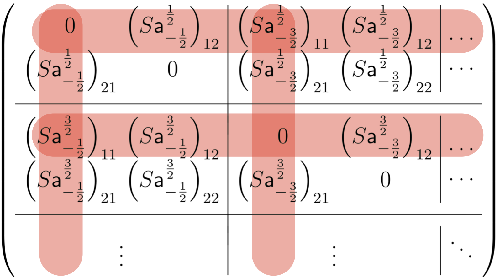
(a) Pfaffian minor of the antisymmetric $2\times 2$ block infinite matrix $S{\sf a}$ associated to the pair of strict partitions $\vec{\lambda}_{1}=\left((1,0),\emptyset\right)$.
$\mathrm{Pf}\left(S{\sf a}\right)_{\vec{\lambda}_{1}}=\mathrm{Pf}\left(\begin{array}[]{cc}0&\left(S{\sf a}^{\frac{1}{2}}_{-\frac{3}{2}}\right)_{11}\\ \left(S{\sf a}^{\frac{3}{2}}_{-\frac{1}{2}}\right)_{11}&0\end{array}\right)$.

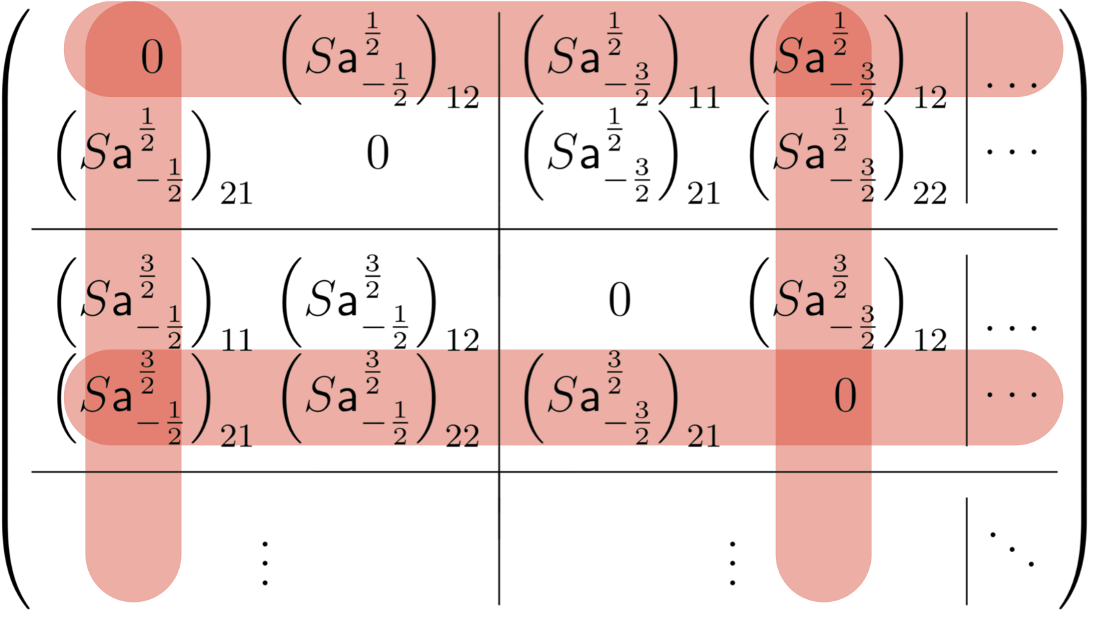
(b) Pfaffian minor of the antisymmetric $2\times 2$ block infinite matrix $S{\sf a}$, associated to the pair of strict partitions $\vec{\lambda}_{2}=\left((0),(1)\right)$.

$\mathrm{Pf}\left(S{\sf a}\right)_{\vec{\lambda}_{2}}=\mathrm{Pf}\left(\begin{array}[]{cc}0&\left(S{\sf a}^{\frac{1}{2}}_{-\frac{3}{2}}\right)_{12}\\ \left(S{\sf a}^{\frac{3}{2}}_{-\frac{1}{2}}\right)_{21}&0\end{array}\right)$.

Figure 2: $2\times 2$ Pfaffian minors of the infinite antisymmetric block matrix $S{\sf a}$. The strict partitions label the rows and columns.

5 Pfaffian $\tau$-function and the orthogonal Drinfeld-Sokolov hierarchy

We turn to a first application of the results of Section 4.2 and our general formalism. This will allow us to write the $\tau$-function for the Drinfeld-Sokolov hierarchy [9] as a Pfaffian, as well as providing an expansion in terms of Pfaffian minors labeled by $N$-tuples of strict partitions, where $N=2\ell+1$ for the $B_{\ell}^{(1)}$ case and $N=2\ell$ for the $D_{\ell}^{(1)}$ case.

First recall some standard notation for affine Kac-Moody algebras. Let $\ell$ be the rank of the Lie algebra $\mathfrak{g}=\mathfrak{so}_{N}$, where either $N=2\ell+1$, for $B_{\ell}$ or $N=2\ell$ for $D_{\ell}$, let $\mathfrak{h}\subset\mathfrak{so}_{N}$ be a Cartan subalgebra, and $\Pi:=\{\alpha_{1},\dots,\alpha_{\ell}\}$ a set of simple roots. If $\Delta\subset\mathfrak{h}^{*}$ is the root system, we have the decomposition

$$\mathfrak{g}=\mathfrak{h}\bigoplus_{\alpha\in\Delta}\mathfrak{g}_{\alpha}.$$ (5.1)

For $\alpha\in\Delta$, let $h_{\alpha}\in\mathfrak{h}$ be defined by

$$B\left(h_{\alpha},X\right)=\alpha(X),\quad\forall\ X\in\mathfrak{h},$$ (5.2)

where $B$ is the Killing form, and

$$H_{\alpha}:=\frac{2h_{\alpha}}{B(h_{\alpha},h_{\alpha})}.$$ (5.3)

Define the $\mathrm{ad}^{*}$ and Weyl group invariant bilinear form $(\,\cdot\,|\,\cdot\,)$ on $\mathfrak{h}^{*}$ by

$$\left(\alpha|\beta\right):=\kappa\,B\left(H_{\alpha},H_{\beta}\right),\quad\forall\ \alpha,\beta\in\Delta,$$ (5.4)

where $\kappa$ is determined by requiring

$$\left(\theta|\theta\right)=2$$ (5.5)

for the highest root $\theta$ with respect to $\Pi$. Let

$$E_{i}\in\mathfrak{g}_{\alpha_{i}},\quad F_{i}\in\mathfrak{g_{-\alpha_{i}}},\quad H_{i}:=\frac{2H_{\alpha_{i}}}{\left(\alpha_{i}|\alpha_{j}\right)},\\$$ (5.6)

be a set of Weyl generators of $\mathfrak{g}$, satisfying

$$[H_{i},E_{j}]=A_{ij}E_{j},\quad[H_{i},F_{j}]=-A_{ij}F_{j},\quad[E_{i},F_{j}]=H_{i}\delta_{ij},\quad i,j=1,\dots,\ell,$$ (5.7)

where $A_{ij}$ is the Cartan matrix. Define the Chevalley involution $\SS$ by

$$\SS(E_{i})=-F_{i},\quad\SS(F_{i})=-E_{i},\quad\SS(H_{i})=-H_{i},\quad i=1,\dots,\ell,$$ (5.8)

extended as an involutive automorphism of the algebra. Fix $E_{-\theta}\in\mathfrak{g}_{-\theta}$, $E_{\theta}\in\mathfrak{g}_{\theta}$ by the conditions

$$\left(E_{\theta}|E_{-\theta}\right)=1,\quad\SS(E_{-\theta})=-E_{\theta},$$ (5.9)

and define

$$E_{0}:=E_{-\theta},\quad F_{0}:=E_{\theta},\quad H_{0}:=[E_{0},F_{0}].$$ (5.10)

A set of Weyl generators for the affine Kac-Moody algebra $\mathfrak{g}^{(1)}$, obained as a central extension of the loop algebra $L\mathfrak{g}$ is

$$e_{i}:=z^{\delta_{i,0}}E_{i},\quad f_{i}:=z^{-\delta_{i,0}}F_{i},\quad h_{i}:=H_{i}.$$ (5.11)

We use the matrix realization of $L_{S}\mathfrak{so}(N)$ introduced in [9, 23, 7], which is recalled in Appendix B. In this representation, elements of the Lie algebra satisfy

$$X^{t}=-SXS=-\mathcal{S}(X),$$ (5.12)

where $S$ is the matrix representation of the Chevalley involution, acting by conjugation, defined in eqs. (B.7) and (B.15).) We introduce the shift matrix

$$\Lambda:=\sum_{i=1}^{n}E_{i}+zE_{-\theta}\in L_{+}\mathfrak{g},$$ (5.13)

satisfying

$$\Lambda^{1+h}=z\Lambda,$$ (5.14)

where

$$h=\begin{cases}2\ell=N-1,&\ \text{for }\ B_{\ell}^{(1)},\\ 2\ell-2=N-2,&\ \text{for }\ D_{\ell}^{(1)}\end{cases}$$ (5.15)

is the Coxeter number. The time evolution of the corresponding Drinfeld-Sokolov hierarchy is encoded in $\Psi_{+}(z)\in L_{S+}SO(N)$, defined by:

$$\Psi_{+}(z):=e^{Y(z,\mathbf{t}_{0})},\quad Y(z,\mathbf{t}_{0}):=\left\{\sum_{k=1}^{\infty}t_{2k+1}\Lambda^{2k+1}\right\}.$$ (5.16)

where

$$\mathbf{t}_{0}:=(t_{1},t_{3},t_{5},\dots).$$ (5.17)

The initial condition is encoded in an arbitrary negative element $\Psi_{-}\in L_{S-}SO(N)$, which we write as

$$\Psi_{-}(z):=e^{-X(z)},\quad X(z)\in L_{S-}\mathfrak{so}(N).$$ (5.18)

In [5] it was shown that the Widom constant (3.6) is the square of the $\tau$-function of the Drinfeld-Sokolov hierarchy with time evolution defined by (5.16) and initial condition specified by (5.18), namely:

$$\tau_{W}[J]=\tau_{DS}^{2}.$$ (5.19)

Equation (5.19) is already a strong indication that $\tau_{DS}$ should be a Pfaffian, since it is the square root of the Widom constant $\tau$-function $\tau_{W}[J]$. In fact, this is a special instance of Theorem (4.2), following from (5.12), which means that both $\Psi_{+},\Psi_{-}$ satisfy our orthogonal loop group condition (3.11):

Proposition 5.1.

The $\tau$-function of the Drinfeld-Sokolov hierarchy of type $D_{\ell}^{(1)}$ or $B_{\ell}^{(1)}$ is the Pfaffian expression (4.44), where $S$ is the Chevalley involution of the appropriate loop algebra, where $\Psi_{+}(z)$ entering in ${\sf a}(z,w)$ is given by (5.16), and $\Psi_{-}(z)$ by (5.18) where $X_{-}$ is an arbitrary element of $L_{S}\mathfrak{so}(N)$.

It follows from Proposition (5.1) that we have combinatorial expansions of the $\tau$-functions as in (4.55), which we write here for convenience:

$$\tau_{DS}=\sum_{\vec{\lambda}\in SP}\mathrm{Pf}({\sf a}_{\vec{\lambda}})\mathrm{Pf}({\sf d}_{\vec{\lambda}}).$$ (5.20)

The term term $\mathrm{Pf}({\sf d}_{\vec{\lambda}})$ in this context gives the Cartan coordinate of the point in the (isotropic) Grassmannian for $L_{S}\operatorname{SO}(N)$ corresponding to the given initial condition and to the $N$-tuple of strict partitions $\vec{\lambda}$, while the term $\mathrm{Pf}({\sf a}_{\vec{\lambda}})$ specifies the time dependence.

Remark 5.1.

Previous expressions [6, 4, 7] for Drinfeld-Sokolov $\tau$-functions were obtained by expanding the Widom $\tau$-function in minor determinants labeled by all types of partitions and then taking a square root. The expansion in terms of Pfaffians is more intrinsic, since everything is formulated directly on the isotropic Grassmannian defined by the fermions (4.29). Furthermore, it is more efficient, since the set of strict partitions is only a small subset of the full set of partitions.

6 Examples of polynomial Drinfeld-Sokolov $\tau$-functions

The simplest type of Drinfeld-Sokolov $\tau$-functions are polynomials, for which the initial condition matrix is $\Psi_{-}(z)=e^{X}(z)$ where $X(z)$ is nilpotent, so the expression for $\Psi_{-}$ truncates at finite order and ${\sf a},{\sf d}$ are effectively finite block matrices. We compute here some examples of such polynomial $\tau$-functions

6.1 $B_{1}^{(1)}$ polynomial $\tau$-function

A first example of a polynomial Drinfeld-Sokolov $\tau$-function in the case $B_{1}^{(1)}=L_{S}\operatorname{SO}(3)$, is obtained by choosing the following upper or lower triangular initial condition data:

$$X_{1}(z)=\frac{1}{z}\left(\begin{array}[]{ccc}0&0&0\\ a&0&0\\ 0&a&0\end{array}\right),\quad X_{2}(z)=\frac{1}{z}\left(\begin{array}[]{ccc}0&b&0\\ 0&0&b\\ 0&0&0\end{array}\right).$$ (6.1)

We restrict to the first three times $t_{1},t_{3},t_{5}$, and take $\Psi_{+}(z)$ in $(\ref{eq:PsipB})$ to be $e^{Y(z,\mathbf{t}_{o})}$, where

$$\begin{split}Y(z,\mathbf{t}_{o})&:=t_{1}\Lambda+t_{3}\Lambda^{3}+t_{5}\Lambda^{5}\\ &=\left(\begin{array}[]{ccc}0&\frac{1}{2}z\left(z\left[zt_{5}+t_{3}\right)+t_{1}\right]&0\\ z\left(zt_{5}+t_{3}\right)+t_{1}&0&\frac{1}{2}z\left[z\left(zt_{5}+t_{3}\right)+t_{1}\right]\\ 0&z\left(zt_{5}+t_{3}\right)+t_{1}&0,\\ \end{array}\right)\end{split},$$ (6.2)

so the factorized group element is

$$J_{a}(z):=e^{-X_{a}(z)}e^{Y(z,\mathbf{t}_{0})},\quad a=1,2.$$ (6.3)

The Cartan coordinates (the coefficients in the $Q$-Schur function expansion) and time polynomials for the initial condition matrix $\Psi_{+}(z)=e^{X_{1}(z)}$ are then

$$\vskip 3.0pt plus 1.0pt minus 1.0pt\begin{array}[]{c|c|c}\mathrm{Pf}({\sf d}_{\vec{\lambda}})&\mathrm{Pf}({\sf a}_{\vec{\lambda}})&\vec{\lambda}\\ \hline\cr-a&\frac{t_{1}}{2}=\frac{1}{2}Q_{(1,0)}(\mathbf{t}_{0})&\left(\begin{array}[]{ccc}\emptyset,&(0),&(0)\\ \end{array}\right)\\ -\frac{a^{2}}{2}&-\frac{t_{1}^{2}}{8}=-\frac{1}{4}Q_{(2,0)}(\mathbf{t}_{0})&\left(\begin{array}[]{ccc}\emptyset,&\emptyset,&(1,0)\\ \end{array}\right)\end{array}\vskip 3.0pt plus 1.0pt minus 1.0pt$$ (6.4)

and the resulting $\tau$-function is

$$\tau_{O}[J_{1}]=\left(1-a\frac{t_{1}}{4}\right)^{2}.$$ (6.5)

The Cartan coordinates and time polynomials for the initial condition matrix $e^{X_{2}(z)}$ are

$$\vskip 3.0pt plus 1.0pt minus 1.0pt\begin{array}[]{c|c|c}\mathrm{Pf}({\sf d}_{\vec{\lambda}})&\mathrm{Pf}({\sf a}_{\vec{\lambda}})&\vec{\lambda}\\ \hline\cr b&\frac{t_{1}^{3}}{12}-t_{3}=\frac{1}{2}Q_{(2,1)}(\mathbf{t}_{0})&\left(\begin{array}[]{ccc}(0),&(0),&\emptyset\\ \end{array}\right)\\ -\frac{b^{2}}{2}&-\frac{1}{288}\left(t_{1}^{3}-12t_{3}\right)^{2}=-\frac{1}{2}Q_{(4,2)}(\mathbf{t}_{0})&\left(\begin{array}[]{ccc}(1,0),&\emptyset,&\emptyset\\ \end{array}\right)\end{array},\vskip 3.0pt plus 1.0pt minus 1.0pt$$ (6.6)

and the corresponding $\tau$-function is

$$\tau_{O}[J_{2}]=\left(\frac{a}{24}\left(t_{1}^{3}-12t_{3}\right)+1\right)^{2}.$$ (6.7)

Remark 6.1.

Here the $Q_{\lambda}$’s are $Q$-Schur functions, labelled by strict partitions [27, 19]. In these examples, and others to follow, the strict partition $\lambda=\{\lambda_{j}\}$ labelling the $Q$-Schur function is obtained from the $N$-tuple of strict partitions $\vec{\lambda}=\left(\lambda^{(1)},\dots,\lambda^{(N)}\right)$ through the following (empirical) rule:

$$\{\lambda_{i}\}=\{N-\alpha+\lambda_{j}^{(\alpha)}(N-1)\}_{j=1,\dots n_{\alpha}\atop\alpha=1,\dots,N},$$ (6.8)

properly ordered. This is not an isomorphism, however, since the same combined strict partition can be obtained from more than one $N$-tuple of strict partitions. Moreover, there are, in principle, $N$-tuples of strict partitions that could lead to a combined partition that is non-strict. It seems, however, that those Pfaffian minors in which this occurs always vanish.

Remark 6.2.

Comparing with [5], eq. (4.1), the Pfaffian $\tau$-functions for the $SO(3)$ case are themselves seen to be squares of the corresponding $A_{1}^{(1)}$ Drinfeld-Sokolov polynomial $\tau$-functions with rescaled times. An explanation of this is given in Theorem 7.2.

6.2 $B_{2}^{(1)}$ polynomial $\tau$-function

We now give a much less trivial example of polynomial $\tau$-function. Specify the initial condition to be $\Psi_{-}(z)=e^{X_{3}(z)}$, where

$$X_{3}(z):=\left(\begin{array}[]{ccccc}0&0&0&0&0\\ \frac{a_{2}}{z}&0&0&0&0\\ \frac{a_{3}}{z}&\frac{a_{5}}{z}&0&0&0\\ \frac{a_{4}}{z}&0&\frac{a_{5}}{z}&0&0\\ 0&\frac{a_{4}}{z}&-\frac{a_{3}}{z}&\frac{a_{2}}{z}&0\\ \end{array}\right),$$ (6.9)

and the time evolution factor to be $\Psi_{+}(z)=e^{Y_{3}(z,\mathbf{t}_{o})}$, where

$$Y_{3}(z,\mathbf{t}_{o}) {\hskip-20.0pt}:=t_{1}\Lambda+t_{3}\Lambda^{3}+t_{5}\Lambda^{5}$$ (6.17)

$${\hskip-20.0pt}=\left(\begin{array}[]{ccccc}0&-\frac{1}{2}zt_{3}&0&-\frac{1}{2}\left(z^{2}t_{5}+zt_{1}\right)&0\\ -(zt_{5}+t_{1})&0&-zt_{3}&0&-\frac{1}{2}\left(z^{2}t_{5}+zt_{1}\right)\\ 0&-(zt_{5}+t_{1})&0&-zt_{3}&0\\ -t_{3}&0&-(zt_{5}+t_{1})&0&-\frac{1}{2}zt_{3}\\ 0&-t_{3}&0&-(zt_{5}+t_{1})&0\\ \end{array},\right)$$

so

$$J_{3}(z):=e^{-X_{3}(z)}e^{Y_{3}(z,\mathbf{t}_{0})}.$$ (6.19)

In this case, there are many more nonzero Cartan coordinates. For readability, we tabulate them, and the corresponding time dependant polynomial, only up to weights $|\lambda^{\alpha)}|=4$, in Appendix A

The expressions for coloured strict partitions of higher order become very long, so we do not write them down explicitly. Remarkably, all the time polynomials are again multiples of $Q$-Schur polynomials, which are tabulated, together with their coefficients, in Appendices A.2 and A.1 for 5-tuples $\vec{\lambda}$ of strict partitions of lengths $\ell(\lambda^{\alpha})\leq 4$. The $\tau$-function is a polynomial of degree 30, which is too long to write in detail for the general case. However, setting e.g. $a_{2}=0$ considerably simplifies the expression, which becomes

$$\begin{split}\tau_{0}[J_{3}]&=1+\frac{a_{4}t_{1}}{2}+\frac{1}{4}a_{3}t_{1}^{2}-\frac{1}{12}a_{5}t_{1}^{3}-\frac{1}{192}a_{3}^{2}t_{1}^{4}+\frac{1}{192}a_{3}a_{5}t_{1}^{5}-\frac{1}{720}a_{5}^{2}t_{1}^{6}\\ &+a_{5}t_{3}-\frac{1}{8}a_{3}^{2}t_{3}t_{1}+\frac{1}{8}a_{3}a_{5}t_{3}t_{1}^{2}-\frac{1}{24}a_{5}^{2}t_{3}t_{1}^{3}+\frac{1}{4}a_{5}^{2}t_{3}^{2}+\frac{1}{4}a_{5}^{2}t_{5}t_{1}.\end{split}$$ (6.20)

6.3 $D_{4}^{(1)}$ polynomial $\tau$-function

We conclude our list of examples with a simple polynomial $\tau$-function for the $D_{\ell}^{(1)}$ series, choosing the case of $SO(8)$. Since the size of the matrices starts to be quite large, we consider here the simplest lower triangular initial condition, and as before we consider time evolution with respect to $t_{1},t_{3},t_{5}$:  choosing

$$X_{4}(z)=\frac{1}{z}\left(\begin{array}[]{cccccccc}0&0&0&0&0&0&0&0\\ 0&0&0&0&0&0&0&0\\ 0&0&0&0&0&0&0&0\\ 0&0&0&0&0&0&0&0\\ 0&0&0&0&0&0&0&0\\ 0&0&0&0&0&0&0&0\\ a&0&0&0&0&0&0&0\\ 0&a&0&0&0&0&0&0\end{array}\right), Y_{4}(z,\mathbf{t}_{o})=z\left(\begin{array}[]{cccccccc}0&\frac{t_{5}}{2}&0&\frac{t_{3}}{4}&\frac{t_{3}}{2}&0&\frac{t_{1}}{2}&0\\ t_{1}&0&t_{5}&0&0&t_{3}&0&\frac{t_{1}}{2}\\ 0&t_{1}&0&\frac{t_{5}}{2}&t_{5}&0&t_{3}&0\\ t_{3}&0&t_{1}&0&0&t_{5}&0&\frac{t_{3}}{2}\\ \frac{t_{3}}{2}&0&\frac{t_{1}}{2}&0&0&\frac{t_{5}}{2}&0&\frac{t_{3}}{4}\\ 0&t_{3}&0&\frac{t_{1}}{2}&t_{1}&0&t_{5}&0\\ t_{5}&0&t_{3}&0&0&t_{1}&0&\frac{t_{5}}{2}\\ 0&t_{5}&0&\frac{t_{3}}{2}&t_{3}&0&t_{1}&0\\ \end{array}\right).$$ (6.37)

with

$$J_{4}(z):=e^{-X_{4}(z)}e^{Y_{4}(z,\mathbf{t}_{0})}$$ (6.38)

The only nontrivial Cartan coordinate is

$$\mathrm{Pf}\left({\sf d}_{\left((0),(0),(0),(0),(0),(0),(1),(1)\right)}\right)=-a,$$ (6.39)

so we only need

$$\mathrm{Pf}\left({\sf a}_{\left((0),(0),(0),(0),(0),(0),(1),(1)\right)}\right)=\frac{t_{1}}{2}=\frac{1}{2}Q_{(1,0)}(\mathbf{t}_{o}),$$ (6.40)

giving

$$\tau_{O}[J_{4}]=1-a\frac{t_{1}}{2}.$$ (6.41)

7 $SO(N)$ linear systems and their isomonodromic deformations

Another important class of problems for which the $\tau$-function has been identified with a Widom constant (3.6) are the isomonodromic deformations of $SL(N)$ linear systems of ODEs on the Riemann sphere with punctures [4]. In the following, we show how the RH problem may be defined, in the case of four simple poles, and how the general solution for the $\operatorname{SO}(3)$ case may be deduced from the corresponding results derived in [4] for the $SL(2)$ case, corresponding to Painlevé’s sixth transcendant $P_{VI}$.

7.1 4-point $\mathfrak{g}$-valued linear system and the Widom $\tau$-function

We illustrate first how to generalize the known construction for $SL(N)$ to the case of an arbitrary matrix representation $\rho$ of a Lie algebra $\mathfrak{g}$ corresponding to a semisimple Lie group $G$, by considering the explicit example of a Fuchsian system with four singular points $0,t,1,\infty$:

$$\partial_{z}\Phi(z)=\Phi(z)A(z),\quad A(z)=\frac{A_{0}}{z}+\frac{A_{t}}{z-t}+\frac{A_{1}}{z-1},$$ (7.1)

where $A_{0},A_{t},A_{1}$ are $N\times N$ matrices in the representation $\rho$. The case of a more general linear systems on the sphere with rational coefficients can be studied by similar means following the construction of [4], Section 3.

In the generic case, the matrices $A_{0},A_{t},A_{1}$ can be written as

$$A_{k}=G_{k}\Theta_{k}G_{k}^{-1},\quad k=0,t,1,$$ (7.2)

where $G_{k}\in G$ and $\Theta_{k}\in\mathfrak{h}$, the Cartan subalgebra of $\mathfrak{g}$. The local solution of this linear system around the singular points will be

$$\Phi^{(k)}(z)=\begin{cases}(z_{k}-z)^{\Theta_{k}}G^{(k)}(z),&k=0,1,t,\\ (-z)^{-\Theta_{\infty}}G^{(\infty)}(z),\end{cases}$$ (7.3)

where $G^{(k)}(z)\in LG$ are holomorphic matrix functions in a neighborhood of the singular point, such that $G^{(k)}(z_{k})=G_{k}$. Around the singular points of the equation, $\Phi(z)$ will have monodromies

$$M_{k}=G_{k}e^{2\pi i\Theta_{k}}G_{k}^{-1},\quad k=0,1,t, M_{0}M_{t}M_{1}M_{\infty}=\mathbb{I}_{n}.$$ (7.4)

Now define $\mathfrak{S}$ through

$$e^{2\pi i\mathfrak{S}}:=M_{0}M_{t},$$ (7.5)

which generically can be assumed to lie in the Cartan subalgebra of the Lie algebra (if needed, by applying a constant gauge transformation to the linear system (7.1)). $\mathfrak{S}$ in (7.5) is defined only up to shifts in the root lattice $\mathcal{Q}(\mathfrak{g})$. Let $D_{a}$, $a=0,1,t$ be small discs surrounding the points $0,1,t$, and assume for convenience that $0<|t|<1$. Consider the contour $\Gamma$ shown in Figure 3(a). It divides the Riemann sphere with the points $0,t,1,\infty$ removed into two regions, which we call $\mathcal{T}_{\pm}$, corresponding geometrically to a decomposition of the four-punctured sphere into two pairs of pants which we identify with the regions $\mathcal{T}_{\pm}$, as in Figure 3(b). The circle $\mathcal{C}$ of radius $R$, centered at the origin, along which the pants are glued is identified as the red circle of Figure 3, with $|t|<R<1$.

(a) The black solid lines constitute the RHP contour $\Gamma$, dividing the complex plane in two regions $\mathcal{T}_{\pm}$.

(b) Pants decomposition of four-punctured sphere corresponding to the contour $\Gamma$. The two pants are glued along the circle $\mathcal{C}$.

Figure 3:

To a fundamental matrix solution of (7.1) we can associate a piecewise defined function

$$\Psi(z):=\begin{cases}G^{(a)}(z),&z\in D_{a},\quad,a=0,1,t,\\ \Phi(z),&z\in\mathcal{T}_{-}\cup\mathcal{T}_{+},\,z\notin,\Gamma,\\ (-z)^{\mathfrak{S}}\Phi(z),&z\notin\Gamma.\end{cases}$$ (7.6)

This function solves a dual RHP (i.e. with appropriate jumps factorized as in (3.4)) on $\Gamma$, which we do not specify since they will not be needed in the following (see [14, 4] for further details).

To apply the Widom constant formalism, we need to reduce this dual Riemann-Hilbert problem to a direct Riemann-Hilbert problem on a circle with factorization as in (3.3), written in terms of known functions $\Psi_{\pm}$. To do this, consider the solutions $\Phi_{\pm}$ of two auxiliary 3-point Fuchsian linear systems on the two trinions (i.e. pairs of pants, obtained by replacing the three punctures at the poles by oval boundaries).

$$\partial_{z}\Phi_{-}(z)=\Phi_{-}(z)A_{-}(z)\quad A_{-}(z)=\frac{A_{0,-}}{z}+\frac{A_{t,-}}{z-t},$$

$$\partial_{z}\Phi_{+}(z)=\Phi_{+}(z)A_{+}(z)\quad A_{+}(z)=\frac{A_{0,+}}{z}+\frac{A_{1,+}}{z-1},$$ (7.7)

where $A_{k,\pm}\sim\Theta_{k}$ are $N\times N$ matrices in the representation $\rho$ of $\mathfrak{g}$, normalized as

$$\Phi_{+}(z)\simeq(-z)^{\mathfrak{S}},\quad z\rightarrow 0, \Phi_{-}(z)\simeq(-z)^{\mathfrak{S}},\quad z\rightarrow\infty.$$ (7.8)

By restricting the dual RHP to the pants $\mathcal{T}_{\pm}$ in Figure 3 we obtain two solutions $\Psi_{\pm}$ of two three-point problems, which on the circle $\mathcal{C}$ are related to $\Phi_{\pm}$ by

$$\Psi_{\pm}(z)=(-z)^{-\mathfrak{S}}\Phi_{\pm}(z),\qquad z\in\mathcal{C}.$$ (7.9)

Since $\Psi_{\pm}$ have the same jumps as $\Psi$ inside the trinions $\mathcal{T}_{\pm}$ respectively, the function

$$\bar{\Psi}(z):=\begin{cases}\Psi_{+}(z)^{-1}\Psi(z):=\bar{\Psi}_{-}(z),&\text{outside }\mathcal{C},\\ \Psi_{-}(z)^{-1}\Psi(z):=\bar{\Psi}_{+}(z),&\text{inside }\mathcal{C}\end{cases}$$ (7.10)

is single-valued everywhere apart from the circle $\mathcal{C}$, where it has a jump admitting the two factorizations

$$J(z)=\bar{\Psi}_{+}(z)\bar{\Psi}_{-}(z)^{-1}=\Psi_{-}(z)^{-1}\Psi_{+}(z).$$ (7.11)

In [4] it was shown that the Widom $\tau$-function (3.6), with kernel written in terms of the functions $\Psi_{\pm}$ defined above, is related to the JMU $\tau$-function for the linear system (7.1), defined by

$$\partial_{t}\log\tau_{JMU}^{\mathrm{SL}(N)}=\frac{1}{2}\mathop{\mathrm{res}}\limits_{z=t}\mathrm{tr}A(z)^{2}=\frac{\mathrm{tr}A_{0}A_{t}}{t}+\frac{A_{t}A_{1}}{t-1},$$ (7.12)

in the following way:

$$\tau_{JMU}^{\mathrm{SL}(N)}(t)=\text{const.}\,t^{\frac{1}{2}\mathrm{tr}\left(\mathfrak{S}^{2}-\Theta_{0}^{2}-\Theta_{t}^{2}\right)}\tau_{W}(t).$$ (7.13)

Although the proof in [4], based on comparing the logarithmic $t$-derivative of $\tau_{W}$ to (7.12), was given only for the $\mathrm{SL}(N)$ case, it applies to this more general context without any modification, if the RHP is formulated analogously to the above. For an arbitrary classical Lie group $G$, the definition of the JMU $\tau$-function can be expressed as

$$\partial_{t}\log\tau_{\mathrm{JMU}}^{G}=\frac{\kappa}{2}\mathop{\mathrm{res}}\limits_{z=t}\mathrm{tr}\left(A(z)^{2}\right),$$ (7.14)

where $\kappa=1$ for $\mathrm{SL}(N)$ and $\operatorname{Sp}(N)$ and $\kappa=\frac{1}{2}$ for $SO(N)$. Specializing to $SO(N)$, we have

$$\begin{split}\partial_{t}\log\tau_{\mathrm{JMU}}^{SO(N)}&=\frac{1}{4}\mathop{\mathrm{res}}\limits_{z=t}\mathrm{tr}A(z)^{2}=\frac{\mathrm{tr}A_{0}A_{t}}{2t}+\frac{A_{t}A_{1}}{2(t-1)}=\frac{1}{2}\partial_{t}\log\left(t^{\frac{1}{2}\mathrm{tr}\left(\mathfrak{S}^{2}-\Theta_{0}^{2}-\Theta_{t}^{2}\right)}\tau_{W}(t)\right)\\ &=\partial_{t}\log\left(t^{\frac{1}{4}\mathrm{tr}\left(\mathfrak{S}^{2}-\Theta_{0}^{2}-\Theta_{t}^{2}\right)}\tau_{O}[J](t)\right),\end{split}$$ (7.15)

and

$$\tau_{\mathrm{JMU}}^{SO(N)}=\text{const.}\,t^{\frac{1}{4}\mathrm{tr}\left(\mathfrak{S}^{2}-\Theta_{0}^{2}-\Theta_{t}^{2}\right)}\tau_{O}[J].$$ (7.16)

This may be generalized to an arbitrary number of Fuchsian singularities, or to irregular singularities of higher Poincaré rank at $0$ and $\infty$, following the $\mathrm{SL}(N)$ construction of [4].

7.2 The $SO(3)$ isomonodromic $\tau$-function

In the case of an $\mathrm{SL}(2,\mathbb{C})$ linear system, it is well-known that the solution to the 3-point problem can be written explicitly in terms of hypergeometric functions ${}_{2}F_{1}$. We recall the expressions for the solution of the corresponding $\mathrm{SL}(2)$ RHP, which we denote by $\Psi_{\pm}^{(2)}$, from [14]:

$$\begin{split}\Psi^{(2)}_{+}(z)&=\left(\begin{array}[]{cc}{}_{1}F_{2}{\left[\genfrac{.}{.}{0.0pt}{}{\theta_{1}+\theta_{\infty}+\sigma{\mathchar 44\relax}\mskip 8.0mu\theta_{1}-\theta_{\infty}+\sigma}{2\sigma};z\right]}&z\frac{\theta_{\infty}^{2}-(\theta_{1}+\sigma)^{2}}{2\sigma(1+2\sigma)}{}_{1}F_{2}{\left[\genfrac{.}{.}{0.0pt}{}{1+\theta_{1}+\theta_{\infty}+\sigma{\mathchar 44\relax}\mskip 8.0mu1+\theta_{1}-\theta_{\infty}+\sigma}{2+2\sigma};z\right]}\\ -z\frac{\theta_{\infty}^{2}-(\theta_{1}-\sigma)^{2}}{2\sigma(1-2\sigma)}{}_{1}F_{2}{\left[\genfrac{.}{.}{0.0pt}{}{1+\theta_{1}+\theta_{\infty}-\sigma{\mathchar 44\relax}\mskip 8.0mu1+\theta_{1}-\theta_{\infty}-\sigma}{2-2\sigma};z\right]}&{}_{1}F_{2}{\left[\genfrac{.}{.}{0.0pt}{}{\theta_{1}+\theta_{\infty}-\sigma{\mathchar 44\relax}\mskip 8.0mu\theta_{1}-\theta_{\infty}-\sigma}{-2\sigma};z\right]}\end{array}\right)\\ &:=\left(\begin{array}[]{cc}K_{++}(z)&K_{+-}(z)\\ K_{-+}(z)&K_{--}(z)\end{array}\right).\end{split}$$ (7.17)

$$\begin{split}\Psi^{(2)}_{-}(z)&=\left(\begin{array}[]{cc}{}_{1}F_{2}{\left[\genfrac{.}{.}{0.0pt}{}{\theta_{t}+\theta_{0}-\sigma{\mathchar 44\relax}\mskip 8.0mu\theta_{t}-\theta_{0}-\sigma}{-2\sigma};\frac{t}{z}\right]}&-t^{-2\sigma}e^{-i\eta}\frac{t}{z}\frac{\theta_{0}^{2}-(\theta_{t}-\sigma)^{2}}{2\sigma(1-2\sigma)}{}_{1}F_{2}{\left[\genfrac{.}{.}{0.0pt}{}{1+\theta_{t}+\theta_{0}-\sigma{\mathchar 44\relax}\mskip 8.0mu1+\theta_{t}-\theta_{0}-\sigma}{2-2\sigma};\frac{t}{z}\right]}\\ t^{2\sigma}e^{i\eta}\frac{t}{z}\frac{\theta_{0}^{2}-(\theta_{t}+\sigma)^{2}}{2\sigma(1+2\sigma)}{}_{1}F_{2}{\left[\genfrac{.}{.}{0.0pt}{}{1+\theta_{t}+\theta_{0}+\sigma{\mathchar 44\relax}\mskip 8.0mu1+\theta_{t}-\theta_{0}+\sigma}{2+2\sigma};\frac{t}{z}\right]}&{}_{1}F_{2}{\left[\genfrac{.}{.}{0.0pt}{}{\theta_{t}+\theta_{0}+\sigma{\mathchar 44\relax}\mskip 8.0mu\theta_{t}-\theta_{0}+\sigma}{2\sigma};\frac{t}{z}\right]}\end{array}\right)\\ &:=\left(\begin{array}[]{cc}\widetilde{K}_{++}(z)&\widetilde{K}_{+-}(z)\\ \widetilde{K}_{-+}(z)&\widetilde{K}_{--}(z)\end{array}\right).\end{split}.$$ (7.18)

While the $SO(3)$ $3$-point linear system might at first seem harder to solve, we can still express its solution in terms of hypergeometric functions, simply by changing the representation.

Proposition 7.1.

Let $\Phi^{(2)}(z)$ be the solution to the $2\times 2$ linear system

$$\partial_{z}\Phi^{(2)}(z)=\Phi^{(2)}(z)A^{(2)}(z),\quad A(z)=\sum_{\alpha=1}^{3}A^{\alpha}(z)\sigma_{\alpha},$$ (7.19)

where $A^{a}(z)$ are rational functions and $\{\sigma_{\alpha}\}_{\alpha=1,2,3}$ are the Pauli matrices. The $3\times 3$ matrix $\Phi(z)$ with components

$$\Phi_{\alpha\beta}(z)=\frac{1}{2}\mathrm{tr}\left(\sigma_{i}\Phi^{(2)}(z)\sigma_{j}\Phi^{(2)}(z)^{-1}\right),\quad\alpha,\beta=1,\dots,3$$ (7.20)

satisfies $\Phi(z)\Phi(z)^{t}=\mathbb{I}_{3}$ and solves the $3\times 3$ linear system with rational coefficients

$$\partial_{z}\Phi(z)=\Phi(z)A^{(3)}(z),\quad A^{(3)}(z)=-2i\sum_{\alpha=1}^{3}A^{\alpha}(z)J_{\alpha},$$ (7.21)

where we have introduced the $SO(3)$ generators

$$(J_{\alpha})_{\beta\gamma}=\epsilon_{\alpha\beta\gamma}.$$ (7.22)

Proof.

This follows from the isomorphism between representations of $\mathrm{SL}(2)$ and $SO(3)$ which t can be verified directly using the Euler angle representation

$$\Phi^{(2)}(z)=e^{\varphi_{1}(z)\sigma_{3}}e^{\varphi_{2}(z)\sigma_{2}}e^{\varphi_{3}(z)\sigma_{3}},$$ (7.23)

which allows us to verify (7.21) by explicit computation. ∎

Proposition 7.1 gives a way to compute the $\tau$-function for the $SO(3)$ $4$-point isomonodromic problem; just transform the $\mathrm{SL}(2)$ solutions $\Psi_{\pm}^{(2)}$ into $SO(3)$ solutions $\Psi_{\pm}^{(3)}$ using (7.1), which then can be used to define the Pfaffian $\tau$-function (4.66) through the operators ${\sf a},{\sf d}$ defined in eqs. (3.8). The resulting $3\times 3$ kernels will have explicit expressions in terms of bilinear combinations of hypergeometric functions. Proposition 7.1 allows us to write an explicit Pfaffian $\tau$-function whenever the corresponding $\mathrm{SL}(2)$ kernel entering in the Widom $\tau$-function is known. This includes the case of Painlevé $VI$ or $III$ equations, as well as the $\mathrm{SL}(2)$ Schlesinger system [14, 15, 4].

In fact, there is an even more direct relation between the $SO(3)$ $\tau$-function and the $\mathrm{SL}(2)$ $\tau$-function:

Theorem 7.2.

Let $\tau_{W}[J^{(2)}]$ be the Widom $\tau$-function (3.6), associated to a Riemann-Hilbert problem on a circle with jump $J^{(2)}(z)$, admitting direct and dual factorizations

$$J^{(2)}(z)=\Psi_{-}^{(2)}(z)^{-1}\Psi_{+}^{(2)}(z)=\bar{\Psi}^{(2)}_{+}(z)\bar{\Psi}^{(2)}_{-}(z)^{-1}\in L\mathrm{SL}(2),$$ (7.24)

and let $\tau_{O}[J^{(3)}]$ be the $SO(3)$ $\tau$-function (4.44), associated to a RHP whose solution is obtained from (7.24) through the map (7.20). Then

$$\tau_{O}[J^{(3)}]=\left(\tau_{W}[J^{(2]}]\right)^{2}.$$ (7.25)

Proof.

If $\xi$ is any parameter (which can be an isospectral or isomonodromic time, or a monodromy coordinate) that $J^{(2)}$ depends upon, the Widom $\tau$-function satisfies (see Theorem 2.3 in [4]):

$$\partial_{\xi}\log\tau_{W}[J^{(2)}]=\frac{1}{2\pi i}\oint_{S^{1}}\mathrm{tr}\left\{J^{(2)}(z)^{-1}\partial_{\xi}J^{(2)}(z)\left[\partial_{z}\bar{\Psi}^{(2)}_{-}(z)\bar{\Psi}_{-}^{(2)}(z)^{-1}+\Psi_{+}^{(2)}(z)^{-1}\partial_{z}\Psi_{+}^{(2)}(z)\right]\right\}dz.$$ (7.26)

On the other hand, the $\tau$-function $\tau_{O}[J_{3}]$ will satisfy

$$\partial_{\xi}\log\tau_{O}[J^{(3)}]=\frac{1}{4\pi i}\oint_{S^{1}}\mathrm{tr}\left\{J^{(3)}(z)^{-1}\partial_{\xi}J^{(3)}(z)\left[\partial_{z}\bar{\Psi}^{(3)}_{-}(z)\bar{\Psi}_{-}^{(3)}(z)^{-1}+\Psi_{+}^{(3)}(z)^{-1}\partial_{z}\Psi_{+}^{(3)}(z)\right]\right\}dz.$$ (7.27)

The theorem follows from the relation

$$\begin{split}&\mathrm{tr}\left\{J^{(3)}(z)^{-1}\partial_{t}J^{(3)}(z)\left[\partial_{z}\bar{\Psi}^{(3)}_{-}(z)\bar{\Psi}_{-}^{(3)}(z)^{-1}+\Psi_{+}^{(3)}(z)^{-1}\partial_{z}\Psi_{+}^{(3)}(z)\right]\right\}\\ &=4\mathrm{tr}\left\{J^{(2)}(z)^{-1}\partial_{t}J^{(2)}(z)\left[\partial_{z}\bar{\Psi}^{(2)}_{-}(z)\bar{\Psi}_{-}^{(2)}(z)^{-1}+\Psi_{+}^{(2)}(z)^{-1}\partial_{z}\Psi_{+}^{(2)}(z)\right]\right\},\end{split}$$ (7.28)

which implies that for any arbitrary parameter $\xi$ on which the $\tau$-function depends, we have

$$\partial_{\xi}\log\tau_{O}[J^{(3)}]=2\partial_{\xi}\log\tau_{W}[J^{(2)}].$$ (7.29)

∎

As an application of this theorem, using equations (7.12), (7.16), we obtain the isomonodromic $\tau$-function for the 4-point Fuchsian system on the sphere as the square of the Painlevé VI $\tau$-function. This also explains the remark made at the end of Section 6.1, that the Drinfeld-Sokolov polynomial $\tau$-functions of $B_{1}^{(1)}$ are squares of the corresponding $\tau$-functions of $A_{1}^{(1)}$.

8 Summary and future directions

We have shown that Widom $\tau$-functions derived from Riemann-Hilbert problems in orthogonal loop groups have Pfaffian rather than determinantal expressions, and provided an explicit formula (4.55) for their combinatorial expansion. Using the same methods one could study other types of Drinfeld-Sokolov $\tau$-functions, such as topological $\tau$-functions of Kontsevich-Witten type in the orthogonal case [11, 26]. It remains to find a deeper explanation for the appearance of $Q$-Schur functions in the expansions, which suggests a relation to the BKP hierarchy [21, 19] through a suitable reduction procedure.

Computing the combinatorial expansion of $SO(N)$ isomonodromic $\tau$-function should yield an orthogonal variant of the “Kiev formula” [14, 13, 8], expressing isomonodromic $\tau$-functions for $\mathrm{SL}(N)$ linear systems in terms of conformal blocks of a $W(\mathfrak{sl}_{N})$ algebra. The natural analogue would be conformal blocks of $W(\mathfrak{so}_{N})$ algebras, for which no expression is available in the case of generic monodromies (see, however, [2] for $\mathfrak{so}_{N}$ quasi-permutation monodromies, and [3] for nonautonomous Toda chains).

Another interesting variant would be the case of Riemann-Hilbert problems taking values in twisted loop groups, using multicomponent neutral fermions. Problems of this type appear in the study of Frobenius manifolds and topological quantum field theories [10, 12].

Appendix A Appendix. A polynomial $\tau$-function of $B^{(1)}_{2}$ type

Recall equation (4.33) in the main text, representing the map between decreasing sequences of positive half-integers $\{p_{\alpha,i}\}_{i=1}^{n_{\alpha}}$ and strict partitions

$$\lambda^{(\alpha)}=\left(p_{\alpha,1}-\frac{1}{2},\dots,p_{\alpha,n_{\alpha}}-\frac{1}{2}\right).$$ (A.1)

In the tables below we group the coefficients in the Pfaffian minor expansions by the total weight of the $N$-tuple of (positive) strict partitions obtained by adding $1$ to each part:

$$|\vec{\lambda}|:=\sum_{\alpha=1}^{N}\sum_{i=1}^{n_{\alpha}}(p_{\alpha,i}+\frac{1}{2}),$$ (A.2)

counting the overall power of $z$ (resp. $z^{-1}$) in the Fourier expansion of ${\sf a}$ (respectively ${\sf d}$) that contribute to the Pfaffian minor. For example

$$\mathrm{Pf}\left(\begin{array}[]{cc}0&\left(S{\sf a}^{\frac{1}{2}}_{-\frac{1}{2}}\right)_{12}\\ \left(S{\sf a}^{\frac{1}{2}}_{-\frac{1}{2}}\right)_{12}&0\end{array}\right)$$ (A.3)

has weight $|\vec{\lambda}|=2$, since it contains two Fourier coefficients of ${\sf a}$ of weight $0$ that multiply $z^{0}w^{0}$, while

$$\mathrm{Pf}\left(\begin{array}[]{cc}0&\left(S{\sf a}^{\frac{3}{2}}_{-\frac{3}{2}}\right)_{12}\\ \left(S{\sf a}^{\frac{3}{2}}_{-\frac{3}{2}}\right)_{12}&0\end{array}\right)$$ (A.4)

has weight $|\vec{\lambda}|=4$, since it contains two Fourier coefficients of ${\sf a}$ of weight $2$, that multiply $zw$.

A.1 The Pfaffian ${\sf d}$ coefficients

$$\begin{array}[]{c|c}\mathrm{Pf}({\sf d}_{\vec{\lambda}})&\vec{\lambda},\,|\vec{\lambda}|=2\\ \hline\cr-a_{2}&\left(\begin{array}[]{ccccc}\emptyset,&(0),&\emptyset,&\emptyset,&(0)\\ \end{array}\right)\\ a_{5}&\left(\begin{array}[]{ccccc}\emptyset,&\emptyset,&(0),&(0),&\emptyset\\ \end{array}\right)\\ -a_{3}&\left(\begin{array}[]{ccccc}\emptyset,&\emptyset,&(0),&\emptyset,&(0)\\ \end{array}\right)\\ -a_{4}&\left(\begin{array}[]{ccccc}\emptyset,&\emptyset,&\emptyset,&(0),&(0)\\ \end{array}\right)\\ \hline\cr\phantom{\mathrm{Pf}({\sf d}_{\vec{\lambda}})}&\vec{\lambda},\,|\vec{\lambda}|=3\\ \hline\cr\frac{a_{5}^{2}}{2}&\,\left(\begin{array}[]{ccccc}\emptyset,&\emptyset,&\emptyset,&(1,0),&\emptyset\\ \end{array}\right)\\ \frac{1}{2}\left(a_{3}^{2}-2a_{2}a_{4}\right)&\,\left(\begin{array}[]{ccccc}\emptyset,&\emptyset,&\emptyset,&\emptyset,&(1,0)\\ \end{array}\right)\\ -\frac{1}{2}a_{2}a_{5}&\,\left(\begin{array}[]{ccccc}\emptyset,&\emptyset,&(1),&\emptyset,&(0)\\ \end{array}\right)\\ \frac{a_{2}a_{5}}{2}&\,\left(\begin{array}[]{ccccc}\emptyset,&\emptyset,&(0),&\emptyset,&(1)\\ \end{array}\right)\\ -\frac{1}{2}a_{3}a_{5}&\,\left(\begin{array}[]{ccccc}\emptyset,&\emptyset,&\emptyset,&(1),&(0)\\ \end{array}\right)\\ \frac{a_{3}a_{5}}{2}&\,\left(\begin{array}[]{ccccc}\emptyset,&\emptyset,&\emptyset,&(0),&(1)\\ \end{array}\right)\\ \hline\cr\phantom{\mathrm{Pf}({\sf d}_{\vec{\lambda}})}&\vec{\lambda},\,|\vec{\lambda}|=4\\ \hline\cr-\frac{1}{6}a_{2}a_{5}^{2}&\left(\begin{array}[]{ccccc}\emptyset,&\emptyset,&\emptyset,&(2),&(0)\\ \end{array}\right)\\ -\frac{1}{6}a_{2}a_{5}^{2}&\left(\begin{array}[]{ccccc}\emptyset,&\emptyset,&\emptyset,&(0),&(2)\\ \end{array}\right)\\ \frac{1}{3}a_{2}a_{5}^{2}&\left(\begin{array}[]{ccccc}\emptyset,&\emptyset,&\emptyset,&(1),&(1)\\ \end{array}\right)\\ -a_{2}a_{5}&\left(\begin{array}[]{ccccc}\emptyset,&(0),&(0),&(0),&(0)\\ \end{array}\right)\\ \end{array}$$

A.2 The Pfaffian ${\sf a}$ coefficients

$$\begin{array}[]{c|c}\mathrm{Pf}({\sf a}_{\vec{\lambda}})&\vec{\lambda},\,|\vec{\lambda}|=2\\ \hline\cr-\frac{1}{12}\left(t_{1}^{3}+6t_{3}\right)=-\frac{1}{2}Q_{(3,0)}&\left(\begin{array}[]{ccccc}\emptyset,&(0),&\emptyset,&\emptyset,&(0)\\ \end{array}\right)\\ t_{3}-\frac{t_{1}^{3}}{12}=-\frac{1}{2}Q_{(2,1)}&\left(\begin{array}[]{ccccc}\emptyset,&\emptyset,&(0),&(0),&\emptyset\\ \end{array}\right)\\ -\frac{t_{1}^{2}}{4}=-\frac{1}{2}Q_{(2,0)}&\left(\begin{array}[]{ccccc}\emptyset,&\emptyset,&(0),&\emptyset,&(0)\\ \end{array}\right)\\ -\frac{t_{1}}{2}=-\frac{1}{2}Q_{(1,0)}&\left(\begin{array}[]{ccccc}\emptyset,&\emptyset,&\emptyset,&(0),&(0)\\ \end{array}\right)\\ \hline\cr&\vec{\lambda},\,|\vec{\lambda}|=3\\ \hline\cr\frac{1}{360}\left(-t_{1}^{6}-30t_{3}t_{1}^{3}+180t_{5}t_{1}+180t_{3}^{2}\right)=-\frac{1}{2}Q_{(5,1)}&\left(\begin{array}[]{ccccc}\emptyset,&\emptyset,&\emptyset,&(1,0),&\emptyset\\ \end{array}\right)\\ -\frac{1}{96}t_{1}\left(t_{1}^{3}+24t_{3}\right)=-\frac{1}{4}Q_{(4,0)}&\left(\begin{array}[]{ccccc}\emptyset,&\emptyset,&\emptyset,&\emptyset,&(1,0)\\ \end{array}\right)\\ -\frac{t_{1}^{6}}{1440}-\frac{1}{12}t_{3}t_{1}^{3}-\frac{t_{5}t_{1}}{2}-\frac{t_{3}^{2}}{4}=-\frac{1}{2}Q_{(6,0)}&\left(\begin{array}[]{ccccc}\emptyset,&\emptyset,&(1),&\emptyset,&(0)\\ \end{array}\right)\\ \frac{1}{576}\left(t_{1}^{3}-12t_{3}\right)^{2}=\frac{1}{4}Q_{(4,2)}&\left(\begin{array}[]{ccccc}\emptyset,&\emptyset,&(0),&\emptyset,&(1)\\ \end{array}\right)\\ -\frac{t_{1}^{5}}{240}-\frac{1}{4}t_{3}t_{1}^{2}-\frac{t_{5}}{2}=-\frac{1}{2}Q_{(5,0)}&\left(\begin{array}[]{ccccc}\emptyset,&\emptyset,&\emptyset,&(1),&(0)\\ \end{array}\right)\\ \frac{1}{160}\left(t_{1}^{5}-80t_{5}\right)=\frac{1}{4}Q_{(4,1)}&\left(\begin{array}[]{ccccc}\emptyset,&\emptyset,&\emptyset,&(0),&(1)\\ \end{array}\right)\\ \hline\cr&\vec{\lambda},\,|\vec{\lambda}|=4\\ \hline\cr-\frac{t_{1}^{9}}{725760}-\frac{t_{3}t_{1}^{6}}{1440}-\frac{1}{48}t_{5}t_{1}^{4}-\frac{1}{24}t_{3}^{2}t_{1}^{3}-\frac{1}{2}t_{3}t_{5}t_{1}-\frac{t_{3}^{3}}{12}=-\frac{1}{2}Q_{(9,0)}&\left(\begin{array}[]{ccccc}\emptyset,&\emptyset,&\emptyset,&(2),&(0)\\ \end{array}\right)\\ \frac{t_{1}^{9}}{207360}+\frac{1}{720}t_{3}t_{1}^{6}+\frac{1}{48}t_{5}t_{1}^{4}+\frac{1}{48}t_{3}^{2}t_{1}^{3}-\frac{1}{4}t_{3}t_{5}t_{1}-\frac{t_{3}^{3}}{12}=\frac{1}{4}Q_{(8,1)}&\left(\begin{array}[]{ccccc}\emptyset,&\emptyset,&\emptyset,&(0),&(2)\\ \end{array}\right)\\ -\frac{t_{1}^{9}}{103680}+\frac{t_{3}t_{1}^{6}}{2880}+\frac{1}{96}t_{5}t_{1}^{4}-\frac{1}{24}t_{3}^{2}t_{1}^{3}+\frac{1}{4}t_{3}t_{5}t_{1}+\frac{t_{3}^{3}}{6}=-\frac{1}{4}Q_{(5,4)}&\left(\begin{array}[]{ccccc}\emptyset,&\emptyset,&\emptyset,&(1),&(1)\\ \end{array}\right)\\ \frac{t_{1}^{6}-60t_{3}t_{1}^{3}+720t_{5}t_{1}-720t_{3}^{2}}{1440}=\frac{1}{4}Q_{(3,2,1,0)}&\left(\begin{array}[]{ccccc}\emptyset,&(0),&(0),&(0),&(0)\\ \end{array}\right)\\ \end{array}$$ (A.36)

Appendix B Appendix. Matrix representation of orthogonal affine Lie algebras

In the following, $e_{ij}$ is the elementary matrix $(e_{ij})_{\alpha\beta}:=\delta_{\alpha i}\delta_{\beta j}$.

B.1 Matrix realization of $B_{\ell}^{(1)}$

$\bullet$ Weyl generators:

$$E_{0} {\hskip-20.0pt}=\frac{1}{2}(e_{1,2\ell}+e_{2,2\ell+1}),\quad F_{0}=2\left(e_{2\ell,1}+e_{2\ell+1,2}\right),$$ (B.1)

$$H_{0} {\hskip-20.0pt}=e_{1,1}+e_{2,2}-e_{2l,2l}-e_{2l+1,2l+1},$$ (B.2)

$$E_{i} {\hskip-20.0pt}=e_{i+1,i}+e_{2l+2-i,2l+1-i},\quad F_{i}=e_{i,i+1}+e_{2\ell+1-i,2\ell+2-i}$$ (B.3)

$$H_{i} {\hskip-20.0pt}=-e_{i,i}+e_{i+1,i+1}-e_{2\ell+1-i,2\ell+1-i}+e_{2\ell+2-i,2\ell+2-i},\quad i=1,\dots,\ell-1,$$ (B.4)

$$E_{\ell} {\hskip-20.0pt}=e_{\ell+1,\ell}+e_{\ell+2,\ell+1},\quad F_{\ell}=e_{\ell,\ell+1}+e_{\ell+1,\ell+2},\quad H_{\ell}=-e_{\ell,\ell}+e_{\ell+2,\ell+2}.$$ (B.5)

$\bullet$ Cartan matrix:

$$A=\left(\begin{array}[]{cccccc}2&0&-1&0&\cdots&0\\ 0&2&-1&&&\vdots\\ -1&-1&2&\ddots&&0\\ 0&&\ddots&\ddots&-1&0\\ \vdots&&&-1&2&-1\\ 0&\cdots&0&0&-2&2\end{array}\right)_{(\ell+1)\times(\ell+1)},$$ (B.6)

$\bullet$ Chevalley involution:

$$S=\mathrm{antidiag}\left(1,-1,1,\dots,-1,1\right)_{2\ell+1\times 2\ell+1}=\left(\begin{array}[]{cccccc}0&0&\cdots&&&1\\ 0&0&\cdots&&-1&0\\ 0&0&\cdots&1&0&0\\ 0&0&\ddots&0&0&0\\ 0&-1&0&&\cdots&0\\ 1&0&0&&\cdots&0\end{array}\right)_{2\ell+1\times 2\ell+1}.\\$$ (B.7)

B.2 Matrix realization of $D_{\ell}^{(1)}$

$\bullet$ Weyl generators:

$$E_{0} {\hskip-20.0pt}=\frac{1}{2}(e_{1,2\ell-1}+e_{2,2\ell}),\quad F_{0}=2\left(e_{2\ell-1,1}+e_{2\ell,2}\right),$$ (B.8)

$$H_{0} {\hskip-20.0pt}=e_{1,1}+e_{2,2}-e_{2l-1,2l-1}-e_{2l,2l},$$ (B.9)

$$E_{i} {\hskip-20.0pt}=e_{i+1,i}+e_{2l+1-i,2l-i},\quad F_{i}=e_{i,i+1}+e_{2\ell-i,2\ell+1-i}$$ (B.10)

$$H_{i} {\hskip-20.0pt}=-e_{i,i}+e_{i+1,i+1}-e_{2\ell-i,2\ell-i}+e_{2\ell+1-i,2\ell+1-i},\quad i=1,\dots,\ell-1,$$ (B.11)

$$E_{\ell} {\hskip-20.0pt}=\frac{1}{2}\left(e_{\ell+1,\ell-1}+e_{\ell+2,\ell}\right),\quad F_{\ell}=2\left(e_{\ell-1,\ell+1}+e_{\ell,\ell+2}\right),$$ (B.12)

$$H_{\ell} {\hskip-20.0pt}=-e_{\ell-1,\ell-1}-e_{\ell,\ell}+e_{\ell+1,\ell+1}+e_{\ell+2,\ell+2}.$$ (B.13)

$\bullet$ Cartan matrix:

$$A=\left(\begin{array}[]{cccccc}2&0&-1&0&\cdots&0\\ 0&2&-1&&&\vdots\\ -1&-1&2&\ddots&&0\\ 0&&\ddots&\ddots&-1&-1\\ \vdots&&&-1&2&0\\ 0&\cdots&0&-1&0&2\end{array}\right)_{(\ell+1)\times(\ell+1)}.$$ (B.14)

$\bullet$ Chevalley involution:

$$S=\mathrm{antidiag}\left(1,-1,1,\dots,(-1)^{\ell},(-1)^{\ell},(-1)^{\ell+1},\dots,-1,1\right)_{2\ell\times 2\ell}.$$ (B.15)

Acknowledgements. The authors would like to thank D. Yang, M. Caffasso, O. Lisovyy, P. Gavrylenko for helpful discussions that contributed much to clarifying the results presented here. This work was partially supported by the Natural Sciences and Engineering Research Council of Canada (NSERC).

Data sharing. Data sharing is not applicable to this article since no new data were created or analyzed in this study.

References

- [1] F. Balogh, J. Harnad and J. Hurtubise, Isotropic Grassmannians, Plücker and Cartan maps, J. Math. Phys. 62 (2021) 021701.
- [2] M. Bershtein, P. Gavrylenko and A. Marshakov, Twist-field representations of W-algebras, exact conformal blocks and character identities, JHEP 08 (2018) 108.
- [3] G. Bonelli, F. Globlek and A. Tanzini, Counting Yang-Mills instantons by surface operator renormalization group flow, Phys. Rev. Lett. 126 (2021) 231602.
- [4] M. Cafasso, P. Gavrylenko and O. Lisovyy, Tau functions as Widom constants, Commun. Math. Phys. 365 (2019) 741.
- [5] M. Cafasso, A. d. C. d. Villeneuve and D. Yang, Drinfeld-Sokolov Hierarchies, Tau Functions, and Generalized Schur Polynomials, SIGMA 14 (2018) 104.
- [6] M. Cafasso and C.-Z. Wu, Tau functions and the limit of block Toeplitz determinants, International Mathematics Research Notices 2015 (2015) 10339–10366.
- [7] M. Cafasso and C.-Z. Wu, Borodin–Okounkov formula, string equation and topological solutions of Drinfeld–Sokolov hierarchies, Letters in Mathematical Physics 109 (2019) 2681–2722.
- [8] F. Del Monte, H. Desiraju and P. Gavrylenko, Isomonodromic tau functions on a torus as fredholm determinants, and charged partitions, arXiv preprint arXiv:2011.06292 (2020) .
- [9] V. G. Drinfeld and V. V. Sokolov, Lie algebras and equations of Korteweg–de Vries type, J. Math. Sci. 30 (1985) 1975.
- [10] B. Dubrovin, Geometry of 2-D topological field theories, Lect. Notes Math. 1620 (1996) 120.
- [11] H. Fan, A. Francis, T. Jarvis, E. Merrell and Y. Ruan, Witten’s integrable hierarchies conjecture, Chinese Annals of Mathematics, Series B 37 (2016) 175.
- [12] E. Feigin, J. van de Leur and S. Shadrin, Givental symmetries of Frobenius manifolds and multi-component KP tau-functions, Advances in Mathematics 224 (2010) 1031–1056.
- [13] P. Gavrylenko, N. Iorgov and O. Lisovyy, Higher rank isomonodromic deformations and W-algebras, Lett. Math. Phys. 110 (2019) 327.
- [14] P. Gavrylenko and O. Lisovyy, Fredholm Determinant and Nekrasov Sum Representations of Isomonodromic Tau Functions, Commun. Math. Phys. 363 (2018) 1.
- [15] P. Gavrylenko and O. Lisovyy, Pure gauge theory partition function and generalized Bessel kernel, Proc. Symp. Pure Math. 18 (2018) 181.
- [16] P. G. Gavrylenko and A. V. Marshakov, Free fermions, W-algebras and isomonodromic deformations, Theor. Math. Phys. 187 (2016) 649.
- [17] J. Harnad and A. Y. Orlov, Bilinear expansions of lattices of KP -functions in BKP -functions: A fermionic approach, Journal of Mathematical Physics 62 (2021) 013508.
- [18] J. Harnad and A. Y. Orlov, Polynomial KP and BKP -functions and correlators, Annales Henri Poincaré (2021) .
- [19] J. Harnad and F. Balogh, Tau functions and their applications. Cambridge University Press, 2021.
- [20] A. Jaffe, A. Lesniewski and J. Weitsman, Pfaffians on Hilbert space, J. Fun. Anal. 83 (1989) 348.
- [21] M. Jimbo and T. Miwa, Solitons and Infinite Dimensional Lie Algebras, Publ. RIMS, Kyoto Univ. 19 (1983) 943.
- [22] V. Kac and J. van de Leur, Polynomial tau-functions of bkp and dkp hierarchies, J. Math. Phys. 60 (2019) 071702.
- [23] V. G. Kac, Infinite dimensional Lie algebras. Cambridge University Press, 1990.
- [24] V. G. Kac, N. Rozhkovskaya and J. van de Leur, Polynomial tau-functions of the KP, BKP, and the s-component KP hierarchies, J. Math. Phys. 62 (2021) 021702.
- [25] V. G. Kac and J. W. van de Leur, Equivalence of formulations of the MKP hierarchy and its polynomial tau-functions, Jap. J. Math. 13 (2018) 235.
- [26] S.-Q. Liu, Y. Ruan and Y. Zhang, BCFG Drinfeld–Sokolov hierarchies and FJRW-theory, Inventiones mathematicae 201 (2015) 711.
- [27] I. G. Macdonald, Symmetric functions and Hall polynomials. Oxford University Press, 1998.
- [28] T. Miwa N. Jimbo, M. and E. Date, Solitons: Differential equations, symmetries and infinite-dimensional algebras, vol. 135 of Cambridge Tracts in Mathematics. Cambridge University Press, Cambridge, 2000.
- [29] E. M. Rains, Correlation functions for symmetrized increasing subsequences, arXiv preprint math/0006097 (2000) .
- [30] M. Sato, Soliton equations as dynamical systems on infinite dimensional Grassmann manifold, Publ. RIMS, Kyoto Univ. 2 (1981) 30.
- [31] M. Sato, M. Jimbo and K. Miwa, Studies on Holonomic Quantum Fields I-V, Proc. Japan Acad. 53A (1977) 6.
- [32] M. Sato, M. Jimbo and K. Miwa, Studies on Holonomic Quantum Fields VI-VII, Proc. Japan Acad. 54A (1978) 1.
- [33] J. van de Leur, BKP tau-functions as square roots of KP tau-functions, arXiv:2103.16290 (2021) .
- [34] Y. You, Polynomial solutions of the BKP hierarchy and projective representations of symmetric groups, Infinite-Dimensional Lie Algebras and Groups (Luminy-Marseille, 1988), Adv. Ser. Math. Phys 7 (1989) 449.