Dimension-independent
Markov chain Monte Carlo on the sphere

Abstract

Abstract. We consider Bayesian analysis on high-dimensional spheres with angular central Gaussian priors. These priors model antipodally symmetric directional data, are easily defined in Hilbert spaces and occur, for instance, in Bayesian binary classification and level set inversion. In this paper we derive efficient Markov chain Monte Carlo methods for approximate sampling of posteriors with respect to these priors. Our approaches rely on lifting the sampling problem to the ambient Hilbert space and exploit existing dimension-independent samplers in linear spaces. By a push-forward Markov kernel construction we then obtain Markov chains on the sphere which inherit reversibility and spectral gap properties from samplers in linear spaces. Moreover, our proposed algorithms show dimension-independent efficiency in numerical experiments.

Keywords. Markov chain Monte Carlo $\bullet$ dimension independence $\bullet$ directional statistics $\bullet$ level set inversion $\bullet$ high-dimensional manifolds

2020 Mathematics Subject Classification. 46T12 $\bullet$ 58C35 $\bullet$ 60J22 $\bullet$ 62H11 $\bullet$ 65C40

PotsdamInstitut für Mathematik, Universität Potsdam, Karl-Liebknecht-Straße 24–25, 14476 Potsdam OT Golm, Germany () PassauUniversität Passau, Innstraße 33, 94032 Passau, Germany () FreibergTechnische Universität Bergakademie Freiberg, 09596 Freiberg, Germany () WarwickMathematics Institute and School of Engineering, University of Warwick, Coventry, CV4 7AL, United Kingdom () TuringAlan Turing Institute, 96 Euston Road, London, NW1 2DB, United Kingdom

1 Introduction

The MCMC method is a standard tool for computational probability and recent years have seen increasing interest in dimension-independent MCMC schemes, i.e. those whose statistical efficiency and mixing rates do not degenerate to zero as the dimension of the sample space tends to infinity. We mention here the pCN scheme of Cotter et al. (2013) — see also (Neal, 1999, Equation (15)) and (Beskos et al., 2008) — and the ESS of Murray et al. (2010), both of which rely on a Gaussian reference or prior measure. Recently, the pCN scheme has been combined with geometric MCMC methods (Beskos et al., 2017; Rudolf and Sprungk, 2018) and extended to classes of non-Gaussian priors (Chen et al., 2018), and for the ESS geometric ergodicity was shown by Natarovskii et al. (2021a).

In this work, we study whether these dimension-independent sampling schemes could also be modified for Bayesian analysis on high-dimensional manifolds. As a starting point we focus on Bayesian inference on high-dimensional spheres (Watson, 1983). We then consider the case of the unit sphere in a general Hilbert space. We formulate some results in more generality, e.g. by replacing the ambient Hilbert space and the unit sphere with a pair of topological spaces that are related by a measurable mapping. This allows us to extend some of our results to manifolds that are more general than the unit sphere. Our choice of the sphere is further motivated by particular inverse problems on function spaces such as level set inversion — more precisely, binary classification — where one is essentially interested only in recovering the pointwise sign of a function $u\colon D\to\mathbb{R}$ on some domain $D$. Thus, $u$ and $\alpha u$ for $\alpha>0$ yield equivalent classifications and, hence, it is natural to consider the inverse problem just on some unit sphere of functions.

Previous works on MCMC methods on manifolds — such as those of Brubaker et al. (2012), Byrne and Girolami (2013), Diaconis et al. (2013), Mangoubi and Smith (2018), and Zappa et al. (2018) — derive algorithms which are based on the Hausdorff or surface measure as reference measure. However, despite their use of geometric structure, the performance of such methods typically still degrades as the dimension of the sample space increases to infinity — one reason being the degeneration of the target density with respect to the Hausdorff measure.

1.1 Contribution

In this paper, we aim to construct dimension-independent MCMC methods in order to sample efficiently from target measures on high-dimensional spheres. We identified the ACG distribution as a suitable reference measure for this purpose. The ACG models antipodally symmetric directional data and is an alternative to the Bingham distribution (Tyler, 1987). ACG distributions and their mixtures have been applied in finite-dimensional directional-statistical problems such as geomagnetism (Tyler, 1987, Section 8), imaging in neuroscience (Tabelow et al., 2012), and materials science (Franke et al., 2016, Section 4). ACG distributions have been generalised to the projected normal distribution, for which the initial Gaussian distribution may have nonzero mean (Wang and Gelfand, 2013).

The ACG distribution is defined as the radial projection onto the sphere of a centred Gaussian measure on the ambient Hilbert space and thus yields a well-defined reference measure even in infinite-dimensional Hilbert spaces. Moreover, the ACG distribution can be applied in an acceptance-rejection method for sampling from several families of distributions on spheres and similar manifolds (Kent et al., 2018). Thus, we anticipate that our proposed methods could also be exploited for dimension-independent MCMC for posteriors with other priors, e.g. Bingham, Fisher–Bingham, or von Mises–Fisher priors. However, we leave this question for future research, and focus on posteriors given with respect to the ACG prior in this paper.

The particular structure of the ACG prior allows us to lift the sampling problem to the ambient Hilbert space. Thus, we can exploit existing dimension-independent MCMC algorithms on linear spaces, e.g. the pCN algorithm mentioned earlier. In order to obtain Markov chains on the sphere, we use push-forward Markov kernels as introduced by Rudolf and Sprungk (2022). This approach then yields specific MCMC algorithms that first draw from a suitable distribution a point on the ray defined by the current position on the sphere, and then take a step using a dimension-independent transition kernel. The resulting state is finally “reprojected” to the sphere.

In summary, our contributions are as follows:

1. We propose two easily implementable MCMC algorithms that generate reversible Markov chains on high-dimensional spheres, where the chains have as their invariant distribution a given posterior with respect to an ACG prior;

2. We prove uniform ergodicity of the suggested Markov chains in finite-dimensional settings;

3. We provide theoretical and numerical evidence for dimension-independent statistical efficiency of the proposed algorithms.

Moreover, our numerical experiments show that some other existing MCMC methods for sampling on manifolds — see Section 1.3 for an overview — exhibit decreasing statistical efficiency as the state space dimension increases. Thus, we provide a first contribution to dimension-independent MCMC on manifolds, and thereby demonstrate the feasibility of efficient Bayesian analysis on high-dimensional spheres.

1.2 Outline

The remainder of this paper is structured as follows. Section 1.3 overviews some related work in this area and Section 1.4 sets out some basic notation. In Section 2 we recall two basic MCMC algorithms that are valid in infinite-dimensional Hilbert spaces. Basic definitions and properties related to MCMC, in particular the MH and slice sampling paradigms, are provided in Appendix B for completeness. In Section 3 we make our main theoretical contributions by developing a general framework for obtaining dimension-independent MCMC methods on manifolds. In particular, we derive and analyse two sampling methods on the sphere. These methods are subjected to numerical tests, in the context of Bayesian binary classification and density estimation, in Section 4. Some closing remarks are given in Section 5. In the appendix we further recall some key facts about Gaussian and ACG measures (Appendix A), describe related existing MCMC algorithms on the sphere (Appendix C) and provide technical auxiliary results (Appendix D).

1.3 Overview of related work

Classical references that treat statistical inference on the sphere include those of Watson (1983), who focusses exclusively on spheres in finite-dimensional Euclidean spaces, and Mardia and Jupp (2000), who focus on circular data but also treat spheres, Stiefel and Grassmann manifolds, and general manifolds. Special manifolds such as the Stiefel and Grassmann manifolds have also been studied by Chikuse (2003). A recent treatment that focuses on modern developments in directional statistics is given by Ley and Verdebout (2017). Srivastava and Jermyn (2009) consider the infinite-dimensional unit sphere of diffeomorphisms in the context of computer vision, and then apply a Bayesian method for shape identification. However, none of the cited works treat MCMC sampling methods or Bayesian inference on high-dimensional manifolds.

Regarding sampling on embedded manifolds, Hamiltonian Monte Carlo methods are considered by Brubaker et al. (2012) and Byrne and Girolami (2013), for instance, and Diaconis et al. (2013) propose a Gibbs sampler. Moreover, Mangoubi and Smith (2018) study the so-called “geodesic walk” algorithm and establish Wasserstein contraction under the assumption that the manifold has bounded, positive curvature. The geodesic walk algorithm of Mangoubi and Smith (2018) chooses a random element uniformly from the unit sphere in the tangent space and moves a fixed time or step size along the corresponding geodesic. This could be used as a proposal in an MH algorithm. Similarly, Zappa et al. (2018) developed an MH algorithm on manifolds where the proposed point is generated by a normally distributed tangential move into the ambient Euclidean space which is then suitably projected back to the manifold. We will compare our algorithms particularly to that of Zappa et al. (2018) and the geodesic walk algorithm of Mangoubi and Smith (2018). For the specific problem of designing MCMC samplers on the sphere, Lan et al. (2014) considered Hamiltonian Monte Carlo for distributions that undergo several transformations in order to be defined on the unit sphere. Their approach has been used by Holbrook et al. (2020) to perform Bayesian nonparametric density estimation based on the Bingham distribution as the prior.

We also mention the work of Yang et al. (2022), which considers high-dimensional MCMC methods for sampling from heavy-tailed distributions. Their work uses stereographic projection to the sphere to prove desirable mixing properties for the resulting MCMC samplers as the dimension increases. Two important differences between their work and our work are that they focus on sampling from heavy-tailed distributions on Euclidean spaces, while we consider sampling from the sphere in general Hilbert spaces and focus on the ACG prior.

1.4 Preliminaries and notation

Throughout, $(\Omega,\mathcal{A},\mathbb{P})$ will be a fixed probability space, which we assume to be rich enough to serve as a common domain of definition for all random variables under consideration.

Given a topological space $\mathbb{X}$, $\mathcal{P}(\mathbb{X})$ denotes the space of probability measures on the Borel $\sigma$-algebra $\mathcal{B}(\mathbb{X})$ of $\mathbb{X}$. Given another topological space $\mathbb{Y}$, $T_{\sharp}\mu\in\mathcal{P}(\mathbb{Y})$ denotes the push-forward or image measure of $\mu\in\mathcal{P}(\mathbb{X})$ under a measurable map $T\colon\mathbb{X}\to\mathbb{Y}$, i.e.

$$(T_{\sharp}\mu)(E)\coloneqq\mu(T^{-1}(E))\equiv\mu(\{x\in\mathbb{X}\mid T(x)\in E\})\quad\text{for each $E\in\mathcal{B}(\mathbb{Y})$.}$$ (1.1)

The range of a map $T$ is denoted $\operatorname{ran}(T)$. Throughout this paper, we use ‘measurability’ to refer to Borel measurability of a mapping between topological spaces or Borel measurability of a subset.

The absolute continuity of one measure $\mu\in\mathcal{P}(\mathbb{X})$ with respect to another measure $\nu$ will be denoted by $\mu\ll\nu$.

We denote the $s$-dimensional Hausdorff measure by $\mathcal{H}^{s}$. If $E$ is an $s$-dimensional measurable set, then $\mathcal{H}_{E}$ denotes the restriction of $\mathcal{H}^{s}$ to $E$.

We denote the uniform distribution on a bounded subset $G\subset\mathbb{R}^{d}$ by $\mathrm{U}[G]$ and the normal distribution with mean element $m$ and covariance operator $C$ by $\mathrm{N}(m,C)$. For the convenience of the reader we provide a short overview of Gaussian measures on Hilbert spaces in Section A.1.

2 MCMC in Hilbert spaces

We consider the case in which $\mathbb{X}$ is a separable Hilbert space $\mathbb{H}$ and the target or posterior distribution $\nu\in\mathcal{P}(\mathbb{H})$ is determined by a density with respect to a mean-zero Gaussian reference or prior measure $\nu_{0}=\mathrm{N}(0,C)$ with covariance operator $C$ via

$$\frac{\mathrm{d}\nu}{\mathrm{d}\nu_{0}}(x)\propto\exp(-\Phi(x)),\quad\nu_{0}\text{-a.e.\ }x\in\mathbb{H},$$ (2.1)

with measurable $\Phi\colon\mathbb{H}\to\mathbb{R}$ satisfying

$$\int_{\mathbb{H}}\exp(-\Phi(x))\,\nu_{0}(\mathrm{d}x)<\infty.$$

In this setting we state two popular approaches for generating $\nu$-reversible Markov chains $(X_{k})_{k\in\mathbb{N}}$. The first is the pCN-MH algorithm (Neal, 1999; Cotter et al., 2013).

Algorithm 1 pCN-MH algorithm on $\mathbb{H}$

1:  Given: prior $\nu_{0}=\mathrm{N}(0,C)$ and target $\nu$ as in (2.1)

2:  Initial: step size $s\in(0,1]$ and state $x_{0}\in\mathbb{H}$

3:  for $k\in\mathbb{N}_{0}$ do

4:     Draw a sample $w_{k}$ of $\mathrm{N}(0,C)$ and set $y_{k+1}\coloneqq\sqrt{1-s^{2}}x_{k}+sw_{k}$

5:     Compute $\alpha\coloneqq\min\{1,\exp\left(\Phi(x_{k})-\Phi(y_{k+1})\right)\}$

6:     Draw a sample $u$ of $\mathrm{U}[0,1]$

7:     if $u\leqslant\alpha$ then

8:        Set $x_{k+1}=y_{k+1}$

9:     else

10:        Set $x_{k+1}=x_{k}$

11:     end if

12:  end for

Here a possible new state $y_{k+1}$ of the Markov chain given the current state $X_{k}=x_{k}$ is drawn according to the pCN-MH proposal kernel $Q(x_{k},\cdot)$ where

$$Q(x,\mathrm{d}y)\coloneqq\mathrm{N}\Bigl{(}\sqrt{1-s^{2}}x,s^{2}C\Bigr{)},$$

with $s\in(0,1]$ denoting a step size parameter. The state $y_{k+1}$ is accepted as the new state $X_{k+1}$ only with probability $\alpha(x_{k},y_{k+1})$, where the acceptance probability function $\alpha$ is given by

$$\alpha(x,y)\coloneqq\min\left\{1,\exp(\Phi(x)-\Phi(y))\right\};$$

otherwise, the Markov chain remains at $X_{k+1}\coloneqq x_{k}$. Algorithm 1 describes how to realise a Markov chain with pCN-MH transition kernel.

Next, we consider the ESS algorithm suggested by Murray et al. (2010). In this reference it is stated in a finite-dimensional setting, but the ESS algorithm can be lifted also to infinite-dimensional settings. Given $X_{k}=x$ we first choose a slice $\mathbb{H}_{t}\coloneqq\{x\in\mathbb{H}\colon\exp(-\Phi(x))\geqslant t\}$ at random by drawing $t$ according to $t\sim\mathrm{U}[0,\exp(-\Phi(x_{k}))]$. We then sample a new state $X_{k+1}=y$ where $y\in\mathbb{H}_{t}$ according to the restriction of $\nu_{0}=\mathrm{N}(0,C)$ to $\mathbb{H}_{t}$. In order to achieve the second step in an approximate way, the ESS employs a certain transition mechanism using randomly drawn ellipses in $\mathbb{H}$ and a shrinkage procedure. We state this transition in Algorithm 3, which we call shrink-ellipse$(x,t)$. Thus, the ESS sampler is a hybrid slice sampler. Its algorithmic realisation is described in Algorithm 2.

Algorithm 2 ESS algorithm on $\mathbb{H}$

1:  Given: prior $\nu_{0}=\mathrm{N}(0,C)$ and target $\nu$ as in (2.1)

2:  Initial: state $x_{0}\in\mathbb{H}$

3:  for $k\in\mathbb{N}_{0}$ do

4:     Draw sample $t\sim\mathrm{U}[0,\exp(-\Phi(x_{k}))]$

5:     Set $x_{k+1}=\text{shrink-ellipse}(x_{k},t)$   (see Algorithm 3)

6:  end for

Algorithm 3 Elliptical shrinkage ($\text{shrink-ellipse}(x,t)$)

1:  Input: state $x\in\mathbb{H}$ and level $t\in(0,\infty)$

2:  Output: state $y$ in level set $\mathbb{H}_{t}$

3:  Draw a sample $w\sim\mathrm{N}(0,C)$

4:  Draw a sample $\theta\sim\mathrm{U}[0,2\pi]$

5:  Set $\theta_{\min}=\theta-2\pi$ and $\theta_{\max}=\theta$

6:  while $\exp(\Phi(y))<t$ do

7:     if $\theta<0$ then

8:        Set $\theta_{\min}=\theta$

9:     else

10:        Set $\theta_{\max}=\theta$

11:     end if

12:     Draw a sample $\theta\sim\mathrm{U}[\theta_{\min},\theta_{\max}]$

13:     Set $y=\cos(\theta)x+\sin(\theta)w$

14:  end while

It can be shown that the transition kernel of the ESS sampler has $\nu$ as its invariant distribution; see (Murray et al., 2010) and (Natarovskii, 2021, Section 3) for further details. For a more comprehensive introduction to MCMC and the MH and slice sampling approaches, see Appendix B.

Remark 2.1.

As noted by Murray et al. (2010), both the ESS algorithm and the pCN algorithm draw proposal states from ellipses that are accepted or rejected. In the pCN algorithm, the random proposal $X^{\prime}$ satisfies $X^{\prime}=\sqrt{1-s^{2}}x+sZ$, where $Z\sim\mathrm{N}(0,C)$. For a fixed realisation $z$ of $Z$ and for varying $s\in(0,1)$, the set $\{\sqrt{1-s^{2}}x+sz\mid s\in(0,1)\}$ is half of the ellipse passing through $x$ and $z$ centred at the origin, since $\sqrt{1-s^{2}}x+sz=\cos(\theta)x+\sin(\theta)z$ for $\theta=\arcsin(s)$. In the elliptical slice sampling algorithm, a full ellipse instead of a half ellipse is used, thus providing a larger set of potential proposal states. Moreover, one never remains at the current state. Intuitively, using a larger set of potential proposal states might lead to faster convergence, as measured by the number of Markov chain steps.

3 Markov chain Monte Carlo on the sphere

In this section, we construct and analyse MCMC algorithms for approximate sampling from a probability distribution $\mu$ on a high-dimensional unit sphere $\mathbb{S}^{d-1}\subset\mathbb{R}^{d}$ where $\mu$ admits a density with respect to an ACG reference or prior measure $\mu_{0}$. The ACG measure is given as follows. Consider the unit sphere $\mathbb{S}\coloneqq\{x\in\mathbb{H}\mid\|x\|=1\}$ of a separable and possibly infinite-dimensional Hilbert space $\mathbb{H}$ as well as a centred Gaussian measure $\mathrm{N}(0,C)$ on $\mathbb{H}$. Furthermore, let $\Pi^{\mathbb{S}}\colon\mathbb{H}\to\mathbb{S}$ denote the radial projection to the sphere

$$\Pi^{\mathbb{S}}\colon\mathbb{H}\to\mathbb{S},\quad\Pi^{\mathbb{S}}(x)\coloneqq\begin{cases}\frac{x}{\|x\|},&\text{if $x\neq 0$,}\\ \bar{z},&\text{if $x=0$,}\end{cases}$$ (3.1)

with a fixed but arbitrary $\bar{z}\in\mathbb{S}$. Then we call the probability measure

$$\mu_{0}\coloneqq\Pi^{\mathbb{S}}_{\sharp}\mathrm{N}(0,C)$$

the angular central Gaussian measure with parameter $C$ and denote it by $\mu_{0}=\mathrm{ACG}(C)$. In the case where $\mathbb{H}=\mathbb{R}^{d}$ with the usual Euclidean norm and $C\in\mathbb{R}^{d\times d}$ being symmetric and positive definite, one can show that the density $\rho\colon\mathbb{S}^{d-1}\to[0,\infty)$ of $\mu_{0}=\mathrm{ACG}(C)$ with respect to the $(d-1)$-dimensional Hausdorff measure on the sphere is

$$\rho(\bar{x}) =\frac{\Gamma(d/2)}{2\pi^{d/2}\sqrt{\det C}}\ \|\bar{x}\|_{C}^{-d};$$

see Section A.2 for details, including the definition (A.4) of $\|\bar{x}\|_{C}$. We shall write bars over symbols to distinguish elements of $\mathbb{S}$ from elements of $\mathbb{H}$. Thus, $x\in\mathbb{H}$, while $\bar{x}\in\mathbb{S}$.

Consider a given target or posterior measure $\mu\in\mathcal{P}(\mathbb{S})$ which is absolutely continuous with respect to an ACG reference or prior measure $\mu_{0}\coloneqq\mathrm{ACG}(C)$, i.e.,

$$\frac{\mathrm{d}\mu}{\mathrm{d}\mu_{0}}(\bar{x})\propto\exp(-\bar{\Phi}(\bar{x})),\quad\bar{x}\in\mathbb{S}$$ (3.2)

where $\bar{\Phi}\colon\mathbb{S}\to\mathbb{R}$ denotes a measurable function that satisfies

$$\int_{\mathbb{S}}\exp(-\bar{\Phi}(\bar{x}))\,\mu_{0}(\mathrm{d}\bar{x})<\infty.$$

The ACG prior allows us to define an equivalent sampling problem in the ambient Hilbert space.

Lifting to ambient Hilbert space.

Define the measurable function $\Phi\colon\mathbb{H}\to\mathbb{R}$ by

$$\Phi(x)\coloneqq\bar{\Phi}(\Pi^{\mathbb{S}}(x)),\qquad x\in\mathbb{H},$$ (3.3)

where $\Pi^{\mathbb{S}}\colon\mathbb{H}\to\mathbb{S}$ is the radial projection to the sphere from (3.1), and define a target measure $\nu\in\mathcal{P}(\mathbb{H})$ via

$$\frac{\mathrm{d}\nu}{\mathrm{d}\nu_{0}}(x)\propto\exp(-\Phi(x)),\quad\nu_{0}\text{-a.e.\ }x\in\mathbb{H},$$ (3.4)

where $\nu_{0}=\mathrm{N}(0,C)$. Using $\mu_{0}=\mathrm{ACG}(C)=\Pi^{\mathbb{S}}_{\sharp}\nu_{0}$ and using the construction of $\Phi$, we obtain $\mu=\Pi^{\mathbb{S}}_{\sharp}\nu$. We show this result in a slightly more general form, i.e. for an arbitrary measurable map $T\colon\mathbb{X}\to\mathbb{Y}$ between two arbitrary topological spaces $\mathbb{X}$ and $\mathbb{Y}$. In particular, one can apply Proposition 3.1 to more general manifolds in Hilbert spaces, provided that these manifolds can be expressed as the images of a measurable mapping.

Proposition 3.1.

Let $\nu_{0}\in\mathcal{P}(\mathbb{X})$, let $T\colon\mathbb{X}\to\mathbb{Y}$ be measurable, and let $\bar{\Phi}\colon\mathbb{Y}\to\mathbb{R}$ be such that $Z=\int_{\mathbb{Y}}\exp(-\bar{\Phi}(T(x)))\,\nu_{0}(\mathrm{d}x)<\infty$. Define $\nu$ by

$$\frac{\mathrm{d}\nu}{\mathrm{d}\nu_{0}}(x)=\frac{1}{Z}\exp(-\bar{\Phi}(T(x))),\qquad\nu_{0}\text{-a.e.\ }x\in\mathbb{X}.$$

Then

$$\frac{\mathrm{d}T_{\sharp}\nu}{\mathrm{d}T_{\sharp}\nu_{0}}(\bar{x})=\frac{1}{Z}\exp(-\bar{\Phi}(\bar{x})),\qquad T_{\sharp}\nu_{0}\text{-a.e.\ }\bar{x}\in\mathbb{Y}.$$

Proof. Let $A\in\mathcal{B}(\mathbb{Y})$. We shall show that

$$(T_{\sharp}\nu)(A)=\frac{1}{Z}\int_{A}\exp(-\bar{\Phi}(\bar{x}))\,T_{\sharp}\nu_{0}(\mathrm{d}\bar{x}).$$ (3.5)

To this end, let $X\sim\nu_{0}$ and $\bar{X}\coloneqq T(X)$, i.e. $\bar{X}\sim T_{\sharp}\nu_{0}$, be random variables on the underlying probability space $(\Omega,\mathcal{A},\mathbb{P})$ that we fixed in Section 1.4. Then

$$(T_{\sharp}\nu)(A) =\frac{1}{Z}\int_{T^{-1}(A)}\exp(-\bar{\Phi}(T(x)))\,\nu_{0}(\mathrm{d}x)$$

$$=\frac{1}{Z}\int_{X^{-1}(T^{-1}(A))}\exp(-\bar{\Phi}(T(X(\omega))))\,\mathbb{P}(\mathrm{d}\omega) \nu_{0}=\mathbb{P}\circ X^{-1}$$ since

$$=\frac{1}{Z}\int_{\bar{X}^{-1}(A)}\exp(-\bar{\Phi}(\bar{X}(\omega)))\,\mathbb{P}(\mathrm{d}\omega) \bar{X}\coloneqq T(X)$$ since

$$=\frac{1}{Z}\int_{A}\exp(-\bar{\Phi}(\bar{x}))\,T_{\sharp}\nu_{0}(\mathrm{d}\bar{x}) \bar{X}\sim T_{\sharp}\nu_{0}$$ since ,

which establishes (3.5) and completes the proof. $\blacksquare$

The idea of sampling the push-forward $\mu=T_{\sharp}\nu$ of a measure $\nu$ defined on the ambient Hilbert space $\mathbb{H}$ is crucial for the construction of the following algorithms. In particular, we shall exploit suitable transition kernels for sampling from $\nu\in\mathcal{P}(\mathbb{H})$ in order to construct Markov chains on $\mathbb{S}$ with invariant distribution $T_{\sharp}\nu$, where $T=\Pi^{\mathbb{S}}$. To this end, we use the framework of push-forward transition kernels, which we describe in Section 3.2.

3.1 Related approaches and their shortcomings

Given a Markov chain $(X_{n})_{n\in\mathbb{N}}$ with $\nu$-reversible transition kernel $K$, one can also consider $(T(X_{n}))_{n\in\mathbb{N}}$ as a sequence of random variables on $\mathbb{Y}$. In our prototypical setting where $\mathbb{Y}=\mathbb{S}$, the stochastic process $(T(X_{n}))_{n\in\mathbb{N}}$ is simply the projection of the Markov chain $(X_{n})_{n\in\mathbb{N}}$ onto $\mathbb{S}$ via $T=\Pi^{\mathbb{S}}$. Hence, one can think of this as a simple projection approach. If the law $\mathbb{P}\circ(X_{n})^{-1}$ of $X_{n}$ converges to $\nu$ in the total variation norm as $n\to\infty$, then the law $\mathbb{P}\circ(T(X_{n}))^{-1}$ of $T(X_{n})$ will also converge to $T_{\sharp}\nu$ in the total variation norm, since

$$\|\mathbb{P}\circ(T(X_{n}))^{-1}-T_{\sharp}\nu\|_{\mathrm{TV}}\leqslant\|\mathbb{P}\circ(X_{n})^{-1}-\nu\|_{\mathrm{TV}}$$

due to

$$\|T_{\sharp}\rho-T_{\sharp}\nu\|_{\mathrm{TV}}=\sup_{A\in\mathcal{B}(\mathbb{S})}|\rho(T^{-1}(A))-\nu(T^{-1}(A))|=\sup_{A\in\sigma(T)}|\rho(A)-\nu(A)|\leqslant\|\rho-\nu\|_{\mathrm{TV}}$$

with $\mathbb{P}\circ(T(X_{n}))^{-1}=T_{\sharp}\rho$ and $\mathbb{P}\circ(X_{n})^{-1}=\rho$, where $\sigma(T)$ denotes the Borel $\sigma$-algebra generated by $T$. However, the sequence $(T(X_{n}))_{n\in\mathbb{N}}$ fails, in general, to be a Markov chain (e.g. Glover and Mitro, 1990). In particular, we provide an explicit counterexample in case of $T=\Pi^{\mathbb{S}}$ in Appendix D. More generally, Rosenblatt (1966, Theorem 3) considers general Markov processes $(X_{i})_{i\in I}$, which may be discrete or continuous in time or space, and gives sufficient and necessary conditions on a measurable mapping $T$ such that $(T(X_{i}))_{i\in I}$ is again a Markov process.

Another related approach can be constructed as follows. One could simply define the transition kernel

$$\bar{K}(\bar{x},A)\coloneqq K(\bar{x},(\Pi^{\mathbb{S}})^{-1}(A))\qquad\forall\bar{x}\in\mathbb{Y},A\in\mathcal{B}(\mathbb{Y}).$$ (3.6)

We shall refer to the transition kernel $\bar{K}$ in (3.6) as the ‘naïve reprojection kernel’. We call $\bar{K}$ ‘naïve’ because it does not perform averaging with respect to the regular conditional distribution $\nu_{\mid T}(\bar{x},\hbox to5.71527pt{\hss$\cdot$\hss})$ of $X\sim\nu$ given $T(X)=\bar{x}$. In (3.9) below, we describe a kernel — the so-called ‘push-forward transition kernel’ — that does perform this averaging. In the setting where the topological spaces $\mathbb{X}$ and $\mathbb{Y}$ satisfy $\mathbb{Y}\subset\mathbb{X}$, one realises $\bar{y}$ with respect to $\bar{K}(\bar{x},\hbox to5.71527pt{\hss$\cdot$\hss})$ by first choosing $y$ according to $K(\bar{x},\hbox to5.71527pt{\hss$\cdot$\hss})$ and then setting $\bar{y}\coloneqq T(y)$, as illustrated in Figure 3.1. That is, one first transitions from $\bar{x}\in\mathbb{Y}$ to a state $y$ in the ambient space $\mathbb{X}$, and then “reprojects” this state $y$ into $\bar{y}\in\mathbb{Y}$ using the mapping $T$.

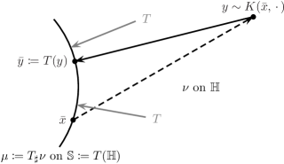
Figure 3.1: Illustration of the steps for drawing states using the naïve reprojection kernel $\bar{K}$ in (3.6) for $\mathbb{X}=\mathbb{H}$, $\mathbb{Y}=\mathbb{S}$, and $T=\Pi^{\mathbb{S}}$ in (3.1). Starting from $\bar{x}$, an intermediate state $y\in\mathbb{H}$ is drawn from the $\nu$-reversible transition kernel $K(\bar{x},\hbox to5.71527pt{\hss$\cdot$\hss})$ on $\mathbb{H}$. The next state drawn from the naïve reprojection kernel $\bar{K}(\bar{x},\hbox to5.71527pt{\hss$\cdot$\hss})$ is then $\bar{y}\coloneqq T(y)=\Pi^{\mathbb{S}}(y)$. Solid arrows indicate deterministic maps, whereas dashed arrows indicate randomised maps, i.e. draws from transition kernels.

Unlike the projection approach described earlier, this method yields a Markov chain. However, as numerical experiments show, the naïve reprojection kernel $\bar{K}$ does not have $\mu$ as its stationary distribution, even if $K$ is $\nu$-invariant or $\nu$-reversible. To see why, recall that $\mu=T_{\sharp}\nu$. Hence, $\bar{K}$ is $\mu$-invariant if and only if

$$\int_{\mathbb{Y}}\bar{K}(\bar{x},A)\,\mu(\mathrm{d}\bar{x}) =\int_{\mathbb{Y}}K(\bar{x},T^{-1}(A))\,\mu(\mathrm{d}\bar{x})=\int_{\mathbb{X}}K(T(x),T^{-1}(A))\,\nu(\mathrm{d}x)=\nu(T^{-1}(A))$$

for all $A\in\mathcal{B}(\mathbb{Y})$. If $K$ is $\nu$-invariant, then by definition $\nu(T^{-1}(A))=\int_{\mathbb{X}}K(x,T^{-1}(A))\,\nu(\mathrm{d}x)$. This yields the following necessary and sufficient condition for the $\mu$-invariance of $\bar{K}$:

$$\int_{\mathbb{X}}K(x,T^{-1}(A))\,\nu(\mathrm{d}x)=\int_{\mathbb{X}}K(T(x),T^{-1}(A))\,\nu(\mathrm{d}x),\qquad\forall A\in\mathcal{B}(\mathbb{Y}).$$

Based upon numerical experiments, we argue that this condition is not necessarily satisfied in the setting where $\mathbb{X}=\mathbb{H}$, $\mathbb{Y}=\mathbb{S}$, and $T=\Pi^{\mathbb{S}}$. Let $\mathbb{H}=\mathbb{R}^{3}$, $\nu=\mathrm{N}(0,C)$ with covariance matrix $C\in\mathbb{R}^{3\times 3}$, and consider the $\nu$-reversible pCN proposal kernel

$$K(x)=\mathrm{N}\Bigl{(}\sqrt{1-s^{2}}x,s^{2}C\Bigr{)},\quad\text{ with }\quad s=0.7\text{ and }\ C=\begin{pmatrix}1.25&0.33&-1.62\\ 0.33&0.42&-0.09\\ -1.62&-0.09&2.85\end{pmatrix}.$$

We now estimate and compare the probability density function of the marginals of $\mu=\Pi^{\mathbb{S}}_{\sharp}\nu$ and $\mu\bar{K}$ by kernel density estimation based on $10^{6}$ independent samples of $\mu$ and $\mu\bar{K}$, respectively. The results are displayed in Figure 3.2. The important observation is that the marginals of $\mu$ (dashed yellow line) and $\mu\bar{K}$ (dotted blue line) differ. Hence, $\bar{K}$ is not $\mu$-invariant in this case. Note that the marginals of $\mu$ (dashed yellow line) coincide with the marginals of $\mu(\Pi^{\mathbb{S}}_{\sharp}K)$ (solid red line), where $\Pi^{\mathbb{S}}_{\sharp}K$ is the $\mu$-reversible transition kernel of the reprojected Markov chain using the push-forward transition kernel $T_{\sharp}K$ in (3.7).

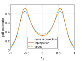
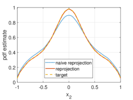
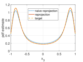
Figure 3.2: Comparison of marginals of $\mu=\Pi^{\mathbb{S}}_{\sharp}\nu$ (target), $\mu\bar{K}$ (naïve reprojection) with $\bar{K}$ as in (3.6), and $\mu(\Pi^{\mathbb{S}}_{\sharp}K)$ (reprojection) with $\Pi^{\mathbb{S}}_{\sharp}K$ as in (3.9) with pCN-kernel $K$ and $T=\Pi^{\mathbb{S}}$.

3.2 The reprojection method

We present now a simple method for defining a $\mu$-reversible Markov chain $(\bar{X}_{n})_{n\in\mathbb{N}}$ on $\mathbb{S}$, by using a $\nu$-reversible transition kernel $K$ on $\mathbb{H}$. The method employs the concept of push-forward transition kernels which we explain for the general setting of Polish spaces $\mathbb{X},\mathbb{Y}$ connected via a measurable mapping $T\colon\mathbb{X}\to\mathbb{Y}$. For more details of this approach we refer to (Rudolf and Sprungk, 2022). For the particular algorithms that we consider later, we focus on the specific case of $\mathbb{Y}=\mathbb{S}$, $\mathbb{X}=\mathbb{H}$, and $T$ the radial projection map $T=\Pi^{\mathbb{S}}$ given in (3.1).

Given a $\nu$-invariant transition kernel $K$ on $\mathbb{X}$ and a measurable map $T\colon\mathbb{X}\to\mathbb{Y}$, we define the push-forward transition kernel $T_{\sharp}K$ on $\mathbb{Y}$ as follows:

$$T_{\sharp}K(\bar{x},A)\coloneqq\mathbb{E}\left[K(X,T^{-1}(A))\mid T(X)=\bar{x}\right],\qquad X\sim\nu,$$ (3.7)

where $\bar{x}\in\mathbb{Y}$ and $A\in\mathcal{B}(\mathbb{Y})$. If $T$ is bijective, then

$$T_{\sharp}K(\bar{x},A)=K(T^{-1}(\bar{x}),T^{-1}(A)).$$

In the following, we also use the shorter notation $\bar{K}=T_{\sharp}K$. Below, we summarise some important properties of push-forward transition kernels that are inherited from the original transition kernel.

Lemma 3.2 (Rudolf and Sprungk, 2022).

Let $\mathbb{X}$ and $\mathbb{Y}$ be Polish spaces, $T\colon\mathbb{X}\to\mathbb{Y}$ be a measurable mapping, $K$ be a $\nu$-invariant transition kernel on $\mathbb{X}$, and $\mu\coloneqq T_{\sharp}\nu$.

1. If $K$ is reversible with respect to $\nu$, then $T_{\sharp}K$ is reversible with respect to $\mu$.

2. If $K$ has an $L^{2}_{\nu}$-spectral gap, then $T_{\sharp}K$ has an $L^{2}_{\mu}$-spectral gap and

   $$\operatorname{gap}_{\mu}(T_{\sharp}K)\geqslant\operatorname{gap}_{\nu}(K).$$

3. If $K$ is an MH kernel with proposal kernel $Q\colon\mathbb{X}\times\mathcal{B}(\mathbb{X})\to[0,1]$ and acceptance probability $\alpha\colon\mathbb{X}\times\mathbb{X}\to[0,1]$ such that

   $$\alpha(x,y)=\bar{\alpha}(T(x),T(y))\qquad\forall x,y\in\mathbb{X}$$

   for a measurable $\bar{\alpha}\colon\mathbb{Y}\times\mathbb{Y}\to[0,1]$, then $T_{\sharp}K$ is an MH kernel with acceptance probability $\bar{\alpha}$ and proposal kernel $\bar{Q}$ given by

   $$\bar{Q}(\bar{x},A)\coloneqq\int_{\mathbb{X}}Q(x,T^{-1}(A))\,\nu_{|T}(\bar{x},\mathrm{d}x),\qquad\forall\bar{x}\in\mathbb{Y},\ A\in\mathcal{B}(\mathbb{Y}),$$

   where $\nu_{|T}(\bar{x},\hbox to5.71527pt{\hss$\cdot$\hss})$ denotes the regular conditional distribution of $X\sim\nu$ given $T(X)=\bar{x}$.

See Section B.1 for the definition of the spectral gap of a transition kernel $K$.

The last item in the above lemma also shows that one can simulate push-forward transition kernels by exploiting the regular conditional distribution $\nu_{\mid T}\colon\mathbb{Y}\times\mathcal{B}(\mathbb{X})\to[0,1]$ of $X\sim\nu$ given $T(X)=\bar{x}$. We recall that $\nu_{\mid T}$ possesses the properties of a transition kernel and satisfies

$$\nu_{|T}(T(X),A)=\mathbb{P}\left(X\in A\ \middle|\ T(X)\right)\qquad\mathbb{P}\text{-almost surely},$$ (3.8)

for any $A\in\mathcal{B}(\mathbb{X})$. Given this regular conditional distribution, the disintegration theorem yields the representation

$$T_{\sharp}K(\bar{x},A)=\int_{\mathbb{X}}K(x,T^{-1}(A))\,\nu_{|T}(\bar{x},\mathrm{d}x),$$ (3.9)

for general transition kernels $K$. Thus, the push-forward transition kernel $T_{\sharp}K$ can be realised by the following mechanism.

Transition Mechanism 3.3.

Given the current state $\bar{x}\in\mathbb{Y}$ one obtains the next state $\bar{y}\in\mathbb{Y}$ as follows:

1. Draw $X\sim\nu_{|T}(\bar{x},\hbox to5.71527pt{\hss$\cdot$\hss})$ and call the realisation $x\in\mathbb{X}$;

2. Draw $Y\sim K(x,\hbox to5.71527pt{\hss$\cdot$\hss})$, call the realisation $y\in\mathbb{X}$ and return $\bar{y}\coloneqq T(y)\in\mathbb{Y}$.

We now consider the specific case of $\mathbb{X}=\mathbb{H}$ being a Hilbert space, $\mathbb{Y}=\mathbb{S}$ its unit sphere and $T=\Pi^{\mathbb{S}}$ being the radial projection defined in (3.1). In order to obtain a $\mu$-reversible Markov chain on $\mathbb{S}$, we can consider the push-forward transition kernels $\bar{K}=T_{\sharp}K$ of $\nu$-reversible transition kernels $K$ on the ambient Hilbert space $\mathbb{H}$ — such as the pCN-MH kernel or the ESS kernel — provided that we can also simulate the regular conditional distribution $\nu_{\mid T}$ for the lifted target $\nu$ in (3.4). The resulting algorithm is illustrated in Figure 3.3. In particular, by going randomly from $\bar{x}$ to $x$ in the ambient space, performing a transition from $x$ to $y$ by using $K$, and then by “reprojecting” deterministically from $y$ to $\bar{y}=\Pi^{\mathbb{S}}(y)$, we end up on the sphere $\mathbb{S}$. Since this is performed at each iteration of the Markov chain, we name this the reprojection method.

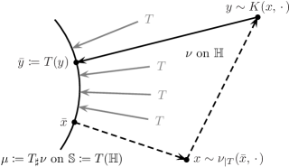
Figure 3.3: Illustration of the steps in the reprojection method from Section 3.2. The reprojection method defines a $\mu$-reversible transition kernel on $\mathbb{S}$ in terms of a $\nu$-reversible transition kernel $K$ on the ambient space $\mathbb{H}$, where $\mathbb{S}\coloneqq T(\mathbb{H})$, $\mu\coloneqq T_{\sharp}\nu$, $\nu_{|T}(\bar{x},\hbox to5.71527pt{\hss$\cdot$\hss})$ is the regular conditional distribution of $X\sim\nu$ given $T(X)=\bar{x}$, and $T=\Pi^{\mathbb{S}}$. Solid arrows indicate deterministic maps, whereas dashed arrows indicate randomised maps, i.e. draws from transition kernels.

Next, we derive the regular conditional distribution $\nu_{|\Pi^{\mathbb{S}}}$ for Gaussian measures $\nu=\mathrm{N}(0,C)$ on $\mathbb{H}=\mathbb{R}^{d}$, and state the resulting reprojected pCN-MH algorithm as well as the reprojected ESS algorithm.

Simulating the conditional distribution $\nu_{|\Pi^{\mathbb{S}}}$.

We first prove a proposition about the regular conditional distributions $\nu_{|T}$ in the more general setting of Polish spaces $\mathbb{X},\mathbb{Y}$. We then apply this proposition to derive an explicit description for $\nu_{|\Pi^{\mathbb{S}}}$. One can modify this procedure for manifolds in Hilbert spaces that are more general than the unit sphere $\mathbb{S}$, e.g. manifolds that can be described by a measurable mapping $T\colon\mathbb{H}\to\mathbb{H}$, by replacing $\Pi^{\mathbb{S}}$ with $T$.

Proposition 3.4.

Let $\mathbb{X}$ and $\mathbb{Y}$ be Polish spaces equipped with a measurable mapping $T\colon\mathbb{X}\to\mathbb{Y}$ and $\nu_{0}\in\mathcal{P}(\mathbb{X})$. Let $\bar{\Phi}\colon\mathbb{Y}\to\mathbb{R}$ be measurable with $Z\coloneqq\int_{\mathbb{Y}}\exp(-\bar{\Phi}(T(x)))\,\nu_{0}(\mathrm{d}x)<\infty$, define $\Phi\colon\mathbb{X}\to\mathbb{R}$ by $\Phi(x)\coloneqq\bar{\Phi}(T(x))$ for $x\in\mathbb{X}$, and let $\nu\in\mathcal{P}(\mathbb{X})$ be given by

$$\frac{\mathrm{d}\nu}{\mathrm{d}\nu_{0}}(x)=\frac{1}{Z}\exp(-\Phi(x)),\quad\nu_{0}\text{-a.e.\ }x\in\mathbb{X}.$$

Furthermore, let $\nu_{0|T}$ be the regular conditional distribution of $X_{0}\sim\nu_{0}$ given $T(X_{0})$, and let $\nu_{|T}$ be the regular conditional distribution of $X\sim\nu$ given $T(X)$. Then

$$\nu_{|T}(T(x),\hbox to5.71527pt{\hss$\cdot$\hss})=\nu_{0|T}(T(x),\hbox to5.71527pt{\hss$\cdot$\hss})$$

for $\nu_{0}$-a.e. $x\in\mathbb{X}$.

The hypotheses of the proposition differ from the hypotheses of Proposition 3.1 only in the additional assumption that $\mathbb{X}$ and $\mathbb{Y}$ are Polish spaces. This assumption ensures that we may apply the disintegration theorem to obtain regular conditional distributions. We can weaken the assumption by requiring that $\mathbb{X}$ and $\mathbb{Y}$ be merely Radon spaces.

Proof of Proposition 3.4. The regular conditional distribution $\nu_{0|T}\colon\mathbb{Y}\times\mathcal{B}(\mathbb{X})\to[0,1]$ of $X_{0}$ given $T(X_{0})$ is defined as a Markov kernel satisfying for every $A\in\mathcal{B}(\mathbb{X})$ and $B\in\mathcal{B}(\mathbb{Y})$,

$$\mathbb{P}(X_{0}\in A,\ T(X_{0})\in B)=\int_{B}\nu_{0|T}(y,A)\,T_{\sharp}\nu_{0}(\mathrm{d}y)=\int_{T^{-1}(B)}\nu_{0|T}(T(x),A)\,\nu_{0}(\mathrm{d}x).$$

Moreover, given the regular conditional distribution $\nu_{0|T}$ we can express the conditional expectation of $g(X_{0})$ given $T(X_{0})$ for any measurable $g\colon\mathbb{X}\to\mathbb{R}$ as

$$\mathbb{E}\left[g(X_{0})\mid T(X_{0})\right]=\int_{\mathbb{X}}g(x)\ \nu_{0|T}(T(X_{0}),\mathrm{d}x)\qquad\mathbb{P}\text{-almost surely}.$$ (3.10)

We ask now for the regular conditional distribution $\nu_{|T}$ of $X\sim\nu$ given $T(X)$. Analogously, this is a Markov kernel $\nu_{|T}\colon\mathbb{Y}\times\mathcal{B}(\mathbb{X})\to[0,1]$ satisfying

$$\mathbb{P}(X\in A,\ T(X)\in B)=\int_{B}\nu_{|T}(y,A)\,T_{\sharp}\nu(\mathrm{d}y)=\int_{T^{-1}(B)}\nu_{|T}(T(x),A)\,\nu(\mathrm{d}x)$$

for every $A\in\mathcal{B}(\mathbb{X})$ and $B\in\mathcal{B}(\mathbb{Y})$. Since $\mathbb{P}(X\in A,\ T(X)\in B)=\nu(A\cap T^{-1}(B))$, the statement follows if

$$\nu(A\cap T^{-1}(B))=\int_{T^{-1}(B)}\nu_{0|T}(T(x),A)\,\nu(\mathrm{d}x)\qquad\forall A\in\mathcal{B}(\mathbb{X})\ \forall B\in\mathcal{B}(\mathbb{Y}),$$ (3.11)

because $\nu_{0|T}$ is then a valid regular conditional distribution of $X\sim\nu$ given $T(X)$. For $A\in\mathcal{B}(\mathbb{X})$ and $B\in\mathcal{B}(\mathbb{Y})$,

$$\nu(A\cap T^{-1}(B)) =\int_{\mathbb{X}}\mathds{1}_{A}(x)\ \mathds{1}_{B}(T(x))\ \frac{1}{Z}\mathrm{e}^{-\Phi(x)}\ \nu_{0}(\mathrm{d}x)=\mathbb{E}\left[\frac{1}{Z}\mathrm{e}^{-\Phi(X_{0})}\ \mathds{1}_{A}(X_{0})\ \mathds{1}_{B}(T(X_{0}))\right],$$

where $X_{0}\sim\nu_{0}$. Using the law of total expectation and the hypothesis that $\Phi(x)=\bar{\Phi}(T(x))$ for every $x\in\mathbb{X}$, we obtain

$$\nu(A\cap T^{-1}(B)) =\mathbb{E}\left[\mathbb{E}\left[\frac{1}{Z}\mathrm{e}^{-\Phi(X_{0})}\ \mathds{1}_{A}(X_{0})\ \mathds{1}_{B}(T(X_{0}))\,\Big{|}\,T(X_{0})\right]\right]$$

$$=\mathbb{E}\left[\frac{1}{Z}\mathrm{e}^{-\Phi(X_{0})}\ \mathds{1}_{B}(T(X_{0}))\ \mathbb{E}\left[\mathds{1}_{A}(X_{0})\mid T(X_{0})\right]\right].$$

Applying now (3.10) to $g(x)=\mathds{1}_{A}(x)$ yields $\mathbb{E}\left[\mathds{1}_{A}(X_{0})\mid T(X_{0})\right]=\nu_{0|T}(T(X_{0}),A)$ and, thus,

$$\nu(A\cap T^{-1}(B)) =\mathbb{E}\left[\frac{1}{Z}\mathrm{e}^{-\Phi(X_{0})}\ \mathds{1}_{B}(T(X_{0}))\ \nu_{0|T}(T(X_{0}),A)\right]$$

$$=\int_{T^{-1}(B)}\frac{1}{Z}\mathrm{e}^{-\Phi(x)}\ \nu_{0|T}(T(x),A)\ \nu_{0}(\mathrm{d}x)$$

$$=\int_{T^{-1}(B)}\nu_{0|T}(T(X_{0}),A)\ \nu(\mathrm{d}x)$$

which shows (3.11). $\blacksquare$

We now turn to the setting of a finite dimensional sphere, where $\mathbb{X}=\mathbb{R}^{d}$, $\mathbb{Y}=\mathbb{S}^{d-1}$, and $T=\Pi^{\mathbb{S}}$. In order to implement the reprojection method, it suffices by Proposition 3.4 to simulate the regular conditional distribution of $X_{0}\sim\mathrm{N}(0,C)$ given $\Pi^{\mathbb{S}}(X_{0})=\bar{x}$. In the following result $\mathrm{Gam}(a,b)$ denotes the Gamma distribution with shape parameter $a>0$ and inverse scale parameter $b>0$.

Proposition 3.5.

Let $\nu_{0}=\mathrm{N}(0,C)$ be given on $\mathbb{R}^{d}$ and let $\nu_{0\mid\Pi^{\mathbb{S}}}(\bar{x},\hbox to5.71527pt{\hss$\cdot$\hss})$ denote the conditional distribution of $X_{0}\sim\nu_{0}$ given $\Pi^{\mathbb{S}}(X_{0})=\bar{x}$. Then, for a non-negative real-valued random variable $R$ satisfying $R^{2}\sim\mathrm{Gam}\left(\frac{d}{2},\frac{1}{2}\bar{x}^{\top}C^{-1}\bar{x}\right)$,

$$R\bar{x}\sim\nu_{0\mid\Pi^{\mathbb{S}}}(\bar{x},\hbox to5.71527pt{\hss$\cdot$\hss}).$$

Proof. We can write $X_{0}\sim\nu=\mathrm{N}(0,C)$ as $X_{0}=R\bar{X}_{0}$, $\bar{X}_{0}\coloneqq\Pi^{\mathbb{S}}(X_{0})$, $R\coloneqq\|X_{0}\|$. Thus, the condition of $\Pi^{\mathbb{S}}(X_{0})=\bar{x}$ yields the following conditional density of $R$:

$$f_{R|\Pi^{\mathbb{S}}(X_{0})=\bar{x}}(r)\ \propto\ r^{d-1}\exp\left(-\frac{1}{2}(\bar{x}^{\top}C^{-1}\bar{x})r^{2}\right)=r^{d-1}\left(\exp\left(-\frac{1}{2}\bar{x}^{\top}C^{-1}\bar{x}\right)\right)^{r^{2}}.$$

By the change of variables $r\mapsto r^{2}\eqqcolon r_{2}$ we obtain the following probability density for $R^{2}$ given $\Pi^{\mathbb{S}}(X_{0})=\bar{x}$:

$$f_{R^{2}|\Pi^{\mathbb{S}}(X_{0})=\bar{x}}(r_{2})\ \propto\ \frac{r_{2}^{(d-1)/2}}{2r_{2}^{1/2}}\left(\mathrm{e}^{-\frac{1}{2}\bar{x}^{\top}C^{-1}\bar{x}}\right)^{r_{2}}\ \propto\ r_{2}^{d/2-1}\mathrm{e}^{-\left(\frac{1}{2}\bar{x}^{\top}C^{-1}\bar{x}\right){r_{2}}}.$$

Thus, $R^{2}$ conditioned on $\Pi^{\mathbb{S}}(X_{0})=\bar{x}$ follows the $\mathrm{Gam}(\frac{d}{2},\tfrac{1}{2}\bar{x}^{\top}C^{-1}\bar{x})$, as desired. $\blacksquare$

Resulting algorithms

We now provide two explicit algorithms for approximate sampling of target measures $\mu$ on $\mathbb{S}^{d-1}$ as given in (3.2). Algorithms 4 and 5 result from applying the push-forward transition kernel approach to the pCN-MH algorithm and the ESS algorithm on $\mathbb{H}$, respectively. The pCN-MH algorithm and the ESS algorithm on $\mathbb{H}$ were stated in Algorithms 1 and 2.

Algorithm 4 Reprojected pCN-MH algorithm on $\mathbb{S}^{d-1}$

1:  Given: ACG prior $\mu_{0}=\mathrm{ACG}(C)$ and target $\mu$ as in (3.2)

2:  Initial: step size $s\in(0,1]$ and state $\bar{x}_{0}\in\mathbb{S}^{d-1}$

3:  for $k\in\mathbb{N}_{0}$ do

4:     Draw a sample $r_{k}^{2}$ of $\mathrm{Gam}\left(d/2,\frac{1}{2}\bar{x}_{k}^{\top}C^{-1}\bar{x}_{k}\right)$ and set $x_{k}=r_{k}\bar{x}_{k}$

5:     Draw a sample $w_{k}$ of $\mathrm{N}(0,C)$ and set $y_{k+1}\coloneqq\sqrt{1-s^{2}}x_{k}+sw_{k}$

6:     Set $\bar{y}_{k+1}\coloneqq y_{k+1}/\|y_{k+1}\|$

7:     Compute $a\coloneqq\min\{1,\exp\left(\bar{\Phi}(\bar{x}_{k})-\bar{\Phi}(\bar{y}_{k+1})\right)\}$

8:     Draw a sample $u$ of $\mathrm{U}[0,1]$

9:     if $u\leqslant a$ then

10:        Set $\bar{x}_{k+1}=\bar{y}_{k+1}$

11:     else

12:        Set $\bar{x}_{k+1}=\bar{x}_{k}$

13:     end if

14:  end for

Algorithm 5 Reprojected ESS algorithm on $\mathbb{S}^{d-1}$

1:  Given: ACG prior $\mu_{0}=\mathrm{ACG}(C)$ and target $\mu$ as in (3.2)

2:  Initial: state $\bar{x}_{0}\in\mathbb{S}^{d-1}$

3:  for $k\in\mathbb{N}_{0}$ do

4:     Draw a sample $t\sim\mathrm{U}[0,\exp(-\bar{\Phi}(\bar{x}_{k}))]$

5:     Draw a sample $r_{k}^{2}$ of $\mathrm{Gam}\left(d/2,\frac{1}{2}\bar{x}_{k}^{\top}C^{-1}\bar{x}_{k}\right)$ and set $x_{k}=r_{k}\bar{x}_{k}$

6:     Set $x_{k+1}=\text{shrink-ellipse}(x_{k},t)$   (see Algorithm 3)

7:     Set $\bar{x}_{k+1}=x_{k+1}/\|x_{k+1}\|$

8:  end for

According to Lemma 3.2(c), Algorithm 4 yields an MH algorithm on $\mathbb{S}^{d-1}$. Its acceptance probability is simply $\bar{\alpha}(\bar{x},\bar{y})=\min\{1,\exp\left(\bar{\Phi}(\bar{y})-\bar{\Phi}(\bar{x})\right)\}$, for $\bar{x},\bar{y}\in\mathbb{S}^{d-1}$, and its proposal kernel $\bar{Q}\colon\mathbb{S}^{d-1}\times\mathcal{B}(\mathbb{S}^{d-1})\to[0,1]$ admits a proposal density $\bar{q}\colon\mathbb{S}^{d-1}\times\mathbb{S}^{d-1}\to(0,\infty)$ with respect to the Hausdorff measure on $\mathbb{S}^{d-1}$ given by

$$\bar{q}(\bar{x},\bar{y})=\int_{0}^{\infty}\int_{0}^{\infty}q(r\bar{x},r^{\prime}\bar{y})\ f_{\bar{x}}(r)\,(r^{\prime})^{d-1}\,\mathrm{d}r\,\mathrm{d}r^{\prime}>0,\qquad\bar{x},\bar{y}\in\mathbb{S}^{d-1},$$ (3.12)

where $q$ denotes the proposal density of the pCN proposal kernel $Q(x,\hbox to5.71527pt{\hss$\cdot$\hss})=\mathrm{N}(\sqrt{1-s^{2}}x,s^{2}C)$, $x\in\mathbb{R}^{d}$, and $f_{\bar{x}}(r)$ denotes the conditional density of $R=\|X\|$ for $X\sim\mathrm{N}(0,C)$ given $\Pi^{\mathbb{S}}(X)=\bar{x}$. According to the proof of Proposition 3.5, the density $f_{\bar{x}}(r)$ takes the form

$$f_{\bar{x}}(r)\coloneqq\frac{1}{c_{\bar{x}}}r^{d-1}\exp\left(-\frac{r^{2}}{2}\bar{x}^{\top}C^{-1}\bar{x}\right),\qquad c_{\bar{x}}\coloneqq\int_{0}^{\infty}r^{d-1}\exp\left(-\frac{r^{2}}{2}\bar{x}^{\top}C^{-1}\bar{x}\right)\mathrm{d}r.$$ (3.13)

Remark 3.6.

Due to the generality of the pushforward Markov kernel approach, it is also possible to combine the reprojection methodology that we proposed with other common MH algorithms, such as the dimension-independent Hamiltonian Monte Carlo (HMC) algorithm of Beskos et al. (2011). However, an extensive investigation of a reprojected HMC algorithm that shows advantages and disadvantages, e.g. in comparison to the work of Lan et al. (2014), is beyond the scope of this paper.

3.3 Uniform and geometric ergodicity

We investigate the exponential convergence behaviour of the transition kernels that correspond to the Markov chains that are realised either by Algorithm 4 or Algorithm 5. Since the underlying state space $\mathbb{S}^{d-1}$ is compact, we aim for uniform ergodicity. The associated transition kernel $\bar{K}\colon\mathbb{S}^{d-1}\times\mathcal{B}(\mathbb{S}^{d-1})\to[0,1]$ is said to be uniformly ergodic, if there are $\kappa\in[0,1)$ and $c<\infty$ such that

$$\|\bar{K}^{n}(\bar{x})-\mu\|_{\mathrm{TV}}\leqslant c\,\kappa^{n}\qquad\forall\bar{x}\in\mathbb{S}^{d-1}.$$ (3.14)

It is well known (e.g. Meyn and Tweedie, 2009, Theorem 16.0.2) that uniform ergodicity of a Markov chain is equivalent to the smallness of the whole state space. A set $B\in\mathcal{B}(\mathbb{S}^{d-1})$ is called small with respect to a transition kernel $\bar{K}$ if there exists some $m\in\mathbb{N}$ and a nonzero measure $\phi$ on $(\mathbb{S}^{d-1},\mathcal{B}(\mathbb{S}^{d-1}))$ such that

$$\bar{K}^{m}(\bar{x},A)\geqslant\phi(A)\qquad\forall A\in\mathcal{B}(\mathbb{S}^{d-1}),\ \bar{x}\in B.$$ (3.15)

In particular, if (3.15) holds for $B=\mathbb{S}^{d-1}$, then (Meyn and Tweedie, 2009, Theorem 16.2.4) yields that

$$\|\bar{K}^{n}(\bar{x})-\mu\|_{\mathrm{TV}}\leqslant(1-\phi(\mathbb{S}^{d-1}))^{n/m-1}$$ (3.16)

By exploiting the particular structure (3.9) of push-forward transition kernels, we obtain the following result.

Theorem 3.7.

Let $\bar{\Phi}\colon\mathbb{S}^{d-1}\to\mathbb{R}$ be uniformly bounded. Then the transition kernels corresponding to the Markov chains realised by Algorithms 4 and 5 are uniformly ergodic.

Proof. The idea of the proof is to show that, in both cases, the state space is small.

We first consider the reprojected pCN-MH kernel $\bar{K}$. The boundedness of $\bar{\Phi}$, i.e. $\underline{c}\leqslant\bar{\Phi}(\bar{x})\leqslant\overline{c}$, yields the following lower bound on the acceptance probability:

$$\bar{\alpha}(\bar{x},\bar{y})=\min\left\{1,\exp\left(\bar{\Phi}(\bar{y})-\bar{\Phi}(\bar{x})\right)\right\}\geqslant\exp(\underline{c}-\overline{c})>0.$$

Hence, by the corresponding MH form of the reprojected pCN-MH kernel $\bar{K}$ stated in Lemma 3.2, for any $A\in\mathcal{B}(\mathbb{S}^{d-1})$ and any $\bar{x}\in\mathbb{S}^{d-1}$,

$$\bar{K}(\bar{x},A)\geqslant\int_{A}\bar{\alpha}(\bar{x},\bar{y})\ \bar{Q}(\bar{x},\mathrm{d}\bar{y})\geqslant\exp(\underline{c}-\overline{c})\ \bar{Q}(\bar{x},A).$$

Recall that $\bar{Q}$ possesses the density $\bar{q}$ given in (3.12). Note that $\bar{x}\mapsto\bar{x}^{\top}C^{-1}\bar{x}$ is bounded on $\mathbb{S}^{d-1}$, such that there exists for every $r>0$ a lower bound $\underline{f}(r)>0$ satisfying $f_{\bar{x}}(r)\geqslant\underline{f}(r)>0$ for every $\bar{x}\in\mathbb{S}^{d-1}$. Moreover, the density $q(\hbox to5.71527pt{\hss$\cdot$\hss},y)$ of the pCN proposal kernel $Q(x,\hbox to5.71527pt{\hss$\cdot$\hss})=\mathrm{N}(\sqrt{1-s^{2}}x,s^{2}C)$ is continuous. Therefore, $q(x,y)$ is uniformly bounded away from zero for any $x,y\in\mathbb{R}^{d}$ with $\|x\|,\|y\|\leqslant 1$. Hence, there exists some $\epsilon>0$ such that, for every $\bar{x},\bar{y}\in\mathbb{S}^{d-1}$, $\bar{q}(\bar{x},\bar{y})$ in (3.12) satisfies $\bar{q}(\bar{x},\bar{y})\geqslant\epsilon$. This implies that $\bar{Q}(\bar{x},A)\geqslant\epsilon\mathcal{H}_{\mathbb{S}^{d-1}}(A)$, for the Hausdorff measure $\mathcal{H}_{\mathbb{S}^{d-1}}$ on $\mathbb{S}^{d-1}$. Thus, $\mathbb{S}^{d-1}$ is small with respect to $\bar{K}$ with $\phi(A)\coloneqq\epsilon\exp(\underline{c}-\overline{c})\mathcal{H}_{\mathbb{S}^{d-1}}(A)$.

Next, we consider the reprojected ESS kernel. Since $\Phi$ on $\mathbb{H}=\mathbb{R}^{d}$ is constructed from $\bar{\Phi}$ on $\mathbb{S}$ by (3.3), the boundedness of $\bar{\Phi}$ implies the boundedness of $\Phi$. Hence, any compact set $B\subset\mathbb{R}^{d}$ is small with respect to the ESS transition kernel $K$. The measure with respect to which the smallness property holds is $\phi=\epsilon_{B}\lambda_{B}$, where $\epsilon_{B}>0$ denotes a constant and $\lambda_{B}$ is the Lebesgue measure restricted to a compact set $B$ with positive $d$-dimensional Lebesgue measure; see (Natarovskii et al., 2021a, Lemma 3.4). We now use this fact in order to show the smallness of $\mathbb{S}^{d-1}$ with respect to the reprojected ESS transition kernel $\bar{K}$ for the measure $\phi=\epsilon\mathcal{H}_{\mathbb{S}^{d-1}}$ for appropriately chosen $\epsilon>0$, see below. To this end, we apply the representation (3.9) with $\mathbb{X}=\mathbb{R}^{d}$, $\mathbb{Y}=\mathbb{S}^{d-1}$ and $T=\Pi^{\mathbb{S}}$:

$$\bar{K}(\bar{x},A)=\int_{0}^{\infty}K(r\bar{x},T^{-1}(A))f_{\bar{x}}(r)\,\mathrm{d}r$$

with $f_{\bar{x}}$ as in (3.13). Again, since $\bar{x}\mapsto\bar{x}^{\top}C^{-1}\bar{x}$ is bounded on $\mathbb{S}^{d-1}$, there exists for every $r>0$ a lower bound $\underline{f}(r)>0$ such that, for every $\bar{x}\in\mathbb{S}^{d-1}$, $f_{\bar{x}}(r)\geqslant\underline{f}(r)>0$. Now fix $B\coloneqq B_{1}(0)=\{x\in\mathbb{R}^{d}\mid\|x\|\leqslant 1\}$ and note that $B$ is small with respect to $K$. Thus

$$\bar{K}(\bar{x},A) \geqslant\int_{0}^{1}K(r\bar{x},T^{-1}(A))\underline{f}(r)\,\mathrm{d}r\geqslant\epsilon_{B}\lambda_{B}(T^{-1}(A))\,\int_{0}^{1}\underline{f}(r)\,\mathrm{d}r=\epsilon\mathcal{H}_{\mathbb{S}^{d-1}}(A)$$

where $\epsilon\coloneqq\epsilon_{B}\int_{0}^{1}\underline{f}(r)\,\mathrm{d}r\,\int_{0}^{1}u^{d-1}\,\mathrm{d}u$, since $\lambda_{B}(T^{-1}(A))=\int_{A}\int_{0}^{1}u^{d-1}\mathrm{d}u\,\mathcal{H}_{\mathbb{S}^{d-1}}(\mathrm{d}\bar{x})$. $\blacksquare$

The boundedness assumption on $\bar{\Phi}$ in Theorem 3.7 is rather mild. It is satisfied if $\bar{\Phi}\colon\mathbb{S}^{d-1}\to\mathbb{R}$ is continuous. For example, in the Bayesian level set inversion and Bayesian density estimation problems considered in Section 4, the corresponding $\bar{\Phi}$ is bounded.

Theorem 3.7 yields uniform ergodicity in finite dimension. In the last paragraph of the proof of Theorem 3.7, we considered the measure $\phi\coloneqq\epsilon\exp(\underline{c}-\overline{c})\mathcal{H}_{\mathbb{S}^{d-1}}$ for the reprojected pCN-MH kernel $\bar{K}$ and the measure $\phi\coloneqq\epsilon\mathcal{H}_{\mathbb{S}^{d-1}}$ for the reprojected ESS kernel. Supposing that the pre-factors $\epsilon$ and $\epsilon\exp(\underline{c}-\overline{c})$ do not grow in $d$ and substituting these choices of $\phi$ in (3.16) we observe that the corresponding $\kappa=(1-\phi(\mathbb{S}^{d-1}))^{1/m}$ in (3.14), with $c=(1-\phi(\mathbb{S}^{d-1}))^{-1}$, converges exponentially quickly to 1 as $d\to\infty$. This is because the $(d-1)$-dimensional Hausdorff measure of $\mathbb{S}^{d-1}$ is given by $\tfrac{2\pi^{d/2}}{\Gamma(d/2)}$, where $\Gamma(\hbox to5.71527pt{\hss$\cdot$\hss})$ is the Gamma function, and because of the asymptotic behaviour of $\Gamma(\hbox to5.71527pt{\hss$\cdot$\hss})$.

In the subsequent paragraph, we present a dimension-independent convergence behaviour, but in the context of geometric ergodicity as in (B.5), and not in the context of uniform ergodicity as in (3.14).

Dimension-independent geometric ergodicity.

In order to study the geometric ergodicity of Markov chains generated by the reprojected pCN-MH and reprojected ESS algorithms, we can exploit Lemma 3.2. This lemma states that the spectral gaps of the reprojected transition kernels $\bar{K}$ of Algorithms 4 and 5 are at least as large as the spectral gaps of the transition kernels $K$ of Algorithms 1 and 2 respectively. In order to describe a dimension-independent spectral gap, we introduce the following notation: Given $\mu_{0}=\mathrm{ACG}(C)$ with non-degenerate, trace-class covariance operator $C\colon\mathbb{H}\to\mathbb{H}$ on an infinite-dimensional separable Hilbert space $\mathbb{H}$, let $\{e_{j}\mid j\in\mathbb{N}\}$ be a complete orthonormal system in $\mathbb{H}$ consisting of the eigenvectors of $C$. We now construct finite-dimensional approximations to the infinite-dimensional setting as follows: For $d\in\mathbb{N}$, let $\mu^{(d)}_{0}=\mathrm{ACG}(C_{d})$ denote the ACG measure on $\mathbb{S}^{d-1}$ resulting from the marginal of $\mathrm{N}(0,C)$ on $\operatorname*{span}\left\{e_{1},\ldots,e_{d}\right\}$ and consider the target measure $\mu^{(d)}$ on $\mathbb{S}^{d-1}$ given by

$$\frac{\mathrm{d}\mu^{(d)}}{\mathrm{d}\mu^{(d)}_{0}}(\bar{x})\propto\exp(-\bar{\Phi}(\bar{x})),\quad\bar{x}\in\mathbb{S}^{d-1}.$$ (3.17)

In order to apply $\bar{\Phi}$ to $\bar{x}\in\mathbb{S}^{d-1}$, we view $\mathbb{S}^{d-1}$ as the “equatorial” subsphere $\{\bar{x}_{1}e_{1}+\ldots+\bar{x}_{d}e_{d}\in\mathbb{H}\colon\bar{x}=(\bar{x}_{1},\ldots,\bar{x}_{d})\in\mathbb{S}^{d-1}\}$ of $\mathbb{S}\subset\mathbb{H}$. Let

$$\frac{\mathrm{d}\nu^{(d)}}{\mathrm{d}\nu^{(d)}_{0}}(x)\propto\exp(-\Phi(x)),\quad x\in\mathbb{R}^{d},$$ (3.18)

where $\nu^{(d)}_{0}=\mathrm{N}(0,C_{d})$ and $\Phi(x)\coloneqq\bar{\Phi}(\Pi^{\mathbb{S}}(x))$ for $x\in\mathbb{H}$, as in (3.3). In order to apply $\Phi$ to $x\in\mathbb{R}^{d}$, we view $\mathbb{R}^{d}$ as the subspace $\{x_{1}e_{1}+\ldots+x_{d}e_{d}\in\mathbb{H}\colon x=(x_{1},\ldots,x_{d})\in\mathbb{R}^{d}\}$ of $\mathbb{H}$.

For a reminder of the definition of $\operatorname{gap}_{\mu}(K)$ for a given measure $\mu$ and transition kernel $K$ we refer to (B.4). By Lemma 3.2 we obtain the following result.

Proposition 3.8.

Let $\mu^{(d)}$ and $\nu^{(d)}$ be as in (3.17) and (3.18) respectively. Let $K^{(d)}$ denote the pCN-MH transition kernel targeting $\nu^{(d)}$ using a step size $s\in(0,1]$ in the proposal. If there exists a $\beta>0$ such that

$$\inf_{d\in\mathbb{N}}\operatorname{gap}_{\nu^{(d)}}\left(K^{(d)}\right)\geqslant\beta$$ (3.19)

then the reprojected pCN-MH transition kernel $\bar{K}^{(d)}\coloneqq(\Pi^{\mathbb{S}})_{\sharp}K^{(d)}$ targeting $\mu^{(d)}$ on $\mathbb{S}^{d-1}$ satisfies

$$\inf_{d\in\mathbb{N}}\operatorname{gap}_{\mu^{(d)}}\left(\bar{K}^{(d)}\right)\geqslant\beta.$$ (3.20)

The same statement holds for the reprojected ESS transition kernel $\bar{K}^{(d)}\coloneqq(\Pi^{\mathbb{S}})_{\sharp}K^{(d)}$.

Dimension independence of the spectral gap of the ESS transition kernel has been demonstrated in the literature by numerical experiments (Natarovskii et al., 2021a). However, to the best of our knowledge, no theoretical proof is available. Therefore, we focus on the pCN-MH algorithm, for which (3.19) was shown by Hairer et al. (2014) under certain assumptions on $\Phi$. For convenience, we summarise their result:

Theorem 3.9.

Let $K^{(d)}$ denote the pCN-MH transition kernel targeting $\nu^{(d)}$ using the step size $s\in(0,1]$ in the proposal. Suppose the following conditions hold:

1. There exist some $R>0$ and $\underline{\alpha}\in\mathbb{R}$ such that, for all $x\in\mathbb{H}$ with $\|x\|>R$,

   $$\Phi(y)<\Phi(x)-\underline{\alpha}\qquad\text{for all $y\in\mathbb{H}$ with $\bigl{\|}y-\sqrt{1-s^{2}}x\bigr{\|}\leqslant\frac{1}{2}\bigl{(}1-\sqrt{1-s^{2}}\bigr{)}\|x\|$.}$$

2. The function $\mathrm{e}^{-\Phi}$ is integrable with respect to $\nu_{0}=\mathrm{N}(0,C)$.

3. For every $\gamma>0$ there exists some $C_{\gamma}<\infty$ such that

   $$|\Phi(x)-\Phi(y)|\leqslant C_{\gamma}\mathrm{e}^{\gamma r}\qquad\text{for all $x,y\in\mathbb{H}$ with $\|x\|,\|y\|\leqslant r$.}$$

Then there exists a $\beta>0$ such that (3.19) holds.

The conditions of Theorem 3.9 are satisfied for constant $\Phi$. Thus, the pCN-MH transition kernel exhibits a dimension-independent spectral gap when targeting the prior $\nu=\nu_{0}=\mathrm{N}(0,C)$. By means of results by Vollmer (2015) and Rudolf and Sprungk (2018), this can then be lifted to bounded perturbations of the prior measure, such as $\mu$ as in (3.3) for bounded $\bar{\Phi}$. This yields our final result.

Theorem 3.10.

Let $\bar{\Phi}\colon\mathbb{S}^{d-1}\to\mathbb{R}$ be uniformly bounded. Then the transition kernel corresponding to the Markov chain realised by Algorithm 4 has a dimension-independent spectral gap in the sense of (3.20).

Proof. Let $K^{(d)}$ denote the pCN-MH transition kernel in $\mathbb{R}^{d}$ for an arbitrary step size $s\in(0,1]$ and dimension $d\in\mathbb{N}$ with target $\nu^{(d)}$, and let $K_{0}^{(d)}$ denote the pCN-MH transition kernel that targets the prior $\nu_{0}^{(d)}$. Note that $K_{0}^{(d)}$ coincides with the corresponding proposal kernel. By Theorem 3.9 we know that there exists a $\beta>0$ such that

$$\inf_{d\in\mathbb{N}}\operatorname{gap}_{\nu_{0}^{(d)}}\left(K_{0}^{(d)}\right)\geqslant\beta.$$

By (Rudolf and Sprungk, 2018, Theorem 11) the transition operator $K^{(d)}$ is positive, and hence,

$$\operatorname{gap}_{\nu_{0}^{(d)}}\left(K_{0}^{(d)}\right)=1-\Lambda_{\nu_{0}^{(d)}}\left(K_{0}^{(d)}\right),\qquad\operatorname{gap}_{\nu^{(d)}}\left(K^{(d)}\right)=1-\Lambda_{\nu^{(d)}}\left(K^{(d)}\right),$$

where $\Lambda_{\mu}(K)$ denotes the supremum of the spectrum of the restriction of a $\mu$-invariant transition operator $K$ to $L^{2}_{0,\mu}$, where $L^{2}_{0,\mu}\coloneqq\{f\in L^{2}(\mu)\mid\int f(u)\mu(\mathrm{d}u)=0\}$, and $L^{2}(\mu)\coloneqq\{f:\mathbb{H}\to\mathbb{R}\mid\|f\|_{L^{2}_{\mu}}\coloneqq\int|f|^{2}\mu(\mathrm{d}u)<\infty\}$. In the reversible case, $\Lambda_{\mu}(K)=\sup_{f\in L^{2}_{0,\mu}}\langle Kf,f\rangle_{L^{2}_{\mu}}/\|f\|_{L^{2}_{\mu}}$. Now, if $\bar{\Phi}$ is bounded, then so is $\Phi$. A comparison result (Vollmer, 2015, Theorem 3.3) states that

$$1-\Lambda_{\nu^{(d)}}\left(K^{(d)}\right)\geqslant\exp\left(4\inf\bar{\Phi}-4\sup\bar{\Phi}\right)\left(1-\Lambda_{\nu_{0}^{(d)}}\left(K_{0}^{(d)}\right)\right).$$

Applying this comparison result yields

$$\inf_{d\in\mathbb{N}}\operatorname{gap}_{\nu^{(d)}}\left(K^{(d)}\right)\geqslant\exp\left(4\inf\bar{\Phi}-4\sup\bar{\Phi}\right)\beta\ >\ 0$$

which by Proposition 3.8 yields the statement. $\blacksquare$

4 Numerical illustrations

We now demonstrate the dimension-independent performance of the reprojected pCN-MH algorithm and the reprojected ESS algorithm on two applications. Section 4.1, rooted in inverse problems, treats an application to Bayesian binary classification or level set inversion. Section 4.2 has a more statistical flavour and considers an application to Bayesian density estimation. Readers whose main interest is in the second application may proceed directly to Section 4.2 but may wish to recall the definition (4.8) of the root mean square jump distance with respect to the Riemannian metric on the sphere. We will use these applications to illustrate the dimension-dependent performance of the geodesic random walk-MH algorithm of Mangoubi and Smith (2018) and the MH algorithm of Zappa et al. (2018).

4.1 Bayesian binary level set inversion

For the convenience of the reader, we give a self-contained description of (Bayesian) binary level set inversion, following the presentation of Iglesias et al. (2016). Readers who are interested in technical details concerning the random fields perspective of level set inversion may consult Appendix 2 of that paper. For simplicity, we focus on the single-phase Darcy flow model or groundwater flow problem on a bounded domain $D\subset\mathbb{R}^{k}$, $k=1,2,3$, with closure $\overline{D}$ and boundary $\partial D$. This problem is described by the elliptic PDE

$$-\nabla\cdot(\mathrm{e}^{u}\nabla p) =f\text{ in }D,$$ (4.1a)

$$p =\kappa\text{ on }\partial D,$$ (4.1b)

where $p$ denotes a fluid pressure field, $f$ describes sources and sinks, and $u$ is the log-permeability parameter. Let $\mathcal{U}\coloneqq L^{\infty}(D)$ and $\mathcal{V}\coloneqq\{\tilde{p}\in H^{1}(D)\mid\tilde{p}=\kappa\text{ on }\partial D\}$, where $H^{1}(D)$ is the Sobolev space of functions in $L^{2}(D)$ whose first-order weak derivatives have finite $L^{2}(D)$ norm. If $u\in\mathcal{U}$, then $\mathrm{e}^{u}\in L^{\infty}(D)$, and given a suitable boundary condition $\kappa$ and source term $f\in L^{2}(D)$, a unique weak solution $p\in\mathcal{V}$ of (4.1) exists. Denote the solution map that maps the log-permeability $u$ to the corresponding solution $p$ by $\Upsilon\colon\mathcal{U}\to\mathcal{V}$. Then $\Upsilon$ is locally Lipschitz continuous, e.g., (Bonito et al., 2017).

We assume now that the domain $D$ is divided into two disjoint regions $D_{0},D_{1}\subset D$, i.e. $\overline{D}=D_{0}\cup D_{1}$. The subdomains $D_{i}$ describe the location of different materials, e.g., background and abnormal material, with different constant log-permeabilities $u_{0},u_{1}\in\mathbb{R}$. In particular, in binary level set inversion we assume that $u$ takes the form

$$u(t)=u_{0}\mathds{1}_{D_{0}}(t)+u_{1}\mathds{1}_{D_{1}}(t),\qquad t\in D,$$ (4.2)

where $\mathds{1}_{D_{i}}$ denotes the indicator function of $D_{i}$ and where the values $u_{0},u_{1}$ are known a priori.

The goal is then to infer the location of $D_{1}$ and, hence, $D_{0}=\overline{D}\setminus D_{1}$ based on noisy observations of $p$, i.e.,

$$y=O\circ\Upsilon(u)+\eta,$$ (4.3)

where $O\colon\mathcal{V}\to\mathbb{R}^{J}$ denotes for some $J\in\mathbb{N}$ a bounded linear observation operator and $\eta$ describes observational noise. We assume that $\eta\sim\mathrm{N}(0,\Sigma)$ with known covariance $\Sigma\in\mathbb{R}^{J\times J}$.

In the level set approach we then introduce a so-called level set function $g\in\mathbb{S}(L^{2}(D))\cap C(\overline{D})$ as well as the level set map $\mathcal{L}\colon C(\overline{D})\to\mathcal{U}$ defined by

$$g\mapsto\mathcal{L}(g)\coloneqq u_{0}\mathds{1}_{D_{0}(g)}+u_{1}\mathds{1}_{D_{1}(g)},\qquad D_{1}(g)\coloneqq\{t\in D\mid g(t)\geqslant 0\},$$ (4.4)

and $D_{0}(g)=\{t\in D\mid g(t)<0\}$, respectively. We can formulate the level set inverse problem as the problem of inferring the data-generating level set function $g$, given the model that the observations $y=O\circ\Upsilon\circ\mathcal{L}(g)+\eta$ are generated by a unique $g\in\mathbb{S}(L^{2}(D))\cap C(\overline{D})$. We argue that the unit sphere in the function space $L^{2}(D)$ or $C(\overline{D})$ is an advantageous setting for the level set inverse problem: if we considered the problem in the ambient space $g\in C(\overline{D})$, then $g$ becomes non-identifiable, because $\mathcal{L}(\alpha g)=\mathcal{L}(g)$ for any $\alpha>0$. For computational convenience, below we choose to work with the unit sphere in the Hilbert space $L^{2}(D)$ instead of the unit sphere in the Banach space $C(\overline{D})\subset L^{2}(D)$.

For the Bayesian approach to level set inversion, we use a prior for the level set function $g$ in the form of a series expansion

$$g=g(\bar{X})=\sum_{i=1}^{\infty}\bar{X}_{i}\phi_{i}$$ (4.5)

where the $\phi_{i}\in C(\overline{D})$ are given and form an orthonormal system in $L^{2}(D)$, and the $\bar{X}_{i}$ are random coefficients such that $\bar{X}=(\bar{X}_{i})_{i\in\mathbb{N}}\in\mathbb{S}(\ell^{2})$ almost surely; see e.g. (Iglesias et al., 2016; Dunlop et al., 2017). Then we have $g(\bar{X})\in\mathbb{S}(L^{2}(D))$ almost surely. A common choice for the system $\{\phi_{i}\mid i\in\mathbb{N}\}$ are the eigenfunctions of a covariance operator $C\colon L^{2}(D)\to L^{2}(D)$ given by $C\phi(t)=\int_{D}c(s,t)\,\phi(s)\,\mathrm{d}s$ and a continuous covariance function $c\in C(\overline{D}\times\overline{D})$. The latter then yields $\phi_{i}\in C(\overline{D})$ for every $i\in\mathbb{N}$, and by Mercer’s theorem we have $g(\bar{X})\in C(\overline{D})$ almost surely. In summary, we obtain a reformulation of the original level set inverse problem, as the problem of inferring the sequence $\bar{x}\in\mathbb{S}(\ell^{2})$ that corresponds to the data-generating level set function $g(\bar{x})$, given the noisy data $y=O\circ\Upsilon\circ\mathcal{L}(g(\bar{x}))+\eta$. For the prior $\mu_{0}$ on $\mathbb{S}(\ell^{2})$ in (3.2) we consider the ACG measure $\mu_{0}=\mathrm{ACG}(\Lambda)$ where $\Lambda=\mathrm{diag}(\lambda_{i}\colon i\in\mathbb{N})$ involves the eigenvalues $(\lambda_{i})_{i\in\mathbb{N}}$ of the covariance operator $C$, i.e., $C\phi_{i}=\lambda_{i}\phi_{i}$. The associated distribution of $g(\bar{X})$, $\bar{X}\sim\mathrm{ACG}(\Lambda)$, on $\mathbb{S}(L^{2}(D))$ is then $\mathrm{ACG}(C)$.

Remark 4.1 (Boundedness of $\bar{\Phi}$).

Given that $\eta\sim\mathrm{N}(0,\Sigma)$, the negative log-likelihood $\bar{\Phi}$ for Bayesian level set inversion on $\mathbb{S}$ takes the form

$$\bar{\Phi}(\bar{x})\coloneqq\frac{1}{2}\left\|\Sigma^{-1/2}\left(y-O\circ\Upsilon\circ\mathcal{L}(g(\bar{x}))\right)\right\|^{2}.$$

Since the range of $\mathcal{L}$ is bounded in $L^{\infty}(D)$, i.e. $\|\mathcal{L}(g)\|_{L^{\infty}(D)}\leqslant\max_{i}|u_{i}|$, and since $\Upsilon$ and $O$ are locally Lipschitz continuous and bounded respectively, we obtain that also $\bar{\Phi}$ is bounded on $\mathbb{S}(\ell^{2})$. Thus, the setting of Bayesian level set inversion satisfies the assumptions of Theorems 3.7 and 3.10. In particular, for finite-dimensional approximations of the Bayesian level set inversion problem that are obtained by truncating the expansion (4.5) after $d$ terms, Algorithms 4, 5 and 7 yield uniformly ergodic Markov chains on $\mathbb{S}^{d-1}$ targeting the corresponding posterior $\mu^{(d)}$. Here, the corresponding posterior $\mu^{(d)}$ on $\mathbb{S}^{d-1}$ may be obtained according to (3.17) or (3.18).

Problem setting.

We consider the elliptic problem (4.1) on $D=[0,1]$ with Dirichlet boundary conditions $p(0)=0$ and $p(1)=2$. For $u$ we assume a form as in (4.2) based on a decomposition of $D$ into two subregions $D_{0},D_{1}$ with corresponding values $u_{0}=-2$ and $u_{1}=2$.

For the level set function $g$ such that $u=\mathcal{L}(g)$ we assume a series expansion (4.5) based on the eigensystem of the covariance function

$$c(s,t)=\left(1+\sqrt{3}\frac{|t-s|}{0.1}\right)\,\exp\left(-\sqrt{3}\frac{|t-s|}{0.1}\right),$$ (4.6)

i.e. a Whittle–Matérn covariance with variance $\sigma^{2}=1$, correlation length $\rho=0.1$ and smoothness $\nu=1.5$. For computational reasons we truncate the representation (4.5) after $d$ terms and then infer the $d$ coefficients $\bar{x}_{1},\ldots,\bar{x}_{d}$ given noisy observations of $p(0.2)$, $p(0.4)$, $p(0.6)$, and $p(0.8)$.

The assumed noise model is $\eta\sim\mathrm{N}(0,\Sigma)$ where $\Sigma=\mathrm{diag}(\sigma^{2}_{1},\ldots,\sigma^{2}_{4})$ and $\sigma^{2}_{i}=p^{\dagger}(0.2i)/10$ where $p^{\dagger}$ denotes the “true” solution resulting from the “true” coefficient vector $x^{\dagger}=(1,2,3,4,5,1,1,1,0,\ldots,0)$ in the Karhunen–Loève expansion (4.5) of $g^{\dagger}$. For an illustration of $g^{\dagger}$, $u^{\dagger}$ and $p^{\dagger}$, see Figure 4.1.

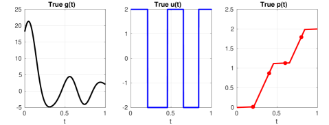
Figure 4.1: True $g^{\dagger}$, $u^{\dagger}$, $p^{\dagger}$, and true observations $o^{\dagger}=(p^{\dagger}(0.2),\ldots,p^{\dagger}(0.8))^{\top}$.

Given $\eta\sim\mathrm{N}(0,\Sigma)$ the negative log-likelihood for observed data $y\in\mathbb{R}^{4}$ is then

$$\Phi(x)\coloneqq\frac{1}{2}\sum_{j=1}^{4}\sigma_{j}^{-2}\left|y_{j}-F_{j}(x)\right|^{2},\qquad x\in\mathbb{R}^{d},$$

where $F_{j}$ denotes the forward mapping $x=(x_{i})_{i=1}^{d}\mapsto g\mapsto u\mapsto p\mapsto p(0.2j)$. As described in the previous subsection, $F_{j}(\alpha x)=F_{j}(x)$ for every $x\in\mathbb{R}^{d}$ and $\alpha>0$. Thus, $\Phi$ is invariant under the radial projection map $\Pi^{\mathbb{S}}$, i.e. $\Phi\circ\Pi^{\mathbb{S}}=\Phi$, and we can consider Bayesian level set inversion on the sphere $\mathbb{S}^{d-1}$ with corresponding prior

$$\mu_{0}=\mathrm{ACG}(\Lambda_{d}),\qquad\Lambda_{d}=\mathrm{diag}(\lambda_{1},\ldots,\lambda_{d}).$$

The posterior $\mu$ then takes the form (3.2) with $\bar{\Phi}(\bar{x})=\Phi(\bar{x})$. Figure 4.2 illustrates the prior, the likelihood and the resulting posterior for dimension $d=3$.

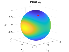
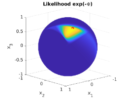
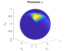
Figure 4.2: Prior, likelihood and posterior for dimension $d=3$; the red spot indicates the (projected) truth $\bar{x}^{\dagger}$.

Remark 4.2.

The eigenpairs $(\lambda_{j},\phi_{j})$ of the covariance operator $C$ associated to $c$ in (4.6) are computed numerically via a discretisation of $D$ and $C$ using a grid size of length $\delta t=10^{-3}$. The elliptic problem (4.1) is solved numerically using the same discretisation. Note that the solution $p$ of (4.1) on $D=[0,1]$ is given by $\Upsilon(u)(t)=p(t)=2S_{t}(\mathrm{e}^{-u})/S_{1}(\mathrm{e}^{-u})$ with $S_{t}(f)=\int_{0}^{t}f(s)\mathrm{d}s$. We evaluate $S_{t}$ using the trapezoidal rule on the given grid.

MCMC on the sphere.

We now apply the four MCMC algorithms described in Section 3 in order to sample approximately from the posterior $\mu$ in various dimensions $d$. In particular, we aim to compute the posterior expectation of the following quantity of interest:

$$f(\bar{x}) =\left(\int_{D}\exp(-u(t,\bar{x}))\,\mathrm{d}t\right)^{-1}$$ (4.7)

where $u(\hbox to5.71527pt{\hss$\cdot$\hss},\bar{x})=\mathcal{L}(g(\bar{x}))$. We may interpret $f(\bar{x})$ as the effective homogenised permeability field over the one-dimensional domain $D$; see e.g. (Alexanderian, 2015, Section 2).

First, we show in Figure 4.3 the thinned realisations $\bar{x}_{100k}$, $k=1,\ldots,100$ of the Markov chains generated by the reprojected pCN-MH algorithm, the geodesic random walk-MH algorithm based on (Mangoubi and Smith, 2018), and the MH algorithm of (Zappa et al., 2018) for $d=3$, subsampled every 100 steps.

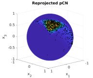
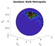
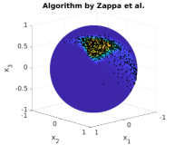
Figure 4.3: Thinned realisations $\bar{x}_{100k}$, $k=1,\ldots,100$ of the Markov chains generated by Algorithms 4, 6 and 7 (left, centre, and right, respectively) for $d=3$, subsampled every 100 steps.

All three MH algorithms were tuned to an average acceptance rate of roughly $23\%$. We ran the algorithms for another $10^{6}$ iterations after a burn-in period of $5\cdot 10^{4}$ iterations. All three runs yielded similar estimates for the posterior expectation of $f$. We provide the corresponding estimate plus/minus the half-length of an $95\%$ confidence interval based on asymptotic variance estimates via the empirical autocorrelation functions of $(f(\bar{x}_{k}))_{k}$:

reprojected pCN-MH: $$\quad 0.420\pm 1.299\cdot 10^{-3}$$

geodesic random walk-MH: $$\quad 0.419\pm 1.271\cdot 10^{-3}$$

MH by Zappa et al.: $$\quad 0.420\pm 1.478\cdot 10^{-3}.$$

All three estimates exhibit similar accuracies. Recall the root mean squared jump distance with respect to the Riemannian metric on the sphere given by

$$\mathrm{RMSJD}\coloneqq\sqrt{\frac{1}{n-1}\sum_{k=1}^{n-1}d^{2}_{\mathbb{S}}(\bar{x}_{k},\bar{x}_{k+1})}.$$ (4.8)

In dimension $d=3$, the three MH algorithms yielded similar estimates for the root mean squared jump distance:

reprojected pCN-MH: $$\quad 0.202$$

geodesic random walk-MH: $$\quad 0.234$$

MH by Zappa et al.: $$\quad 0.185.$$

Next, we tested all four algorithms, including now the reprojected ESS algorithm, for increasing dimensions $d=10,20,40,80,160,320,640$. In particular, we display the following quantities in Figure 4.4:

1. the estimated posterior expectation of $f$ given by the arithmetic mean of $(f(\bar{x}_{k}))_{k}$;

2. the estimated integrated autocorrelation time of the (approximately stationary) time series $(f(\bar{x}_{k}))_{k}$ as a measure for the MCMC error for computing the posterior expectation of $f$;

3. the root mean squared jump distance as a measure of how well the Markov chain explores the sphere.

An important observation from Figure 4.4 is that the two reprojected MCMC methods show dimension-independent efficiency in terms of integrated autocorrelation time and root mean squared jump distance. In contrast, the two MH algorithms relying on the surface measure as reference measure — namely, the geodesic random walk-MH algorithm based on (Mangoubi and Smith, 2018) and the MH algorithm of (Zappa et al., 2018) — show a clear decrease in efficiency as the dimension $d$ of the state space increases. In particular, these methods lead to less accurate estimates of the posterior mean; see the left plot in Figure 4.4. While it seems that the ESS algorithm yields a higher efficiency, the higher efficiency comes at an increased cost: on average, the ESS algorithm required $\approx 3.8$ tries until it hit the level set. Thus, the computational cost of the ESS algorithm was roughly four times higher than the computational cost of the pCN algorithm.

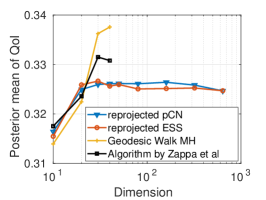
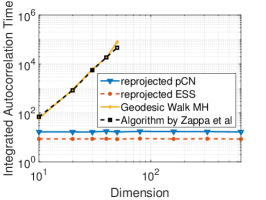
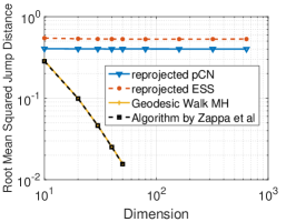
Figure 4.4: Estimated posterior mean (left), integrated autocorrelation time (middle) for $f$ as in (4.7) and root mean squared jump distance (right) for Algorithms 4, 5, 6 and 7 as applied to the Bayesian level set inverse problem.

4.2 Bayesian density estimation

We now consider a second application of Bayesian inference on high-dimensional spheres. We follow the approach of Holbrook et al. (2020) to nonparametric Bayesian density estimation: Given data $y_{1},\ldots,y_{n}\in D$, for $D$ a bounded smooth domain in $\mathbb{R}^{k}$, we infer the Lebesgue probability density function $p$ of the data, where $p$ belongs to

$$\mathrm{P}\coloneqq\left\{p\colon D\to[0,\infty)\,\middle|\,\int_{D}p(y)\,\mathrm{d}y=1\right\}.$$

The set $\mathrm{P}$ is the unit simplex in the Banach space $L^{1}(D)$. Instead of inferring $p$ directly, we instead infer the square root $g=\sqrt{p}$ of $p$, where $g$ belongs to

$$\mathrm{Q}\coloneqq\left\{g\colon D\to\mathbb{R}\,\middle|\,\int_{D}g^{2}(y)\,\mathrm{d}y=1\right\}.$$

The set $\mathrm{Q}$ coincides with the unit sphere of the function space $L^{2}(D)$.

Data.

We use the British coal mine disaster data set that was studied in Holbrook et al. (2020). This data set consists of the dates of $191$ disasters recorded between March 1851 and March 1962 which can be found in Hand et al. (1994, Data set 204). We aim to estimate the underlying probability density between the years 1850 and 1965. However, for computations and simplicity, we scale the data to lie within $D=[0,1]$ by a suitable affine transformation. Thus, we would like to infer a square root density $g\in\mathbb{S}=\mathrm{Q}$, where $\mathbb{S}$ denotes the unit sphere of $L^{2}([0,1])$.

Prior and posterior.

For numerical discretisation and constructing a prior model for $g$, we expand $g$ with respect to a suitable orthonormal system $\{\phi_{i}\mid i\in\mathbb{N}\}$ in $L^{2}(D)$, $D=[0,1]$. Here, we choose the same system as in (Holbrook et al., 2020) which is based on a mean-zero Gaussian process model for $g$ with a Whittle–Matérn covariance (cf. (4.6)):

$$g=g(\bar{X})=\sum_{i=1}^{\infty}\bar{X}_{i}\,\phi_{i},\qquad\phi_{1}\equiv 1,\;\;\phi_{i}(y)=\sqrt{2}\cos(\pi\,(i-1)\,y),\;i>1,$$ (4.9)

where $\bar{X}=(\bar{X}_{i})_{i\in\mathbb{N}}$ are suitable random coefficients almost surely belonging to the unit sphere in $\ell^{2}$, such that the resulting $g=g(\bar{X})$ belongs to the unit sphere in $L^{2}([0,1])$. Here, we assume as prior for $\bar{X}$ that $\bar{X}\sim\mathrm{ACG}(\Lambda)$ where $\Lambda=\mathrm{diag}(\lambda_{i}\colon i\in\mathbb{N})$ with $\lambda_{i}=\sigma^{2}(\kappa+\pi^{2}(i-1)^{2})^{-r}$, $i\geqslant 1$. We choose $\sigma=0.5$, $\kappa=0.1$ and $r=1$ for our experiments. We chose these parameter values because of their similarity to the values used by Holbrook et al. (2020). The resulting prior for $g$ is then $\mathrm{ACG}(C)$ where $C\colon L^{2}(D)\to L^{2}(D)$ denotes the covariance operator $Cv(y)=\int_{D}c(y,y^{\prime})v(y^{\prime})\,\mathrm{d}y^{\prime}$ using the corresponding covariance function

$$c(y,y^{\prime})=\sum_{i=0}^{\infty}\lambda_{i}\,\phi_{i}(y)\,\phi_{i}(y^{\prime}).$$

Given $g\in\mathrm{Q}$, the likelihood $L(y;g)$ for observing the data $y=(y_{1},\ldots,y_{n})\in D^{n}$ is

$$L(y;g)=\prod_{i=1}^{n}g^{2}(y_{i})=\exp\left(\sum_{j=1}^{n}\log(g^{2}(y_{j}))\right)=\exp\left(2\sum_{j=1}^{n}\log(|g(y_{j})|)\right).$$

Thus, using the series representation in (4.9), we obtain as likelihood for $y$ given coefficients $\bar{x}$ in the unit sphere of $\ell^{2}$,

$$L(y;\bar{x})=\exp\left(-\bar{\Phi}(\bar{x})\right),\qquad\bar{\Phi}(\bar{x})\coloneqq-2\sum_{j=1}^{n}\log\left(\left|\sum_{i=0}^{\infty}\bar{x}_{i}\,\phi_{i}(y_{j})\right|\right).$$

Note that $\bar{\Phi}\colon\ell^{2}\to\mathbb{R}$ is bounded. Given the data $y$, the resulting posterior for the coefficients $\bar{X}$ follows the form (3.2) with $\mu_{0}=\mathrm{ACG}(\Lambda)$, and the assumptions of Theorem 3.7 are satisfied.

A quantity of interest for this problem is the posterior expectation for the probability mass of $p$ between $0.435$ and $0.574$. This quantity of interest is the probability of a coal mine disaster between the years 1900 and 1916. It can be written as

$$f(\bar{x}) \coloneqq\int_{0.435}^{0.574}g^{2}(y,\bar{x})\,\mathrm{d}y=\left(\sum_{i,k=1}^{\infty}w_{i,k}\bar{x}_{i}\,\bar{x}_{k}\right)^{2}$$ (4.10)

where $w_{i,k}\coloneqq\int_{0.435}^{0.574}\phi_{i}(y)\,\phi_{k}(y)\,\mathrm{d}y$, i.e., $f$ is a quadratic function of $\bar{x}$.

MCMC simulations.

We truncated the expansion in (4.9) after $d$ terms for $d=10$, $20$, $30$, $40$, $50$, $100$, $200$, $400$, and $800$ and sampled approximately from the resulting truncated posterior $\mu^{(d)}$ on $\mathbb{S}^{d-1}$ for the coefficients $\bar{x}^{(d)}=(\bar{x}_{1},\ldots,\bar{x}_{d})$ using the prior $\mu^{(d)}_{0}=\mathrm{ACG}(\Lambda_{d})$ with $\Lambda_{d}\coloneqq\mathrm{diag}(\lambda_{1},\ldots,\lambda_{d})$. To this end, we applied the four MCMC algorithms described in Section 3, and used them to compute the expectation of the quantity $f$ in (4.10) with respect to the truncated posterior $\mu^{(d)}$. After a burn-in period of $10^{5}$ iterations, we ran the algorithms for $10^{6}$ iterations and compared their efficiency. We quantified their efficiency in terms of the estimated integrated autocorrelation time for $f$ and the root mean squared jump distance. We display the results in Figure 4.5. As in Figure 4.4, the results exhibit dimension-independent efficiency of the two reprojected MCMC methods, whereas the geodesic random walk-MH algorithm and the MH algorithm of Zappa et al. (2018) show a clear and drastic deterioration of efficiency as $d$ increases.

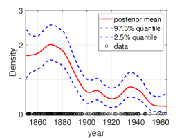
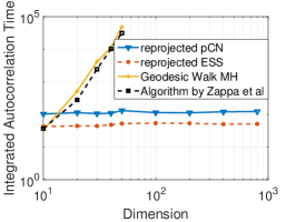
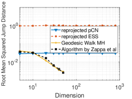
Figure 4.5: Estimated posterior mean and pointwise posterior quantiles for the density $p$ based on truncation of (4.9) to the first $d=30$ summands (left), estimated integrated autocorrelation time for quantity of interest $f$ as in (4.10) (middle), and root mean squared jump distance (right) for Algorithms 4, 5, 6 and 7 as applied to the Bayesian density estimation problem.

5 Closing remarks

In this paper, we proposed efficient MCMC algorithms for sampling target measures on high-dimensional spheres that are absolutely continuous with respect to an ACG prior. Our algorithms exploit the structure of the ACG prior by lifting the sampling problem on the sphere to a sampling problem in the ambient Hilbert space. This allows us to apply existing MCMC algorithms on linear spaces — such as the pCN-MH algorithm — for which there are theoretical results concerning dimension-independent efficiency.

Using the technique of push-forward Markov kernels, we then obtained transition kernels on the sphere that inherit many properties of the transition kernels in the ambient Hilbert space, e.g. reversibility with respect to the desired target measure. Under fairly mild conditions, we showed the uniform ergodicity of Markov chains generated by our algorithms, and provided theoretical arguments for the dimension independence of their spectral gaps.

Using binary classification and Bayesian density estimation as test problems, we compared the performance of our methods to that of MH algorithms based on the geodesic random walk proposal of Mangoubi and Smith (2018) and the approach of Zappa et al. (2018). Our results illustrated the robustness of our algorithms as the dimension of the state space increased. In comparison, the statistical efficiency of the two other existing algorithms decreased as the dimension of the state space increased.

Based on our work, several interesting questions for future research remain. A theoretical analysis of the dimension independence of the (reprojected) ESS transition kernel remains an open issue. Here Markov chain comparison techniques — as have been developed by, for example, Peskun (1973), Andrieu and Vihola (2016), and Rudolf and Sprungk (2018) — may be useful for establishing the inheritance of a spectral gap from the pCN-MH transition kernel to the ESS transition kernel. Additionally, it seems promising to modify our algorithms so that they can be applied to sample from target measures with respect to other common priors such as Bingham distributions, by using the acceptance-rejection approach of Kent et al. (2018), for example.

Appendix A Gaussian measures and angular central Gaussian measures

A.1 Gaussian measures on Hilbert spaces

We first briefly recall some basic notions related to measures, especially Gaussian measures, on Hilbert spaces. A standard reference in this area is the book of Bogachev [1998].

In the following, we consider a separable Hilbert space $\mathbb{H}$ with norm $\|\hbox to5.71527pt{\hss$\cdot$\hss}\|$ and inner product $\langle\hbox to5.71527pt{\hss$\cdot$\hss},\hbox to5.71527pt{\hss$\cdot$\hss}\rangle$. Suppose $\mu\in\mathcal{P}(\mathbb{H})$ with finite second moment $\int_{\mathbb{H}}\|x\|^{2}\,\mu(\mathrm{d}x)$ is given. Then the mean element $a\in\mathbb{H}$ and covariance operator $C\colon\mathbb{H}\to\mathbb{H}$ of $\mu$ are determined by

$$0 =\int_{\mathbb{X}}\langle v,x-a\rangle\,\mu(\mathrm{d}x) v\in\mathbb{H}$$ for all , (A.1)

$$\langle Cu,v\rangle =\int_{\mathbb{X}}\langle u,x-a\rangle\langle v,x-a\rangle\,\mu(\mathrm{d}x) u,v\in\mathbb{H}$$ for all . (A.2)

When $a=0$, the measure $\mu$ is said to be centred.

In this paper, we focus on Gaussian measures $\mu=\mathrm{N}(a,C)$ on $\mathbb{H}$. Such measures are equivalently determined by the property that every one-dimensional linear image is Gaussian on $\mathbb{R}$, i.e. identifying $\ell\in\mathbb{H}$ with the continuous linear functional $\mathbb{H}\to\mathbb{R}$, $x\mapsto\langle\ell,x\rangle$,

$$\mu=\mathrm{N}(a,C)\in\mathcal{P}(\mathbb{H})\iff\forall\ell\in\mathbb{H},\;\ell_{\sharp}\mu=\mathrm{N}(\langle\ell,a\rangle,\langle C\ell,\ell\rangle)\in\mathcal{P}(\mathbb{R});$$

or by the form of the characteristic function, i.e.

$$\mu=\mathrm{N}(a,C)\in\mathcal{P}(\mathbb{H})\iff\forall v\in\mathbb{H},\;\int_{\mathbb{X}}\exp(i\langle v,x\rangle)\,\mu(\mathrm{d}x)=\exp\bigl{(}i\langle v,a\rangle-\tfrac{1}{2}\langle Cv,v\rangle\bigr{)}.$$

The covariance operator $C$ of a probability measure on $\mathbb{H}$ is always self-adjoint and positive semi-definite, and so its eigenvalues are all real and non-negative. Furthermore, the assumption of finite second moment implies that these eigenvalues are summable, i.e. $C$ is a trace-class operator.

Given any self-adjoint and positive-definite operator $C\colon\mathbb{H}\to\mathbb{H}$, we define for $x,y\in\operatorname{ran}(C^{1/2})$ the weighted inner product and norm

$$\langle x,y\rangle_{C} \coloneqq\langle C^{-1/2}x,C^{-1/2}y\rangle,$$ (A.3)

$$\|x\|_{C} \coloneqq\sqrt{\langle x,x\rangle_{C}},$$ (A.4)

If $C$ is the covariance operator of a Gaussian measure $\mu=\mathrm{N}(a,C)$, then $\operatorname{ran}(C^{1/2})$ is the Cameron–Martin space of $\mu$, and (A.3) and (A.4) are often called the precision inner product and norm respectively.

The topological support of $\mathrm{N}(0,C)$ — i.e. the smallest closed set of full measure — is the closure in $\mathbb{H}$ of $\operatorname{ran}(C)$ [Bogachev, 1998, Theorem 3.6.1]. A sufficient condition for the density of $\operatorname{ran}(C)$ in $\mathbb{H}$ is the strict positivity of $C$, i.e. that it has no null eigenvalue. The containments $\operatorname{ran}(C)\subseteq\operatorname{ran}(C^{1/2})\subseteq\mathbb{H}$ always hold, and are strict when the Cameron–Martin space $\operatorname{ran}(C^{1/2})$ has infinite dimension.

A.2 Angular central Gaussian measures on spheres in Hilbert spaces

We denote the unit sphere in a separable Hilbert space $\mathbb{H}$ by

$$\mathbb{S}\coloneqq\{x\in\mathbb{H}\mid\|x\|=1\}.$$

If $\mathbb{H}=\mathbb{R}^{d}$, then we emphasise the dimension and denote the unit sphere by $\mathbb{S}^{d-1}$. The sphere $\mathbb{S}$ is equipped with the following metric $d_{\mathbb{S}}\colon\mathbb{S}\times\mathbb{S}\to[0,\pi]$:

$$d_{\mathbb{S}}(\bar{x},\bar{y})\coloneqq\arccos\left(\langle\bar{x},\bar{y}\rangle\right)=2\arcsin\left(\frac{1}{2}\|\bar{x}-\bar{y}\|\right)\qquad\bar{x},\bar{y}\in\mathbb{S},$$ (A.5)

where the second identity follows from elementary trigonometry. The definition of $d_{\mathbb{S}}$ by the arcsine function also extends to the unit sphere $\mathbb{S}$ in general Banach spaces. Moreover, it yields the Lipschitz equivalence — and hence the topological equivalence — of $d_{\mathbb{S}}$ and the metric on $\mathbb{S}$ induced by the norm $\|\hbox to5.71527pt{\hss$\cdot$\hss}\|$ of the ambient space $\mathbb{H}$:

$$\|\bar{x}-\bar{y}\|\leqslant d_{\mathbb{S}}(\bar{x},\bar{y})\leqslant\frac{\pi}{2}\|\bar{x}-\bar{y}\|\qquad\forall\bar{x},\bar{y}\in\mathbb{S},$$ (A.6)

since $g(r)=2\arcsin\left(\frac{1}{2}r\right)/r$ varies between $1$ and $\pi/2$ for $r\in[0,2]$. Thus, the metric $d_{\mathbb{S}}$ is topologically equivalent to the norm of the ambient space on $\mathbb{S}$. We record this result in Lemma A.1 below. According to Kechris [1995, Proposition 3.3(ii)], a closed subset of a Polish space is always itself Polish in the relative (subspace) topology. Thus, $(\mathbb{S},d_{\mathbb{S}})$ is a Polish space and $\mathcal{B}(\mathbb{S})=\{B\cap\mathbb{S}\mid B\in\mathcal{B}(\mathbb{H})\}$.

Lemma A.1.

The topology on $\mathbb{S}$ generated by $d_{\mathbb{S}}$ coincides with the relative topology on $\mathbb{S}$ generated by the norm $\|\hbox to5.71527pt{\hss$\cdot$\hss}\|$ of $\mathbb{H}$.

Proof. This is a consequence of the Lipschitz equivalence of the metrics (A.6). $\blacksquare$

Fix an arbitrary $\bar{z}\in\mathbb{S}$. Recall the radial projection to the sphere defined in (3.1),

$$\Pi^{\mathbb{S}}\colon\mathbb{H}\to\mathbb{S},\quad\Pi^{\mathbb{S}}(x)\coloneqq\begin{cases}\frac{x}{\|x\|},&\text{if $x\neq 0$,}\\ \bar{z},&\text{if $x=0$.}\end{cases}$$

The choice of $\bar{z}$ is not important in what follows, but we fix $\bar{z}$ in order to ensure that $\Pi^{\mathbb{S}}$ is a measurable mapping from $\mathbb{H}$ into $\mathbb{S}$.

Recall that the ACG measure on $\mathbb{S}$ associated to a centred Gaussian measure $\mathrm{N}(0,C)$ on $\mathbb{H}$ is given by

$$\mu\coloneqq\Pi^{\mathbb{S}}_{\sharp}\mathrm{N}(0,C)$$

and denoted by $\mu=\mathrm{ACG}(C)$. In other words, under $\mathrm{ACG}(C)$, each $E\in\mathcal{B}(\mathbb{S})$ is assigned the Gaussian $\mathrm{N}(0,C)$-measure of the cone $\{\alpha u\in\mathbb{X}\mid\alpha>0,u\in E\}$. Note that $\mathrm{ACG}(C)=\mathrm{ACG}(\lambda C)$ for $\lambda\neq 0$ and so it can sometimes be useful to fix a normalisation for $C$, e.g. by taking its leading eigenvalue to be unity.

Corollary A.2.

Let $C_{E}\coloneqq\{\alpha e\mid\alpha>0,e\in E\}\subseteq\mathbb{H}$ denote the cone spanned by a subset $E\subseteq\mathbb{S}$. The set $E$ is open in $(\mathbb{S},d_{\mathbb{S}})$ if and only if $C_{E}$ is open in $(\mathbb{H},\|\hbox to5.71527pt{\hss$\cdot$\hss}\|)$.

Proof. Suppose that $C_{E}$ is open in $\mathbb{H}$. Then $E=C_{E}\cap\mathbb{S}$ is, by Lemma A.1, open in $(\mathbb{S},d_{\mathbb{S}})$.

Let $\Pi^{\mathbb{S}}|_{\mathbb{H}\setminus\{0\}}$ be the restriction of the radial projection $\Pi^{\mathbb{S}}$ defined in (3.1) to $\mathbb{H}\setminus\{0\}$. For $E$ in $(\mathbb{S},d_{\mathbb{S}})$, $(\Pi^{\mathbb{S}}|_{\mathbb{H}\setminus\{0\}})^{-1}(E)=C_{E}$. Equip $\mathbb{H}\setminus\{0\}$ with the subspace topology. Then $\Pi^{\mathbb{S}}|_{\mathbb{H}\setminus\{0\}}$ is continuous, and if $E$ is open, then $C_{E}$ is open in $(\mathbb{H}\setminus\{0\},\|\hbox to5.71527pt{\hss$\cdot$\hss}\|)$, and hence in $(\mathbb{H},\|\hbox to5.71527pt{\hss$\cdot$\hss}\|)$. $\blacksquare$ Whenever $\mathrm{N}(0,C)$ has support equal to $\mathbb{H}$, Corollary A.2 immediately implies that the induced $\mathrm{ACG}(C)$ measure has support equal to $\mathbb{S}$; thus, in view of Section A.1, $\mathrm{ACG}(C)$ is a strictly positive measure on $\mathbb{S}$ whenever $C$ is positive definite.

In the case where $\mathbb{H}=\mathbb{R}^{d}$ with the usual Euclidean norm and $C\in\mathbb{R}^{d\times d}$ is symmetric and positive definite, one can show that the density $\rho\colon\mathbb{S}^{d-1}\to[0,\infty)$ of $\mu=\mathrm{ACG}(C)$ with respect to the $(d-1)$-dimensional Hausdorff measure on the sphere is

$$\rho(\bar{x}) =\int_{0}^{\infty}\frac{\exp(-\tfrac{1}{2}(r\bar{x})\cdot C^{-1}(r\bar{x}))}{\sqrt{\det(2\pi C)}}r^{d-1}\,\mathrm{d}r$$

$$=\frac{\Gamma(d/2)}{2(\tfrac{1}{2}\|\bar{x}\|_{C}^{2})^{d/2}\sqrt{\det(2\pi C)}}$$

$$=\frac{\Gamma(d/2)}{2\pi^{d/2}\sqrt{\det C}}\|\bar{x}\|_{C}^{-d}.$$

In the second equation, we used the fact that, for $a>0$ and $n\in\mathbb{N}$, $\int_{0}^{\infty}a^{-r^{2}}r^{n-1}\,\mathrm{d}r=\frac{\Gamma(n/2)}{2(\log a)^{n/2}}$ [e.g. Tyler, 1987, Equation (1)].

Remark A.3.

The above definitions and properties can be readily adapted to the image of a centred Gaussian measure on a projective space, i.e. the quotient of $\mathbb{H}$ by the equivalence relation $u\sim v\iff u=\lambda v$ for some $\lambda\neq 0$, i.e. $\mathbb{S}$ with antipodal points identified. Note that, while $\mathrm{ACG}(C)$ on $\mathbb{S}$ is always a multimodal distribution with at least two modes, its image on the projective space can be unimodal, which may be desirable in applications.

Appendix B Markov chain Monte Carlo

Markov chain methods provide a standard tool for approximate sampling of complicated distributions, such as posterior distributions appearing in the Bayesian analysis of data. We recall here notions related to MCMC on a general state space $\mathbb{X}$ equipped with a target probability measure $\mu\in\mathcal{P}(\mathbb{X})$, the Metropolis–Hastings and slice sampling paradigms, and make some particular points about MCMC on infinite-dimensional Hilbert spaces.

B.1 General notions

By a Markov kernel on a topological space $\mathbb{X}$ we mean a function $K\colon\mathbb{X}\times\mathcal{B}(\mathbb{X})\to[0,1]$ such that $K(x,\hbox to5.71527pt{\hss$\cdot$\hss})\in\mathcal{P}(\mathbb{X})$ for each $x\in\mathbb{X}$, and $K(\hbox to5.71527pt{\hss$\cdot$\hss},A)$ is a measurable function for each $A\in\mathcal{B}(X)$. A sequence of random variables $(X_{n})_{n\in\mathbb{N}}$, mapping from $(\Omega,\mathcal{A},\mathbb{P})$ to $\mathbb{X}$, is a (time-homogeneous) Markov chain with transition kernel $K$ on $\mathbb{X}$ if

$$\mathbb{P}(X_{n+1}\in A\mid X_{1},\dots,X_{n})=\mathbb{P}(X_{n+1}\in A\mid X_{n})=K(X_{n},A),\quad n\in\mathbb{N},\,A\in\mathcal{B}(\mathbb{X}),$$

where $K$ is a Markov kernel. We abuse notation and also use $K$ to denote the transition operator induced by the kernel $K$; the transition operator acts on functions $f\colon\mathbb{X}\to\mathbb{R}$ via

$$(Kf)(x)\coloneqq\int_{\mathbb{X}}f(y)\,K(x,\mathrm{d}y)=\mathbb{E}\left[f(X_{n+1})\mid X_{n}=x\right]\quad\text{for $x\in\mathbb{X}$.}$$ (B.1)

The idea of MCMC is to construct a Markov chain $(X_{n})_{n\in\mathbb{N}}$ with transition kernel $K$ such that the distribution of $X_{n}$ converges to $\mu$ as $n\to\infty$. Ideally, this convergence will be “fast” and the correlation between successive random variables $X_{n}$ and $X_{n+1}$ will also be weak.

A necessary condition for a transition kernel $K$ to have $\mu$ as a limiting distribution is that $\mu$ is an invariant distribution of $K$, i.e.

$$\mu(A)=\mu K(A)\coloneqq\int_{\mathbb{X}}K(x,A)\,\mu(\mathrm{d}x),\quad\text{for all $A\in\mathcal{B}(\mathbb{X})$.}$$ (B.2)

Reversibility (or detailed balance) of a transition kernel $K$ on $\mathbb{X}$ with respect to $\mu$ refers to the property that

$$K(x,\mathrm{d}y)\mu(\mathrm{d}x)=K(y,\mathrm{d}x)\mu(\mathrm{d}y),$$ (B.3)

i.e. that the measure $K(x,\mathrm{d}y)\mu(\mathrm{d}x)$ on $\mathbb{X}\times\mathbb{X}$ is symmetric. If (B.3) holds we say that $K$ is $\mu$-reversible. Reversibility of a transition kernel $K$ with respect to $\mu$ implies that $K$ has $\mu$ as an invariant distribution, although the converse is generally false.

If $\mu$ is an invariant distribution of $K$, and if some non-restrictive regularity conditions such as $\varphi$-irreducibility and Harris recurrence hold, then a strong law of large numbers holds, i.e.

$$\lim_{n\to\infty}\frac{1}{N}\sum_{n=1}^{N}f(X_{n})=\int_{\mathbb{X}}f(x)\,\mu(\mathrm{d}x)\quad\mathbb{P}\text{-a.s.},$$

for any $\mu$-integrable $f\colon\mathbb{X}\to\mathbb{R}$ [Meyn and Tweedie, 2009, Asmussen and Glynn, 2011]. This shows that the “MCMC-time average” $\frac{1}{N}\sum_{n=1}^{N}f(X_{n})$ can be used to approximate the mean of $f$ with respect to the distribution of interest $\mu$. For more quantitative statements the spectral gap of a Markov chain (or its transition kernel) is a crucial quantity. For a transition kernel $K$ that is reversible with respect to $\mu$ (inducing the transition operator $K$ via (B.1)) we define

$$\operatorname{gap}_{\mu}(K)\coloneqq 1-\|K\|_{L^{2}_{0,\mu}\to L^{2}_{0,\mu}},$$ (B.4)

where we recall that $L^{2}_{0,\mu}\coloneqq\{f\in L^{2}(\mu)\mid\int f(u)\,\mu(\mathrm{d}u)=0\}$ and where $\|K\|_{L^{2}_{0,\mu}\to L^{2}_{0,\mu}}$ denotes the norm of the operator $K$, which we view as an element of the space of bounded linear operators from $L^{2}_{0,\mu}$ to itself. An $L^{2}_{\mu}$-spectral gap, that is, $\operatorname{gap}_{\mu}(K)>0$, leads to desirable properties of a Markov chain $(X_{n})_{n\in\mathbb{N}}$ with transition kernel $K$. For instance, it implies a central limit theorem, see e.g. [Douc et al., 2018, Section 22.5] and the relevant references therein. In particular, an explicit lower bound on $\operatorname{gap}_{\mu}(K)$ leads to an estimate of the total variation distance and a mean squared error bound of the time average $\frac{1}{N}\sum_{n=1}^{N}f(X_{n})$. More precisely, it is well known, e.g. by virtue of [Novak and Rudolf, 2014, Lemma 2 and Lemma 3], that

$$\|\xi K^{n}-\mu\|_{\mathrm{TV}}\leqslant(1-\operatorname{gap}_{\mu}(K))^{n}\left\|\frac{\mathrm{d}\xi}{\mathrm{d}\mu}-1\right\|_{L^{2}_{\mu}},$$ (B.5)

where $\|\xi K^{n}-\mu\|_{\mathrm{TV}}\coloneqq\sup_{A\in\mathcal{B}(\mathbb{X})}|\xi K^{n}(A)-\mu(A)|$ denotes the total variation distance between $\xi K^{n}=\mathbb{P}_{X_{n+1}}$ and $\mu$, $\xi\coloneqq\mathbb{P}_{X_{1}}$, and $\|f\|_{L^{p}_{\mu}}^{p}\coloneqq\int_{\mathbb{X}}|f|^{p}\,\mathrm{d}\mu$ for $f\colon\mathbb{X}\to\mathbb{R}$. Furthermore, Rudolf [2012] shows that, for every $p>2$, there exists an explicit constant $c_{p}$ such that, for $f\in L^{p}(\mu)$ with $\|f\|^{p}_{L^{p}_{\mu}}\leqslant 1$,

$$\mathbb{E}\left[\left|\frac{1}{N}\sum_{n=1}^{N}f(X_{n})-\int_{\mathbb{X}}f{\mathrm{d}}\mu\right|^{2}\right]\leqslant\frac{2}{N\cdot\operatorname{gap}_{\mu}(K)}+\frac{c_{p}\left\|\frac{\mathrm{d}\xi}{\mathrm{d}\mu}-1\right\|_{\infty}}{N^{2}\cdot\operatorname{gap}_{\mu}(K)^{2}}.$$

There are also other non-asymptotic bounds that consider different convergence assumptions on the Markov chain and the underlying error criterion. For details we refer to [Łatuszyński and Niemiro, 2011, Łatuszyński et al., 2013, Rudolf and Schweizer, 2015, Paulin, 2015, Fan et al., 2021] and the references therein.

In the following we briefly discuss two popular methods for the construction of a transition kernel $K$ that is reversible with respect to $\mu$.

B.2 Metropolis–Hastings (MH) algorithms

Probably the most popular method for constructing a transition kernel that is reversible with respect to $\mu$ is given by the MH algorithm. Given a Markov kernel $Q$ on $\mathbb{X}$ which serves as a proposal mechanism, i.e. a ‘proposal kernel’, and given a function $\alpha\colon\mathbb{X}\times\mathbb{X}\to[0,1]$ which provides acceptance probabilities and depends on $\mu$ and $Q$, a transition from a state $x$ to a state $y$ in the MH algorithm proceeds as follows.

Transition Mechanism B.1 (Metropolis–Hastings).

Let $Q$ be a proposal kernel and $\alpha\colon\mathbb{X}\times\mathbb{X}\to[0,1]$ be an acceptance probability function. Given the current state $x\in\mathbb{X}$, one obtains the next state $y\in\mathbb{X}$ as follows:

1. Draw $X^{\prime}\sim Q(x,\hbox to5.71527pt{\hss$\cdot$\hss})$ and $U\sim\mathrm{U}[(0,1)]$ independently and denote the realisations by $x^{\prime}$ and $u$ respectively;

2. If $u<\alpha(x,x^{\prime})$, return $y\coloneqq x^{\prime}$, otherwise return $y\coloneqq x$.

The algorithm above can be rewritten as a transition kernel:

$$K(x,\mathrm{d}y)=\alpha(x,y)Q(x,\mathrm{d}y)+r(x)\delta_{x}(\mathrm{d}y),\qquad r(x)\coloneqq 1-\int_{\mathbb{X}}\alpha(x,y)\,Q(x,\mathrm{d}y),$$ (B.6)

where $\delta_{x}$ denotes the Dirac measure on $\mathbb{X}$ at $x\in\mathbb{X}$ and the function $r$ is called the ‘rejection probability’. It remains to specify $\alpha$. Let $\sigma^{+},\sigma^{-}\in\mathcal{P}(\mathbb{X}\times\mathbb{X})$ with

$$\sigma^{+}(\mathrm{d}x,\mathrm{d}x^{\prime}) \coloneqq Q(x,\mathrm{d}x^{\prime})\mu(\mathrm{d}x),$$ (B.7)

$$\sigma^{-}(\mathrm{d}x,\mathrm{d}x^{\prime}) \coloneqq\sigma^{+}(\mathrm{d}x^{\prime},\mathrm{d}x)=Q(x^{\prime},\mathrm{d}x)\mu(\mathrm{d}x^{\prime}),$$

and set

$$\alpha(x,x^{\prime}) \coloneqq\min\left\{1,\frac{\mathrm{d}\sigma^{-}}{\mathrm{d}\sigma^{+}}(x,x^{\prime})\right\}.$$

Then the transition kernel $K$ defined in (B.6) is reversible with respect to $\mu$ [Tierney, 1998]. Of course, the Radon–Nikodym derivative $\frac{\mathrm{d}\sigma^{-}}{\mathrm{d}\sigma^{+}}(x,x^{\prime})$ does not necessarily exist. In the finite-dimensional Euclidean setting where $\mathbb{X}=\mathbb{R}^{d}$, the derivative $\frac{\mathrm{d}\sigma^{-}}{\mathrm{d}\sigma^{+}}$ is often just the ratio of Lebesgue densities. However, in infinite-dimensional spaces the absolute continuity $\sigma^{-}\ll\sigma^{+}$ requires the choice of a suitable proposal kernel $Q$.

B.3 Slice sampling

Suppose that a $\sigma$-finite reference measure $\mu_{0}$ on $\mathbb{X}$ is given that satisfies $\mu\ll\mu_{0}$. Additionally, we assume that the probability density function $\frac{\mathrm{d}\mu}{\mathrm{d}\mu_{0}}$ satisfies

$$\frac{\mathrm{d}\mu}{\mathrm{d}\mu_{0}}(x)\propto\exp(-\Phi(x)),\quad\mu_{0}\text{-a.e.\ }x\in\mathbb{X},$$

for a measurable function $\Phi\colon\mathbb{X}\to\mathbb{R}$ such that $\exp(-\Phi)$ is integrable with respect to $\mu_{0}$. For some $s>0$, define

$$\mathbb{X}_{s}\coloneqq\{x\in\mathbb{X}\mid\exp(-\Phi(x))\geqslant s\},$$ (B.8)

to be the super-level set of $\exp(-\Phi)$ to level $s$. Let $\|\exp(-\Phi)\|_{\infty}\coloneqq\mathop{\mu_{0}\text{-ess\,}\sup}\limits_{x\in\mathbb{X}}|\exp(-\Phi(x))|$ and note that $\mu_{0}(\mathbb{X}_{s})\in(0,\infty)$ for $s\in(0,\|\exp(-\Phi)\|_{\infty})$. Here,

$$\mathop{\mu_{0}\textup{-ess\,sup}}\limits_{x\in\mathbb{X}}f(x)$$

denotes the essential supremum with respect to $\mu_{0}$ of $f\colon\mathbb{X}\to\mathbb{R}$. Define the probability measure $\mu_{0,s}\in\mathcal{P}(\mathbb{X})$ by

$$\mu_{0,s}(A)\coloneqq\frac{\mu_{0}(A\cap\mathbb{X}_{s})}{\mu_{0}(\mathbb{X}_{s})},\quad A\in\mathcal{B}(\mathbb{X}),$$

that is, $\mu_{0,s}$ is the normalised restriction of $\mu_{0}$ to $\mathbb{X}_{s}$. In the idealised slice sampling algorithm, a transition from a state $x$ to a state $y$ proceeds as follows.

Transition Mechanism B.2 (Idealised slice sampling).

Given the current state $x\in\mathbb{X}$ one obtains the next state $y\in\mathbb{X}$ as follows:

1. Draw $S\sim\mathrm{U}[(0,\exp(-\Phi(x)))]$ and let $s$ be the realisation.

2. Draw $Y\sim\mu_{0,s}$ and let the state $y$ be the realisation of $Y$.

The corresponding transition kernel takes the form

$$K(x,\mathrm{d}y)=\frac{1}{\exp(-\Phi(x))}\int_{0}^{\exp(-\Phi(x))}\mu_{0,s}(\mathrm{d}y)\,\mathrm{d}s,$$

and it can be readily shown that $K$ is reversible with respect to $\mu$.

Remark B.3.

In the case that $\mathbb{X}=\mathbb{R}^{d}$ and $\mu_{0}$ is the Lebesgue measure, $\mu_{0,s}$ coincides with the uniform distribution on $\mathbb{X}_{s}$. In that setting the corresponding method is known as simple (uniform) slice sampling and recent results [Natarovskii et al., 2021b, Theorem 3.10] concerning the spectral gap indicate under which conditions robust convergence behaviour with respect to the dimension is present.

However, the main issue with the idealised slice sampling algorithm is that the second step in Transition Mechanism B.2 may be difficult to implement, because the implicit assumption of being able to draw samples from $\mu_{0,s}$ for an arbitrary level $s$ may be very restrictive. Whenever one is not able to sample from a distribution exactly, one can try to use a suitable Markov chain step. Namely, one substitutes the second step of Transition Mechanism B.2 by performing a transition, depending on $x$ and $t$, which (at least) has stationary distribution $\mu_{0,s}$. Such approaches are known as hybrid slice sampling strategies; see e.g. [Łatuszyński and Rudolf, 2014] for some theory and comparison results. There are several different methods in the literature that are feasible in finite-dimensional settings, and can — from an algorithmic perspective — be lifted to infinite-dimensional scenarios; see e.g. [Neal, 2003, Murray et al., 2010, Li and Walker, 2023].

Appendix C Two random walk-like MCMC algorithms on $\mathbb{S}^{d-1}$

We describe now two MH algorithms from the literature. These algorithms use random walk-like proposals that are defined on general, finite-dimensional manifolds $\mathbb{M}$. We shall compare the algorithms described in Section 3.2 with these algorithms on a numerical example in Section 4. In the following paragraphs we first describe the corresponding MH algorithm for a general manifold $\mathbb{M}$ and then provide the particular algorithm for the case of sampling on a sphere $\mathbb{M}=\mathbb{S}^{d-1}$. Throughout, we assume that $\mathbb{M}$ admits a Hausdorff measure $\mathcal{H}_{\mathbb{M}}$ and that the target probability measure $\mu$ on $\mathbb{M}$ is given by an unnormalised density $\rho$ with respect to $\mathcal{H}_{\mathbb{M}}$, that is,

$$\frac{\mathrm{d}\mu}{\mathrm{d}\mathcal{H}_{\mathbb{M}}}(\bar{x})\propto\rho(\bar{x}),\qquad\bar{x}\in\mathbb{M}.$$ (C.1)

When $\mathbb{M}=\mathbb{S}^{d-1}$ and $\mu$ is a posterior measure with respect to an ACG prior $\mu_{0}=\mathrm{ACG}(C)$ as in (3.2),

$$\rho(\bar{x})=\frac{\exp(-\bar{\Phi}(\bar{x}))}{\|\bar{x}\|^{d}_{C}}.$$

Geodesic random walk-MH algorithm.

Assume that $\mathcal{H}_{\mathbb{M}}(\mathbb{M})<\infty$. Then the uniform measure $\mathrm{U}(\mathbb{M})$ on $\mathbb{M}$ is defined via $\mathrm{U}(\mathbb{M})(A)\coloneqq\mathcal{H}_{\mathbb{M}}(A)/\mathcal{H}_{\mathbb{M}}(\mathbb{M})$ for $A\in\mathcal{B}(\mathbb{M})$. The geodesic random walk as described in [Mangoubi and Smith, 2018] yields a Markov chain $(\bar{X}_{k})_{k\in\mathbb{N}}$ on $\mathbb{M}$ with $\mathrm{U}(\mathbb{M})$ as its limit distribution. For any $\bar{x}\in\mathbb{M}$, denote the tangent space at $\bar{x}$ by $\mathcal{T}_{\bar{x}}\mathbb{M}$, and for any vector $v\in\mathcal{T}_{\bar{x}}\mathbb{M}$, denote by $\gamma_{\bar{x},v}$ the unique geodesic $\gamma_{\bar{x},v}\colon[0,\infty)\to\mathbb{M}$ on $\mathbb{M}$ that satisfies $\gamma_{\bar{x},v}(0)=\bar{x}$ and $\gamma^{\prime}_{\bar{x},v}(0)=v$, where $\gamma^{\prime}$ denotes the first derivative.

Next, we present how a transition from a state $\bar{x}$ to a state $\bar{y}$ proceeds in the geodesic random walk algorithm.

Transition Mechanism C.1 (Geodesic random walk).

Given the current state $\bar{x}\in\mathbb{M}$ one obtains the next state $\bar{y}\in\mathbb{M}$ for fixed $t>0$ as follows:

1. Draw from the uniform distribution on the unit sphere in $\mathcal{T}_{\bar{x}}\mathbb{M}$ and call the result $v$;

2. Set $\bar{y}=\gamma_{\bar{x},v}(t)$.

Hence, in order to sample approximately from $\mu$ as in (C.1), we can employ the geodesic random walk kernel as a proposal kernel in an MH algorithm. The resulting acceptance probability $\alpha$ involves ratios of the unnormalised density $\rho$ in (C.1). Goyal and Shetty [2019, Theorem 27] argue that the corresponding geodesic random walk transition kernel is reversible with respect to $\mathrm{U}(\mathbb{M})$. Therefore, the resulting algorithm for realising the Metropolised geodesic random walk on $\mathbb{M}=\mathbb{S}^{d-1}$ is given as in Algorithm 6.

Remark C.2.

In order to sample from the uniform distribution on the unit sphere in $\mathcal{T}_{\bar{x}}\mathbb{M}$ we can use the tools outlined by Zappa et al. [2018] for the case of constrained $m$-dimensional manifolds embedded into $\mathbb{R}^{d}$, $d>m$, via

$$\mathbb{M}=\left\{x\in\mathbb{R}^{d}\,\middle|\,q_{i}(x)=0\quad\forall i=1,\ldots,L\right\},\qquad L\geqslant d-m,$$ (C.2)

where $q_{i}\colon\mathbb{R}\to\mathbb{R}$ are smooth functions. In particular, an orthonormal basis (ONB) of $\mathcal{T}_{\bar{x}}\mathbb{M}$ can be obtained by a QR decomposition of the Jacobian of $Q(x)\coloneqq(q_{1}(x),\ldots,q_{L}(x))$ evaluated at $x=\bar{x}$. Let us denote such a basis by $u_{1},\ldots,u_{m}\in\mathbb{R}^{d}$ and store the vectors in the columns of $U_{\bar{x}}=[u_{1}\mid\ldots\mid u_{m}]\in\mathbb{R}^{d\times m}$. Drawing a sample $w$ from $\mathrm{U}(\mathbb{S}^{m-1})$ and setting $v=U_{\bar{x}}w$ yields a sample according to the uniform distribution on the sphere in $\mathcal{T}_{\bar{x}}\mathbb{M}$. If $\mathbb{M}=\mathbb{S}^{d-1}$, then there is only one constraint function, i.e. $q_{1}(x)=\|x\|^{2}-1$. Hence, the tangent space $\mathcal{T}_{\bar{x}}\mathbb{M}$ coincides with the orthogonal complement $\bar{x}^{\perp}$ of $\operatorname*{span}\{\bar{x}\}$.

Algorithm 6 Geodesic random walk-MH on $\mathbb{S}^{d-1}$ [Mangoubi and Smith, 2018]

1:  Given: time $t\in(0,\frac{\pi}{2}]$ and initial state $\bar{x}_{0}\in\mathbb{S}^{d-1}$

2:  for $k\in\mathbb{N}_{0}$ do

3:     Compute ONB matrix $U_{{\bar{x}}_{k}}\in\mathbb{R}^{d\times(d-1)}$ of $\bar{x}_{k}^{\perp}$ according to Remark C.2

4:     Draw a sample $w_{k}$ from $\mathrm{U}(\mathbb{S}^{d-2})$ and set $v_{k}\coloneqq U_{{\bar{x}}_{k}}w_{k}$

5:     Set $\bar{y}_{k+1}\coloneqq\cos(t)\bar{x}_{k}+\sin(t)v_{k}$

6:     Compute $a\coloneqq\min\{1,\rho(\bar{y}_{k+1})/\rho(\bar{x}_{k})\}$

7:     Draw a sample $u$ from $\mathrm{U}([0,1])$

8:     if $u\leqslant a$ then

9:        Set $\bar{x}_{k+1}=\bar{y}_{k+1}$

10:     else

11:        Set $\bar{x}_{k+1}=\bar{x}_{k}$

12:     end if

13:  end for

Remark C.3 (Ergodicity).

In [Mangoubi and Smith, 2018, Theorem 7.1] it is shown that the geodesic random walk, i.e. the proposal kernel of Algorithm 6, possesses a mixing time with respect to a Wasserstein distance that depends only on the positive curvature of the manifold $\mathbb{M}$, given a suitably small integration time $t$. Thus, in case of the sphere $\mathbb{M}=\mathbb{S}^{d-1}$, the mixing time is independent of the dimension $d$ for any $t\in(0,\frac{\pi}{2}]$. However, this statement solely holds for the proposal chain. As we will see in Section 4, the MH algorithm based on the geodesic random walk proposal shows deteriorating efficiency as $d\to\infty$. Besides that, also the uniform ergodicity of Algorithm 6, or the geodesic random walk itself, is not obvious and left open for future research.

MH algorithm by Zappa et al. [2018].

The MH algorithm presented in [Zappa et al., 2018] shows some similarities with our method, in the sense that it first proposes a new state in the ambient Euclidean space which is then projected to the manifold $\mathbb{M}$. The manifold $\mathbb{M}$ is assumed to be of the form (C.2). Given a current state $\bar{x}\in\mathbb{M}$, we first draw a tangent vector $v\in\mathcal{T}_{\bar{x}}\mathbb{M}$, but this time with respect to an isotropic multivariate Gaussian measure $\mathrm{N}(0,s^{2}I_{d-m})$. Here, we can employ again the technique explained in Remark C.2, by using an ONB matrix $U_{\bar{x}}\in\mathbb{R}^{d\times(d-m)}$ of $\mathcal{T}_{\bar{x}}\mathbb{M}$, drawing $w$ from $\mathrm{N}(0,s^{2}I_{d-m})$, and defining the resulting sample $v=U_{\bar{x}}w$. We then consider $x\coloneqq\bar{x}+v\in\mathbb{R}^{d}$, and project $x$ to some $\bar{y}\in\mathbb{M}$ by

$$\bar{y}\coloneqq x+w\quad\text{ with suitable }\quad w\in\left(\mathcal{T}_{\bar{x}}\mathbb{M}\right)^{\perp}.$$

In general, computing $w$ and $\bar{y}$ requires solving a nonlinear system; see [Zappa et al., 2018, Equation (2.5)]. For $\mathbb{M}=\mathbb{S}^{d-1}$ the situation is rather easy: Since $\left(\mathcal{T}_{\bar{x}}\mathbb{M}\right)^{\perp}=\operatorname*{span}\left\{\bar{x}\right\}$, $w=a\bar{x}$ for some $a\in\mathbb{R}$ satisfying $\|\bar{y}\|=\|(1+a)\bar{x}+v\|=1$. Since $\bar{x}\perp v$, if $\|v\|^{2}\leqslant 1$, then

$$\bar{y}=\sqrt{1-\|v\|^{2}}\bar{x}+v.$$

If $\|v\|^{2}>1$, then $x$ cannot be projected back to the sphere along $\operatorname*{span}\left\{\bar{x}\right\}$. In this case, $x$ is rejected and the Markov chain remains at its current state, i.e. in the $k$th iteration it is realised as $\bar{x}_{k+1}=\bar{x}_{k}$. In case of a successful proposal $\bar{y}$ we still require a Metropolis step, where the correct acceptance probability for $\bar{y}$ also requires the ingredients of the reverse move from $\bar{y}$ to $\bar{x}$. That is, we require $\tilde{v}\in\mathcal{T}_{\bar{y}}\mathbb{M}$ such that

$$\bar{x}=\bar{y}+\tilde{v}+\tilde{w},\qquad\tilde{w}\in(\mathcal{T}_{\bar{y}}\mathbb{M})^{\perp}.$$

The acceptance probability in the MH algorithm targeting $\mu$ as in (C.1) is then given by

$$\alpha(\bar{x},\bar{y})=\min\left\{1,\frac{\rho(\bar{y})\,p(\bar{y},\tilde{v})}{\rho(\bar{x})\,p(\bar{x},v)}\right\},$$

where $p(\bar{y},\tilde{v})\propto\exp\left(-\frac{\|U_{\bar{y}}^{\top}\tilde{v}\|^{2}}{2s^{2}}\right)$ denotes the proposal density for the tangential moves. Since $U_{\bar{y}}$ is orthonormal, $\|U_{\bar{y}}^{\top}\tilde{v}\|=\|\tilde{v}\|$. Moreover, for $\mathbb{M}=\mathbb{S}^{d-1}$, the vector $\tilde{v}\in\mathcal{T}_{\bar{y}}\mathbb{M}$ for going from $\bar{y}=\sqrt{1-\|v\|^{2}}\bar{x}+v$ back to $\bar{x}$ can be computed easily by projecting $\bar{x}-\bar{y}$ onto $\mathcal{T}_{\bar{y}}\mathbb{M}=(\bar{y})^{\perp}$, which yields

$$\tilde{v}=\bar{x}-\bar{y}-\langle\bar{x}-\bar{y},\bar{y}\rangle\bar{y}=\|v\|^{2}\bar{x}-\sqrt{1-\|v\|^{2}}v.$$

In particular, since $\bar{x}\perp v$, we obtain that $\|\tilde{v}\|=\|v\|$. Hence, for $\mathbb{M}=\mathbb{S}^{d-1}$ the acceptance probability is just $\alpha(\bar{x},\bar{y})=\min\left\{1,\rho(\bar{y})/\rho(\bar{x})\right\}$. We summarise the resulting MH algorithm in Algorithm 7.

Algorithm 7 MH algorithm on $\mathbb{S}^{d-1}$ [Zappa et al., 2018]

1:  Given: step size $s>0$ and initial state $\bar{x}_{0}\in\mathbb{S}^{d-1}$

2:  for $k\in\mathbb{N}_{0}$ do

3:     Compute ONB matrix $U_{{\bar{x}}_{k}}\in\mathbb{R}^{d\times(d-1)}$ of $\bar{x}_{k}^{\perp}$ according to Remark C.2

4:     Draw a sample $w_{k}$ of $\mathrm{N}(0,s^{2}I_{d-1})$ and set $v_{k}\coloneqq U_{{\bar{x}}_{k}}w_{k}$

5:     if $\|v\|>1$ then

6:        Set $\bar{x}_{k+1}=\bar{x}_{k}$

7:     else

8:        Set $\bar{y}_{k+1}\coloneqq\sqrt{1-\|v\|^{2}}\bar{x}_{k}+v_{k}$

9:        Compute $a\coloneqq\min\{1,\rho(\bar{y}_{k+1})/\rho(\bar{x}_{k})\}$

10:        Draw a sample $u$ of $\mathrm{U}[0,1]$

11:        if $u\leqslant a$ then

12:           Set $\bar{x}_{k+1}=\bar{y}_{k+1}$

13:        else

14:           Set $\bar{x}_{k+1}=\bar{x}_{k}$

15:        end if

16:     end if

17:  end for

Remark C.4 (Ergodicity).

As stated in [Zappa et al., 2018, Section 2.1], their proposed MH algorithm yields uniform ergodicity for compact $\mathbb{M}$ and continuous $\rho$. This follows by standard arguments for MH algorithms with continuous proposal densities bounded away from zero on compact state spaces, see, e.g. [Douc et al., 2018, Example 15.3.2]. In particular, Algorithm 7 yields uniformly ergodic Markov chains under the conditions of Theorem 3.7.

Appendix D Counterexample for the Markovianity of $T(X_{k})$

Let $\mathbb{H}=\mathbb{R}^{d}$, $d>1$, and $\Pi^{\mathbb{S}}$ be the radial projection onto the unit sphere in $\mathbb{H}$ as in (3.1), where we have fixed $\bar{z}=e_{d}=(0,\ldots,0,1)^{\top}$. Moreover, let $(X_{n})_{n\in\mathbb{N}}$ denote a Markov chain on $\mathbb{H}$ with transition kernel $K$.

If $(\Pi^{\mathbb{S}}(X_{n}))_{n\in\mathbb{N}}$ were again a Markov chain, then we would have for the “upper half” of the sphere $H_{d}\coloneqq\{x=(x_{1},\ldots,x_{d})^{\top}\in\mathbb{S}\mid x_{d}\geqslant 0\}$ that

$$\mathbb{P}(\Pi^{\mathbb{S}}(X_{2})\in H_{d}\ |\ \Pi^{\mathbb{S}}(X_{1})=e_{d})=\mathbb{P}(\Pi^{\mathbb{S}}(X_{2})\in H_{d}\ |\ \Pi^{\mathbb{S}}(X_{1})=e_{d},\Pi^{\mathbb{S}}(X_{0})=e_{d}),$$

or, $\mathbb{P}(\Pi^{\mathbb{S}}(X_{n+2})\in H_{d}\ |\ \Pi^{\mathbb{S}}(X_{n+1})=e_{d})=\mathbb{P}(\Pi^{\mathbb{S}}(X_{n+2})\in H_{d}\ |\ \Pi^{\mathbb{S}}(X_{n+1})=e_{d},\Pi^{\mathbb{S}}(X_{n})=e_{d})$ for any $n\in\mathbb{N}$. By definition of $\Pi^{\mathbb{S}}$, this is equivalent to

$$\frac{\mathbb{P}(X_{2,d}>0,X_{1,d}>0)}{\mathbb{P}(X_{1,d}>0)}=\frac{\mathbb{P}(X_{2,d}>0,X_{1,d}>0,X_{0,d}>0)}{\mathbb{P}(X_{1,d}>0,X_{0,d}>0)},$$

where $X_{n}=(X_{n,1},\ldots,X_{n,d})^{\top}$ denotes the state vector of the Markov chain. Consider now a Markov chain $(X_{n})_{n\in\mathbb{N}}$ with initial distribution $X_{0}\sim\mathrm{N}(0,I)$ and Gaussian random walk transition kernel $K(x,\hbox to5.71527pt{\hss$\cdot$\hss})=\mathrm{N}(x,s^{2}I)$ for a fixed step size $s>0$. Then each component of the states is a Markov chain independent of the other components. Hence,

$$\frac{\mathbb{P}(X_{2,d}>0,X_{1,d}>0)}{\mathbb{P}(X_{1,d}>0)}=\frac{\mathbb{P}(W_{0}+sW_{1}+sW_{2}>0,W_{0}+sW_{1}>0)}{\mathbb{P}(W_{0}+sW_{1}>0)}$$

for $W_{0},W_{1},W_{2}\mathrel{\stackrel{{\scriptstyle\textsc{iid}}}{{\sim}}}\mathrm{N}(0,1)$ and, analogously,

$$\frac{\mathbb{P}(X_{2,d}>0,X_{1,d},X_{0,d}>0)}{\mathbb{P}(X_{1,d}>0,X_{0,d}>0)}=\frac{\mathbb{P}(W_{0}+sW_{1}+sW_{2}>0,W_{0}+sW_{1}>0,W_{0}>0)}{\mathbb{P}(W_{0}+sW_{1}>0,W_{0}>0)}.$$

The expressions for these probabilities are difficult to evaluate exactly. Therefore, we perform a Monte Carlo integration using $10^{8}$ samples and obtain the following estimates for $s=1$:

$$\frac{\mathbb{P}(W_{0}+sW_{1}+sW_{2}>0,W_{0}+sW_{1}>0)}{\mathbb{P}(W_{0}+sW_{1}>0)} \approx 0.8041,$$

$$\frac{\mathbb{P}(W_{0}+sW_{1}+sW_{2}>0,W_{0}+sW_{1}>0,W_{0}>0)}{\mathbb{P}(W_{0}+sW_{1}>0,W_{0}>0)} \approx 0.8333.$$

We now show that the above observation is not restricted to the random walk transition kernel. Consider a stationary Markov chain generated by the pCN proposal kernel $Q(x,\hbox to5.71527pt{\hss$\cdot$\hss})=\mathrm{N}(\sqrt{1-s^{2}}x,s^{2}I)$ and initial distribution $X_{0}\sim\mathrm{N}(0,I)$. We again obtain independent scalar Markov chains in each component:

$$\frac{\mathbb{P}(X_{2,d}>0,X_{1,d}>0)}{\mathbb{P}(X_{1,d}>0)}=\frac{\mathbb{P}((1-s^{2})W_{0}+s\sqrt{1-s^{2}}W_{1}+sW_{2}>0,\sqrt{1-s^{2}}W_{0}+sW_{1}>0)}{\mathbb{P}(\sqrt{1-s^{2}}W_{0}+sW_{1}>0)}$$

as well as

$$\frac{\mathbb{P}(X_{2,d}>0,X_{1,d},X_{0,d}>0)}{\mathbb{P}(X_{1,d}>0,X_{0,d}>0)}$$

$$\quad=\frac{\mathbb{P}((1-s^{2})W_{0}+s\sqrt{1-s^{2}}W_{1}+sW_{2}>0,\sqrt{1-s^{2}}W_{0}+sW_{1}>0,W_{0}>0)}{\mathbb{P}(\sqrt{1-s^{2}}W_{0}+sW_{1}>0,W_{0}>0)},$$

where $W_{0},W_{1},W_{2}\mathrel{\stackrel{{\scriptstyle\textsc{iid}}}{{\sim}}}\mathrm{N}(0,1)$. Monte Carlo integration with the stationary pCN-generated Markov chain, $s=0.5$, and $10^{8}$ samples yields

$$\frac{\mathbb{P}(X_{2,d}>0,X_{1,d}>0)}{\mathbb{P}(X_{1,d}>0)}\approx 0.8333,\qquad\frac{\mathbb{P}(X_{2,d}>0,X_{1,d},X_{0,d}>0)}{\mathbb{P}(X_{1,d}>0,X_{0,d}>0)}\approx 0.8620.$$

Thus, these Markov chains serve as counterexamples to the claim that $(\Pi^{\mathbb{S}}(X_{n}))_{n\in\mathbb{N}}$ is again a Markov chain.

References

- Alexanderian [2015] A. Alexanderian. Expository paper: A primer on homogenization of elliptic PDEs with stationary and ergodic random coefficient functions. Rocky Mountain J. Math., 45(3):703–735, 2015. 10.1216/RMJ-2015-45-3-703.
- Andrieu and Vihola [2016] C. Andrieu and M. Vihola. Establishing some order amongst exact approximations of MCMCs. Ann. Appl. Probab., 26(5):2661–2696, 2016. 10.1214/15-AAP1158.
- Asmussen and Glynn [2011] S. Asmussen and P. W. Glynn. A new proof of convergence of MCMC via the ergodic theorem. Statist. Probab. Lett., 81(10):1482–1485, 2011. 10.1016/j.spl.2011.05.004.
- Beskos et al. [2008] A. Beskos, G. Roberts, A. M. Stuart, and J. Voss. MCMC methods for diffusion bridges. Stoch. Dyn., 8(3):319–350, 2008. 10.1142/S0219493708002378.
- Beskos et al. [2011] A. Beskos, F. J. Pinski, J. M. Sanz-Serna, and A. M. Stuart. Hybrid Monte Carlo on Hilbert spaces. Stoch. Proc. Appl., 121(10):2201–2230, 2011. 10.1016/j.spa.2011.06.003.
- Beskos et al. [2017] A. Beskos, M. Girolami, S. Lan, P. E. Farrell, and A. M. Stuart. Geometric MCMC for infinite-dimensional inverse problems. J. Comput. Phys., 335:327–351, 2017. 10.1016/j.jcp.2016.12.041.
- Bogachev [1998] V. I. Bogachev. Gaussian Measures, volume 62 of Mathematical Surveys and Monographs. American Mathematical Society, Providence, RI, 1998. 10.1090/surv/062.
- Bonito et al. [2017] A. Bonito, A. Cohen, R. DeVore, G. Petrova, and G. Welper. Diffusion coefficients estimation for elliptic partial differential equations. SIAM J. Math. Anal., 49(2):1570–1592, 2017. 10.1137/16M1094476.
- Brubaker et al. [2012] M. Brubaker, M. Salzmann, and R. Urtasun. A family of MCMC methods on implicitly defined manifolds. In N. D. Lawrence and M. Girolami, editors, Proceedings of the Fifteenth International Conference on Artificial Intelligence and Statistics, volume 22 of Proceedings of Machine Learning Research, pages 161–172, La Palma, Canary Islands, 21–23 Apr 2012. PMLR. URL http://proceedings.mlr.press/v22/brubaker12/brubaker12.pdf.
- Byrne and Girolami [2013] S. Byrne and M. Girolami. Geodesic Monte Carlo on embedded manifolds. Scand. J. Stat., 40(4):825–845, 2013. 10.1111/sjos.12036.
- Chen et al. [2018] V. Chen, M. M. Dunlop, O. Papaspiliopoulos, and A. M. Stuart. Dimension-robust MCMC in Bayesian inverse problems, 2018. arXiv:1803.03344.
- Chikuse [2003] Y. Chikuse. Statistics on Special Manifolds, volume 174 of Lecture Notes in Statistics. Springer, New York, NY, 2003. 10.1007/978-0-387-21540-2.
- Cotter et al. [2013] S. L. Cotter, G. O. Roberts, A. M. Stuart, and D. White. MCMC methods for functions: modifying old algorithms to make them faster. Statist. Sci., 28(3):424–446, 2013. 10.1214/13-STS421.
- Diaconis et al. [2013] P. Diaconis, S. Holmes, and M. Shahshahani. Sampling from a manifold. In Advances in modern statistical theory and applications. A Festschrift in honor of Morris L. Eaton, pages 102–125. Institute of Mathematical Statistics, Beachwood, OH, 2013. 10.1214/12-IMSCOLL1006.
- Douc et al. [2018] R. Douc, E. Moulines, P. Priouret, and P. Soulier. Markov Chains. Springer Series in Operations Research and Financial Engineering. Springer, Cham, 2018. 10.1007/978-3-319-97704-1.
- Dunlop et al. [2017] M. M. Dunlop, M. A. Iglesias, and A. M. Stuart. Hierarchical Bayesian level set inversion. Statist. Comput., 27:1555–1584, 2017. 10.1007/s11222-016-9704-8.
- Fan et al. [2021] J. Fan, B. Jiang, and Q. Sun. Hoeffding’s inequality for general Markov chains and its applications to statistical learning. J. Mach. Learn. Res., 22(139):1–35, 2021. URL https://www.jmlr.org/papers/volume22/19-479/19-479.pdf.
- Franke et al. [2016] J. Franke, C. Redenbach, and N. Zhang. On a mixture model for directional data on the sphere. Scand. J. Stat., 43(1):139–155, 2016. 10.1111/sjos.12169.
- Glover and Mitro [1990] J. Glover and J. Mitro. Symmetries and functions of Markov processes. Ann. Probab., 18(2):655–668, 1990. 10.1214/aop/1176990851.
- Goyal and Shetty [2019] N. Goyal and A. Shetty. Sampling and optimization on convex sets in riemannian manifolds of non-negative curvature. In A. Beygelzimer and D. Hsu, editors, Proceedings of the Thirty-Second Conference on Learning Theory, volume 99 of Proceedings of Machine Learning Research, pages 1519–1561. PMLR, 25–28 Jun 2019. URL https://proceedings.mlr.press/v99/goyal19a.html.
- Hairer et al. [2014] M. Hairer, A. M. Stuart, and S. J. Vollmer. Spectral gaps for a Metropolis–Hastings algorithm in infinite dimensions. Ann. Appl. Probab., 24(6):2455–2490, 2014. 10.1214/13-AAP982.
- Hand et al. [1994] D. J. Hand, F. Daly, K. McConway, D. Lunn, and E. Ostrowski. A Handbook of Small Data Sets. Chapman & Hall, 1994.
- Holbrook et al. [2020] A. Holbrook, S. Lan, J. Streets, and B. Shahbaba. Nonparametric Fisher geometry with application to density estimation. In J. Peters and D. Sontag, editors, Proceedings of the 36th Conference on Uncertainty in Artificial Intelligence (UAI), volume 124 of Proceedings of Machine Learning Research, pages 101–110. PMLR, 03–06 Aug 2020. URL http://proceedings.mlr.press/v124/holbrook20a/holbrook20a.pdf.
- Iglesias et al. [2016] M. A. Iglesias, Y. Lu, and A. M. Stuart. A Bayesian level set method for geometric inverse problems. Interfaces Free Bound., 18(2):181–217, 2016. 10.4171/IFB/362.
- Kechris [1995] A. S. Kechris. Classical Descriptive Set Theory, volume 156 of Graduate Texts in Mathematics. Springer-Verlag, New York, 1995. 10.1007/978-1-4612-4190-4.
- Kent et al. [2018] J. T. Kent, A. M. Ganeiber, and K. V. Mardia. A new unified approach for the simulation of a wide class of directional distributions. J. Comput. Graph. Stat., 27(2):291–301, 2018. 10.1080/10618600.2017.1390468.
- Lan et al. [2014] S. Lan, B. Zhou, and B. Shahbaba. Spherical Hamiltonian Monte Carlo for constrained target distributions. In E. P. Xing and T. Jebara, editors, Proceedings of the 31st International Conference on Machine Learning, volume 32 of Proceedings of Machine Learning Research, pages 629–637, Bejing, China, 22–24 Jun 2014. PMLR. URL http://proceedings.mlr.press/v32/lan14.pdf.
- Łatuszyński and Niemiro [2011] K. Łatuszyński and W. Niemiro. Rigorous confidence bounds for MCMC under a geometric drift condition. J. Complexity, 27(1):23–38, 2011. 10.1016/j.jco.2010.07.003.
- Łatuszyński and Rudolf [2014] K. Łatuszyński and D. Rudolf. Convergence of hybrid slice sampling via spectral gap, 2014. arXiv:1409.2709.
- Łatuszyński et al. [2013] K. Łatuszyński, B. Miasojedow, and W. Niemiro. Nonasymptotic bounds on the estimation error of MCMC algorithms. Bernoulli, 19(5A):2033–2066, 2013. 10.3150/12-BEJ442.
- Ley and Verdebout [2017] C. Ley and T. Verdebout. Modern Directional Statistics. Chapman & Hall/CRC Interdisciplinary Statistics Series. CRC Press, Boca Raton, FL, 2017. 10.1201/9781315119472.
- Li and Walker [2023] Y. Li and S. G. Walker. A latent slice sampling algorithm. Comput. Stat. Data Anal., 179:107652, 15pp., 2023. 10.1016/j.csda.2022.107652.
- Mangoubi and Smith [2018] O. Mangoubi and A. Smith. Rapid mixing of geodesic walks on manifolds with positive curvature. Ann. Appl. Probab., 28(4):2501–2543, 2018. 10.1214/17-AAP1365.
- Mardia and Jupp [2000] K. V. Mardia and P. E. Jupp. Directional Statistics. Wiley Series in Probability and Statistics. John Wiley & Sons, Ltd., Chichester, 2000. 10.1002/9780470316979. Revised reprint of Statistics of Directional Data by K. V. Mardia.
- Meyn and Tweedie [2009] S. Meyn and R. L. Tweedie. Markov Chains and Stochastic Stability. Cambridge University Press, Cambridge, second edition, 2009. 10.1017/CBO9780511626630.
- Murray et al. [2010] I. Murray, R. Adams, and D. MacKay. Elliptical slice sampling. In Y. W. Teh and M. Titterington, editors, Proceedings of the Thirteenth International Conference on Artificial Intelligence and Statistics, volume 9 of Proceedings of Machine Learning Research, pages 541–548. 2010. URL https://proceedings.mlr.press/v9/murray10a.html.
- Natarovskii [2021] V. Natarovskii. Geometric Convergence of Slice Sampling. Dissertation Dr.rer.nat., Georg-August-Universität Göttingen, 2021. URL http://hdl.handle.net/21.11130/00-1735-0000-0008-5948-4.
- Natarovskii et al. [2021a] V. Natarovskii, D. Rudolf, and B. Sprungk. Geometric convergence of elliptical slice sampling. In M. Meila and T. Zhang, editors, Proceedings of the 38th International Conference on Machine Learning, volume 139 of Proceedings of Machine Learning Research, pages 7969–7978, 2021a. URL http://proceedings.mlr.press/v139/natarovskii21a/natarovskii21a.pdf.
- Natarovskii et al. [2021b] V. Natarovskii, D. Rudolf, and B. Sprungk. Quantitative spectral gap estimate and Wasserstein contraction of simple slice sampling. Ann. Appl. Probab., 31(2):806–825, 2021b. 10.1214/20-AAP1605.
- Neal [1999] R. M. Neal. Regression and classification using Gaussian process priors. (With discussion). In J. M. Bernardo, J. O. Berger, A. P. Dawid, and A. F. M. Smith, editors, Bayesian Statistics 6. Proceedings of the Sixth Valencia International Meeting, 1998, pages 475–501. Clarendon Press, Oxford, 1999.
- Neal [2003] R. M. Neal. Slice sampling. Ann. Statist., 31(3):705–767, 2003. 10.1214/aos/1056562461.
- Novak and Rudolf [2014] E. Novak and D. Rudolf. Computation of expectations by Markov chain Monte Carlo methods. In Extraction of Quantifiable Information from Complex Systems, Lecture Notes in Computational Science and Engineering, pages 397–411. Springer, 2014. 10.1007/978-3-319-08159-5_20.
- Paulin [2015] D. Paulin. Concentration inequalities for Markov chains by Marton couplings and spectral methods. Electron. J. Probab., 20:1–32, 2015. 10.1214/EJP.v20-4039.
- Peskun [1973] P. H. Peskun. Optimum Monte-Carlo sampling using Markov chains. Biometrika, 60(3):607–612, 12 1973. 10.1093/biomet/60.3.607.
- Rosenblatt [1966] M. Rosenblatt. Functions of Markov processes. Z. Wahrscheinlichkeitstheor. Verw. Geb., 5:232–243, 1966. 10.1007/BF00533060.
- Rudolf [2012] D. Rudolf. Explicit error bounds for Markov chain Monte Carlo. Dissertationes Math., 485:1–93, 2012. 10.4064/dm485-0-1.
- Rudolf and Schweizer [2015] D. Rudolf and N. Schweizer. Error bounds of MCMC for functions with unbounded stationary variance. Statist. Probab. Lett., 99:6–12, 2015. 10.1016/j.spl.2014.07.035.
- Rudolf and Sprungk [2018] D. Rudolf and B. Sprungk. On a generalization of the preconditioned Crank–Nicolson Metropolis algorithm. Found. Comput. Math., 18:309–343, 2018. 10.1007/s10208-016-9340-x.
- Rudolf and Sprungk [2022] D. Rudolf and B. Sprungk. Robust random walk-like Metropolis–Hastings algorithms for concentrating posteriors, 2022. arXiv:2202.12127.
- Srivastava and Jermyn [2009] A. Srivastava and I. H. Jermyn. Looking for shapes in two-dimensional cluttered point clouds. IEEE Trans. Pattern Anal. Machine Intell., 31(9):1616–1629, 2009. 10.1109/TPAMI.2008.223.
- Tabelow et al. [2012] K. Tabelow, H. U. Voss, and J. Polzehl. Modeling the orientation distribution function by mixtures of angular central Gaussian distributions. J. Neurosci. Meth., 203(1):200–211, 2012. 10.1016/j.jneumeth.2011.09.001.
- Tierney [1998] L. Tierney. A note on Metropolis–Hastings kernels for general state spaces. Ann. Appl. Probab., 8(1):1–9, 1998. 10.1214/aoap/1027961031.
- Tyler [1987] D. E. Tyler. Statistical analysis for the angular central Gaussian distribution on the sphere. Biometrika, 74(3):579–589, 1987. 10.1093/biomet/74.3.579.
- Vollmer [2015] S. J. Vollmer. Dimension-independent MCMC sampling for inverse problems with non-Gaussian priors. SIAM/ASA J. Uncertain. Quantif., 3(1):535–561, 2015. 10.1137/130929904.
- Wang and Gelfand [2013] F. Wang and A. E. Gelfand. Directional data analysis under the general projected normal distribution. Stat. Methodol., 10(1):113–127, 2013. 10.1016/j.stamet.2012.07.005.
- Watson [1983] G. S. Watson. Statistics on Spheres, volume 6 of University of Arkansas Lecture Notes in the Mathematical Sciences. John Wiley & Sons, Inc., New York, 1983.
- Yang et al. [2022] J. Yang, K. Latuszynski, and G. Roberts. Stereographic Markov Chain Monte Carlo, 2022. arXiv:2205.12112.
- Zappa et al. [2018] E. Zappa, M. Holmes-Cerfon, and J. Goodman. Monte Carlo on manifolds: Sampling densities and integrating functions. Commun. Pure Appl. Anal., 71(12):2609–2647, 2018. 10.1002/cpa.21783.