Functional relations for higher-order free cumulants

Abstract.

We establish the functional relations between generating series of higher-order free cumulants and moments in higher-order free probability, solving an open problem posed fifteen years ago by Collins, Mingo, Śniady and Speicher. We propose an extension of free probability theory, which governs the all-order topological expansion in unitarily invariant matrix ensembles, with a corresponding notion of free cumulants and give as well their relation to moments via functional relations. Our approach is based on the study of a master transformation involving double monotone Hurwitz numbers via semi-infinite wedge techniques, building on the recent advances of the last-named author with Bychkov, Dunin-Barkowski and Kazarian. We illustrate our formulas by computing the first few decaying terms of the correlation functions of an ensemble of spiked GUE matrices, going beyond the law of large numbers and the central limit theorem.

1   Introduction

Voiculescu introduced free probability in the 1980’s in the context of operator algebras. In this framework, the notion of independence of variables in classical probabilities is replaced by a notion of freeness, for which free cumulants are crucial objects. The first order moments and free cumulants of a random variable $a$ are encoded in generating series:

(1) $$M(X)\coloneqq 1+\sum_{\ell\geq 1}\varphi_{\ell}[a]X^{\ell}\,,\qquad C(w)\coloneqq 1+\sum_{\ell\geq 1}\kappa_{\ell}[a]w^{\ell}\,,$$

which satisfy the the following functional relation

(2) $$C(X\,M(X))=M(X)\,.$$

It is sometimes referred to as the $R$-transform machinery, originally given [Voi86] in a slightly different form: with the $R$-transform $R(w)$ and the Stieltjes transform $W(x)$ related to (1) by $C(w)=1+wR(w)$ and $W(x)=x^{-1}M(x^{-1})$, where $x=X^{-1}$. After the pioneering work of Voiculescu [Voi91], these notions brought a better understanding of the law of large numbers for the spectra of large random matrices, which in turn enriched the study of free probability.

Later, the study of random matrices of large size beyond the law of large numbers motivated, in [MS06, MŚS07, CMSS07], the development of a theory of higher-order freeness. Given a higher-order probability space, these works introduce higher-order moments and free cumulants, the latter being obtained from the former via a convolution product involving non-crossing partitioned permutations. In the same manner as for the first order, one would like to relate the generating series of moments and free cumulants of order $n\geq 2$ of a variable $a$:

$$\begin{split}M_{n}(X_{1},\dots,X_{n})&\coloneqq\sum_{k_{1},\ldots,k_{n}\geq 1}\varphi_{n}[a^{k_{1}},\ldots,a^{k_{n}}]\prod_{i=1}^{n}X_{i}^{k_{i}}\,,\\ C_{n}(w_{1},\dots,w_{n})&\coloneqq\sum_{k_{1},\ldots,k_{n}\geq 1}\kappa_{k_{1},\ldots,k_{n}}[a,\ldots,a]\prod_{i=1}^{n}w_{i}^{k_{i}}\,.\end{split}$$

In [CMSS07], second order freeness was studied in detail, and an explicit functional relation for $n=2$ was found. It can be rewritten in the simple form

(3) $$M_{2}(X_{1},X_{2})+\frac{X_{1}X_{2}}{(X_{1}-X_{2})^{2}}=\frac{\mathrm{d}\ln w_{1}}{\mathrm{d}\ln X_{1}}\,\frac{\mathrm{d}\ln w_{2}}{\mathrm{d}\ln X_{2}}\bigg{(}C_{2}(w_{1},w_{2})+\frac{w_{1}w_{2}}{(w_{1}-w_{2})^{2}}\bigg{)}\,,$$

where $w_{i}=X_{i}M(X_{i})$, or equivalently $X_{i}=w_{i}/C(w_{i})$. However, due to the complicated combinatorics of partitioned permutations, the problem of obtaining such functional relations for $n\geq 3$ has remained open until now, limiting the practical applicability of higher-order freeness. The present work remedies this by establishing in Theorem 3.10 the functional relations between generating series of moments and free cumulants to any order $n\geq 1$. They have the following structure.

Theorem 1.1.

Consider the change of variables $X_{i}=w_{i}/C(w_{i})$. For $n\geq 3$, we have:

(4) $$M_{n}(X_{1},\ldots,X_{n})=\sum_{r_{1},\ldots,r_{n}\geq 0}\,\,\sum_{T\in\mathcal{G}_{0,n}(\mathbf{r}+1)}\prod_{i=1}^{n}\vec{\mathsf{O}}_{r_{i}}^{\vee}(w_{i})\prod_{I\in\mathcal{I}(T)}^{\prime}C_{\#I}(w_{I})\,,$$

where:

• $\mathcal{G}_{0,n}(\mathbf{r}+1)$ is the set of bicoloured trees with white vertices labeled from $1$ to $n$ having valency $r_{1}+1,\ldots,r_{n}+1$, and without univalent black vertices.

• The weight $\vec{\mathsf{O}}_{r_{i}}^{\vee}(w_{i})$ of the $i$-th white vertex is a differential operator acting on the variable $w_{i}$. Its expression (Definition 3.9) involves only $C(w_{i})$.

• $\mathcal{I}(T)$ is the set of black vertices, identified with the subset of white vertices they connect to.

• $\prod^{\prime}$ means that any occurrence of $C_{2}(w_{i},w_{j})$ should be replaced with $C_{2}(w_{i},w_{j})+\frac{w_{i}w_{j}}{(w_{i}-w_{j})^{2}}$.

• For a given monomial in the $X$s, only finitely many terms of the right-hand side contribute.

Formula (4) stems from combinatorics, but indirectly and with a convoluted history. In the case where the higher-order probability space arises from the large size limit of an arbitrary (formal) unitarily-invariant measure of the space of Hermitian matrices, then moments are identified with generating series of ordinary maps [BIPZ78]. Later, for the same type of measure, the first and third-named authors [BGF20, Section 11.2] identified the free cumulants with generating series of planar fully simple maps. Using those identifications, the functional relations (2) and (3) admit combinatorial proofs [BGF20]. Generating series of maps of arbitrary genus $g$ and number of boundaries $n$ are known to satisfy a universal recurrence on $2g-2+n$, known under the name of topological recursion [EO09, Eyn16]. Its initial data is encoded in the plane curve of equation $w=W(x)=x^{-1}M(x^{-1})$, called spectral curve. [BGF20] observed that (2) and (3) correspond to a transformation of the spectral curve called “symplectic exchange”, which plays an important role in the theory of topological recursion [EO09, EO08, EO13], and then conjectured that the topological recursion for the exchanged spectral curve $x=C(w)/w$ produces the generating series of fully simple maps of any topology. The functional relation (4) for $n=3$ (in the special case of maps) can be derived from this conjecture, but the method could not be pushed to $n\geq 4$. The conjecture has received two proofs recently: using combinatorial tools in [BCGF21] by the three first-named authors; and for more general models of maps, i.e. more general unitarily-invariant ensembles of random matrices, using the Fock space formalism, in [BDBKS22, BDBKS23] by the fifth-named author with Bychkov, Dunin-Barkowski and Kazarian. The latter works are part of a general approach establishing, among other things, topological recursion for Hurwitz theory [BDBKS20].

The starting point of this article will be the master relation of the form

(5) $$Z(\lambda)=\mathfrak{z}_{\lambda}\sum_{\nu\vdash d}H^{<}(\lambda,\nu)Z^{\vee}(\nu)$$

between two functions $Z$ and $Z^{\vee}$ on the set of integer partitions, where $H^{<}(\lambda,\mu)$ are the strictly monotone (double) Hurwitz numbers and $\mathfrak{z}_{\lambda}$ is a symmetry factor (Sections 2.1 and 2.3). The weakly monotone Hurwitz numbers, encoded in $H^{\leq}(\lambda,\nu)$, which are in some sense (that will become explicit in Lemma 2.9) dual to the strict version, were introduced and studied in [GGPN14, GGPN13, GGPN13a, Nov20]. As proved in [BGF20] via Weingarten calculus and recalled in Theorem 5.26, the master relation (5) materialises in the context of unitarily invariant ensembles of random hermitian matrices, $\mathfrak{z}_{\lambda}$ coming from moments of traces of powers and $Z^{\vee}(\nu)$ from expectation values of products of entries along cycles of a permutation. From the relation between map enumeration and formal matrix integrals, the master relation also relates the enumeration of (stuffed) maps (in $Z(\lambda)$) to the enumeration of fully simple (stuffed) maps (in $Z^{\vee}(\nu)$). This admits two bijective proofs and applies as well to hypermaps [BCDGF19].

We show that having the master relation (5) between two arbitrary generating series is equivalent to a moment-cumulant relation where moments are expressed as an extended convolution of the free cumulants with the zeta function on partitioned permutations (Theorem 2.15). By extended, we mean that we do not throw away the contribution of non-planar partitioned permutations, contrarily to the convolution used in [CMSS07, Section 5]. Representing these arbitrary generating series as expectation values in the Fock space, the universal relation amounts to inserting an operator creating the monotone Hurwitz numbers (Section 2.4). In Section 3, we present the core functional relations stated in Theorem 3.5. The extended convolution can be truncated to keep only the planar contributions as in [CMSS07], and by truncating accordingly we obtain the functional relations of Theorem 3.10 (or in the equivalent form of Theorem 3.13), summarised above as (4). The rest of Section 3 is devoted to examples and reformulations of the functional relations and a brief discussion of their analytic properties. The proof of the main theorem 3.5 exploits the tools developed in [BDBKS22] and is exposed in Section 4. These functional relations can be inverted to rather express free cumulants in terms of moments (Section 4.4).

The application of these results to higher-order free probability is summarised in Sections 5.1-5.2. Besides, this leads us to propose in Section 5.5 a natural extension of the free probability theory to include non-planar cases, to all orders. It is based on surfaced permutations, which are essentially partitioned permutations with genus information (Section 5.3). In this context we define an extended convolution, a notion of surfaced moments and free cumulants related by extended convolution with the zeta function, and the functional relations are described by Theorem 3.5 (Section 5.5). We argue that this extension is the right one:

• We define $(g_{0},n_{0})$-freeness of variables by vanishing of mixed cumulants up to order $(g_{0},n_{0})$, and this is equivalent to $(g_{0},n_{0})$-freeness of the algebras generated by those variables (Corollary 5.24).

• The $(\infty,\infty)$-asymptotic freeness of two independent ensembles of random matrices, one of which is unitarily invariant, is guaranteed (Section 5.6).

• We stress that, compared to previous work in free probability where an emphasis was put on keeping only non-crossing or planar contributions, our conclusion is that the theory becomes simpler once one extends it to keep all genera. It is in this context that we derive functional relations, which we (only then) truncate to obtain the desired genus $0$ relations (4).

• It is convenient to allow the genus taking half-integer values. Then, $(\frac{1}{2},1)$-freeness retrieves the notion of infinitesimal freeness of [FN09] coming from [BS12], and the known functional relations between the corresponding moments and free cumulants (Corollary 5.16).

In Section 6, we illustrate the functional relations by a computation of (the generating series of) moments of order $(g,n)=(0,3),(1,1)$ of a GUE + deterministic matrix, going beyond the known law of large numbers (corresponding to $(0,1)$) and central limit theorem (corresponding to $(0,2)$).

Albeit not used in this article, the theory of the topological recursion whispered us that keeping all genera was the natural thing to do. It also led us to import for the present purposes the Fock space techniques recently developed to understand better the interplay between Hurwitz theory and topological recursion. Actually, we are led to formulate Conjecture 3.14, stating that the master relation (5) and the functional relations of Theorem 3.5 exactly describe the effect of symplectic exchange in topological recursion.

Added on revision

Several developments based on the results of this paper have appeared since the first version of this paper was released in December 2021, which are relevant for applications in higher-order free probability theory. The key formula for the higher-order moments / free cumulants correspondence (which is a genus $0$ formula in our framework stated in Theorem 3.10) has got an alternative formulation in [Hoc22a], which is visibly simpler. In the special case of third order freeness, [Lio22] proposed a combinatorial interpretation of the formula relating moments and cumulants. In higher genera, an analogous simplification of the correspondence formula stated in Theorem 3.5 was derived in [Hoc22] and [ABDBKS22]. Moreover, our Conjecture 3.14 has been proved in [ABDBKS22].

Acknowledgements

We thank O. Arizmendi, A. Bufetov, J. Mingo and R. Speicher for discussions. We also thank H. Grosse, M. Khalkhali, H. Markwig, J. Schürmann, and R. Wulkenhaar, the co-organisers of the workshops “Non-commutative geometry meets topological recursion” in August 2021 in Münster and in April 2023 at the Erwin Schrödinger Institute in Vienna: the first workshop led to a breakthrough in our understanding of the structure of the relations between the higher-order free cumulants and moments, the second one allowed us to work on a revision and extension of this paper. S. C. was supported by the European Research Council (ERC) under the European Union’s Horizon 2020 research and innovation programme (grant agreement No. ERC-2016-STG 716083 “CombiTop”). F. L. was supported by the SFB-TRR 195 “Symbolic Tools in Mathematics and their Application” of the German Research Foundation (DFG). S. S. was supported by the Netherlands Organisation for Scientific Research.

2   Convolution on partitioned permutations and Hurwitz numbers

In Section 2.1, we set up some preliminary notations in order to review partitioned permutations in Section 2.2, in which we also introduce some new definitions needed for our purposes. In Section 2.3, following [ALS16, BCDGF19], we recall notations and basic facts concerning monotone Hurwitz numbers. This allows us to recast in Section 2.4 the extended convolution by the zeta function in the algebra of functions on partitioned permutations, in terms of transformations of topological partition functions using monotone Hurwitz numbers.

2.1   Integer and set partitions

Let $d$ be a nonnegative integer. The set of permutations of $[d]\coloneqq\{1,\ldots,d\}$ is denoted $S(d)$. We say that $\lambda=(\lambda_{i})_{i=1}^{\ell}$ is a partition of $d$ (notation $\lambda\vdash d$) when it is a weakly decreasing sequence of positive integers such that $\sum_{i=1}^{\ell}\lambda_{i}=d$. We denote $\ell(\lambda)=\ell$ the length of the sequence. If $(k_{1},\ldots,k_{\ell})$ is a sequence of positive integers, we denote $\lambda(\mathbf{k})$ this sequence written in decreasing order. If $\lambda\vdash d$, we associate to it the permutation $\pi_{\lambda}\in S(d)$:

$$\pi_{\lambda}\;\coloneqq\;(1\,\,\dots\,\,\lambda_{1})(\lambda_{1}+1\,\,\dots\,\,\lambda_{1}+\lambda_{2})\cdots(\lambda_{1}+\dots+\lambda_{\ell-1}+1\,\,\dots\,\,\lambda_{1}+\dots+\lambda_{\ell})\,.$$

Conversely, if $\sigma$ is a permutation, we denote $\lambda(\sigma)$ the sequence of lengths of the cycles of $\sigma$, in weakly decreasing order. By convention, we define $S(0)=\{\emptyset\}$, and we declare $\emptyset$ to be the (only) partition of $0$. Given $\lambda\vdash d$, let $C_{\lambda}\subseteq S(d)$ be the conjugacy class of $\pi_{\lambda}$, that is, the set of permutations $\sigma\in S[d]$ such that $\lambda(\sigma)=\lambda$, and

$$\mathfrak{z}_{\lambda}=\frac{d!}{\#C_{\lambda}}=\prod\limits_{i=1}^{\ell(\lambda)}\,\lambda_{i}\,\prod\limits_{j\geq 1}m_{j}(\lambda)!\,,$$

where $m_{j}(\lambda)$ is the number of occurrences of $j$ in the sequence $\lambda$.

For us, a partition of $[d]$ is a set of non-empty and pairwise disjoint subsets of $[d]$ whose union is $[d]$. The set $P(d)$ of partitions of $[d]$ is endowed with the structure of a poset. Namely, let $\mathcal{A},\,\mathcal{B}\in P(d)$, $\mathcal{A}=\{A_{1},\dots,A_{a}\},\,\mathcal{B}=\{B_{1},\dots,B_{b}\}$. The partial order relation $\mathcal{A}\leq\mathcal{B}$ holds when every block $A_{i}$ is contained in some block $B_{j}$. The trivial partition $\mathbf{1}_{d}\coloneqq\{[d]\}\in P(d)$ is the maximum of $P(d)$. If $\mathcal{A},\mathcal{B}\in P(d)$, their merging is denoted $\mathcal{A}\vee\mathcal{B}\in P(d)$: it is the smallest $\mathcal{C}\in P(d)$ such that $\mathcal{A}\leq\mathcal{C}$ and $\mathcal{B}\leq\mathcal{C}$. In particular, we have $\mathcal{A}\vee\mathbf{1}_{d}=\mathbf{1}_{d}$. If $\sigma\in S(d)$, we define $\mathbf{0}_{\sigma}\in P(d)$ to be the partition of $[d]$ whose elements are the supports of cycles in $\sigma$. For instance $\mathbf{0}_{(126)(35)(4)}=\{\{1,2,6\},\{3,5\},\{4\}\}$. Note that we have $\mathcal{A}\vee\mathbf{0}_{\rm id}=\mathcal{A}$. We also use the notation $\mathbf{0}_{\lambda}\coloneqq\mathbf{0}_{\pi_{\lambda}}$.

2.2   Partitioned permutations

Definition 2.1.

A partitioned permutation of $d$ elements is a pair $(\mathcal{A},\alpha)$, where $\mathcal{A}\in P(d)$ and $\alpha\in S(d)$, such that $\mathbf{0}_{\alpha}\leq\mathcal{A}$. Let $PS(d)$ be the set of partitioned permutations of $d$ elements and $PS=\bigcup_{d\geq 1}PS(d)$.

We define the colength of $\mathcal{A}\in P(d)$ and of $\alpha\in S(d)$ as

$$|\mathcal{A}|\coloneqq d-\#\mathcal{A}\;\;\text{ and }\;\;|\alpha|\coloneqq d-\#\mathbf{0}_{\alpha}\,,$$

where $\#\mathcal{A}$ and $\#\mathbf{0}_{\alpha}$ are the number of blocks of $\mathcal{A}$ and the number of cycles of $\alpha$, respectively. Then, $|\alpha|$ is the minimal number of transpositions in a factorisation of $\alpha$. The colength of a partitioned permutation $(\mathcal{A},\alpha)\in PS(d)$ is defined as:

$$|(\mathcal{A},\alpha)|\coloneqq 2|\mathcal{A}|-|\alpha|\,.$$

It is a nonnegative integer, as the property $\mathbf{0}_{\alpha}\leq\mathcal{A}$ implies $\#\mathbf{0}_{\alpha}\geq\#\mathcal{A}$. Note the special case:

(6) $$|(\mathbf{0}_{\alpha},\alpha)|=|\alpha|\,,$$

and the additivity:

(7) $$|(\mathcal{A},\alpha)|=\sum_{A\in\mathcal{A}}|(\mathbf{1}_{\#A},\alpha_{|A})|\,,$$

where we have made a choice of bijections $[\#A]\rightarrow A$ to consider $(\mathbf{1}_{\#A},\alpha_{|A})\in PS(\#A)$, but its colength appearing on the right-hand side of (7) is independent of these choices.

We recall the definitions of the product of partitioned permutations and the associated convolution, and introduce their extended version which is relevant for us. Hereafter $R$ denotes a commutative ring.

Definition 2.2.

Let $(\mathcal{A},\alpha),(\mathcal{B},\beta),(C,\gamma)\in PS(d)$ and $f_{1},f_{2}\colon PS(d)\rightarrow R$ two functions.

• The multiplication $\cdot$ and the extended multiplication $\odot$ of partitioned permutations are:

  $$\begin{split}(\mathcal{A},\alpha)\cdot(\mathcal{B},\beta)&\coloneqq\begin{cases}(\mathcal{A}\vee\mathcal{B},\alpha\circ\beta)&\textup{if}\quad|(\mathcal{A},\alpha)|+|(\mathcal{B},\beta)|=|(\mathcal{A}\vee\mathcal{B},\alpha\circ\beta)|\,,\\ \,0&\textup{otherwise}\,.\end{cases}\\ (\mathcal{A},\alpha)\odot(\mathcal{B},\beta)&\coloneqq(\mathcal{A}\vee\mathcal{B},\alpha\circ\beta)\,.\end{split}$$

• The convolution product and the extended convolution of two functions are:

  (8) $$\begin{split}(f_{1}\ast f_{2})(\mathcal{C},\gamma)&\coloneqq\sum\limits_{(\mathcal{A},\alpha)\cdot(\mathcal{B},\beta)=(\mathcal{C},\gamma)}f_{1}(\mathcal{A},\alpha)\,f_{2}(\mathcal{B},\beta)\,,\\ (f_{1}\circledast f_{2})(\mathcal{C},\gamma)&\coloneqq\sum\limits_{(\mathcal{A},\alpha)\odot(\mathcal{B},\beta)=(\mathcal{C},\gamma)}f_{1}(\mathcal{A},\alpha)\,f_{2}(\mathcal{B},\beta)\,.\end{split}$$

It is easy to see that these products are associative, but for $d>1$ they are not commutative. Elementary combinatorics — see e.g. [CMSS07, Lemma 4.7] — show that

(9) $$|(\mathcal{A}\vee\mathcal{B},\alpha\circ\beta)|\leq|(\mathcal{A},\alpha)|+|(\mathcal{B},\beta)|\,.$$

Definition 2.3.

The following functions on $PS(d)$ will play an important role.

• The delta function is:

  $$\delta(\mathcal{A},\alpha)=\begin{cases}\,1&\textup{if}\,\,\mathcal{A}=\mathbf{0}_{\rm id}\,\,{\rm and}\,\,\alpha={\rm id}\,,\\ \,0&\textup{otherwise}\,.\end{cases}$$

• The zeta function is:

  $$\zeta(\mathcal{A},\alpha)\coloneqq\begin{cases}\,1&\textup{if}\,\,\mathcal{A}=\mathbf{0}_{\alpha}\,,\\ \,0&\textup{otherwise}\,.\end{cases}\qquad$$

  The extended zeta function is $\zeta_{\hbar}(\mathcal{A},\alpha)\coloneqq\hbar^{|\alpha|}\zeta(\mathcal{A},\alpha)$ and takes values in $R[\![\hbar]\!]$.

• The Möbius function $\mu\colon PS(d)\rightarrow R$ and the extended Möbius function $\mu_{\hbar}\colon PS(d)\rightarrow R[\![\hbar]\!]$ are uniquely determined by

  $$\begin{split}\mu\ast\zeta&=\zeta\ast\mu=\delta\,,\\ \mu_{\hbar}\circledast\zeta_{\hbar}&=\zeta_{\hbar}\circledast\mu_{\hbar}=\delta\,.\end{split}$$

Lemma 2.4.

The Möbius functions $\mu$ and $\mu_{\hbar}$ exist.

Proof.

The existence of $\mu$ is known from [CMSS07]. For the existence of $\mu_{\hbar}$, we view functions $PS\rightarrow R[\![\hbar]\!]$ (and their $\circledast$ convolution) as elements of the group ring $R[\![\hbar]\!][PS(d)]$ (with product induced by $\odot$). In particular, $\zeta_{\hbar}$ can be viewed as $\sum_{\alpha\in S(d)}\hbar^{|\alpha|}\,(\mathbf{0}_{\alpha},\alpha)$. It is of the form $(\mathbf{0}_{\rm id},{\rm id})+O(\hbar)$ since the only permutation with zero colength is the identity, and $(\mathbf{0}_{\rm id},{\rm id})$ is the unit for $\odot$ thus invertible. Therefore, $\zeta_{\hbar}$ is invertible, and its inverse defines $\mu_{\hbar}$. ∎

Definition 2.5.

A function $f\colon PS\rightarrow R$ is multiplicative if for any $d\in\mathbb{Z}_{>0}$ and $\sigma\in S(d)$, $f(\mathbf{1}_{d},\sigma)$ depends only on the conjugacy class of $\sigma$, and for any $(\mathcal{A},\alpha)\in PS$:

$$f(\mathcal{A},\alpha)=\prod_{A\in\mathcal{A}}f(\mathbf{1}_{\#A},\alpha_{|A})\,.$$

Here $\alpha_{|A}$ is the pre-composition of the restriction of $\alpha$ to $A$ with some bijection $[\#A]\rightarrow A$, the result being independent of the choice of that bijection due to the first property. In particular, a multiplicative function is determined by its values $f(\mathbf{1}_{d},\pi_{\lambda})$ with $d\in\mathbb{Z}_{>0}$ and $\lambda\vdash d$.

The convolution of two functions $f_{1},f_{2}\colon PS\rightarrow R$ is defined by requiring that $(f_{1}\ast f_{2})_{|PS(d)}=f_{1}{}_{|PS(d)}\ast f_{2}{}_{|PS(d)}$ for all $d\in\mathbb{Z}_{\geq 0}$, and likewise for $\circledast$. Then, multiplicative functions are stable under convolution (resp. extended convolution), and the zeta function, the extended zeta function and their corresponding Möbius functions are multiplicative. Besides, the convolution of two multiplicative functions is commutative:

Lemma 2.6.

If $f_{1},f_{2}\colon PS\rightarrow R$ are two multiplicative functions, then

$$f_{1}\ast f_{2}=f_{2}\ast f_{1}\,,\qquad{\rm and}\qquad f_{1}\circledast f_{2}=f_{2}\circledast f_{1}\,.$$

Proof.

Let $(\mathcal{A},\alpha),(\mathcal{B},\beta),(\mathcal{C},\gamma)\in PS$ such that $(\mathcal{A},\alpha)\odot(\mathcal{B},\beta)=(\mathcal{C},\gamma)$. Then $\mathcal{C}=\mathcal{A}\vee\mathcal{B}$ and $\alpha\circ\beta=\gamma$. This can also be written $\mathcal{C}=\mathcal{B}\vee\mathcal{A}$ and $\beta^{-1}\circ\alpha^{-1}=\gamma^{-1}$. The support of cycles of a permutation and its inverse are the same: $\mathbf{0}_{\alpha}=\mathbf{0}_{\alpha^{-1}}$, etc. Therefore $(\mathcal{A},\alpha^{-1}),(\mathcal{B},\beta^{-1}),(\mathcal{C},\gamma^{-1})$ are still partitioned permutations and $(\mathcal{B},\beta^{-1})\odot(\mathcal{A},\alpha^{-1})=(\mathcal{C},\gamma^{-1})$. Since $\alpha$ and $\alpha^{-1}$ are conjugated, a multiplicative function takes the same values on $(\mathcal{A},\alpha)$ and on $(\mathcal{A},\alpha^{-1})$. Then, relabelling $(\mathcal{A},\alpha)$ into $(\mathcal{B},\beta^{-1})$ and $(\mathcal{B},\beta)$ into $(\mathcal{A},\alpha^{-1})$ in the definition (8) of the extended convolution shows that $f\circledast g=g\circledast f$. The same reasoning works for $\ast$ as $(\mathcal{C},\gamma)$ and $(\mathcal{C},\gamma^{-1})$ have the same colength. ∎

We give the following property for later use.

Lemma 2.7.

Let $\phi_{1,\hbar},\phi_{2,\hbar}\colon PS\rightarrow R[\![\hbar]\!]$ be two multiplicative functions such that

$$\forall(\mathcal{A},\alpha)\in PS,\qquad\phi_{i,\hbar}(\mathcal{A},\alpha)=\hbar^{|(\mathcal{A},\alpha)|}\phi_{i}(\mathcal{A},\alpha)+o(\hbar^{|(\mathcal{A},\alpha)|})\,,\qquad i=1,2\,,$$

where $\phi_{i}\colon PS\rightarrow R$. The relation $\phi_{1,\hbar}=\zeta_{\hbar}\circledast\phi_{2,\hbar}$ implies $\phi_{1}=\zeta\ast\phi_{2}$.

Proof.

Let us evaluate $\phi_{1,\hbar}=\zeta_{\hbar}\circledast\phi_{2,\hbar}$ at $(\mathcal{C},\gamma)\in PS(d)$. In the left-hand side the leading term with respect to $\hbar$ is $\hbar^{|(\mathcal{C},\gamma)|}\phi_{1}(\mathcal{C},\gamma)$, by definition. Due to the definition of $\zeta_{\hbar}$, only the factorisations of the type $(\mathbf{0}_{\alpha},\alpha)\odot(\mathcal{B},\beta)=(\mathcal{C},\gamma)$ contribute to the right-hand side, and the leading term with respect to $\hbar$ is $\hbar^{|\alpha|+|(\mathcal{B},\beta)|}\zeta(\mathbf{0}_{\alpha},\alpha)\phi_{2}(\mathcal{B},\beta)$. Recalling (6) we have $|(\mathbf{0}_{\alpha},\alpha)|=|\alpha|$, and together with the subadditivity of colength for the extended product (9), it shows that $|(\mathcal{C},\gamma)|\leq|\alpha|+|(\mathcal{B},\beta)|$, with equality if and only if $(\mathbf{0}_{\alpha},\alpha)\cdot(\mathcal{B},\beta)=(\mathcal{C},\gamma)$. Therefore:

$$\phi_{1}(\mathcal{C},\gamma)=\sum\limits_{(\mathbf{0}_{\alpha},\alpha)\cdot(\mathcal{B},\beta)=(\mathcal{C},\gamma)}\phi_{2}(\mathcal{B},\beta)=(\zeta\ast\phi_{2})(\mathcal{C},\gamma)\,.$$

∎

2.3   Monotone Hurwitz numbers

Let $r$ be a nonnegative integer. A sequence $\tau_{1},\ldots,\tau_{r}$ of transpositions in $S(d)$ is called strictly monotone (resp. weakly monotone) if $\tau_{i}=(a_{i}\;b_{i})$ with $a_{i}<b_{i}$ and the sequence $(b_{i})_{i=1}^{r}$ is strictly (resp. weakly) increasing.

Definition 2.8.

Let $\lambda,\nu\vdash d$. The strictly monotone Hurwitz number $H^{<}_{r}(\lambda,\nu)$ is $\frac{1}{d!}$ times the number of tuples $(\alpha,\tau_{1},\dots,\tau_{r},\beta)$ of permutations in $S(d)$ such that:

• $\alpha\in C_{\lambda}$ and $\beta\in C_{\nu}$;

• $\tau_{1},\dots,\tau_{r}$ is a strictly monotone sequence of transpositions;

• $\alpha\circ\tau_{1}\circ\cdots\circ\tau_{r}\circ\beta=\textup{id}$.

The weakly monotone Hurwitz number $H_{r}^{\leq}(\lambda,\nu)$ is defined analogously. Summing over all the possible numbers of transpositions, we introduce the generating series

(10) $$\begin{split}H^{<}(\lambda,\nu)&=\sum\limits_{r=0}^{d-1}\hbar^{r}\,H^{<}_{r}(\lambda,\nu)\in\mathbb{Q}[\hbar]\,,\\ H^{\leq}(\lambda,\nu)&=\sum\limits_{r\geq 0}(-\hbar)^{r}\,H^{\leq}_{r}(\lambda,\nu)\in\mathbb{Q}[\![\hbar]\!]\,.\end{split}$$

We recall a classical result, including a proof to be self-contained.

Lemma 2.9.

For any $d\in\mathbb{Z}_{\geq 0}$ and $\lambda,\nu\vdash d$, we have:

$$\begin{split}\sum_{\rho\vdash d}\mathfrak{z}_{\lambda}\,H^{<}(\lambda,\rho)\cdot\mathfrak{z}_{\rho}H^{\leq}(\rho,\nu)&=\delta_{\lambda,\nu}\,,\\ \sum_{\rho\vdash d}\mathfrak{z}_{\lambda}\,H^{\leq}(\lambda,\rho)\cdot\mathfrak{z}_{\rho}H^{<}(\rho,\nu)&=\delta_{\lambda,\nu}\,.\end{split}$$

Proof.

This relation appears when we present monotone Hurwitz numbers using the Jucys–Murphy elements. These are the elements of the group algebra $\mathbb{Q}S(d)$ defined by $J_{k}=\sum_{i=1}^{k-1}(i\,k)$. They have the property [Juc74, Mur81] that symmetric polynomials in the $(J_{k})_{k=2}^{d}$ belong to the center of $\mathbb{Q}[S(d)]$. In particular, we can use them in the $r$-th elementary symmetric and complete symmetric polynomials:

$$\mathsf{e}_{r}(x_{2},\ldots,x_{d})\coloneqq\sum_{2\leq k_{1}<\ldots<k_{r}\leq d}x_{k_{1}}\cdots x_{k_{r}}\,,\qquad\mathsf{h}_{r}(x_{2},\ldots,x_{d})\coloneqq\sum_{2\leq k_{1}\leq\cdots\leq k_{r}\leq d}x_{k_{1}}\cdots x_{k_{r}}\,.$$

By construction,

$$H_{r}^{<}(\lambda,\nu)=\frac{1}{d!}\cdot[{\rm id}]\,\,C_{\lambda}C_{\nu}\,\mathsf{e}_{r}(J_{2},\ldots,J_{d})\,,\qquad H_{r}^{\leq}(\lambda,\nu)=\frac{1}{d!}\cdot[{\rm id}]\,\,C_{\lambda}C_{\nu}\,\mathsf{h}_{r}(J_{2},\ldots,J_{d})\,,$$

where the operation $[{\rm id}]$ stands for the extraction of the coefficient of ${\rm id}$ in the group algebra, and $C_{\lambda}$ is here used to denote the element of the group algebra $\sum_{\sigma\in C_{\lambda}}\sigma$. For the generating series (10) over $r$, this gives:

(11) $$\begin{split}H^{<}(\lambda,\nu)&=\frac{1}{d!}\cdot[{\rm id}]\,\,C_{\lambda}C_{\nu}\prod_{k=2}^{d}(1+\hbar J_{k})\,,\\ H^{\leq}(\lambda,\nu)&=\frac{1}{d!}\cdot[{\rm id}]\,\,C_{\lambda}C_{\nu}\frac{1}{\prod_{k=2}^{d}(1+\hbar J_{k})}\,.\end{split}$$

In general, if $B$ is in the center of $\mathbb{Q}[S(d)]$, we have

$$\frac{1}{d!}\cdot[{\rm id}]\,\,C_{\lambda}C_{\nu}B=[C_{\lambda}]\,\,\frac{C_{\nu}B}{\mathfrak{z}_{\lambda}}=[C_{\nu}]\,\,\frac{C_{\lambda}B}{\mathfrak{z}_{\nu}}\,,$$

where we recall $\mathfrak{z}_{\lambda}=\frac{d!}{\#C_{\lambda}}$. We use this relation to compute for any $\lambda,\nu\vdash d$:

$$\begin{split}\delta_{\lambda,\nu}&=\frac{\mathfrak{z}_{\lambda}}{d!}\cdot[{\rm id}]\,\,C_{\lambda}C_{\nu}=\frac{\mathfrak{z}_{\lambda}}{d!}\cdot[{\rm id}]\,\,C_{\lambda}\prod_{k=2}^{d}(1+\hbar J_{k})\cdot C_{\nu}\frac{1}{\prod_{k=2}^{d}(1+\hbar J_{k})}\\ &=\frac{\mathfrak{z}_{\lambda}}{d!}\cdot[{\rm id}]\bigg{(}\sum_{\rho,\rho^{\prime}\vdash d}H^{<}(\lambda,\rho)\,\mathfrak{z}_{\rho}C_{\rho}\cdot H^{\leq}(\rho^{\prime},\nu)\mathfrak{z}_{\rho^{\prime}}C_{\rho^{\prime}}\bigg{)}\\ &=\sum_{\rho\vdash d}\mathfrak{z}_{\lambda}H^{<}(\lambda,\rho)\cdot\mathfrak{z}_{\rho}H^{\leq}(\rho,\nu)\,.\end{split}$$

The second relation is proved similarly. ∎

An alternative description of strictly monotone Hurwitz numbers will later come handy.

Definition 2.10 (See e.g. [ALS16]).

Given $\lambda,\nu\vdash d$, the free single Hurwitz number $H^{|}_{r}(\lambda,\nu)$ is $\frac{1}{d!}$ times the number of triples $(\alpha,\psi,\beta)$ of permutations of $[d]$ such that

• $\alpha\in C_{\lambda}$ and $\beta\in C_{\nu}$;

• $\psi\in S(d)$ has colength $r$;

• $\alpha\circ\psi\circ\beta=\textup{id}$.

In other words, in the group algebra we have

(12) $$H^{|}_{r}(\lambda,\nu)=\frac{1}{d!}\cdot[{\rm id}]\,\,C_{\lambda}C_{\nu}\sum_{\begin{subarray}{c}\rho\,\vdash\,d\\ \ell(\rho)=d-r\end{subarray}}C_{\rho}\,,$$

where the summation index $\rho$ is the partition associated to $\psi$.

The free single Hurwitz number is directly related to the weighted count $D_{r}(\lambda,\nu)$ of (possibly disconnected) dessins d’enfants having $r$ more edges than there are vertices, namely $D_{r}(\lambda,\nu)=\mathfrak{z}_{\lambda}H^{|}_{r}(\lambda,\nu)$, see [BCDGF19, Definition 2.4]. We also recall that dessins d’enfants is another name for bipartite maps (again, up to symmetry considerations which in this case amount to factors of $2$ in the weighted count). The Harnad–Orlov correspondence [HO15, GPH15] (see also [ALS16, Proposition 4.4]), or the more elementary observation that every permutation can be uniquely expressed as the product of transpositions along a strictly monotone sequence (see e.g. [BCDGF19, Lemma 2.5]), yields the following equality.

Lemma 2.11.

We have $H^{<}_{r}(\lambda,\nu)=H^{|}_{r}(\lambda,\nu)$.

2.4   Fock space preliminary

We introduce the ring of formal series in countably many variables (aka the bosonic Fock space)

$$\mathcal{F}_{R}\coloneqq\lim_{\begin{subarray}{c}\longleftarrow\\ d\in\mathbb{Z}_{\geq 0}\end{subarray}}R[\![p_{1},\ldots,p_{d}]\!]\,,\qquad\mathcal{F}_{R,\hbar}\coloneqq\mathcal{F}_{R}\otimes\mathbb{Q}(\!(\hbar)\!)\,.$$

We introduce the vector $|\rangle\coloneqq 1\in\mathcal{F}_{R,\hbar}$ and the linear form $\langle|\colon\mathcal{F}_{R,\hbar}\rightarrow R\otimes\mathbb{Q}(\!(\hbar)\!)$ which extracts the constant term. As $R\otimes\mathbb{Q}(\!(\hbar)\!)$-module, $\mathcal{F}_{R,\hbar}$ admits the Schur (Schauder) basis $s_{\lambda}$, indexed by $\lambda\vdash d$ and $d\in\mathbb{Z}_{\geq 0}$. We say that $(i,j)\in\mathbb{Z}_{>0}^{2}$ belongs to $\lambda$ when $i\leq\ell(\lambda)$ and $j\leq\lambda_{i}$.

Definition 2.12.

We define a linear operator $\mathsf{D}\in{\rm End}(\mathcal{F}_{R,\hbar})$ by the formula

(13) $$\mathsf{D}\,s_{\lambda}=\prod_{(i,j)\in\lambda}(1+\hbar(j-i))\,s_{\lambda}\,.$$

Note that $\mathsf{D}$ has a logarithm, and $\ln\mathsf{D}|\rangle=0$ as well as $\langle|\ln\mathsf{D}=0$.

There is an alternative description of the operator $\mathsf{D}$ which is relevant for us in relation with Hurwitz numbers. The bosonic Fock space enters in the study of Hurwitz numbers via the isomorphism of $R$-modules

(14) $${\rm ch}\,:\,\begin{array}[]{ccc}\prod_{d\geq 0}\mathsf{Z}R[S(d)]\otimes\mathbb{Q}(\!(\hbar)\!)&\longrightarrow&\mathcal{F}_{R,\hbar}\\ C_{\lambda}&\longmapsto&p_{\lambda}/\mathfrak{z}_{\lambda}\end{array},$$

where the prefix $\mathsf{Z}$ indicates that we take the center of the group ring. $\mathcal{F}_{R,\hbar}$ acts on the left-hand side (and thus on itself by transporting with ${\rm ch}$) via evaluation on Jucys–Murphy elements and multiplication in the center of the group ring. Then:

Lemma 2.13.

The operator ${\rm ch}^{-1}\circ\mathsf{D}\circ{\rm ch}$ on the center of the $S(d)$-group ring coincides with multiplication by $\prod_{k=2}^{d}(1+\hbar J_{k})$.

This could equally well be taken as definition for $\mathsf{D}$. We already met this combination of Juycs–Murphy elements in the proof of Lemma 2.9, and the relevance of this operator for us will become clear in Theorem 2.15. Lemma 2.13 is a direct consequence of the Harnad–Orlov correspondence [HO15, GPH15], which is itself based based on the classical results of Jucys [Juc74]. Other formulas for $\mathsf{D}$ are given in [ALS16, Section 5].

In the last decade, the full action of $\mathcal{F}_{R,\hbar}$ on itself has been the starting point for the study of a large class of Hurwitz numbers, but in this article only the operator $\mathsf{D}$ and its inverse will be needed.

2.5   Topological partition functions

Let $\mathcal{F}_{R}^{0}\subset\mathcal{F}_{R}$ be the subspace of elements without constant term (i.e. in the kernel of $\langle|$), and likewise $\mathcal{F}_{R,\hbar}^{0}\subset\mathcal{F}_{R,\hbar}$. Clearly, if $F\in\mathcal{F}_{R,\hbar}^{0}$, then $e^{F}\in\mathcal{F}_{R,\hbar}$ is well-defined. If $\lambda\vdash d$, we define $p_{\lambda}=p_{\lambda_{1}}\cdots p_{\lambda_{\ell}}$. If $\sigma$ is a permutation we also denote $p_{\sigma}\coloneqq p_{\lambda(\sigma)}$. Last, given $F\in\mathcal{F}_{R,\hbar}$, we denote $[p_{\sigma}]\,\,F$ for the coefficient of $p_{\sigma}$ in $F$, with the convention that $p_{\emptyset}=1$ and $[p_{\emptyset}]\,\,F=\langle|F$. Recall the definition

$$\mathfrak{z}_{\lambda}\coloneqq\prod_{i=1}^{\ell(\lambda)}\,\lambda_{i}\,\prod_{j\geq 1}m_{j}(\lambda)!,$$

where $m_{j}(\lambda)$ is the number of occurrences of $j$ in $\lambda$.

Definition 2.14.

A topological partition function is an element of $\mathcal{F}_{R,\hbar}$ of the form $Z=e^{F}$, where

$$F=\bigg{(}\sum_{\begin{subarray}{c}g\in\mathbb{Z}_{\geq 0}\\ n\in\mathbb{Z}_{>0}\end{subarray}}\hbar^{2g-2+n}F_{g,n}\bigg{)}\in\mathcal{F}_{R,\hbar}^{0}$$

and $F_{g,n}\in\mathcal{F}_{R}^{0}$. To a topological partition function $Z=e^{F}$, we associate the unique multiplicative function $\Phi_{Z,\hbar}\colon PS\rightarrow R[\![\hbar]\!]$ such that

(15) $$F=\sum_{\begin{subarray}{c}d\geq 1\\ \lambda\vdash d\end{subarray}}\hbar^{-d}\Phi_{Z,\hbar}(\mathbf{1}_{d},\pi_{\lambda})\,\frac{p_{\lambda}}{\mathfrak{z}_{\lambda}}\,.$$

In other words, for $(\mathcal{A},\alpha)\in PS(d)$:

(16) $$\begin{split}\Phi_{Z,\hbar}(\mathcal{A},\alpha)&\coloneqq\hbar^{d}\prod\limits_{A\in\mathcal{A}}[p_{\alpha_{|A}}]\,\,\mathfrak{z}_{\alpha_{|A}}F\\ &=\hbar^{|(\mathcal{A},\alpha)|}\sum\limits_{g\colon\mathcal{A}\to\mathbb{Z}_{\geq 0}}\hbar^{2\sum_{A\in\mathcal{A}}g(A)}\prod_{A\in\mathcal{A}}[p_{\alpha_{|A}}]\,\,\mathfrak{z}_{\alpha_{|A}}F_{g(A),\ell(\alpha_{|A})}\\ &\coloneqq\hbar^{|(\mathcal{A},\alpha)|}\sum\limits_{g\colon\mathcal{A}\to\mathbb{Z}_{\geq 0}}\hbar^{2\sum_{A\in\mathcal{A}}g(A)}\,\Phi^{[g]}_{Z}(\mathcal{A},\alpha)\,.\end{split}$$

Here in the second and the third formulae the sum runs over all possible assignments of non-negatives integers $g(A)$ to $A\in\mathcal{A}$. The multiplicative function completely determines the partition function and vice versa. If one prefers to use $Z=e^{F}$ instead of $F$, one decomposes

(17) $$Z=1+\sum_{\begin{subarray}{c}d\geq 1\\ \lambda\vdash d\end{subarray}}\hbar^{-d}Z(\lambda)\frac{p_{\lambda}}{\mathfrak{z}_{\lambda}}\,,$$

and the relation between the coefficients $Z(\lambda)$ and the multiplicative function is

(18) $$Z(\lambda)=\sum_{\begin{subarray}{c}\mathcal{A}\in P(d)\\ \mathbf{0}_{\lambda}\leq\mathcal{A}\end{subarray}}\Phi_{Z,\hbar}(\mathcal{A},\pi_{\lambda})\,.$$

The $1$ in (17) may be absorbed by allowing the empty partition in the sum while setting $Z(\emptyset)=1$.

In Remark 5.30 we explain what topological partition functions correspond to in applications to random matrix theory.

These definitions involve conventions regarding powers of $\hbar$ and prefactors $\mathfrak{z}$, which are motivated by the following guiding principles from analytic combinatorics. First, the definition of topological partition functions via its coefficients should always include the right symmetry factor. The reason to include $\mathfrak{z}$ in (15) the following identity

$$\sum_{\begin{subarray}{c}n\geq 1\\ k_{1},\ldots,k_{n}\geq 1\end{subarray}}\frac{\Phi_{Z,\hbar}(\mathbf{1}_{k_{1}+\cdots+k_{n}},\pi_{\lambda(\mathbf{k})})}{n!\,k_{1}\cdots k_{n}}\,p_{k_{1}}\cdots p_{k_{n}}=\sum_{\begin{subarray}{c}d\geq 1\\ \lambda\vdash d\end{subarray}}\Phi_{Z,\hbar}(\mathbf{1}_{d},\pi_{\lambda})\,\frac{p_{\lambda}}{\mathfrak{z}_{\lambda}}\,.$$

The “right” symmetry factor in the left-hand side is the number of ways to label $n$ cycles of respective order $k_{1},\ldots,k_{n}$ as well as their element respecting the cyclic order. Second, the power of $\hbar$ in topological partition functions should control the “Euler characteristic”; the latter being additive under disjoint union, this is compatible with an interpretation of $F$ as generating series of connected objects, while $Z=e^{F}$ generates disconnected objects. So, we want the contribution of type $(g,n)$ (“genus $g$, $n$ cycles”) to appear in $F$ with a factor $\hbar^{2g-2+n}$. For the multiplicative function the power of $\hbar$ is dictated by Lemma 2.7: we want $\Phi_{Z,\hbar}(\mathcal{A},\alpha)$ to have leading order $\hbar^{|(\mathcal{A},\alpha)|}$. In particular, due to $|(\mathbf{1}_{d},\pi_{\lambda})|=d-2+\ell(\lambda)$ and (16), the $(g,n)$-part contributes to $\Phi_{Z,\hbar}(\mathbf{1}_{d},\pi_{\lambda})$ with an $\hbar^{2g-2+\ell(\lambda)+d}$. To respect the principle, we killed the $\hbar^{d}$ in (16) to define $F$ in (15).

2.6   The master relation and its avatars

We say that two topological partition functions $Z_{1},Z_{2}$ satisfy the master relation if $Z_{1}=\mathsf{D}Z_{2}$. The key observation for us is that the master relation expresses nothing but the convolution by the zeta function for the associated multiplicative functions. We shall prove this by connecting both to monotone Hurwitz numbers.

Theorem 2.15.

Consider two topological partition functions $Z_{1},Z_{2}$ and $d\in\mathbb{Z}_{>0}$. The following four properties are equivalent:

• $Z_{1}(\lambda)=\mathfrak{z}_{\lambda}\sum_{\nu\vdash d}H^{<}(\lambda,\nu)Z_{2}(\nu)$ holds for any $\lambda\vdash d$;

• $\Phi_{Z_{1},\hbar}=\zeta_{\hbar}\circledast\Phi_{Z_{2},\hbar}$ holds between functions on $PS(d)$;

• $Z_{2}(\nu)=\mathfrak{z}_{\nu}\sum_{\lambda\vdash d}H^{\leq}(\nu,\lambda)Z_{1}(\lambda)$ holds for any $\nu\vdash d$;

• $\Phi_{Z_{2},\hbar}=\mu_{\hbar}\circledast\Phi_{Z_{1},\hbar}$ holds between functions on $PS(d)$.

Besides, the property $Z_{1}=\mathsf{D}Z_{2}$ is equivalent to any of these conditions simultaneously for all $d>0$.

Corollary 2.16.

Let $d>0$. If one of the four conditions above holds, then the relations $\Phi_{Z_{1}}^{[0]}=\zeta\ast\Phi_{Z_{2}}^{[0]}$ and $\Phi_{Z_{2}}^{[0]}=\mu\ast\Phi_{Z_{1}}^{[0]}$ between the genus $0$ parts of the functions on $PS(d)$ hold.

Remark 2.17.

Due to Lemma 2.6, condition (ii) is also equivalent to $\Phi_{Z_{1},\hbar}=\Phi_{Z_{2},\hbar}\circledast\zeta_{\hbar}$, etc.

Proof of Theorem 2.15.

We first prove (ii) $\Rightarrow$ (i). Let $\lambda\vdash d$ be a partition of $d$. We start from the equality $\Phi_{Z_{1},\hbar}=\zeta_{\hbar}\circledast\Phi_{Z_{2},\hbar}$, which, by Equation (18), is equivalent to:

$$\begin{split}Z_{1}(\lambda)&=\sum_{\begin{subarray}{c}\mathcal{C}\in P(d)\\ \mathbf{0}_{\lambda}\leq\mathcal{C}\end{subarray}}(\zeta_{\hbar}\circledast\Phi_{Z_{2},\hbar})(\mathcal{C},\pi_{\lambda})\\ &=\sum_{\begin{subarray}{c}\mathcal{C}\in P(d)\\ \mathbf{0}_{\lambda}\leq\mathcal{C}\end{subarray}}\,\,\sum_{(\mathbf{0}_{\alpha},\alpha)\odot(\mathcal{B},\beta)=(\mathcal{C},\pi_{\lambda})}\hbar^{|\alpha|}\,\Phi_{Z_{2},\hbar}(\mathcal{B},\beta)\\ &=\sum_{\begin{subarray}{c}\alpha,\beta\in S(d)\\ \alpha\circ\beta=\pi_{\lambda}\end{subarray}}\sum\limits_{\begin{subarray}{c}\mathcal{B}\in P(d)\\ \mathbf{0}_{\beta}\leq\mathcal{B}\end{subarray}}\hbar^{|\alpha|}\Phi_{Z_{2},\hbar}(\mathcal{B},\beta)\\ &=\sum_{\nu\vdash d}\sum_{\alpha\in S(d)}\hbar^{|\alpha|}\sum_{\begin{subarray}{c}\beta\in C_{\nu}\\ \alpha\circ\beta=\pi_{\lambda}\end{subarray}}\Bigg{(}\sum_{\begin{subarray}{c}\mathcal{B}\in P(d)\\ \mathbf{0}_{\beta}\leq\mathcal{B}\end{subarray}}\Phi_{Z_{2},\hbar}(\mathcal{B},\beta)\Bigg{)}\,,\end{split}$$

where we clustered the sum by the conjugacy class $C_{\nu}$ to which $\beta=\alpha^{-1}\circ\pi_{\lambda}$ belongs. By multiplicativity of $\Phi_{Z_{2},\hbar}$, the sum inside the brackets only depends on the cycle structure of $\beta$. In particular, substituting $\beta$ with $\pi_{\nu}$ does not change the sum, and by comparing with (18) we recognise the value of $Z_{2}(\nu)$. This yields:

$$Z_{1}(\lambda)=\sum_{\nu\vdash d}\sum_{\alpha\in S(d)}\hbar^{|\alpha|}\sum_{\begin{subarray}{c}\beta\in C_{\nu}\\ \alpha\circ\beta=\pi_{\lambda}\end{subarray}}Z_{2}(\nu)=\sum_{\nu\vdash d}Z_{2}(\nu)\Bigg{(}\sum_{\begin{subarray}{c}\alpha\in S(d),\beta\in C_{\nu}\\ \alpha\circ\beta=\pi_{\lambda}\end{subarray}}\hbar^{|\alpha|}\Bigg{)}\,.$$

The last constraint can be written $\pi_{\lambda}^{-1}\circ\alpha\circ\beta={\rm id}$. By comparison with Definition 2.10, we recognise the free single Hurwitz numbers:

$$Z_{1}(\lambda)=\mathfrak{z}_{\lambda}\sum_{\nu\vdash d}Z_{2}(\nu)\bigg{(}\sum_{r=0}^{d-1}\hbar^{r}H^{|}_{r}(\lambda,\nu)\bigg{)}\,.$$

Here, $r$ is the colength of $\alpha$, and the factor $\mathfrak{z}_{\lambda}=\frac{d!}{\#C_{\lambda}}$ is explained as follows. The numerator compensates the $\frac{1}{d!}$ in the definition of Hurwitz numbers. The denominator comes from the fact that in the definition of free single Hurwitz numbers, we let the leftmost permutation be any element of the conjugacy class $C_{\lambda}$, so we overcount by a factor of $\#C_{\lambda}$. Thanks to Lemma 2.11 and by comparison with the definition of the generating series of strictly monotone Hurwitz numbers in (10), we get:

$${\rm(i)}\,\,:\,\,Z_{1}(\lambda)=\mathfrak{z}_{\lambda}\sum_{\nu\vdash d}H^{>}(\lambda,\nu)Z_{2}(\nu)\,.$$

As all steps are equivalences, this in fact proves (i) $\Leftrightarrow$ (ii).

Extended convolution from the left by the Möbius function $\mu_{\hbar}$ proves (ii) $\Rightarrow$ (iv). The same operation with the zeta function $\zeta_{\hbar}$ proves the converse direction. The implication (i) $\Rightarrow$ (iii) is obtained by multiplying (i) by $\mathfrak{z}_{\nu}H^{\leq}(\nu,\lambda)$, summing over $\lambda\vdash d$ and using the first line of Lemma 2.9, while the converse direction is obtained likewise using the second line of Lemma 2.9. This finishes the proof of all equivalences between (i),(ii),(iii),(iv).

The equivalence between (i) for all $d>0$ and $Z_{1}=\mathsf{D}Z_{2}$ is a direct consequence of the Harnad–Orlov correspondence, and more precisely of combining the identity (11) with the second description of $\mathsf{D}$ in Section 2.4. ∎

Proof of Corollary 2.16.

In light of Lemma 2.7 and the properties of the Möbius function for $\ast$, this is a direct consequence of the theorem we just proved. ∎

3   The functional relations

3.1   $n$-point functions

The bosonic Fock space $\mathcal{F}_{R}$ (and so $\mathcal{F}_{R,\hbar}$) is acted upon by the Heisenberg operators

$$\mathsf{J}_{k}=\begin{cases}k\partial_{p_{k}}&\textup{if}\,\,k>0\,,\\ 0&\textup{if}\,\,k=0\,,\\ p_{-k}&\textup{if}\,\,k<0\,.\end{cases}$$

We collect them in generating series

$$\mathsf{J}(X)=\sum_{k>0}X^{k}\mathsf{J}_{k}\,,\qquad\widetilde{J}(X)=\sum_{k\in\mathbb{Z}}X^{k}\mathsf{J}_{k}\,.$$

A topological partition function $Z=e^{F}\in\mathcal{F}_{R,\hbar}$ as in Definition 2.14 can be decomposed as

(19) $$F=\sum_{\begin{subarray}{c}n\geq 1\\ g\geq 0\end{subarray}}\frac{\hbar^{2g-2+n}}{n!}\sum_{k_{1},\ldots,k_{n}>0}F_{g;k_{1},\ldots,k_{n}}\prod_{i=1}^{n}\frac{p_{k_{i}}}{k_{i}}=\sum_{\begin{subarray}{c}d\geq 1\\ g\geq 0\end{subarray}}\sum_{\lambda\vdash d}\hbar^{2g-2+\ell(\lambda)}\,F_{g;\lambda_{1},\ldots,\lambda_{\ell}}\,\frac{p_{\lambda}}{\mathfrak{z}_{\lambda}}\,,$$

with coefficients $F_{g;k_{1},\ldots,k_{n}}\in R$ that are symmetric under permutation of the $k_{i}$s. The operator

$$\mathsf{F}=\sum_{\begin{subarray}{c}n\geq 1\\ g\geq 0\end{subarray}}\frac{\hbar^{2g-2+n}}{n!}\sum_{k_{1},\ldots,k_{n}>0}F_{g;k_{1},\ldots,k_{n}}\prod_{i=1}^{n}\frac{\mathsf{J}_{-k_{i}}}{k_{i}}$$

is such that $Z=e^{\mathsf{F}}|\rangle$. For every $n\in\mathbb{Z}_{>0}$, we define the $n$-point functions $G_{n}$ and their shifted version $\widetilde{G}_{n}$:

(20) $$\begin{split}G_{n}(X_{1},\ldots,X_{n})&=\hbar^{-1}\delta_{n,1}+\Big{\langle}\Big{|}\prod_{i=1}^{n}\mathsf{J}(X_{i})\cdot e^{\mathsf{F}}\Big{|}\Big{\rangle}^{\circ}\,,\\ \widetilde{G}_{n}(X_{1},\ldots,X_{n})&=\hbar^{-1}\delta_{n,1}+\Big{\langle}\Big{|}\prod_{i=1}^{n}\widetilde{\mathsf{J}}(X_{i})\cdot e^{\mathsf{F}}\Big{|}\Big{\rangle}^{\circ}\,.\end{split}$$

Here, $\langle|\cdots|\rangle{}^{\circ}$ refers to the connected expectation value, defined for any tuple of linear operators $(\mathsf{A}_{i})_{i=1}^{n}$ by

$$\langle|\mathsf{A}_{1}\cdots\mathsf{A}_{n}\cdot e^{\mathsf{F}}|\rangle^{\circ}\coloneqq\partial_{t_{1}=0}\cdots\partial_{t_{n}=0}\ln\Big{(}\langle|e^{t_{1}\mathsf{A}_{1}}\cdots e^{t_{n}\mathsf{A}_{n}}\,e^{\mathsf{F}}|\rangle\Big{)}\,.$$

Equivalently, we have the inclusion-exclusion formulas:

$$\begin{split}\langle|\mathsf{A}_{1}\cdots\mathsf{A}_{n}\,e^{\mathsf{F}}|\rangle&=\sum_{\mathcal{I}\in\mathcal{P}(n)}\prod_{I\in\mathcal{I}}\Big{\langle}\Big{|}\prod_{i\in I}\mathsf{A}_{i}\cdot e^{\mathsf{F}}\Big{|}\Big{\rangle}^{\circ}\,,\\ \langle|\mathsf{A}_{1}\cdots\mathsf{A}_{n}\cdot e^{\mathsf{F}}|\rangle^{\circ}&=\sum_{\mathcal{I}\in\mathcal{P}(n)}(-1)^{\#\mathcal{I}-1}\,(\#\mathcal{I}-1)!\,\prod_{I\in\mathcal{I}}\Big{\langle}\Big{|}\prod_{i\in I}\mathsf{A}_{i}\,e^{\mathsf{F}}\Big{|}\Big{\rangle}\,.\end{split}$$

In concrete terms, we have

(21) $$\begin{split}G_{n}(X_{1},\ldots,X_{n})&=\hbar^{-1}\delta_{n,1}+\sum_{g\geq 0}\sum_{k_{1},\ldots,k_{n}>0}\hbar^{2g-2+n}\,F_{g;k_{1},\ldots,k_{n}}X_{1}^{k_{1}}\cdots X_{n}^{k_{n}}\,,\\ \widetilde{G}_{n}(X_{1},\ldots,X_{n})&=G_{n}(X_{1},\ldots,X_{n})+\delta_{n,2}\,\frac{X_{1}X_{2}}{(X_{1}-X_{2})^{2}}\,.\end{split}$$

The second equation can be obtained by elementary manipulations with the Heisenberg commutation relations, see [BDBKS22, Proposition 4.1]. Collecting the coefficients of powers of $\hbar$, we obtain a decomposition

(22) $$G_{n}=\sum_{g\geq 0}\hbar^{2g-2+n}\,G_{g,n}=\hbar^{n-2}\,G_{0,n}+o(\hbar^{n-2})\,,$$

and likewise for $\widetilde{G}$.

Remark 3.1.

Note that $G_{n}$ for all $n$ and $\widetilde{G}_{n}$ for $n\neq 2$ are honest formal power series in $X_{1},\ldots,X_{n}$, while $\widetilde{G}_{2}$ should be considered as a formal series when $X_{i}\rightarrow 0$ in the sector $|X_{1}|<|X_{2}|<\cdots<|X_{n}|$, i.e. an element of $R(\!(\hbar)\!)[X_{1};\ldots;X_{n}]\coloneqq R(\!(\hbar)\!)[\![X_{1}]\!](\!(X_{2})\!)\cdots(\!(X_{n})\!)$.

To a multiplicative function $\phi_{\hbar}\colon PS\rightarrow R[\![\hbar]\!]$ such that

$$\forall(\mathcal{A},\alpha)\in PS,\qquad\phi_{\hbar}(\mathcal{A},\alpha)\in\hbar^{|(\mathcal{A},\alpha)|}R[\![\hbar^{2}]\!]\,,$$

we can associate a topological partition function $Z$ by comparison with (16)-(19), and thus a collection of $n$-point functions (21). Their coefficients are given for any $\lambda\vdash d$ of length $n$ by the formula

$$F_{g;\lambda_{1},\ldots,\lambda_{n}}=\cdot[\hbar^{2g-2+n+d}]\,\,\mathfrak{z}_{\lambda}\,\phi_{\hbar}(\mathbf{1}_{d},\pi_{\lambda})\,.$$

In particular, given a multiplicative function $\phi\colon PS\rightarrow R$, we can put ourselves in the previous situation by multiplying it by $\hbar^{{\rm colength}}$, and thus associate to it $n$-point functions (21), in which the $g>0$ sector is zero and:

$$F_{0;\lambda_{1},\ldots,\lambda_{n}}=\mathfrak{z}_{\lambda}\,\phi(\mathbf{1}_{d},\pi_{\lambda})\,.$$

3.2   Main formulas

Topological partition functions, multiplicative functions and collections of $n$-point functions are different ways to encode the same information. In Theorem 2.15 we have given equivalent forms, in terms of multiplicative functions, of the relation $Z=\mathsf{D}Z^{\vee}$ between two topological partition functions $Z$ and $Z^{\vee}$. Our aim is now to translate this relation into functional relations between their respective $n$-point functions $G_{n}$ and $G_{n}^{\vee}$. The result is expressed as weighted sums over graphs and the formal power series:

(23) $$\varsigma(w)=\frac{{\rm sinh}(w/2)}{w/2}=1+\frac{w^{2}}{24}+O(w^{4})\,.$$

Definition 3.2 (Graphs).

If $n>0$, we let $\mathcal{G}_{n}$ be the set of connected bicoloured graphs such that

• the white vertices are labelled from $1$ to $n$;

• edges only connect vertices of different colour;

• black vertices have valency $\geq 2$.

The three conditions imply that the set of graphs in $\mathcal{G}_{n}$ is infinite, but it is finite if we fix their first Betti number. Black vertices are characterised by multisets $I$ in $[n]$ — also called hyperedges — recording the white vertices they connect to. The last condition implies $\#I\geq 2$. If $\Gamma\in\mathcal{G}_{n}$, we denote $\mathcal{I}(\Gamma)$ its set of hyperedges and ${\rm Aut}(\Gamma)$ the automorphism group, consisting of permutations of the edges respecting the structure of $\Gamma$ and the labelling of white vertices.

Example 3.3.

Here we give a few examples of such graphs:

The automorphism factor of the first graph is $\#{\rm Aut}=1$, while $\#{\rm Aut}=2$ for the three others.

Definition 3.4 (Weights).

Let $(w_{i})_{i=1}^{n}$ be an $n$-tuple of variables, and if $I$ is a multiset in $[n]$, denote $w_{I}=(w_{i})_{i\in I}$ the corresponding collection of variables with multiplicity.

• To a hyperedge $I$ of $[n]$ that is not of the form $I=\{j,j\}$, we assign the weight

  $$\mathsf{c}^{\vee}(u_{I},w_{I})=\Big{(}\prod_{i\in I}\hbar u_{i}\,\varsigma(\hbar u_{i}w_{i}\partial_{w_{i}})\Big{)}\widetilde{G}^{\vee}_{\#I}(w_{I})\,.$$

  These are series depending on variables $(u_{i},w_{i})_{i\in I}$, and following Remark 3.1 they are only considered in the sector $|w_{i}|<|w_{j}|$ for $i<j$.

• For a hyperedge of the form $I=\{j,j\}$, the above expression would be ill-defined due to the double pole in the shifted $2$-point function (21). We rather assign the weight:

  $$\mathsf{c}^{\vee}(u_{I},w_{I})=\big{(}\hbar u_{j}\,\varsigma(\hbar u_{j}w_{j}\partial_{w_{j}})\big{)}^{2}\,G_{2}^{\vee}(w_{j},w_{j})\,.$$

• To the $i$-th white vertex, we attach the operator weight

  (24) $$\begin{split}\vec{\mathsf{O}}^{\vee}(w_{i})&=\sum_{m\geq 0}\big{(}P^{\vee}(w_{i})w_{i}\partial_{w_{i}}\big{)}^{m}P^{\vee}(w_{i})\\ &\quad\cdot[v_{i}^{m}]\,\,\sum_{r\geq 0}\Big{(}\partial_{y}+\frac{v_{i}}{y}\Big{)}^{r}\exp\bigg{(}v_{i}\,\frac{\varsigma(\hbar v_{i}\partial_{y})}{\varsigma(\hbar\partial_{y})}\ln y-v_{i}\ln y\bigg{)}\Big{|}_{y=G_{0,1}^{\vee}(w_{i})}\\ &\quad\cdot[u_{i}^{r}]\,\,\frac{\exp\big{(}\hbar u_{i}\varsigma(\hbar u_{i}w_{i}\partial_{w_{i}})(G_{1}^{\vee}(w_{i})-\hbar^{-1})-u_{i}(G_{0,1}^{\vee}(w_{i})-1)\big{)}}{\hbar u_{i}\,\varsigma(\hbar u_{i})}\,,\end{split}$$

  where $P^{\vee}(w_{i})$ is a power series specified later. As $y=G_{0,1}^{\vee}(w_{i})=1+O(w_{i})$, $\ln y$ is a well-defined power series in $w_{i}$. The $-\hbar^{-1}$ and $-1$ in the last line cancel the conventional constant added in the definition of the $1$-point function (21). This operator acts from the left on series depending on the variables $u_{i},w_{i}$ and gives as output a series in $w_{i}$.

Theorem 3.5.

Let $Z,Z^{\vee}$ be two topological partition functions and $G_{g,n},G_{g,n}^{\vee}$ the generating series appearing in the topological expansion of their respective $n$-point functions, cf. Section 3.1. Suppose that $Z=\mathsf{D}Z^{\vee}$. Then, under the substitution

$$X_{i}=\frac{w_{i}}{G_{0,1}^{\vee}(w_{i})}\,,\qquad P^{\vee}(w_{i})=\frac{\mathrm{d}\ln w_{i}}{\mathrm{d}\ln X_{i}}\,,$$

we have

(25) $$\begin{split}G_{0,1}(X_{1})&=G^{\vee}_{0,1}(w_{1})\,,\\ G_{0,2}(X_{1},X_{2})&=P^{\vee}(w_{1})P^{\vee}(w_{2})\bigg{(}G_{0,2}^{\vee}(w_{1},w_{2})+\frac{w_{1}w_{2}}{(w_{1}-w_{2})^{2}}\bigg{)}-\frac{X_{1}X_{2}}{(X_{1}-X_{2})^{2}}\,,\end{split}$$

for $2g-2+n>0$:

(26) $$G_{g,n}(X_{1},\ldots,X_{n})=\delta_{n,1}\Delta^{\vee}_{g}(X_{1})+[\hbar^{2g-2+n}]\,\,\sum_{\Gamma\in\mathcal{G}_{n}}\frac{1}{\#{\rm Aut}(\Gamma)}\prod_{i=1}^{n}\vec{\mathsf{O}}^{\vee}(w_{i})\prod_{I\in\mathcal{I}(\Gamma)}\mathsf{c}^{\vee}(u_{I},w_{I})\,.$$

The correction term appearing for $n=1$ is:

(27) $$\begin{split}\Delta_{g}^{\vee}(X)&=[\hbar^{2g}]\,\,\sum_{m\geq 0}\big{(}P^{\vee}(w)w\partial_{w}\big{)}^{m}\,[v^{m+1}]\exp\bigg{(}v\,\frac{\varsigma(\hbar v\partial_{y})}{\varsigma(\hbar\partial_{y})}\ln y-v\ln y\bigg{)}\Big{|}_{y=G_{0,1}^{\vee}(w)}\\ &\quad\cdot P^{\vee}(w)w\partial_{w}G_{0,1}^{\vee}(w)\,.\end{split}$$

Remark 3.6.

Equation (26) remains valid for $(g,n)=(0,2)$ provided the left-hand side is replaced with $\widetilde{G}_{0,2}(X_{1},X_{2})$. This recovers the second equation in (25).

Remark 3.7.

Equation (26) remains also valid for $(g,n)=(0,1)$ provided we extend the summation over $m$ to $m\geq-1$ in the definition of $\Delta_{0}^{\vee}(X)$ and identify $\big{(}P^{\vee}(w)w\partial_{w}\big{)}^{-1}P^{\vee}(w)w\partial_{w}G_{0,1}^{\vee}(w)$ with $G_{0,1}^{\vee}(w)$. This is the only contribution (the sum over graphs does not contribute as it contains only nonnegative powers of $\hbar$). This recovers the first equation in (25).

This theorem is a special case of [BDBKS23, Theorem 4.14 and Remark 4.15], or more precisely, it is a special case of the statement made in the first line of the proof of [BDBKS23, Theorem 4.14]. For completeness, and since it is of crucial importance for us, we shall explain its proof in Section 4.1.

There are several simplifications in the genus $0$ sector. We are going to present the result in terms of multiplicative functions.

Definition 3.8.

If $\mathbf{r}=(r_{1},\ldots,r_{n})\in\mathbb{Z}_{\geq 0}^{n}$, let $\mathcal{G}_{0,n}(\mathbf{r}+1)$ be the subset of $\mathcal{G}_{n}$ consisting of trees in which the $i$-th vertex has valency $r_{i}+1$.

Note that such trees do not have non-trivial automorphisms. Observe as well that for fixed $n$, the set $\mathcal{G}_{0,n}(\mathbf{r}+1)$ is non-empty only for finitely many $n$-tuples $\mathbf{r}$.

Definition 3.9.

Let us introduce the $r$-th piece of the genus $0$ version of the operator weight of Definition 3.4:

$$\vec{\mathsf{O}}_{r}^{\vee}(w)=\sum_{m\geq 0}(P^{\vee}(w)w\partial_{w})^{m}P^{\vee}(w)\cdot[v^{m}]\,\,\Big{(}\partial_{y}+\frac{v}{y}\Big{)}^{r}\cdot 1\Big{|}_{y=G_{0,1}^{\vee}(w)}\,.$$

This is an operator acting from the left on series in the variable $w$.

Theorem 3.10.

Let $\phi,\phi^{\vee}\colon PS\rightarrow R$ be multiplicative functions and $G_{0,n},G_{0,n}^{\vee}$ their respective $n$-point functions. Suppose that $\phi=\zeta\ast\phi^{\vee}$. Then, under the substitution

$$X_{i}=\frac{w_{i}}{G_{0,1}^{\vee}(w_{i})}\,,\qquad P^{\vee}(w_{i})=\frac{\mathrm{d}\ln w_{i}}{\mathrm{d}\ln X_{i}}\,,$$

we have (25) for $n=1,2$, and for any $n\geq 3$:

$$G_{0,n}(X_{1},\ldots,X_{n})=\sum_{r_{1},\ldots,r_{n}\geq 0}\prod_{i=1}^{n}\vec{\mathsf{O}}_{r_{i}}^{\vee}(w_{i})\,\sum_{T\in\mathcal{G}_{0,n}(\mathbf{r}+1)}\prod_{I\in\mathcal{I}(T)}^{\prime}G^{\vee}_{0,\#I}(w_{I})\,,$$

where $\prod^{\prime}$ means that one should replace each occurrence of $G_{0,2}^{\vee}(w_{i},w_{j})$ for $i\neq j$ with $\widetilde{G}_{0,2}^{\vee}(w_{i},w_{j})$.

This will be proved in Section 4.2.

Remark 3.11.

The formula for $(g,n)=(0,1)$ corresponds to Voiculescu’s $R$-transform and was derived from the combinatorics of non-crossing partitions in [Spe94]. For $(g,n)=(0,2)$ it was derived from the combinatorics of non-crossing partitioned permutations in [CMSS07], and obtained differently from the combinatorics of fully simple maps in [BGF20, BCDGF19]. Their generalisation for $g=0$ and $n\geq 3$ was an open problem from [CMSS07], to which Theorem 3.10 answers. Its application to free probability and random matrices will be discussed in Sections 5 and  6.

We can present the relation in terms of the coefficients of the $n$-point functions. Although we state it only in genus $0$, the interested reader can easily derive the formula in higher genus from Theorem 3.5 or the more convenient preliminary form Lemma 4.2 appearing later in the text.

Definition 3.12.

Let $\mathcal{T}_{n}$ be the set of trees $T$ obtained by connecting to a $T^{\prime}\in\mathcal{G}_{0,n}$ finitely many univalent black vertices. The difference with $\mathcal{G}_{0,n}$ is therefore that we allow hyperedges $I$ with $\#I=1$. This makes the set $\mathcal{T}_{n}$ infinite. We denote $\mathcal{T}_{n}(\mathbf{r}+1)\subset\mathcal{T}_{n}$ the subset of trees in which the $i$-th white vertex has valency $r_{i}+1$. Note that if $\ell_{i}(T)$ is the number of univalent black vertices incident to the $i$-th white vertex, we have $\#{\rm Aut}(T)=\prod_{i=1}^{n}\ell_{i}(T)!$.

Theorem 3.13.

Let $\phi,\phi^{\vee}\colon PS\rightarrow R$ be multiplicative functions and $G_{0,n},G_{0,n}^{\vee}$ their respective $n$-point functions. Suppose that $\phi=\zeta\ast\phi^{\vee}$. For any $k_{1},\ldots,k_{n}>0$, we have for $n\geq 3$:

$$F_{0;k_{1},\ldots,k_{n}}=\Big{[}\prod_{i=1}^{n}w_{i}^{k_{i}}\Big{]}\sum_{\begin{subarray}{c}0\leq r_{i}\leq k_{i}\\ i\in[n]\end{subarray}}\prod_{i=1}^{n}\frac{k_{i}!}{(k_{i}-r_{i})!}\sum_{T\in\mathcal{T}_{n}(\mathbf{r}+1)}\frac{\prod_{I\in\mathcal{I}(T)}^{\prime\prime}G_{0,\#I}^{\vee}(w_{I})}{\#{\rm Aut}(T)}\,,$$

where $\prod^{\prime\prime}$ means that one should replace each occurrence of $G_{0,1}^{\vee}(w_{j})$ with $G_{0,1}^{\vee}(w_{j})-1$, and each occurrence of $G_{0,2}^{\vee}(w_{i},w_{j})$ with $\widetilde{G}_{0,2}^{\vee}(w_{i},w_{j})$.

This will be proved in Section 4.3.

The dual statements of these three results, i.e. the relations giving $G_{n}^{\vee}$ in terms of $G_{n}$, have a similar structure and will be given in Section 4.4. Before turning to the proof, we explain how to use the formulas in practice.

3.3   Reformulation

It is sometimes more convenient (see [BGF20]) to use a different convention for the definition of the $n$-point functions, namely we can use another change of variables given by

$$x(w)=\frac{1}{X(w)}=w^{-1}G_{0,1}^{\vee}(w)$$

and we introduce the differential forms for $2g-2+n\geq 0$:

(28) $$\begin{split}\omega_{g,n}(x_{1},\ldots,x_{n})&=\prod_{i=1}^{n}\frac{\mathrm{d}x_{i}}{x_{i}}\,G_{g,n}(x_{1}^{-1},\ldots,x_{n}^{-1})=\sum_{k_{1},\ldots,k_{n}>0}F_{g;k_{1},\ldots,k_{n}}\,\prod_{i=1}^{n}\frac{\mathrm{d}x_{i}}{x_{i}^{k_{i}+1}}\,,\\ \omega_{g,n}^{\vee}(w_{1},\ldots,w_{n})&=\prod_{i=1}^{n}\frac{\mathrm{d}w_{i}}{w_{i}}\,G^{\vee}_{g,n}(w_{1},\ldots,w_{n})=\sum_{k_{1},\ldots,k_{n}>0}F^{\vee}_{g;k_{1},\ldots,k_{n}}\,\prod_{i=1}^{n}w_{i}^{k_{i}-1}\mathrm{d}w_{i}\,,\end{split}$$

and their shifted version for $(g,n)=(0,2)$:

(29) $$\begin{split}\widetilde{\omega}_{0,2}(x_{1},x_{2})=\omega_{0,2}(x_{1},x_{2})+\frac{\mathrm{d}x_{1}\mathrm{d}x_{2}}{(x_{1}-x_{2})^{2}}\,,\qquad\widetilde{\omega}^{\vee}_{0,2}(w_{1},w_{2})=\omega_{0,2}^{\vee}(w_{1},w_{2})+\frac{\mathrm{d}w_{1}\mathrm{d}w_{2}}{(w_{1}-w_{2})^{2}}\,.\end{split}$$

Let us present the equivalent form it gives to Theorem 3.10. The relation $G_{0,1}^{\vee}(w)=G_{0,1}(x^{-1})$ can be rephrased as the statement on the functional inverse

(30) $$w(x)=\frac{G_{0,1}(x^{-1})}{x}\qquad\Longleftrightarrow\qquad x(w)=\frac{G^{\vee}_{0,1}(w)}{w}\,.$$

For $(g,n)=(0,2)$, (25) becomes:

(31) $$\widetilde{\omega}_{0,2}(x_{1},x_{2})=\widetilde{\omega}^{\vee}_{0,2}(w_{1},w_{2})\,.$$

The alternative convention makes these relations particularly simple to remember. For $n\geq 3$, using the variable $x=X^{-1}$, the operator of Definition 3.9 becomes:

$$\vec{\mathsf{O}}_{r}^{\vee}(w)=\sum_{m\geq 0}(-x\partial_{x})^{m}\frac{-x\mathrm{d}w}{w\mathrm{d}x}\cdot[v^{m}]\Big{(}\partial_{y}+\frac{v}{y}\Big{)}^{r}\cdot 1\Big{|}_{y=xw}\,,$$

and we get

$$\omega_{0,n}(x_{1},\ldots,x_{n})=\sum_{r_{1},\ldots,r_{n}\geq 0}\prod_{i=1}^{n}\frac{\mathrm{d}x_{i}}{x_{i}}\,\vec{\mathsf{O}}_{r_{i}}^{\vee}(w_{i})\Big{(}\frac{w_{i}}{\mathrm{d}w_{i}}\Big{)}^{r_{i}+1}\sum_{T\in\mathcal{G}_{0,n}(\mathbf{r}+1)}\prod_{I\in\mathcal{I}(T)}^{\prime}\omega^{\vee}_{0,\#I}(w_{I})\,,$$

where $\prod^{\prime}$ means that any occurrence of $\omega_{0,2}^{\vee}(w_{i},w_{j})$ with $i\neq j$ should be replaced with $\widetilde{\omega}_{0,2}^{\vee}(w_{i},w_{j})$.

3.4   Examples

3.4.1   $(g,n)=(0,3)$

There are exactly $4$ trees in $\mathcal{G}_{0,3}$ (Figure 1), and we get from Theorem 3.10:

$$\begin{split}G_{0,3}(x_{1},x_{2},x_{3})&=\Big{(}\prod_{a=1}^{3}P^{\vee}(w_{a})\Big{)}\Bigg{[}G_{0,3}^{\vee}(w_{1},w_{2},w_{3})\\ &\quad-\sum_{i=1}^{3}w_{i}\partial_{w_{i}}\bigg{(}\frac{\prod_{j\neq i}\big{(}G_{0,2}^{\vee}(w_{i},w_{j})+\frac{w_{i}w_{j}}{(w_{i}-w_{j})^{2}}\big{)}}{G_{0,1}^{\vee}(w_{i})\frac{w_{i}}{x(w_{i})}\partial_{w_{i}}x(w_{i})}\bigg{)}\Bigg{]}.\\ \end{split}$$

In terms of the differential forms, the form is also slightly simpler to remember:

(32) $$\omega_{0,3}(x_{1},x_{2},x_{3})=-\omega_{0,3}^{\vee}(w_{1},w_{2},w_{3})+\sum_{i=1}^{3}\mathrm{d}_{w_{i}}\bigg{(}\frac{\prod_{j\neq i}\widetilde{\omega}_{0,2}^{\vee}(w_{i},w_{j})}{\mathrm{d}x_{i}\,\mathrm{d}w_{i}}\bigg{)}\,.$$

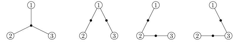
Figure 1. The trees in $\mathcal{G}_{0,3}$

3.4.2   $(g,n)=(1,1)$

We need to extract the coefficient of $\hbar^{1}$ in the formula of Theorem 3.5. Recall that the leading order was $\hbar^{-1}$, so this contribution may come from one of the three following possibilities:

• The vertex without hyperedges. Its weight is the coefficient of $\hbar^{1}$ in (24). If we pick the leading order $\varsigma(z)=1+O(z^{2})$ everywhere, we can get a contribution by picking one $G_{1,1}^{\vee}(w)$ in the last line. This comes without powers of $u$, so selects $r=0$; as $\varsigma$ was replaced by $1$, the exponential in the second line of (24) is $1$, thus forcing $m=0$. Another contribution comes from picking the second term $\frac{z^{2}}{24}$ from one occurrence of $\varsigma(z)$ and replacing the other occurrences of $\varsigma$ by $1$. If we pick this second term in $\varsigma$ from the denominator of the third line of (24), we will get a linear term in $u$, thus selecting $r=1$, while in the second line the exponential will be $1$, thus selecting $m=1$. If we rather pick it from the exponential in the third line, we get $u^{2}$, thus selecting $r=2$, while in the second line the exponential will be $1$, and as $(\partial_{y}+v/y)^{2}\cdot 1=(v^{2}-v)/y$, we get contributions from $m=1$ and $m=2$.

• The graph consisting of one white vertex connected in two ways to a black vertex (which admits $2$ automorphisms), with $\varsigma$ always replaced by $1$. In this case, we get $\vec{\mathsf{O}}_{r}^{\vee}(w)u^{2}G_{0,2}^{\vee}(w,w)$, which selects $r=1$ and subsequently $m=1$.

• The correction term $\Delta_{1}^{\vee}(X_{1})$ given by (27). We must select one term $\frac{z^{2}}{24}$ in $\varsigma(z)$ either from the numerator or the denominator in the exponential, hence get contributions from $m=0$ and $m=2$.

This results in:

$$\begin{split}G_{1,1}(X)&=P^{\vee}(w)G_{1,1}^{\vee}(w)-\frac{1}{24}P^{\vee}(w)w\partial_{w}\bigg{(}\frac{P^{\vee}(w)}{G_{0,1}^{\vee}(w)}\bigg{)}\\ &\quad+\frac{1}{24}P^{\vee}(w)w\partial_{w}(P^{\vee}(w)w\partial_{w}-1)\bigg{(}\frac{P^{\vee}(w)}{(G_{0,1}^{\vee}(w))^{2}}\,(w\partial_{w})^{2}G_{0,1}^{\vee}(w)\bigg{)}\\ &\quad+\frac{1}{2}P^{\vee}(w)w\partial_{w}\bigg{(}\frac{P^{\vee}(w)}{G_{0,1}^{\vee}(w)}\,G_{0,2}^{\vee}(w,w)\bigg{)}\\ &\quad-\frac{1}{24}\big{(}(P^{\vee}(w)w\partial_{w})^{2}-1\big{)}\frac{P^{\vee}(w)w\partial_{w}G^{\vee}_{0,1}(w)}{(G^{\vee}_{0,1}(w))^{2}}\,.\end{split}$$

After a tedious algebra, we observe many simplifications:

(33) $$\omega_{1,1}(x)+\omega_{1,1}^{\vee}(w)=\mathrm{d}\bigg{[}\frac{1}{2}\,\frac{\omega_{0,2}^{\vee}(w,w)}{\mathrm{d}x\,\mathrm{d}w}-\frac{1}{24}\,\frac{\mathrm{d}(\partial_{w}^{2}x/\partial_{w}x)}{\mathrm{d}x}\bigg{]}\,.$$

3.4.3   $(g,n)=(0,4)$

As shown in Figure 2, there are $29$ trees in $\mathcal{G}_{0,4}$, which can have $4$ different topologies once labellings are forgotten. The weight of a tree $T\in\mathcal{G}_{0,4}$ is given by $\mathcal{W}(T)\coloneqq\prod_{I\in\mathcal{I}(T)}^{\prime}G^{\vee}_{0,\#I}(w_{I})$, recalling that $\prod^{\prime}$ means that each occurrence of $G_{0,2}^{\vee}(w_{i},w_{j})$ for $i\neq j$ is replaced with $\widetilde{G}_{0,2}^{\vee}(w_{i},w_{j})$. Explicitly, the weight for each tree reads:

$$\begin{split}\mathcal{W}(T_{0})&=G^{\vee}_{0,4}(w_{1},w_{2},w_{3},w_{4})\,,\\ \mathcal{W}(T_{1}^{(i,j)})&=\widetilde{G}_{0,2}^{\vee}(w_{i},w_{j})\,G^{\vee}_{0,3}(w_{i},w_{k},w_{l})\,,\\ \mathcal{W}(T_{2}^{(i,j)})&=\widetilde{G}^{\vee}_{0,2}(w_{i},w_{j})\,\widetilde{G}^{\vee}_{0,2}(w_{i},w_{k})\,\widetilde{G}^{\vee}_{0,2}(w_{j},w_{l})\,,\\ \mathcal{W}(T_{3}^{(i)})&=\widetilde{G}^{\vee}_{0,2}(w_{i},w_{j})\,\widetilde{G}^{\vee}_{0,2}(w_{i},w_{k})\,\widetilde{G}^{\vee}_{0,2}(w_{i},w_{l})\,,\end{split}$$

where $\{i,j,k,l\}=[4]$.

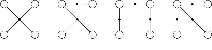
Figure 2. For $n=4$, there are $1+12+12+4$ trees in $\mathcal{G}_{0,4}$, which we call $T_{0}$, $T_{1}^{(i,j)}$, $T_{2}^{(i,j)}$ and $T_{3}^{(i)}$, respectively. In the two middle trees, $i,j\in[4]$ are pairwise distinct; in the last one $i\in[4]$. The missing indices ($k$ and $l$ for the two middle ones; $j,k$ and $l$ for the last one) are chosen so that $\{i,j,k,l\}=[4]$, and their order does not matter.

The functional relation of Theorem 3.10 for $n=4$ yields:

$$\begin{split}&G_{0,4}(X_{1},X_{2},X_{3},X_{4})=\bigg{(}\prod_{i=1}^{4}\vec{\mathsf{O}}_{0}^{\vee}(w_{i})\bigg{)}\mathcal{W}(T_{0})+\sum_{i=1}^{4}\vec{\mathsf{O}}_{1}^{\vee}(w_{i})\bigg{(}\prod_{\ell\neq i}\vec{\mathsf{O}}_{0}^{\vee}(w_{\ell})\bigg{)}\sum_{j\neq i}\mathcal{W}(T_{1}^{(i,j)})\\ &+\sum_{i=1}^{4}\vec{\mathsf{O}}_{1}^{\vee}(w_{i})\sum_{j\neq i}\vec{\mathsf{O}}_{1}^{\vee}(w_{j})\bigg{(}\prod_{\ell\neq i,j}\vec{\mathsf{O}}_{0}^{\vee}(w_{\ell})\bigg{)}\mathcal{W}(T_{2}^{(i,j)})+\sum_{i=1}^{4}\vec{\mathsf{O}}_{2}^{\vee}(w_{i})\bigg{(}\prod_{\ell\neq i}\vec{\mathsf{O}}_{0}^{\vee}(w_{\ell})\bigg{)}\mathcal{W}(T_{3}^{(i)})\\ &=\Big{(}\prod_{a=1}^{4}P^{\vee}(w_{a})\Big{)}\Bigg{[}\mathcal{W}(T_{0})-\sum_{i=1}^{4}w_{i}\partial_{w_{i}}\bigg{(}\frac{\sum_{j\neq i}\mathcal{W}(T_{1}^{(i,j)})}{G_{0,1}^{\vee}(w_{i})\frac{w_{i}}{x(w_{i})}\partial_{w_{i}}x(w_{i})}\bigg{)}\\ &+\sum_{i=1}^{4}\sum_{j\neq i}w_{i}w_{j}\partial_{w_{i}}\partial_{w_{j}}\bigg{(}\frac{\mathcal{W}(T_{2}^{(i,j)})}{G_{0,1}^{\vee}(w_{i})\frac{w_{i}}{x(w_{i})}\partial_{w_{i}}x(w_{i})G_{0,1}^{\vee}(w_{j})\frac{w_{j}}{x(w_{j})}\partial_{w_{j}}x(w_{j})}\bigg{)}\\ &+\sum_{i=1}^{4}w_{i}\partial_{w_{i}}\bigg{[}\frac{1}{\frac{w_{i}}{x(w_{i})}\partial_{w_{i}}x(w_{i})}w_{i}\partial_{w_{i}}+1\bigg{]}\bigg{(}\frac{\mathcal{W}(T_{3}^{(i)})}{(G_{0,1}^{\vee}(w_{i}))^{2}\frac{w_{i}}{x(w_{i})}\partial_{w_{i}}x(w_{i})}\bigg{)}\Bigg{]}\,,\end{split}$$

with the substitution $X_{a}=w_{a}/G_{0,1}^{\vee}(w_{a})=1/x_{a}$ for $a\in[4]$. In terms of the differential forms (28), the relation reads

$$\begin{split}\omega_{0,4}(x_{1},x_{2},x_{3},x_{4})&=\omega^{\vee}_{0,4}(x_{1},x_{2},x_{3},x_{4})-\sum_{i=1}^{4}\mathrm{d}_{w_{i}}\bigg{(}\frac{\sum_{j\neq i}\widetilde{\omega}_{0,2}^{\vee}(w_{i},w_{j})\,\omega_{0,3}^{\vee}(w_{i},w_{k},w_{l})}{\mathrm{d}x_{i}\,\mathrm{d}w_{i}}\bigg{)}\\ &+\sum_{i=1}^{4}\sum_{j\neq i}\mathrm{d}_{w_{i}}\mathrm{d}_{w_{j}}\bigg{(}\frac{\widetilde{\omega}_{0,2}^{\vee}(w_{i},w_{j})\,\widetilde{\omega}_{0,2}^{\vee}(w_{i},w_{k})\,\widetilde{\omega}_{0,2}^{\vee}(w_{j},w_{l})}{\mathrm{d}x_{i}\,\mathrm{d}w_{i}\,\mathrm{d}x_{j}\,\mathrm{d}w_{j}}\bigg{)}\\ &+\sum_{i=1}^{4}\mathrm{d}_{w_{i}}\bigg{(}\big{(}1+x_{i}\partial_{x_{i}}\big{)}\Big{(}\frac{\widetilde{\omega}_{0,2}^{\vee}(w_{i},w_{j})\,\widetilde{\omega}_{0,2}^{\vee}(w_{i},w_{k})\,\widetilde{\omega}_{0,2}^{\vee}(w_{i},w_{l})}{x_{i}\,\mathrm{d}x_{i}\,(\mathrm{d}w_{i})^{2}}\Big{)}\bigg{)},\end{split}$$

where we use the substitution $x_{a}=G_{0,1}^{\vee}(w_{a})/w_{a}$ for $a\in[4]$ and the convention for $i,j,k,l$ was explained in the legend of Figure 2.

3.5   Relation to topological recursion

When $G_{g,n}$ is the generating series of ordinary maps of genus $g$ with $n$ boundaries, $G_{g,n}^{\vee}$ enumerates fully simple maps of the same topology [BGF20, BCDGF19]. In this case, it is known since Eynard [Eyn04, Eyn11, Eyn16] that $\omega_{g,n}$s are computed by the topological recursion [EO07, EO09] applied to the spectral curve

$$\mathcal{S}=\big{(}\mathbb{P}^{1},x,w,\tfrac{\mathrm{d}z_{1}\mathrm{d}z_{2}}{(z_{1}-z_{2})^{2}}\big{)}\,,$$

while it was conjectured in [BGF20] and proved in [BDBKS23, BCGF21] that $\omega_{g,n}^{\vee}$s are computed by the topological recursion applied to

$$\mathcal{S}^{\vee}=\big{(}\mathbb{P}^{1},w,x,\tfrac{\mathrm{d}z_{1}\mathrm{d}z_{2}}{(z_{1}-z_{2})^{2}}\big{)}\,.$$

This gives a class of examples to test our functional relations numerically. The $(0,3)$ formula (32) was indeed shown to hold in this situation in [BGF20, Section 6], and here we see that in fact it holds in the greater generality provided by the master relation (5). To test the $(1,1)$ formula (33), let us consider the case of quadrangulations (maps with faces of degree $4$), which corresponds to the spectral curve in parametric form

$$x(z)=c\Big{(}z+\frac{1}{z}\Big{)}\,,\qquad w(z)=\frac{z^{2}-\tau}{cz^{3}}\,,\qquad\frac{\mathrm{d}z_{1}\mathrm{d}z_{2}}{(z_{1}-z_{2})^{2}}=\widetilde{\omega}_{0,2}(z_{1},z_{2})=\widetilde{\omega}_{0,2}^{\vee}(z_{1},z_{2})\,,$$

where $t$ is the weight per quadrangle, and

$$c=\sqrt{\frac{1-\sqrt{1-12t}}{6t}}\,,\qquad\tau=ct^{4}\,.$$

From this we deduce

$$\begin{split}\omega_{0,2}^{\vee}(z_{1},z_{2})&=\widetilde{\omega}_{0,2}^{\vee}(z_{1},z_{2})-\frac{w^{\prime}(z_{1})w^{\prime}(z_{2})\mathrm{d}z_{1}\mathrm{d}z_{2}}{(w(z_{1})-w(z_{2}))^{2}}=\frac{\tau\big{(}z_{1}^{2}z_{2}^{2}+\tau(z_{1}^{2}+4z_{1}z_{2}+z_{2}^{2})\big{)}\mathrm{d}z_{1}\mathrm{d}z_{2}}{\big{(}\tau(z_{1}^{2}+z_{1}z_{2}+z_{2}^{2})-z_{1}^{2}z_{2}^{2}\big{)}^{2}}\,,\\ \frac{\omega_{0,2}^{\vee}(z,z)}{2\,\mathrm{d}x(z)\,\mathrm{d}w(z)}&=-\frac{\tau z^{4}(z^{2}+6\tau)}{2(z^{2}-3\tau)^{3}(z^{2}-1)}\,,\end{split}$$

and

$$\begin{split}\frac{1}{24}\frac{\mathrm{d}}{\mathrm{d}x}\bigg{(}\frac{\partial_{w}^{2}x}{\partial_{w}x}\bigg{)}&=\frac{1}{24\,x^{\prime}(z)}\partial_{z}\bigg{(}\frac{1}{w^{\prime}(z)}\partial_{z}\ln\Big{(}\frac{x^{\prime}(z)}{w^{\prime}(z)}\Big{)}\bigg{)}\\ &=-\frac{z^{4}\big{(}z^{8}-3z^{6}(3\tau+1)+18\tau z^{4}(3\tau+1)+3\tau z^{2}(-33\tau+1)+27\tau^{2}\big{)}}{12(z^{2}-1)^{3}(z^{2}-3\tau)^{3}}\,.\end{split}$$

Besides, [BGF20, Section 5.2] computed from topological recursion:

(34) $$\begin{split}\omega_{1,1}(z)&=\frac{z\big{(}\tau z^{4}+z^{2}(1-5\tau)+\tau\big{)}}{(z^{2}-1)^{4}(3\tau-1)^{2}}\,\mathrm{d}z\,,\\ \omega_{1,1}^{\vee}(z)&=\frac{3\tau^{2}z\big{(}(3\tau-2)z^{4}+3\tau(9\tau-1)z^{2}-27\tau^{3}\big{)}}{(z^{2}-3\tau)^{4}(3\tau-1)^{2}}\,\mathrm{d}z\,,\end{split}$$

and we checked that (33) is indeed satisfied.

We suggest that the master relation (5), or rather the functional relations given in Theorem 3.5 when written in terms of differentials, in fact describe the effect of the symplectic exchange $x\leftrightarrow w$ in topological recursion.

Conjecture 3.14.

Let $\mathcal{C}$ be a compact Riemann surface, $x,w$ are meromorphic functions on $\mathcal{C}$ such that $\mathrm{d}x$ and $\mathrm{d}w$ do not have common zeroes, and $\mathcal{B}$ is a fundamental bidifferential of the second kind. We call $\omega_{g,n}$ the differentials obtained from the topological recursion with the spectral curve $(\mathcal{C},x,w,\mathcal{B})$, and $\omega_{g,n}^{\vee}$ the ones associated to the spectral curve $(\mathcal{C},w,x,\mathcal{B})$, and define $\widetilde{\omega}_{0,2}=\widetilde{\omega}_{0,2}^{\vee}=\mathcal{B}$. Then, these differentials will satisfy for all $2g-2+n\geq 0$ the functional relations of Theorem 3.5 (after they are converted in relations between meromorphic differentials on $\mathcal{C}$).

This conjecture holds by definition for $(g,n)=(0,2)$. It holds for $(0,3)$ (formula justified in [BGF20]) as well as for $(1,1)$ by comparison of (33) with [EO07, Lemma C.1] where one can use $w$ as a coordinate. Besides, as we have just discussed, it holds for all $(g,n)$ in the case of spectral curves corresponding to map enumeration. This conjecture should be a step towards understanding the symplectic invariance property of topological recursion envisioned in [EO08, EO13], which one should extract from the analytic properties of $\omega_{g,1}+\omega_{g,1}^{\vee}$ for all $g\geq 1$.

Furthermore, the conjecture remains true in the more general context of the matrix model with external field. The generalised resolvents of the matrix model with external field were proved to satisfy topological recursion in [EO07, EO09], while the topological recursion for the same spectral curve, but after exchanging the role of $x$ and $w$, produces diagonal correlation functions of the matrix model with external field [BCEGF21, Section 4.1], which combinatorially corresponds to the enumeration of the so-called ciliated maps. As proved in [BGF20] and recalled in Theorem 5.26, the master relation appears in general unitarily invariant ensembles of random hermitian matrices, so it also applies to the generalised resolvents (of the type $p_{\lambda}$ in Theorem 5.26) and the diagonal correlation functions (of the type $\mathcal{P}_{\nu}$ in Theorem 5.26) of the matrix model with external field.

3.6   Analytic properties

Whether the generating series are Taylor expansions of analytic functions depends on the topological partition functions that one starts with. However, we can deduce from Theorem 3.5 that the master transformation induced by $\mathsf{D}$ respects the analytic properties of the generating functions, provided one understands well the analytic properties for the $(0,1)$-case.

Proposition 3.15.

Let $Z,Z^{\vee}$ be two topological partition functions such that $Z=\mathsf{D}Z^{\vee}$, and $G_{g,n},G_{g,n}^{\vee}$ the generating series coming from the topological expansion of their $n$-point functions, cf. Section 3.1. Suppose that there exists a Riemann surface $\Sigma$ equipped with a marked point $q_{\infty}$ and two meromorphic functions $\mathsf{x}$ and $\mathsf{w}$ such that

• $q_{\infty}$ is a simple pole of $\mathsf{x}$ and a simple zero of $\mathsf{w}$;

• $W_{0,1}\circ\mathsf{x}$ is the series expansion of the function $\mathsf{w}$ near $q_{\infty}$, and $X_{0,1}\circ\mathsf{w}$ is the series expansion of the function $\mathsf{x}$ near $q_{\infty}$.

Then, the two properties are equivalent:

• for $2g-2+n\geq 0$, $G_{g,n}(1/\mathsf{x}(z_{1}),\ldots,1/\mathsf{x}(z_{n}))$ is the series expansion of a meromorphic function of $(z_{1},\ldots,z_{n})\in\Sigma^{n}$ near $(q_{\infty},\ldots,q_{\infty})$;

• for $2g-2+n\geq 0$, $G_{g,n}^{\vee}(\mathsf{w}(z_{1}),\ldots,\mathsf{w}(z_{n}))$ is the series expansion of a meromorphic function of $(z_{1},\ldots,z_{n})\in\Sigma^{n}$ near $(q_{\infty},\ldots,q_{\infty})$.

Proof.

Assume (ii). We first observe that $\frac{1}{\mathsf{x}}$ gives a meromorphic analytic continuation on $\Sigma$ of $X\circ\mathsf{w}$, and $\frac{\mathsf{x}\mathrm{d}\mathsf{w}}{\mathsf{w}\mathrm{d}\mathsf{x}}$ gives a meromorphic analytic continuation on $\Sigma$ of $P^{\vee}\circ\mathsf{w}$.

Second, $G_{0,2}(1/\mathsf{x}(z_{1}),1/\mathsf{x}(z_{2}))$ admits an analytic continuation as a meromorphic function of $(z_{1},z_{2})\in\Sigma^{2}$ because the right-hand side of (25) manifestly does. As $\widetilde{G}_{0,2}(1/\mathsf{x}(z_{1}),1/\mathsf{x}(z_{2}))$ is obtained from $G_{0,2}$ by the addition of a manifestly meromorphic term (cf. (21)), it also admits an analytic continuation as a meromorphic function of $(z_{1},z_{2})\in\Sigma^{2}$.

Third, for any fixed $g\geq 1$, the right-hand side of (27) contains only a finite sum over $m$, consisting of operators that are polynomial in $G_{0,1}^{\vee}(w)$, in $P^{\vee}(w)$, in $w$, in $\partial_{w}$ and in $\partial_{G_{0,1}^{\vee}(w)}$, acting on $P^{\vee}(w)w\partial_{w}G_{0,1}^{\vee}(w)$. The derivations $\partial_{w}(\cdot)$ and $\partial_{G_{0,1}^{\vee}(w)}(\cdot)$ acting on formal power series of $w$ correspond at the level of meromorphic functions on $\Sigma$ to the operations $\frac{1}{\mathrm{d}\mathsf{w}}\mathrm{d}(\cdot)$ and $\frac{1}{\mathrm{d}(\mathsf{x}\mathsf{w})}\mathrm{d}(\cdot)$. We deduce that $\Delta_{g}^{\vee}(1/\mathsf{x}(z))$ admits an analytic continuation as a meromorphic function of $z\in\Sigma$.

Last, for fixed $(g,n)$ with $2g-2+n>0$, $G_{g,n}$ is expressed in terms of $G^{\vee}_{g^{\prime},n^{\prime}}$ via (26), involving the term $\Delta_{g}^{\vee}$ that we just handled (present for $n=1$ only) and a sum over graphs from Definition 3.2. Only the finitely many graphs with first Betti number bounded by $g$ can contribute. The weight of these graphs is described in Definition 3.4. As $G_{g,n}$ appears as the coefficient of $\hbar^{2g-2+n}$ in the weighted sum, the formal series $\varsigma$ (cf. (23)) appearing in the weight of hyperedges $\mathsf{c}^{\vee}$ and in the operator $\vec{\mathsf{O}}$ for white vertices can effectively be truncated to a polynomial of some degree depending on $g$ and $n$. So, the weight of a hyperedge of cardinality $\#I$ can be replaced by a truncated weight admitting a meromorphic analytic continuation in $\Sigma^{\#I}$. Likewise, in the truncation of the operator-valued weight of white vertices, the sum over $r,m$ (see (24)) only receives finitely many contributions:

• the sum over $r$ is associated to the coefficient of $u_{i}^{r}$. This variable appears to be multiplied by $\hbar$ in the expressions of $\mathsf{c}^{\vee}$ and $\vec{\mathsf{O}}$. Since we extract the coefficient of $\hbar^{2g-2+n}$ in the weighted sum, $r$ is bounded by $2g-2+n$.

• The sum over $m$ is associated to the coefficient of $v_{i}^{m}$. Since the sum over $r$ is bounded and we extract the coefficient of $\hbar^{2g-2+n}$, the expression for $\vec{\mathsf{O}}$ is actually a polynomial in $v_{i}$. Therefore the sum over $m$ is finite.

Those contributions are polynomials in generating series and derivations that admit meromorphic analytic continuation on $\Sigma$. Therefore, $G_{g,n}(1/\mathsf{x}(z_{1}),\ldots,1/\mathsf{x}(z_{n}))$ admits an analytic continuation as a meromorphic function of $(z_{1},\ldots,z_{n})\in\Sigma^{n}$, and we have checked (i).

The proof of (i) $\Rightarrow$ (ii) is completely analogous based on the dual expressions of $G_{g,n}^{\vee}$ in terms of $G_{g,n}$ given in Section 4.3. ∎

The assumption on analytic properties of $(0,1)$ in Proposition 3.15 could be reformulated as: $G_{0,1}(1/\mathsf{x}(z))$ and $G_{0,1}^{\vee}(\mathsf{w}(z))$ both represent the series expansion of the function $\mathsf{x}(z)\mathsf{w}(z)$ of $z\in\Sigma$ near $q_{\infty}$. The triple $(\Sigma,\mathsf{x},\mathsf{w})$ is then called spectral curve. In full generality checking whether there exists or not a spectral curve (and constructing it explicitly enough) is hard, but it can be handled in specific examples, in particular when $W_{0,1}$ is the series expansion of an algebraic function (as in the example of Section 3.5).

The conclusion of Proposition 3.15 could be reformulated using the differential form-valued generating series: the $\omega_{g,n}$ extend to meromorphic $n$-forms on $\Sigma^{n}$ for $2g-2+n\geq 0$ if and only if $\omega_{g,n}^{\vee}$ do. If this is the case, we usually keep using the symbols $\omega_{g,n}$ and $\omega_{g,n}^{\vee}$ for these meromorphic $n$-forms on $\Sigma^{n}$. In these terms, for instance, (31) translates into an identity between meromorphic bidifferentials on $\Sigma^{2}$

$$\omega_{0,2}+\frac{\mathrm{d}\mathsf{x}_{1}\mathrm{d}\mathsf{x}_{2}}{(\mathsf{x}_{1}-\mathsf{x}_{2})^{2}}=\omega_{0,2}^{\vee}+\frac{\mathrm{d}\mathsf{w}_{1}\mathrm{d}\mathsf{w}_{2}}{(\mathsf{w}_{1}-\mathsf{w}_{2})^{2}}\,,$$

where $\mathsf{x}_{i}=\mathsf{x}\circ{\rm pr}_{i}$ and ${\rm pr}_{i}:\Sigma^{2}\rightarrow\Sigma$ is the projection on the $i$-th copy. Likewise, (33) translates into an identity of meromorphic $1$-forms on $\Sigma$

(35) $$\mathsf{\omega}_{1,1}+\omega_{1,1}^{\vee}=\mathrm{d}\Bigg{[}\frac{\iota^{*}\omega_{0,2}^{\vee}}{2\,\mathrm{d}\mathsf{x}\,\mathrm{d}\mathsf{w}}-\frac{1}{24\,\mathrm{d}\mathsf{x}}\mathrm{d}\Big{(}\frac{\mathrm{d}\big{(}\frac{\mathrm{d}\mathsf{x}}{\mathrm{d}\mathsf{w}}\big{)}}{\mathrm{d}\mathsf{x}}\Big{)}\bigg{]}\,,$$

where $\iota:\Sigma\rightarrow\Sigma\times\Sigma$ is the diagonal inclusion (specialisation to the two same points).

As the formula in Theorem 3.5 has an explicit structure, the location and order of poles of $\omega_{g,n}^{\vee}$ knowing the singularities of $\omega_{g,n}$ (or vice versa) could in principle be described, but we do not pursue it here.

4   Proof of the main results

4.1   All genus: proof of Theorem 3.5

We rely on the description of the projective representation of $\widehat{\mathfrak{gl}}_{\infty}(R)$ in terms of differential operators on $\mathcal{F}_{R}$ [Kac90]. Our starting point is the formula found e.g. in [BDBKS22, Proposition 3.1], expressing the conjugation of the Heisenberg field with the operator $\mathsf{D}$ or $\mathsf{D}^{-1}$:

(36) $$\begin{split}\mathsf{D}^{\mp 1}\,\widetilde{\mathsf{J}}(X)\,\mathsf{D}^{\pm 1}&=\sum_{k\in\mathbb{Z}}X^{k}[w^{k}]\,\,\sum_{r\geq 0}\partial_{y}^{r}\exp\bigg{(}\pm k\,\frac{\varsigma(k\hbar\partial_{y})}{\varsigma(\hbar\partial_{y})}\ln(1+y)\bigg{)}\Big{|}_{y=0}[u^{r}]\frac{1}{\hbar u\varsigma(\hbar u)}\\ &\quad\cdot\exp\bigg{(}\sum_{m>0}\hbar u\,\varsigma(\hbar uw\partial_{w})\mathsf{J}_{-m}w^{-m}\bigg{)}\exp\bigg{(}\sum_{m>0}\hbar u\,\varsigma(\hbar uw\partial_{w})\mathsf{J}_{m}w^{m}\bigg{)}\,,\end{split}$$

where we recall $\varsigma(w)=2w^{-1}{\rm sinh}(w/2)=1+\frac{w^{2}}{24}+O(w^{4})$. Let us employ this formula with the sign $+$, substitute it in Equation (20) and then make use of the commutation relations $[\mathsf{J}_{l},\mathsf{J}_{m}]=l\delta_{l+m,0}$, as well as the properties $\langle|\mathsf{J}_{-m}=0$ and $\mathsf{J}_{m}|\rangle=0$, for $m>0$. As explained in [BDBKS23, Section 2] (the case discussed in op. cit. is a bit more general: it depends on a choice of a formal power series $\psi(y,\hbar^{2})$ that is equal to $\log(1+y)$ in our case), we obtain a sum over the graphs of Definition 3.2, where the weights consist of the following elementary blocks.

Definition 4.1.

We fix variables $(u_{i},v_{i},w_{i})_{i=1}^{n}$.

• To a hyperedge $I\subseteq[n]$, we attach the weight (already in Definition 3.4):

  $$\mathsf{c}^{\vee}(u_{I},w_{I})=\prod_{i\in I}\hbar u_{i}\varsigma(\hbar u_{i}w_{i}\partial_{w_{i}})\widetilde{G}^{\vee}_{\#I}(w_{I})\,.$$

• To the $i$-th white vertex, we attach the operator weight:

  (37) $$\begin{split}\vec{\mathsf{U}}^{\vee}(X_{i})&=\sum_{k\in\mathbb{Z}}X_{i}^{k}\cdot[w_{i}^{k}]\,\,\sum_{r\geq 0}\partial_{y}^{r}\exp\bigg{(}k\,\frac{\varsigma(k\hbar\partial_{y})}{\varsigma(\hbar\partial_{y})}\,\ln(1+y)\bigg{)}\Big{|}_{y=0}\\ &\phantom{\sum_{k\in\mathbb{Z}}X_{i}^{k}}\!\!\cdot[u_{i}^{r}]\,\,\frac{\exp\big{(}\hbar u_{i}\,\varsigma(\hbar u_{i}w_{i}\partial_{w_{i}})(G_{1}^{\vee}(w_{i})-\hbar^{-1})\big{)}}{\hbar u_{i}\,\varsigma(\hbar u_{i})}\,.\end{split}$$

This operator acts from the left on series depending on variables $u_{i}$ and $w_{i}$ and gives as output a series in $X_{i}$. The subtraction of $\hbar^{-1}$ in the last line kills the conventional constant added in the definition of the $1$-point function in (21).

Lemma 4.2 (Key combinatorial identity).

The relation $Z=\mathsf{D}Z^{\vee}$ is equivalent to the relations:

(38) $$\forall n>0,\qquad\widetilde{G}_{n}(X_{1},\ldots,X_{n})=\sum_{\Gamma\in\mathcal{G}_{n}}\frac{1}{\#{\rm Aut}(\Gamma)}\prod_{i=1}^{n}\vec{\mathsf{U}}^{\vee}(X_{i})\prod_{I\in\mathcal{I}(\Gamma)}\mathsf{c}^{\vee}(u_{I},w_{I})\,,$$

where the first product is taken from left to right with $i$ increasing.

Proof.

For the proof we just give a dictionary that explains how to match Equation (38) to the statement of [BDBKS23, Lemma 2.1] assuming that the function $\psi(y,\hbar^{2})$ in op. cit. is set to be $\ln(1+y)$, and the variables $z_{i}$ there correspond to $w_{i}$ in our notation. In order to follow the table below one needs to remember the notation and terminology used in [BDBKS23, Lemma 2.1].

Graphs in equation (38)	Graphs in [BDBKS23, Lemma 2.1]
$\bullet\;$ the white vertex labeled by $i$ ($i=1,\ldots n$)	$\bullet\;$ the white vertex labeled by $i$, ($i=1,\ldots n$)
$\bullet\;$ a hyperedge of cardinality $\geq 3$	$\bullet\;$ a multi-edge of cardinality $\geq 3$
$\bullet\;$ a hyperedge of cardinality $2$ incident to	$\bullet\;$ the formal sum of a multi-edge of cardinality
two different white vertices labeled by $i$ and $j$	$2$ incident to two different white vertices labeled
	by $i$ and $j$ and an ordinary edge connecting
	these two vertices
$\bullet\;$ a hyperedge of cardinality $2$ incident	$\bullet\;$ a multi-edge of cardinality $2$ incident (twice)
(twice) to the white vertex labeled by $i$	to the white vertex labeled by $i$
$\bullet\;$ the extra factor for the white vertex labeled	$\;\bullet\;$ the union of all multi-edges of cardinality $1$
by $i$ (the numerator of the second line in (37))	incident to the white vertex labeled by $i$

With this dictionary, we see that the contribution of all multi-edges of cardinality $\geq 3$ is exactly the same in both formulas; one just has to identify the expansions of $G_{k}^{\vee}(w_{1},\dots,w_{k})$ with $s_{g;t_{1},\dots,t_{k}}$ in [BDBKS23, Equation (11)]. The same holds for hyperedges (in our terminology) of cardinality two that are incident twice to the same white vertex.

Consider a hyperedge of cardinality $2$ incident to two different white vertices labeled by $i$ and $j$. By our convention, we assign to it the weight

$$\big{(}\hbar u_{i}\,\varsigma(\hbar u_{i}w_{i}\partial_{w_{i}})\big{)}\big{(}\hbar u_{j}\,\varsigma(\hbar u_{j}w_{j}\partial_{w_{j}})\big{)}\bigg{(}\,G_{2}^{\vee}(w_{i},w_{j})+\frac{w_{i}w_{j}}{(w_{i}-w_{j})^{2}}\bigg{)}\,.$$

It is possible to say that for each such hyperedge we can choose either the first summand or the second one, and to take the sum over all possible choices for all such edges. In the notation and terminology of [BDBKS23, Lemma 2.1] the first choice is the weight associated to the respective multi-edge, and the second choice is the weight associated to what is called an ordinary edge in op. cit.

In the notation of [BDBKS23, Lemma 2.1], there can be any non-negative number of multi-edges of cardinality $1$ attached to a white vertex labeled by $i$. Taking into account the total weight is equal to the inverse order of the automorphisms of the graph, the weights of all such edges can be assembled into the extra exponential factors. These exponential factors are, in our notation, precisely $\exp\big{(}\hbar u_{i}\,\varsigma(\hbar u_{i}w_{i}\partial_{w_{i}})(G_{1}^{\vee}(w_{i})-\hbar^{-1})\big{)}$ for each $i=1,\dots,n$ (the shift by $\hbar^{-1}$ is the result of the convention we have chosen in Equation (21)). Note that these factors are exactly the missing ones that we need to match our operators $\vec{\mathsf{U}}^{\vee}(X_{i})$ and the corresponding operators in [BDBKS23, Lemma 2.1].

This completes the comparison and establishes (38) as a special case of [BDBKS23, Lemma 2.1]. ∎

To pass from (38) to the statement of Theorem 3.5, in particular to (26), we proceed in three steps, which were suggested by Kazarian in an unpublished manuscript (see [Kaz19, Kaz20]). In our exposition we follow [BDBKS22, Section 4.4].

First, if $\Phi(y)$, $\Psi(u)$ and $Y(w)$ are three formal power series with $Y(w)=O(w)$, we observe that

(39) $$\sum_{r\geq 0}(\partial_{y}^{r}\Phi)(0)\cdot[u^{r}]\,\,e^{uY(w)}\Psi(u)=\sum_{r\geq 0}(\partial_{y}^{r}\Phi)(Y(w))\cdot[u^{r}]\,\,\Psi(u)\,,$$

which can be checked by direct expansion of the left-hand side in the variable $w$. This observation applied to $Y(w_{i})=G_{0,1}^{\vee}(w_{i})-1$ allows us to remove the otherwise infinitely many contributions $\exp\big{(}u_{i}(G^{\vee}_{0,1}(w_{i})-1)\big{)}$ in the second line of (37). Note that this second line of (37) starts with $1/u$ for $n=1$. We will discuss this case separately later. For $n\geq 2$, Equation (38) is turned by this trick into

(40) $$\begin{split}&\widetilde{G}_{n}(X_{1},\ldots,X_{n})\\ &=\prod_{i=1}^{n}\Bigg{[}\sum_{k\in\mathbb{Z}}X_{i}^{k}\cdot[w_{i}^{k}]\,\,\sum_{r\geq 0}\partial_{y}^{r}\exp\bigg{(}k\,\frac{\varsigma(k\hbar\partial_{y})}{\varsigma(\hbar\partial_{y})}\,\ln(1+y)\bigg{)}\Big{|}_{y=G^{\vee}_{0,1}(w_{i})-1}[u_{i}^{r}]\\ &\quad\frac{\exp\big{(}\hbar u_{i}\,\varsigma(\hbar u_{i}w_{i}\partial_{w_{i}})(G_{1}^{\vee}(w_{i})-\hbar^{-1})-u_{i}(G_{0,1}^{\vee}(w_{i})-1)\big{)}}{\hbar u_{i}\,\varsigma(\hbar u_{i})}\Bigg{]}\sum_{\Gamma\in\mathcal{G}_{n}}\frac{\prod_{I\in\mathcal{I}(\Gamma)}\mathsf{c}^{\vee}(u_{I},w_{I})}{\#{\rm Aut}(\Gamma)}\,.\end{split}$$

Second, we have to remove the explicit dependence on $k$s coming from the weight of the white vertices (37). To this end, we use for $r\geq 0$ and $k\in\mathbb{Z}$:

(41) $$\begin{split}&\partial_{y}^{r}\exp\Big{(}k\frac{\varsigma(k\hbar\partial_{y})}{\varsigma(\hbar\partial_{y})}\ln(1+y)\Big{)}\Big{|}_{y=G^{\vee}_{0,1}(w)-1}=\partial_{y}^{r}\exp\Big{(}k\frac{\varsigma(k\hbar\partial_{y})}{\varsigma(\hbar\partial_{y})}\ln y\Big{)}\Big{|}_{y=G^{\vee}_{0,1}(w)}\\ &=(G^{\vee}_{0,1}(w))^{k}\cdot\bigg{(}\exp(-k\ln y)\partial_{y}^{r}\exp\Big{(}k\frac{\varsigma(k\hbar\partial_{y})}{\varsigma(\hbar\partial_{y})}\ln y\Big{)}\bigg{)}\Big{|}_{y=G^{\vee}_{0,1}(w)}\\ &=(G^{\vee}_{0,1}(w))^{k}\cdot\bigg{(}\Big{(}\partial_{y}+\frac{k}{y}\Big{)}^{r}\exp\Big{(}k\big{(}\frac{\varsigma(k\hbar\partial_{y})}{\varsigma(\hbar\partial_{y})}-1\big{)}\ln y\Big{)}\bigg{)}\Big{|}_{y=G^{\vee}_{0,1}(w)}\,.\end{split}$$

The second factor here has a polynomial dependence on $k$ in each degree in $\hbar$, and we can use the following trick to assemble it: if $Q(k)$ is a polynomial in $k$, we have

$$\sum_{k}Q(k)\,X^{k}=Q(X\partial_{X})\sum_{k}X^{k}=\sum_{j\geq 0}(X\partial_{X})^{j}\,[v^{j}]\,\sum_{k}X^{k}Q(v)\,.$$

For every given monomial in $\hbar,X_{1},\ldots,X_{n}$, we need to use such a formula when the summation ranges over a set of integers $k$ bounded from below, in which case it makes sense in the framework explained in Remark 3.1. Equation (40) is turned by this trick into

(42) $$\begin{split}&\widetilde{G}_{n}(X_{1},\ldots,X_{n})=\prod_{i=1}^{n}\Bigg{[}\sum_{j=0}^{\infty}(X_{i}\partial_{X_{i}})^{j}[v^{j}]\sum_{k\in\mathbb{Z}}X_{i}^{k}\cdot[w_{i}^{k}](G^{\vee}_{0,1}(w_{i}))^{k}\cdot\\ &\quad\sum_{r\geq 0}\bigg{(}\Big{(}\partial_{y}+\frac{v}{y}\Big{)}^{r}\exp\Big{(}v\big{(}\frac{\varsigma(v\hbar\partial_{y})}{\varsigma(\hbar\partial_{y})}-1\big{)}\ln y\Big{)}\bigg{)}\Big{|}_{y=G^{\vee}_{0,1}(w_{i})}[u_{i}^{r}]\\ &\quad\frac{\exp\big{(}\hbar u_{i}\,\varsigma(\hbar u_{i}w_{i}\partial_{w_{i}})(G_{1}^{\vee}(w_{i})-\hbar^{-1})-u_{i}(G_{0,1}^{\vee}(w_{i})-1)\big{)}}{\hbar u_{i}\,\varsigma(\hbar u_{i})}\Bigg{]}\sum_{\Gamma\in\mathcal{G}_{n}}\frac{\prod_{I\in\mathcal{I}(\Gamma)}\mathsf{c}^{\vee}(u_{I},w_{I})}{\#{\rm Aut}(\Gamma)}\,.\end{split}$$

Third, to remove the factor of $(G^{\vee}_{0,1}(w_{i}))^{k}$ in (42), we use the Lagrange inversion formula: given a Laurent series $L(w)$, we have for any $k\in\mathbb{Z}$,

(43) $$\sum_{k\in\mathbb{Z}}X^{k}\cdot[\tilde{w}^{k}]\,\,(G^{\vee}_{0,1}(\tilde{w}))^{k}L(\tilde{w})=\frac{\mathrm{d}\ln w}{\mathrm{d}\ln X}\,L(w)\,,\qquad{\rm where}\;\;X=\frac{w}{G^{\vee}_{0,1}(w)}\,.$$

Using this observation for each $i\in[n]$, we obtain for $n\geq 2$ and $g\geq 0$:

(44) $$\widetilde{G}_{g,n}(X_{1},\ldots,X_{n})=[\hbar^{2g-2+n}]\,\,\sum_{\Gamma\in\mathcal{G}_{n}}\frac{1}{\#{\rm Aut}(\Gamma)}\prod_{i=1}^{n}\vec{\mathsf{O}}^{\vee}(w_{i})\prod_{I\in\mathcal{I}(\Gamma)}\mathsf{c}^{\vee}(u_{I},w_{I})\,,$$

using the substitutions

(45) $$X_{i}=\frac{w_{i}}{G_{0,1}^{\vee}(w_{i})}\,,\qquad P^{\vee}(w_{i})=\frac{\mathrm{d}\ln w_{i}}{\mathrm{d}\ln X_{i}}\,,\qquad X_{i}\partial_{X_{i}}=P^{\vee}(w_{i})w_{i}\partial_{w_{i}}\,.$$

The operators $\vec{\mathsf{O}}^{\vee}(X_{i})$ are those introduced in (24), and they involve the above choice of $P^{\vee}(w_{i})$. For $2g-2+n>0$, the left-hand side is simply $G_{g,n}(X_{1},\ldots,X_{n})$ and we recover (26). Up to the comparison of the right-hand side in the case $(g,n)=(0,2)$ to the second formula of (25) and the study of the special case $(g,n)=(0,1)$, which will both be carried out in the next section, this concludes the proof of Theorem 3.5 for $n\geq 2$.

In the case $n=1$ we have to make one more extra step. There is a graph that contains just one vertex and no hyperedges. The expression that we assign to this graph by Definition 4.1 is equal to the operator (37) applied to the constant $1$. Then, in order to apply Equation (39), we have to remove manually the singularity in $u$ as it is done in [BDBKS22, Section 6.2], that is, we have:

$$\begin{split}&\quad G_{1}(X)-\hbar^{-1}\\ &=\sum_{k\geq 1}X^{k}\cdot[w^{k}]\,\,\sum_{r\geq 0}\partial_{y}^{r}\exp\bigg{(}k\,\frac{\varsigma(k\hbar\partial_{y})}{\varsigma(\hbar\partial_{y})}\,\ln(1+y)\bigg{)}\Big{|}_{y=0}\\ &\phantom{=\sum_{k\geq 1}X^{k}}\,\,\cdot[u^{r}]\,\,\Bigg{(}\frac{\exp\big{(}\hbar u\,\varsigma(\hbar uw\partial_{w})(G_{1}^{\vee}(w)-\hbar^{-1})\big{)}}{\hbar u\,\varsigma(\hbar u)}-\frac{\exp\big{(}u(G^{\vee}_{0,1}(w)-1)\big{)}}{\hbar u}\Bigg{)}\\ &\quad+\sum_{k\geq 1}X^{k}\cdot[w^{k}]\,\,\sum_{r\geq 0}\partial_{y}^{r}\exp\bigg{(}k\,\frac{\varsigma(k\hbar\partial_{y})}{\varsigma(\hbar\partial_{y})}\,\ln(1+y)\bigg{)}\Big{|}_{y=0}\cdot[u^{r}]\,\,\frac{\exp\big{(}u\,(G^{\vee}_{0,1}(w)-1)\big{)}}{\hbar u}\,.\end{split}$$

The first summand here can be evaluated by the three steps performed above in the general case, and it gives the contribution of the graph with one vertex and no edges in the statement of Theorem 3.5. Let us show that the second summand is equal to $G_{0,1}(w)-\hbar^{-1}+\sum_{g\geq 1}\hbar^{2g-1}\Delta_{g}^{\vee}(X)$. We follow the computation done in [BDBKS22, Section 6.2], and this computation just implements the same three steps as above with an extra small step to remove the singularity in $u$ and further simplifications related to the specifics of this simpler formula:

(46) $$\begin{split}&\sum_{k\geq 1}X^{k}\cdot[w^{k}]\,\,\sum_{r\geq 0}\partial_{y}^{r}\exp\bigg{(}k\,\frac{\varsigma(k\hbar\partial_{y})}{\varsigma(\hbar\partial_{y})}\,\ln(1+y)\bigg{)}\Big{|}_{y=0}\cdot[u^{r}]\,\,\frac{\exp\big{(}u\,(G^{\vee}_{0,1}(w)-1)\big{)}}{\hbar u}\\ &=\int_{0}^{X}\frac{dX}{X}\sum_{k\geq 1}X^{k}\cdot[w^{k}]\,\,\sum_{r\geq 0}\partial_{y}^{r}\exp\bigg{(}k\,\frac{\varsigma(k\hbar\partial_{y})}{\varsigma(\hbar\partial_{y})}\,\ln(1+y)\bigg{)}\Big{|}_{y=0}\cdot[u^{r}]\,\,w\partial_{w}\frac{\exp\big{(}u\,(G^{\vee}_{0,1}(w)-1)\big{)}}{\hbar u}\\ &=\int_{0}^{X}\frac{dX}{X}\sum_{k\geq 1}X^{k}\cdot[w^{k}]\,\,\sum_{r\geq 0}\partial_{y}^{r}\exp\bigg{(}k\,\frac{\varsigma(k\hbar\partial_{y})}{\varsigma(\hbar\partial_{y})}\,\ln(1+y)\bigg{)}\Big{|}_{y=0}\cdot[u^{r}]\,\,\frac{\exp\big{(}u\,(G^{\vee}_{0,1}(w)-1)\big{)}}{\hbar}w\partial_{w}G^{\vee}_{0,1}(w)\\ &=\int_{0}^{X}\frac{dX}{X}\sum_{k\geq 1}X^{k}\cdot[w^{k}]\,\,\sum_{r\geq 0}\partial_{y}^{r}\exp\bigg{(}k\,\frac{\varsigma(k\hbar\partial_{y})}{\varsigma(\hbar\partial_{y})}\,\ln y\bigg{)}\Big{|}_{y=G^{\vee}_{0,1}(w)}\cdot[u^{r}]\,\,\frac{w\partial_{w}G^{\vee}_{0,1}(w)}{\hbar}\,.\end{split}$$

Since the last factor of this expression does not depend on $u$, we continue the computation substituting $r=0$:

$$\begin{split}\eqref{eq:TowardsDelta}&=\int_{0}^{X}\frac{dX}{X}\sum_{k\geq 1}X^{k}\cdot[w^{k}]\exp\bigg{(}k\,\frac{\varsigma(k\hbar\partial_{y})}{\varsigma(\hbar\partial_{y})}\,\ln y\bigg{)}\Big{|}_{y=G^{\vee}_{0,1}(w)}\frac{w\partial_{w}G^{\vee}_{0,1}(w)}{\hbar}\\ &=\int_{0}^{X}\frac{dX}{X}\sum_{j=0}^{\infty}(X\partial_{X})^{j}\cdot[v^{j}]\sum_{k\geq 1}X^{k}\cdot[w^{k}](G^{\vee}_{0,1}(w))^{k}\\ &\quad\cdot\exp\bigg{(}v\,\frac{\varsigma(v\hbar\partial_{y})}{\varsigma(\hbar\partial_{y})}\,\ln y-v\ln y\bigg{)}\Big{|}_{y=G^{\vee}_{0,1}(w)}\frac{w\partial_{w}G^{\vee}_{0,1}(w)}{\hbar}\\ \end{split}$$

$$\begin{split}&=\frac{1}{\hbar}\int_{0}^{X}\frac{dX}{X}\sum_{j=0}^{\infty}(X\partial_{X})^{j}[v^{j}]\exp\bigg{(}v\,\frac{\varsigma(v\hbar\partial_{y})}{\varsigma(\hbar\partial_{y})}\,\ln y-v\ln y\bigg{)}\Big{|}_{y=G^{\vee}_{0,1}(w)}\frac{1}{P^{\vee}(w)}w\partial_{w}G^{\vee}_{0,1}(w)\\ &=\frac{1}{\hbar}\int_{0}^{X}\frac{dX}{X}\sum_{j=1}^{\infty}(X\partial_{X})^{j}[v^{j}]\exp\bigg{(}v\,\frac{\varsigma(v\hbar\partial_{y})}{\varsigma(\hbar\partial_{y})}\,\ln y-v\ln y\bigg{)}\Big{|}_{y=G^{\vee}_{0,1}(w)}\frac{1}{P^{\vee}(w)}w\partial_{w}G^{\vee}_{0,1}(w)\\ &\quad+\frac{1}{\hbar}\int_{0}^{X}\frac{dX}{X}\frac{1}{P^{\vee}(w)}w\partial_{w}G^{\vee}_{0,1}(w)\,.\end{split}$$

Having written it this way, we can directly integrate (recall that $P^{\vee}(w)w\partial_{w}=X\partial_{X}$). The result of the integration of the first summand is manifestly $\sum_{g=1}^{\infty}\hbar^{2g-1}\Delta^{\vee}_{g}(X)$ and the integration of the second term gives $\hbar^{-1}(G^{\vee}_{0,1}(w)-1)$, with $X=w/G^{\vee}_{0,1}(w)$. This completes the proof of Theorem 3.5.

4.2   Genus $0$: proof of Theorem 3.10

Let $\phi,\phi^{\vee}\colon PS\rightarrow R$ be two multiplicative functions such that $\phi=\zeta\ast\phi^{\vee}$. As described at the end of Section 3.1, we associate to $\phi^{\vee}$ a topological partition function $Z^{\vee}$ whose $n$-point functions $G_{g,n}^{\vee}$ vanish for genus $g>0$. Then, we define a topological partition function $Z=\mathsf{D}Z^{\vee}$. The corresponding multiplicative function $\Phi_{Z,\hbar}\colon PS\rightarrow R[\![\hbar]\!]$ is a priori different from $\phi$, but thanks to Corollary 2.16 its genus $0$ part is

$$\Phi_{Z}^{[0]}=\zeta\ast\Phi_{Z^{\vee}}^{[0]}=\zeta\ast\phi^{\vee}=\phi\,.$$

Therefore, the $n$-point functions $G_{0,n}$ and $G_{0,n}^{\vee}$, associated to $\phi$ and $\phi^{\vee}$ respectively, are related by the restriction to genus $0$ of the expressions found in Section 4.1.

Let us come back to (44) (which is valid for $n\geq 2$) and specialise it to genus $0$. Recall the $\hbar$-expansion of the $n$-point functions (22). We need to isolate the leading order in $\hbar$ in the building blocks from Definition 3.4:

$$\begin{split}\mathsf{c}^{\vee}(u_{i},w_{i})&=\hbar^{2\#I-2}\Big{(}\prod_{i\in I}u_{i}\Big{)}\widetilde{G}_{0,\#I}^{\vee}(w_{I})+O(\hbar^{2\#I-1})\\ \vec{\mathsf{O}}^{\vee}(w)&=\sum_{m\geq 0}(P^{\vee}(w)w\partial_{w})^{m}\cdot[v^{m}]\sum_{r\geq 0}\Big{(}\partial_{y}+\frac{v}{y}\Big{)}^{r}1\Big{|}_{y=G_{0,1}^{\vee}(w)}\cdot[u^{r}]\,\,(u\hbar)^{-1}+O(\hbar^{0})\\ &=\hbar^{-1}\sum_{r\geq 0}\vec{\mathsf{O}}_{r}^{\vee}(w)\cdot[u^{r+1}]+O(\hbar^{0})\,,\end{split}$$

where, in the last line, we refer to Definition 3.9. Substituting this in (44), we find that for a particular graph $\Gamma\in\mathcal{G}_{n}$ the minimal degree of $\hbar$ in (44) is equal to

$$-n+\sum_{I\in\mathcal{I}(\Gamma)}(2\#I-2)\,.$$

This value is minimal for trees, for which it is equal to $n-2$, hence they give the only contribution to the genus $0$ part of $\widetilde{G}_{n}$. Note also that trees have no non-trivial automorphisms. The variable $u_{i}$ only appears from the hyperedge contributions, and its power is the valency of the $i$-th white vertex. Therefore, the extraction of powers of $u_{i}$ prescribed by the operators at the vertices restricts the sum to the set $\mathcal{G}_{0,n}(\mathbf{r}+1)$ of trees where the $i$-th white vertex has valency $r_{i}+1$. All in all, (44) in genus $0$ and for $n\geq 2$ becomes

(47) $$\widetilde{G}_{0,n}(X_{1},\ldots,X_{n})=\sum_{r_{1},\ldots,r_{n}\geq 0}\prod_{i=1}^{n}\vec{\mathsf{O}}_{r_{i}}^{\vee}(w_{i})\sum_{T\in\mathcal{G}_{0,n}(\mathbf{r}+1)}\prod_{I\in\mathcal{I}(T)}\widetilde{G}_{0,\#I}^{\vee}(w_{I})$$

with the substitutions (45), as announced in Theorem 3.10. For $n=2$, there is only one tree in $\mathcal{G}_{0,n}$, namely the one where the two white vertices are connected to a single black vertex. Then, only $\vec{\mathsf{O}}_{0}^{\vee}(w_{i})=P^{\vee}(w_{i})$ for $i=1,2$ contribute to (47):

$$\widetilde{G}_{0,2}(X_{1},X_{2})=P^{\vee}(w_{1})P^{\vee}(w_{2})G_{0,2}^{\vee}(w_{1},w_{2})\,.$$

Coming back to the non-shifted $2$-point functions via (21) yields the $(0,2)$ case of Theorems 3.5 and  3.10.

It remains to treat the $(g,n)=(0,1)$ case, and for this we return to Lemma 4.2. Compared to the previous argument, only the weight of the white vertices is different (it is given by (37) instead of (24)), and its leading order in $\hbar$ is:

(48) $$\begin{split}\vec{\mathsf{U}}(X)&=\sum_{k\in\mathbb{Z}}X^{k}\cdot[w^{k}]\,\,\sum_{r\geq 0}\partial_{y}^{r}(1+y)^{k}\big{|}_{y=0}\cdot[u^{r}]\,\,\frac{\exp\big{(}u(G_{0,1}^{\vee}(w)-1)\big{)}}{u\hbar}+O(\hbar^{0})\\ &=\hbar^{-1}\sum_{k\geq 0}X^{k}\cdot[w^{k}]\,\,\sum_{r=0}^{k}\frac{k!}{(k-r)!}\sum_{l\geq 0}\frac{(G_{0,1}^{\vee}(w)-1)^{l+1}}{(l+1)!}\cdot[u^{r-l}]+O(\hbar^{0})\,.\end{split}$$

It is still true that only the trees will contribute to (38) for $g=0$, and for $n=1$ there is a single tree, namely the one without hyperedges. Therefore, we obtain:

$$\begin{split}G_{0,1}(X_{1})-1&=\widetilde{G}_{0,1}(X_{1})-1=\sum_{k\in\mathbb{Z}}X_{1}^{k}\cdot[w^{k}]\,\,\sum_{r\geq 0}\frac{k!}{(k-r)!}\frac{(G_{0,1}^{\vee}(w)-1)^{r+1}}{(r+1)!}\\ &=\sum_{k\geq 0}X_{1}^{k}\cdot[w^{k}]\,\,\sum_{r=0}^{k}\frac{k!}{(k-r)!r!}\frac{(G_{0,1}^{\vee}(w)-1)^{r+1}}{r+1}\\ &=\sum_{k\geq 0}X_{1}^{k}\cdot[w^{k}]\,\,\frac{(G_{0,1}^{\vee}(w))^{k+1}-1}{k+1}\\ &=G_{0,1}^{\vee}(w_{1})-1\,,\qquad{\rm where}\quad X_{1}=\frac{w_{1}}{G_{0,1}^{\vee}(w_{1})}\,,\end{split}$$

with the help of the Lagrange inversion formula in the last line. This also completes the proof of the $(0,1)$ case, and of Theorem 3.5 and 3.10.

Remark 4.3.

We encourage the readers who want to understand better the three tricks of Section 4.1 to derive by themselves the $(0,2)$ case from Lemma 4.2 as we did here with $(0,1)$.

4.3   Genus $0$ coefficient-wise: proof of Theorem 3.13

Our last task is to extract the coefficient of the monomial $\prod_{i=1}^{n}X_{i}^{k_{i}}$ in $\widetilde{G}_{0,n}(X_{1},\ldots,X_{n})$. For $k_{i}>0$ this coefficient is the same in $G_{0,n}(X_{1},\ldots,X_{n})$ and was called $F_{0;k_{1},\ldots,k_{n}}$ in (21). We return to the specialisation of Lemma 4.2 in genus $0$. The arguments already at work in Section 4.2 together with the leading order (48) of the operators $\vec{\mathsf{U}}$ yield:

$$F_{0;k_{1},\ldots,k_{n}}=\Big{[}\prod_{i=1}^{k}w_{i}^{k_{i}}\Big{]}\sum_{\begin{subarray}{c}r_{1},\ldots,r_{n}\geq 0\\ \ell_{1},\ldots,\ell_{n}\geq 0\end{subarray}}\prod_{i=1}^{n}\frac{k_{i}!}{(k_{i}-r_{i})!}\,\frac{(G_{0,1}^{\vee}(w_{i})-1)^{\ell_{i}+1}}{(\ell_{i}+1)!}\sum_{T\in\mathcal{G}_{0,n}(\mathbf{r}-\boldsymbol{\ell})}\prod_{I\in\mathcal{I}(T)}\widetilde{G}_{0,\#I}^{\vee}(w_{I})\,.$$

For a given $n$-tuple $\boldsymbol{\ell}$, we may add $\ell_{i}+1$ univalent black vertices to the $i$-th vertex. This absorbs the factor $(G_{0,1}^{\vee}(w_{i})-1)^{\ell_{i}+1}$ in the product over hyperedges; the $(\ell_{i}+1)!$ in the denominator accounts for the automorphism of the tree at the $i$-th vertex, and we recognise Theorem 3.13.

4.4   Dual formulations

We can easily obtain dual functional relations expressing $G_{n}^{\vee}$ in terms of $G_{n}$. Writing $Z^{\vee}=\mathsf{D}^{-1}Z$, our starting point would be formula (36) with a minus sign. The only difference, apart from exchanging the role of $X_{i}$ and $w_{i}$, is an opposite sign for $v_{i}$ in the operator weight (24) for white vertices. Noticing that $\varsigma$ is even, the operator weights are now:

$$\begin{split}\vec{\mathsf{O}}(X)&=\sum_{m\geq 0}(P(X)X\partial_{X})^{m}P(X)\\ &\quad\cdot[v^{m}]\,\,\sum_{r\geq 0}\Big{(}\partial_{y}-\frac{v}{y}\Big{)}^{r}\exp\bigg{(}-v\frac{\varsigma(\hbar v\partial_{y})}{\varsigma(\hbar\partial_{y})}\ln y+v\ln y\bigg{)}\Big{|}_{y=G_{0,1}(X)}\\ &\quad\cdot[u^{r}]\,\,\frac{\exp\big{(}\hbar u\varsigma(\hbar uX\partial_{X})(G_{1}(X)-\hbar^{-1})-u(G_{0,1}(X)-1)\big{)}}{\hbar u\varsigma(\hbar u)}\,,\end{split}$$

and the hyperedge weights are

$$\mathsf{c}(u_{I},X_{I})=\left\{\begin{array}[]{lll}\big{(}\prod_{i\in I}\hbar u_{i}\varsigma(\hbar u_{i}X_{i}\partial_{X_{i}})\big{)}\widetilde{G}_{\#I}(X_{I})&&{\rm if}\,\,I\neq\{j,j\}\,,\\[4.30554pt] \big{(}\hbar u_{j}\varsigma(\hbar u_{j}X_{j}\partial_{X_{j}})\big{)}^{2}\,G_{2}(X_{j},X_{j})&&{\rm if}\,\,I=\{j,j\}\,.\end{array}\right.$$

With the substitutions

$$w_{i}=\frac{X_{i}}{G_{0,1}(X_{i})}\,,\qquad P(X_{i})=\frac{\mathrm{d}\ln X_{i}}{\mathrm{d}\ln w_{i}}=\frac{1}{P^{\vee}(w_{i})}\,,$$

the dual of Theorem 3.5 for $2g-2+n>0$ is

$$G_{g,n}^{\vee}(w_{1},\ldots,w_{n})=\delta_{n,1}\Delta_{g}(w_{1})+[\hbar^{2g-2+n}]\,\,\sum_{\Gamma\in\mathcal{G}_{n}}\frac{1}{\#{\rm Aut}(\Gamma)}\prod_{i=1}^{n}\vec{\mathsf{O}}(X_{i})\prod_{I\in\mathcal{I}(\Gamma)}\mathsf{c}(u_{I},X_{I})\,,$$

with the correction term for $n=1$ now given by

$$\begin{split}\Delta_{g}(w)&=[\hbar^{2g}]\,\,\sum_{m\geq 0}\big{(}P(X)X\partial_{X}\big{)}^{m}\,[v^{m+1}]\exp\bigg{(}-v\,\frac{\varsigma(\hbar v\partial_{y})}{\varsigma(\hbar\partial_{y})}\ln y+v\ln y\bigg{)}\Big{|}_{y=G_{0,1}(X)}\\ &\quad\qquad\cdot P^{\vee}(X)X\partial_{X}G_{0,1}(X)\,.\end{split}$$

In genus $0$, the relevant operator weight is

$$\vec{\mathsf{O}}_{r}(X)=\sum_{m\geq 0}(P(X)X\partial_{X})^{m}P(X)\cdot[v^{m}]\,\,\bigg{(}\partial_{y}-\frac{v}{y}\bigg{)}^{r}\cdot 1\Big{|}_{y=G_{0,1}(X)}\,,$$

and the dual of Theorem 3.10 reads:

$$G_{0,n}^{\vee}(w_{1},\ldots,w_{n})=\sum_{r_{1},\ldots,r_{n}\geq 0}\prod_{i=1}^{n}\vec{\mathsf{O}}_{r_{i}}(X_{i})\sum_{T\in\mathcal{G}_{0,n}(\mathbf{r}+1)}\prod_{I\in\mathcal{I}(T)}^{\prime}G_{0,\#I}(X_{I})\,,$$

and $\prod^{\prime}$ means that each occurrence of $G_{0,2}(X_{i},X_{j})$ for $i\neq j$ should be replaced with $\widetilde{G}_{0,2}(X_{i},X_{j})$.

To get the coefficient-wise relation dual to Theorem 3.13, we observe that the operator (48) is replaced at leading order with

$$\begin{split}\vec{\mathsf{U}}^{\vee}(w)&=\sum_{k\in\mathbb{Z}}w^{k}\cdot[X^{k}]\,\,\sum_{r\geq 0}\partial_{y}^{r}(1+y)^{-k}\big{|}_{y=0}\cdot[u^{r}]\frac{\exp\big{(}u(G_{0,1}(X)-1)\big{)}}{u}\\ &=\sum_{k\in\mathbb{Z}}w^{k}\cdot[X^{k}]\,\,\sum_{r\geq 0}=\frac{(-1)^{r}(r+k-1)!}{(k-1)!}\sum_{l\geq 0}\frac{(G_{0,1}(X)-1)^{l+1}}{(l+1)!}\cdot[u^{r-l}]\,.\end{split}$$

The only difference with (48) is the combinatorial factor, which is non-vanishing for all nonnegative $k$. This leads to the formula

$$F_{0;k_{1},\ldots,k_{n}}^{\vee}=\Big{[}\prod_{i=1}^{n}X_{i}^{k_{i}}\Big{]}\sum_{r_{1},\ldots,r_{n}\geq 0}\prod_{i=1}^{n}\frac{(-1)^{r_{i}}(r_{i}+k_{1}-1)!}{(k_{i}-1)!}\sum_{T\in\mathcal{T}_{n}(\mathbf{r}+1)}\frac{\prod^{\prime\prime}_{I\in\mathcal{I}(T)}G_{0,\#I}(X_{I})}{\#{\rm Aut}(T)}\,,$$

where $\prod^{\prime\prime}$ means that one should replace each occurrence of $G_{0,1}(X_{j})$ with $G_{0,1}(X_{j})-1$, and each occurrence of $G_{0,2}(X_{i},X_{j})$ for $i\neq j$ with $\widetilde{G}_{0,2}(X_{i},X_{j})$. The form is in fact similar to Theorem 3.13 when one observes that

$$\frac{k!}{(r-k)!}=r!\,\binom{k}{r}\,,\qquad\frac{(-1)^{r}(r+k-1)!}{(k-1)!}=r!\,\binom{-k}{r}\,.$$

5   Applications to free probability

We now present the interpretation of the results of Section 3 in the context of (higher-order) free probabilities.

5.1   Preliminary: decorated partitioned permutations

If $\mathscr{A}$ is an associative algebra, we can consider partitioned permutations decorated by elements in $\mathscr{A}$. It means we want to study the set $PS(\mathscr{A})\coloneqq\bigcup_{d\geq 1}PS(d)\times\mathscr{A}^{d}$. If $f_{1}\colon PS\rightarrow R$ and $f_{2}\colon PS(\mathscr{A})\rightarrow R$ are two functions, their convolution is defined by

$$\begin{split}(f_{1}\ast f_{2})(\mathcal{C},\gamma)[a_{1},\ldots,a_{d}]&\coloneqq(f_{1}\ast f_{2}[a_{1},\ldots,a_{d}])(\mathcal{C},\gamma)\\ &=\sum_{(\mathcal{A},\alpha)\cdot(\mathcal{B},\beta)=(\mathcal{C},\gamma)}f_{1}(\mathcal{A},\alpha)\,f_{2}(\mathcal{B},\beta)[a_{1},\ldots,a_{d}]\,,\end{split}$$

for $(\mathcal{C},\gamma)\in PS(d)$ and $a_{1},\ldots,a_{d}\in\mathscr{A}$. A similar definition can be made for the extended convolution $f_{1}\circledast f_{2}$. A function $\phi\colon PS(\mathscr{A})\rightarrow R$ is multiplicative if for any $d\geq 0$ and $a_{1},\ldots,a_{d}\in\mathscr{A}$:

• for any $\sigma,\pi\in S(d)$, we have $\phi(\mathbf{1}_{d},\pi^{-1}\circ\sigma\circ\pi)[a_{1},\ldots,a_{d}]=\phi(\mathbf{1}_{d},\sigma)[a_{\pi(1)},\ldots,a_{\pi(d)}]$;

• for any $(\mathcal{A},\alpha)\in S(d)$, we have $\phi(\mathcal{A},\alpha)[a_{1},\ldots,a_{n}]=\prod_{A\in\mathcal{A}}\phi(1_{\#A},\alpha_{|A})[(a_{i})_{i\in A}]$, where bijections $[\#A]\rightarrow A$ have been chosen to make sense of the right-hand side, which is independent of this choice due to the first condition.

5.2   Higher-order free probability

Definition 5.1.

Let $\mathscr{A}$ be an associative algebra. We say that an $n$-linear form $\tau\colon\mathscr{A}^{n}\rightarrow\mathbb{C}$ is tracial if

$$\forall b,a_{1},\ldots,a_{n}\in\mathscr{A},\quad\forall i\in[n],\qquad\tau(a_{1},\ldots,a_{i}b,\ldots,a_{n})=\tau(a_{1},\ldots,ba_{i},\ldots,a_{n})\,.$$

Definition 5.2.

A higher-order probability space (HOPS) is the data $(\mathscr{A},\boldsymbol{\varphi})$ consisting of a unital associative (maybe non-commutative) algebra $\mathscr{A}$ over $\mathbb{C}$ and a family $\boldsymbol{\varphi}=(\varphi_{n})_{n\geq 1}$ of tracial $n$-linear forms such that $\varphi_{1}(1)=1$ and $\varphi_{n}(1,a_{2},\ldots,a_{n})=0$ for any $n\geq 2$ and $a_{2},\ldots,a_{n}\in\mathscr{A}$.

Given a HOPS $(\mathscr{A},\boldsymbol{\varphi})$, there is a natural multiplicative function $\phi\colon PS(\mathscr{A})\rightarrow\mathbb{C}$ encoding the (higher-order) moments, specified for $\lambda\vdash d$ of length $n$ by

$$\phi(\mathbf{1}_{d},\pi_{\lambda})[a_{1},\ldots,a_{d}]=\varphi_{n}\Big{(}\prod_{j=1}^{\lambda_{1}}a_{j}\,,\,\prod_{j=1}^{\lambda_{2}}a_{\lambda_{1}+j}\,,\ldots,\,\prod_{j=1}^{\lambda_{n}}a_{\lambda_{1}+\cdots+\lambda_{n-1}+j}\Big{)}\,.$$

We then define another multiplicative function $\phi^{\vee}\colon PS(\mathscr{A})\rightarrow\mathbb{C}$ by

$$\phi^{\vee}\coloneqq\mu\ast\phi\qquad\Longleftrightarrow\qquad\phi=\zeta\ast\phi^{\vee}\,.$$

Definition 5.3.

(Adapted from [CMSS07]) The free cumulants at order $n$ are encoded in the collection of $d$-linear forms $\kappa_{k_{1},\ldots,k_{n}}\colon\mathscr{A}^{d}\rightarrow\mathbb{C}$ indexed by $k_{1},\ldots,k_{n}>0$ given by:

$$\kappa_{k_{1},\ldots,k_{n}}(a_{1},\ldots,a_{d})=\phi^{\vee}(\mathbf{1}_{d},\pi_{\lambda(\mathbf{k})})[a_{1},\ldots,a_{d}]\,,\qquad d=k_{1}+\cdots+k_{n}\,.$$

If $a\in\mathscr{A}$, let us define the generating series of moments and cumulants at order $n$ of $a$:

(49) $$\begin{split}M_{n}(X_{1},\ldots,X_{n})&=\delta_{n,1}+\sum_{k_{1},\ldots,k_{n}>0}\varphi_{n}(a^{k_{1}},\ldots,a^{k_{n}})\prod_{i=1}^{n}X_{i}^{k_{i}}\,,\\ C_{n}(w_{1},\ldots,w_{n})&=\delta_{n,1}+\sum_{k_{1},\ldots,k_{n}>0}\kappa_{k_{1},\ldots,k_{n}}(a,\ldots,a)\prod_{i=1}^{n}w_{i}^{k_{i}}\,.\end{split}$$

At first order, a fundamental result of Speicher [Spe94] states that

$$C_{1}(wM(w))=w\,.$$

This can also be formulated in terms of the Voiculescu $R$-transform, defined by $C(w)=1+wR(w)$, as the functional relation $\frac{x}{M(1/x)}+R\big{(}\frac{M(1/x)}{x}\big{)}=x$. Collins, Mingo, Speicher and Śniady established in [CMSS07] the formula at second order:

$$\frac{M_{2}(1/x_{1},1/x_{2})}{x_{1}x_{2}}=\frac{\mathrm{d}w_{1}}{\mathrm{d}x_{1}}\,\frac{\mathrm{d}w_{2}}{\mathrm{d}x_{2}}\bigg{(}\frac{C_{2}(w_{1},w_{2})}{w_{1}w_{2}}+\frac{1}{(w_{1}-w_{2})^{2}}\bigg{)}-\frac{1}{(x_{1}-x_{2})^{2}}\,,\qquad w_{i}=\frac{M(1/x_{i})}{x_{i}}\,,$$

and asked for the generalisation of these functional relations to order $n\geq 3$. Converting the notations into $G_{0,n}=M_{n}$, $G_{0,n}^{\vee}=C_{n}$, Theorem 3.10 answers this question (the formulas for $n=1$ and $n=2$ match). Knowing the formulas, it seems rather complicated to prove them directly from the combinatorics of partitioned permutations — even in the $n=3$ case (32). We had to make a detour via the master relation (Theorem 2.15) and algebraic manipulations in the bosonic Fock space in order to derive the results.

5.3   Surfaced permutations

Another way to work with the extended product is to add the data of a genus function to partitioned permutations. It corresponds to the notion of surfaced permutations proposed in [CMSS07, Appendix]. We are in fact going to allow half-integer genus, so that infinitesimal freeness cumulants will find a natural place in the framework (see end of Section 5.5).

Definition 5.4.

A surfaced permutation of $[d]$ is a triple $(\mathcal{A},\alpha,g)$ where $(\mathcal{A},\alpha)\in PS(d)$ and $g\colon\mathcal{A}\rightarrow\frac{1}{2}\mathbb{Z}_{\geq 0}$ is a function. We denote $\mathbb{PS}(d)$ the set of surfaced permutations of $[d]$, and $\mathbb{PS}=\bigcup_{d\geq 1}\mathbb{PS}(d)$.

The colength of $(\mathcal{A},\alpha,g)\in\mathbb{PS}(d)$ is defined by:

$$|(\mathcal{A},\alpha,g)|\coloneqq|(\mathcal{A},\alpha)|+\sum\limits_{A\in\mathcal{A}}2g(A)\,.$$

Definition 5.5.

The extended product of $(\mathcal{A},\alpha,g)$, $(\mathcal{B},\beta,h)\in\mathbb{PS}(d)$ is defined as $(\mathcal{A},\alpha,g)\odot(\mathcal{B},\beta,h)=(\mathcal{A}\vee\mathcal{B},\alpha\circ\beta,k)$ in which the genus function at $C\in\mathcal{A}\vee\mathcal{B}$ takes the value:

(50) $$k(C)\coloneqq\frac{|(\mathcal{A}_{|C},\alpha_{|C},g_{|C})|+|(\mathcal{B}_{|C},\beta_{|C},h_{|C})|-|(\mathcal{A}\vee\mathcal{B}\,{}_{|C},\alpha\circ\beta{}\,{}_{|C})|}{2}\ .$$

Here, if $\mathcal{D}=\{D_{1},\ldots,D_{l}\}\in P(d)$ and $C\subseteq[d]$, the notation $\mathcal{D}_{|C}$ stands for $\{D_{1}\cap C,\ldots,D_{l}\cap C\}$ from which one removes the elements which are empty sets. If $\mathscr{A}$ is an associative algebra, the convolution of two functions $f_{1},f_{2}\colon\mathbb{PS}(d)\rightarrow R$ is

$$(f_{1}\circledast f_{2})(\mathcal{C},\gamma,k)=\sum\limits_{(\mathcal{A},\alpha,g)\odot(\mathcal{B},\beta,h)=(\mathcal{C},\gamma,k)}f_{1}(\mathcal{A},\alpha,g)\,\,f_{2}(\mathcal{B},\beta,h)\,.$$

It is easy to check that $\circledast$ is associative.

Remark 5.6.

There are two alternative ways to think about the formula (50) for the genus. On the one hand, we observe that it is such that we have a block-additivity of the colength under products of surfaced permutations:

$$|(\mathcal{A}_{|C},\alpha_{|C},g_{|C})|+|(\mathcal{B}_{|C},\beta_{|C},h_{|C})|=|(\mathcal{A}\vee\mathcal{B}\,{}_{|C},\alpha\circ\beta\,{}_{|C},k_{|C})|\,.$$

On the other hand, we also have

(51) $$\begin{split}k(C)&=\sum_{\begin{subarray}{c}A\in\mathcal{A}\\ A\subseteq C\end{subarray}}g(A)+\sum_{\begin{subarray}{c}B\in\mathcal{B}\\ B\subseteq C\end{subarray}}h(B)+\frac{1}{2}\Big{(}|(\mathcal{A}_{|C},\alpha_{|C})|+|(\mathcal{B}_{|C},\beta_{|C})|-|(\mathcal{A}\vee\mathcal{B}\,{}_{|C},\alpha\circ\beta\,{}_{|C})|\Big{)}\,\\ &\geq\sum_{\begin{subarray}{c}A\in\mathcal{A}\\ A\subseteq C\end{subarray}}g(A)+\sum_{\begin{subarray}{c}B\in\mathcal{B}\\ B\subseteq C\end{subarray}}h(B)\,.\end{split}$$

Since $|\alpha\circ\beta|-|\alpha|-|\beta|$ is nonnegative and even, the last term in the first line is a nonnegative integer. We interpret this equation by saying that the product of surfaced permutation can create genus in integer units.

The relation with the setting of Section 2.2 (justifying that we keep the same notations $\odot$ and $\circledast$) is that, if we associate to the multiplicative functions $f_{i}\colon\mathbb{PS}\rightarrow R$, for $i=1,2$, the multiplicative functions $\hat{f}_{i}\colon PS\rightarrow R[\![\hbar]\!]$ given for $(\mathcal{A},\alpha)$ by

(52) $$\widehat{f}_{i}(\mathcal{A},\alpha)=\sum_{g\colon\mathcal{A}\rightarrow\frac{1}{2}\mathbb{Z}_{\geq 0}}\hbar^{|(\mathcal{A},\alpha,g)|}\,f_{i}(\mathcal{A},\alpha,g)\,,$$

then we have

$$\widehat{\,\,f_{1}\circledast f_{2}\,\,}=\widehat{f}_{1}\circledast\widehat{f}_{2}\,,$$

where on the left-hand side (resp. on the right-hand side) this is the extended convolution on $\mathbb{PS}$ (resp. $PS$). This is due to the block-additivity of the colength of surfaced permutations mentioned in Remark 5.6.

We have an injection $\iota\colon PS(d)\rightarrow\mathbb{PS}(d)$ consisting in completing a partitioned permutation by taking zero as genus function. All functions $f$ on $PS(d)$ can be considered as functions on $\mathbb{PS}(d)$ by extending them by $0$ outside $\iota(PS(d))$; we denote it $\iota_{*}f$. Clearly, $\bbdelta=\iota_{*}\delta$ is the unit for $\circledast$, while $\bbzeta=\iota_{*}\zeta$ is the zeta function, also characterised by $\hat{\bbzeta}=\zeta_{\hbar}$. By the previous discussion, it admits as inverse for $\circledast$ the function $\bbmu$ characterised by $\hat{\bbmu}=\mu_{\hbar}$, whose existence comes from Lemma 2.4.

Remark 5.7.

Observe that $\mathbb{PS}(d)$ admits a poset structure, by declaring that

$$(\mathcal{A},\alpha,g)\preceq(\mathcal{C},\gamma,k)\qquad\Leftrightarrow\qquad\exists(\mathcal{B},\beta,0)\in\mathbb{PS}(d),\quad(\mathcal{A},\alpha,g)\odot(\mathcal{B},\beta,0)=(\mathcal{C},\gamma,k)\,.$$

One could be tempted to invoke the general fact that posets admit Möbius functions [Rot64]. However, the zeta function associated to this poset structure is not the one we consider.

Definition 5.8.

A function $f\colon\mathbb{PS}\rightarrow R$ is multiplicative if for any $(d,h)\in\mathbb{Z}_{>0}\times\mathbb{Z}_{\geq 0}$ and $\sigma\in S(d)$, $f(\mathbf{1}_{d},\sigma,h)$ depends only on the conjugacy class of $\sigma$, and for any $(\mathcal{A},\alpha,g)\in\mathbb{PS}$:

$$f(\mathcal{A},\alpha,g)=\prod_{A\in\mathcal{A}}f(\mathbf{1}_{\#A},\alpha_{|A},g_{|A})\,.$$

The previously introduced functions $\bbdelta$, $\bbzeta$ and $\bbmu$ are examples of multiplicative functions.

Remark 5.9.

We say that $f\colon\mathbb{PS}\rightarrow R$ is even when $f(\mathcal{A},\alpha,g)=0$ for any $(\mathcal{A},\alpha)\in PS$ such that there exists a block $A\in\mathcal{A}$ having $g(A)\notin\mathbb{Z}_{\geq 0}$. Due to the last point in Remark 5.6, the extended convolution of two even functions is even. In the previous sections we only considered functions with integer genus: it fits with the present setting by restricting to even functions on $\mathbb{PS}$.

We may also consider the analog of the product $\cdot$ between surfaced permutations, by keeping only the cases in $\odot$ with no genus creation.

Definition 5.10.

If $(\mathcal{A},\alpha,g),(\mathcal{B},\beta,h)$ are two surfaced permutations of $[d]$, we define their product:

$$(\mathcal{A},\alpha,g)\cdot(\mathcal{B},\beta,h)=\left\{\begin{array}[]{lll}(\mathcal{A}\vee\mathcal{B},\alpha\circ\beta,k)&&\textup{if}\,\,|(\mathcal{A},\alpha)|+|(\mathcal{B},\beta)|=|(\mathcal{A}\vee\mathcal{B},\alpha\circ\beta)|,\\ 0&&\textup{otherwise}.\end{array}\right.$$

Note that in the first case we have

$$k(C)=\sum_{\begin{subarray}{c}A\in\mathcal{A}\\ A\subseteq C\end{subarray}}g(A)+\sum_{\begin{subarray}{c}B\in\mathcal{B}\\ B\subseteq C\end{subarray}}h(B)\,.$$

The convolution between functions $f_{1},f_{2}\colon\mathbb{PS}(d)\rightarrow R$ is defined as

$$(f_{1}\ast f_{2})(\mathcal{C},\gamma,k)=\sum_{(\mathcal{A},\alpha,g)\cdot(\mathcal{B},\beta,h)=(\mathcal{C},\gamma,k)}f_{1}(\mathcal{A},\alpha,g)\,f_{2}(\mathcal{B},\beta,h)\,.$$

The extraction of leading order in Lemma 2.7 can be upgraded to include the first subleading order (encoded in genus $\frac{1}{2}$). To describe this, we need more notations.

Definition 5.11.

We say that two multiplicative functions $\phi_{1},\phi_{2}\colon\mathbb{PS}\rightarrow R$ agree infinitesimally if their value coincides on $(\mathcal{A},\alpha,g)$ for any $g\colon\mathcal{A}\rightarrow\frac{1}{2}\mathbb{Z}_{\geq 0}$ such that $\sum_{A\in\mathcal{A}}g(A)\leq\frac{1}{2}$. In that case we denote $\phi_{1}\approx\phi_{2}$.

Lemma 5.12.

Let $\phi_{1},\phi_{2}\colon\mathbb{PS}\rightarrow R$ be two multiplicative functions. The relation $\phi_{1}=\bbzeta\circledast\phi_{2}$ implies the infinitesimal agreement $\phi_{1}\approx\bbzeta\ast\phi_{2}$.

Proof.

Same as in Lemma 2.7, taking into account that the creation of genus occurs by integer units only (Remark 5.6). ∎

Remark 5.13.

This has an equivalent presentation via the ring of dual numbers $R^{\prime}=R[\![\hbar]\!]/(\hbar^{2})$. Namely, let us write:

$$\widehat{\phi}_{i}(\mathcal{A},\alpha)=\hbar^{|(\mathcal{A},\alpha)|}\big{(}\phi_{i}(\mathcal{A},\alpha,0)+\hbar\phi^{\prime}_{i}(\mathcal{A},\alpha)+o(\hbar)\big{)}\,,$$

and define multiplicative functions

$${}^{\flat}\phi_{i}\colon PS\rightarrow R^{\prime},\qquad{\rm by}\quad{}^{\flat}\phi_{i}(\mathcal{A},\alpha)=\phi_{i}(\mathcal{A},\alpha,0)+\hbar\phi_{i}^{\prime}(\mathcal{A},\alpha)\,.$$

Then, the relation $\phi_{1}=\bbzeta\circledast\phi_{2}$ between $R$-valued functions on surfaced permutations implies the relation ${}^{\flat}\phi_{1}=\zeta\ast{}^{\flat}\phi_{2}$ between $R^{\prime}$-valued functions on partitioned permutations. Observe that $\phi_{i}(-,-,0)$ is a multiplicative function on $PS$, but $\phi_{i}^{\prime}$ is not. Instead, we have

$$\phi_{i}^{\prime}(\mathcal{A},\alpha)=\sum_{A\in\mathcal{A}}\phi^{\prime}_{i}(\mathbf{1}_{\#A},\alpha_{|A})\prod_{\begin{subarray}{c}A^{\prime}\in\mathcal{A}\\ A^{\prime}\neq A\end{subarray}}\phi_{i}(1_{\#A^{\prime}},\alpha_{|A^{\prime}},0)\,.$$

As in Section 5.1, we may also work with the set $\mathbb{PS}(\mathscr{A})$ of surfaced permutations decorated by elements of an associative algebra $\mathscr{A}$.

5.4   Extension of the main formulas

Section 2.5 and Section 3 extend without effort to topological partition functions allowing $g\in\frac{1}{2}\mathbb{Z}_{\geq 0}$, while the monotone Hurwitz numbers are unchanged and have integer genus. In particular, the functional relations of Theorem 3.5 for the $n$-point functions of multiplicative functions $\Phi,\Phi^{\vee}\colon\mathbb{PS}\rightarrow R$ satisfying $\Phi=\bbzeta\circledast\Phi^{\vee}$ hold in the same form. Taking into account Lemma 5.12, the proofs of Theorem 3.10 and Theorem 3.13 can be easily adapted to obtain functional relations in the genus $0$ and $\frac{1}{2}$.

Definition 5.14.

Let $\mathcal{G}_{0,n}^{\prime}$ be the set of bicoloured trees as in Definition 3.8 except that they must contain one special black vertex, whose corresponding hyperedge $I^{\prime}$ may be univalent. Let $\mathcal{T}_{n}^{\prime}$ be the set of bicoloured trees obtained by connecting to a $T^{\prime}\in\mathcal{G}_{0,n}^{\prime}$ (see Definition 3.12) finitely many univalent black vertices. In $\mathcal{G}_{0,n}^{\prime}(\mathbf{r}+1)$ and $\mathcal{T}_{n}^{\prime}(\mathbf{r}+1)$ we require the $i$-th vertex to have valency $r_{i}+1$.

Theorem 5.15.

Let $\phi,\phi^{\prime},\phi^{\vee},\phi^{\prime}{}^{\vee}\colon PS\rightarrow R$ be functions so that

$${}^{\flat}\phi=\phi+\hbar\phi^{\prime}\colon PS\rightarrow R^{\prime},\qquad{}^{\flat}\phi^{\vee}=\phi^{\vee}+\hbar\phi^{\prime}{}^{\vee}\colon PS\rightarrow R^{\prime}$$

are multiplicative. Introduce the $n$-point functions

(53) $$\begin{split}G_{0,n}(X_{1},\ldots,X_{n})&=\delta_{n,1}+\sum_{k_{1},\ldots,k_{n}>0}\phi(\mathbf{1}_{k_{1}+\cdots+k_{n}},\pi_{\lambda(\mathbf{k})})\prod_{i=1}^{n}X_{i}^{k_{i}}\,,\\ G_{\frac{1}{2},n}(X_{1},\ldots,X_{n})&=\sum_{k_{1},\ldots,k_{n}>0}\phi^{\prime}(\mathbf{1}_{k_{1}+\cdots+k_{n}},\pi_{\lambda(\mathbf{k})})\prod_{i=1}^{n}X_{i}^{k_{i}}\,,\end{split}$$

and likewise $G_{0,n}^{\vee}$ and $G_{\frac{1}{2},n}^{\vee}$.

Suppose that we have ${}^{\flat}\phi=\zeta\ast{}^{\flat}\phi^{\vee}$. Then, the genus $0$ functional relations given in Theorem 3.10 and 3.13 hold, and with the same substitution and notations we have for any $n\geq 1$:

(54) $$G_{\frac{1}{2},n}(X_{1},\ldots,X_{n})=\sum_{r_{1},\ldots,r_{n}\geq 0}\prod_{i=1}^{n}\vec{\mathsf{O}}_{r_{i}}^{\vee}(w_{i})\sum_{T\in\mathcal{G}_{0,n}^{\prime}(\mathbf{r}+1)}G_{\frac{1}{2},\#I^{\prime}}(w_{I^{\prime}})\prod^{\prime}_{I\neq I^{\prime}}G_{0,\#I}^{\vee}(w_{I})\,.$$

Equivalently, for any $n\geq 1$, and $\lambda\vdash d$ of length $n$ we have:

(55) $$\phi^{\prime}(\mathbf{1}_{d},\pi_{\lambda})=\Big{[}\prod_{i=1}^{n}w_{i}^{\lambda_{i}}\Big{]}\,\,\sum_{\begin{subarray}{c}0\leq r_{i}\leq\lambda_{i}\\ i\in[n]\end{subarray}}\prod_{i=1}^{n}\frac{\lambda_{i}!}{(\lambda_{i}-r_{i})!}\sum_{T\in\mathcal{T}^{\prime}_{n}(\mathbf{r}+1)}\frac{G_{\frac{1}{2},\#I^{\prime}}(w_{I^{\prime}})\prod^{\prime\prime}_{I\neq I^{\prime}}G_{0,\#I}(w_{I})}{\#{\rm Aut}(T)}\,.$$

Corollary 5.16.

We have

(56) $$G_{\frac{1}{2},1}(X)=P^{\vee}(w)\,G_{\frac{1}{2},1}^{\vee}(w)\,,\quad X=\frac{w}{G_{0,1}^{\vee}(w)}\,,\qquad P^{\vee}(w)=\frac{\mathrm{d}\ln w}{\mathrm{d}\ln X}\,.$$

Equivalently:

$$G_{\frac{1}{2},1}(X)\frac{\mathrm{d}X}{X}=G_{\frac{1}{2},1}^{\vee}(w)\frac{\mathrm{d}w}{w}\,.$$

Proof of Theorem 5.15.

Let $\phi_{\hbar}^{\vee}\colon PS\rightarrow R[\![\hbar]\!]$ be the unique multiplicative function which for any $d\in\mathbb{Z}_{\geq 0}$ and $\alpha\in S(d)$ satisfies

$$\phi_{\hbar}^{\vee}(\mathbf{1}_{d},\alpha)=\hbar^{|(\mathbf{1}_{d},\alpha)|}\big{(}\phi(\mathbf{1}_{d},\alpha)+\hbar\phi^{\prime}(\mathbf{1}_{d},\alpha)\big{)}\,.$$

We then introduce the multiplicative function $\phi_{\hbar}=\zeta_{\hbar}\circledast\phi_{\hbar}^{\vee}$. Let $G_{n}$ and $G_{n}^{\vee}$ be the $n$-point functions corresponding to $\phi_{\hbar}$ and $\phi_{\hbar}^{\vee}$: they have an $\hbar$ expansion of the form (22) with half-integer $g$ allowed, and Theorem 3.5 applies. As we are in the situation of Lemma 5.12, $G_{0,n}$ and $G_{\frac{1}{2},n}$ must coincide with the right-hand sides of (53) defined in terms of $\phi$ and $\phi^{\prime}$. We shall focus on them but rewrite Theorem 3.5 differently. Namely, we decide to replace $G_{1}^{\vee}(w_{i})$ in the operator weight $\vec{\mathsf{O}}^{\vee}(w_{i})$ with

$$G_{{\rm even},1}^{\vee}(w)=\sum_{g\in\mathbb{Z}_{\geq 0}}\hbar^{2g-1}\,G_{g,1}^{\vee}(w)\,.$$

Following the proof of Theorem 3.5 in Section 4.1, we see that the functional relation (26) still holds with this modified operator weight provided we sum over the set $\mathcal{G}^{\prime}_{n}$ of bicoloured graphs like in Definition 3.2 but now allowing univalent black vertices. When connecting to the $i$-th white vertex the latter receive the weight

$$\mathsf{c}^{\vee}(u_{i},w_{i})=\hbar u_{i}\varsigma(\hbar u_{i}w_{i}\partial_{w_{i}})G_{{\rm odd},1}^{\vee}(w_{i})\,,$$

where:

$$G_{{\rm odd},1}^{\vee}(w)=\sum_{g\in\frac{1}{2}+\mathbb{Z}_{\geq 0}}\hbar^{2g-1}G_{g,1}^{\vee}(w)\,.$$

When extracting the genus $\frac{1}{2}$ part of the formula, only the leading power in $\hbar$ of each of the weights and only the trees in $\mathcal{G}_{n}^{\prime}$ in which exactly one factor of $G_{\frac{1}{2},\#I}$ is picked will contribute. This is because the series $\varsigma$ where $\hbar$ occurs is even, corresponding to the fact that monotone Hurwitz numbers have integer genus. The outcome is then (54), and adapting the proof of Section 4.3 gives (55). ∎

Proof of Corollary 5.16.

We specialise (55) to $n=1$. The set $\mathcal{T}^{\prime}_{1}(r+1)$ contains a single tree, namely the white vertex connected to the special vertex and $r$ other univalent black vertices. We therefore find for $k>0$:

$$\begin{split}\phi^{\prime}(\mathbf{1}_{k},(12\cdots k))&=[X^{k}]\,\,G_{\frac{1}{2},1}(X)=[w^{k}]\,\,\sum_{r=0}^{k}\frac{k!}{(k-r)!}\,G_{\frac{1}{2},1}^{\vee}(w)\,\frac{(G_{0,1}^{\vee}(w)-1)^{r}}{r!}\\ &=[w^{k}]\,\,G_{\frac{1}{2},1}^{\vee}(w)G_{0,1}^{\vee}(w)^{k}\,,\end{split}$$

which leads to (56) thanks to Lagrange inversion formula. ∎

5.5   Surfaced free probability

Section 3 suggests a natural generalisation of the notion of higher-order free cumulants that includes information about higher genera, using the extended convolution instead of the convolution. As much as free probability applied to random ensembles of hermitian matrices at leading order when the size $N$ goes to $\infty$, the surfaced version we propose captures information about the corrections of order $N^{-2g}$ beyond the leading order (we will make this precise in Section 5.6). With Sections 5.3-5.4 and Remark 5.9 under our belt, it does not cost anything to allow half-integer $g$.

Definition 5.17.

A surfaced probability space (SPS) is the data $(\mathscr{A},\boldsymbol{\varphi})$ consisting of a unital associative algebra $\mathscr{A}$ over $\mathbb{C}$ and a family $\boldsymbol{\varphi}=\big{(}\varphi_{g,n}\,\,:\,\,g\in\frac{1}{2}\mathbb{Z}_{\geq 0},\,\,n\in\mathbb{Z}_{>0}\big{)}$ of tracial $n$-linear forms on $\mathscr{A}$ such that $\varphi_{0,1}(1)=1$ and $\varphi_{g,n}(1,a_{2},\ldots,a_{n})=0$ for any $(g,n)\neq(0,1)$ and $a_{2},\ldots,a_{n}\in\mathscr{A}$.

Given a SPS, we encode the moments into the multiplicative function on $\mathbb{PS}(\mathscr{A})$ valued in $R=\mathbb{C}$ and given, for $\lambda\vdash d$ of length $\ell$, genus $g\in\frac{1}{2}\mathbb{Z}_{\geq 0}$ and $a_{1},\ldots,a_{n}\in\mathscr{A}$, by

$$\phi(\mathbf{1}_{d},\pi_{\lambda},g)[a_{1},\ldots,a_{d}]=\varphi_{g,n}\Big{(}\prod_{j=1}^{\lambda_{1}}a_{j}\,,\,\prod_{j=1}^{\lambda_{2}}a_{\lambda_{1}+j}\,,\ldots,\,\prod_{j=1}^{\lambda_{\ell}}a_{\lambda_{1}+\cdots+\lambda_{\ell-1}+j}\Big{)}\,.$$

Then we consider the multiplicative function $\phi^{\vee}$ on $\mathbb{PS}(\mathscr{A})$ by

(57) $$\phi^{\vee}=\bbmu\circledast\phi\qquad\Longleftrightarrow\qquad\phi=\bbzeta\circledast\phi^{\vee}\,,$$

and we define the genus $g$, order $n$ free cumulants to be the $n$-linear forms:

$$\kappa_{g;k_{1},\ldots,k_{n}}\colon\mathscr{A}^{n}\rightarrow\mathbb{C}\,,\qquad\kappa_{g;k_{1},\ldots,k_{n}}(a_{1},\ldots,a_{d})=\phi^{\vee}(\mathbf{1}_{d},\pi_{\lambda(\mathbf{k})},g)[a_{1},\ldots,a_{d}]\,,$$

where $d=k_{1}+\cdots+k_{n}$. For a given $a\in\mathscr{A}$, the generating series of “surfaced moments” and “surfaced free cumulants” of $a$:

(58) $$\begin{split}G_{g,n}(X_{1},\ldots,X_{n})&=\delta_{g,0}\delta_{n,1}+\sum_{k_{1},\ldots,k_{n}>0}\varphi_{g,n}(a^{k_{1}},\ldots,a^{k_{n}})\prod_{i=1}^{n}X_{i}^{k_{i}}\,,\\ G_{g,n}^{\vee}(w_{1},\ldots,w_{n})&=\delta_{g,0}\delta_{n,1}+\sum_{k_{1},\ldots,k_{n}>0}\kappa_{g;k_{1},\ldots,k_{n}}(a,\ldots,a)\prod_{i=1}^{n}w_{i}^{k_{i}}\,,\end{split}$$

are then related by Theorem 3.5 where half-integer genera are allowed. In particular the $g=0$ case is covered by Theorem 3.10 and the $g=\frac{1}{2}$ by Theorem 5.15.

Definition 5.18.

We define a partial order on $\mathsf{Typ}=\frac{1}{2}\mathbb{Z}_{\geq 0}\times\mathbb{Z}_{>0}$ by declaring $(g,n)\preceq(g^{\prime},n^{\prime})$ when $g\leq g^{\prime}$ and $g^{\prime}+n^{\prime}\leq g+n$. We also define

$$\overline{\mathsf{Typ}}=\mathsf{Typ}\cup\bigg{(}\bigcup_{g\in\frac{1}{2}\mathbb{Z}_{\geq 0}}\{(g,\infty)\}\bigg{)}\cup\{(\infty,\infty)\}\,,$$

on which the partial order relation extends in a natural way, for instance, if $g,g^{\prime}\in\frac{1}{2}\mathbb{Z}_{\geq 0}$ with $g<g^{\prime}$ and $n\in\mathbb{Z}_{>0}$

$$(g,n)\prec(g,\infty)\prec(g^{\prime},\infty)\,,\qquad(g,\infty)\prec(g^{\prime},n)\,.$$

The following lemma shows that this order reflects the structure of the relations (57) or of Theorem 3.5.

Lemma 5.19.

Let $(g_{0},n_{0})\in\overline{\mathsf{Typ}}$. The knowledge of $\varphi_{g,n}$ for all $(g,n)\preceq(g_{0},n_{0})$ is equivalent to the knowledge of $\kappa_{g;k_{1},\ldots,k_{n}}$ for all $(g,n)\preceq(g_{0},n_{0})$ and $k_{1},\ldots,k_{n}>0$.

Proof.

This can be in principle extracted by elementary means from the definition (57), but we propose here to read it from Theorem 3.5. By multilinearity, it is enough to prove the thesis for the evaluations of $\varphi_{g,n}$ and $\kappa_{g;k_{1},\ldots,k_{n}}$ on tuples of the form $(a,\ldots,a)$. The claim clearly holds for $(g,n)=(0,1)$, and for $(\frac{1}{2},1)$ (see Corollary 5.16). Now take $a\in\mathscr{A}$ and $(g,n)\in\mathsf{Typ}$ with $2g-2+n>0$: we consider (26) expressing $G_{g,n}$ in terms of $G^{\vee}_{g^{\prime},n^{\prime}}$, both defined as in (58). The summand associated to a graph $\Gamma\in\mathcal{G}_{n}$ contains — besides $G_{0,1}^{\vee}$ — contributions from the hyperedges involving $G_{g_{I},\#I}^{\vee}$ for some $g_{I}\in\frac{1}{2}\mathbb{Z}_{\geq 0}$, and contributions from the $i$-th vertex which give either a $1$ or a product $\prod_{p=1}^{q_{i}}G_{g_{i,p},1}^{\vee}$ with $q_{i}>0$ and $g_{i,p}\in\frac{1}{2}\mathbb{Z}_{>0}$. The extraction of the right power of $\hbar$ in (26) shows that

$$2g-2+n=\sum_{i=1}^{n}\Big{(}-1+\sum_{p=1}^{q_{i}}2g_{i,p}\Big{)}+\sum_{I\in\mathcal{I}(\Gamma)}2(g_{I}-1+\#I)\,.$$

In other words:

(59) $$g-1+n=\sum_{i=1}^{n}\sum_{p=1}^{q_{i}}g_{i,p}+\sum_{I\in\mathcal{I}(\Gamma)}(g_{I}-1+\#I)\,.$$

Besides, as $\Gamma$ is connected, we must have $\sum_{I\in\mathcal{I}(\Gamma)}(-1+\#I)\geq n-1$ and thus

(60) $$g\geq\sum_{i=1}^{n}\sum_{p=1}^{q_{i}}g_{i,p}+\sum_{I\in\mathcal{I}(\Gamma)}g_{I}\,.$$

As in the right-hand side of (59)-(60) all terms of the sums are nonnegative, we deduce that only $G_{g^{\prime},n^{\prime}}^{\vee}$ with $g^{\prime}+n^{\prime}\leq g+n$ and $g^{\prime}\leq g$ are involved in the sum over graphs, that is $(g^{\prime},n^{\prime})\preceq(g,n)$. Noticing that the correction term $\Delta_{g}^{\vee}$ in (27) only involves $G_{g^{\prime},1}^{\vee}$ for $g^{\prime}\leq g$, we deduce that $G_{g,n}$ is expressed as a function of $G_{g^{\prime},n^{\prime}}^{\vee}$ with $(g^{\prime},n^{\prime})\preceq(g,n)$. ∎

The raison d’être of cumulants is to formulate a notion of freeness for elements (or more generally, subalgebras) of $\mathscr{A}$, by the vanishing of mixed free cumulants. We can propose a similar definition here.

Definition 5.20.

Let $(g_{0},n_{0})\in\overline{\mathsf{Typ}}$. A family $(\mathscr{X}_{i})_{i\in I}$ of subsets of $\mathscr{A}$ is called $(g_{0},n_{0})$-free if for any $(g,n)\preceq(g_{0},n_{0})$, for any $d\geq 0$, any $(a_{1},\ldots,a_{d})\in\prod_{p=1}^{d}\mathscr{X}_{i(p)}$ and $k_{1},\ldots,k_{n}>0$ so that $k_{1}+\cdots+k_{n}=d$, we have $\kappa_{g;k_{1},\ldots,k_{n}}(a_{1},\ldots,a_{d})=0$ whenever there exists $p,q\in[d]$ and $i(p)\neq i(q)$.

Remark 5.21.

Voiculescu’s freeness is $(0,1)$-freeness, the second-order freeness of [MS06] is $(0,2)$-freeness, the all-order freeness of [CMSS07] is $(0,\infty)$-freeness. Due to Lemma 5.12 along with Remark 5.13 or looking at the definition of the convolution $\ast$ on $\mathbb{PS}$ (Definition 5.10), $(\frac{1}{2},1)$-freeness coincides with the notion of infinitesimal freeness of [FN09]. We note that it involves only the free cumulants of type $(g,n)=(0,1)$ and $(\frac{1}{2},1)$. More precisely, in terms of generating series we have from Corollary 5.16 the functional relations

$$G_{0,1}(X)=G_{0,1}^{\vee}(w)\,,\qquad G_{\frac{1}{2},1}(X)=\frac{\mathrm{d}\ln w}{\mathrm{d}\ln X}\,G_{\frac{1}{2},1}^{\vee}(w)\,,\qquad X=\frac{w}{G_{0,1}^{\vee}(w)}\,,$$

which are indeed the ones known for infinitesimal free cumulants. Besides, the order $k$ infinitesimal freeness of [Fév12] corresponds to $(1,0)$-freeness using multiplicative functions valued in the ring $R$ of upper triangular Töplitz matrices of size $(k+1)$ (instead of $\mathbb{C}[\![\hbar]\!]/(\hbar^{2})$ that corresponds to $k=1$).

An immediate consequence is that, if $a_{1}\in\mathscr{X}_{1}$ and $a_{2}\in\mathscr{X}_{2}$ but $(\mathscr{X}_{1},\mathscr{X}_{2})$ is $(g_{0},n_{0})$-free, the free cumulants of $a_{1}+a_{2}$ are additive for orders $(g,n)\preceq(g_{0},n_{0})$, that is:

(61) $$\kappa_{g;k_{1},\ldots,k_{n}}(a_{1}+a_{2},\ldots,a_{1}+a_{2})=\kappa_{g;k_{1},\ldots,k_{n}}(a_{1},\ldots,a_{1})+\kappa_{g;k_{1},\ldots,k_{n}}(a_{2},\ldots,a_{2})\,.$$

A good notion of freeness for sets should pass to subalgebras. It was shown to be the case for $(0,n)$-freeness in [CMSS07, Section 7.3]. We now extend those arguments to higher genera, only stressing what is new compared to [CMSS07].

Definition 5.22.

The type of a surfaced permutation $(\mathcal{A},\alpha,g)$ is $(\mathsf{g},\mathsf{n})\in\mathsf{Typ}$ where $\mathsf{n}$ is the number of cycles of $\alpha$ and $\mathsf{g}=\sum_{A\in\mathcal{A}}g(A)$.

Lemma 5.23.

Let $(\mathscr{A},\boldsymbol{\varphi)}$ be a SPS and $\mathscr{X}_{1},\mathscr{X}_{2}\subset\mathscr{A}$, and $(g_{0},n_{0})\in\overline{\mathsf{Typ}}$. We denote $\mathscr{X}_{i}^{+}=\mathscr{X}_{i}\cup\{1\}$. The following statements are equivalent:

• $\mathscr{X}_{1}$ and $\mathscr{X}_{2}$ are $(g_{0},n_{0})$-free.

• $\mathscr{X}_{1}^{+}$ and $\mathscr{X}_{2}^{+}$ are $(g_{0},n_{0})$-free.

• For any $d\in\mathbb{Z}_{\geq 0}$, any $(\mathcal{C},\gamma,k)\in\mathbb{PS}(d)$ of type $(\mathsf{g},\mathsf{n})\preceq(g_{0},n_{0})$, any $a_{1},\ldots,a_{d}\in\mathscr{X}_{1}^{+}$ and $b_{1},\ldots,b_{d}\in\mathscr{X}_{2}^{+}$, we have

  $$\phi(\mathcal{C},\gamma,k)[a_{1}b_{1},\ldots,a_{d}b_{d}]=\sum_{(\mathcal{A},\alpha,g)\odot(\mathcal{B},\beta,h)=(\mathcal{C},\gamma,k)}\phi^{\vee}(\mathcal{A},\alpha,g)[a_{1},\ldots,a_{d}]\,\phi(\mathcal{B},\beta,h)[b_{1},\ldots,b_{d}]\,.$$

• For any $d\in\mathbb{Z}_{\geq 0}$, any $(\mathcal{C},\gamma,k)\in\mathbb{PS}(d)$ of type $(\mathsf{g},\mathsf{n})\preceq(g_{0},n_{0})$, any $a_{1},\ldots,a_{d}\in\mathscr{X}_{1}^{+}$ and $b_{1},\ldots,b_{d}\in\mathscr{X}_{2}^{+}$, we have

  $$\phi^{\vee}(\mathcal{C},\gamma,k)[a_{1}b_{1},\ldots,a_{d}b_{d}]=\sum_{(\mathcal{A},\alpha,g)\odot(\mathcal{B},\beta,h)=(\mathcal{C},\gamma,k)}\phi^{\vee}(\mathcal{A},\alpha,g)[a_{1},\ldots,a_{d}]\,\phi^{\vee}(\mathcal{B},\beta,h)[b_{1},\ldots,b_{d}]\,.$$

Proposition 5.24.

Let $(\mathscr{X}_{i})_{i\in I}$ be a family of subsets of $\mathscr{A}$, and $\mathscr{A}_{i}$ the subalgebra generated by $\mathscr{X}_{i}$. Let $(g_{0},n_{0})\in\overline{\mathsf{Typ}}$. The $(g_{0},n_{0})$-freeness of $(\mathscr{X}_{i})_{i\in I}$ is equivalent to the $(g_{0},n_{0})$-freeness of $(\mathscr{A}_{i})_{i\in I}$.

Proof of Lemma 5.23.

This is the higher-genus generalisation of Theorem [CMSS07, Theorem 7.9]. Here we only explain (i) $\Rightarrow$ (iii). The converse direction is then proved as in [CMSS07]. The implication (iii) $\Rightarrow$ (iv) comes by extended convolution with the Möbius function and (iv) $\Rightarrow$ (iii) by extended convolution with the zeta function. The equivalence between (i) and (ii) comes from a direct adaptation of [CMSS07, Proposition 7.8].

Let $(\mathcal{C},\gamma,k)\in\mathbb{PS}(d)$ of type $(\mathsf{g},\mathsf{n})$. We take a second copy $[\bar{d}]$ of the set $[d]$ and interleave their elements

$$[d,\bar{d}]\coloneqq\{1,\,\bar{1},\,2,\,\bar{2},\,3,\,\bar{3},\dots,\,d,\,\bar{d}\}\cong[2d]\,.$$

We call $\psi\colon[d]\rightarrow[\bar{d}]$ the canonical identification. For a set $C=\{i_{1},\dots,i_{\ell}\}\subset[d]$, we denote by $\bar{C}=\{\bar{i_{1}},\dots,\bar{i_{\ell}}\}\subset[\bar{d}]$. We define the surfaced permutation $(\hat{\mathcal{C}},\hat{\gamma},\hat{k})\in\mathbb{PS}(2d)$ such that the blocks of $\hat{\mathcal{C}}$ are of the form $\hat{C}\coloneqq C\cup\bar{C}$ where $C\in\hat{\mathcal{C}}$, the permutation $\hat{\gamma}$ is characterised by $\hat{\gamma}|_{[d]}=\psi\circ\gamma$ and $\hat{\gamma}_{|[\bar{d}]}=\gamma\circ\psi^{-1}$ and the genus function is $\hat{k}(C\cup\bar{C})=k(C)$. We have

$$\begin{split}\phi(\mathcal{C},\gamma,k)[a_{1}b_{1},\ldots,a_{d}b_{d}]&=\phi(\hat{\mathcal{C}},\hat{\gamma},\hat{k})[a_{1},b_{1},\ldots,a_{d},b_{d}]\\ &=\sum_{(\mathbf{0}_{\alpha},\alpha,0)\odot(\mathcal{B},\beta,h)=(\hat{\mathcal{C}},\hat{\gamma},\hat{k})}\phi^{\vee}(\mathcal{B},\beta,h)[a_{1},b_{1},\ldots,a_{d},b_{d}]\,.\end{split}$$

Assume that $(\mathscr{X}_{1},\mathscr{X}_{2})$ is $(g_{0},n_{0})$-free. The vanishing of the mixed surfaced free cumulants up to order $(g_{0},n_{0})$ means that the only terms remaining in the right-hand side of (iii) come from surfaced permutations $(\mathcal{B},\beta,h)$ where blocks $B\in\mathcal{B}$ are included either in $[d]$ or in $[\bar{d}]$. Since $\mathbf{0}_{\beta}\leq\mathcal{B}$, the permutation $\beta$ leaves $[d]$ and $[\bar{d}]$ stable and we introduce:

$$\beta_{1}=\beta_{|[d]}\,,\qquad\beta_{2}=\psi^{-1}\circ\beta_{|[\bar{d}]}\circ\psi\,,\qquad\text{both}\,\,\text{in}\,\,S(d)\,.$$

By multiplicativity of $\phi^{\vee}$, we obtain:

(62) $$\begin{split}&\quad\phi(\mathcal{C},\gamma,k)[a_{1}b_{1},\ldots,a_{d}b_{d}]\\ &=\phi(\hat{\mathcal{C}},\hat{\gamma},\hat{k})[a_{1},b_{1},\ldots,a_{d},b_{d}]\\ &=\sum_{(\mathbf{0}_{\alpha},\alpha,0)\odot(\mathcal{B},\beta,h)=(\hat{\mathcal{C}},\hat{\gamma},\hat{k})}\phi^{\vee}(\mathcal{B}_{1},\beta_{1},h_{1})[a_{1},\ldots,a_{d}]\,\phi^{\vee}(\mathcal{B}_{2},\beta_{2},h_{2})[b_{1},\ldots,b_{d}]\,.\end{split}$$

The condition $\alpha\circ\beta=\hat{\gamma}$ implies that $\alpha$ sends $[d]$ to $[\overline{d}]$ and vice versa. Introducing

$$\alpha_{1}=\psi^{-1}\circ\alpha_{|[d]}\,,\qquad\alpha_{2}=\alpha_{|[\bar{d}]}\circ\psi\,,\qquad\text{both}\,\,\text{in}\,\,S(d)\,,$$

we get $\alpha_{i}\circ\beta_{i}=\gamma$ for $i=1,2$. Introducing $\tilde{\alpha}=\alpha_{2}\circ\beta_{1}^{-1}$, we therefore have $\tilde{\alpha}\circ\beta_{1}\circ\beta_{2}=\gamma$. We also observe that for any $C\in\mathcal{C}$

(63) $$|\tilde{\alpha}_{|C}|=|\gamma\circ\beta_{2}^{-1}\circ\beta_{1}^{-1}\,{}_{|C}|=|\gamma\circ\beta_{|C}|=|\alpha|\,.$$

We denote $(\mathcal{B}_{1},\beta_{1},h_{1}),(\mathcal{B}_{2},\beta_{2},h_{2})\in\mathbb{PS}(d)$ which are obtained by restricting $(\mathcal{B},\beta,h)$ to $[d]$ and $[\bar{d}]$, using again the canonical identification $[d]\cong[\bar{d}]$. We claim that

(64) $$(\mathcal{A},\mathbf{0}_{\alpha},0)\odot(\mathcal{B},\beta,h)=(\hat{\mathcal{C}},\gamma,\hat{k})$$

implies

(65) $$(\mathbf{0}_{\tilde{\alpha}},\tilde{\alpha},0)\odot(\mathcal{B}_{1},\beta_{1},h_{1})\odot(\mathcal{B}_{2},\beta_{2},h_{2})=(\mathcal{C},\gamma,k)\,.$$

This amounts to check that $\mathbf{0}_{\tilde{\alpha}}\vee\mathcal{B}_{1}\vee\mathcal{B}_{2}=\mathcal{C}$ and match the genus functions. The former is already in [CMSS07] and we focus on the latter which is new to our setting. By Remark 5.6, we have to check block-additivity of colengths. Given a block $C\in\mathcal{C}$, we have using (63)

$$\begin{split}&\quad|(\mathbf{0}_{\tilde{\alpha}}{}_{|C},\tilde{\alpha}_{|C})|+|(\mathcal{B}_{1}{}_{|C},\beta_{1}{}_{|C},h_{1}{}_{|C})|+|(\mathcal{B}_{2}{}_{|C},\beta_{2}{}_{|C},h_{2}{}_{|C})|\\ &=|\tilde{\alpha}_{|C}|+|(\mathcal{B}_{|C},\beta_{|C},h_{|C})|+|(\mathcal{B}_{|\bar{C}},\beta_{|\bar{C}},h_{|\bar{C}})|\\ &=|\alpha_{|\hat{C}}|+|(\mathcal{B}_{|\hat{C}},\beta_{|\hat{C}},h_{|\hat{C}})|\\ &=2\hat{k}(\hat{C})=2k(C)\,,\end{split}$$

where we used (6) in the second line, (63) in the third line, and the definition (50) of the genus function for $\odot$ in the last line. This justifies the claim, and a closer look at this argument shows that (64) and (65) are in fact equivalent.

Observing that the first factor in (65) is exactly the kind of surfaced permutations in the support of the zeta function, this allows transforming (62) into

$$\begin{split}&\quad\phi(\mathcal{C},\gamma,k)[a_{1}b_{1},\ldots,a_{d}b_{d}]\\ &=\sum_{(\tilde{\mathcal{A}},\tilde{\alpha},\tilde{g})\odot(\mathcal{B}_{1},\beta_{1},h_{1})\odot(\mathcal{B}_{2},\beta_{2},h_{2})=(\mathcal{C},\gamma,k)}\zeta(\tilde{\mathcal{A}},\tilde{\alpha},\tilde{g})\,\phi^{\vee}(\mathcal{B}_{1},\beta_{1},h_{1})[a_{1},\ldots,a_{d}]\,\phi^{\vee}(\mathcal{B}_{2},\beta_{2},h_{2})[b_{1},\ldots,b_{d}]\\ &=\sum_{(\tilde{\mathcal{B}}_{1},\tilde{\beta}_{1},\tilde{h}_{1})\odot(\mathcal{B}_{2},\beta_{2},h_{2})=(\mathcal{C},\gamma,k)}\phi(\tilde{\mathcal{B}}_{1},\tilde{\beta}_{1},\tilde{h}_{1})[a_{1},\ldots,a_{d}]\,\phi^{\vee}(\mathcal{B}_{2},\beta_{2},h_{2})[b_{1},\ldots,b_{d}]\,,\end{split}$$

where we have recognised convolution by the zeta function to get the second line. ∎

Proof of Proposition 5.24.

By multilinearity, the linear spans of two free sets is free. The only thing that deserves a check is that freeness of $\mathscr{X}_{1}$ and $\mathscr{X}_{2}$ implies freeness of $\mathscr{X}_{1}$ and $\mathscr{X}_{1}\mathscr{X}_{2}$. Given Lemma 5.23, the proof is identical to [CMSS07, Theorem 7.12]. ∎

5.6   Application in random matrix theory

The formalism of surfaced free cumulants and freeness up to order $(g_{0},n_{0})$ can be directly applied in random matrix theory, generalising the known cases of order $(0,1)$ [Voi91], $(0,2)$ [MŚS07].

Definition 5.25.

If $A$ is a matrix of size $N$ and $\lambda\vdash d$ of length $n$, with $d\leq N$, we denote

(66) $$p_{\lambda}(A)=\prod_{i=1}^{n}{\rm Tr}(A^{\lambda_{i}})\,,\qquad\mathcal{P}_{\lambda}(A)=\prod_{c=1}^{d}A_{c,\pi_{\lambda}(c)}\,.$$

We recall the following result, which comes from Weingarten calculus.

Theorem 5.26.

([CMSS07, Theorem 4.4], [BGF20, Theorem 8.8]) Let $A$ be a random hermitian matrix of size $N$, whose law is invariant under unitary conjugation. Then for any $\lambda\vdash d$:

$$\begin{split}\mathbb{E}[p_{\lambda}(A)]=\mathfrak{z}_{\lambda}\sum_{\nu\vdash d}N^{d}\,H^{<}(\lambda,\nu)\big{|}_{\hbar=1/N}\,\mathbb{E}[\mathcal{P}_{\nu}(A)]\,,\\ \mathbb{E}[\mathcal{P}_{\lambda}(A)]=\mathfrak{z}_{\lambda}\sum_{\nu\vdash d}N^{-d}H^{\leq}(\lambda,\nu)\big{|}_{\hbar=1/N}\,\mathbb{E}[p_{\nu}(A)]\,.\end{split}$$

Definition 5.27.

Let $(A_{N})_{N}$ be a sequence of random hermitian matrices of size $N$. We say that it admits a limit distribution up to order $(g_{0},n_{0})$ if there exists $F_{g;k_{1},\ldots,k_{n}}$ indexed by $(g,n)\preceq(g_{0},n_{0})$ and $k_{1},\ldots,k_{n}>0$, independent of $N$, such that for any $n\in[\lfloor g_{0}\rfloor+n_{0}]$ and any $k_{1},\ldots,k_{n}>0$, we have when $N\rightarrow\infty$

$$\mathbb{E}^{\circ}\big{[}{\rm Tr}(A_{N}^{k_{1}}),\ldots,{\rm Tr}(A_{N}^{k_{n}})\big{]}=\!\!\!\!\sum_{\begin{subarray}{c}g\in\frac{1}{2}\mathbb{Z}_{\geq 0}\\ g\leq g_{0}+\min(0,n_{0}-n)\end{subarray}}\!\!\!\!N^{2-2g-n}\,F_{g;k_{1},\ldots,k_{n}}+o(N^{2-2g_{0}-n_{0}+|n_{0}-n|})\,,$$

where $\mathbb{E}^{\circ}$ denotes the cumulant expectation value (with the meaning already explained in Section 3.1). In this expression, the order of the $o(\cdots)$ is adjusted to be the next subleading term compared to the sum. When $g_{0}=\infty$, we ask for the existence of such an asymptotic expansion to an arbitrary order $o(N^{-K})$ for all $n\leq n_{0}$, and in that case we use the notation

(67) $$\mathbb{E}^{\circ}\big{[}{\rm Tr}(A_{N}^{k_{1}}),\ldots,{\rm Tr}(A_{N}^{k_{n}})\big{]}=\sum_{g\in\frac{1}{2}\mathbb{Z}_{\geq 0}}N^{2-2g-n}\,F_{g;k_{1},\ldots,k_{n}}^{{\rm A}}+o(N^{-\infty})\,.$$

From Theorem 5.26 it can be observed that $(A_{N})_{N}$ has a limit distribution up to order $(g_{0},n_{0})$, then for any partition $\lambda\vdash d$ of length $n\leq\lfloor g_{0}\rfloor+n_{0}$ we have when $N\rightarrow\infty$:

(68) $$\mathbb{E}[\mathcal{P}_{\lambda}(A_{N})]=\sum_{\begin{subarray}{c}g\in\frac{1}{2}\mathbb{Z}_{\geq 0}\\ g\leq g_{0}+\min(0,n_{0}-n)\end{subarray}}N^{2-2g-n-d}\,\kappa_{g;\lambda_{1},\ldots,\lambda_{n}}^{{\rm A}}+o(N^{2-2g_{0}-n_{0}+|n_{0}-n|-d})\,.$$

We obtain the structure of a SPS on the algebra $\mathscr{A}=\mathbb{C}[a]$ by taking as moments:

$$\forall(g,n)\preceq(g_{0},n_{0})\,,\qquad\varphi_{g,n}(a^{k_{1}},\ldots,a^{k_{n}})=F^{{\rm A}}_{g;k_{1},\ldots,k_{n}}\,.$$

Combining Theorem 5.26 and the expansion (68) with Theorem 2.15 indicates that $\kappa^{{\rm A}}_{g;k_{1},\ldots,k_{n}}$ are the free cumulants at order $(g,n)\preceq(g_{0},n_{0})$.

Theorem 5.28.

Let $(A_{N})_{N}$ and $(B_{N})_{N}$ be two sequences of ensembles of random matrices of size $N$, at least one of them being unitarily invariant, and such that for each $N$, $A_{N}$ is independent from $B_{N}$. Assume that both ensembles have a limit distribution up to order $(g_{0},n_{0})$ (possibly $\infty$), and consider the algebra $\mathscr{A}=\mathbb{C}\langle a,b\rangle$ of non-commutative polynomials in two letters. Then, for any $Q\in\mathscr{A}$, $Q(A_{N},B_{N})$ admits a limit distribution up to order $(g_{0},n_{0})$, so $\mathscr{A}$ can be upgraded to a SPS. Besides, the subalgebras $\mathbb{C}[a]$ and $\mathbb{C}[b]$ are $(g_{0},n_{0})$-free.

Proof.

Let $(A_{N})_{N}$ and $(B_{N})_{N}$ as in the theorem. For any $k,k^{\prime}>0$, $(A_{N}^{k})_{N}$ and $(B_{N}^{k^{\prime}})$ clearly have a limit distribution up to order $(g_{0},n_{0})$. Examining the finite $N$ formula in [CMSS07, Theorem 4.4, (2)], the products $(A_{N}^{k}B_{N}^{k^{\prime}})_{N}$ also have a limit distribution up to order $(g_{0},n_{0})$. Take $\sigma\in S(d)$, $N\geq d$ and a map $\Omega\colon[d]\rightarrow\{A_{N},B_{N}\}$. Due to independence of $A_{N}$ and $B_{N}$, and unitary invariance of the law of one of the matrices (say $A_{N}$), we have

(69) $$\begin{split}&\quad\mathbb{E}\Bigg{[}\prod_{c=1}^{d}(\Omega(c))_{c,\sigma(c)}\Bigg{]}=\mathbb{E}\Bigg{[}\prod_{c\in\Omega^{-1}(A_{N})}(A_{N})_{c,\sigma(c)}\Bigg{]}\,\mathbb{E}\Bigg{[}\prod_{c\in\Omega^{-1}(B_{N})}(B_{N})_{c,\sigma(c)}\Bigg{]}\\ &=\int_{U(N)}\!\!\!\mathrm{d}U\ \mathbb{E}\Bigg{[}\prod_{c\in\Omega^{-1}(A_{N})}(UA_{N}U^{-1})_{c,\sigma(c)}\Bigg{]}\,\mathbb{E}\Bigg{[}\prod_{c\in\Omega^{-1}(B_{N})}(B_{N})_{c,\sigma(c)}\Bigg{]}\\ &=\sum_{\begin{subarray}{c}i_{c},j_{c}\in[N]\\ c\in\Omega^{-1}(A_{N})\end{subarray}}\bigg{(}\int_{U(N)}\!\!\!\mathrm{d}U\prod_{c\in\Omega^{-1}(A_{N})}U_{c,i_{c}}U^{-1}_{j_{c},\sigma(c)}\bigg{)}\mathbb{E}\Bigg{[}\prod_{c\in\Omega^{-1}(A)}(A_{N})_{i_{c},j_{c}}\Bigg{]}\,\mathbb{E}\Bigg{[}\prod_{c\in\Omega^{-1}(B)}(B_{N})_{i_{c},j_{c}}\Bigg{]}\,.\end{split}$$

By Weingarten calculus [Col03] the integral over $U(N)$ vanishes unless there exist two permutations $\alpha,\beta\in S(\Omega^{-1}(A_{N}))$ such that $c=j_{\beta(c)}$ and $i_{c}=\sigma(\alpha(c))$ for all $c\in\Omega^{-1}(A_{N})$. This cannot happen when $\Omega$ takes at least once the values $A_{N}$ and $B_{N}$, as we can find $c_{0}\in[d]$ such that $\Omega(c_{0})=A_{N}$, and $\Omega(\sigma(c_{0}))=B_{N}$ or $\Omega(\sigma^{-1}(c_{0}))=B_{N}$. Since the surfaced free cumulants evaluated on $(\Omega(c))_{c\in[d]}$ are extracted from the asymptotic expansion of (69) when $N\rightarrow\infty$ (recall (68)), all mixed surfaced free cumulants between $\mathbb{C}[a]$ and $\mathbb{C}[b]$ vanish up to order $(g_{0},n_{0})$ (which from the assumption is the order up to which the asymptotic expansion exist), i.e. these two algebras are $(g_{0},n_{0})$-free in the surfaced probability space $\mathbb{C}\langle a,b\rangle$. ∎

Remark 5.29.

The combinatorics underlying infinitesimal free cumulants is the truncation keeping the leading (genus $0$) and the first subleading (genus $\frac{1}{2}$) of the master relation involving monotone Hurwitz numbers, whose apparition can be traced back to Weingarten calculus for the unitary group. Typically, for topological expansions in unitarily invariant random hermitian matrices the genus $\frac{1}{2}$ order (corresponding to a term of order $N^{-1}$ compared to the leading term) vanishes. An example of situation where it does not vanish is the 1-hermitian matrix model with an $N$-dependent potential of the form $V_{0}+N^{-1}V_{1}$. Although the non-vanishing of the genus $\frac{1}{2}$ order is typical in the topological expansion for orthogonally invariant random symmetric matrices, the observation of Mingo [Min19] that infinitesimal freeness cannot describe the relations between moments and cumulants in such models is not a surprise, as they should rather be governed by the Weingarten calculus for the orthogonal group.

Remark 5.30.

The topological partition function associated with (67) is in fact the $N\rightarrow\infty$ asymptotic series of the formal series in the variables $X_{1},X_{2},\ldots$

$$\begin{split}\mathbb{E}\bigg{[}\prod_{i}\frac{1}{\det(1-X_{i}A_{N})}\bigg{]}&=\mathbb{E}\bigg{[}\exp\Big{(}\sum_{k\geq 1}\frac{{\rm Tr}(A_{N}^{k})p_{k}}{k}\Big{)}\bigg{]}\\ &=\exp\bigg{(}\sum_{n\geq 1}\mathbb{E}^{\circ}\big{[}{\rm Tr}(A^{k_{1}}),\ldots,{\rm Tr}(A^{k_{n}})\big{]}\,\frac{p_{k_{1}}\cdots p_{k_{n}}}{n!\,k_{1}\cdots k_{n}}\bigg{)}\\ &=Z\big{|}_{\hbar=1/N}\cdot\big{(}1+O(N^{-\infty})\big{)}\,,\end{split}$$

where $p_{k}=\sum_{i}X_{i}^{k}$ is the $k$-th power sum. The first equality is Cauchy’s identity, the second one is the definition of the connected expectation value, and the last one comes from comparing (67) and Section 3.1.

5.7   Remarks on analyticity

Several important classes of ensembles of random hermitian matrices exhibit limit distributions to all orders [APS01, BG13, BGK15], and it is typical that only integer $g$ appear. All the cases handled in op. cit. satisfy the assumptions of Proposition 3.15: for all $g,n$, the generating series $G_{g,n}$ admit analytic continuations as meromorphic functions on $\Sigma^{n}$, where $\Sigma$ is the Riemann surface equipped with two meromorphic functions $\mathsf{x},\mathsf{w}$ determined by the equation $\mathsf{w}=W_{0,1}(\mathsf{x})$ (the so-called spectral curve). These assumptions are also satisfied in all models governed by the Eynard–Orantin topological recursion [BEO15] — where it is more common to use the differential forms $\omega_{g,n}$. Proposition 3.15 then guarantees that the $G_{g,n}^{\vee}$ also admit analytic continuation on $\Sigma^{n}$.

This has a practical consequence of interest. In the situation of Theorem 5.28, assume that $(A_{N})_{N}$ and $(B_{N})_{N}$ admit respective spectral curves $(\Sigma^{{\rm A}},\mathsf{x}^{{\rm A}},\mathsf{w}^{{\rm A}})$ and $(\Sigma^{{\rm B}},\mathsf{x}^{{\rm B}},\mathsf{w}^{{\rm B}})$, and that for all $g,n$, $G_{g,n}^{*}$ admits an analytic continuation as a meromorphic function on $(\Sigma^{*})^{n}$ for each $*\in\{{\rm A},{\rm B}\}$. Then, we define $\Sigma^{{\rm A}+{\rm B}}$ as the subset of $\Sigma^{{\rm A}}\times\Sigma^{{\rm B}}$ where $\mathsf{w}^{{\rm A}}=\mathsf{w}^{{\rm B}}$, which we equip with the two meromorphic functions

$$\mathsf{w}^{{\rm A}+{\rm B}}=\mathsf{w}^{{\rm A}}=\mathsf{w}^{{\rm B}},\qquad\mathsf{x}^{{\rm A}+{\rm B}}=\mathsf{x}^{{\rm A}}+\mathsf{x}^{{\rm B}}-\frac{1}{\mathsf{w}^{{\rm A}+{\rm B}}}\,.$$

By the R-transform machinery (cf. (30)) and additivity of the (first order) free cumulants in the situation of Theorem 5.28, this is a spectral curve for $(A_{N}+B_{N})_{N}$. Furthermore, the additivity of all-order free cumulants (cf. (61)) yields for $2g-2+n\geq 0$

$$G_{g,n}^{{\rm A}+{\rm B},\vee}=G_{g,n}^{{\rm A},\vee}+G_{g,n}^{{\rm B},\vee}\,.$$

Our assumptions and Proposition 3.15 imply that the right-hand side admits an analytic continuation as a meromorphic function on $\Sigma^{{\rm A}+{\rm B}}$. Using again Proposition 3.15, we deduce that the same property holds for $G_{g,n}^{{\rm A}+{\rm B}}$.

6   Example: GUE + deterministic

We illustrate the previous formulas with computations for the sum of GUE matrix and an independent deterministic matrix. This ensemble was first considered by Pastur, who showed that the $(0,1)$-moments exist (law of large numbers) and computed them [Pas72]. It attracted interest since the discovery of the Baik–Ben Arous–Péché (BBP) phase transition describing a separation of the maximum eigenvalue for deterministic parts of small rank [BAP05]. This was revisited using free probability [CDMFF11], see also the review [CDM17]. Our results permit the systematic study of the topological expansion in these ensembles. We will restrict ourselves to deterministic matrices with two distinct eigenvalues, where the computations remain relatively explicit, and derive explicit formulas for the generating series of $(0,2)$, $(0,3)$, and $(1,1)$-moments. In general $(g,n)$-moments for $2g-2+n>0$ do not come from a positive measure, but from finite-order distributions.

6.1   Setting

Fix parameters $s,L\in\mathbb{R}_{>0}$ and $t\in(0,1)$. Let $A_{N}$ be a random hermitian matrix of size $N$ with law of density

$$\mathrm{d}\mathbb{P}(A)=c_{N}\exp\Big{(}-\frac{N}{2s^{2}}{\rm Tr}(A^{2})\Big{)}\mathrm{d}A\,,$$

with constant $c_{N}$ making $\mathbb{P}$ a probability measure, and $B_{N}={\rm diag}(L,\ldots,L,0,\ldots,0)$ a deterministic matrix with $tN$ non-zero eigenvalues. To simplify the statements we assume that $t$ is a fixed rational number not depending on $N$, and the denominator of $t$ divides $N$. As all expansions we consider will be uniform for $t\in[0,1]$, this restriction is not essential. It is obvious for $(B_{N})_{N}$, and a classical consequence of Wick’s theorem for $(A_{N})_{N}$, that these ensembles admit a limit distribution to all orders with integer genera only. According to Theorem 5.28, $(A_{N})_{N}$ and $(B_{N})_{N}$ are asymptotically free to all orders. Section 5.7 will also appear relevant.

We write the $N\rightarrow\infty$ asymptotic expansion of the connected moments

(70) $$\begin{split}\mathbb{E}^{\circ}\big{[}{\rm Tr}(A_{N}^{k_{1}}),\ldots,{\rm Tr}(A_{N}^{k_{n}})\big{]}&=\sum_{g\geq 0}N^{2-2g-n}\,F_{g;k_{1},\ldots,k_{n}}^{{\rm A}}+o(N^{-\infty})\,,\\ \mathbb{E}^{\circ}\big{[}{\rm Tr}(B_{N}^{k_{1}}),\ldots,{\rm Tr}(B_{N}^{k_{n}})\big{]}&=\sum_{g\geq 0}N^{2-2g-n}\,F_{g;k_{1},\ldots,k_{n}}^{{\rm B}}+o(N^{-\infty})\,.\end{split}$$

By Theorem 5.28, $(A_{N}+B_{N})_{N}$ also admits a limit distribution at all-order for $N\rightarrow\infty$

(71) $$\mathbb{E}^{\circ}[{\rm Tr}((A_{N}+B_{N})^{k_{1}}),\ldots,{\rm Tr}((A_{N}+B_{N})^{k_{n}})]=\sum_{g\geq 0}N^{2-2g-n}\,F_{g;k_{1},\ldots,k_{n}}^{{\rm A}+{\rm B}}+o(N^{-\infty})\,.$$

We will show how to compute the first few terms in (71), going beyond the known $(0,1)$ case.

The associated free cumulants $\kappa_{g;k_{1},\ldots,k_{n}}^{*}$ with $*\in\{{\rm A},{\rm B},{\rm A}+{\rm B}\}$ are instrumental in this computation. For the GUE, they provide the $N\rightarrow\infty$ asymptotic expansion of the connected moments of cyclic products of entries of the matrix as in (68):

$$\mathbb{E}^{\circ}[\mathcal{P}_{\lambda}(A_{N})]=\sum_{g\geq 0}N^{2-2g-n-|\lambda|}\,\kappa_{g;\lambda_{1},\ldots,\lambda_{n}}^{{\rm A}}+o(N^{-\infty})\,.$$

For the deterministic matrix, this does not apply because the law of $B_{N}$ is not unitarily invariant, but it applies to $B_{N}^{\prime}=\Omega_{N}B_{N}\Omega_{N}^{-1}$ where $\Omega_{N}$ is a Haar-distributed random unitary matrix independent of $A_{N}$. Since $B_{N}^{\prime}$ has the same moments as $B_{N}$, it must have the same free cumulants and we get

(72) $$\mathbb{E}^{\circ}[\mathcal{P}_{\lambda}(B^{\prime}_{N})]=\sum_{g\geq 0}N^{2-2g-n-|\lambda|}\,\kappa_{g;\lambda_{1},\ldots,\lambda_{n}}^{{\rm B}}+o(N^{-\infty})\,.$$

A similar statement can be made for $A_{N}+B_{N}^{\prime}$.

6.2   Spectral curves and analytic continuation of generating series

For the GUE, the coefficient $F_{g;k_{1},\ldots,k_{n}}^{{\rm A}}$ is the number of maps of genus $g$ with $n$ rooted boundary faces labelled from $1$ to $n$, having respective degrees $k_{1},\ldots,k_{n}$, and with no internal faces, multiplied by $s^{k_{1}+\cdots+k_{n}}$. On the other hand, $\kappa_{g;\lambda_{1},\ldots,\lambda_{n}}^{{\rm A}}$ is the same count restricted to fully simple maps [BGF20]. As the only fully simple map without internal faces consist of a single edge drawn on the sphere, we have

(73) $$\kappa_{g;\lambda_{1},\ldots,\lambda_{n}}^{{\rm GUE}}=\delta_{g,0}\delta_{n,1}\delta_{\lambda_{1},2}\,s^{2}\,.$$

For $(g,n)=(0,1)$, we deduce

$$X_{0,1}^{{\rm A}}(w)=\frac{1}{w}+s^{2}w\,,$$

from which we obtain by functional inversion:

$$W_{0,1}^{{\rm GUE}}(x)=\frac{x-\sqrt{x^{2}-4s^{2}}}{2}\,,$$

with the determination of the squareroot chosen such that $\sqrt{x^{2}-4s^{2}}\sim x$ when $x\rightarrow\infty$. This is described by the spectral curve $(\Sigma^{{\rm A}},\mathsf{x}^{A},\mathsf{w}^{{\rm A}})$ where $\Sigma^{{\rm A}}$ is the Riemann sphere, $\mathsf{w}^{{\rm A}}=w$ is the global coordinate on the Riemann sphere, and $\mathsf{x}^{{\rm A}}(w)=\frac{1}{w}+s^{2}w$. The marked point is $q_{\infty}^{{\rm A}}=0$ in the $w$-coordinate. For $2g-2+n\geq 0$, since $\omega_{g,n}^{{\rm A},\vee}=0$ for $2g-2+n\geq 0$, these admit analytic continuation as meromorphic $n$-differentials on $(\Sigma^{{\rm A}})^{n}$, and by Proposition 3.15, so do the non-trivial $\omega_{g,n}^{{\rm A}}$.

For $(B_{N})_{N}$, the situation is opposite to the GUE. Being deterministic, the all-order moments are straightforward to compute: we have

(74) $$F_{g;k_{1},\ldots,k_{n}}=\delta_{g,0}\delta_{n,1}tL^{k_{1}}\,,$$

but the all-order free cumulants however are not trivial. For $(0,1)$ we deduce

$$W_{0,1}^{{\rm B}}(x)=\frac{t}{x-L}+\frac{1-t}{x}\,,$$

from which we obtain by functional inversion:

$$X_{0,1}^{{\rm B}}(w)=\frac{1}{2}\Bigg{(}L+\frac{1}{w}+\sqrt{L^{2}+\frac{2L(2t-1)}{w}+\frac{1}{w^{2}}}\Bigg{)}\,,$$

with the determination of the squareroot chosen such that $\sqrt{L^{2}+\frac{2L(2t-1)}{w}+\frac{1}{w^{2}}}\sim\frac{1}{w}$ when $w\rightarrow 0$. This is described by the spectral curve $(\Sigma^{{\rm B}},\mathsf{x}^{{\rm B}},\mathsf{w}^{{\rm B}})$, where $\Sigma^{{\rm B}}$ is the Riemann sphere, $\mathsf{x}^{{\rm B}}=x$ is the global coordinate on the Riemann sphere, and $\mathsf{w}^{{\rm B}}(x)=\frac{t}{x-L}+\frac{1-t}{x}$. The marked point is $q_{\infty}^{{\rm B}}=\infty$ in the $x$-coordinate. For $2g-2+n\geq 0$, repeating the analyticity argument shows that $\omega_{g,n}^{{\rm B},\vee}$ admits an analytic continuation as a meromorphic $n$-differential on $(\Sigma^{{\rm B}})^{n}$.

The asymptotic freeness of $(A_{N})_{N}$ and $(B_{N})_{N}$ results in

$$X_{0,1}^{{\rm A}+{\rm B}}(w)=X_{0,1}^{{\rm A}}(w)+X_{0,1}^{{\rm B}}(w)-\frac{1}{w}\,.$$

This is described by the spectral curve $(\Sigma^{{\rm A+B}},\mathsf{x}^{{\rm A}+{\rm B}},\mathsf{w}^{{\rm A}+{\rm B}})$, where $\Sigma^{{\rm A}+{\rm B}}$ is also the Riemann sphere with global coordinate $x$ (the marked point is $q_{\infty}^{{\rm A}+{\rm B}}=\infty$), with

(75) $$\mathsf{x}^{{\rm A}+{\rm B}}(x)=x+s^{2}\mathsf{w}^{{\rm B}}(x),\qquad\mathsf{w}^{{\rm A}+{\rm B}}(x)=\mathsf{w}^{{\rm B}}(x)\,.$$

We have a natural biholomorphic identification $\Sigma^{{\rm B}}\rightarrow\Sigma^{{\rm A}+{\rm B}}$, because the two spaces share the same global coordinate $x$. It will not lead to any confusion to write

$$\mathsf{w}(x)=\mathsf{w}^{{\rm B}}(x)=\mathsf{w}^{{\rm A}+{\rm B}}(x)=\frac{t}{x-L}+\frac{1-t}{x}\,,$$

which we can consider as a meromorphic function on $\Sigma^{{\rm B}}$ or on $\Sigma^{{\rm A}+{\rm B}}$. For $2g-2+n\geq 0$, the all-order freeness together with the vanishing of $\omega_{g,n}^{{\rm A},\vee}$ for $2g-2+n\geq 0$ yields $\omega_{g,n}^{{\rm A}+{\rm B},\vee}=\omega_{g,n}^{{\rm B},\vee}$. We already know that the right-hand side has an analytic continuation as a meromorphic $n$-differential on $(\Sigma^{{\rm B}})^{n}$. Then, the same holds for $\omega_{g,n}^{{\rm A}+{\rm B},\vee}$ on $(\Sigma^{{\rm A}+{\rm B}})^{n}$ (by the aforementioned identification) and $\omega_{g,n}^{{\rm A}+{\rm B}}$ (by Proposition 3.15).

Remark 6.1.

Although they all are Riemann spheres, the spaces $\Sigma^{{\rm A}},\Sigma^{{\rm B}}$ and $\Sigma^{{\rm A}+{\rm B}}$ should a priori be treated as distinct spaces, and this is why we have used different notations for them. It is specific to this model that we have a biholomorphic identification $\Sigma^{{\rm B}}\cong\Sigma^{{\rm A}+{\rm B}}$, but there is no such identification between $\Sigma^{{\rm A}}$ and $\Sigma^{{\rm B}}$; instead, the natural maps $\mathsf{w}:\Sigma^{{\rm A}+{\rm B}}\rightarrow\Sigma^{{\rm A}}$ is a ramified covering of degree $2$.

In the following computations we shall present the analytic continuation of $\omega_{g,n}^{*}$ and $\omega_{g,n}^{*,\vee}$ (cf. (28), to which we add $\omega_{0,1}^{*}=\mathsf{w}^{*}\mathrm{d}\mathsf{x}^{*}$ and $\omega_{0,1}^{\vee,*}=\mathsf{x}^{*}\mathrm{d}\mathsf{w}^{*}$) as meromorphic $n$-differentials on $(\Sigma^{*})^{n}$ using the global coordinate of $\Sigma^{*}$ ($w$ for A and $x$ for B and A + B). The analytic continuation will be denoted with the same symbol. They store the $N\rightarrow\infty$ asymptotic expansion of the polynomial observables in the matrix ensembles in the following way (we only write the non-trivial ones). If $f_{1},\ldots,f_{n}$ are polynomials

(76) $$\begin{split}&\quad\mathbb{E}^{\circ}\big{[}{\rm Tr}\,f_{1}(A_{N}),\ldots,{\rm Tr}\,f_{n}(A_{N})\big{]}\\ &=\sum_{g\geq 0}N^{2-2g-n}(-1)^{n}\mathop{{\rm Res}}_{w_{1}=0}\cdots\mathop{{\rm Res}}_{w_{n}=0}\omega_{g,n}^{{\rm A}}(w_{1},\ldots,w_{n})\prod_{i=1}^{n}f_{i}\big{(}\mathsf{x}^{{\rm A}}(w_{i})\big{)}+o(N^{-\infty})\,,\\ &\quad\mathbb{E}^{\circ}\big{[}{\rm Tr}\,f_{1}(A_{N}+B_{N}),\ldots,{\rm Tr}\,f_{n}(A_{N}+B_{N})\big{]}\\ &=\sum_{g\geq 0}N^{2-2g-n}(-1)^{n}\mathop{{\rm Res}}_{x_{1}=\infty}\cdots\mathop{{\rm Res}}_{x_{n}=\infty}\omega_{g,n}^{{\rm A}+{\rm B}}(x_{1},\ldots,x_{n})\prod_{i=1}^{n}f_{i}\big{(}\mathsf{x}^{{\rm A}+{\rm B}}(x_{i})\big{)}+o(N^{-\infty})\,,\end{split}$$

while if $\lambda\vdash d$ has length $n$

(77) $$\begin{split}\mathbb{E}^{\circ}\big{[}\mathcal{P}_{\lambda}(B_{N}^{\prime})\big{]}&=\sum_{g\geq 0}N^{2-2g-n-d}\mathop{{\rm Res}}_{x_{1}=\infty}\cdots\mathop{{\rm Res}}_{x_{n}=\infty}\omega_{g,n}^{{\rm B},\vee}(x_{1},\ldots,x_{n})\prod_{i=1}^{n}\big{(}\mathsf{w}(x_{i})\big{)}^{-\lambda_{i}}\,,\\ \mathbb{E}^{\circ}\big{[}\mathcal{P}_{\lambda}(A_{N}+B_{N}^{\prime})\big{]}&=\sum_{g\geq 0}N^{2-2g-n-d}\mathop{{\rm Res}}_{x_{1}=\infty}\cdots\mathop{{\rm Res}}_{x_{n}=\infty}\omega_{g,n}^{{\rm A}+{\rm B},\vee}(x_{1},\ldots,x_{n})\prod_{i=1}^{n}\big{(}\mathsf{w}(x_{i})\big{)}^{-\lambda_{i}}\,.\end{split}$$

These identities are the direct consequences of (70)-(71)-(72), the definition of the differential form-valued generating series and of their analytic continuation, and Cauchy residue formula.

6.3   Moment generating series for the sum

Definition 6.2.

Let $E_{k}$ be the elementary symmetric polynomial in $x_{1},\ldots,x_{n}$ of degree $k$ (used below for $n=2$ and $n=3$). Let $\nabla$ be the operator acting on rational functions of $x$ by

$$\nabla f(x)\coloneqq\frac{\mathrm{d}f(x)}{\mathrm{d}\mathsf{x}^{{\rm A}+{\rm B}}(x)}\,.$$

The relevance of this operator will appear in the proof of Proposition 6.9.

The following proposition will be rephrased in distributional form in Section 6.5 (Propositions 6.9-6.11).

Proposition 6.3.

For $(0,2)$, we have

(78) $$\begin{split}\omega_{0,2}^{{\rm A}+{\rm B}}(x_{1},x_{2})&=\frac{\mathrm{d}x_{1}\mathrm{d}x_{2}}{(x_{1}-x_{2})^{2}}-\frac{\mathrm{d}\mathsf{x}^{{\rm A}+{\rm B}}(x_{1})\mathrm{d}\mathsf{x}^{{\rm A}+{\rm B}}(x_{2})}{\big{(}\mathsf{x}^{{\rm A}+{\rm B}}(x_{1})-\mathsf{x}^{{\rm A}+{\rm B}}(x_{2})\big{)}^{2}}\\ &=\frac{(1-t)s^{2}L\big{[}L(L^{2}-ts^{2})-2L^{2}E_{1}+L(E_{1}^{2}+2E_{2})-2E_{1}E_{2}\big{]}+E_{2}^{2}}{\big{(}(1-t)L^{2}s^{2}-(1-t)Ls^{2}E_{1}-(L^{2}-s^{2})E_{2}+LE_{1}E_{2}-E_{2}^{2}\big{)}^{2}}\mathrm{d}x_{1}\mathrm{d}x_{2}\,.\end{split}$$

For $(0,3)$, we have

(79) $$\begin{split}\omega_{0,3}^{{\rm A}+{\rm B}}(x_{1},x_{2},x_{3})&=-s^{2}\mathrm{d}_{x_{1}}\mathrm{d}_{x_{2}}\mathrm{d}_{x_{3}}\bigg{(}\sum_{i=1}^{3}\frac{\mathrm{d}x_{i}}{(x_{i}-x_{j})(x_{i}-x_{k})\mathrm{d}\mathsf{x}^{{\rm A}+{\rm B}}(x_{i})}\bigg{)}\\ &=\mathrm{d}_{x_{1}}\mathrm{d}_{x_{2}}\mathrm{d}_{x_{3}}\bigg{(}s^{4}F(x_{1},x_{2},x_{3})\prod_{i=1}^{3}\frac{1}{x_{i}^{2}(x_{i}-L)^{2}}\,\frac{\mathrm{d}x_{i}}{\mathrm{d}\mathsf{x}^{{\rm A}+{\rm B}}(x_{i})}\bigg{)}\,,\end{split}$$

where

$$\begin{split}F(x_{1},x_{2},x_{3})&=-(1-t)^{2}L^{4}s^{2}(E_{1}-L)^{2}+(1-t)L\Big{[}L^{3}(3s^{2}t-L^{2}-2s^{2})E_{2}\\ &\quad+2L^{2}\big{(}L^{2}+s^{2}(1-t)\big{)}E_{1}E_{2}+2(1-3t)L^{2}s^{2}E_{3}-L^{3}E_{1}^{2}E_{2}-L(2L^{2}+s^{2})E_{2}^{2}\\ &\quad-2(1-2t)Ls^{2}E_{1}E_{3}+2L^{2}E_{1}E_{2}^{2}+2(L^{2}+s^{2})E_{2}E_{3}-L\big{(}2E_{1}E_{2}E_{3}+E_{2}^{2}\big{)}+2E_{2}^{2}E_{3}\Big{]}\\ &\quad-(s^{2}+3tL^{2})E_{3}^{2}+2tLE_{1}E_{3}^{2}-E_{2}E_{3}^{2}\,.\end{split}$$

For $(1,1)$, we have

(80) $$\omega_{1,1}^{{\rm A}+{\rm B}}(x)=-\frac{s^{4}}{24}\,\mathrm{d}\Bigg{[}\nabla^{2}\bigg{(}\frac{t}{(x-L)^{2}}+\frac{1-t}{x^{2}}\bigg{)}\Bigg{]}=\frac{s^{2}}{24}\mathrm{d}\Bigg{[}\nabla^{2}\bigg{(}\frac{\mathrm{d}\mathsf{x}^{{\rm A}+{\rm B}}}{\mathrm{d}x}\bigg{)}\Bigg{]}\,.$$

Proof.

For the GUE, (73) tells us that $\omega_{0,2}^{{\rm A},\vee}=0$. From (29)-(31) we deduce first

$$\widetilde{\omega}_{0,2}^{{\rm A}}(w_{1},w_{2})=\frac{\mathrm{d}w_{1}\mathrm{d}w_{2}}{(w_{1}-w_{2})^{2}}\,,$$

and subsequently:

$$\omega_{0,2}^{{\rm A}}(w_{1},w_{2})=\frac{\mathrm{d}w_{1}\mathrm{d}w_{2}}{(w_{1}-w_{2})^{2}}-\frac{\mathrm{d}\mathsf{x}^{{\rm A}}(w_{1})\mathrm{d}\mathsf{x}^{{\rm A}}(w_{2})}{(\mathsf{x}^{{\rm A}}(w_{1})-\mathsf{x}^{{\rm A}}(w_{2}))^{2}}=\frac{s^{2}\,\mathrm{d}w_{1}\mathrm{d}w_{2}}{(1-s^{2}w_{1}w_{2})^{2}}\,.$$

For $(B_{N})_{N}$, (74) tells us that $\omega_{0,2}^{{\rm B}}=0$. From (29)-(31) we deduce that

$$\widetilde{\omega}_{0,2}^{{\rm B}}(x_{1},x_{2})=\frac{\mathrm{d}x_{1}\mathrm{d}x_{2}}{(x_{1}-x_{2})^{2}}\,,$$

and consequently

(81) $$\omega_{0,2}^{{\rm B},\vee}(x_{1},x_{2})=\frac{\mathrm{d}x_{1}\mathrm{d}x_{2}}{(x_{1}-x_{2})^{2}}-\frac{\mathrm{d}\mathsf{w}(x_{1})\mathrm{d}\mathsf{w}(x_{2})}{(\mathsf{w}(x_{1})-\mathsf{w}(x_{2}))^{2}}=\frac{-L^{2}t(1-t)}{(x_{1}x_{2}-L(1-t)(x_{1}+x_{2})+L^{2}(1-t))^{2}}\,.$$

For $(A_{N}+B_{N})_{N}$, second order asymptotic freeness together with vanishing of the $(0,2)$-free cumulants of the GUE yield

$$\omega_{0,2}^{{\rm A}+{\rm B},\vee}(x_{1},x_{2})=\omega_{0,2}^{{\rm B},\vee}(x_{1},x_{2})=\frac{\mathrm{d}x_{1}\mathrm{d}x_{2}}{(x_{1}-x_{2})^{2}}-\frac{\mathrm{d}\mathsf{w}(x_{1})\mathrm{d}\mathsf{w}(x_{2})}{(\mathsf{w}(x_{1})-\mathsf{w}(x_{2}))^{2}}\,.$$

Hence

(82) $$\widetilde{\omega}_{0,2}^{{\rm A}+{\rm B},\vee}(x_{1},x_{2})=\widetilde{\omega}_{0,2}^{{\rm A}+{\rm B}}(x_{1},x_{2})=\frac{\mathrm{d}x_{1}\mathrm{d}x_{2}}{(x_{1}-x_{2})^{2}}\,,$$

and

(83) $$\begin{split}\omega_{0,2}^{{\rm A}+{\rm B}}(x_{1},x_{2})&=\frac{\mathrm{d}x_{1}\mathrm{d}x_{2}}{(x_{1}-x_{2})^{2}}-\frac{\mathrm{d}\mathsf{x}^{{\rm A}+{\rm B}}(x_{1})\mathrm{d}\mathsf{x}^{{\rm A}+{\rm B}}(x_{2})}{(\mathsf{x}^{{\rm A}+{\rm B}}(x_{1})-\mathsf{x}^{{\rm A}+{\rm B}}(x_{2}))^{2}}\,.\end{split}$$

This evaluates to the announced expression (78).

The strategy is the same for other $(g,n)$. Equation (74) tells us that $\omega_{0,3}^{{\rm B}}=0$. The functional relation (32) then implies

$$\omega_{0,3}^{{\rm B},\vee}(x_{1},x_{2},x_{3})=-\sum_{i=1}^{3}\mathrm{d}_{x_{i}}\bigg{(}\frac{\mathrm{d}x_{i}}{\mathrm{d}\mathsf{w}(x_{i})}\,\frac{\mathrm{d}x_{j}\,\mathrm{d}x_{k}}{(x_{i}-x_{j})^{2}(x_{i}-x_{k})^{2}}\bigg{)}\,,$$

where $j<k$ are such that $\{i,j,k\}=\{1,2,3\}$. Equation (73) tells us that $\omega_{0,3}^{{\rm A},\vee}=0$. Since $(A_{N})_{N}$ and $(B_{N})_{N}$ are free at order $(0,3)$, we get $\omega_{0,3}^{{\rm A}+{\rm B}}=\omega_{0,3}^{{\rm B},\vee}$. With the expression of $\widetilde{\omega}_{0,2}^{{\rm A}+{\rm B},\vee}$ found in (82), we can use (32) in the opposite direction and deduce

$$\begin{split}\omega_{0,3}^{{\rm A}+{\rm B}}(x_{1},x_{2},x_{3})&=-\omega_{0,3}^{{\rm B},\vee}(x_{1},x_{2},x_{3})+\sum_{i=1}^{3}\mathrm{d}_{x_{i}}\bigg{(}\frac{(\mathrm{d}x_{i})^{2}}{\mathrm{d}\mathsf{x}^{{\rm A}+{\rm B}}(x_{i})\mathrm{d}\mathsf{w}(x_{i})}\,\frac{\mathrm{d}x_{j}\,\mathrm{d}x_{k}}{(x_{i}-x_{j})^{2}(x_{i}-x_{k})^{2}}\bigg{)}\\ &=\sum_{i=1}^{3}\mathrm{d}_{x_{i}}\Bigg{[}\bigg{(}\frac{\mathrm{d}x_{i}}{\mathrm{d}\mathsf{x}^{{\rm A}+{\rm B}}(x_{i})}-1\bigg{)}\frac{\mathrm{d}x_{i}}{\mathrm{d}\mathsf{w}(x_{i})}\,\frac{\mathrm{d}x_{j}\,\mathrm{d}x_{k}}{(x_{i}-x_{j})^{2}(x_{i}-x_{k})^{2}}\bigg{)}\Bigg{]}\\ &=\sum_{i=1}^{3}\mathrm{d}_{x_{i}}\bigg{(}\frac{-s^{2}\mathrm{d}x_{i}}{\mathrm{d}\mathsf{x}^{{\rm A}+{\rm B}}(x_{i})}\,\frac{\mathrm{d}x_{j}\,\mathrm{d}x_{k}}{(x_{i}-x_{j})^{2}(x_{i}-x_{k})^{2}}\bigg{)}\\ &=\mathrm{d}_{x_{1}}\mathrm{d}_{x_{2}}\mathrm{d}_{x_{3}}\bigg{(}\sum_{i=1}^{3}\frac{-s^{2}\mathrm{d}x_{i}}{\mathrm{d}\mathsf{x}^{{\rm A}+{\rm B}}(x_{i})}\,\frac{1}{(x_{i}-x_{j})(x_{i}-x_{k})}\bigg{)}\,.\end{split}$$

One can observe that the expression in the parenthesis has no poles at coinciding points, although the three terms individually do. Its evaluation yields (79).

Next, $\omega_{1,1}^{{\rm B}}=0$ and the functional relation (35) yield

$$\omega_{1,1}^{{\rm B},\vee}(x)=\mathrm{d}\bigg{[}\frac{1}{2}\,\frac{\omega_{0,2}^{{\rm B},\vee}(x,x)}{\mathrm{d}x\mathrm{d}\mathsf{w}(x)}-\frac{1}{24\mathrm{d}x}\mathrm{d}\bigg{(}\frac{\mathrm{d}\big{(}\frac{\mathrm{d}x}{\mathrm{d}\mathsf{w}(x)}\big{)}}{\mathrm{d}x}\bigg{)}\bigg{]}\,.$$

The vanishing of $\omega_{1,1}^{{\rm A},\vee}$ and the freeness at order $(1,1)$ of $(A_{N})_{N}$ and $(B_{N})_{N}$ implies $\omega_{1,1}^{{\rm A}+{\rm B},\vee}=\omega_{1,1}^{{\rm B},\vee}$. Using the functional relation (35) in the opposite direction we obtain

$$\begin{split}&\quad\omega_{1,1}^{{\rm A}+{\rm B}}(x)\\ &=\mathrm{d}\Bigg{[}\frac{1}{2}\,\frac{\omega_{0,2}^{{\rm B},\vee}(x,x)}{\mathrm{d}\mathsf{x}^{{\rm A}+{\rm B}}(x)\mathrm{d}\mathsf{w}(x)}-\frac{1}{2}\,\frac{\omega_{0,2}^{{\rm B},\vee}(x,x)}{\mathrm{d}x\mathrm{d}\mathsf{w}(x)}+\frac{1}{24\mathrm{d}x}\mathrm{d}\bigg{(}\frac{\mathrm{d}\big{(}\frac{\mathrm{d}x}{\mathrm{d}\mathsf{w}(x)}\big{)}}{\mathrm{d}x}\bigg{)}-\frac{1}{24\mathrm{d}\mathsf{x}^{{\rm A}+{\rm B}}(x)}\mathrm{d}\bigg{(}\frac{\mathrm{d}\big{(}\frac{\mathrm{d}\mathsf{x}^{{\rm A}+{\rm B}}(x)}{\mathrm{d}\mathsf{w}(x)}\big{)}}{\mathrm{d}\mathsf{x}^{{\rm A}+{\rm B}}(x)}\bigg{)}\Bigg{]}\,.\end{split}$$

We can compute $\omega_{0,2}^{{\rm B},\vee}$ from (81). With help of Mathematica the result for $\omega_{1,1}^{{\rm A}+{\rm B}}(x)$ can be presented in the simpler form (80). ∎

6.4   Structure of the spectral curve

The expressions found in Proposition 6.3 are sufficient to compute the polynomial moments of $A_{N}+B_{N}$ up to $o(1/N)$, using (76), but one would prefer to trade the contour integrals with integrals over $\mathbb{R}$. For this we can exploit the analyticity of $\omega_{g,n}^{{\rm A}+{\rm B}}$ to move the contour on the spectral curve in (76), but we first need a better understanding of the structure of the branched covering $\mathsf{x}^{{\rm A}+{\rm B}}:\Sigma^{{\rm A}+{\rm B}}\rightarrow\widehat{\mathbb{C}}$, given by

(84) $$\mathsf{x}^{{\rm A}+{\rm B}}(x)=x+\frac{ts^{2}}{x-L}+\frac{(1-t)s^{2}}{x}\,.$$

In particular, we need to describe the $\mathsf{x}^{{\rm A}+{\rm B}}$-preimage of $\mathbb{R}\cup\{\infty\}$, which we call $\mathcal{R}$. The explicit description we give in this section will be used in Section 6.5 to present the results of Proposition 6.3 in terms of distributions with real support.

The map $\mathsf{x}^{{\rm A}+{\rm B}}$ has degree $3$ and thus $4$ ramification points (counted with multiplicity), which are the roots of

$$Q(x)=\frac{\mathrm{d}\mathsf{x}^{{\rm A}+{\rm B}}(x)}{\mathrm{d}x}=1-\frac{ts^{2}}{(x-L)^{2}}-\frac{(1-t)s^{2}}{x^{2}}\,.$$

Since the degree $4$ polynomial

(85) $$\tilde{Q}(x)\coloneqq x^{2}(x-L)^{2}Q(x)=x^{4}-2Lx^{3}+(L^{2}-s^{2})x^{2}+2Ls^{2}(1-t)x-L^{2}s^{2}(1-t)$$

has positive leading coefficient, and $\tilde{Q}(0)$ and $\tilde{Q}(L)$ are negative, we always have at least two real ramification points with $0$ and $L$ lying between them. We will use generically the letter $r$ for ramification points, and $b=\mathsf{x}^{{\rm A}+{\rm B}}(r)$ for the corresponding branchpoints. For $x\in\mathbb{C}$, we observe that

(86) $${\rm Im}\big{(}\mathsf{x}^{{\rm A}+{\rm B}}(x)\big{)}={\rm Im}(x)\bigg{(}1-\frac{ts^{2}}{|x-L|^{2}}-\frac{(1-t)s^{2}}{|x|^{2}}\bigg{)}\,.$$

Therefore, $\mathcal{R}=\mathbb{R}\cup\Gamma$, where $\Gamma$ is the vanishing locus of the second factor in (86). We see that $\Gamma$ intersects the real axis at the real ramification points and can be parametrised by $\xi={\rm Re}(x)$ in the form $\xi\pm{\rm i}\Upsilon_{\epsilon}(\xi)$, with

(87) $$\Upsilon_{\epsilon}(\xi)=\sqrt{\frac{s^{2}-\xi^{2}-(\xi-L)^{2}+\epsilon\sqrt{(L^{2}+s^{2})^{2}-4ts^{2}L^{2}-4(L^{2}+s^{2}-2ts^{2})L\xi+4L^{2}\xi^{2}}}{2}}\,,$$

for some $\epsilon\in\{\pm 1\}$, where the squareroots in this expression are chosen to have nonnegative values. The topology of $\Gamma$, the range of the parametrisation and the allowed choices of $\epsilon$ depend on the number of real ramification points. The latter is determined by the sign of the discriminant of $\tilde{Q}(x)$:

$$\mathsf{Disc}=16t(1-t)L^{2}s^{4}\big{(}(L^{2}-s^{2})^{3}-27t(1-t)L^{2}s^{4}\big{)}\,.$$

At fixed $t\in(0,1)$, the last factor in $\mathsf{Disc}$ has exactly two real roots at $\frac{L}{s}=\pm\lambda(t)$, with

$$\lambda(t)=\sqrt{1+3t^{2/3}(1-t)^{1/3}+3t^{1/3}(1-t)^{2/3}}\,\in(1,2]$$

reaching its maximum value $2$ for $t=\frac{1}{2}$, and four non-real roots related to each other by a sign or/and complex conjugation. This leads to the following alternative, illustrated in Figure 3. In the following, $\mathbb{H}_{\pm}=\{x\in\mathbb{C}\,\,|\,\,\pm{\rm Im}\,x>0\}$ stands for the upper (resp. lower) half-plane. We describe the three regimes in the case where $L>0$.

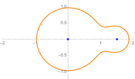
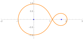
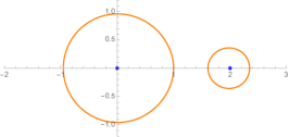
Figure 3. For $s=1$, $t=0.1$ and for the values (from left to right) $L=1.5$, $L=\lambda(0.1)\approx 1.7024$ and $L=2$, we display in the $x$-plane the locus $\Gamma$ in orange and the two finite poles of $\mathsf{x}^{{\rm A}+{\rm B}}$ (at $0$ and $L$) in blue.

$\bullet$ If $L<s\lambda(t)$, we have $\mathsf{Disc}<0$. Then we have two real ramification points satisfying

$$r_{-}(t)<0<L<r_{+}(t)$$

and a pair of complex conjugate ones. When $t\rightarrow 0$ they behave as

(88) $$r_{\pm}(t)=\pm s+\frac{sL(2s\mp L)}{2(s\mp L)^{2}}t+O(t^{2})\,,\qquad b_{\pm}(t)=\pm 2s+\frac{sL}{s\mp L}t+O(t^{2})\,.$$

$\Gamma$ is a topological circle and the two complex ramification points belong to the bounded connected component of $\Sigma^{{\rm A}+{\rm B}}\setminus\Gamma$. Letting $I=(r_{-}(t),r_{+}(t))$, we have a parametrisation $\gamma_{\pm}:I\rightarrow\Gamma\cap\mathbb{H}_{\pm}$ given by $\gamma_{\pm}(\xi)=\xi\pm{\rm i}\Upsilon_{+}(\xi)$. We call $J=(b_{-}(t),b_{+}(t))$.

$\bullet$ If $L=s\lambda(t)$, we have $\mathsf{Disc}=0$. Then we have three real ramification points satisfying

$$r_{-}(t)<0<r_{0}(t)<L<r_{+}(t)\,,$$

where $r_{0}(t)$ is double. When $t\rightarrow 0$, the two extreme ones behave as in (88) and the double one as

$$r_{0}(t)=s\Big{(}1+\frac{t^{1/3}}{2}+O(t^{2/3})\Big{)}\,,\qquad b_{0}(t)=2s\Big{(}1-\frac{3t^{2/3}}{8}+O(t)\Big{)}\,.$$

$\Gamma$ is a union of two topological circles meeting at $r_{0}(t)$. We can still parametrise $\Gamma\cap\mathbb{H}_{\pm}$ with $\gamma_{\pm}$ given above, except that the range is now $I=(r_{-}(t),r_{+}(t))\setminus\{r_{0}(t)\}$. We call $J=(b_{-}(t),b_{+}(t))\setminus\{b_{0}(t)\}$.

$\bullet$ If $L>s\lambda(t)$, we have $\mathsf{Disc}>0$. Then we have four real ramification points satisfying

$$r_{-}(t)<0<r_{+}(t)<\tilde{r}_{-}(t)<L<\tilde{r}_{+}(t).$$

When $t\rightarrow 0$, the two first ones behave as in (88), while the two last ones behave like

$$\tilde{r}_{\pm}(t)=L\pm\frac{sL}{\sqrt{L^{2}-s^{2}}}\sqrt{t}-\frac{s^{4}L}{(L^{2}-s^{2})^{2}}t+O(t^{3/2})\,,\qquad\quad\tilde{b}_{\pm}(t)=\Big{(}L+\frac{s^{2}}{L}\Big{)}\pm\frac{2s\sqrt{L^{2}-s^{2}}}{L}\sqrt{t}+O(t)\,.$$

$\Gamma$ is a disjoint union of two topological circles. Letting $I=(r_{-}(t),r_{+}(t))\cup(\tilde{r}_{-}(t),\tilde{r}_{+}(t))$, we have a parametrisation $\gamma_{\pm}:I\rightarrow\Gamma\cap\mathbb{H}_{\pm}$ with same formula as above. We call $J=(b_{-}(t),b_{+}(t))\cup(\tilde{b}_{-}(t),\tilde{b}_{+}(t))$.

Definition 6.4 (Parametrisations).

Recall the parametrisation of $\gamma_{\pm}:I\rightarrow\Gamma\cap\mathbb{H}_{\pm}$ is given by

$$\gamma_{\pm}(\xi)=\xi\pm{\rm i}\Upsilon_{+}(\xi)\,,$$

with $\Upsilon_{+}(\xi)$ defined in (87). We introduce the parametrisation $c\coloneqq\mathsf{x}^{{\rm A}+{\rm B}}\circ\gamma_{+}:I\rightarrow J$, which is equal to

(89) $$c(\xi)=2\xi-\frac{L}{2}+\frac{s^{2}-\sqrt{(L^{2}+s^{2})^{2}-4ts^{2}L^{2}-4(L^{2}+s^{2}-2ts^{2})L\xi+4L^{2}\xi^{2}}}{2(2\xi-L)}\,.$$

Although it is not manifest, this expression is regular at $\xi=L/2$. By design, for $\xi\in I$ the arguments inside each squareroot in $\gamma_{+}$ and $\Upsilon_{+}$ (87) are positive and we choose their nonnegative determination.

Lemma 6.5 (Properties of the parametrisations).

For any real ramification point $r$ and $t\in(0,1)$, $c^{\prime}(r)$ is finite and non-zero and there exists a constant $c_{r}>0$ such that

$$\Upsilon_{+}(\xi)\,\,\mathop{\sim}_{\begin{subarray}{c}\xi\in I\\ \xi\rightarrow r\end{subarray}}c_{r}|\xi-r|^{\frac{m}{2}}\,,$$

where $m=1$ if $r$ is simple and $m=2$ if $r$ is double. Besides, this asymptotic equivalence can be differentiated with respect to $\xi$.

Proof.

The first part is a computation. For the second part we remark that $\Upsilon_{+}(\xi)^{2}=-A(\xi)+\sqrt{B(\xi)}$, where $A,B$ are polynomials that can be read from (87) satisfying $A(\xi)\leq\sqrt{B(\xi)}$. We have $\Upsilon_{+}(r)=0$ but one can check that for $t\in(0,1)$ the roots of $A$ are not roots of $\tilde{Q}$. By comparing with (85) we find $B(\xi)-A^{2}(\xi)=-\tilde{Q}(\xi)$. Hence

$$\Upsilon_{+}(\xi)^{2}=\frac{B(\xi)-A(\xi)^{2}}{A(\xi)+\sqrt{B(\xi)}}$$

is analytic near $\xi=r$ with a zero of order $m$. ∎

Lemma 6.6 (Principal sheet).

Let $\mathcal{C}$ be the unbounded connected component of $\Sigma^{{\rm A}+{{\rm B}}}\setminus\Gamma$ (the component containing $\infty$ in the $x$ coordinate) and $\mathcal{C}_{\pm}=\mathcal{C}\cap\mathbb{H}_{\pm}$. Then $\mathsf{x}^{{\rm A}+{\rm B}}(\mathcal{C}_{\pm})\subseteq\mathbb{H}_{\pm}$ and $\mathsf{x}^{{\rm A}+{\rm B}}$ restricts to a biholomorphic map from $\mathcal{C}$ to $\widehat{\mathbb{C}}\setminus\overline{J}$.

Proof.

This is an elementary topological argument.

By construction, for $M>0$ large enough we have $\pm{\rm i}M\in\mathcal{C}_{\pm}$ while (86) implies that the sign of ${\rm Im}\,\mathsf{x}^{{\rm A}+{\rm B}}$ is $\pm 1$. The map ${\rm sgn}({\rm Im}\,\mathsf{x}^{{\rm A}+{\rm B}})$ is continuous on $\mathcal{C}_{\pm}$ and each of these two domains are connected, so we deduce that ${\rm sgn}({\rm Im}\,\mathsf{x}^{{\rm A}+{\rm B}})=\pm 1$ on $\mathcal{C}_{\pm}$, justifying the first claim.

Denote $\partial\mathcal{C}_{+}$ the boundary of $\mathcal{C}_{+}$ in the Riemann sphere $\Sigma^{{\rm A}+{\rm B}}$. Then, pick $x_{0}^{\pm}\in\mathbb{H}_{\pm}\setminus\overline{\mathcal{C}_{\pm}}$, introduce $i_{\pm}(x)=\frac{1}{x-x_{0}^{\pm}}$ that we consider as an automorphism of the Riemann sphere, and set $\mathcal{C}_{\pm}^{\prime}=i_{\pm}(\mathcal{C}_{\pm})$. The map $f_{\pm}=i_{\pm}\circ\mathsf{x}^{{\rm A}+{\rm B}}\circ i_{\pm}^{-1}$ is continuous on the bounded domain $\overline{\mathcal{C}_{\pm}^{\prime}}\subset\mathbb{C}$, holomorphic in $\mathcal{C}_{\pm}^{\prime}$ with image included in $i_{\pm}(\mathbb{H}_{\pm})$, and $\partial\mathcal{C}^{\prime}_{\pm}=i_{\pm}(\partial\mathcal{C}_{\pm})$ is a Jordan curve. After we justify that the restriction of $\mathsf{x}^{{\rm A}+{\rm B}}$ to $\partial\mathcal{C}_{\pm}^{\prime}$ is a homeomorphism onto $i_{\pm}(\mathbb{R}\cup\{\infty\})$, a classical theorem of complex analysis [SZ52, Chapter IV, §11] implies that $f_{\pm}$ gives a biholomorphic map from $\mathcal{C}^{\prime}_{\pm}$ onto $i_{\pm}(\mathbb{H}_{\pm})$. Hence, the restriction of $\mathsf{x}^{{\rm A}+{\rm B}}$ to $\mathcal{C}_{\pm}$ is biholomorphic onto $\mathbb{H}_{\pm}$. Together with $\mathsf{x}^{{\rm A}+{\rm B}}(\mathcal{C}_{\pm})\subset\mathbb{H}_{\pm}$ and the fact that $\mathsf{x}^{{\rm A}+{\rm B}}(\mathcal{C}\cap\mathbb{R})=\mathbb{R}\setminus\overline{J}$ (direct consequence of the variations of the restriction of $\mathsf{x}^{{\rm A}+{\rm B}}$ on $\mathbb{R}$), this implies that $\mathsf{x}^{{\rm A}+{\rm B}}$ is a biholomorphic map from $\mathcal{C}$ to $\widehat{\mathbb{C}}\setminus\overline{J}$.

To justify the injectivity on the boundary, we remark that the map $x\mapsto{\rm Re}\,x$ restricts to a homeomorphism $\psi_{\pm}$ from $\partial\mathcal{C}_{\pm}\setminus\{\infty\}$ to $\mathbb{R}$, which is real-analytic away from the ramification points. Then $h_{\pm}=\mathsf{x}^{{\rm A}+{\rm B}}\circ\psi^{-1}_{\pm}:\mathbb{R}\rightarrow\mathbb{R}$ is continuous, and away from the ramification points it is real-analytic. As $\Gamma$ does not contain ramification points (cf. Footnote 10) and the differential of $\mathsf{x}^{{\rm A}+{\rm B}}$ is $\mathbb{C}$-linear, $h_{\pm}^{\prime}$ does not vanish away from ramification points. Hence, $h_{\pm}$ is strictly monotone and $\mathsf{x}^{{\rm A}+{\rm B}}$ is injective on $\partial\mathcal{C}_{\pm}\setminus\{\infty\}$. Since the latter does not contain the poles of $\mathsf{x}^{{\rm A}+{\rm B}}$ located at $0,L,\infty$, we conclude that $\mathsf{x}^{{\rm A}+{\rm B}}$ is injective on $\partial\mathcal{C}_{\pm}$, as desired. ∎

6.5   Distributional form

It is well-known that the $(0,1)$-moments come from a positive measure on $\mathbb{R}$ (called equilibrium measure). The BBP phase transition manifests itself when $t\rightarrow 0$ by a change of the topology of the support: if $L<s$ the support is a segment close to $[-2s,2s]$, while if $L>s$ it also contains a second segment of width $O(\sqrt{t})$ around $L+\frac{s^{2}}{L}$. Section 6.4 revisited this transition and contains all the necessary information to describe explicitly the equilibrium measure for $t\in(0,1)$.

Lemma 6.7 (Law of large numbers).

For any polynomial $f$, we have

$$\mathbb{E}\big{[}{\rm Tr}f(A_{N}+B_{N})]\mathop{=}_{N\rightarrow\infty}N\int_{J}f\mathrm{d}\mu_{0,1}+O\Big{(}\frac{1}{N}\Big{)}\,,$$

where $\mu_{0,1}$ is the probability measure with support $\overline{J}$, whose pullback by the parametrisation $c:I\rightarrow J$ is

$$c^{*}\mu_{0,1}=\frac{\Upsilon_{+}(\xi)}{\pi s^{2}}\mathbf{1}_{I}(\xi)\mathrm{d}\xi\,.$$

If $L\leq s\lambda(t)$, the support consists of one segment. If $L>s\lambda(t)$, the support consists of two segments, and $\mu_{0,1}$ assigns mass $t$ to the rightmost one.

Remark 6.8.

From (87)-(89) we can determine the behavior of the equilibrium measure when $t\rightarrow 0$. As expected, it becomes semi-circular at the macroscopic level:

$$\lim_{t\rightarrow 0}\frac{\mathrm{d}\mu_{{\rm eq}}(\mathsf{x})}{\mathrm{d}\mathsf{x}}=\frac{\sqrt{4s^{2}-\mathsf{x}^{2}}}{2\pi s^{2}}\,\mathbf{1}_{[-2s,2s]}(\mathsf{x})$$

uniformly for $\mathsf{x}\in\mathbb{R}$. Besides, if $L>s\lambda(0)=s$, the measure also has in its support a segment with size of order $\sqrt{t}$ and mass $t$, where it also looks semi-circular:

$$\frac{\mathrm{d}\mu_{0,1}(\mathsf{x}(\mathsf{v}))}{\mathrm{d}\mathsf{v}}\mathop{=}_{t\rightarrow 0}\frac{2t\sqrt{1-\mathsf{v}^{2}}}{\pi}\mathbf{1}_{[-1,1]}(\mathsf{v})+O(t^{3/2}),\qquad\text{ where}\,\,\mathsf{x}(\mathsf{v})=L+\frac{s^{2}}{L}+\frac{2s}{L}\sqrt{L^{2}-s^{2}}\sqrt{t}\,\mathsf{v}$$

uniformly for real $\mathsf{v}$ on any compact set.

Proof.

From (76) we get for $N\rightarrow\infty$

$$\mathbb{E}\big{[}{\rm Tr}f(A_{N}+B_{N})\big{]}\mathop{=}_{N\rightarrow\infty}\,\,N\,\mathcal{M}_{0,1}[f]+O\Big{(}\frac{1}{N}\Big{)},\;\text{ with}\,\,\mathcal{M}_{0,1}[f]\coloneqq-\mathop{{\rm Res}}_{x=\infty}f\big{(}\mathsf{x}^{{\rm A}+{\rm B}}(x)\big{)}\mathsf{w}(x)\mathrm{d}\mathsf{x}^{{\rm A}+{\rm B}}(x)\,.$$

We use the formula (75) for $\big{(}\mathsf{x}^{{\rm A}+{\rm B}}(x),\mathsf{w}(x)\big{)}$ and move the contour in $\Sigma^{{\rm A}+{\rm B}}$ to rewrite

(90) $$\begin{split}\mathcal{M}_{0,1}[f]&=\frac{1}{s^{2}}\mathop{{\rm Res}}_{x=\infty}f\big{(}\mathsf{x}^{{\rm A}+{\rm B}}(x)\big{)}\big{(}x-\mathsf{x}^{{\rm A}+{\rm B}}(x)\big{)}\mathrm{d}\mathsf{x}^{{\rm A}+{\rm B}}(x)=\frac{1}{s^{2}}\mathop{{\rm Res}}_{x=\infty}f\big{(}\mathsf{x}^{{\rm A}+{\rm B}}(x)\big{)}\,x\mathrm{d}\mathsf{x}^{{\rm A}+{\rm B}}(x)\\ &=\frac{-1}{2{\rm i}\pi s^{2}}\oint_{\Gamma}f\big{(}\mathsf{x}^{{\rm A}+{\rm B}}(x)\big{)}\,x\,\mathrm{d}\mathsf{x}^{{\rm A}+{\rm B}}(x)\,,\end{split}$$

where $\Gamma$ is equipped with the counterclockwise orientation. Recall that $x\in\Gamma$ is parametrised by $\xi\in I\subset\mathbb{R}$ as $x=\gamma_{\pm}(\xi)=\xi\pm{\rm i}\Upsilon_{+}(\xi)$, and that $c(\xi)=\mathsf{x}^{{\rm A}+{\rm B}}(\xi\pm{\rm i}\Upsilon_{+}(\xi))$ given in (89) does not depend on the sign $\pm$. In consequence, (90) can be converted to an integral over $I$ (oriented from left to right)

$$\mathcal{M}_{0,1}[f]=\frac{-1}{2{\rm i}\pi s^{2}}\int_{I}f(c(\xi))\Big{(}\big{(}\xi-{\rm i}\Upsilon_{+}(\xi)\big{)}-\big{(}\xi+{\rm i}\Upsilon_{+}(\xi)\big{)}\Big{)}\mathrm{d}c(\xi)=\int_{I}f(c(\xi))\,\frac{\Upsilon_{+}(\xi)\mathrm{d}c(\xi)}{\pi s^{2}}\,,$$

and we recognise the announced result.

The support of this measure is $c(\overline{I})=\overline{J}$. It was described in Section 6.4 and we saw that it depends on the relative position of $L$ and $s\lambda(t)$. When $L>s\lambda(t)$, it consists of two segments, and the rightmost one (call it $J_{2}$) is the $\mathsf{x}^{{\rm A}+{\rm B}}$-image of the component of $\Gamma$ surrounding $x=L$ (call it $\Gamma_{2}$). We can repeat the previous manipulations to compute the mass of $J_{2}$ as the contour integral in the $x$-plane

$$\mu_{{\rm eq}}[J_{2}]=\frac{1}{2{\rm i}\pi}\oint_{\Gamma_{2}}\mathsf{w}(x)\,\mathrm{d}\mathsf{x}^{{\rm A}+{\rm B}}(x)\,.$$

In view of (75), the integrand is meromorphic inside $\Gamma_{2}$ with a pole at $x=L$, so the integral is evaluated by a residue at this point, and we find $\mu_{{\rm eq}}[J_{2}]=t$. ∎

We go further by demonstrating that $(0,2)$ moments come from a measure, while the $(g,n)$ moments for $2g-2+n>0$ come from a finite order distribution. The support of these measures or distributions is independent of $(g,n)$ and corresponds to $\overline{J}$ introduced in Section 6.4.

Proposition 6.9 (Subleading correction to the law of large numbers).

We have when $N\rightarrow\infty$

$$\mathbb{E}\big{[}{\rm Tr}\,f(A_{N}+B_{N})\big{]}=N\int_{J}f\,\mathrm{d}\mu_{0,1}+\frac{1}{N}\int_{J}f^{\prime\prime\prime}\,\mathrm{d}\mu_{1,1}+O\Big{(}\frac{1}{N^{3}}\Big{)}\,,$$

where $\mu_{1,1}$ is the signed measure of mass $0$ on $\overline{J}$ given by

$$c^{*}\mu_{1,1}=-\frac{s^{2}}{24\pi}\,\frac{c^{\prime}(\xi)\Upsilon_{+}^{\prime}(\xi)}{1+(\Upsilon_{+}^{\prime}(\xi))^{2}}\ \mathbf{1}_{I}(\xi)\mathrm{d}\xi\,.$$

If $L>s\lambda(0)=s$, then $\mu_{1,1}$ gives mass $\frac{s^{6}t(1-t)}{6L^{3}}$ to the rightmost segment. Besides, when $t\rightarrow 0$

$$\lim_{t\rightarrow 0}\frac{\mathrm{d}\mu_{1,1}(\mathsf{x})}{\mathrm{d}\mathsf{x}}=\frac{\mathsf{x}\sqrt{4s^{2}-\mathsf{x}^{2}}}{48\pi}\mathbf{1}_{[-2s,2s]}(\mathsf{x})$$

uniformly for $\mathsf{x}\in\mathbb{R}$. Besides, if $L>s\lambda(t)$, setting $\mathsf{x}(\mathsf{v})=L+\frac{s^{2}}{L}+\frac{2s}{L}\sqrt{L^{2}-s^{2}}\sqrt{t}\,\mathsf{v}$,

$$\frac{\mathrm{d}\mu_{1,1}(\mathsf{x}(\mathsf{v}))}{\mathrm{d}\mathsf{v}}\mathop{=}_{t\rightarrow 0}\frac{s^{3}\sqrt{L^{2}-s^{2}}}{12\pi L}\,\mathsf{v}\sqrt{1-\mathsf{v}^{2}}\,\sqrt{t}+O(t)$$

uniformly for $\mathsf{v}$ in any compact of $\mathbb{R}$.

Proposition 6.10 (Central limit theorem).

Let $f$ be a polynomial. The random variable

$$\varkappa_{N}[f]\coloneqq{\rm Tr}\,f(A_{N}+B_{N})-N\int_{J}f\mathrm{d}\mu_{0,1}$$

converges in law to a centered Gaussian random variable as $N\to\infty$, with variance

$$\frac{1}{2\pi^{2}}\int_{I^{2}}\ln\Bigg{|}\frac{\gamma_{+}(\xi_{1})-\overline{\gamma_{+}(\xi_{2})}}{\gamma_{+}(\xi_{1})-\gamma_{+}(\xi_{2})}\Bigg{|}\,f^{\prime}(c(\xi_{1}))f^{\prime}(c(\xi_{2}))\mathrm{d}c(\xi_{1})\mathrm{d}c(\xi_{2})\,.$$

In other words, for any polynomial $f$, the random variable $\varkappa_{N}[f]$ converges in law to $\frac{1}{\sqrt{\pi}}\langle\mathscr{G},f^{\prime}\circ\mathsf{x}^{{\rm A}+{\rm B}}\rangle$, where $\mathscr{G}$ is the restriction to $\Gamma\cap\mathbb{H}_{+}$ of the Gaussian free field in $\mathbb{H}_{+}$ with Dirichlet boundary condition.

Proposition 6.11 (Leading asymptotics of third order cumulants).

If $L\neq s\lambda(t)$, we have when $N\rightarrow\infty$

(91) $$\mathbb{E}^{\circ}\big{[}{\rm Tr}\,f(A_{N}+B_{N}),{\rm Tr}\,f(A_{N}+B_{N}),{\rm Tr}\,f(A_{N}+B_{N})\big{]}=\frac{1}{N}\int_{J^{3}}f^{\prime}\otimes f^{\prime}\otimes f^{\prime}\,\mathrm{d}\mu_{0,3}+O\Big{(}\frac{1}{N^{3}}\Big{)}\,,$$

where $\mu_{0,3}$ is a finite signed measure supported on $\overline{J}^{3}$ such that

(92) $$(c,c,c)^{*}\mu_{0,3}=\frac{{\rm i}s^{2}}{8\pi^{3}}\sum_{\begin{subarray}{c}\epsilon_{1},\epsilon_{2},\epsilon_{3}=\pm 1\\ i=1,2,3\end{subarray}}\frac{\epsilon_{1}\epsilon_{2}\epsilon_{3}\gamma_{\epsilon_{i}}^{\prime}(\xi_{i})\,\mathbf{1}_{I^{3}}(\xi_{1},\xi_{2},\xi_{3})\mathrm{d}\xi_{1}\mathrm{d}\xi_{2}\mathrm{d}\xi_{3}}{c^{\prime}(\xi_{i})\big{(}\gamma_{\epsilon_{i}}(\xi_{i})-\gamma_{\epsilon_{j}}(\xi_{j})\big{)}\big{(}\gamma_{\epsilon_{i}}(\xi_{i})-\gamma_{\epsilon_{k}}(\xi_{k})\big{)}}$$

(the explicit expression is long and not particularly enlightening). If $J^{(1)},J^{(2)},J^{(3)}$ is any triple of connected components of $\overline{J}$, we have $\mu_{0,3}[J^{(1)}\times J^{(2)}\times J^{(3)}]=0$.

If $L=s\lambda(t)$, (92) develops a double pole at $\xi_{i}=r_{0}(t)$ and one should rather consider $\mu_{0,3}$ as a distribution: (91) still holds but one should add to $\Upsilon_{+}(\xi_{j})$ a term $\eta\cdot\theta(\frac{\xi_{j}-r_{0}(t)}{\eta})$ where $\eta>0$ is small enough and $\theta$ is a smooth function with support $[-1,1]$ and $\theta(0)=1$ (the result does not depend on such $\eta$ and $\theta$).

Proof of Proposition 6.9.

We first observe that if $h$ is a meromorphic function on $\Sigma^{{\rm A}+{\rm B}}$ without pole at $\infty$ and $f$ is a polynomial, we have by integration by parts

$$\mathop{{\rm Res}}_{x=\infty}f\big{(}\mathsf{x}^{{\rm A}+{\rm B}}(x)\big{)}\mathrm{d}h(x)=-\mathop{{\rm Res}}_{x=\infty}f^{\prime}\big{(}\mathsf{x}^{{\rm A}+{\rm B}}(x)\big{)}h(x)\mathrm{d}\mathsf{x}^{{\rm A}+{\rm B}}(x)\,.$$

Recalling Definition 6.2 for the operator $\nabla$, we have likewise for $n\in\mathbb{Z}_{>0}$

(93) $$\mathop{{\rm Res}}_{x=\infty}f\big{(}\mathsf{x}^{{\rm A}+{\rm B}}(x)\big{)}\mathrm{d}\big{(}\nabla^{n}h(x)\big{)}=(-1)^{n+1}\mathop{{\rm Res}}_{x=\infty}f^{(n+1)}\big{(}\mathsf{x}^{{\rm A}+{\rm B}}(x)\big{)}h(x)\mathrm{d}\mathsf{x}^{{\rm A}+{\rm B}}(x)\,.$$

The order $1/N$ term in the $N\rightarrow\infty$ asymptotic expansion of $\mathbb{E}\big{[}{\rm Tr}\,f(A_{N}+B_{N})\big{]}$ is

$$\mathcal{M}_{1,1}[f]=-\mathop{{\rm Res}}_{x=\infty}f\big{(}\mathsf{x}^{{\rm A}+{\rm B}}(x)\big{)}\,\omega_{1,1}^{{\rm A}+{\rm B}}(x)\,.$$

As $\omega_{1,1}$ has poles at the ramification points, we cannot directly move the contour to $\Gamma$ to rewrite it as an integral over $J$. Instead, we first use integration by parts. With the formula (80) for $\omega_{1,1}$, using the identity (93), we get

(94) $$\mathcal{M}_{1,1}[f]=\frac{s^{2}}{24}\mathop{{\rm Res}}_{x=\infty}f^{\prime\prime\prime}\big{(}\mathsf{x}^{{\rm A}+{\rm B}}(x)\big{)}\frac{(\mathrm{d}\mathsf{x}^{{\rm A}+{\rm B}})^{2}}{\mathrm{d}x}\,.$$

Now, recalling the expression (84) for $\mathsf{x}^{{\rm A}+{\rm B}}$, the integrand has poles only at $x=0,L,\infty$, so we can move the contour from $\infty$ to $\Gamma$, and proceed as in the proof of Lemma 6.7 to obtain

(95) $$\begin{split}\mathcal{M}_{1,1}[f]&=\frac{s^{2}}{48{\rm i}\pi}\,\int_{I}f^{\prime\prime\prime}(c(\xi))\frac{(\mathrm{d}c(\xi))^{2}}{\mathrm{d}\xi}\Big{(}\frac{1}{1+{\rm i}\Upsilon_{+}^{\prime}(\xi)}-\frac{1}{1-{\rm i}\Upsilon_{+}^{\prime}(\xi)}\Big{)}\\ &=-\frac{s^{2}}{24\pi}\int_{I}f^{\prime\prime\prime}(c(\xi))\,\frac{c^{\prime}(\xi)\Upsilon^{\prime}(\xi)\mathrm{d}\xi}{1+(\Upsilon_{+}^{\prime}(\xi))^{2}}\,\mathrm{d}c(\xi)\,.\end{split}$$

Replacing $f^{\prime\prime\prime}$ with $1$ in (94) computes $\mu_{1,1}[J]$, and it is equal to $0$ because the integrand has vanishing residue at $\infty$. If $L>s$, we can distinguish the mass of the rightmost segment

$$\mu_{1,1}[J_{2}]=\frac{s^{4}}{24}\mathop{{\rm Res}}_{x=L}\Big{(}\frac{t}{(x-L)^{2}}+\frac{1-t}{x^{2}}\Big{)}\mathrm{d}\mathsf{x}^{{\rm A}+{\rm B}}(x)=\frac{s^{6}t(1-t)}{6L^{3}}\,.$$

∎

Proof of Proposition 6.10.

In (76) we read that the variance of $\varkappa_{N}[f]$ when $N\rightarrow\infty$ is

$${\rm Var}[\varkappa_{N}[f]\big{]}=\mathcal{M}_{0,2}[f]+o(1)\,,$$

where

(96) $$\mathcal{M}_{0,2}[f]\coloneqq\mathop{{\rm Res}}_{x_{1}=\infty}\mathop{{\rm Res}}_{x_{2}=\infty}\omega_{0,2}^{{\rm A}+{\rm B}}(x_{1},x_{2})\prod_{j=1}^{2}f\big{(}\mathsf{x}^{{\rm A}+{\rm B}}(x_{j})\big{)}\mathrm{d}\mathsf{x}^{{\rm A}+{\rm B}}(x_{j})\,.$$

Furthermore, from (76) we know that $\varkappa_{N}[f]$ has mean $O(N^{-1})=o(1)$, and for $n\geq 3$, that its $n$-th cumulant is $O(N^{2-n})=o(1)$. This implies that the moments of $\varkappa_{N}[f]$ converge to the moments of a centered Gaussian random variable with variance $\mathcal{M}_{0,2}[f]$. By the method of moments, this implies convergence in law of $\varkappa_{N}[f]$ towards this Gaussian.

Recall from Proposition 6.3 the formula

(97) $$\omega_{0,2}^{{\rm A}+{\rm B}}(x_{1},x_{2})=\frac{\mathrm{d}x_{1}\mathrm{d}x_{2}}{(x_{1}-x_{2})^{2}}-\frac{\mathrm{d}\mathsf{x}^{{\rm A}+{\rm B}}(x_{1})\mathrm{d}\mathsf{x}^{{\rm A}+{\rm B}}(x_{2})}{\big{(}\mathsf{x}^{{\rm A}+{\rm B}}(x_{1})-\mathsf{x}^{{\rm A}+{\rm B}}(x_{2})\big{)}^{2}}\,.$$

The residues in (96) can be realised by integration along $x_{j}$ on clockwise-oriented circles with large radii $\rho_{1}$ and $\rho_{2}$, and we can choose $\rho_{2}>\rho_{1}$. Calling $C_{1},C_{2}$ those circles with counterclockwise orientation, we get

$$\mathcal{M}_{0,2}[f]=\frac{-1}{4\pi^{2}}\oint_{C_{1}}\oint_{C_{2}}\bigg{(}\frac{\mathrm{d}x_{1}\mathrm{d}x_{2}}{(x_{1}-x_{2})^{2}}-\frac{\mathrm{d}\mathsf{x}^{{\rm A}+{\rm B}}(x_{1})\mathrm{d}\mathsf{x}^{{\rm A}+{\rm B}}(x_{2})}{\big{(}\mathsf{x}^{{\rm A}+{\rm B}}(x_{1})-\mathsf{x}^{{\rm A}+{\rm B}}(x_{2})\big{)}^{2}}\bigg{)}\prod_{j=1}^{2}f\big{(}\mathsf{x}^{{\rm A}+{\rm B}}(x_{j})\big{)}\,.$$

As each term in the integrand is regular on $C_{1}\times C_{2}$, we can split the integral into a sum of two. For the second term, we can change variable to $\mathsf{x}_{j}=\mathsf{x}^{{\rm A}+{\rm B}}(x_{j})$. With respect to $\mathsf{x}_{1}$ the integrand is holomorphic in the bounded connected component of $\mathbb{C}\setminus\mathsf{x}^{{\rm A}+{\rm B}}(C_{1})$, therefore the integral vanishes. For the first term, we can move $C_{1}$ to $\Gamma$, and then move $C_{2}$ to a contour $\Gamma^{+\eta}$ slightly larger than $\Gamma$, at distance $\eta$ from the latter.

For simplicity of the computations, we assume $L<s\lambda(t)$ so that $C_{1}$ and $C_{2}$ have only one component (the argument transposes easily to the case $L\geq s\lambda(t)$). We use the notation $C_{j}^{\pm}\coloneqq C_{j}\cap\mathbb{H}_{\pm}$ for the oriented arcs ($-C_{j}^{\pm}$ is the arc $C_{j}^{\pm}$ with the opposite orientation); the endpoints of $C_{1}^{\pm}$ are $r_{\pm}(t)$ (see Section 6.4) and the endpoints of $C_{2}^{\pm}$ are $r_{\pm}(t)\pm\eta$.

The strategy is to perform integration by parts with respect to $x_{2}$ and $x_{1}$. This makes appear a logarithm. In order to avoid discontinuities in the definition of complex logarithms, we will try to use real logarithms. For this purpose we decompose the integral into four pieces:

$$\begin{split}\mathcal{M}_{0,2}[f]=&\frac{-1}{4\pi^{2}}\Bigg{(}\int_{C_{1}^{+}}\int_{C_{2}^{+}}+\int_{C_{1}^{-}}\int_{C_{2}^{-}}+\int_{C_{1}^{+}}\int_{C_{2}^{-}}+\int_{C_{1}^{-}}\int_{C_{2}^{+}}\Bigg{)}\frac{\mathrm{d}x_{1}\mathrm{d}x_{2}}{(x_{1}-x_{2})^{2}}\prod\limits_{j=1}^{2}f\big{(}\mathsf{x^{{\rm A}+{\rm B}}}(x_{j})\big{)}\\ =&\frac{-1}{4\pi^{2}}\int_{-C_{1}^{+}}\int_{-C_{2}^{+}}\Bigg{(}\frac{\mathrm{d}x_{1}\mathrm{d}x_{2}}{(x_{1}-x_{2})^{2}}\prod\limits_{j=1}^{2}f\big{(}\mathsf{x^{{\rm A}+{\rm B}}}(x_{j})\big{)}+\frac{\mathrm{d}\overline{x}_{1}\mathrm{d}\overline{x}_{2}}{(\overline{x}_{1}-\overline{x}_{2})^{2}}\prod\limits_{j=1}^{2}f\big{(}\mathsf{x^{{\rm A}+{\rm B}}}(\overline{x}_{j})\big{)}\\ &-\frac{\mathrm{d}x_{1}\mathrm{d}\overline{x}_{2}}{(x_{1}-\overline{x}_{2})^{2}}f\big{(}\mathsf{x^{{\rm A}+{\rm B}}}(x_{1})\big{)}f\big{(}\mathsf{x^{{\rm A}+{\rm B}}}(\overline{x}_{2})\big{)}-\frac{\mathrm{d}\overline{x}_{1}\mathrm{d}x_{2}}{(\overline{x}_{1}-x_{2})^{2}}f\big{(}\mathsf{x^{{\rm A}+{\rm B}}}(\overline{x}_{1})\big{)}f\big{(}\mathsf{x^{{\rm A}+{\rm B}}}(x_{2})\big{)}\Bigg{)}\end{split}$$

where we have used that $\int_{C_{j}^{-}}h(x_{j})\mathrm{d}x_{j}=\int_{-C_{j}^{+}}h(\overline{x}_{j})\mathrm{d}\overline{x}_{j}$ to get the second equality. We claim that we can replace $f\big{(}\mathsf{x}^{{\rm A}+{\rm B}}(\overline{x}_{j})\big{)}$ with $f\big{(}\mathsf{x}^{{\rm A}+{\rm B}}(x_{j})\big{)}$ in these integrals. For $x_{1}\in C_{1}^{+}$ this is clear: we have $\mathsf{x}^{{\rm A}+{\rm B}}(\overline{x}_{1})=\mathsf{x}^{{\rm A}+{\rm B}}(x_{1})$ hence $f\big{(}\mathsf{x}^{{\rm A}+{\rm B}}(\overline{x}_{1})\big{)}=f\big{(}\mathsf{x}^{{\rm A}+{\rm B}}(x_{1})\big{)}$. For $x_{2}\in C_{2}^{+}=\Gamma^{+\eta}$, we only have

$$\underset{\eta\to 0}{\lim}\,\big{(}f(\mathsf{x}^{{\rm A}+{\rm B}}(\overline{x}_{2}))-f(\mathsf{x}^{{\rm A}+{\rm B}}(x_{2}))\big{)}=0\,.$$

and we have to justify that

(98) $$\underset{\eta\to 0}{\lim}\int_{-C_{1}^{+}}\int_{-C_{2}^{+}}\frac{\mathrm{d}\overline{x}_{1}\mathrm{d}\overline{x}_{2}}{(\overline{x}_{1}-\overline{x}_{2})^{2}}f\big{(}\mathsf{x}^{{\rm A}+{\rm B}}(x_{1})\big{)}\Big{[}f\big{(}\mathsf{x}^{{\rm A}+{\rm B}}(\overline{x}_{2})\big{)}-f\big{(}\mathsf{x}^{{\rm A}+{\rm B}}(x_{2})\big{)}\Big{]}=0\,.$$

We start with the integral in the left-hand side for fixed $\eta>0$, and first perform integration by parts with respect to $x_{2}$. This does not create boundary terms because the endpoints of $\Gamma^{+\eta}\cap\mathbb{H}_{\pm}$ are on the real line and the last factor in (98) vanishes there. We then perform integration by parts with respect to $x_{1}$. It creates a boundary term and makes appear a complex logarithm. For $(x_{1},x_{2})\in C_{1}^{+}\times C_{2}^{+}$ we have $(\overline{x}_{1}-\overline{x}_{2})\notin-{\rm i}\mathbb{R}$, so we can choose the complex logarithm having a cut on $-{\rm i}\mathbb{R}_{\geq 0}$ and coinciding with the real logarithm on $\mathbb{R}_{>0}$. This rewrites the left-hand side of (98) before taking the limit as

$$\begin{split}&\int_{-C_{1}^{+}}\int_{-C_{2}^{+}}\ln(\overline{x}_{1}-\overline{x}_{2})f^{\prime}\big{(}\mathsf{x}^{{\rm A}+{\rm B}}(x_{1})\big{)}\Big{[}f^{\prime}\big{(}\mathsf{x}^{{\rm A}+{\rm B}}(\overline{x}_{2})\big{)}\mathrm{d}\mathsf{x}^{{\rm A}+{\rm B}}(\overline{x}_{2})-f^{\prime}\big{(}\mathsf{x}^{{\rm A}+{\rm B}}(x_{2})\big{)}\mathrm{d}\mathsf{x}^{{\rm A}+{\rm B}}(x_{2})\Big{]}\mathrm{d}\mathsf{x}^{{\rm A}+{\rm B}}(x_{1})\\ &-\sum_{\epsilon=\pm 1}\int_{-C_{2}^{+}}\ln(b_{\epsilon}(t)-\overline{x}_{2})f(b_{\epsilon}(t))\Big{[}f^{\prime}\big{(}\mathsf{x}^{{\rm A}+{\rm B}}(\overline{x}_{2})\big{)}\mathrm{d}\mathsf{x}^{{\rm A}+{\rm B}}(\overline{x}_{2})-f^{\prime}\big{(}\mathsf{x}^{{\rm A}+{\rm B}}(x_{2})\big{)}\mathrm{d}\mathsf{x}^{{\rm A}+{\rm B}}(x_{2})\Big{]}\,.\end{split}$$

We can now apply dominated convergence by putting absolute values around the integrands and we get that the limit as $\eta\to 0$ is zero.

Therefore, we are led to carry out the following integrals:

(99) $$\begin{split}\mathcal{M}_{0,2}[f]&=\underset{\eta\to 0}{\lim}\,\Bigg{[}\frac{-1}{4\pi^{2}}\int_{-C_{1}^{+}}\int_{-C_{2}^{+}}\Bigg{(}\frac{\mathrm{d}x_{1}\mathrm{d}x_{2}}{(x_{1}-x_{2})^{2}}+\frac{\mathrm{d}\overline{x}_{1}\mathrm{d}\overline{x}_{2}}{(\overline{x}_{1}-\overline{x}_{2})^{2}}\Bigg{)}\prod\limits_{j=1}^{2}f\big{(}\mathsf{x^{{\rm A}+{\rm B}}}(x_{j})\big{)}\\ &\quad+\frac{1}{4\pi^{2}}\int_{-C_{1}^{+}}\int_{-C_{2}^{+}}\Bigg{(}\frac{\mathrm{d}x_{1}\mathrm{d}\overline{x}_{2}}{(x_{1}-\overline{x}_{2})^{2}}+\frac{\mathrm{d}\overline{x}_{1}\mathrm{d}x_{2}}{(\overline{x}_{1}-x_{2})^{2}}\Bigg{)}\prod\limits_{j=1}^{2}f\big{(}\mathsf{x^{{\rm A}+{\rm B}}}(x_{j})\big{)}\Bigg{]}\,.\end{split}$$

Again, we perform integration by parts with respect to $x_{2}$ and $x_{1}$. It turns out that the boundary terms in the two lines of (99) cancel each other. In the end, we obtain:

$$\begin{split}\mathcal{M}_{0,2}[f]=&\underset{\eta\to 0}{\lim}\,\Bigg{[}\frac{-1}{4\pi^{2}}\int_{-C_{1}^{+}}\int_{-C_{2}^{+}}\ln|x_{1}-x_{2}|^{2}\prod\limits_{j=1}^{2}f^{\prime}\big{(}\mathsf{x^{{\rm A}+{\rm B}}}(x_{j})\big{)}\mathrm{d}\mathsf{x^{{\rm A}+{\rm B}}}(x_{j})\\ &+\frac{1}{4\pi^{2}}\int_{-C_{1}^{+}}\int_{-C_{2}^{+}}\ln|x_{1}-\overline{x}_{2}|^{2}\prod\limits_{j=1}^{2}f^{\prime}\big{(}\mathsf{x^{{\rm A}+{\rm B}}}(x_{j})\big{)}\mathrm{d}\mathsf{x^{{\rm A}+{\rm B}}}(x_{j})\Bigg{]}\\ =&\frac{1}{4\pi^{2}}\int_{-C_{1}^{+}}\int_{-C_{1}^{+}}\ln\left|\frac{x_{1}-\overline{x}_{2}}{x_{1}-x_{2}}\right|^{2}\prod\limits_{j=1}^{2}f^{\prime}\big{(}\mathsf{x^{{\rm A}+{\rm B}}}(x_{j})\big{)}\mathrm{d}\mathsf{x^{{\rm A}+{\rm B}}}(x_{j}).\end{split}$$

Notice that thanks to the way the integral was split, only the real log is involved here and every term is integrable. Using the change of variable $x_{j}=\gamma_{+}(\xi_{j})$, we get the desired expression. ∎

Proof of Proposition 6.11.

The term we want to compute is

(100) $$\begin{split}\mathcal{M}_{0,3}[f]&\coloneqq-\mathop{{\rm Res}}_{x_{1}=\infty}\mathop{{\rm Res}}_{x_{2}=\infty}\mathop{{\rm Res}}_{x_{3}=\infty}\omega_{0,3}^{{\rm A}+{\rm B}}(x_{1},x_{2},x_{3})\prod_{i=1}^{3}f\big{(}\mathsf{x}^{{\rm A}+{\rm B}}(x_{i})\big{)}\\ &=\mathop{{\rm Res}}_{x_{1}=\infty}\mathop{{\rm Res}}_{x_{2}=\infty}\mathop{{\rm Res}}_{x_{3}=\infty}M_{0,3}(x_{1},x_{2},x_{3})\prod_{a=1}^{3}f^{\prime}\big{(}\mathsf{x}^{{\rm A}+{\rm B}}(x_{a})\big{)}\mathrm{d}\mathsf{x}^{{\rm A}+{\rm B}}(x_{a})\big{)}\,,\end{split}$$

where we have introduced

$$M_{0,3}(x_{1},x_{2},x_{3})=s^{2}\bigg{(}\sum_{i=1}^{3}\frac{\mathrm{d}x_{i}}{\mathrm{d}\mathsf{x}^{{\rm A}+{\rm B}}(x_{i})\,(x_{i}-x_{j})(x_{i}-x_{k})}\bigg{)}\,.$$

As in the previous proofs, we would like to move the three integration contours to $\Gamma$ and rewrite it as an integral over $I^{3}$, but this can be done only when the function

$$\Delta M_{0,3}(\xi_{1},\xi_{2},\xi_{3})\coloneqq\frac{1}{(2{\rm i}\pi)^{3}}\sum_{\epsilon_{1},\epsilon_{2},\epsilon_{3}=\pm 1}\epsilon_{1}\epsilon_{2}\epsilon_{3}\,M_{0,3}\big{(}\xi_{1}+{\rm i}\epsilon_{1}\Upsilon_{+}(\xi_{1}),\xi_{2}+{\rm i}\epsilon_{2}\Upsilon_{+}(\xi_{2}),\xi_{3}+{\rm i}\epsilon_{3}\Upsilon_{+}(\xi_{3})\big{)}$$

is integrable on $I^{3}$. The function $M_{0,3}$ has an alternative expression found in (79): it is of the form $\frac{F(x_{1},x_{2},x_{3})}{\tilde{Q}(x_{1})\tilde{Q}(x_{2})\tilde{Q}(x_{3})}$, where $F$ is a polynomial. We only need to check the local integrability of $\Delta M_{0,3}$ when $\xi_{i}$ approaches an endpoint of $I$, since these correspond to ramification points, i.e. roots of $\tilde{Q}$.

Assume $L\neq s\lambda(t)$. In this case we learned in Section 6.4 that all ramification points are simple. Let us take a triple $\mathbf{r}=(r^{(1)},r^{(2)},r^{(3)})$ of ramification points (possibly equal). With a partial fraction expansion we can find two triples of constants $\boldsymbol{\alpha}$, $\boldsymbol{\beta}$ such that

$$M_{0,3}(x_{1},x_{2},x_{3})=\prod_{j=1}^{3}\Big{(}\alpha^{(j)}+\frac{\beta^{(j)}}{x_{j}-r^{(j)}}\Big{)}+\tilde{M}_{0,3}(x_{1},x_{2},x_{3})\,.$$

Then $\Delta M_{0,3}(\xi_{1},\xi_{2},\xi_{3})=\prod_{j=1}^{3}\beta^{(j)}K_{r^{(j)}}(\xi_{j})+\Delta\tilde{M}_{0,3}(\xi_{1},\xi_{2},\xi_{3})$, where

$$K_{r}(\xi)=\frac{1}{2{\rm i}\pi}\bigg{(}\frac{1}{\xi+{\rm i}\Upsilon_{+}(\xi)-r}-\frac{1}{\xi-{\rm i}\Upsilon_{+}(\xi)-r}\bigg{)}=\frac{-1}{\pi}\,\frac{\Upsilon_{+}(\xi)}{(\xi-r)^{2}+\Upsilon_{+}(\xi)^{2}}\,.$$

As a consequence of Lemma 6.5, $K_{r}(\xi)=O\big{(}|\xi-r|^{-1/2}\big{)}$ when $\xi\rightarrow r$, so it is locally integrable near $r$. Therefore, $\Delta M_{0,3}$ is integrable on $I^{3}$. Following the procedure of contour deformation in (100) we obtain

$$\mathcal{M}_{0,3}[f]=\int_{I^{3}}\Delta M_{0,3}(\xi_{1},\xi_{2},\xi_{3})\prod_{j=1}^{3}f^{\prime}\big{(}c(\xi_{j}))\mathrm{d}c(\xi_{j})\,.$$

If $L=s\lambda(t)$, the ramification point $r_{0}(t)$ is double, and Lemma 6.5 implies that $\Delta M_{0,3}(\xi_{1},\xi_{2},\xi_{3})$ can develop a double pole at $\xi=r_{0}(t)$. In this case, we can still move the contour in (100) to $\Gamma$ except around the point $r_{0}(t)$ which should be avoided. We obtain a “regularised” integral over $I$

(101) $$\mathcal{M}_{0,3}[f]=\lim_{\eta\rightarrow 0^{+}}\int_{I_{\eta}^{3}}\Delta M_{0,3}^{+\eta}(\xi_{1},\xi_{2},\xi_{3})\prod_{j=1}^{3}f^{\prime}\big{(}c(\xi_{j}))\mathrm{d}c(\xi_{j})\,,$$

where $\Delta M_{0,3}^{+\eta}$ is obtained from $\Delta M_{0,3}$ by adding to $\Upsilon_{+}(\xi)$ a deformation $\eta\cdot\theta\big{(}\frac{\xi-r_{0}(t)}{\eta}\big{)}$ as announced.

The property that $\mu_{1,1}$ gives zero mass to each triple of segments is a consequence of

$$\forall p_{1},p_{2},p_{3}\in\{0,L,\infty\},\qquad\mathop{{\rm Res}}_{x_{1}=p_{1}}\mathop{{\rm Res}}_{x_{2}=p_{2}}\mathop{{\rm Res}}_{x_{3}=p_{3}}M_{0,3}(x_{1},x_{2},x_{3})\prod_{j=1}^{3}\mathrm{d}\mathsf{x}^{{\rm A}+{\rm B}}(x_{j})=0\,,$$

which can be checked by a computation with (79). ∎

Appendix A About the GUE

Consider again the SPS on $\mathscr{A}=\mathbb{C}[a]$ given by the topological expansion of a GUE matrix, cf. Section 6.1. As observed in (73), almost all free cumulants are zero and we get

$$G_{g,n}^{\vee}(w_{1},\ldots,w_{n})=\delta_{g,0}\delta_{n,1}(1+w_{1}^{2})\,,$$

and Theorem 3.5 then gives a formula for the GUE moments. There are only contributions from the graphs $\Gamma\in\mathcal{G}_{n}$ in which black vertices have valency $2$ and cannot be connected to the same white vertex. Erasing the black vertices, this amounts to considering the set ${\rm Gr}_{n}$ of graphs having $n$ vertices labeled from $1$ to $n$ without loops. We observe $\varsigma(\hbar uw\partial_{w})w^{k}=\varsigma(k\hbar u)w^{k}$ for $k>0$. The weight of a hyperedge between $i$-th and $j$-th vertex becomes

$$\mathsf{c}^{\vee}(u_{i},w_{i},u_{j},w_{j})=\ln\bigg{(}\frac{(e^{\hbar u_{i}/2}w_{i}-e^{\hbar u_{j}/2}w_{j})(e^{-\hbar u_{i}/2}w_{i}-e^{-\hbar u_{j}/2}w_{j})}{(e^{\hbar u_{i}/2}w_{i}-e^{-\hbar u_{j}/2}w_{j})(e^{-\hbar u_{i}/2}w_{i}-e^{\hbar u_{j}/2}w_{j})}\bigg{)}\,,$$

while the operator weight on a vertex is

$$\begin{split}\vec{\mathsf{O}}^{\vee}(w)&=\sum_{m\geq 0}(P^{\vee}(w)w\partial_{w})^{m}P^{\vee}(w)\cdot[v^{m}]\,\,\sum_{r\geq 0}\Big{(}\partial_{y}+\frac{v}{y}\Big{)}^{r}\exp\bigg{(}v\,\frac{\varsigma(\hbar v\partial_{y})}{\varsigma(\hbar\partial_{y})}\ln y-v\ln y\bigg{)}\Big{|}_{y=1+w^{2}}\\ &\quad\cdot[u^{r}]\,\,\frac{\exp\big{(}(\varsigma(2\hbar u)-1)w^{2}\big{)}}{\hbar u\varsigma(\hbar u)}\,.\end{split}$$

The formula is then

$$G_{g,n}(X_{1},\ldots,X_{n})=[\hbar^{2g-2+n}]\sum_{\Gamma\in{\rm Gr}_{n}}\frac{1}{\#{\rm Aut}(\Gamma)}\prod_{i=1}^{n}\vec{\mathsf{O}}^{\vee}(w_{i})\prod_{\{i,j\}={\rm edge}}\mathsf{c}^{\vee}(u_{i},w_{i},u_{j},w_{j})\,,$$

with the substitutions:

$$X_{i}=\frac{w_{i}}{1+w_{i}^{2}}\,,\qquad P^{\vee}(w_{i})=\frac{1+w_{i}^{2}}{2w_{i}^{2}}=\frac{X_{i}}{2w_{i}}\,.$$

For $n=1$, as loops are forbidden, the vertex with no edge is the only graph:

$$G_{g,1}(X_{1})=[\hbar^{2g-1}]\,\,\vec{\mathsf{O}}^{\vee}(w_{1})\,.$$

The resulting formula is essentially the Harer–Zagier formula, as shown in [Lew19] where the proof is a special case of the general method we have used in Section 3.

References

- [APS01] S. Albeverio, L. Pastur and M. Shcherbina “On the expansion for some unitary invariant ensembles of random matrices” In Commun. Math. Phys. 224, 2001, pp. 271–305
- [ALS16] A. Alexandrov, D. Lewański and S. Shadrin “Ramifications of Hurwitz theory, KP integrability and quantum curves” In JHEP, 2016, pp. 124 arXiv:1512.07026 [math-ph]
- [ABDBKS22] Alexander Alexandrov, Boris Bychkov, Petr Dunin-Barkowski, Maxim Kazarian and Sergey Shadrin “A universal formula for the - swap in topological recursion”, 2022 arXiv:2212.00320 [math-ph]
- [BAP05] J. Baik, G. Ben Arous and S. Péché “Phase transition of the largest eigenvalue for nonnull complex sample covariance matrices” In Ann. Probab. 33, 2005, pp. 1643–1697 arXiv:0403022 [math.PR]
- [BS12] S.T. Belinschi and D. Shlyakhtenko “Free probability of type B: analytic interpretation and applications” In Amer. J. Math. 134.1, 2012, pp. 193–234 arXiv:0903.2721 [math.OA]
- [BCEGF21] R. Belliard, S. Charbonnier, B. Eynard and E. Garcia-Failde “Topological recursion for generalised Kontsevich graphs and -spin intersection numbers”, 2021 arXiv:2105.08035 [math.CO]
- [BCDGF19] G. Borot, S. Charbonnier, N. Do and E. Garcia-Failde “Relating ordinary and fully simple maps via monotone Hurwitz numbers” In Elec. J. Comb. 26.3, 2019, pp. 43 arXiv:1904.02267 [math.CO]
- [BCGF21] G. Borot, S. Charbonnier and E. Garcia-Failde “Topological recursion for fully simple maps from ciliated maps”, 2021 arXiv:2106.09002 [math.CO]
- [BEO15] G. Borot, B. Eynard and N. Orantin “Abstract loop equations, topological recursion, and applications” In Commun. Numb. Th. Phys. 9.1, 2015, pp. 51–187 arXiv:1303.5808 [math-ph]
- [BGF20] G. Borot and E. Garcia-Failde “Simple maps, Hurwitz numbers, and topological recursion” In Commun. Math. Phys. 380.2, 2020, pp. 581–654 arXiv:1710.07851 [math-ph]
- [BG13] G. Borot and A. Guionnet “Asymptotic expansion of matrix models in the one-cut regime” In Commun. Math. Phys 317.2, 2013, pp. 447–483 arXiv:1107.1167 [math.PR]
- [BGK15] G. Borot, A. Guionnet and K. Kozlowski “Large- asymptotic expansion for mean field models with Coulomb gas interaction” In Int. Math. Res. Not., 2015, pp. 451–524 arXiv:1312.6664 [math-ph]
- [BIPZ78] É. Brézin, C. Itzykson, G. Parisi and J.-B. Zuber “Planar diagrams” In Commun. Math. Phys. 59, 1978, pp. 35–51
- [BDBKS20] B. Bychkov, P. Dunin-Barkowski, M. Kazarian and S. Shadrin “Topological recursion for Kadomtsev–Petviashvili tau functions of hypergeometric type”, 2020 arXiv:2012.14723 [math-ph]
- [BDBKS23] B. Bychkov, P. Dunin-Barkowski, M. Kazarian and S. Shadrin “Generalised ordinary vs fully simple duality for -point functions and a proof of the Borot–Garcia-Failde conjecture” In Commun. Math. Phys. 402, 2023, pp. 665–694 arXiv:2106.08368 [math-ph]
- [BDBKS22] Boris Bychkov, Petr Dunin-Barkowski, Maxim Kazarian and Sergey Shadrin “Explicit closed algebraic formulas for Orlov–Scherbin -point functions” In J. Éc. Polytech. Math. 9, 2022, pp. 1121–1158 arXiv:2008.13123 [math.CO]
- [CDM17] M. Capitaine and C. Donati-Martin “Spectrum of deformed random matrices and free probability” In Advanced topics in random matrices SMF, 2017 arXiv:1607.05560 [math.PR]
- [CDMFF11] M. Capitaine, C. Donati-Martin, D. Féral and M. Février “Free convolution with a semi-circular distribution and eigenvalues of spiked deformations of Wigner matrices” In Electron. J. Probab. 16.64, 2011, pp. 1750–1792 arXiv:1006.3684 [math.PR]
- [Col03] B. Collins “Moments and cumulants of polynomial random variables on unitary groups, the Itzykson–Zuber integral and free probability” In Int. Math. Res. Not. 17, 2003, pp. 953–982 arXiv:0205010 [math-ph]
- [CMSS07] B. Collins, J.A. Mingo, P. Śniady and R. Speicher “Second order freeness and fluctuations of random matrices. III. Higher order freeness and free cumulants” In Doc. Math. 12, 2007, pp. 1–70 arXiv:0606431 [math.OA]
- [Eyn04] B. Eynard “All genus correlation functions for the hermitian -matrix model” In JHEP, 2004 arXiv:0407261 [hep-th]
- [Eyn11] B. Eynard “Formal matrix integrals and combinatorics of maps” In Random matrices, random processes and integrable systems, CRM Series in Mathematical Physics New York: Springer, 2011, pp. 415–442 arXiv:0611087 [math-ph]
- [Eyn16] B. Eynard “Counting surfaces”, Progress in Mathematics Birkhäuser, 2016
- [EO07] B. Eynard and N. Orantin “Invariants of algebraic curves and topological expansion” In Commun. Numb. Th. Phys. 1.2, 2007 arXiv:0702045 [math-ph]
- [EO08] B. Eynard and N. Orantin “Topological expansion of mixed correlations in the hermitian matrix model and symmetry of the invariants” In J. Phys. A: Math. Theor. 41, 2008 arXiv:0705.0958 [math-ph]
- [EO09] B. Eynard and N. Orantin “Topological recursion in random matrices and enumerative geometry” In J. Phys. A: Math. Theor. 42.29, 2009 arXiv:0811.3531 [math-ph]
- [EO13] B. Eynard and N. Orantin “About the - symmetry of the algebraic invariants”, 2013 arXiv:1311.4993 [math-ph]
- [Fév12] M. Février “Higher order infinitesimal freeness” In Ind. Univ. Math. J. 61.1, 2012, pp. 249–295 arXiv:1009.2389 [math.OA]
- [FN09] M. Février and A. Nica “Infinitesimal non-crossing cumulants and free probability of type B” In J. Funct. Anal. 258, 2009, pp. 2983–3023 arXiv:0906.2017 [math.PR]
- [GGPN13] I.P. Goulden, M. Guay-Paquet and J. Novak “Monotone Hurwitz numbers in genus zero” In Can. J. Math. 65, 2013, pp. 1020–1042 arXiv:1204.2618 [math.CO]
- [GGPN13a] I.P. Goulden, M. Guay-Paquet and J. Novak “Polynomiality of monotone Hurwitz numbers in higher genera” In Adv. Math. 238, 2013, pp. 1–23 arXiv:1210.3415 [math.CO]
- [GGPN14] I.P. Goulden, M. Guay-Paquet and J. Novak “Monotone Hurwitz numbers and the HCIZ integral I” In Ann. Math. Blaise Pascal 21.1, 2014, pp. 71–89 arXiv:1107.1015 [math.CO]
- [GPH15] M. Guay-Paquet and J. Harnad “2d Toda tau-functions as combinatorial generating functions” In Lett. Math. Phys. 105.6, 2015, pp. 827–852 arXiv:1405.6303 [math-ph]
- [HO15] J. Harnad and A.Yu. Orlov “Hypergeometric -functions, Hurwitz numbers and enumeration of paths” In Commun. Math. Phys. 338.1, 2015, pp. 267–284 arXiv:1407.7800 [math-ph]
- [Hoc22] Alexander Hock “A simple formula for the - symplectic transformation in topological recursion”, 2022 arXiv:2211.08917 [math-ph]
- [Hoc22a] Alexander Hock “On the - symmetry of correlators in topological recursion via loop insertion operator”, 2022 arXiv:2201.05357 [math-ph]
- [Juc74] A.A. Jucys “Symmetric polynomials and the center of the symmetric group ring” In Rep. Math. Phys. 5.1, 1974, pp. 107–112
- [Kac90] V.G. Kac “Infinite-dimensional Lie algebras” Cambridge University Press, 1990
- [Kaz19] M. Kazarian “Topological recursion for generalized Hurwitz numbers”, 2019 URL: https://youtu.be/Hq7RVZBAsf8
- [Kaz20] M. Kazarian “Quasirationality of weighted Hurwitz numbers”, 2020 URL: https://youtu.be/Yu1dGgBidr0
- [Lew19] D. Lewański “Harer–Zagier formula via Fock space” In Commun. Numb. Th. Phys. 13.3, 2019 arXiv:1807.11437 [math.AG]
- [Lio22] Luca Lionni “From higher order free cumulants to non-separable hypermaps”, 2022 arXiv:2212.14885 [math.CO]
- [Min19] J. Mingo “Non-crossing annular pairings and the infinitesimal distribution of the GOE” In J. Lond. Math. Soc. 100.3, 2019, pp. 987–1012 arXiv:1808.02100 [math.OA]
- [MŚS07] J. Mingo, P. Śniady and R. Speicher “Second order freeness and fluctuations of random matrices: II. Unitary random matrices” In Adv. Math. 209, 2007, pp. 212–240 arXiv:0405258 [math.OA]
- [MS06] J. Mingo and R. Speicher “Second order freeness and fluctuations of random matrices: I. Gaussian and Wishart matrices and cyclic Fock spaces” In J. Funct. Anal. 235, 2006, pp. 226–270 arXiv:0405191 [math.OA]
- [Mur81] G.E. Murphy “A new construction of Young’s seminormal representation of the symmetric groups” In J. Algebra 69, 1981, pp. 287–297
- [Nov20] J. Novak “On the complex asymptotics of the HCIZ and BGW integrals”, 2020 arXiv:2006.04304 [math.CO]
- [Pas72] L. Pastur “On the spectrum of large random matrices” In Theor. Math. Phys. 10.1, 1972, pp. 69–74
- [Rot64] G.-C. Rota “On the foundations of combinatorial theory I: theory of Möbius functions” In Z. Wahrscheinlichkeitstheorie und Verw. Gebiete 2, 1964, pp. 340–368
- [SZ52] S. Saks and A. Zygmund “Analytic functions” Monografie Matematyczne; First English Edition, 1952
- [Spe94] R. Speicher “Multiplicative functions on the lattice of noncrossing partitions and free convolution” In Math. Ann. 298.4, 1994, pp. 611–628
- [Voi86] D. Voiculescu “Addition of certain non-commuting random variables” In J. Funct. Anal. 66.3, 1986, pp. 323–346
- [Voi91] D. Voiculescu “Limit laws for random matrices and free products” In Invent. Math. 104.1, 1991, pp. 201–220