Detection of ⁷Be II in the Small Magellanic Cloud

Abstract

We analyse high resolution spectra of two classical novae that exploded in the Small Magellanic Cloud. ⁷Be ii resonance transitions are detected in both ASASSN-19qv and ASASSN-20ni novae. This is the first detection outside the Galaxy and confirms that thermo-nuclear runaway reactions, leading to the ⁷Be formation, are effective also in the low metallicity regime, characteristic of the SMC. Derived yields are of N(⁷Be=⁷Li)/N(H) = (5.3 $\pm$ 0.2) $\times$ 10^-6 which are a factor 4 lower than the typical values of the Galaxy. Inspection of two historical novae in the Large Magellanic Cloud observed with IUE in 1991 and 1992 showed also the possible presence of ⁷Be and similar yields. For an ejecta of $M_{H,ej}=$ 10^-5 M_⊙, the amount of ⁷Li produced is of $M_{{}^{7}Li}=(3.7\pm 0.6)\times 10^{-10}$ M_⊙ per nova event. Detailed chemical evolutionary model for the SMC shows that novae could have made an amount of lithium in the SMC corresponding to a fractional abundance of A(Li) $\approx$ 2.6. Therefore, it is argued that a comparison with the abundance of Li in the SMC, as measured by its interstellar medium, could effectively constrain the amount of the initial abundance of primordial Li, which is currently controversial.

1 Introduction

Lithium is the only metal element produced during the Big-Bang nucleosynthesis (BBN) due to the lack of stable nuclei with mass number eight (Fields et al., 2014). The element abundances predicted by the standard BBN theory for the baryonic density coming from the Planck mission agree well with those observed, except for ⁷Li (Fields, 2011; Coc et al., 2014). Indeed, the abundance of lithium measured in the low-metallicity Galactic halo stars is A(⁷Li) = log[N$(^{7}Li)/N(H)]+12=2.25$ (Spite & Spite, 1982; Sbordone et al., 2010; Bonifacio et al., 2015), which is $\sim$ 3 times below the estimate of the standard cosmological model $A(^{7}Li)=2.72\pm 0.06$ (Cyburt et al., 2016). The latter value depends on the baryon-to-photons ratio $\eta=\frac{N_{b}}{N_{\gamma}}\propto\Omega_{B}h^{2}$, with $\Omega_{b}$ the cosmological baryon density and $h$ the dimensionless hubble parameter (Planck Collaboration et al., 2016). This problem is also known as the Cosmological Lithium problem (Fields et al., 2014). A possible solution can be ascribed to convective diffusion in the pre-main sequence phase as well as during the lifetime of these halo stars (Fu et al., 2015) or to new physics beyond the standard model. On the other hand, the young stellar populations in our Galaxy show Li-abundances four times greater than the SBBN estimate and more than one order of magnitude greater than the halo stars (Spite, 1990; Lambert & Reddy, 2004; Lodders et al., 2009; Ramírez et al., 2012; Fu et al., 2018). The evidence of a growth requires the existence of additional lithium factories. In the last decades several astrophysical Li sources have been proposed, like Galactic cosmic-rays, AGB stars, low-mass Carbon stars, type II supernovae and classical novae (D’Antona & Matteucci, 1991; Romano et al., 1999; Prantzos, 2012; Matteucci, 2021). The recent detection in the outburst spectra of classical novae of ⁷Li and ⁷Be ii, an isotope whose unique decay channel is into lithium through electron capture, have confirmed these objects as Li producers. The corresponding yields inferred have placed nova explosions as the main lithium factories in the Galaxy. The time scales involved also match, as shown by detailed Galactic chemical evolution (Izzo et al., 2015; Tajitsu et al., 2015; Molaro et al., 2016; Izzo et al., 2018; Molaro et al., 2020a; Cescutti & Molaro, 2019; Grisoni et al., 2019; Matteucci, 2021).

Classical Novae (CNe) are stellar explosions originating from a white dwarf that accretes matter from a late-type main sequence, or in some cases a red giant companion (Bode & Evans, 2012). The matter accreted on to the white dwarf surface piles up leading to an increase of pressure and temperature until CNO thermo-nuclear reactions ignite (Gallagher & Starrfield, 1978) which leads to an explosive ejection of the accreted layers into the interstellar medium (Gehrz et al., 1998). During this thermo-nuclear runaway process (TNR, Starrfield et al., 1978), we witness the formation of the ⁷Be isotope through the ³He($\alpha$,$\gamma$)⁷Be process. The synthesized beryllium decays into lithium through electron-capture with a half-life time decay of $\sim$ 53 days (Cameron & Fowler, 1971). Given that ⁷Li is very easily destroyed in almost every astrophysical process, ⁷Be has to be transported to zones that are cooler than those where it was formed, with a timescale shorter than its decay time, in order to be detected. This beryllium transport mechanism, as first suggested by Cameron (1955), requires a dynamic situation that is encountered so far only in asymptotic giant branch (AGB) stars and novae.

With an absolute magnitude at maximum that ranges between $V=-10$ mag and $V=-6$ mag (Della Valle & Izzo, 2020), CNe can be observed also in nearby galaxies, in particular in the nearby Magellanic clouds. These two Milky Way galaxy satellites are characterised by a low metallicity ($\sim$0.5 $Z_{\odot}$ for the LMC and $\sim$0.2 $Z_{\odot}$ for the SMC, Madden et al., 2013). Only in recent years, thanks to high-resolution spectrographs mounted at large telescopes, it was possible to detect the very weak interstellar line of ⁷Li $\lambda$ 670.8nm towards a star belonging to the SMC (Howk et al., 2012). The measurement of its abundance, $A(^{7}Li)=2.68\pm 0.16$ taken at face value is very close with the predictions from the standard BBN, $A(^{7}Li)=2.72\pm 0.06$ (Cyburt et al., 2016).

Following the detection of ⁷Be in the ejecta of several classical Galactic novae (Tajitsu et al., 2015; Molaro et al., 2016; Izzo et al., 2018; Molaro et al., 2020a), we report here the attempts to observe this isotope in extragalactic classical novae. After the 2016 outburst of the SMC Nova 2016-10a, also known as MASTER OT J010603.18-744715.8 (Aydi et al., 2018), we had to wait until July 4, 2019 to observe another bright nova in the SMC, ASASSN-19qv (SMCN-2019-07a), and one more year to observe ASASSN-20ni (AT2020yeq). In this work we present the first extragalactic ⁷Be ii detection in high-resolution spectral observations of the novae ASASSN-19qv and ASASSN-20ni. The implications for the chemical evolution of lithium in the SMC are then discussed.

2 Observations

2.1 ASASSN-19qv

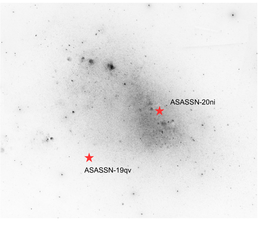
Figure 1: The DSS2 image of the SMC obtained by the Anglo-Australian Observatory (AAO) with the UK Schmidt Telescope. The positions of the two novae are marked with a red star.

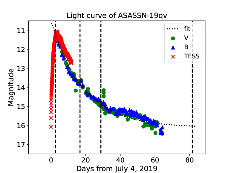
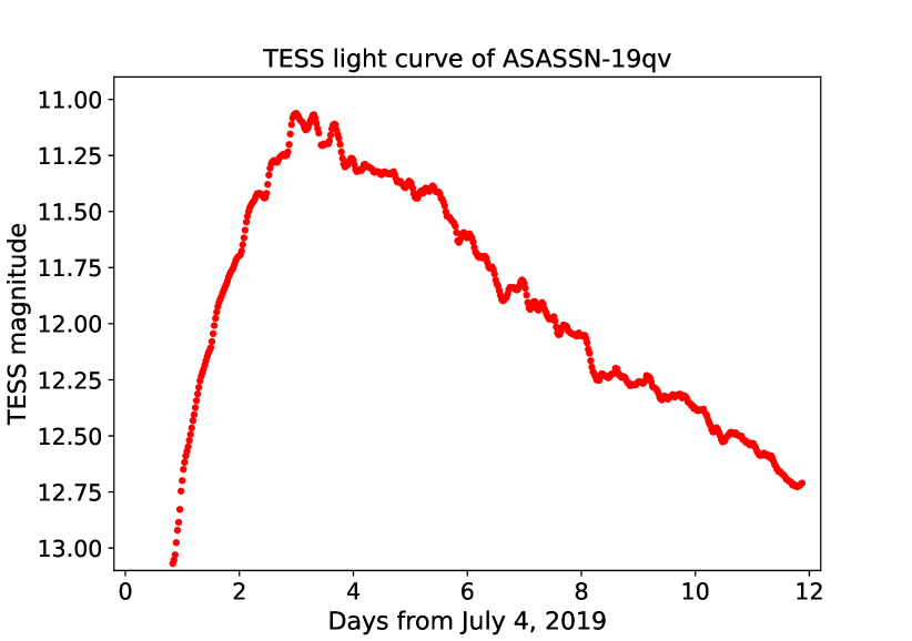
Figure 2: (Left panel) The light curve of ASASSN-19qv as obtained from the AAVSO data archive (Kafka, 2021) in the $B$ and $V$ filters and using the early TESS data, as described in the text. Dashed lines correspond to the spectral epochs presented in this work. The dotted curve represents the best-fit that we have found using an exponential decay function. (Right panel) An in-depth view of TESS data. The light curve shows small fluctuations in magnitude with amplitude of 0.1-0.2 mag.

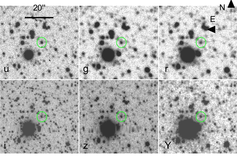
Figure 4: Multi-images of the field of view around ASASSN-19qv as observed in the $ugriz$-bands by the SMASH survey (Nidever et al., 2017) and in the $Y$-band as observed by the VISTA Magellanic Cloud survey (Cioni et al., 2011). The position of the nova is marked with a green circle and it shows the counterpart reported in the text.

The classical nova ASASSSN-19qv was discovered by the ASAS-SN survey (Shappee et al., 2014) on July 4, 2019 as a new transient of $g$ = 14.2 mag in the direction of the SMC as shown in Fig. 1. There is a source in the Gaia DR2 (ID 4685624636344633728) at the position of the nova for which the reported parallax is negative, suggesting a very distant object, in agreement with being as distant as the SMC. The Gaia $G$ magnitude for this source is $G=20.68$ mag. The field of view of ASASSN-19qv was observed by the SMASH survey (Nidever et al., 2017) in the $ugriz$ filters. There is a source at the position of ASASSN-19qv in all the filter images, which is slightly extended toward the NE direction, suggesting that this source is actually composed by two stars. Using nearby stars taken from the USNO B1 catalog we measure a magnitude for this source of $i=20.0\pm 0.5$ mag. We have also found a catalog photographic magnitude of $B_{j}=20.65$ in the Guide Star Catalog release 2.3 (Bucciarelli et al., 2008) for the source reported at the position of the nova. Additionally, the field of view of ASASSN-19qv was covered by the VISTA Magellanic Cloud survey (Cioni et al., 2011) on Aug 16, 2014. One source in the Y-band is coincident with the position reported for ASASSN-19qv, see fig. 4, for which we determine $Y=21.3$ mag. However, the double nature of the SMASH source suggests that it could be a foreground faint Galactic star or possibly red giant in the SMC. High-resolution imaging combined with spectroscopic observations of this source during the quiescence phase will definitely reveal the real nature of the progenitor.

A first spectrum obtained two days after the discovery of the nova confirmed the transient as a classical nova thanks to the identification of P-Cygni lines of Fe ii, O i and Na i in addition to Balmer lines, with expanding blue-shifted velocities of $\sim$ -900, -1000 km/s (Aydi et al., 2019). Spectroscopic observations obtained in the following days (Days 5 and 8, Bohlsen, 2019a, b) still showed the presence of Fe ii absorption lines and the absence of higher ionization transition like He i. We started to observe ASASSN-19qv with the UVES spectrograph at ESO Very Large Telescope (Program ID: 2103.D-5044, PI Izzo) after 16 days from discovery. The wavelength range covered by UVES starts from 310 nm to 950 nm at a spectral resolution of $R=40,000$. The following two epochs, Day 29 and Day 81, were obtained with X-shooter at ESO/VLT, covering a wider spectral range from 300 nm to 2500 nm and with a resolution variable from $R=6,700$ for the VIS and NIR arms to $R=8,900$ for the UVB arm. The detailed log of the observations is shown in Table 1.

2.2 ASASSN-20ni

ASASSN-20ni was also discovered by the ASAS-SN survey on October 26, 2020 as a new transient of $g$ $\sim$ 14.1 mag and was confirmed the following day when it increased in brightness to $g$ $\sim$ 12.2 mag (Way et al., 2020). The ASAS-SN survey also monitored the position of the sky where ASASSN-20ni was located in the previous six years, and no previous outburst from the nova progenitor brighter than $g>$ 16.5 mag were reported.

We searched for the possible presence of the nova progenitor in archival data surveys. To improve the astrometry from ASAS-SN we used the UVES acquisition image to calibrate astrometry at sub-arcsecond precision. No clear sources have been found in the SMASH survey and in the VISTA Magellanic Cloud survey down to a magnitude limit of Y $>$ 21.5 mag, despite the nova being 2 arcsec from a bright ($Y$ = 17.8 mag) star and 1.5 arcsec from another fainter source, see also Fig. 5.

The day following the discovery ASASSN-20ni was classified as a Fe ii nova using the Goodman spectrograph covering the wavelength range between 620 and 720 nm (Aydi et al., 2020). The spectrum was characterised by P-Cygni emission line profiles for Balmer, Fe and N lines with absorption trough minimum at $v_{exp}\sim-500$ km/s. We started to observe ASASSN-20ni with the UVES spectrograph using a dedicated Discretional Director Time program (Program ID: 2106.D-5008(B), PI Izzo) four days after the nova discovery. We used different exposure times for the different UVES arms and dichroic configurations, in order to optimize the signal-to-noise in the near-UV range and at the same time avoid possible saturation from bright lines between 480 and 850 nm. The log of the observations is shown in Table 1.

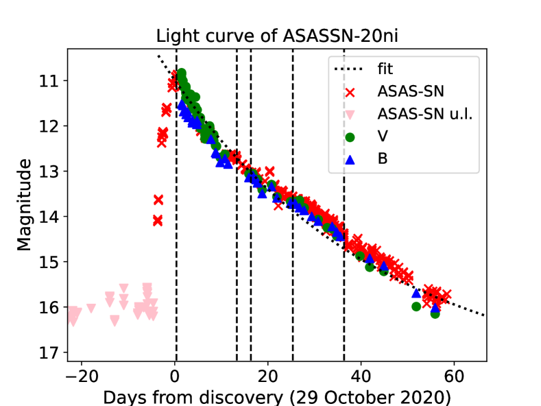
Figure 3: The light curve of ASASSN-20ni as obtained from the AAVSO data archive (Kafka, 2021) in the $B$ and $V$ filters and using the ASAS-sn $g$ filter data, as described in the text. Dashed lines correspond to the spectral epochs presented in this work. The dotted curve represents the best-fit found using an exponential decay function.

For both novae we reduced the UVES and X-Shooter data using a pre-compiled pipeline based on the python-cpl libraries, which make use of the standard ESO Recipe Execution Tool (esorex).

Table 1: Log of the observations.

Epoch	Instrument	Exp. time	Wav. range	Resolution $R$
(Day)		$(s)$	$(nm)$	$(\lambda/\delta\lambda)$
ASASSN-19qv
2	Goodman	1x500	400-800	$\sim$1,850
16	UVES	3x900 & 3x300	310-945	40,000
29	X-shooter	2x600 & 2x300	300-2,500	6,700-8,900
81	X-shooter	2x600 & 2x300	300-2,500	6,700-8,900
ASASSN-20ni
4	UVES	1x1800 & 3x900	310-945	$\sim$1,850
17	UVES	2x600	380-945	40,000
20	UVES	1x2200 & 2x600	310-945	40,000
29	UVES	1x2200 & 3x600	310-945	6,700-8,900
40	UVES	1x1800 & 2x900	310-945	6,700-8,900

3 Data Analysis

3.1 ASASSN-19qv

The light curve of ASASSN-19qv was obtained using AAVSO (Kafka, 2021) data and TESS public data. TESS data cover the range between 600 and 1000 nm with a very high temporal sampling. At a cadence of 0.5 hour cadence, they reveal presence of fluctuations with amplitude of 0.1-0.2 mag on a timescale of a few hours, see Fig. 2. There is a lack of data after $\sim$ 60 days from the nova discovery. The $V$-band early evolution is well modelled as an exponential decay with constant decay $b=0.05$ mag/days. The best-fit with such a function provides also an estimate for the $t_{2}$ value, which results to be $t_{2}=11.0$ days, implying that ASASSN-19qv is close to being classified as a fast nova, according to the classification of Payne-Gaposchkin (1957).

The high-resolution spectrum provided by UVES allows us to identify SMC interstellar lines, like Ca ii H,K lines, and then to determine the velocity offset due to the motion of the SMC that will be considered in the analysis presented in this work. In Fig. 6 we show the heliocentric radial velocity of both Ca ii IS lines, in addition to the Na i D2 line. While Na i is almost absent in the SMC environment, the Ca ii lines are clearly detected and they are characterised by a main absorption centered at $v_{SMC,1}=130$ km/s, which will be considered as the main SMC offset in the rest of the analysis for this nova. We also note a narrow component at lower velocities, $v_{SMC,2}=90$ km/s likely due to an additional cloud of interstellar gas in the SMC along our line of sight.

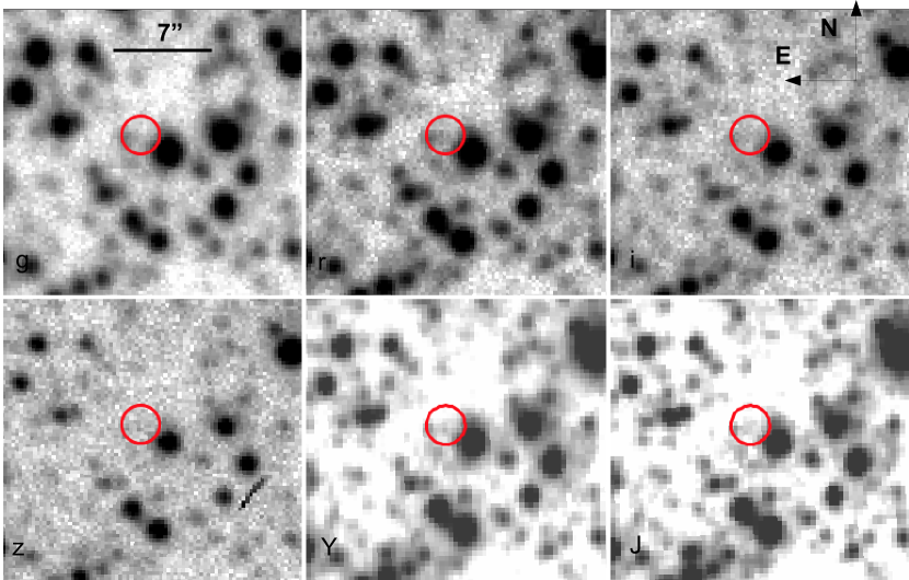
Figure 5: Multi-images of the field of view around ASASSN-20ni as observed in the $griz$-bands by the SMASH survey (Nidever et al., 2017) and in the $YJ$-bands as observed by the VISTA Magellanic Cloud survey (Cioni et al., 2011). The position of the nova calibrated with the UVES acquisition image is marked with a red circle.

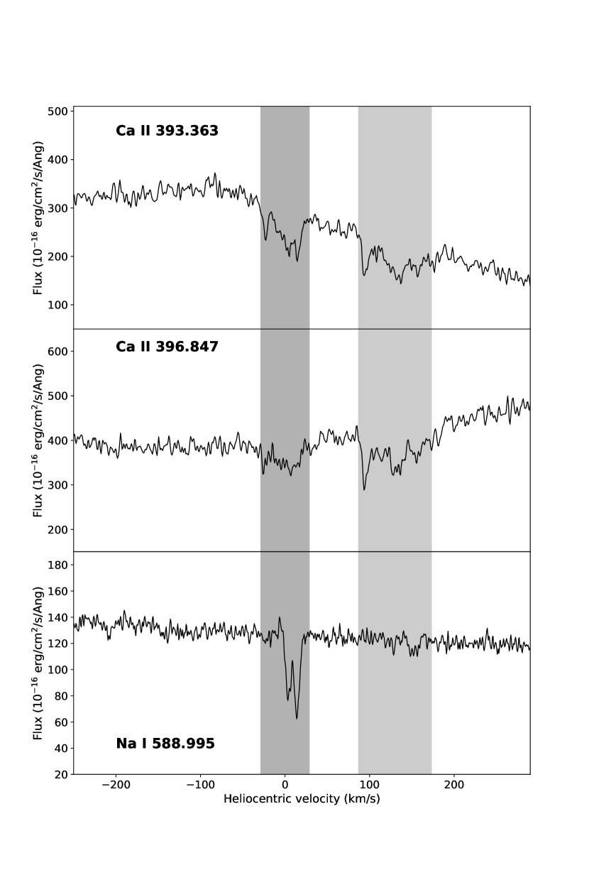
Figure 6: The Day 16 spectrum of ASASSN-19qv centered around the Ca ii $\lambda$393.3 (upper panel), the Ca ii $\lambda$396.8 lines (middle panel) and around the Na i $\lambda$588.995 nm IS line (lower panel). Velocities are corrected for the heliocentric correction. The SMC interstellar Ca ii absorptions are observed at $v_{SMC}=+130km/s$ and are broader than the corresponding Milky Way (MW) lines. These are marked with a light gray strip, while the MW component is reported with a darker strip.

3.1.1 The spectroscopic evolution

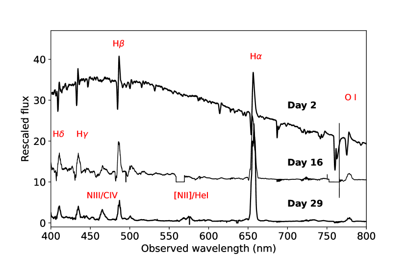
Figure 7: Spectral evolution of the nova ASASSN-19qv in the first month after the discovery. Spectra have been rescaled in flux and shown in the range (400, 800) nm. The presence of helium, blended with Fe ii, nitrogen lines and of a bright Bowen blend at 464.0 nm observed in the Day 16 spectrum marks the transition from the Fe ii to the He/N type, classifying this nova as a hybrid case, according to Williams (1994). In the Day 29 spectrum, the presence of a rising [N ii] 575.5 nm line marks the transition to the ”auroral” phase.

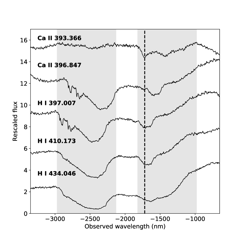
Figure 8: Day 16 spectrum of ASASSN-19qv, corrected for the SMC motion, showing the P-Cygni absorptions of Ca ii H,K lines and Balmer H$\gamma$, H$\delta$ and H$\epsilon$ lines. The absorption components are clearly visible in all Balmer lines. The Ca ii 396.847 nm is blended in the broad P-Cygni of H$\epsilon$ and only the prominent feature at $v=-1720$ km/s is clearly visible (the dashed black line). The high velocity component in the Ca ii 393.366 nm line is less pronounced, suggesting a very low density for the Calcium in this component.

Our first spectrum covers the 400 – 800 nm range and was observed only two days after discovery. It is characterised by the presence of Balmer, Na i and Fe ii P-Cygni absorption lines with blue-shifted absorption velocities between $-$900 and $-$1,000 km/s. The O i $\lambda$777.5 nm line is the brightest non-Balmer line, implying that this spectrum is typical of the Fe ii nova spectral class, see also Fig. 7.

The second spectrum obtained 16 days after the nova discovery peaks at bluer wavelengths than the first spectrum. It shows P-Cygni profiles for Balmer lines characterised by two main absorption components, at the blue-shifted velocities of $v_{1,a}=-1,710$ km/s and $v_{1,b}=-2,400$ km/s. The brightest non-Balmer line is O i $\lambda$844.6 nm. The Fe ii $\lambda$516.9nm line now shows fainter P-Cygni absorptions at the same velocities of the Balmer lines, indicating that the ionization state is increasing. This evidence is also confirmed by the presence of faint, but emerging, He i lines, in particular the He i $\lambda$501.6 nm line that is blended with Fe ii $\lambda$501.8 nm, and the presence of N i and C ii lines. The third spectrum (Day 29) shows higher ionization transitions like the Bowen (N iii-C iv) blend at 464.0 nm in addition to a rising [N ii] $\lambda$575.5 nm line, which mark the beginning of the ”auroral” phase. In the near-IR range the brightest line, with the exception for the Paschen-$\alpha$, is O i $\lambda$1128.7 nm as it is expected given the high luminosity of the O i $\lambda$844.6 nm line. This evidence suggests that the photo-excitation by accidental resonance (Kastner & Bhatia, 1995) is still working at this epoch. The ratio $R_{\text{O\,{i}}}$ between O i $\lambda$844.6 nm / O i $\lambda$777.5 nm has been proposed by Williams (2012) as a density diagnostic for the ejecta. We measure $R_{\text{O\,{i}},1}=3.5$ in the Day 14 spectrum and $R_{\text{O\,{i}},1}=12.6$ in the Day 27 spectrum, suggesting a relatively high density of the ejecta, more similar to Fe ii-type novae, but rapidly decreasing between the two epochs.

The wavelength range of the spectra obtained with UVES and X-shooter extends to the near-UV part of the electromagnetic spectrum, permitting to analyse with a good signal-to-noise the region where the resonance transition of the ⁷Be ii $\lambda$ 313.0/1 nm doublet isotope falls. Indeed, in both early epochs (Day 14 and Day 27) we detect blue-shifted absorption components that we have identified as due to the ⁷Be ii $\lambda$ 313.0/1 nm transition, see also Figs. 8, 12. In the Day 14 spectrum we clearly see two broad P-Cygni absorptions that share the same expanding velocities of the P-Cygni absorptions observed in Balmer lines, as well as in other transition as O i. These absorption components are characterised by expanding velocities of $v_{Day16,1}=-1,630$ km/s and $v_{Day16,2}=-2,400$ km/s as observed in the Day 14 spectrum, with the slow component being less intense than the fast one. This difference is more clear in the spectrum obtained on Day 27, where the slow expanding component, with a measured velocity of $v_{Day29,1}=-1,790$ km/s, becomes more narrow while the fast component is characterised by a broad profile ($FWHM_{H\beta}\approx 900$ km/s) centered at the value of $v_{Day29,2}=-2,600$ km/s. This behavior is observed in all the main Balmer lines as well as in the ⁷Be ii $\lambda$ 313.0/1 nm transition. This is the main evidence that beryllium was synthesized during the TNR preceding the outburst of ASASSN-19qv.

The Day 81 spectrum shows the absence of high-velocity blue-shifted absorption features, observed in the previous epochs, but we still detect permitted transitions like O i 844.6 nm (including the 1129.1 nm in the near-IR range), and the flux ratio with the O i 777.5 nm which is blended with [Ar iii] is now $R_{\text{O\,{i}}}=8.1$, suggesting an environment still relatively dense. There are also high-ionization lines such as He i ground state transitions 1,008.3/2,005.8 nm as well as excited transitions (587.6/706.5 nm lines among the many others barely discernible in the spectrum). We also detect the presence of typical forbidden transitions observed in the nebular phase of classical novae like the [O iii] 436.3/495.9/500.7 nm, the [N ii] 575.5 nm, suggesting that the physical conditions of the ejecta at this stage are very heterogeneous (see Fig. 14). Then we can not use this spectrum to infer physical properties like the density, temperature and the hydrogen mass of the ejecta. We do not detect forbidden neon lines at this epoch, suggesting a CO-type WD for the nova progenitor.

3.2 ASASSN-20ni

The light curve of ASASSN-20ni was built using AAVSO data (Kafka, 2021). We have also used ASAS-SN $g$-band data that covers the rising phase of the nova and its decay up to $\sim$ 60 days after the peak brightness, see Fig. 3. The last non-detection from the ASAS-SN survey was dated October 25, 2020, e.g. one day before the first nova detection by the same project (Way et al., 2020). The light curve evolution in the first 60 days of the nova emission can be modelled using an exponential function, despite the light curve showing a short rebrightening at $\sim$ 20 days from the peak brightness. Using the AAVSO $V$-band data, we measure a decay rate of $b=0.02$ mag/days, and a $t_{2}$ parameter of $t_{2}=17.4$ days, which classify ASASSN-20ni as a fast nova.

ASASSN-20ni was observed in the central region of the SMC, whereas ASASSN-19qv was located at a more peripheral region, see Fig. 1. This is reflected on the amount of gas surrounding the nova location as inferred from the analysis of interstellar lines. As observed in the Ca ii H,K lines, we note multiple components at $v_{SMC}$ = 105, 131, 156 and 194 km/s, with the latter being the most intense component, see also Fig. 9. Similar to the spectrum of ASASSN-19qv, the Na i inter-stellar component is less pronounced, showing only the components at $v_{SMC}$ = 105 and 194 km/s. In the following, we will consider the highest velocity component at $v_{SMC}$ = 194 km/s as our reference to correct all our spectral series to the SMC velocity.

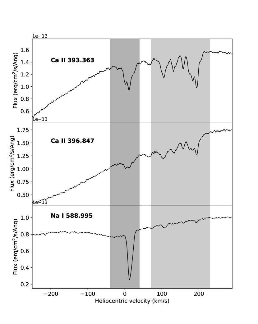
Figure 9: The Day 4 spectrum of ASASSN-20ni centered around the Ca ii $\lambda$393.3 (upper panel), the Ca ii $\lambda$396.8 lines (middle panel) and around the Na i $\lambda$588.995 nm IS line (lower panel). Velocities are corrected for the heliocentric correction. The SMC interstellar Ca ii absorptions are observed at multiple velocity (see text).

3.2.1 The spectroscopic evolution

The first spectrum of ASASSN-20ni was obtained just four days after its discovery. It shows a very optically thick continuum, typical of the Fe ii spectral class (Williams et al., 1991), and is characterised by the presence of a ”forest” of absorption lines in the range between 300 and 550 nm, see also Fig. 10. After re-scaling the spectrum at the SMC velocity assumed for this nova, we measure blue-shifted absorption velocities of $v_{exp}$ $\sim$ -520 km/s for Na i, Ca ii, and Fe ii lines, while Balmer lines show a broader absorption trough extending to higher velocities. We also detect at the same expanding velocity the majority of THEA lines listed in Table 2 of Williams et al. (2008), with the exception of V ii lines. We cannot clearly confirm the presence of Li i 670.7nm, despite broad absorption being observed at the corresponding blue-shifted wavelength.

The second spectrum, obtained two weeks later (Day 17), and covering the range from 375 to 500 nm and from 580 to 946 nm, shows an evolved spectrum where almost all THEA lines have disappeared. The brightest non-Balmer line is O i 844.6 nm, showing a main P-Cygni absorption system at higher velocities $v_{exp}$ = -700 km/s, similar to what is measured for Balmer and Fe ii lines. Interestingly, the Na i doublet shows a more structured profile, with signatures of two components at velocities of $v_{1}=-650$ km/s and $v_{2}=-520$ km/s. This velocity configuration for the ejecta is also observed in the following spectra (Day 20 and Day 29). At these epochs, bright emission lines display a saddle-shaped profile with the two bright peaks at $\pm\sim$ 500 km/s, which suggests an asymmetric geometry for the nova ejecta (Mukai & Sokoloski, 2019). The last spectrum obtained on Day 40 still presents low-ionization transitions such as the Fe ii multiplet 42, but we also see enhanced higher-ionization transitions such as the Bowen blend in emission and the He i 587.5 nm, which was identified by the presence of a P-Cygni absorption with blue-shifted velocity of $\sim$ -650 km/s. Interestingly, lower ionization transitions such as Ca ii, Fe ii and Na i show a more intense lower velocity ($\sim$ -520 km/s) component over-imposed to the higher velocity component with intensity fading with the increasing velocity to -700 km/s, see Fig. 11.

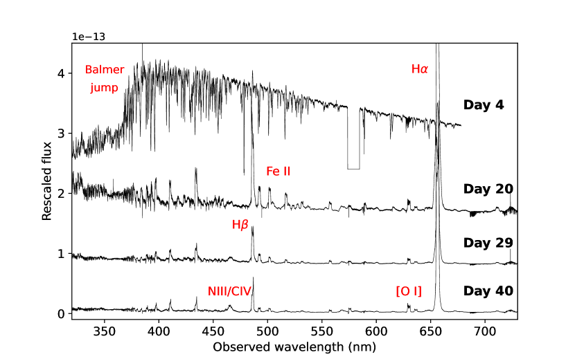
Figure 10: Spectral evolution of the nova ASASSN-19qv in the first 40 days after the discovery. Spectra have been rescaled in flux and shown in the range (330, 740) nm.

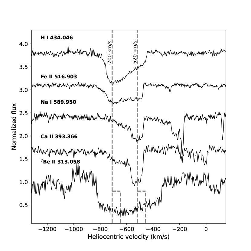
Figure 11: The Day 40 spectrum of ASASSN-20ni, corrected for the SMC motion, showing the P-Cygni absorptions of Ca ii K, H$\gamma$, Fe ii 516.9 nm, Na i 589.9 nm and of ⁷Be ii 313.0 nm lines. The plot shows the different profile of Ca ii and Na i, which show a prominent absorption at -530 km/s and a more faint high-velocity tail, with respect to H i, Fe ii and ⁷Be ii lines where the higher velocity component centered at $\sim$ -700 km/s and extending to -800 km/s is more pronounced. This evidence suggests a different abundance composition for the two components and supports a two-ejecta component scenario (Mukai & Sokoloski, 2019). for the ⁷Be ii line are reported the expected positions of the two doublet components.

4 Abundance of ⁷Be

4.1 ASASSN-19qv

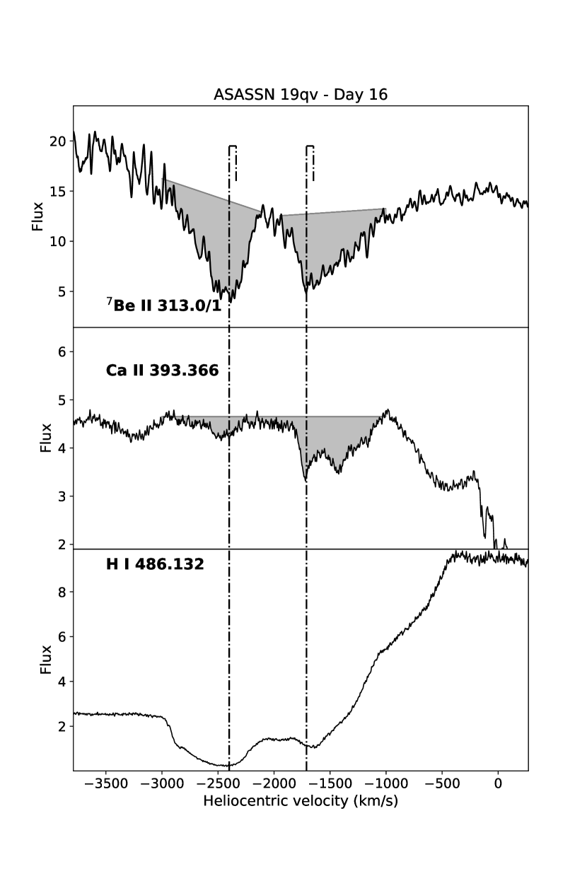
Figure 12: The Day 16 spectrum of ASASSN-19qv, corrected for the SMC motion, showing the P-Cygni absorptions of the ⁷Be ii $\lambda$313.0 at blue-shifted velocities of $v_{1a}$ = -1710 km/s and $v_{1b}$ = -2400 km/s and compared with the Ca ii $\lambda$396.8 and with H$\beta$ . The dashed regions mark the area of the absorptions considered for the EW estimate.

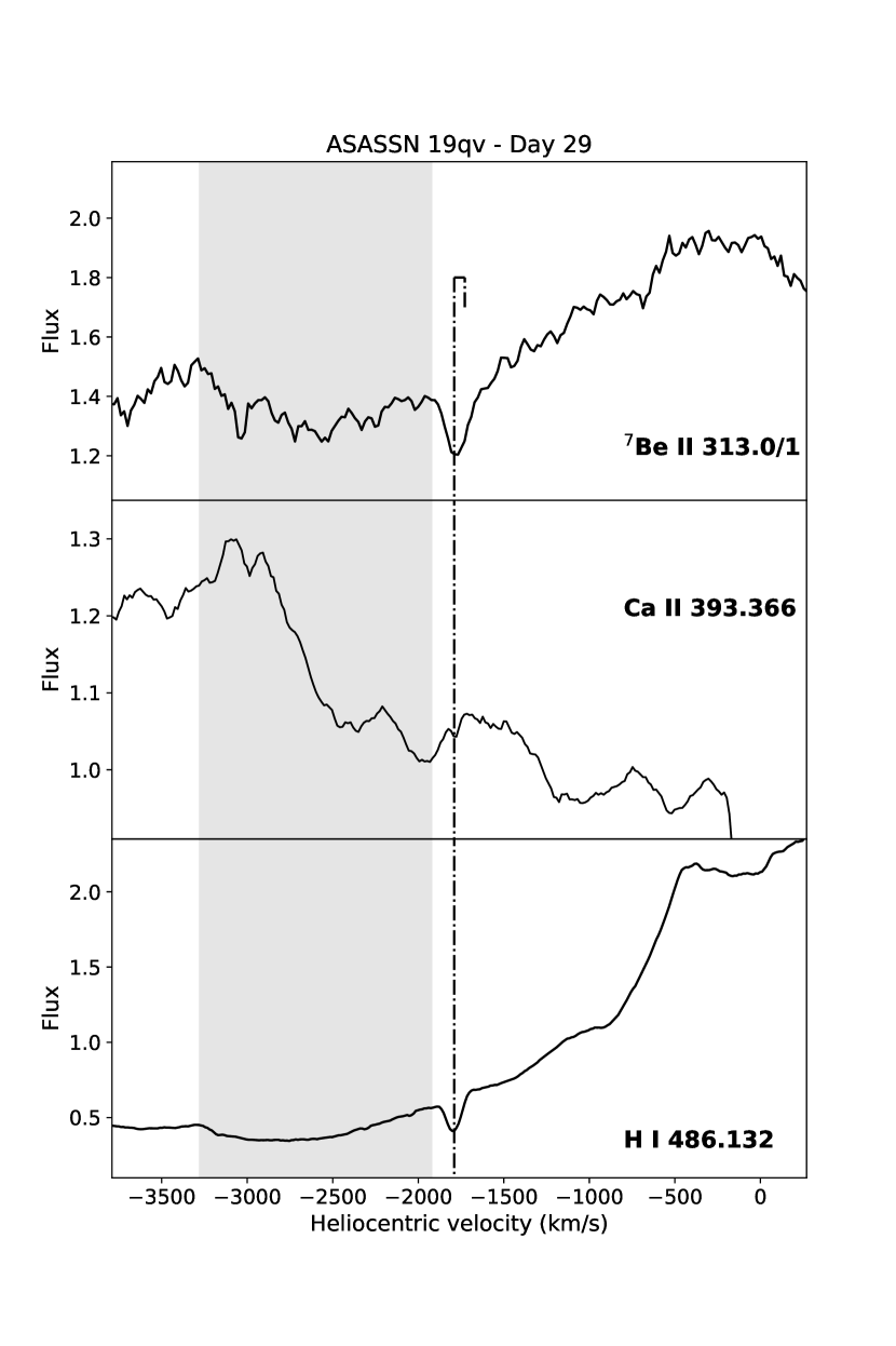
Figure 13: The Day 29 spectrum of ASASSN-19qv, corrected for the SMC motion, showing the P-Cygni absorptions of the ⁷Be ii $\lambda$313.0, the Ca ii $\lambda$396.8 and with H$\beta$ at blue-shifted velocities of $v_{1a}$ = -1710 km/s, while the gray dashed region indicates the broad component centered at $v_{1b}$ = -2600 km/s.

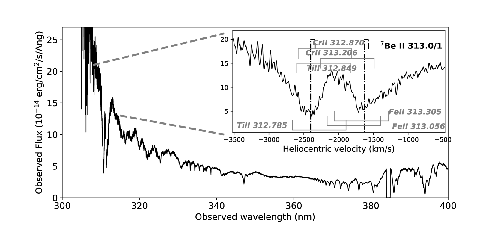
Figure 14: The Day 16 spectrum of ASASSN-19qv in the region 300-400 nm. The inset plot shows the region centered around the Be ii $\lambda$313.058, which shows the expected positions of low ionisation transition absorptions of Cr ii, Ti ii and Fe ii. Velocities are corrected for the heliocentric correction.

Following Tajitsu et al. (2015) we quantified the amount of beryllium ejected in the ASASSN-19qv outburst by comparing the observed equivalent widths (EW) of the blue-shifted absorption components with the EW of a reference element. The resonance lines of ionised calcium Ca ii $\lambda\lambda$393.4/396.8 nm H,K are the more suitable, given that calcium shares the same configuration of their outermost electron shells. A detailed analysis of Day 16 spectrum shows the presence of faint blue-shifted components for the Ca ii 393.4 nm line centered at the same velocities observed for the Balmer lines, see Fig. 8.

The other doublet component, Ca ii 396.8 nm, is blended within the P-Cygni of the H i 397.0 nm line, but we confirm its presence through the identification of a faint feature corresponding to the main absorption observed for all transitions at $v=-1,720$ km/s. Moreover, we observe that the high-velocity absorption components of Calcium lines are much fainter when compared with the slower components, while for ⁷Be ii and Balmer lines this is not observed. This evidence suggests that the high-velocity component ejecta has a distinct element abundance. This difference can be explained in the case that high-velocity components arise from a distinct ejecta event, like the one proposed in Mukai & Sokoloski (2019), where a later fast wind-like, and likely bi-polar ejection is observed after the first phenomenon, which is slower and characterized by an oblated geometrical distribution. We will come back to this point later. In the spectrum obtained on Day 29, Ca ii lines almost disappeared. In the Day 29 spectrum we observed a very faint absorption for Ca ii 393.3 nm line, see Fig. 12, and in order to estimate the beryllium abundance we consider the analysis of the UVES Day 16 spectrum.

Table 2: A list of single-ionized ions which are the main contributors to the absorption in the region around $\lambda$313.058 and that are shown in Fig. 14. Atomic data taken from the NIST lines data base. Those for Cr ii are from Lawler et al. (2017).

Wavelength (Air)	ion	Log(gf)	Low en.	Upper en.
nm			(eV)	(eV)
312.7850	Ti ii	0.15	3.87	7.83
312.8483	Ti ii	0.11	3.90	7.87
312.8700	Cr ii	-0.53	2.43	6.40
313.0565	Fe ii	–	3.77	7.73
313.2057	Cr ii	0.43	2.48	6.44
313.3048	Fe ii	-1.9	3.89	7.84

We have then measured the EWs for the ⁷Be ii and the Ca ii 393.4 nm for the blue-shifted absorption area as shown in Fig. 12. However, as also reported in our previous analysis (Molaro et al., 2020a), the absorption of ⁷Be ii is generally contaminated by the presence of low ionisation transitions of Cr ii, Ti ii and Fe ii. We have then analysed the presence of the most intense transitions (see Table 2) that fall close to the wavelength range of ⁷Be ii and in Fig. 14 we report their expected position in the spectral region surrounding the blue-shifted beryllium absorptions. We cannot clearly confirm the presence of Cr ii and Ti ii, given the relatively low signal-to-noise ($\sim$10) of the UVES spectrum around the ⁷Be ii transitions. We have also checked for the presence of absorption lines from the other transitions of these same elements originating from their parent multiplets, but it is hard to firmly establish their presence. We find possible evidence of the presence of Fe ii lines $\lambda\lambda$313.305,313.056, and other transitions arising from the same initial level like Fe ii $\lambda$316.794,314.472, whose detection, in addition to the already confirmed presence of Fe ii $\lambda$516.903, confirms the presence of iron in the ejecta of ASASSN-19qv. Consequently, in our final estimates of the ⁷Be ii EWs, we are taking into account the presence of these line blends.

Our final results are shown in Table 3, where we report the measured EWs for the low and high velocity components, as well as the total value. The EW ratio between ⁷Be and Ca for low velocity component, EW(⁷Be ii_low)/EW(Ca ii_low) = 2.26 $\pm$ 0.07, while for the high velocity component we measure a much higher value, namely EW(⁷Be ii_high)/EW(Ca ii_high) = 8.58$\pm$0.07. In the following analysis we will not distinguish between these two emission components, given that both systems are escaping the binary and will then enrich the ISM of the SMC. But, a detailed analysis included in a wider context is needed and will be presented elsewhere. For the entire absorption systems we consider the average ratio between the two components, obtaining EW(⁷Be ii)/EW(Ca ii) = 3.50$\pm$0.09. This value slightly exceeds the mean value of $\sim 1.5\pm 0.2$ found in Galactic novae (Molaro et al., 2020a). Following Spitzer (1998), the relative number abundance can be inferred from:

$$\frac{N(^{7}\text{Be\,{ii}})}{N(\text{Ca\,{ii}})}=2.164\times\frac{EW(^{7}\text{Be\,{ii}})}{EW(\text{Ca\,{ii}})}$$ (1)

⁷Be ii is unstable with an half-life time decay of $t_{1/2}=53.3$ days. Thus, considering the correction factor of $K=1.23$ we obtain N(⁷Be ii) = (9.32$\pm$0.30) $\times$ N(Ca ii).

Table 3: Equivalent width measurements for the ⁷Be ii and Ca ii 393.4 nm blue-shifted absorptions in the Day 16 spectrum of ASASSN-19qv.

Day	EW(7Be iilow)	EW(7Be iihigh)	EW(7Be iitot)	EW(Ca iilow)	EW(Ca iihigh)	EW(Ca iitot)
	(Å)	(Å)	(Å)	(Å)	(Å)	(Å)
16	3.32$\pm$0.05	3.09$\pm$0.07	6.41$\pm$0.09	1.47$\pm$0.01	0.36$\pm$0.02	1.83$\pm$0.02

4.2 ASASSN-20ni

The velocity distribution of the ejecta along the evolution of the outburst is crucial to identify the presence of features due to the doublet resonance lines of ⁷Be ii. In Fig. 15 the evolution of the region between 310 and 314 nm is shown to highlight the presence of a broad absorption around $\sim$ 312.5 nm. This absorption corresponds to ⁷Be ii 313.0/1 nm and matches the blue-shifted velocities reported for other ions observed in the spectrum at the same epoch.

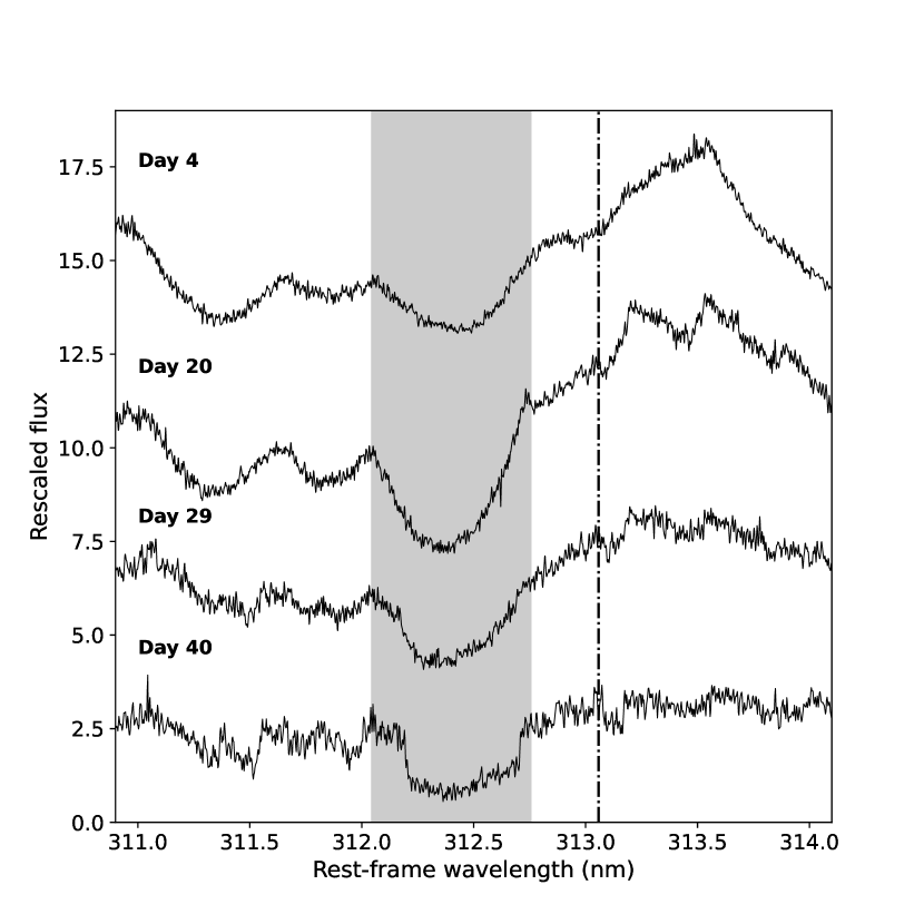
Figure 15: The evolution of the broad absorption feature centered at $\lambda$ = 312.5 nm, marked with a gray shaded region, and attributed to ⁷Be ii 313.0/1 nm doublet. The dot-dashed black line marks the rest-frame position of the ⁷Be ii 313.0 nm line.

Unfortunately, our spectral observations cover the first 40 days only, such that we could not follow-up the evolution of the ⁷Be P-Cygni profile until narrow features would appear, as due to the expanding ejecta and its consequent density decay, similar to the case of ASASSN-19qv previously discussed. Moreover, in ASASSN-20ni we could not disentangle the low and high velocity components, being apparently embedded in the observed absorption profile, see Fig. 11. Consequently, we have done a careful measurement of the EW of the total absorption profile, paying attention to the contribution of other lines, such as Fe ii, Ti ii and Cr ii (see the list on Table 2), similarly to what was done for ASASSN-19qv. The presence of THEA lines in the early spectra of ASASSN-20ni represents important information for our analysis: we already know their expanding velocities which corresponds to the lower velocity component, and then their position in the spectrum.

In Table 4 we report on our final measurement of the EW of the ⁷Be ii 313.0/1 nm blue-shifted absorption, as well as of Ca ii 393.3 nm, which we will use as our reference for the estimate of the Be abundance, as already discussed in Section 4. The EW ratio between ⁷Be and Ca is EW(⁷Be ii)/EW(Ca ii) = 2.14$\pm$0.24, as estimated from the Day 40 spectrum. Assuming a correction factor of $K=2.11$ for the ⁷Be ii decay, finally we obtain N(⁷Be ii) = (9.81$\pm$0.52) $\times$ N(Ca ii), which is in good agreement with the Be abundance value estimated for ASASSN-19qv.

Table 4: Equivalent width measurements for the ⁷Be ii and Ca ii 393.4 nm blue-shifted absorptions in the Day 20, 29 and 40 of ASASSN-20ni.

Day	EW(7Be iitot)	EW(Ca iitot)
	(Å)	(Å)
20	2.45 $\pm$ 0.11	2.58 $\pm$ 0.11
29	2.19 $\pm$ 0.12	2.09 $\pm$ 0.13
40	2.77 $\pm$ 0.18	1.29 $\pm$ 0.12

5 Discussion

5.1 ⁷Be (=⁷Li) yields

From our previous analysis we infer an average beryllium abundance of N(⁷Be ii) = (9.63$\pm$0.50) $\times$ N(Ca ii). Following similar studies (Molaro et al., 2022), we assume that singly ionized ions of Be ii and Ca ii represent the main ionization stage for the ejecta and calcium is not produced in the nova explosion. Calcium can be also synthesised in massive oxygen-neon WDs where the peak temperatures can reach very high values ($T\sim 5\times 10^{8}$ K and more). Some observations have indeed reported Ca abundance values in nova ejecta up to one order of magnitude larger than the Solar value (Andrea et al., 1994) suggesting a possible production channel for heavy ($A\sim 40$) elements in very hot WDs (Christian et al., 2018; Setoodehnia et al., 2018). The lack of neon in ASASSN-19qv suggests that the progenitor WD of ASASSN-19qv is not an extremely, hot massive WD. For ASASSN-20ni, unfortunately, due to the lack of late-time spectra, we could not verify the presence of bright forbidden neon lines in the near-UV, which would imply a ONe underlying WD. However, the larger $t_{2}$ value suggests a similar, if not lower, massive WD progenitor. On the other hand, Starrfield et al. (2020) found that a large over-production of ⁴⁰Ca (up to ten times the Solar value) is obtained from their 1D hydrodynamic simulations of the TNR in CO novae. An increase in ⁴⁰Ca abundance would lead to a corresponding increase on the ⁷Be yield, with important consequences for the lithium enrichment of the SMC. However, measuring ${}^{40}Ca$ abundance in nova ejecta requires a high-cadence spectral coverage of the optically thick phases, when the ejecta is relatively cold, given the strong sensitivity of calcium ionization to the ambient temperature (Chugai & Kudryashov, 2020; Molaro et al., 2022). We therefore assume here that Ca in the ejecta shares the average value of the SMC stellar populations.

The mean stellar metallicity of the SMC is $[Fe/H]=-0.59\pm 0.06$, obtained from the analysis of massive and young OB stars (Trundle et al., 2007; Bouret et al., 2003; Korn et al., 2000). Recent measures from a large-scale photometric analysis of the SMC have reported an average value of $[Fe/H]=-0.95\pm 0.08$, using the slope of the Red Giant branch as an indicator of the metallicity (Choudhury et al., 2018). The location of ASASSN-19qv is, however, quite peripheral, while ASASSN-20ni is in the inner region of the SMC. Carrera et al. (2008) report a significant gradient with the metallicity decreasing toward the external regions. The inner part of the SMC is characterised by higher metallicity values ($[Fe/H]\sim-0.6$). The existence of two peaks at $[Fe/H]=-0.9/-1.0$ and at $[Fe/H]=-0.6$ in the metallicity distribution of the SMC was also reported in Mucciarelli (2014). In the following, we will use the value of $[Fe/H]=-0.6$ for both novae. Given that the solar abundance of calcium is N(Ca)/N(H)_⊙ = 2.2 $\times$ 10^-6 (Lodders et al., 2009), we obtain that the Ca abundance value in the SMC is N(Ca)/N(H)_SMC = (5.5 $\pm$ 0.4) $\times$ 10^-7. With this value we obtain a ⁷Be, or ⁷Li yield of N(⁷Li)/N(H) = (5.3 $\pm$ 0.2) $\times$ 10^-6.

We are not able to estimate the mass ejected directly but the two novae studied here are fast novae, which suggests high expansion velocities and lighter mass for the ejecta (Warner, 1989; Della Valle & Izzo, 2020). Uncertainty in the lithium yield is possible when considering that some Calcium could be in the form of Ca III. Chugai & Kudryashov (2020) suggested the possibility that some over-ionization could be present in the nova ejecta. This would lead to a decrease in the abundance of Ca ii with the consequence to over-estimate the total abundance of ⁷Be. Incidentally, this would alleviate the tension between observations and TNR theory (Starrfield et al., 2020). Molaro et al. (2022), using the photoionization code Cloudy (Ferland et al., 2017), showed that over-ionization in the ejecta of CNe is indeed possible but requires unlikely low densities and high temperatures of the gas. Moreover, the detection of neutral species transitions led them to conclude that the main ionization phase of calcium is the single-ionized stage. We have detected the Mg i 383.8 nm line at the same velocities of the expanding ejecta components of the two novae presented in this work, on Day 16 for ASASSN-190qv and on Day 20 for ASASSN-20ni, respectively. In the spectrum of ASASSN-20ni we also report the presence of Ca i 422.6 nm line, which suggests a low ionization stage for Calcium.

5.2 Historical novae in the LMC

Following these detections, we searched in the IUE archive for observations of classical novae exploded in the Magellanic Clouds with IUE, the International Ultraviolet Explorer (Boggess et al., 1978). IUE has already been shown suitable for a ⁷Be search (Selvelli et al., 2018). The LWP camera of the IUE satellite covered the wavelength range 200.0-320.0 nm and in its low resolution mode, IUE ($\Delta\lambda\approx 0.5$ nm), was suitable for checking the presence of a wide feature near 313.0 nm. Nova LMC 1991 and Nova LMC 1992 have been followed by IUE. Representative early spectra for these two novae are shown in Fig. 16. Both spectra exhibit a strong absorption feature shortward of $\lambda$313.0 nm that can be identified as the blue-shifted resonance doublet of singly-ionized ⁷Be ii.

We note that this feature can be only partially explained as a blend of common iron curtain absorption lines of singly ionized metals. Previous studies of galactic novae found only a minor contribution by singly-ionized metals i.e. Cr ii, Fe ii, and Ti ii to this feature (Tajitsu et al., 2015, 2016; Molaro et al., 2016; Selvelli et al., 2018), see also Fig. 14. A blending contribution which is expected to be even lower for Novae in the Large Magellanic Cloud owing to its low metallicity. Schwarz et al. (2001), and using PHOENIX model atmospheres, found that the best agreement between the observations and the synthetic spectra of Nova LMC 1991 requires a metallicity of Z = 0.1 Z_⊙. This is a significantly lower metallicity than the canonical LMC value of $\sim$ 1/3 solar and lends stronger support to the identification of the $\lambda$313.0 nm feature as ⁷Be ii.

Beryllium and magnesium have similar ionization potentials and a rough estimate of the their relative abundances can be derived from the ratio of the EWs of their resonance absorption doublets. The two lines show a similar velocity profiles at the same blue-shifted velocity, which indicates that the two features are produced under similar conditions. The observed absorption EW of Mg ii could be partially reduced by the presence of the emission component. Moreover, lines of singly-ionized elements, e.g Cr ii, Ti ii and Fe ii, contribute for 10 to 20 percent to the EW of the $\lambda$313.0 line. From the data shown in Fig. 16 we measure an EW ratio of about 4.2/11.5 = 0.37 in the LMC1991 nova and a ratio of 3.6/12.9 = 0.28 in LMC 1992 nova and we adopt an average ratio $W(313.0)/W(280.0)$ $\sim$ 0.30. In the optically thin regime, this ratio provides an estimate of the number of absorbers ($N_{i}$) through the common relation of $W\propto N_{i}\times f_{ij}\times\lambda^{2}$. Since $f_{ij}$(313.0)/$f_{ij}$(280.0)$\sim$0.5 the observed EW ratio provides $N_{i}(313.0)/N_{i}(280.0)=0.48$ Since the second ionization potentials of the two ions have similar values (i.e., 18.21 eV and 15.04 eV, respectively), similar ionization fractions are expected. Thus, the above derived ratio also provides an estimate of the total ⁷Be/Mg abundance. Assuming the magnesium abundance being 1/4 of the solar (similar to the value assumed for the SMC, see next Section), namely 9.08 $\times$ 10^-6 (Lodders, 2019), the ⁷Be ii  abundance relative to hydrogen is given by $N(^{7}Be)/N(H)=9.08\times 10^{-6}\times 0.48\sim 4.36\times 10^{-6}$, which is very close to the yields derived here for the novae of the Small Magellanic Cloud.

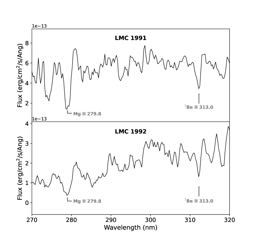
Figure 16: The IUE spectra of LMC 1991 (LWP20210LS, four days after the nova discovery) and LMC 1992 (LWP24303LL, $\sim$one day after the discovery) in the range 270.0-320.0 nm. The two strong absorption near 279.0 nm and 312.2 are identified as Mg II 280.0 and ⁷BeII 313.0 at the expanding blue-shifted velocity of $v_{exp}\sim-850$ km/s, assuming an expanding velocity for the LMC of $v_{LMC}=240$ km/s (McConnachie, 2012). Both spectra are corrected for reddening using E(B-V) = 0.15 mag, see Cassatella et al. (2002).

5.3 On the Li-enrichment in the SMC

Howk et al. (2012), from the detection of the Li i interstellar line along the line-of-sight of SK 143, derived N(⁷Li)/N(H) = (4.8 $\pm$ 1.8) $\times$ 10^-10 and an absolute Li abundance of A(Li) = 2.68 $\pm 0.16$, a value which is close to the level expected from the SBBN, when considering the CMB baryon density. Howk et al. (2012) concluded that the value measured in the SMC interstellar medium corresponds to the primordial with a negligible stellar post-BBN production.

On the other hand, the nova lithium yield estimated here suggests a non-negligible role of classical novae in the lithium enrichment of the SMC. The ⁷Be produced in SMC novae will enrich the ISM of the SMC with freshly-produced ⁷Li. The lithium yield inferred from the analysis of ASASSN-19qv and ASASSN-20ni is $M_{{}^{7}Li}=M_{{}^{7}Be}=(3.7\pm 0.6)\times 10^{-10}$ M_⊙. Assuming all SMC novae eject a similar amount of lithium into the ISM of the SMC we can have an approximate estimate of their contribution. For this purpose we need to know the nova rate in the SMC. This quantity was recently discussed by Della Valle & Izzo (2020). These authors found a robust lower limit for the SMC nova rate of 0.7 events per year, which is consistent with r = 0.9 $\pm$ 0.4 yr${-1}$, measured by Mróz et al. (2016). In the following we take the latter value of the rate as a constant over the age of the SMC. The oldest globular cluster (GC) in the SMC, NGC 121, is 2-3 Gyr younger than the oldest GCs in the Milky Way (Glatt et al., 2008), and the average age of stars in the outer regions of the SMC is of $t_{SMC}=10.6\pm 0.5$ Gyr (Dolphin et al., 2001). Considering a time delay of $\sim 2$ Gyr for the formation of a nova-progenitor WD system, we assume for the action of nova system in the SMC a time interval $\tau=8.6\pm 0.5$ Gyr. Thus, the total lithium production from classical novae amounts to:

$$M_{Li,n}=M_{{}^{7}Li}\,\times\,r\,\times\,\tau$$ (2)

which gives

$$M_{Li,n}=(3.7\pm 0.6)\times 10^{-10}\times 0.9\times(8.6\pm 0.5)\times 10^{9}=(2.8\pm 1.9)M_{\odot}$$ (3)

The uncertainties reported in the final estimate of $M_{Li,n}$ correspond to maximum errors.

This value can be compared with Li/H through the SMC mass. An estimate of the neutral hydrogen gas mass is $M_{HI}=4.2\times 10^{8}$ M_⊙ by means of the H i 21cm line observed with the Australian Telescope Compact Array radio telescope (Stanimirović et al., 2004). This value is also in agreement with the results from the Parkes H i survey, $M_{HI}=4.02\pm 0.08\times 10^{8}$ M_⊙ (Brüns et al., 2005). The additional contribution of the molecular hydrogen $H_{2}$ can been derived from the far-infrared maps provided by the Spitzer Survey of the SMC. Leroy et al. (2007) estimated a total mass of $M_{H_{2}}=3.2\times 10^{7}$ M_⊙. Adding this value twice to the neutral hydrogen mass we obtain a final value for the hydrogen mass of $M_{H}=(4.8\pm 0.2)\times 10^{8}$ M_⊙. The total mass accounting also for stars was estimated by McConnachie (2012) in 9.20 $\times 10^{8}$ M_⊙. Therefore, the atomic fraction Li/H in the SMC due to novae becomes N(⁷Li)/N(H) = (4.0 $\pm$ 1.5 ) $\times$ 10^-10, or A(Li) = 2.64, which suggests that a non-negligible fraction of the lithium observed in the SMC could be originated from classical nova explosions.

In Fig. 17 we present the lithium evolutionary curve for a detailed chemical model for the SMC. The model is similar to those of chemical evolution of dwarf spheroidal galaxies described in Lanfranchi et al. (2006) as well as for the Gaia-Enceladus dwarf galaxy described in Cescutti et al. (2020), the first model following the evolution of lithium in external galaxies (see also Matteucci et al., 2021 for more satellites of the Milky Way). Compared to our Galaxy, dwarf galaxies have lower star formation efficiencies and galactic winds that prevent to reach solar metallicities. In particular, our model for SMC follows the equations described in Cescutti et al. (2020) and it has an evolution that lasts 10 Gyr, a Gaussian infall law with a peak at 4 Gyr and sigma of 1 Gyr. The total mass surface density is 50 M_⊙/pc² with a star formation efficiency of 0.06 Gyr^-1. We assume a Galactic wind that starts after 7 Gyr, with a wind efficiency of 0.8 Gyr^-1, proportional to the gas still present in the galaxy. These chemical evolution parameters are fixed to reproduce the metallicity distribution function and the [$\alpha$/Fe] vs [Fe/H] trend observed in giant stars of the SMC by Mucciarelli (2014). For lithium, we consider the same nucleosynthetic channels considered in Cescutti & Molaro (2019). The Li production is mainly from novae, with a small contribution from production from AGB (Ventura & D’Antona, 2010). For the spallation production, we adopt the spallation rates which are empirically derived from beryllium observations in stars belonging to the Gaia-Enceladus dwarf galaxy, which, however, remains very similar to that of the Galaxy (Molaro et al., 2020b). In Gaia-Enceladus, the relation is

$$A(Be)=0.729(\pm 0.059)\,\times\,[Fe/H]+0.856(\pm 0.117)$$ (4)

The scaling of Li/Be $\approx$ 7.6 for spallation processes is adopted (Molaro et al., 1997) which provides at the SMC metallicity a value of A(Li) = 1.94 made by spallation processes only. The Li destruction due to astration in the stellar recycling is also taken into account. The model is shown for two different initial Li values, according to the SBBN+Planck nucleosynthesis of $A(^{7}Li)=2.72\pm 0.06$ (Cyburt et al., 2016), or the Spite plateau at A(Li) = 2.20$\pm$ 0.05. The present estimated values are A(Li) = 2.56 $\pm$ 0.04 when starting from the primordial value taken from the halo stars and A(Li)= 2.81 $\pm$ 0.02 for the higher primordial value expected by the SBBN with the baryonic density of the deuterium measurement. These could be compared with the value of A(Li) = 2.68 $\pm$ 0.16 measured by Howk et al. (2012) in the interstellar medium. Unfortunately, the present error bar in the ISM determination is so large that it is not possible to discriminate between the two initial values. If this error can be reduced significantly in future observations then the present abundance could discriminate between the two initial values. If the present Li abundance is at the level of the SBBN-Planck Li value this would require a low primordial value in order to account for the stellar Li production. On the contrary, if the primordial Li value is what was indicated by the SBBN and Planck, then the Li today in the SMC needs to be slightly higher than that due to the contribution of the stellar Li synthesis. At face value the Howk et al. (2012) measurement of A(Li)=2.68 $\pm$ 0.16 favours a low primordial value.

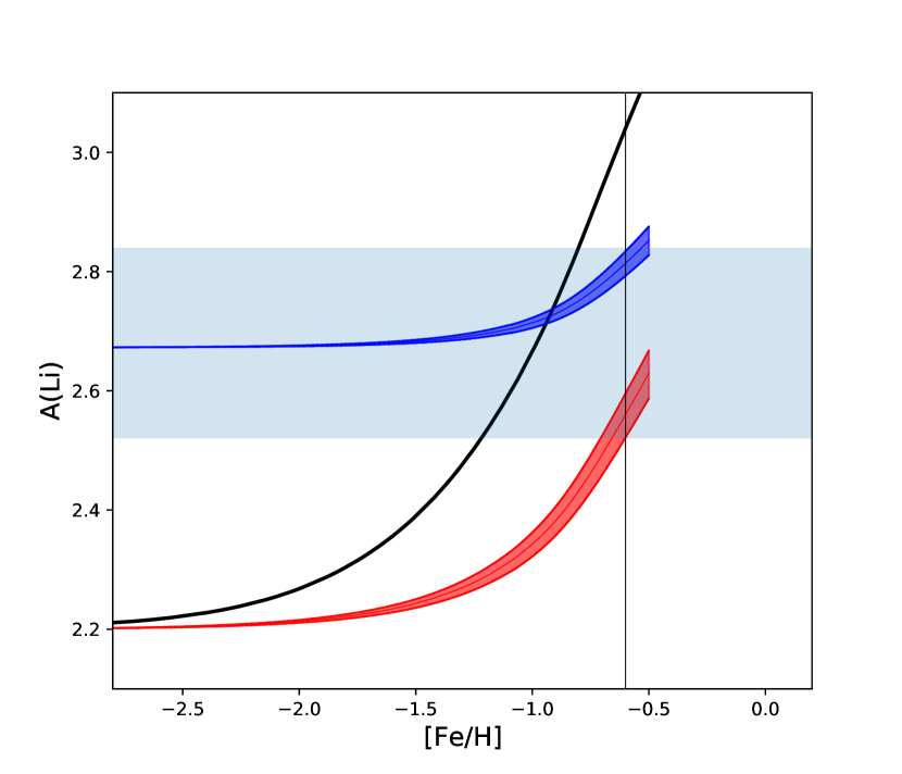
Figure 17: The Li evolution in the SMC assuming the nova yields derived in this paper starting from two different Li initial values: in red the Spite plateau and in blue the CMB+BBN nucleosynthesis. The two curves for each initial lithium abundance and the derived nova yields with their error are shown by shaded regions. The model include astration as well as spallation nucleosynthesis and a modest AGB contribution. The present Li abundance measured in the ISM of SMC derived by Howk et al. (2012) with $\pm 1\sigma$ error is shown with the shaded horizontal band. Finally, the black curve shows the Li evolution derived when a chemical evolution of the SMC but with a Li-yield typical of our Galaxy, namely a factor 4 higher than of the SMC, is considered (Cescutti & Molaro, 2019). Note how much the expected value for $A(Li)$ would be off with respect to the present Li abundance value in the SMC if we consider MW-like yields.

6 Conclusions

After the discovery of ASASSN-19qv in the SMC, we were granted a DDT programme at ESO-VLT with the high-resolution spectrographs UVES and X-shooter, in order to study the spectroscopic evolution of ASASSN-19qv and to search for the ⁷Be isotope in the early epochs of the nova outburst. One year later, and in the middle of the pandemic, we used granted telescope time to observe the outburst of another nova in the SMC, ASASSN20-ni. The target-of-opportunity nature of our program allowed us to observe the nova very soon after its discovery and the first high-resolution spectrum with VLT/UVES was obtained four days later. We summarize the main results here.

• The ⁷Be ii resonance transitions were detected in ASASSN-19qv at two distinct epochs, and also in ASASSN-20ni in all the epochs of the observations.

• We have analysed the outburst spectra in order to infer the amount of ⁷Be, and therefore ⁷Li, synthesised in TNR of both novae. This provided the first estimate of the lithium yield by novae in the SMC, namely N(⁷Li)/N(H) = (5.3 $\pm$ 0.2) $\times$ 10^-6. With a conservative value of $M_{H,ej}=$ 10^-5 M_⊙ we have $M_{{}^{7}Be}=(3.7\pm 0.6)\times 10^{-10}$ M_⊙ per nova event.

• We have also studied two historical novae exploded in the Large Magellanic Cloud which have been followed by the IUE satellite. The IUE LWP spectra of LMC 1991 and LMC 1992 exhibit a strong absorption feature that can be identified as the resonance doublet of singly-ionized ⁷Be ii. The low metallicity of the Large Magellanic Cloud make less likely to explain the feature as a blend of absorption lines of singly ionized metals. By using Mg as a reference element we obtain a ⁷Be ii  abundance of $N(^{7}Be)/N(H)\sim 4.36\times 10^{-6}$, which, despite several uncertainties, is very close to that derived for the novae of the Small Magellanic Cloud. To note that Mg and ⁷Be ii  have similar second ionization potentials and of therefore the ⁷Be ii  yields obtained by using Mg are quite insensitive to the presence of overionization effects in the ejecta.

• When these yields are inserted in a chemical evolution model suited for the SMC they result into a present Li abundance of the order of A(Li)=2.56 when starting form a low primordial ⁷Li value or A(Li)=2.8 when starting from a high primordial value. The observation of present Li in the interstellar gas of the SMC of Howk et al. (2012) of A(Li)=2.68 $\pm$ 0.16 are consistent with both values within 1 $\sigma$ error and precludes from any firm conclusion.

• The evidence of ⁷Be in the CN ejecta observed in the Magellanic Clouds suggests that the thermonuclear reactions giving origin to this isotope during the TNR is effective also in environments characterised by a general sub-solar metallicity, as it is indeed the case for the two main Milky Way satellites. All recent CN explosion simulations have always considered a solar abundance value for the material accreted onto the primary WD in a CN binary system (Casanova et al., 2018; José et al., 2020; Starrfield et al., 2020). Therefore, our result implies the necessity of further simulations, characterised by a sub-Solar metallicity for the matter accreting the primary WD, that can support our finding.

• This result implies that CNe are likely the main lithium factories also in systems external to our Galaxy. Further observations will constrain much better the lithium yield in nearby galaxies, such as the SMC and the LMC. This goal will be easily reachable with the possibility to use advanced high-resolution spectrographs observing the near-UV range such as the proposed CUBES at ESO/VLT (Ernandes et al., 2020).

Data Availability

The data underlying this article will be shared on reasonable request to the corresponding author.

References

- Andrea et al. (1994) Andrea J., Drechsel H., Starrfield S., 1994, A&A, 291, 869
- Astropy Collaboration et al. (2013) Astropy Collaboration et al., 2013, A&A, 558, A33
- Aydi et al. (2018) Aydi E., Buckley D. A. H., Mohamed S., Whitelock P. A., 2018, The Astronomer’s Telegram, 11287, 1
- Aydi et al. (2019) Aydi E., et al., 2019, The Astronomer’s Telegram, 12907, 1
- Aydi et al. (2020) Aydi E., et al., 2020, The Astronomer’s Telegram, 14123, 1
- Bode & Evans (2012) Bode M. F., Evans A., 2012, Classical Novae
- Boggess et al. (1978) Boggess A., et al., 1978, Nature, 275, 372
- Bohlsen (2019a) Bohlsen T. C., 2019a, The Astronomer’s Telegram, 12917, 1
- Bohlsen (2019b) Bohlsen T. C., 2019b, The Astronomer’s Telegram, 12938, 1
- Bonifacio et al. (2015) Bonifacio P., et al., 2015, A&A, 579, A28
- Bouret et al. (2003) Bouret J. C., Lanz T., Hillier D. J., Heap S. R., Hubeny I., Lennon D. J., Smith L. J., Evans C. J., 2003, ApJ, 595, 1182
- Brüns et al. (2005) Brüns C., et al., 2005, A&A, 432, 45
- Bucciarelli et al. (2008) Bucciarelli B., et al., 2008, in Jin W. J., Platais I., Perryman M. A. C., eds, IAU Symposium Vol. 248, A Giant Step: from Milli- to Micro-arcsecond Astrometry. pp 316–319, doi:10.1017/S1743921308019443
- Cameron (1955) Cameron A. G. W., 1955, ApJ, 121, 144
- Cameron & Fowler (1971) Cameron A. G. W., Fowler W. A., 1971, ApJ, 164, 111
- Carrera et al. (2008) Carrera R., Gallart C., Aparicio A., Costa E., Méndez R. A., Noël N. E. D., 2008, AJ, 136, 1039
- Casanova et al. (2018) Casanova J., José J., Shore S. N., 2018, A&A, 619, A121
- Cassatella et al. (2002) Cassatella A., Altamore A., González-Riestra R., 2002, A&A, 384, 1023
- Cescutti & Molaro (2019) Cescutti G., Molaro P., 2019, MNRAS, 482, 4372
- Cescutti et al. (2020) Cescutti G., Molaro P., Fu X., 2020, Mem. Soc. Astron. Italiana, 91, 153
- Choudhury et al. (2018) Choudhury S., Subramaniam A., Cole A. A., Sohn Y. J., 2018, MNRAS, 475, 4279
- Christian et al. (2018) Christian G., et al., 2018, Phys. Rev. C, 97, 025802
- Chugai & Kudryashov (2020) Chugai N. N., Kudryashov A. D., 2020, arXiv e-prints, p. arXiv:2007.07044
- Cioni et al. (2011) Cioni M. R., et al., 2011, The Messenger, 144, 25
- Coc et al. (2014) Coc A., Uzan J.-P., Vangioni E., 2014, J. Cosmology Astropart. Phys., 10, 50
- Cyburt et al. (2016) Cyburt R. H., Fields B. D., Olive K. A., Yeh T.-H., 2016, Reviews of Modern Physics, 88, 015004
- D’Antona & Matteucci (1991) D’Antona F., Matteucci F., 1991, A&A, 248, 62
- Della Valle & Izzo (2020) Della Valle M., Izzo L., 2020, arXiv e-prints, p. arXiv:2004.06540
- Dolphin et al. (2001) Dolphin A. E., Walker A. R., Hodge P. W., Mateo M., Olszewski E. W., Schommer R. A., Suntzeff N. B., 2001, ApJ, 562, 303
- Ernandes et al. (2020) Ernandes H., et al., 2020, in Society of Photo-Optical Instrumentation Engineers (SPIE) Conference Series. p. 1144760 (arXiv:2102.02205), doi:10.1117/12.2562497
- Ferland et al. (2017) Ferland G. J., et al., 2017, Rev. Mex. Astron. Astrofis., 53, 385
- Fields (2011) Fields B. D., 2011, Annual Review of Nuclear and Particle Science, 61, 47
- Fields et al. (2014) Fields B. D., Molaro P., Sarkar S., 2014, preprint, (arXiv:1412.1408)
- Fu et al. (2015) Fu X., Bressan A., Molaro P., Marigo P., 2015, MNRAS, 452, 3256
- Fu et al. (2018) Fu X., et al., 2018, A&A, 610, A38
- Gallagher & Starrfield (1978) Gallagher J. S., Starrfield S., 1978, ARA&A, 16, 171
- Gehrz et al. (1998) Gehrz R. D., Truran J. W., Williams R. E., Starrfield S., 1998, PASP, 110, 3
- Glatt et al. (2008) Glatt K., et al., 2008, AJ, 135, 1106
- Grisoni et al. (2019) Grisoni V., Matteucci F., Romano D., Fu X., 2019, MNRAS, 489, 3539
- Howk et al. (2012) Howk J. C., Lehner N., Fields B. D., Mathews G. J., 2012, Nature, 489, 121
- Hunter (2007) Hunter J. D., 2007, Computing In Science & Engineering, 9, 90
- Izzo et al. (2015) Izzo L., et al., 2015, ApJ, 808, L14
- Izzo et al. (2018) Izzo L., et al., 2018, MNRAS, 478, 1601
- José et al. (2020) José J., Shore S. N., Casanova J., 2020, A&A, 634, A5
- Kafka (2021) Kafka S., 2021, https://www.aavso.org
- Kastner & Bhatia (1995) Kastner S. O., Bhatia A. K., 1995, ApJ, 439, 346
- Korn et al. (2000) Korn A. J., Becker S. R., Gummersbach C. A., Wolf B., 2000, A&A, 353, 655
- Lambert & Reddy (2004) Lambert D. L., Reddy B. E., 2004, MNRAS, 349, 757
- Lanfranchi et al. (2006) Lanfranchi G. A., Matteucci F., Cescutti G., 2006, MNRAS, 365, 477
- Lawler et al. (2017) Lawler J. E., Sneden C., Nave G., Den Hartog E. A., Emrahoğlu N., Cowan J. J., 2017, ApJS, 228, 10
- Leroy et al. (2007) Leroy A., Bolatto A., Stanimirovic S., Mizuno N., Israel F., Bot C., 2007, ApJ, 658, 1027
- Lodders (2019) Lodders K., 2019, arXiv e-prints, p. arXiv:1912.00844
- Lodders et al. (2009) Lodders K., Palme H., Gail H.-P., 2009, Landolt Börnstein,
- Madden et al. (2013) Madden S. C., et al., 2013, PASP, 125, 600
- Matteucci (2021) Matteucci F., 2021, A&ARv, 29, 5
- Matteucci et al. (2021) Matteucci F., Molero M., Aguado D. S., Romano D., 2021, MNRAS, 505, 200
- McConnachie (2012) McConnachie A. W., 2012, AJ, 144, 4
- Molaro et al. (1997) Molaro P., Bonifacio P., Castelli F., Pasquini L., 1997, A&A, 319, 593
- Molaro et al. (2016) Molaro P., Izzo L., Mason E., Bonifacio P., Della Valle M., 2016, MNRAS, 463, L117
- Molaro et al. (2020a) Molaro P., Izzo L., Bonifacio P., Hernanz M., Selvelli P., della Valle M., 2020a, MNRAS, 492, 4975
- Molaro et al. (2020b) Molaro P., Cescutti G., Fu X., 2020b, MNRAS, 496, 2902
- Molaro et al. (2022) Molaro P., et al., 2022, MNRAS, 509, 3258
- Mróz et al. (2016) Mróz P., et al., 2016, ApJS, 222, 9
- Mucciarelli (2014) Mucciarelli A., 2014, Astronomische Nachrichten, 335, 79
- Mukai & Sokoloski (2019) Mukai K., Sokoloski J. L., 2019, Physics Today, 72, 38
- Nidever et al. (2017) Nidever D. L., et al., 2017, AJ, 154, 199
- Payne-Gaposchkin (1957) Payne-Gaposchkin C. H., 1957, The galactic novae.
- Planck Collaboration et al. (2016) Planck Collaboration et al., 2016, A&A, 594, A13
- Prantzos (2012) Prantzos N., 2012, A&A, 542, A67
- Ramírez et al. (2012) Ramírez I., Fish J. R., Lambert D. L., Allende Prieto C., 2012, ApJ, 756, 46
- Romano et al. (1999) Romano D., Matteucci F., Molaro P., Bonifacio P., 1999, A&A, 352, 117
- Sbordone et al. (2010) Sbordone L., et al., 2010, A&A, 522, A26
- Schwarz et al. (2001) Schwarz G. J., Shore S. N., Starrfield S., Hauschildt P. H., Della Valle M., Baron E., 2001, MNRAS, 320, 103
- Selvelli et al. (2018) Selvelli P., Molaro P., Izzo L., 2018, MNRAS, 481, 2261
- Setoodehnia et al. (2018) Setoodehnia K., Marshall C., Kelley J. H., Liang J., Portillo Chaves F., Longland R., 2018, Phys. Rev. C, 98, 055804
- Shappee et al. (2014) Shappee B. J., et al., 2014, ApJ, 788, 48
- Spite (1990) Spite F., 1990, Mem. Soc. Astron. Italiana, 61, 663
- Spite & Spite (1982) Spite F., Spite M., 1982, A&A, 115, 357
- Spitzer (1998) Spitzer L., 1998, Physical Processes in the Interstellar Medium
- Stanimirović et al. (2004) Stanimirović S., Staveley-Smith L., Jones P. A., 2004, ApJ, 604, 176
- Starrfield et al. (1978) Starrfield S., Truran J. W., Sparks W. M., Arnould M., 1978, ApJ, 222, 600
- Starrfield et al. (2020) Starrfield S., Bose M., Iliadis C., Hix W. R., Woodward C. E., Wagner R. M., 2020, ApJ, 895, 70
- Tajitsu et al. (2015) Tajitsu A., Sadakane K., Naito H., Arai A., Aoki W., 2015, Nature, 518, 381
- Tajitsu et al. (2016) Tajitsu A., Sadakane K., Naito H., Arai A., Kawakita H., Aoki W., 2016, ApJ, 818, 191
- Trundle et al. (2007) Trundle C., Dufton P. L., Hunter I., Evans C. J., Lennon D. J., Smartt S. J., Ryans R. S. I., 2007, A&A, 471, 625
- Van Der Walt et al. (2011) Van Der Walt S., Colbert S. C., Varoquaux G., 2011, preprint, (arXiv:1102.1523)
- Ventura & D’Antona (2010) Ventura P., D’Antona F., 2010, MNRAS, 402, L72
- Warner (1989) Warner B., 1989, in Classical Novae. pp 1–16
- Way et al. (2020) Way Z., et al., 2020, The Astronomer’s Telegram, 14122, 1
- Williams (1994) Williams R. E., 1994, ApJ, 426, 279
- Williams (2012) Williams R., 2012, AJ, 144, 98
- Williams et al. (1991) Williams R. E., Hamuy M., Phillips M. M., Heathcote S. R., Wells L., Navarrete M., 1991, ApJ, 376, 721
- Williams et al. (2008) Williams R., Mason E., Della Valle M., Ederoclite A., 2008, ApJ, 685, 451